code-for-first-row = , code-for-last-row = , code-for-first-col = , code-for-last-col =
The Generalized Kauffman-Harary Conjecture is True
Abstract.
For a reduced alternating diagram of a knot with a prime determinant the Kauffman-Harary conjecture states that every non-trivial Fox -coloring of the knot assigns different colors to its arcs. In this paper, we prove a generalization of the conjecture stated nineteen years ago by Asaeda, Przytycki, and Sikora: for every pair of distinct arcs in the reduced alternating diagram of a prime link with determinant there exists a Fox -coloring that distinguishes them.
Key words and phrases:
Determinants of links, double branched cover, Fox colorings, Kauffman-Harary conjecture, knots and links, pseudo colorings.2020 Mathematics Subject Classification:
Primary: 57K10 Secondary: 57M121. History of the alternation conjecture
In 1998, Louis H. Kauffman and Frank Harary formulated the following conjecture [HK]:
Alternation Conjecture.
Let be a reduced, alternating diagram of a knot having determinant , where is prime. Then every non-trivial -coloring of assigns different colors to different arcs.
This conjecture is now known as the Kauffman-Harary conjecture. It was proved for rational knots [KL, PDDGS], Montesinos knots [APS], some Turk’s head knots [DMMS], and for algebraic knots [DS]. In 2009, Thomas W. Mattman and Pablo Solis proved this conjecture using the notion of pseudo colorings. A generalization of this conjecture, known as the generalized Kauffman-Harary (GKH) conjecture, was formulated by Marta M. Asaeda, Adam S. Sikora, and the fifth author in 2004 [APS]. They proved this conjecture for Montesinos links in the same paper. In this paper, we prove it in full generality.
The paper is structured as follows. In the next section we introduce the GKH conjecture and we prove it in Section 3. In Section 4, we reformulate and prove the conjecture for non-prime alternating links. We illustrate the results with some examples in Section 5. In the last section, we discuss pseudo colorings followed by some open questions.
2. Preliminaries
In this section, we state the original and alternate versions of the GKH conjecture. The difference between the original and generalized versions of the conjecture is that the former is about links with prime determinant, while the generalized version is about links with determinant not necessarily prime. It is important to note that the only link whose determinant is prime is the Hopf link.
Generalized Kauffman-Harary Conjecture.
If is a reduced alternating diagram of a prime link , then different arcs of represent different elements of , where denotes the double branched cover of branched along .
The GKH conjecture was formulated in [APS] using the homology of the double branched cover of branched along . In this paper we use a diagrammatic version of this conjecture by using the universal111Analogous to the fundamental group and the fundamental quandle, this group is often called the fundamental group of Fox colorings. group of Fox colorings for a prime link with diagram .
Definition 2.1.
The group is the abelian group whose generators are indexed by the arcs of , denoted by , and whose relations are given by the crossings of . More precisely,
It is known that (see, for example, [Prz1]).
Definition 2.2.
Let be the group of trivial colorings of . This group is embedded in and the quotient group is called the reduced group of Fox colorings. We denote it by .
Notice that, for a diagram of a link , and for non-split alternating links, this group is finite with non-zero determinant.
The first two statements of the following conjecture are equivalent to the original GKH conjecture, while part offers an extension.
Conjecture 2.3 (Alternate forms of the generalized Kauffman-Harary conjecture).
Let be a reduced alternating diagram of an alternating prime link and let denote the absolute value of its determinant.
-
(a)
Let denote the free abelian group . Consider the map Then is injective on the arcs of , that is, for .
-
(b)
The diagram has Fox -colorings , such that for every pair of distinct arcs , there exists such that .
-
(c)
If with , then there are Fox -colorings that distinguish all the arcs of . Note that, is strictly less than the number of crossings of .
Remark 2.4.
Parts (a) and (b) of Conjecture 2.3 are equivalent to each other, since for a finite group , we have , where , with and . In particular, . Thus, we can work with a group or its dual. To distinguish elements in the group we often analyze its homomorphisms (dual elements) into the given ring. See [Lan], for example.
3. Proof of the generalized Kauffman-Harary conjecture
The proof of the GKH conjecture is organized as follows. First, we define the crossing matrix and coloring matrix of a link diagram . Following [MS] we prove that every column of the coloring matrix represents a non-trivial Fox -coloring. Then using the fact that the coloring matrix of the mirror image of is the transpose of , we prove part (b), and equivalently, part (a) of Conjecture 2.3. Additionally, we show that the columns of the coloring matrix generate the group and use this fact to prove part (c) of Conjecture 2.3.
Definition 3.1.
A Fox -coloring of a diagram is a function , satisfying the property that every arc is colored by an element of in such a way that at each crossing the sum of the colors of the undercrossings is equal to twice the color of the overcrossing modulo . That is, if at a crossing the overcrossing is colored by , and the undercrossings are colored by and , then modulo . See Figure 3.1 for an illustration. The group of Fox -colorings of a diagram is denoted by and the number of Fox -colorings is denoted by . Analogous to Definition 2.2, we divide the group by the group of trivial colorings and denote the quotient group by .
The matrix describing the space of colorings is referred to, by Mattman and Solis, as the crossing matrix for a fixed arbitrary ordering of the crossings [MS]. Here we do not assume that the diagram is alternating.
Definition 3.2.
Fix an ordering of the crossings of a reduced link diagram . Then the set of arcs inherits the order of the set of crossings. In this way, the over-arc has the same index as the crossing. The crossing matrix222The alternative, more descriptive, name could be unreduced fundamental Fox colorings matrix. of , denoted by , is an matrix such that each row corresponds to a crossing that gives the relation (see Figure 3.1). The entries of the matrix are defined as follows333It is possible that two under-arcs at a crossing are not distinct. Then the relation becomes . For instance, this may occur for the Hopf link.:
![[Uncaptioned image]](/html/2301.02645/assets/FoxrelationOverpic.png)
| \begin{overpic}[scale={.44}]{Crossingchange.png} \put(80.0,125.0){$c_{k}$} \put(80.0,83.0){$c_{i}$} \put(80.0,40.0){$c_{j}$} \put(92.0,70.0){$a_{i}$} \put(65.0,135.0){$a_{k}$} \put(65.0,50.0){$a_{j}$} \put(385.0,125.0){$c_{k}$} \put(360.0,125.0){$\overline{a_{k}}$} \put(385.0,83.0){$c_{i}$} \put(369.0,95.0){$\overline{a_{i}}$} \put(385.0,40.0){$c_{j}$} \put(360.0,40.0){$\overline{a_{j}}$} \par\end{overpic} |
The following lemma holds only for alternating links and plays an important role in the proof of the GKH conjecture.
Lemma 3.3.
Let be a reduced alternating link diagram with crossing matrix and let be its mirror image. Then the matrix is a crossing matrix for .
Proof.
Denote the crossings of the diagram by and let the over-arc at the crossing be denoted by . Notice that, in the matrix all entries on the diagonal are . We obtain by crossing-change operations and we keep the ordering and names of the crossings. Now, let denote the over-arc at the crossing in the diagram . In the row corresponding to the crossing , suppose the columns corresponding to the arcs and have as entries. Then in the matrix , the column corresponding to must have entries in the rows corresponding to the crossings and ; see Figure 3.2.
∎
Recall that if , then is a finite group whose invariant factor decomposition is , with for all . Notice that, is the minimum number of generators of this group and is the annihilator of the group. Let denote the reduced crossing matrix of , which is the matrix obtained from by removing its last row and last column. We call the arc corresponding to the last column of the base arc. This matrix describes the group . The matrix is a matrix with rational entries. However, is an integral matrix, which we denote by Observe that the columns of modulo represent Fox -colorings of the diagram after coloring the base arc by color .
The following result also holds for reduced non-alternating links.
Theorem 3.4.
Let be a reduced diagram of a link with non-zero determinant. Then the columns of modulo generate the space of Fox -colorings of .
Proof.
Let be the reduced crossing matrix of and let , with for all . After row and column operations, can be reduced to its Smith normal form, denoted by , given below.
Its inverse matrix, , with entries in has the following form.
Thus, we obtain the following integral matrix .
Now, the column of modulo with generates the subgroup of . Since , therefore, the columns of generate the group , as desired.
∎
For alternating diagrams we can prove the following stronger result, which proves part (b), and equivalently, part (a) of Conjecture 2.3.
Theorem 3.5.
Let be a reduced alternating diagram of a prime link. For any two arcs and , there exists a column of which distinguishes them.
Proof.
Suppose the arcs (indexing rows) of the coloring matrix are given by , , …, as shown below.
Recall that, the reduced crossing matrix is obtained from by removing its last row and last column. Now, each column of colors the the remaining first arcs of the diagram. For a complete Fox -coloring of we color the last (base) arc by color . If any for , then column modulo cannot distinguish between the arcs and . If all the entries of the rows corresponding to and are not identical modulo , then they can be automatically distinguished by the column in which they are different.
Step 1: If there is no column of such that mod , then every entry in the row is mod . It follows that in the transpose matrix , the column is the zero column modulo . This would result in the existence of a pseudo coloring of (see Definition 6.1 and [MS]), which is a contradiction. Thus, the base arc can be distinguished from any other arc by some column in modulo .
Step 2: Furthermore, if there are two arcs and with the same color in every column of , then we choose arc as the base arc, which implies that the colors of are equal to zero. So we are back to Step 1.
∎
Theorem 3.6.
If , with , then there are Fox -colorings (not necessarily corresponding to the columns of the coloring matrix) which distinguish all arcs. That is, for every pair of arcs of , one of these -colorings distinguishes them.
Proof.
Denote the generators of the group by , , …, . Every generator is a linear combination of some columns of the coloring matrix modulo (see Theorem 3.4). Therefore, they correspond to some coloring of the diagram . Hence, for every pair of arcs there is a column of modulo that distinguishes them.
∎
Corollary 3.7.
If is the cyclic group ,
-
(a)
then there exists a non-trivial Fox -coloring that distinguishes all arcs.
-
(b)
Additionally, if is a prime number, then the original Kauffman-Harary conjecture holds. That is, every non-trivial Fox -coloring distinguishes all arcs.
Proof.
Part (a) follows directly from Theorem 3.6, for . Part (b) follows because every non-zero element of is its generator.
∎
4. Non-prime alternating links
Theorems 3.5 and 3.6 do not hold as stated for the connected sum of alternating links444The connected sum of alternating links, is an alternating link. For example, see [PBIMW]. (see part (a) of Lemma 4.1). In Theorem 4.2, we present a version of the GKH conjecture which holds for non-prime alternating links.
Lemma 4.1.
[Prz1]
Let be the connected sum of two link diagrams. Then,
-
(a)
the arcs connecting the two components represent the same element in , and
-
(b)
.
Theorem 4.2.
Let , where is a reduced alternating diagram of a prime link , for . Then,
-
(a)
for any pair of arcs different from arcs joining with , there exists a Fox -coloring which distinguishes them, and
-
(b)
there are () Fox -colorings such that any pair of arcs different from the ones joining with , is distinguished by one of them.
Remark 4.3.
Example 4.4.
Let be an alternating diagram of the square knot, that is , with reduced crossing matrix (see Figure 4.1). Then . Observe that columns 3 and 5 of modulo (Figure 4.2) distinguish all pairs of arcs except the ones connecting with Also, the third row (corresponding to the third crossing in the chosen ordering and, therefore, to the third arc) has all zero entries. That is, the third arc cannot be distinguished from the base arc.
| \begin{overpic}[scale={1.7}]{squareknot} \par\put(55.0,60.0){$(1,0)$} \put(29.0,52.0){$(2,0)$} \put(37.0,135.0){$(0,0)$} \put(133.0,65.0){$(0,1)$} \put(105.0,54.0){$(0,2)$} \put(30.0,5.0){$(0,0)$} \par\end{overpic} |
5. Examples of Fox colorings
In this section we study examples of alternating link diagrams and their Fox colorings. For the structure of the group for knots up to 10 crossings, see Appendix C in [BZ].
Example 5.1.
Kauffman and Harary showed that the knot is a counterexample to their conjecture for a knot with non-prime determinant [HK]. We have, and .555It was noticed in [KL] that the Kauffman-Harary conjecture holds for any rational (2-bridge) knot without restrictions on the determinant of the knot. However, as they note, the formulation of the conjecture needs to be changed from “every non-trivial Fox -coloring” to “there exists a Fox -coloring.” See Corollary 3.7. See Figure 5.2 for a Fox -coloring distinguishing all arcs.
| \begin{overpic}[scale={0.8}]{7_7.png} \par\put(170.0,130.0){$1$} \put(142.0,100.0){$2$} \put(53.0,138.0){$4$} \put(75.0,100.0){$7$} \put(2.0,20.0){$12$} \put(70.0,40.0){$20$} \put(195.0,45.0){$0$} \par\end{overpic} |
Example 5.2.
Consider the family of links obtained by closing the braids . These links are sometimes called Turk’s head links and can also be obtained by drawing the Tait diagrams of the wheel graphs . The closed formula for the determinant of the is given in [Prz2]. Examples for and are drawn in Figure 5.3 and their reduced groups of Fox colorings are as follows:
-
(a)
For , is in Rolfsen’s table [Rol]. .
- (b)
Example 5.3.
6. Odds and ends
6.1. Pseudo colorings
An important tool in our proof of Theorem 3.5 is the idea of pseudo colorings. In [MS] and in this paper, it is shown that no pseudo colorings exist for reduced, prime, alternating link diagrams. However, the existence of pseudo colorings can be used to see how far a diagram is from being an alternating link diagram. In this section, we briefly explore this concept. In [MS], Proposition 3.2 depends on the fact that for reduced alternating diagrams the rows of the crossing matrix add to zero. This does not hold for non-alternating diagrams, as we illustrate in the following examples.
Definition 6.1.
Let be a link diagram and . Following Mattman and Solis [MS], we define an -pseudo coloring of as colorings of the arcs of such that, at all but two crossings the Fox coloring convention is satisfied. We denote the other two crossings by and where the coloring conventions are and respectively. To obtain the pseudo colorings as defined in [MS], put .
For an alternating link diagram , our convention was to order crossings first and then, the set of arcs inherits the order of the set of crossings. Compare Definition 3.1. The reason for such a choice is that is the same as . This does not work for non-alternating link diagrams.
In general, we can arbitrarily order crossings and arcs. In Figure 6.1 we give an example of ordering crossings and arcs for the knot . We first choose a base point and an orientation (shown by an arrow on the left-hand side of Figure 6.1). Starting at this base point, we move along the knot and order crossings. Next, arcs can be ordered arbitrarily with the base arc always being the last one. In Figure 6.1 the first coordinate gives the number of the crossing and the second one gives the number of the arc.
| \begin{overpic}[scale={1.7}]{8_19aspretzel} \put(103.0,72.0){$1,5$} \put(103.0,45.0){$2,1$} \put(25.0,30.0){$3,7$} \put(25.0,58.0){$4,4$} \put(25.0,85.0){$5,6$} \put(62.0,85.0){$6,3$} \put(65.0,58.0){$7,8$} \put(65.0,31.0){$8,2$} \par\end{overpic} |
| \begin{overpic}[scale={1.7}]{8_19aspretzel} \par\put(70.0,105.0){$0$} \put(70.0,13.0){$-1$} \put(27.0,27.0){$0$} \put(-3.0,40.0){$0$} \put(-3.0,75.0){$0$} \put(65.0,124.0){$0$} \put(69.0,70.0){$0$} \put(110.0,31.0){$0$} \put(47.0,20.0){$c_{+1}$} \put(103.0,45.0){$c_{+1}$} \par\end{overpic} |
In the following example, we analyze non-split, non-prime alternating diagrams.
Example 6.2.
Let be a non-split, non-prime alternating link diagram. always has a -pseudo coloring using color on and color on . We illustrate this idea for the square knot in Figure 6.2.
| \begin{overpic}[scale={1.7}]{squareknot} \par\put(57.0,70.0){$1$} \put(32.0,78.0){$1$} \put(40.0,132.0){$0$} \put(5.0,103.0){$c_{+1}$} \put(108.0,48.0){$0$} \put(134.0,60.0){$0$} \put(32.0,4.0){$1$} \put(85.0,23.0){$c_{-1}$} \par\end{overpic} |
On the other hand, non-alternating link diagrams often have -pseudo colorings and -pseudo colorings. See Examples 6.3 and 6.4. If the determinant of a knot with diagram is equal to , we have and every column of colors the first arcs of the diagram. Then for a complete -pseudo coloring of , we color the last (base) arc by color .
Example 6.3.
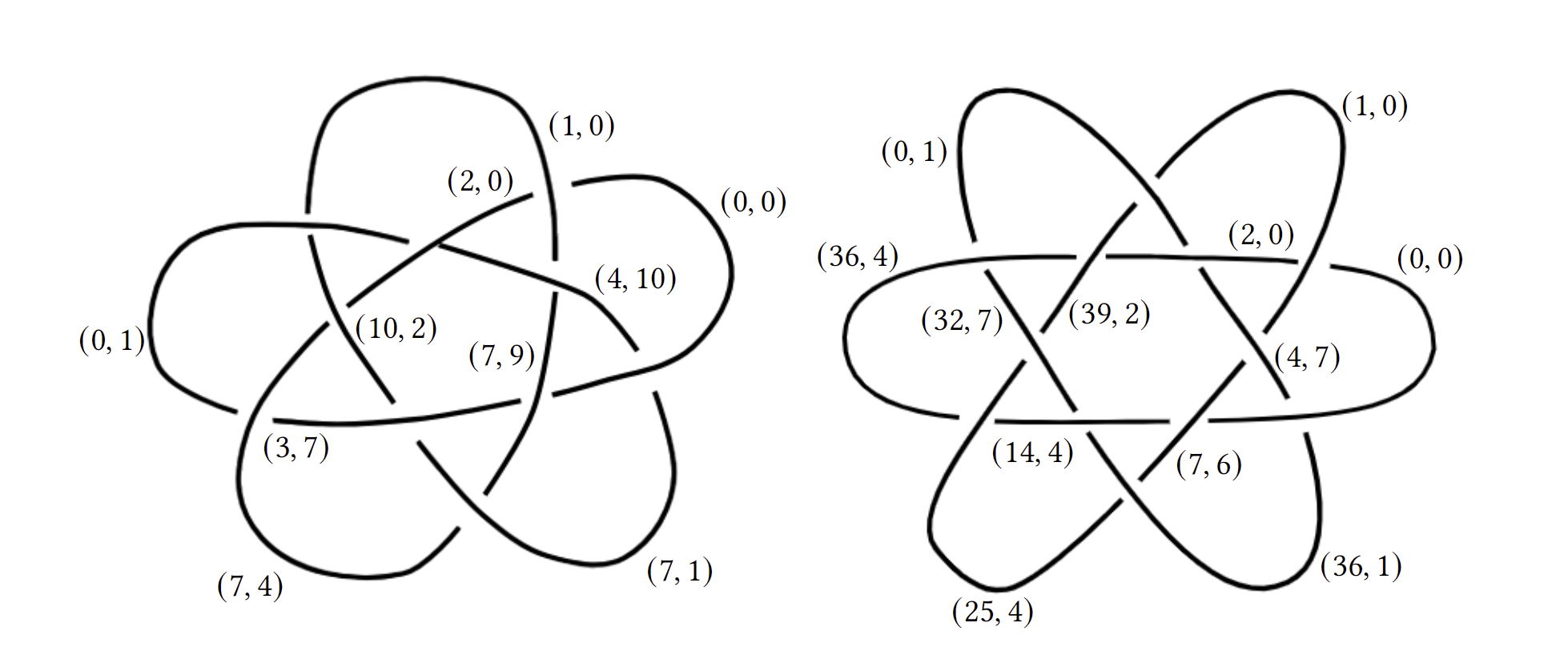
Consider the braid word whose closure is the Conway knot. The determinant of this knot is and its crossing matrix is given in Figure 6.4. The -pseudo coloring given by column and the -pseudo coloring given by column in the matrix shown in Figure 6.5 are illustrated in Figure 6.3 on the left and on the right, respectively.
| \begin{overpic}[scale={0.9}]{CK} \par\put(55.0,150.0){$2$} \put(35.5,118.0){$-8$} \put(40.0,108.0){$-5$} \put(42.0,86.0){$-2$} \put(5.0,222.0){$5$} \put(1.0,110.0){$0$} \put(20.0,210.0){$9$} \put(18.0,165.0){$6$} \put(18.0,149.0){$3$} \put(60.0,100.0){$-3$} \put(3.0,72.0){$1$} \put(50.0,60.0){$c_{+1}$} \put(14.0,76.0){$c_{+1}$} \par\end{overpic} |
| \begin{overpic}[scale={0.9}]{CK} \par\put(55.0,150.0){$6$} \put(35.5,118.0){$-33$} \put(38.5,108.0){$-21$} \put(42.0,86.0){$-9$} \put(5.0,225.0){$21$} \put(1.0,110.0){$0$} \put(20.0,212.0){$39$} \put(13.0,165.0){$26$} \put(13.0,149.0){$13$} \put(60.0,100.0){$-13$} \put(3.0,72.0){$3$} \put(50.0,60.0){$c_{-1}$} \put(55.0,130.0){$c_{+1}$} \par\end{overpic} |
Example 6.4.
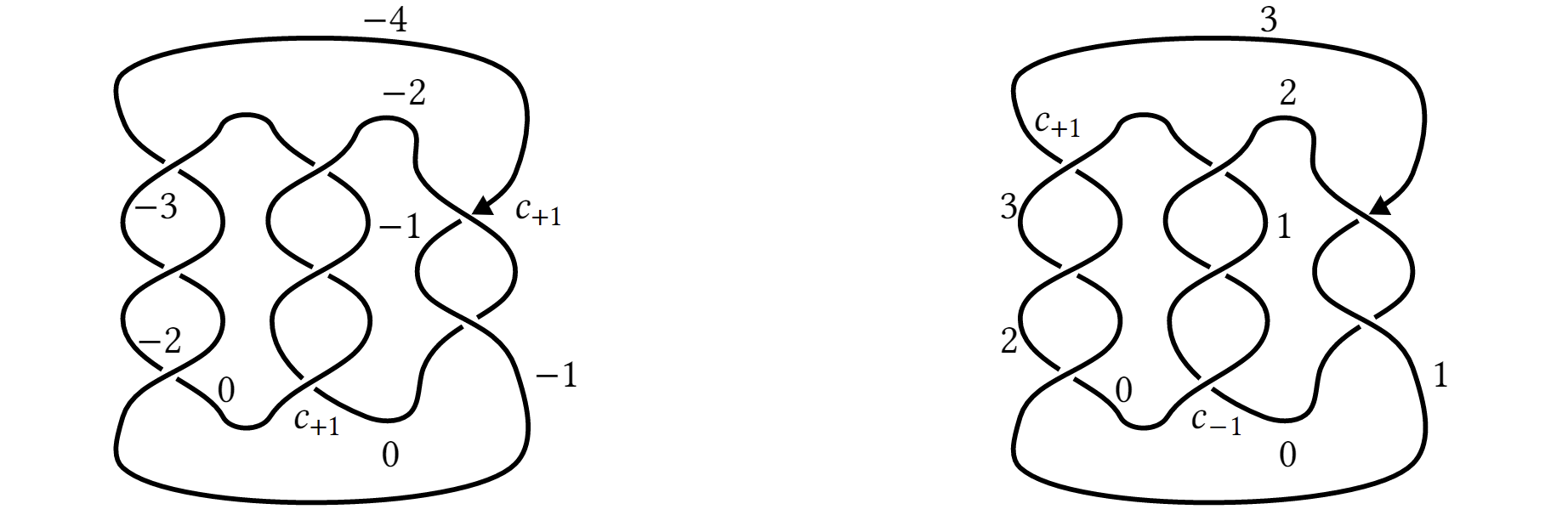
Consider the torus knot with diagram and crossings and arcs ordered as illustrated in Figure 6.1 . Its crossing matrix is shown in Figure 6.7. Three columns of (shown in Figure 6.8) are integral and they yield -pseudo colorings. Column 5 gives a -pseudo coloring (shown on the right in Figure 6.6) and columns 1 and 2 give -1-pseudo colorings. The -pseudo coloring corresponding to column is shown on the left of Figure 6.6.
Non-alternating link diagrams always have -pseudo colorings, as we describe in the following remark.
Remark 6.5.
Let be a non-alternating link diagram.
-
(1)
Every integral column of leads to some -pseudo coloring.
-
(2)
has an -pseudo coloring. This follows from the fact that every non-alternating diagram has a tunnel of length at least two. Now, we can color by coloring one of the arcs of the tunnel by color and all other arcs by color to get the -pseudo coloring. An example of such a coloring is shown on the right-hand side of Figure 6.1.
6.2. Future directions
The Kauffman-Harary conjecture was extended to the case of virtual knots by Mathew Williamson [Wil] and proved by Zhiyun Cheng [Che]. A natural question is to ask whether the conjecture in [APS] holds for virtual links whose determinants are not prime. Another path of further research is to look for a natural generalization to non-alternating diagrams using a set theoretic Yang-Baxter operator or a general Yang-Baxter operator.
An interesting prospect is to approach the generalized Kauffman-Harary conjecture from the perspective of incompressible surfaces in the double branched cover of branched along . This was outlined in [APS] with the hope of proving the GKH conjecture. Now that the GKH conjecture is proved, we can proceed in the opposite direction and analyze incompressible surfaces in .
Acknowledgements
The first author acknowledges the support of Dr. Max Rössler, the Walter Haefner Foundation, and the ETH Zürich Foundation. The third author acknowledges the support of the National Science Foundation through Grant DMS-2212736. The fourth author was supported by the American Mathematical Society and the Simons Foundation through the AMS-Simons Travel Grant. The fifth author was partially supported by the Simons Collaboration Grant 637794.
References
- [APS] M. M. Asaeda, J. H. Przytycki, A. S. Sikora, Kauffman-Harary conjecture holds for Montesinos knots. J. Knot Theory Ramifications 13 (2004), no. 4, 467–477. arXiv:math/0305415 [math.GT].
- [BZ] G. Burde, H. Zieschang, Knots. Second edition. De Gruyter Studies in Mathematics, 5. Walter de Gruyter & Co., Berlin, 2003. xii+559 pp. ISBN: 3-11-017005-1.
- [Che] Z. Cheng, Kauffman-Harary conjecture for alternating virtual knots. J. Knot Theory Ramifications 24 (2015), no. 8, 1550046, 13 pp. arXiv:1310.4271 [math.GT].
- [DS] D. B. Damiano, E. M. Sennott, Coloring algebraic knots and links. J. Knot Theory Ramifications 17 (2008), no. 5, 553–578.
- [DMMS] N. E. Dowdall, T. W. Mattman, K. Meek, P. R. Solis, On the Harary-Kauffman conjecture and Turk’s head knots. Kobe J. Math. 27 (2010), no. 1-2, 1–20. arXiv:0811.0044 [math.GT].
- [HK] F. Harary, L. H. Kauffman, Knots and graphs. I. Arc graphs and colorings. Adv. in Appl. Math. 22 (1999), no. 3, 312-337.
- [Hos] J. Hoste, The enumeration and classification of knots and links. Handbook of knot theory, 209–232, Elsevier B. V., Amsterdam, 2005.
- [KL] L. H. Kauffman, S. Lambropoulou, On the classification of rational tangles. Adv. in Appl. Math. 33 (2004), no. 2, 199–237.arXiv:math/0311499 [math.GT].
- [Lan] S. Lang, Algebra. Revised third edition. Graduate Texts in Mathematics, 211. Springer-Verlag, New York, 2002. xvi+914 pp. ISBN: 0-387-95385-X.
- [Men] W. Menasco, Closed incompressible surfaces in alternating knot and link complements. Topology 23 (1984), no. 1, 37–44.
- [MS] T. W. Mattman, P. Solis, A proof of the Kauffman-Harary conjecture. Algebr. Geom. Topol. 9 (2009), no. 4, 2027–2039. arXiv:0906.1612 [math.GT].
- [PDDGS] L. Person, M. Dunne, J. DeNinno, B. Guntel, L. Smith. Colorings of rational, alternating knots and links, Preprint (2002).
- [Prz1] J. H. Przytycki, 3-coloring and other elementary invariants of knots. Knot theory (Warsaw, 1995), 275–295, Banach Center Publ., 42, Polish Acad. Sci. Inst. Math., Warsaw, 1998. arXiv:math/0608172 [math.GT].
- [Prz2] J. H. Przytycki, From Goeritz matrices to quasi-alternating links. The mathematics of knots, 257–316, Contrib. Math. Comput. Sci., 1, Springer, Heidelberg, 2011. arXiv:0909.1118 [math.GT].
- [PBIMW] J. H. Przytycki, R. P. Bakshi, D. Ibarra, G. Montoya-Vega, D. Weeks, Lectures in Knot Theory: An Exploration of Contemporary Topics, Springer Universitext, recommended for publication, December 2022.
- [Rol] D. Rolfsen, Knots and links. Mathematics Lecture Series, No. 7. Publish or Perish, Inc., Berkeley, Calif., 1976. ix+439 pp. (third edition, AMS Chelsea Publishing, 2003).
- [Thi] M. B. Thistlethwaite, Knot tabulations and related topics, Aspects of topology, LMS Lecture Notes Series, 93, 1985, 176.
- [Wil] M. Williamson, Kauffman-Harary Conjecture for Virtual Knots (2007). USF Tampa Graduate Theses and Dissertations. https://digitalcommons.usf.edu/etd/3916.