Trajectories for the Optimal Collection of Information

Abstract

We study a scenario where an aircraft has multiple heterogeneous sensors collecting measurements to track a target vehicle of unknown location. The measurements are sampled along the flight path and our goals to optimize sensor placement to minimize estimation error. We select as a metric the Fisher Information Matrix (FIM), as “minimizing” the inverse of the FIM is required to achieve small estimation error. We propose to generate the optimal path from the Hamilton–Jacobi (HJ) partial differential equation (PDE) as it is the necessary and sufficient condition for optimality. A traditional method of lines (MOL) approach, based on a spatial grid, lends itself well to the highly non-linear and non-convex structure of the problem induced by the FIM matrix. However, the sensor placement problem results in a state space dimension that renders a naive MOL approach intractable. We present a new hybrid approach, whereby we decompose the state space into two parts: a smaller subspace that still uses a grid and takes advantage of the robustness to non-linearities and non-convexities, and the remaining state space that can be found efficiently from a system of ODEs, avoiding formation of a spatial grid.

1 Introduction

We present a method to optimize vehicle trajectories to gain maximal information for target tracking problems. The scenario currently being studied is an aircraft receiving passive information from sensors rigidly mounted to the airframe. These sensors include, but are not limited to, infrared or visible spectrum, as well as RF receivers that measure the frequency shifts from an external transmitter. The measurements are sampled in order to determine the location of a target vehicle. The placement of the sensors is determined by the path of the aircraft, influencing how much information is gained as well as the overall effectiveness of estimating where the target is located. By optimizing the trajectory, we can achieve maximum information gain, and hence the greatest accuracy in localizing the target.

This problem is a generalization of what appeared in [1], where the path of the vehicle was fixed and a subset of measurements were selected only from along this path. In this context we optimize a metric of the cumulative Fisher Information Matrix (FIM) of the aircraft path, which is motivated by its connection to the (Bayesian) Cramér-Rao lower bound [2]. The logdet metric is chosen as this gives a D-optimal estimate, essentially corresponding to minimizing the volume of the error ellipsoid, and additionally provides favorable numeric properties. It is worth noting that while the focus of this paper is the logdet metric, other metrics may be considered, provided the metric meets certain conditions that are outlined in what follows in the paper. Of particular interest would be the trace of the inverse metric, as that gives the A-optimal estimate, effectively minimizing the mean-square estimate error. Analysis of the trace of the inverse metric is outside the scope of this paper and will be investigated in future work.

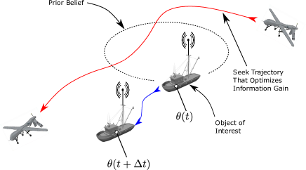
Figure 1: An illustration of the target tracking problem. An aircraft collects measurement for sensors as it flies along a path, attempting to estimate the location of the ship, denoted here as $\theta$. Modifying the path of the vehicle can greatly improve the estimation performance.

We formulate the problem in such a way that the optimal value function satisfies a Hamilton-Jacobi (HJ) partial differential equation (PDE), from which the optimal trajectories immediately follow. Naively, a solution of the corresponding HJ PDE using a grid-based method would have many advantages since they handle the non-linear and non-convex problems that arises in FIM-based optimization. However, the sensor estimation problem induces a state space dimension that renders typical grid-based methods [3] for PDE solutions intractable due to the exponential dimensional scaling of such methods. Recognition of this problem is not new, and the phrase “curse of dimensionality” was coined decades ago by Richard Bellman [4]. This creates a large gap between the rigorous theory of HJ equations and practical implementation on many problems of interest, especially vehicle planning and coordination problems.

New research has emerged in an attempt to bridge this technological gap, including trajectory optimization approaches [5, 6, 7], machine learning techniques [8, 9, 10], and sub-problem decomposition [11, 12]. The structure of the sensor placement problem lends itself well to the later strategy. Unique in this context, though, is that we do not need to abandon spatial grids entirely, instead forming a hybrid approach. This leverages the strength of grid-based methods in dealing with the non-convexities that commonly arise when using the FIM matrix, but restricts their applications to a small subspace of the problem.

In what follows we formally introduce the sensor estimation problem and form its corresponding HJ PDE. We then proceed to show a new hybrid method of lines (MOL) approach that involves decomposing the state space. and conclude with simulated results of the optimal trajectories that result from heterogeneous sensors tracking the location of a mobile target. Section 2 shows how the information collecting problem gives rise to nonlinear dynamics with a cascade structure, that the input only directly affects one first subcomponent of the state, whereas the optimization criteria only depends on a second subcomponent. Section 3 addresses the optimal control of this type of systems using the HJ PDE and the classical MOL. Section 4, develops the theory needed for the new hybrid method of lines, which is applicable to systems in a cascade form. This type of systems arises naturally in formation collecting, but the hybrid methods of lines can be applied to the optimal of more general cascade systems. Section 5 specializes the hybrid MOL to the information collection. Section 6 includes simulation results for a particular vehicle model and sensor type.

2 The Vehicle Sensing Problem

We choose as our vehicle a Dubin’s car [13] and denote by $\left(X,Y,\psi\right):=x\in{\mathcal{X}}:={\mathbb{R}}^{2}\times\text{SO}\left(2\right)$ the vehicle state where $X$ and $Y$ are the rectangular positional coordinates of the vehicle center and $\psi$ is the heading angle. The dynamics are defined by

$$\frac{d}{ds}x\left(s\right) =f\left(x\left(s\right)\right)+Bu\left(s\right),\,\,\text{a.e.}\,s\in\left[0,t\right]$$ (1)

where

$$f\left(x\right)=\left[\begin{array}[]{c}v\cos\psi\\ v\sin\psi\\ 0\end{array}\right],\,B=\left[\begin{array}[]{c}0\\ 0\\ 1\end{array}\right],$$ (2)

where $u\left(s\right)\in U:=\left[-\omega_{\max},\omega_{\max}\right]$ is the allowable control set of turn rates and $v$ is the fixed forward speed of the vehicle. The admissible control set is defined as

$$U\left[0,t\right]:=\left\{u\left(\cdot\right):\left[0,t\right]\rightarrow U\,|\,u\left(\cdot\right)\,\text{is measurable}\right\}.$$ (3)

Our method applied to vehicles that can be expressed in the general form $\left(\ref{eq:state dynamics}\right)$, which includes the Dubins vehicle in $\left(\ref{eq:f and B def}\right)$. The Dubins vehicle with bounded turning rate is particularly interesting because it is a low-dimensional model that generates trajectories that are easy to track by an aircraft flying at constant speed and altitude.

The vehicle defined above has a group of rigidly attached sensors collecting measurements. The measurements, denoted as $y$, are sampled in order to determine an unknown random variable, $\theta$. The measurements are assumed to be random variables dependent on $\theta$ with density function

$$y\sim\rho\left(y|\theta\right).$$

Assuming that all measurements $y$ are conditionally independent given $\theta$, the cumulative Bayesian Fisher Information Matrix (FIM) associated with the estimation of $\theta$ is of the form

$$\text{FIM}\left(t,x,u\left(\cdot\right)\right):=Q_{0}+\int_{0}^{t}Q\left(\gamma\left(s;x,u\left(\cdot\right)\right)\right)ds,$$

where

$$Q\left(x\right):={\mathbb{E}}_{\theta}\left[Q\left(x;\theta\right)\right],$$ (4)

with

$$Q\left(x;\theta\right):={\mathbb{E}}_{y}\left[\left(\frac{\partial\log\rho\left(y|\theta,x\right)}{\partial\theta}\right)^{\top}\left(\frac{\partial\log\rho\left(y|\theta,x\right)}{\partial\theta}\right)\right],$$ (5)

and

$$Q_{0}:={\mathbb{E}}_{\theta}\left[\left(\frac{\partial\log\rho\left(\theta\right)}{\partial\theta}\right)^{\top}\left(\frac{\partial\log\rho\left(\theta\right)}{\partial\theta}\right)\right],$$

where $\rho\left(\theta\right)$ is the a-priori probability density function for $\theta$. The formula above assumes a scenario where the measurement, $y\left(t\right)$, is collected by one sensor or by multiple independent sensors that generate at the same (constant) sampling rate. When multiple independent sensors collect measurements at constant but different sampling rates, the FIM matrix can be factored for each sensor $i$:

$$Q\left(t,x,u\left(\cdot\right)\right)=\sum_{i}F^{i}Q^{i}\left(\gamma\left(s;x,u\left(\cdot\right)\right)\right),$$

where $F^{i}$ is the sampling rate of the $i$-th sensor. The above matrices are given from [14], where the expectation over $y$ in $\left(\ref{eq:Inner Q(x;theta)}\right)$ is given in closed form for some distributions, see for example [1, Sec. 5]. While the outer expectation over $\theta$ in $\left(\ref{eq:Q(x)}\right)$ is rarely known in closed form, many approximation schemes can be employed, for example Monte Carlo sampling or Taylor series expansion.

The placement of the sensors is determined by the path of the aircraft, influencing how much information is gained as well the overall effectiveness of estimating $\theta$. Therefore we optimize the trajectory to achieve maximum information gain, and hence the greatest performance in estimating $\theta$ from the measurements $y$. For a given initial state $x\in{\mathcal{X}}$ and terminal time $t\in\left[0,\infty\right)$, we define the following cost functional:

$$J\left(t,x,u\left(\cdot\right)\right):=G\left(\text{CFIM}\left(t,x,u\left(\cdot\right)\right)\right)+\log\det\left(Q_{0}\right),$$ (6)

where

$$G\left(x,z\right):=-\log\det\left(\text{vec}^{-1}z\right),$$

We denote by $V\left(t,x\right)$ the value function defined as

$$V\left(t,x\right) =\underset{u\left(\cdot\right)\in U\left[0,t\right]}{\text{inf}}\,J\left(t,x,u\left(\cdot\right)\right),$$ (7)

which can be interpreted as the maximal information gain for a family of trajectory optimization problems parameterized by initial state $x\in{\mathcal{X}}$ and terminal time $t\in\left[0,\infty\right)$.

The cost functional in $\left(\ref{eq:original problem}\right)$ is not in a standard form, so we convert the problem into a common standard, the so-called Mayer form. To do this we augment the state vector with $z\in{\mathcal{Z}}:=\text{dom}\left(G\right)$. Our new state becomes

$$\chi:=\left(x,z\right)^{\top},$$

with augmented dynamics

$$\frac{d}{ds}\chi\left(s\right)=\hat{f}\left(\chi\left(s\right),u\left(s\right)\right)=\left[\begin{array}[]{c}f\left(x\left(s\right)\right)\\ \ell\left(x\left(s\right)\right)\end{array}\right]+\left[\begin{array}[]{c}B\\ {\bf 0}\end{array}\right]u\left(s\right),$$ (8)

with

$$\ell\left(x\left(s\right)\right):=\text{vec}\left(Q\left(x\left(s\right)\right)\right),$$

where vec is the vectorize operator that reshapes a matrix into a column vector and ${\bf 0}$ is a vector of zeros of the same number of elements as the augmented variable $z$. If we fix the $z$ initial condition such that

$$z=\text{vec}\left(Q_{0}\right),$$ (9)

then the cost functional $\left(\ref{eq:original metric}\right)$ can equivalently written as

$$J\left(t,x,u\left(\cdot\right)\right)=J\left(t,\chi,u\left(\cdot\right)\right)=G\left(\text{vec}^{-1}\left(z\right)\right),$$ (10)

where we denote by $Z=\text{vec}^{-1}\left(z\right)$ the inverse operator such that

$$\text{vec}\left(\text{vec}^{-1}\left(z\right)\right)=z.$$

Hereafter we will denote by $\tilde{G}$ as the function $G$ with the input reshaped as a function of $z$ with

$$\tilde{G}\left(z\right):=G\left(\text{vec}^{-1}\left(z\right)\right).$$ (11)

Likewise the value function is equivalently written as

$$V\left(t,\chi\right)=\underset{u\left(\cdot\right)\in U\left[0,t\right]}{\text{inf}}\,J\left(t,\chi,u\left(\cdot\right)\right).$$ (12)

3 Decomposition of Coupled Systems

The approach we will develop to solve $\left(\ref{eq:new value function}\right)$ is applicable to a more general class of cascade systems that we introduce in this section, and for which we discuss the use of HJ methods for optimal control. Denote by $\chi:=\left(x,z\right)^{\top}$ where $x\in{\mathcal{X}}={\mathbb{R}}^{n}$ and $z\in{\mathcal{Z}}={\mathbb{R}}^{m}$. The state has coupled dynamics as follows:

$$\begin{cases}\dot{x}\left(s\right)=f\left(x\left(s\right)\right)+g\left(x\left(s\right)\right)u\left(s\right)&\text{a.e}\,s\in\left[0,t\right]\\ \dot{z}\left(s\right)=\ell\left(x\left(s\right)\right),\end{cases}$$ (13)

with $u\in U$, where $U$ is a closed convex set. We denote by $\left[0,t\right]\ni s\mapsto\gamma\left(s;x_{0},u\left(\cdot\right)\right)\in{\mathbb{R}}^{n}$ the $x$ state trajectory that evolves in time according to $\left(\ref{eq:state dynamics}\right)$ starting from initial state $x_{0}$ at $t=0$. The trajectory $\gamma$ is a solution of $\left(\ref{eq:state dynamics}\right)$ in that it satisfies $\left(\ref{eq:state dynamics}\right)$ almost everywhere:

$$\begin{cases}\dot{\gamma}\left(s;x_{0},u\left(\cdot\right)\right)=f\left(\gamma\left(s;x_{0},u\left(\cdot\right)\right)\right)+g\left(\gamma\left(s;x_{0},u\left(\cdot\right)\right)\right)u,\\ \gamma\left(0;x_{0},u\left(\cdot\right)\right)=x_{0}.\end{cases}$$ (14)

Likewise, we denote by $\left[0,t\right]\ni s\mapsto\xi\left(s;\chi_{0},u\left(\cdot\right)\right)$ the trajectory of the $z$ variable and it satisfies the following almost everywhere:

$$\begin{cases}\frac{d}{ds}\xi\left(s;\chi_{0},u\left(\cdot\right)\right)=\ell\left(\gamma\left(s;x_{0},u\left(\cdot\right)\right)\right),\\ \xi\left(0;\chi_{0},u\left(\cdot\right)\right)=z_{0}.\end{cases}$$ (15)

Note that the trajectory can be found directly from the expression:

$$\xi\left(s;\chi_{0},u\left(\cdot\right)\right):=z_{0}+\int_{0}^{s}\ell\left(\gamma\left(\tau;x_{0},u\left(\cdot\right)\right)\right)d\tau.$$ (16)

Denote $G:{\mathbb{R}}^{m}\rightarrow{\mathbb{R}}$ as the terminal cost function such that the mapping

$${\mathcal{Z}}\ni z\mapsto G\left(z\right)\in{\mathbb{R}},$$

We define the cost functional

$$J\left(t,\chi,u\left(\cdot\right)\right):=G\left(\xi\left(t;\chi,u\left(\cdot\right)\right)\right),$$

and the associated value function as

$$V\left(t,\chi\right):=\underset{u\left(\cdot\right)\in U\left[0,t\right]}{\text{inf}}J\left(t,\chi,u\left(\cdot\right)\right),$$

where $U\left[0,t\right]$ is defined as in $\left(\ref{eq:allowable control sequence}\right)$.

We denote by

$$\hat{f}\left(\chi,u\right):=\left[\begin{array}[]{c}f\left(x\right)+g\left(x\right)u\\ \ell\left(x\right)\end{array}\right],$$

the joint vector field in $\left(\ref{eq: Coupled Gen. System}\right)$. We assume that $\hat{f}$ , $U$, and $G$ satisfy the following regularity assumptions:

(F1)

$\left(U,d\right)$ is a separable metric space.

(F2)

The maps $\hat{f}:{\mathcal{X}}\times U\rightarrow{\mathbb{R}}^{n+m}$ and $G:{\mathcal{Z}}\rightarrow{\mathbb{R}}$ are measurable, and there exists a constant $L>0$ and a modulus of continuity $\omega:\left[0,\infty\right)\rightarrow\left[0,\infty\right)$ such that for $\varphi\left(\chi,u\right)=\hat{f}\left(\chi,u\right),G\left(z\right)$, we have for all $\chi,\chi^{\prime}\in{\mathcal{X}}\times{\mathcal{Z}}$, and $u,u^{\prime}\in U$

$$\left|\varphi\left(\chi,u\right)-\varphi\left(\chi^{\prime},u^{\prime}\right)\right|\leq L\left\|\chi-\chi^{\prime}\right\|+\omega\left(d\left(u,u^{\prime}\right)\right),$$

and

$$\left|\varphi\left({\bf 0},u\right)\right|\leq L.$$

(F3)

The maps $\hat{f}$, and $G$ are $C^{1}$ in $\chi$, and there exists a modulus of continuity $\omega:\left[0,\infty\right)\rightarrow\left[0,\infty\right)$ such that for $\varphi\left(\chi,u\right)=\hat{f}\left(\chi,u\right),G\left(z\right)$, we have for all $\chi,\chi^{\prime}\in\mathcal{X}\times\mathcal{Z}$, and $u,u^{\prime}\in U$

$$\left|\varphi_{\chi}\left(\chi,u\right)-\varphi_{\chi}\left(\chi^{\prime},u^{\prime}\right)\right|\leq\omega\left(\left\|\chi-\chi^{\prime}\right\|+d\left(u,u^{\prime}\right)\right).$$

3.1 Hamilton–Jacobi Formulation

Under a set of mild Lipschitz continuity assumptions, there exists a unique value function $\left(\ref{eq:new value function}\right)$ that satisfies the following Hamilton–Jacobi (HJ) equation [15] with $V\left(t,\chi\right)$ being the viscosity solution of the partial differential equation (PDE) for $s\in\left[0,t\right]$

$$V_{s}\left(s,\chi\right)+{\mathcal{H}}\left(\chi,V_{\chi}\left(s,\chi\right)\right) =0,$$ (17)

$$V\left(0,\chi\right) =G\left(z\right),$$

where $\sigma:=\left(p,\lambda\right)^{\top}$ and

$${\mathcal{H}}\left(\chi,\sigma\right):=\underset{u\in U}{\min}H\left(\chi,u,\sigma\right),$$ (18)

with the Hamiltonian, $H$, defined by

$$H\left(\chi,u,\sigma\right) =\left\langle\left[\begin{array}[]{c}f\left(x\right)+g\left(x\right)u\\ \ell\left(x\right)\end{array}\right],\left[\begin{array}[]{c}p\\ \lambda\end{array}\right]\right\rangle$$

$$=\left\langle f\left(x\right),p\right\rangle+\left\langle g\left(x\right)u,p\right\rangle+\left\langle\ell\left(x\right),\lambda\right\rangle.$$

In the case where the set $U$ is bounded by a norm, i.e.

$$U=\left\{u\in{\mathbb{R}}^{n_{u}}|\left\|u\right\|\leq c\right\},$$ (19)

for some $c$, then $\left(\ref{eq:Optimal Hamiltonian-1}\right)$ is given in closed form by

$${\mathcal{H}}\left(\chi,\rho\right)=\left\langle f\left(x\right),p\right\rangle+\left\|g\left(x\right)^{\top}p\right\|_{*}+\left\langle\ell\left(x\right),\lambda\right\rangle,$$ (20)

where $\left\|\left(\cdot\right)\right\|_{*}$ is the dual norm to $\left\|\left(\cdot\right)\right\|$ in $\left(\ref{eq:general control set}\right)$. We denote by $\pi$ the control that optimizes the Hamiltonian and is given by

$$\pi\left(s,\chi\right):=\underset{u\in U}{\arg\,\min}H\left(\chi,u,V_{\chi}\left(s,\chi\right)\right).$$

We note here that under mild assumptions, the viscosity solution of $\left(\ref{eq:HJB Equation-1}\right)$ is Lipschitz continuous in both $s$ and $\chi$ [16, Theorem 2.5, p. 165]. This implies by Rademacher’s theorem [17, Theorem 3.1.6, p. 216] the value function is differentiable almost everywhere. For what follows, we assume that the value function has continuous first and second derivatives. The points where this fails to be true only exists on a set of measure zero, and any practical implementation of the method presented will only evaluate points where the first and second derivatives exist. A characterization of the differentiability of the value function is outside the scope of this paper and a full rigorous treatment will appear in forthcoming work.

3.2 Necessary Conditions of the Optimal Trajectories

Fix $x\in{\mathcal{X}}$ and $z\in{\mathcal{Z}}$ as initial conditions and fix the terminal time $t$. Denote by $\bar{\gamma}\left(s\right)$ and $\bar{\xi}\left(s\right)$ as the optimal state trajectories such that

$$\bar{\gamma}\left(s\right):=\bar{\gamma}\left(s;\chi\right)=\gamma\left(s;x,\bar{u}\left(\cdot;\chi\right)\right),$$

and

$$\bar{\xi}\left(s\right):=\bar{\xi}\left(s;\chi\right)=\xi\left(s;x,z,\bar{u}\left(\cdot;\chi\right)\right),$$

such that $\bar{u}$ optimizes $\left(\ref{eq:new value function}\right)$. By Pontryagin’s theorem [18] there exists adjoint trajectories $p\left(s\right):=p\left(s;\chi\right)$ and $\lambda\left(s\right):=\lambda\left(s;\chi\right)$ such that the function

$$\left[0,t\right]\ni s\mapsto\left(\bar{\gamma}\left(s\right),\bar{\xi}\left(s\right),p\left(s\right),\lambda\left(s\right)\right)$$ (21)

is a solution of the characteristic system

$$\begin{cases}\dot{\bar{\gamma}}\left(s\right)={\mathcal{H}}_{p}\left(\bar{\gamma}\left(s\right),\bar{\xi}\left(s\right),p\left(s\right),\lambda\left(s\right)\right),\\ \dot{\bar{\xi}}\left(s\right)={\mathcal{H}}_{\lambda}\left(\bar{\gamma}\left(s\right),\bar{\xi}\left(s\right),p\left(s\right),\lambda\left(s\right)\right),\\ \dot{p}\left(s\right)=-{\mathcal{H}}_{x}\left(\bar{\gamma}\left(s\right),\bar{\xi}\left(s\right),p\left(s\right),\lambda\left(s\right)\right),\\ \dot{\lambda}\left(s\right)=-{\mathcal{H}}_{z}\left(\bar{\gamma}\left(s\right),\bar{\xi}\left(s\right),p\left(s\right),\lambda\left(s\right)\right),\end{cases}$$ (22)

almost everywhere $s\in\left[0,t\right]$ with boundary conditions

$$p\left(t\right)={\bf 0},\,\,\lambda\left(t\right)=G_{z}\left(\bar{\xi}\left(t\right)\right).$$

3.3 Numerical Approximations Viscosity Solutions to First-Order Hyperbolic PDEs

Traditional methods for computing the viscosity solution to $\left(\ref{eq:HJB Equation-1}\right)$ rely on constructing a discrete grid of points. This is typically chosen as a Cartesian grid, but many other grid types exist. The value function is found using a method of lines (MOL) approach by the solving the following family of ODEs, pointwise at each grid point $\chi^{k}=\left(x^{k},z^{k}\right)\in{\mathcal{S}}:={\mathcal{X}}\times{\mathcal{Z}}$:

$$\begin{cases}\dot{\phi}\left(s,\chi^{k}\right)=-{\mathcal{H}}\left(\chi^{k},D_{\chi}\phi\left(s,\chi^{k}\right)\right),&s\in\left[0,t\right]\\ \phi\left(0,\chi^{k}\right)=G\left(z^{k}\right),\end{cases}$$ (23)

where $\phi\left(s,\chi^{k}\right)$ should be viewed as an approximation to the value function $V\left(s,\chi^{k}\right)$ in $\left(\ref{eq:HJB Equation-1}\right)$ and

$$D_{\chi}\phi\left(s,\chi^{k}\right)\approx\phi_{\chi}\left(s,\chi^{k}\right)$$

is obtained by a finite difference scheme used to approximate the gradient of $\phi$ at grid point $k$. Care must be taken when evaluating finite differences of possibly non-smooth functions and the family of Essentially Non-Oscillatory (ENO) methods were developed to address this issue [19]. The advantage of the method of lines is that we can compute $\left(\ref{eq:method of lines family of odes}\right)$ independently at each grid point with $\phi\left(t,\chi^{k}\right)\approx V\left(t,\chi^{k}\right)$. Under certain conditions, for example the Lax-Richtmyer equivalence theorem [20],

$$\Delta s\rightarrow 0,\,\Delta\chi\rightarrow 0\implies\phi\left(t,\chi^{k}\right)\rightarrow V\left(t,\chi^{k}\right)$$

when the scheme is both consistent, i.e. the error between $\phi\left(t,\chi^{k}\right)$ and $V\left(t,\chi^{k}\right)$ tends to zero, and stable. In this case, stability is enforced when the time step, $\Delta s$, satisfies the Courant-Friedrichs-Lewy (CFL) condition [21]. When the HJ equation is a non-linear PDE, then additionally a Lax-Friedrichs approximation [22, 23] is needed to ensure stability. In the Lax-Friedrichs method the Hamiltonian in $\left(\ref{eq:method of lines family of odes}\right)$ is replaced by

$$\hat{\mathcal{H}}\left(\chi,\sigma^{+},\sigma^{-}\right):= \mathcal{H}\left(\chi,\frac{\sigma^{+}+\sigma^{-}}{2}\right)$$

$$-\nu\left(\chi\right)^{\top}\left(\frac{\sigma^{+}+\sigma^{-}}{2}\right),$$

where inputs $D_{\chi}^{+}\phi\left(s,\chi^{k}\right)\rightarrow\sigma^{+}$ and $D_{\chi}^{-}\phi\left(s,\chi^{k}\right)\rightarrow\sigma^{-}$ are the right and left side bias finite differencing approximations to the gradient, respectively. The term $\nu\left(\chi\right)$ is the artificial dissipation and depends on $H_{\sigma}\left(\chi,\sigma\right)$, the gradient of the Hamiltonian with respect to the adjoint variable. The MOL approach in $\left(\ref{eq:method of lines family of odes}\right)$ becomes

$$\begin{cases}\dot{\phi}\left(s,\chi^{k}\right)=-\hat{\mathcal{H}}\left(\chi^{k},D_{\chi}^{+}\phi\left(s,\chi^{k}\right),D_{\chi}^{-}\phi\left(s,\chi^{k}\right)\right),\\ \phi\left(0,\chi^{k}\right)=G\left(z^{k}\right),\end{cases}$$ (24)

In general, no closed form solution exists to $\left(\ref{eq:method of lines family of odes with Lax-Friedrichs}\right)$ and therefore an explicit Runge-Kutta scheme is employed. If the first order Euler method is used to solve $\left(\ref{eq:method of lines family of odes with Lax-Friedrichs}\right)$, then we have the following time-marching scheme with iteration for $s\in\left[0,t\right]$:

$$\begin{cases}\phi\left(s+\Delta s,\chi^{k}\right)=\phi\left(s,\chi^{k}\right)\\ \,\,\,\,\,\,\,\,\,\,\,\,\,\,\,\,\,\,\,\,\,\,\,\,\,\,\,\,\,\,\,\,\,\,\,\,\,\,\,-\Delta s\hat{\mathcal{H}}\left(\chi^{k},D_{\chi}^{+}\phi\left(s,\chi^{k}\right),D_{\chi}^{-}\phi\left(s,\chi^{k}\right)\right),\\ \phi\left(0,\chi^{k}\right)=G\left(z^{k}\right).\end{cases}$$ (25)

The reader is encouraged to read [3] for a comprehensive review on numeric numeric methods to solving first-order hyperbolic HJ PDEs.

4 HJB Decomposition

We are especially interested in problems for which the $x$-component of the state in $\left(\ref{eq: Coupled Gen. System}\right)$ has a relatively small dimension, but $z$-component does not. This is common in the vehicle sensing problem discussed in Section 2, because the dimension of $z$ scales with the square of the number of parameters to be estimated and therefore, even for simple vehicle dynamics and a relatively small number of parameters, the dimension of the state $\chi$ is too large to apply $\left(\ref{eq: method of lines, approx}\right)$. To overcome this challenge, we present an hybrid method of lines that uses a grid over $x$, but no grid over $z$.

A key challenge to creating such a method is to find a closed-form expression for the gradient of the value function with respect to $z$, so as to avoid finite differencing schemes in $z$. Taking advantage of the specific structure of the problem, we show that we can use a grid over the state variable $x$ to compute $D_{x}\phi\left(s,\chi^{k}\right)\approx\phi_{x}\left(s,\chi^{k}\right)$ with finite differences, but avoid a grid over the state variable $z$ by solving a family of ODEs to compute $D_{z}\phi\left(s,\chi^{k}\right)$. This is supported by the following theorem.

Theorem 0.1.

Suppose the value function $V\left(s,\chi\right)$ is twice differentiable at $\left(s,\chi\right)\in\left[0,\infty\right)\times{\mathcal{S}}$. Then at any point $\chi$, the gradient of the value function with respect to $z$ can be found using the following ODE:

$$\begin{cases}\dot{V}_{z}\left(s,\chi\right)=-\frac{\partial}{\partial z}\left\langle G_{z}\left(\bar{\xi}\left(s\right)\right),\ell\left(x\right)\right\rangle\\ \,\,\,\,\,\,\,\,\,\,\,\,\,\,\,\,\,\,\,\,\,\,\,\,\,\,\,\,\,-R_{x}\left(s,\chi,\pi\left(s,\chi\right),f\left(x\right),g\left(x\right)\right),\\ V_{z}\left(0,\chi\right)=G_{z}\left(z\right),\end{cases}$$ (26)

where

$$R_{x}\left(s,\chi,u,\alpha,\beta\right):= \frac{\partial}{\partial x}\Big{\{}\left\langle G_{z}\left(\bar{\xi}\left(s\right)\right),\alpha\right\rangle$$ (27)

$$+\left\langle G_{z}\left(\bar{\xi}\left(s\right)\right),\beta u\right\rangle\Big{\}}.$$ (28)

The proof of Theorem 0.1 will need the following technical lemma.

Lemma 0.2.

Suppose that the gradient $V_{z}\left(t,\chi\right)$ exists at $\left(t,\chi\right)\in\left[0,\infty\right)\times{\mathcal{S}}.$ Then the gradient of the value function with respect to the augmented variable is given by

$$V_{z}\left(t,\chi\right)=G_{z}\left(\bar{\xi}\left(t;\chi\right)\right).$$

Proof.

Recall from $\left(\ref{eq:running cost as trajectory-1}\right)$ and applying the optimal control sequence,

$$\bar{\xi}\left(s\right)=z+\int_{0}^{s}\ell\left(\bar{\gamma}\left(\tau\right)\right)d\tau.$$

Therefore

$$G_{z}\left(z+\int_{0}^{t}\ell\left(\bar{\gamma}\left(\tau\right)\right)d\tau\right)=G_{z}\left(\bar{\xi}\left(t\right)\right):=\lambda\left(t\right).$$ (29)

Recognize that $\left(\ref{eq:boudary of lambda grad}\right)$ is the boundary condition of the characteristic system $\left(\ref{eq:characteristic system}\right)$, and that

$$V_{z}\left(t,\chi\right) =\lambda\left(0\right)$$

$$=G_{z}\left(\bar{\xi}\left(t\right)\right)-\int_{t}^{0}{\mathcal{H}}_{z}\left(\bar{\gamma}\left(s\right),\bar{\xi}\left(s\right),p\left(s\right),\lambda\left(s\right)\right)ds.$$

Where the first line above uses the connection between the adjoint variable, $\lambda$, and the value function [16, Theorem 3.4, p. 235]. Observing that the Hamiltonian $\left(\ref{eq:optimal Hamiltonian-1}\right)$ does not depend on the argument $z$, then it follows that

$${\mathcal{H}}_{z}\left(\bar{\gamma}\left(s\right),\bar{\xi}\left(s\right),p\left(s\right),\lambda\left(s\right)\right)=0,\,s\in\left[0,t\right],$$

which leads to

$$V_{z}\left(t,\chi\right)=G_{z}\left(\bar{\xi}\left(t\right)\right).$$

∎

We now proceed to the proof of Theorem 0.1.

Proof.

Fix $x,z$ and noting the original HJB equation $\left(\ref{eq:HJB Equation-1}\right)$:

$$\dot{V}_{z}\left(s,\chi\right) =\frac{\partial}{\partial s}\left\{V_{z}\left(s,\chi\right)\right\}$$

$$=\frac{\partial}{\partial z}\left\{V_{s}\left(s,\chi\right)\right\}$$

$$=\frac{\partial}{\partial z}\left\{-{\mathcal{H}}\left(\chi,V_{x}\left(s,\chi\right),V_{z}\left(s,\chi\right)\right)\right\}.$$

From the definition of the Hamiltonian

$$\dot{V}_{z}\left(s,\chi\right)=\frac{\partial}{\partial z}\Bigg{\{} -\left\langle V_{z}\left(s,\chi\right),\ell\left(x\right)\right\rangle-\left\langle V_{x}\left(s,\chi\right),f\left(x\right)\right\rangle$$

$$-\underset{u\in U}{\min}\left\langle V_{x}\left(s,\chi\right),g\left(x\right)u\right\rangle\Bigg{\}}.$$

Fix time $s\in\left[0,t\right]$, and define the function

$$\varphi^{s}\left(\chi,u\right): =\underset{u\in U}{\min}\,F^{s}\left(\chi,u\right),$$

where

$$F^{s}\left(\chi,u\right):=\left\langle V_{x}\left(s,\chi\right),g\left(x\right)u\right\rangle,$$

and recall that

$$\pi\left(s,\chi\right):=\underset{u\in U}{\arg\,\min}\left\langle V_{x}\left(s,\chi\right),g\left(x\right)u\right\rangle.$$

Since by assumption both $V_{x}\left(s,\chi\right)$ and $V_{zx}\left(s,\chi\right)$ exist, and $F^{s}\left(\chi,u\right)$ is differentiable at $\chi$, this implies the gradient of $\varphi^{s}$ can by found [24, Theorem 4.13] with the following relation:

$$\varphi_{z}^{s}\left(\chi,u\right)=F_{z}^{s}\left(\chi,\pi\left(s,\chi\right)\right).$$

This gives

$$\dot{V}_{z}\left(s,\chi\right)= -\frac{\partial}{\partial z}\left\{\left\langle V_{z}\left(s,\chi\right),\ell\left(x\right)\right\rangle\right\}$$

$$-\frac{\partial}{\partial z}\left\{\left\langle V_{x}\left(s,\chi\right),\alpha\right\rangle\right\}\biggr{\rvert}_{\alpha=f\left(x\right)}$$

$$-\frac{\partial}{\partial z}\left\{\left\langle V_{x}\left(s,\chi\right),\beta u\right\rangle\right\}\biggr{\rvert}_{u=\pi\left(s,\chi\right),\beta=g\left(x\right)}.$$

Noting the symmetry of the gradients with respect to $x,z$ we have

$$\dot{V}_{z}\left(s,\chi\right)= -\frac{\partial}{\partial z}\left\{\left\langle V_{z}\left(s,\chi\right),\ell\left(x\right)\right\rangle\right\}$$

$$-\frac{\partial}{\partial x}\left\{\left\langle V_{z}\left(s,\chi\right),\alpha\right\rangle\right\}\biggr{\rvert}_{\alpha=f\left(x\right)}$$

$$-\frac{\partial}{\partial x}\left\{\left\langle V_{z}\left(s,\chi\right),\beta u\right\rangle\right\}\biggr{\rvert}_{u=\pi\left(s,\chi\right),\beta=g\left(x\right)},$$

and then applying Lemma 0.2, the result follows. ∎

4.1 Method of Lines with State Space Decomposition

Recall that we denote by $\phi\left(s,\chi\right)$ the numeric approximation to the value function, $V\left(s,\chi\right)$. The proposed hybrid MOL is relies on an approximations $D_{x}\phi\left(s,\chi\right)$ of the gradient of the value function with respect to $x$, $V_{x}\left(s,\chi\right)$, that is based on the Lax-Friedrichs approximation. However, the approximation $\Phi\left(s,\chi\right)$ of the gradient of the value function with respect to $z$, $V_{z}\left(s,\chi\right)$, is obtained by solving an ODE in time and does not require a spatial grid. In view of this, this method computes the two approximations $\phi\left(s,x^{k},z\right)$ and $\Phi\left(s,x^{k},z\right)$ on points $\left(x^{k},z\right)\in{\mathcal{S}}$ where the $x^{k}$ are restricted to a finite grid of the $x$-component of the state, whereas $z$ is not restricted to a grid. To accomplish this, we need the following assumption that, together with Theorem 1, leads to the following MOL.

Suppose that the first term in $\left(\ref{eq:1st term in z ode}\right)$ can be written as

$$\frac{\partial}{\partial z}\left\{\left\langle G_{z}\left(\bar{\xi}\left(s\right)\right),\ell\left(x\right)\right\rangle\right\}=\Upsilon\left(x,z,G_{z}\left(\bar{\xi}\left(s\right)\right)\right),$$ (30)

and fix $z$ for any $z\in{\mathcal{Z}}$. Denote by $\Phi\left(s,x^{k},z\right)\approx\phi_{z}\left(s,x^{k},z\right)=G_{z}\left(\bar{\xi}\left(s\right)\right)$ as the gradient estimate of the value function with respect to $z$. Then from Theorem 0.1 and Lemma 0.2, we construct the following method of lines approach, for $\left(x^{k},z\right)\in{\mathcal{S}}$:

$$\begin{cases}\dot{\phi}\left(s,x^{k},z\right)=-\tilde{\mathcal{H}}\Big{(}x^{k},z,D_{x}^{+}\phi\left(s,x^{k},z\right),D_{x}^{-}\phi\left(s,x^{k},z\right),\\ \,\,\,\,\,\,\,\,\,\,\,\,\,\,\,\,\,\,\,\,\,\,\,\,\,\,\,\,\,\,\,\,\,\,\,\,\,\,\,\,\,\,\Phi\left(s,x^{k},z\right)\Big{)},\\ \dot{\Phi}\left(s,x^{k},z\right)=-\Upsilon\left(x^{k},z,\Phi\left(s,x^{k},z\right)\right)\\ \,\,\,\,\,\,\,\,\,\,\,\,\,\,\,\,\,\,-R_{x}\left(s,x^{k},z,\pi\left(s,x^{k},z\right),f\left(x^{k}\right),g\left(x^{k}\right)\right),\\ \phi\left(0,x^{k},z\right)=G\left(z\right),\\ \Phi\left(0,x^{k},z\right)=G_{z}\left(z\right),\end{cases}$$ (31)

where

$$\tilde{\mathcal{H}}\left(x,z,\rho^{+},\rho^{-},\lambda\right):= {\mathcal{H}}\left(x,z,\frac{\rho^{+}+\rho^{-}}{2},\lambda\right)$$

$$-\nu\left(x\right)^{\top}\left(\frac{\rho^{+}+\rho^{-}}{2}\right),$$

is the Lax-Friedrichs approximation. The Lax-Friedrichs approximation is only needed in the $x$ dimension since that is the only space where a grid is constructed for computing finite differences.

5 Optimal Information Collection

Recall that the system $\left(\ref{eq:augmented dynamics}\right)$ presented in Section 2 is of the form of Section 3, and we can use Theorem 0.1 to construct a method of lines. Recall that for Dubins car, $U=\left[-\omega_{\text{max}},\omega_{\text{max}}\right]$, and the optimal Hamilton $\left(\ref{eq:Optimal Hamiltonian-1}\right)$ becomes

$${\mathcal{H}}\left(x,z,p,\lambda\right)=\left\langle f\left(x\right),p\right\rangle+\omega_{\max}\left|B^{\top}p\right|+\left\langle\lambda,\text{vec}\left(Q\left(x\right)\right)\right\rangle,$$

and optimal control policy is given by

$$\pi\left(s;x,z\right):= \underset{u\in U}{\arg\,\min}H\left(x,z,u,V_{x}\left(s,x,z\right),V_{z}\left(s,x,z\right)\right)$$

$$\in\begin{cases}-\omega_{\max}&B^{\top}V_{x}\left(s,x,z\right)<0\\ \left[-\omega_{\max},\omega_{\max}\right]&B^{\top}V_{x}\left(s,x,z\right)=0\\ \omega_{\max}&B^{\top}V_{x}\left(s,x,z\right)>0.\end{cases}$$ (32)

In order to compute the first term in $\left(\ref{eq:1st term in z ode}\right)$ for the vehicle tracking problem presented in Section 2, we present the following lemma.

Lemma 0.3.

Let $\chi\in{\mathcal{S}}$. When $G\left(z\right)=-\text{log\,det}\left(\text{vec}^{-1}\left(z\right)\right)$ and $\ell\left(x\right)=\text{vec}\left(Q\left(x\right)\right)$, then

$$\frac{\partial}{\partial z}\left\langle G_{z}\left(\bar{\xi}\left(s\right)\right),\ell\left(x\right)\right\rangle$$

$$=\text{vec}\left(\text{vec}^{-1}\left(G_{z}\left(\bar{\xi}\left(s\right)\right)\right)\cdot Q\left(x\right)\cdot\text{vec}^{-1}\left(G_{z}\left(\bar{\xi}\left(s\right)\right)\right)\right){}^{\top}.$$

Proof.

Define $\bar{\Xi}\left(z\right):=\Xi\left(s;x,z,\bar{u}\left(\cdot\right)\right)=\text{vec}^{-1}\left(\bar{\xi}\left(s;\chi,\bar{u}\left(\cdot\right)\right)\right)$ as the optimal auxiliary state trajectory at the time, $s$, reshaped into a matrix. The matrix forms simplifies the following proof and the computations in the examples to follow. We also denote by $Z:=\text{vec}^{-1}\left(z\right)$. The gradient with respect to a matrix of a function $F\left(Z\right)$ is the matrix defined by

$$\frac{\partial}{\partial Z}F\left(Z\right):=\text{vec}^{-1}\left\{\left[\frac{\partial F\left(Z\right)}{\partial Z_{ij}}\right]_{i,j}\right\}.$$

Recall $\left(\ref{eq:vec of G}\right)$ and from Lemma 0.2 that $V_{z}\left(s,x,z\right)=G_{z}\left(\bar{\Xi}\left(z\right)\right)=\text{vec}^{-1}\left(\bar{\Xi}\left(z\right)^{-1}\right)$. Then we have

$$\frac{\partial}{\partial z}\left\langle G_{z}\left(\bar{\xi}\left(s\right)\right),\ell\left(x\right)\right\rangle$$

$$=\text{vec}\left(\frac{\partial}{\partial Z}\text{tr}\left(\bar{\Xi}\left(z\right)^{-1}Q\left(x\right)\right)\right).$$

We direct our attention to the term inside the vec operator in the last line above, and find

$$\frac{\partial}{\partial Z_{ij}}\text{tr}\left(\bar{\Xi}\left(z\right)^{-1}Q\left(x\right)\right)$$

$$=\text{tr}\left(\frac{\partial}{\partial Z_{ij}}\left\{\bar{\Xi}\left(z\right)^{-1}\right\}Q\left(x\right)\right)$$

$$=\text{tr}\left(-\bar{\Xi}\left(z\right)^{-1}\frac{\partial\bar{\Xi}\left(z\right)}{\partial Z_{ij}}\bar{\Xi}\left(z\right)^{-1}Q\left(x\right)\right)$$

where the last line is from [25]. Noting $\frac{\partial\bar{\Xi}\left(z\right)}{\partial Z_{ij}}=\frac{\partial\bar{\Xi}\left(z\right)}{\partial Z}\frac{\partial z}{\partial Z_{ij}}$, recalling from Proposition 0.5 that $\frac{\partial\bar{\Xi}\left(z\right)}{\partial Z}=I$ and noting $\frac{\partial z}{\partial Z_{ij}}=S^{ij}:=e_{i}e_{j}^{\top}$, where $e_{k}$ is a vector with a $1$ in $k$-th element and zeros elsewhere. We now have

$$\frac{\partial}{\partial Z_{ij}}\text{tr}\left(\bar{\Xi}\left(z\right)^{-1}Q\left(x\right)\right)$$

$$=-\text{tr}\left(\bar{\Xi}\left(z\right)^{-1}e_{i}e_{j}^{\top}\bar{\Xi}\left(z\right)^{-1}Q\left(x\right)\right)$$

$$=-\text{tr}\left(e_{j}^{\top}\bar{\Xi}\left(z\right)^{-1}Q\left(x\right)\bar{\Xi}\left(z\right)^{-1}e_{i}\right)$$

$$=-e_{j}^{\top}\bar{\Xi}\left(z\right)^{-1}Q\left(x\right)\bar{\Xi}\left(z\right)^{-1}e_{i}$$

$$=\left[\bar{\Xi}\left(z\right)^{-1}Q\left(x\right)\bar{\Xi}\left(z\right)^{-1}\right]_{ji},$$

$$=\left[\text{vec}^{-1}\left(G_{z}\left(\bar{\xi}\left(s\right)\right)\right)\cdot Q\left(x\right)\cdot\text{vec}^{-1}\left(G_{z}\left(\bar{\xi}\left(s\right)\right)\right)\right]_{ji}$$

and the result follows. ∎

Note Lemma 0.3 gives us the relation in $\left(\ref{eq: second gradient as a function of dz}\right)$ for the sensing trajectory problem, and when in matrix form as in the proof, gives a relationship that is simple to compute.

6 Results

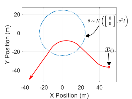
Figure 2: An optimal path computed for the first example, shown in red. In this example, the aircraft is only using Doppler shift measurements. The blue dashed circle is the 95% error ellipse of the prior distribution on $\theta$, which in this example represents the position of the vehicle target.

We consider a passive RF sensor that measures the Doppler frequency shift in the carrier frequency, denoted as ${\mathcal{F}}$, arising from the relative motion between transmitting vehicle and the receiver. Note that we do not need to decode the underlying transmission, as we are only tracking the carrier frequency. More details about the derivation of this, as well as other sensor models can be found in [1].

We assume in this paper the sensor produces conditionally independent measurements, each with a Gaussian distribution with mean $\mu_{\mathcal{F}}\left(\theta\right)$. While the mean vector depends on the parameter of interest, $\theta$, the covariance does not depend on $\theta$and is given as $\Sigma_{\mathcal{F}}$. This gives a closed form expression for $\left(\ref{eq:Inner Q(x;theta)}\right)$ for measurement ${\mathcal{F}}$, as

$$Q\left(x;\theta\right)=\left(\frac{\partial\mu_{\mathcal{F}}\left(\theta\right)}{\partial\theta}\right)^{\top}\Sigma_{\mathcal{F}}^{-1}\left(\frac{\partial\mu_{\mathcal{F}}\left(\theta\right)}{\partial\theta}\right),$$ (33)

where $\frac{\partial\mu_{\mathcal{F}}\left(\theta\right)}{\partial\theta}$ denotes the Jacobian matrix of $\mu_{\mathcal{F}}\left(\theta\right)$ [26]. To estimate the expectation and find the expression $\left(\ref{eq:Q(x)}\right)$, we choose a second-order Taylor series expansion. Let $Q_{ij}\left(x;\theta\right)$ denote the $i,j$-th element of the $\left(\ref{eq:Gaussian FIM}\right)$, and $\theta$ is a random variable with mean $\mu_{\theta}$ and covariance $\Sigma_{\theta}$. Then we approximate the element with a second order Taylor expansion as

$$Q_{ij}\left(x;\theta\right)\approx Q_{ij}\left(x;\mu_{\theta}\right)+\nabla Q_{ij}\left(x;\mu_{\theta}\right)^{\top}\left(\theta-\mu_{\theta}\right)$$

$$+\frac{1}{2}\left(\theta-\mu_{\theta}\right)^{\top}{\bf H}_{ij}\left(x;\mu_{\theta}\right)\left(\theta-\mu_{\theta}\right),$$

where ${\bf H}_{ij}\left(x;\theta\right)$ is the hessian matrix of $Q_{ij}\left(x;\theta\right)$ with respect to $\theta$. The expected value is then found as

$${\mathbb{E}}_{\theta}\left[Q_{ij}\left(x;\theta\right)\right]\approx Q_{ij}\left(x;\mu_{\theta}\right)+\frac{1}{2}\text{tr}\left(\Sigma_{\theta}{\bf H}_{ij}\left(x;\mu_{\theta}\right)\right).$$ (34)

The closed-form gradient $\frac{\partial\mu_{\mathcal{F}}\left(\theta\right)}{\partial\theta}$ in $\left(\ref{eq:Gaussian FIM}\right)$ are found from [1], while the Hessian values were found using the CasADI toolbox [27].

In the example the parameters to be estimated, $\theta$, consist of the $\left(X,Y\right)\in{\mathbb{R}}^{2}$ position of the target vehicle. The prior distribution of $\theta$ is given as

$$\theta\sim{\mathcal{N}}\left(\left[\begin{array}[]{c}0\\ 0\end{array}\right],\upsilon^{2}I\right),$$

where $\upsilon=10m$ is the standard deviation. The sensor measures the Doppler shifts with noise standard deviation of $\Sigma_{\mathcal{F}}=1$. The sensing aircraft is flying $1000\,m$ above the ground level where the target vehicle is located and the turn rate is limited with $\omega_{\text{max}}=0.05$ rad/s.

Figure 2 shows the optimal path from the initial condition of $X\left(0\right)=50\,m$, $Y\left(0\right)=-36.6\,m$, and $\psi\left(0\right)=-\pi$. The initial angle of $-\pi$ implies the tracking aircraft is moving from right to left initially at $t=0$. It can be seen in the figure that the optimal path begins with turning maneuvers before traveling straight along a ray extending outward from the center of the prior distribution of $\theta$. Conceptually, travel along this ray will give maximum variation in Doppler shift, but the early maneuvers are still necessary since multiple directions of measurements are required to fully localize using only Doppler measurements

Figure 3 shows a series of optimal paths generated with same initial conditions for $X\left(0\right)$ and $\psi\left(0\right)$, but with a variation in the initial condition, $Y\left(0\right)$. The vertical initial condition, $Y\left(0\right)$, were chosen uniformly from a range $\left[-50,50\right]$. While the trajectories are different quantitatively from that of Figure 2, they share the same qualitative properties of an initial maneuver to gain measurements in various directions before traveling away from the prior belief, on a ray extending directly from the center.

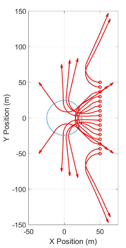
Figure 3: Here a series of optimal trajectories are shown in red from different starting locations, with each vehicle starting out moving from right to left. Same as in Fig. 2, the aircraft is only using Doppler shift measurements. The blue circle is the 95% error ellipse of the prior distribution on $\theta$.

7 Conclusion

We present a hybrid method of lines approach for solving a class of Hamilton–Jacobi PDEs that arise in the optimal placement of sensors. This method provides for robustness, where needed, in the $x$ subspace by using a classic grid approach with finite differencing. It avoids a grid in the $z$ subspace and hence scales well with the number of $z$ dimensions. We applied this to a trajectory optimization problem where the goal is to find the trajectory that minimizes the estimation error from the measurements collected along the calculated path. Future work includes investigating metrics other than logdet such as the trace of the inverse and studying if the hybrid method of lines approach can be generalized to a broader class of systems.

8 Hamiltonian Regularity Assumptions

Let $n$ be the dimension of the augmented state variable $\chi$, and denote by $\sigma:=\left(p,\lambda\right)^{\top}$, and with a slight abuse of notation note that ${\mathcal{H}}\left(s,\chi,\sigma\right)={\mathcal{H}}\left(s,x,z,\sigma\right)={\mathcal{H}}\left(s,x,z,p,\lambda\right)$ and vice versa. We introduce a set of mild regularity assumptions:

(H1)

The Hamiltonian

$$\left[0,t\right]\times{\mathcal{X}}\times{\mathcal{Z}}\times{\mathbb{R}}^{n}\ni\left(s,x,z,p,\lambda\right)\mapsto{\mathcal{H}}\left(s,x,z,p,\lambda\right)\in{\mathbb{R}}$$

is continuous.

(H2)

There exists a constant $c>0$ such that for all $\left(s,x,z\right)\in\left[0,t\right]\times{\mathcal{X}}\times{\mathcal{Z}}$ and for all $\sigma^{\prime},\sigma^{\prime\prime}\in{\mathbb{R}}^{n}$, the following inequalities hold

$$\left|{\mathcal{H}}\left(s,x,z,\sigma^{\prime}\right)-{\mathcal{H}}\left(s,x,z,\sigma^{\prime\prime}\right)\right|\leq\kappa_{1}\left(\chi\right)\left\|\sigma^{\prime}-\sigma^{\prime\prime}\right\|,$$

and

$$\left|{\mathcal{H}}\left(s,x,z,{\bf 0}\right)\right|\leq\kappa_{1}\left(\chi\right),$$

with $\kappa_{1}\left(\chi\right)=c\left(1+\left\|\chi\right\|\right)$.

(H3)

For any compact set $M\subset{\mathbb{R}}^{n}$ there exists a constant $C\left(M\right)>0$ such that for all $\chi^{\prime},\chi^{\prime\prime}\in M$ and for all $\left(s,\sigma\right)\in\left[0,t\right]\times{\mathbb{R}}^{n}$ the inequality holds

$$\left|{\mathcal{H}}\left(s,\chi^{\prime},\sigma\right)-{\mathcal{H}}\left(s,\chi^{\prime\prime},\sigma\right)\right|\leq\kappa_{2}\left(\sigma\right)\left\|\chi^{\prime}-\chi^{\prime\prime}\right\|;$$

with $\kappa_{2}\left(\sigma\right)=C\left(M\right)\left(1+\left\|\sigma\right\|\right)$.

(H4)

The terminal cost function

$${\mathbb{R}}^{n}\ni\chi\mapsto G\left(\chi\right)\in{\mathbb{R}},$$

is continuous.

Next we present an important theorem on the existence and uniqueness of viscosity solutions of the Hamilton–Jacobi equation.

Theorem 0.4 ([28, Theorem II.8.1, p. 70]).

Let assumptions $\left(H1\right)-\left(H4\right)$ hold. Then there exists a unique viscosity solution to $\left(\ref{eq:HJB Equation-1}\right)$.

9 Supporting Propositions

Proposition 0.5.

Let $\chi\in\mathcal{S}$, then

$$\frac{\partial}{\partial z}\xi\left(t;\chi,\bar{u}\left(\cdot\right)\right)=I.$$

Proof.

By assumption, the terminal point of the state trajectory $\zeta\left(t;\chi,\bar{u}\left(\cdot\right)\right)$ is differentiable with respect to initial condition $\chi\in\mathcal{S}$. Defining the Jacobin, for $s\in\left[0,t\right]$,

$$m\left(s\right):=\left[\begin{array}[]{cc}m_{xx}\left(s\right)&m_{x,z}\left(s\right)\\ m_{zx}\left(s\right)&m_{zz}\left(s\right)\end{array}\right]$$

$$=\left[\begin{array}[]{cc}\bar{\gamma}_{x}\left(s\right)&\bar{\gamma}_{z}\left(s\right)\\ \bar{\xi}_{x}\left(s\right)&\bar{\xi}_{z}\left(s\right)\end{array}\right]=\frac{\partial}{\partial\chi}\zeta\left(s;\chi,\bar{u}\left(\cdot\right)\right).$$

We have from [16, Chapter 5, Equation 3.23] that $m\left(t\right)$ satisfies the following matrix equation almost everywhere:

$$\begin{cases}\dot{m}\left(s\right)=\hat{f}_{\chi}\left(\bar{\zeta}\left(s;\chi,\bar{u}\left(\cdot\right)\right),\bar{u}\left(s\right)\right)m\left(s\right),&s\in\left[0,t\right],\\ m\left(0\right)=I.\end{cases}$$

From which the $m_{zz}$ partition is written as

$$\begin{cases}\dot{m}_{zz}\left(s\right)=\ell_{z}\left(\bar{\gamma}\left(s;\chi,\bar{u}\left(\cdot\right)\right)\right)m_{zz}\left(s\right),&s\in\left[0,t\right],\\ m_{zz}\left(0\right)=I.\end{cases}$$

Since $\ell$ does not depend on $z$, we have

$$\dot{m}_{zz}\left(s\right)=0,\,\forall s\in\left[0,t\right],$$

and the result follows. ∎

Matthew R. KirchnerThumbnail.jpg received his B.S. in Mechanical Engineering from Washington State University in 2007 and his M.S. in Electrical Engineering from the University of Colorado at Boulder in 2013. In 2007 he joined the Naval Air Warfare Center Weapons Division in the Navigation and Weapons Concepts Develop Branch and in 2012 transferred into the Physics and Computational Sciences Division in the Research and Intelligence Department, Code D5J1000. He is currently a Ph.D. candidate studying Electrical Engineering at the University of California, Santa Barbara. His research interests include level set methods for optimal control, differential games, and reachability; multi-vehicle robotics; nonparametric signal and image processing; and navigation and flight control. He was the recipient of a Naval Air Warfare Center Weapons Division Graduate Academic Fellowship from 2010 to 2012; in 2011 was named a Paul Harris Fellow by Rotary International and in 2021 was awarded a Robertson Fellowship from the University of California in recognition of an outstanding academic record. Matthew is a student member of the IEEE.

David Grimsmandavid.jpg is an Assistant Professor in the Computer Science Department at Brigham Young University. He completed BS in Electrical and Computer Engineering at Brigham Young University in 2006 as a Heritage Scholar, and with a focus on signals and systems. After working for BrainStorm, Inc. for several years as a trainer and IT manager, he returned to Brigham Young University and earned an MS in Computer Science in 2016. He then received his PhD in Electrical and Computer Engineering from UC Santa Barbara in 2021. His research interests include mulit-agent systems, game theory, distributed optimization, network science, linear systems theory, and security of cyberphysical systems.

João P. HespanhaJoao_Office_Ratio.jpg received his Ph.D. degree in electrical engineering and applied science from Yale University, New Haven, Connecticut in 1998. From 1999 to 2001, he was Assistant Professor at the University of Southern California, Los Angeles. He moved to the University of California, Santa Barbara in 2002, where he currently holds a Professor position with the Department of Electrical and Computer Engineering. Dr. Hespanha is the recipient of the Yale University’s Henry Prentiss Becton Graduate Prize for exceptional achievement in research in Engineering and Applied Science, the 2005 Automatica Theory/Methodology best paper prize, the 2006 George S. Axelby Outstanding Paper Award, and the 2009 Ruberti Young Researcher Prize. Dr. Hespanha is a Fellow of the IEEE and he was an IEEE distinguished lecturer from 2007 to 2013. His current research interests include hybrid and switched systems; multi-agent control systems; distributed control over communication networks (also known as networked control systems); the use of vision in feedback control; stochastic modeling in biology; and network security.

Jason R. Mardenjason.jpg is a professor in the Department of Electrical and Computer Engineering at the University of California, Santa Barbara. He received the B.S. degree in 2001 and the Ph.D. degree in 2007 (under the supervision of Jeff S. Shamma), both in mechanical engineering from the University of California, Los Angeles, where he was awarded the Outstanding Graduating Ph.D. Student in Mechanical Engineering. After graduating, he was a junior fellow in the Social and Information Sciences Laboratory at the California Institute of Technology until 2010 and then an assistant professor at the University of Colorado until 2015. He is a recipient of an ONR Young Investigator Award (2015), an NSF Career Award (2014), the AFOSR Young Investigator Award (2012), the SIAM CST Best Sicon Paper Award (2015), and the American Automatic Control Council Donald P. Eckman Award (2012). His research interests focus on game-theoretic methods for the control of distributed multiagent systems.