A Levenberg-Marquardt Method for Nonsmooth Regularized Least Squares

Abstract

We develop a Levenberg-Marquardt method for minimizing the sum of a smooth nonlinear least-squares term $f(x)=\tfrac{1}{2}\|F(x)\|_{2}^{2}$ and a nonsmooth term $h$. Both $f$ and $h$ may be nonconvex. Steps are computed by minimizing the sum of a regularized linear least-squares model and a model of $h$ using a first-order method such as the proximal gradient method. We establish global convergence to a first-order stationary point of both a trust-region and a regularization variant of the Levenberg-Marquardt method under the assumptions that $F$ and its Jacobian are Lipschitz continuous and $h$ is proper and lower semi-continuous. In the worst case, both methods perform $O(\epsilon^{-2})$ iterations to bring a measure of stationarity below $\epsilon\in(0,1)$. We report numerical results on three examples: a group-lasso basis-pursuit denoise example, a nonlinear support vector machine, and parameter estimation in neuron firing. For those examples to be implementable, we describe in detail how to evaluate proximal operators for separable $h$ and for the group lasso with trust-region constraint. In all cases, the Levenberg-Marquardt methods perform fewer outer iterations than a proximal-gradient method with adaptive step length and a quasi-Newton trust-region method, neither of which exploit the least-squares structure of the problem. Our results also highlight the need for more sophisticated subproblem solvers than simple first-order methods.

49J52, 65K10, 90C53, 90C56,

1 Introduction

We consider the problem

(1) $$\mathop{\textup{minimize}}_{x}\ f(x)+h(x),\qquad f(x)=\tfrac{1}{2}\|F(x)\|_{2}^{2},$$

where $F:\mathds{R}^{n}\to\mathds{R}^{m}$ is continuously differentiable and $h:\mathds{R}^{n}\to\mathds{R}$ is proper and lower semi-continuous; we allow $h$ to be nonsmooth and nonconvex. In practice, $f$ is often a data-misfit term while $h$ is a regularizer designed to promote desirable properties in the solution, such as sparsity. Numerous applications investigated in the nonsmooth regularized optimization literature actually have the structure (1), including basis pursuit denoising [14, 28], sparse factorization and dictionary learning [2], and sparse total least squares [30]. Yet nonsmooth numerical methods do not exploit the least-squares structure, nor accommodate general nonsmooth regularizers.

We describe two methods for (1): a quadratic regularization variant and trust-region variant inspired by the method of Levenberg [19] and Marquardt [21], denoted LM and LMTR respectively. Steps are computed by approximately minimizing simpler nonsmooth iteration-dependent Gauss-Newton-type models. Our algorithmic realizations utilize first-order methods, such as the proximal gradient method or the quadratic regularization method of Aravkin et al. [1], to solve the subproblems. The trust-region approach allows for any arbitrary trust-region norm, which, in practice, is influenced by nonconvex subproblem tractibility. For both algorithms, we establish global convergence in terms of an optimality measure describing achievable decrease by a single proximal gradient step. Additionally, we derive a worst-case complexity bound of $\mathcal{O}(1/\epsilon^{2})$ iterations to bring the stationarity measure below a tolerance of $\epsilon\in(0,1)$ for LM and LMTR, i.e., the presence of a nonsmooth term in the objective yields a complexity bound of the same order as in the smooth case.

We provide implementation details and illustrate the performance of our methods on several numerical examples, including basis pursuit denoise with group-lasso regularization, nonlinear support vector machine with $\ell_{1/2}^{1/2}$-norm regularization, and a sparse parameter estimation example taken from the Fitzhugh-Nagumo model of neuron firing. Our methods exhibit favorable performance under certain conditions with respect to previous work Aravkin et al. [1]. We additionally provide efficient, open-source software implementations of LM and LMTR as a package in the Julia language [3]. We find that exploiting the least-squares structure yields few LM and LMTR outer iterations, a well-known benefit in smooth optimization. The cost incurred is a large number of inner iterations, i.e, spent solving the subproblem. Thus, the results highlight the need for more sophisticated methods to minimize the sum of a linear least-squares term and a nonsmooth regularizer.

Related research

The present research is based on the framework laid out by Aravkin, Baraldi, and Orban [1]. The convergence and complexity of our trust-region Levenberg-Marquardt implementation follow directly from the general results of [1]. To the best of our knowledge, the trust-region literature does not explicitly cover the case of a nonlinear least-squares smooth objective with a nonsmooth regularizer other than a penalty term even though numerous applications exhibit that structure. See [13] for background and an extensive treatment.

A large portion of the literature focuses on $h$ convex and/or globally Lipschitz continuous, e.g., Cartis et al. [11], Grapiglia et al. [17] and references therein. We do not attempt to give a comprehensive account of that literature here as we focus on significantly weaker assumptions. While many methods exist in the first-order literature, e.g., [12], few can effectively utilize any significant curvature information. Proximal Newton methods [18] require solutions to nontrivial proximal operators and positive semi-definiteness of the Hessian. The small number of references that allow both $f$ and $h$ to be nonconvex that we are aware of include: Li and Lin [20], who design accelerations of the proximal gradient method under the assumption that $f+h$ is coercive; Bolte et al. [8] who design an alterating method for cases where $h(x)=h_{1}(x_{1})+h_{2}(x_{2})$ and $(x_{1},x_{2})$ is a partition of $x$; Stella et al. [26] who propose a linesearch limited-memory BFGS method named PANOC; Themelis et al. [27] who propose a nonmonotone linesearch proximal quasi-Newton method named ZeroFPR based on the forward-backward envelope; and Boţ et al. [9], who study a proximal method with momentum. The last three converge if $f+h$ satisfies the Kurdyka-Łojasiewicz (KŁ) assumption. Moreover, while all include (1) as a special case, few exploit any curvature information and none are specific to the least-squares structure. The algorithms presented here, like those of [1], require no such coercivity or KŁ  assumptions.

Notation

We use $\|\cdot\|$ to represent a generic, but fixed, norm on $\mathds{R}^{n}$ or $\mathds{R}^{m}$. The unit ball defined by that norm is $\mathbb{B}$, and $x+\Delta\mathbb{B}$ is the ball centered at $x$ of radius $\Delta>0$. For an integer $q\geq 1$, $\|\cdot\|_{q}$ is the $\ell_{q}$-norm and $\mathbb{B}_{q}$ is the unit ball in the $\ell_{q}$-norm. If $A\subseteq\mathds{R}^{n}$, $\chi(\cdot\mid A)$ is the indicator of $A$, i.e., the function whose value is $0$ if $x\in A$ and $+\infty$ otherwise. Unless otherwise noted, if $A$ is a matrix, $\|A\|$ denotes the spectral norm of $A$, i.e., its largest singular value. We use $J(x):\mathds{R}^{n}\to\mathds{R}^{n\times m}$ to denote the Jacobian of $F$ at $x$.

2 Background

Definition 2.1 (Limiting subdifferential).

Consider $\phi:\mathds{R}^{n}\rightarrow\overline{\mathds{R}}$ and $\bar{x}\in\mathds{R}^{n}$ with $\phi(\bar{x})<\infty$. We say that $v\in\mathds{R}^{n}$ is a regular subgradient of $\phi$ at $\bar{x}$, and we write $v\in\hat{\partial}\phi(\bar{x})$ if

$$\liminf_{x\to\bar{x}}\,\frac{\phi(x)-\phi(\bar{x})-v^{T}(x-\bar{x})}{\|x-\bar{x}\|_{2}}\geq 0.$$

The set of regular subgradients is also called the Fréchet subdifferential. We say that $v$ is a general subgradient of $\phi$ at $\bar{x}$, and we write $v\in\partial\phi(\bar{x})$, if there are sequences $\{x_{k}\}$ and $\{v_{k}\}$ such that

$$x_{k}\to\bar{x},\quad\phi(x_{k})\to\phi(\bar{x}),\quad v_{k}\in\hat{\partial}\phi(x^{k})\text{ and }\ v^{k}\to v.$$

The set of general subgradients is called the limiting subdifferential.

Proposition 2.2 (25, Theorem 10.1).

If $\phi:\mathds{R}^{n}\to\overline{\mathds{R}}$ is proper and has a local minimum at $\bar{x}$, then $0\in\hat{\partial}\phi(\bar{x})\subseteq\partial\phi(\bar{x})$. If $\phi$ is convex, the latter condition is also sufficient for $\bar{x}$ to be a global minimum. If $\phi=f+h$ where $f$ is continuously differentiable on a neighborhood of $\bar{x}$ and $h$ is finite at $\bar{x}$, then $\partial\phi(\bar{x})=\nabla f(\bar{x})+\partial h(\bar{x})$.

If $0\in\hat{\partial}\phi(\bar{x})$, we say that $\bar{x}$ is first-order stationary for $\phi$. Under our assumptions,

(2) $$x\text{ is first-order stationary for~{}\eqref{eq:nlls}}\quad\Longleftrightarrow\quad 0\in J{(x)}^{T}F(x)+\partial h(x).$$

The proximal gradient method [16] applied to a regularized objective $f(x)+h(x)$ where $f$ is differentiable is defined by the iteration

(3) $$x_{k+1}\in\mathop{\textup{prox}}_{\nu h}(x_{k}-\nu\nabla f(x_{k}))\qquad(k\geq 0),$$

where $\nu>0$ is a steplength and the proximal operator is defined as

(4) $$\mathop{\textup{prox}}_{\nu h}(y):=\mathop{\textup{argmin}}_{u}\tfrac{1}{2}\|u-y\|_{2}^{2}+\nu h(u).$$

Without further assumptions on $h$, (4) is a set that may be empty, or contain one or more elements. The iteration (3) has the following descent property

Lemma 2.3 (8, Lemma $2$).

Let $\nabla f$ be Lipschitz continuous with Lipschitz constant $L\geq 0$, $h$ be proper lower semi-continuous and $\inf h>-\infty$. Let $x_{k}\in\mathop{\textup{dom}}h$, $0<\nu<1/L$, and $x_{k+1}$ be defined according to (3). Then,

(5) $$(f+h)(x_{k+1})\leq(f+h)(x_{k})-\tfrac{1}{2}(\nu^{-1}-L)\|x_{k+1}-x_{k}\|_{2}^{2}.$$

3 Linear Least Squares

For fixed $\sigma\geq 0$ and $x\in\mathds{R}^{n}$, define

(6a) $$\varphi(s;x) :=\tfrac{1}{2}\|J(x)s+F(x)\|_{2}^{2},$$

(6b) $$\psi(s;x) \approx h(x+s)\quad\text{with}\quad\psi(0;x)=h(x),$$

(6c) $$m(s;x,\sigma) :=\varphi(s;x)+\tfrac{1}{2}\sigma\|s\|_{2}^{2}+\psi(s;x).$$

Consider the parametric problem and its optimal set

(7a) $$p(x,\sigma) :=\min_{s}\ m(s;x,\sigma)\leq\varphi(0;x)+\psi(0;x)=f(x)+h(x)$$

(7b) $$P(x,\sigma) :=\mathop{\textup{argmin}}_{s}\ m(s;x,\sigma).$$

The form of (7) is representative of a Levenberg-Marquardt subproblem for (1) in which $f$ and $h$ are modeled separately.

In particular, $\varphi(0;x)=f(x)$ and $\nabla_{s}\varphi(0;x)=\nabla f(x)$. We make the following additional assumption.

Model Assumption 3.1.

For any $x\in\mathds{R}^{n}$, $\psi(\cdot;x)$ is proper, lsc and prox-bounded, i.e., there exists $\lambda_{x}\in\mathds{R}_{+}\cup\{+\infty\}$ such that $\psi(\cdot;x)+\tfrac{1}{2}\lambda_{x}^{-1}\|\cdot\|_{2}^{2}$ is bounded below. In addition, $\psi(0;x)=h(x)$, and $\partial\psi(0;x)=\partial h(x)$.

In Model Assumption 3.1, we assume that our choice of $\lambda_{x}$ is the supremum of all possible choices, and we refer to it as the threshold of prox-boundedness of $\psi(\cdot;x)$. In particular, $\psi(\cdot;x)$ is bounded below if and only if $\lambda_{x}=+\infty$.

By Proposition 2.2, if $\sigma\geq\lambda_{x}^{-1}$,

$$s\in P(x,\sigma)\quad\Longrightarrow\quad 0\in\nabla\varphi(s;x)+\sigma s+\partial\psi(s;x).$$

We define

(8) $$\xi(x,\sigma):=(f+h)(x)-p(x,\sigma).$$

The following stationarity criterion follows directly from the definitions above.

Lemma 3.1.

Let Model Assumption 3.1 be satisfied and $\sigma\geq\lambda_{x}^{-1}$. Then $\xi(x,\sigma)=0\Longleftrightarrow 0\in P(x,\sigma)\Longrightarrow x$ is first-order stationary for (1). In addition, $x$ is first-order stationary for (1) if and only if $s=0$ is first-order stationary for (6c).

Proof 3.2.

Note first that $\xi(x,\sigma)=0\Longleftrightarrow p(x,\sigma)=(f+h)(x)=\varphi(0;x)+\psi(0;x)$, which occurs if and only if $0\in P(x,\sigma)$. Proposition 2.2 then implies $0\in\partial m(0;x,\sigma)=\nabla\varphi(0;x)+\partial\psi(0;x)$ and is equivalent to (2).

The next result states some properties of (7).

Proposition 3.3.

Let Model Assumption 3.1 be satisfied. $\mathop{\textup{dom}}p=\mathop{\textup{dom}}P=\mathop{\textup{dom}}\psi\times\{\sigma\mid\sigma\geq\lambda_{x}^{-1}\}$. In addition, for any $x\in\mathds{R}^{n}$,

1. $p(x,\cdot)$ is proper lsc and for each $\sigma>\lambda_{x}^{-1}$, $P(x,\sigma)$ is nonempty and compact;

2. if $\{\sigma_{k}\}\to\bar{\sigma}>\lambda_{x}^{-1}$ in such a way that $\{p(x,\sigma_{k})\}\to p(x,\bar{\sigma})$, and for each $k$, $s_{k}\in P(x,\sigma_{k})$, then $\{s_{k}\}$ is bounded and all its limit points are in $P(x,\bar{\sigma})$;

3. $p(x,\cdot)$ is continuous at any $\bar{\sigma}>\lambda_{x}^{-1}$ and $\{p(x,\sigma_{k})\}\to p(x,\bar{\sigma})$ holds in part 2 if $\bar{\sigma}>0$.

Proof 3.4.

Parts 1–2 follow from applying [25, Theorem $1.17$] by noting that (6c) is level-bounded in $s$ locally uniformly in $(x,\sigma)$ because $\psi(\cdot;x)+\tfrac{1}{2}\lambda_{x}^{-1}\|s\|_{2}^{2}$ is bounded and $\varphi(s;x)+\tfrac{1}{2}(\sigma-\lambda_{x}^{-1})\|s\|_{2}^{2}$ is level bounded in $s$ locally uniformy in $(x,\sigma)$. Part 3 also follows from [25, Theorem $1.17$] by noting that (6c) is continuous in $\sigma$ at any $\bar{\sigma}>\lambda_{x}^{-1}$.

By Proposition 3.3 part 3, $\xi(x,\cdot)$ is continuous at any $\bar{\sigma}>\lambda_{x}^{-1}$.

Although (6a) is a natural model of $f$ about $x$, convergence properties may be stated in terms of the simpler first-order model

(9a) $$\varphi_{1}(s;x) :=f(x)+\nabla f(x)^{T}s=\tfrac{1}{2}\|F(x)\|_{2}^{2}+{(J(x)^{T}F(x))}^{T}s,$$

(9b) $$m_{1}(s;x,\sigma) :=\varphi_{1}(s;x)+\tfrac{1}{2}\sigma\|s\|^{2}+\psi(s;x).$$

The first step of the proximal gradient method (3) applied to the minimization of both $\varphi(s;x)+\psi(s;x)$ and $\varphi_{1}(s;x)+\psi(s;x)$ with steplength $\nu>0$ is

(10) $$s_{1} \in\mathop{\textup{prox}}_{\nu\psi(\cdot;x)}(-\nu J{(x)}^{T}F(x))$$

$$=\mathop{\textup{argmin}}_{s}\ \tfrac{1}{2}\|s+\nu J{(x)}^{T}F(x)\|_{2}^{2}+\nu\psi(s;x)$$

$$=\mathop{\textup{argmin}}_{s}\ (J{(x)}^{T}F(x))^{T}s+\tfrac{1}{2}\nu^{-1}\|s\|_{2}^{2}+\psi(s;x)$$

$$=\mathop{\textup{argmin}}_{s}\ m_{1}(s;x,\nu^{-1}).$$

If $\nu^{-1}\geq\sigma$, then $m_{1}(s;x,\sigma)\leq m_{1}(s;x,\nu^{-1})$. Therefore, if $s_{1}$ results from (10), it also induces decrease in (9b).

In parallel to Lemma 3.1 and Proposition 3.3, we may define

(11a) $$p_{1}(x,\sigma) :=\min_{s}\ m_{1}(s;x,\sigma)\leq\varphi_{1}(0;s)+\psi(0;x)=f(x)+h(x)$$

(11b) $$P_{1}(x,\sigma) :=\mathop{\textup{argmin}}_{s}\ m_{1}(s;x,\sigma),$$

(11c) $$\xi_{1}(x,\sigma) :=(f+h)(x)-p_{1}(x,\sigma)\geq 0,$$

and we have the following results, stating corresponding properties of $p_{1}$ and $\xi_{1}$. The proofs replicate those in Proposition 3.3 and Lemma 3.5.

Lemma 3.5.

Let Model Assumption 3.1 be satisfied and $\sigma\geq\lambda_{x}^{-1}$. Then $\xi_{1}(x,\sigma)=0\Longleftrightarrow 0\in P_{1}(x,\sigma)\Longrightarrow x$ is first-order stationary for (1). In addition, $x$ is first-order stationary for (1) if and only if $s=0$ is first-order stationary for (9b).

Proposition 3.6.

Let Model Assumption 3.1 be satisfied. $\mathop{\textup{dom}}p_{1}=\mathop{\textup{dom}}P_{1}=\mathop{\textup{dom}}\psi\times\{\sigma\mid\sigma\geq\lambda_{x}^{-1}\}$. In addition, for any $x\in\mathds{R}^{n}$,

1. $p_{1}(x,\cdot)$ is proper lsc and for each $\sigma>\lambda_{x}^{-1}$, $P_{1}(x,\sigma)$ is nonempty and compact;

2. if $\{\sigma_{k}\}\to\bar{\sigma}>\lambda_{x}^{-1}$ in such a way that $\{p_{1}(x,\sigma_{k})\}\to p_{1}(x,\bar{\sigma})$, and for each $k$, $s_{k}\in P_{1}(x,\sigma_{k})$, then $\{s_{k}\}$ is bounded and all its limit points are in $P_{1}(x,\bar{\sigma})$;

3. $p_{1}(x,\cdot)$ is continuous at any $\bar{\sigma}>\lambda_{x}^{-1}$ and $\{p_{1}(x,\sigma_{k})\}\to p_{1}(x,\bar{\sigma})$ holds in part 2 if $\bar{\sigma}>0$.

Because $L=0$ for $\varphi_{1}$, Lemma 2.3 implies that the decrease achieved by $s_{1}$ is $(\varphi_{1}+\psi)(s_{1};x)\leq(\varphi_{1}+\psi)(0;x)-\tfrac{1}{2}\nu^{-1}\|s_{1}\|^{2}$, which can be rearranged as

(12) $$(f+h)(x)-(\varphi_{1}+\psi)(s_{1};x)\geq\tfrac{1}{2}\nu^{-1}\|s_{1}\|^{2}\geq\tfrac{1}{2}\sigma\|s_{1}\|^{2}.$$

In the special case where $\psi=0$, $s_{1}=-\nu^{-1}\nabla f(x)$, so that (12) reduces to

$$\xi_{1}(x,\sigma)\geq\xi_{1}(x,\nu^{-1})\geq f(x)-\varphi_{1}(s_{1};x)\geq\tfrac{1}{2}\sigma\nu^{-1}\|\nabla f(x)\|^{2}\geq\tfrac{1}{2}\sigma^{2}\|\nabla f(x)\|^{2},$$

which suggests that $\sigma^{-1}(\xi_{1}(x,\nu^{-1}))^{1/2}$ may be used as stationarity measure.

4 Nonlinear Least Squares

4.1 A regularization approach

We first examine the formulation of the method of Levenberg and Marquardt in which the model (6c) is employed to compute a step. Specifically, consider Algorithm 1. The step $s_{k}$ is computed by approximately minimizing (6c) in stage 7 but the quality of the step is measured without taking the regularization term $\tfrac{1}{2}\sigma_{k}\|s_{k}\|^{2}$ into account in stage 8. The subproblem step $s_{k}$ may be computed by continuing the iterations of the proximal gradient method initialized at $s_{k,1}$. This gives rise to one possible implementation of Algorithm 1.

Algorithm 1 Nonsmooth regularized Levenberg-Marquardt method.

1:Choose constants $0<\eta_{1}\leq\eta_{2}<1$ and $0<\gamma_{3}\leq 1<\gamma_{1}\leq\gamma_{2}$.

2:Choose $x_{0}\in\mathds{R}^{n}$ where $h$ is finite, $\sigma_{0}>0$, compute $F(x_{0})$ and $h(x_{0})$.

3:for $k=0,1,\dots$ do

4:     Choose a steplength $\nu_{k}<1/(\|J(x_{k})\|^{2}+\sigma_{k})$.

5:     Compute $s_{k,1}$ as defined in (10) and $\xi_{1}(x_{k},\nu_{k}^{-1})$ as defined in (11c).

6:     Define $m(s;x_{k},\sigma_{k})$ as in (6c).

7:     Compute an approximate solution $s_{k}$ of (7b).

8:     Compute the ratio

$$\rho_{k}:=\frac{f(x_{k})+h(x_{k})-(f(x_{k}+s_{k})+h(x_{k}+s_{k}))}{\varphi(0;x_{k})+\psi(0;x_{k})-(\varphi(s_{k};x_{k})+\psi(s_{k};x_{k}))}.$$

9:     If $\rho_{k}\geq\eta_{1}$, set $x_{k+1}=x_{k}+s_{k}$. Otherwise, set $x_{k+1}=x_{k}$.

10:     Update the regularization parameter according to

$$\sigma_{k+1}\in\begin{cases}[\gamma_{3}\sigma_{k},\,\sigma_{k}]&\text{ if }\rho_{k}\geq\eta_{2},\\ [\sigma_{k},\,\gamma_{1}\sigma_{k}]&\text{ if }\eta_{1}\leq\rho_{k}<\eta_{2},\\ [\gamma_{1}\sigma_{k},\,\gamma_{2}\sigma_{k}]&\text{ if }\rho_{k}<\eta_{1}.\end{cases}$$

11:end for

It may occur that $\sigma_{k}\leq\lambda_{x_{k}}^{-1}$. In such a case, $\psi(s_{k};x_{k})=-\infty$ so that the rules of extended arithmetic imply $\rho_{k}=0$, whether $h(x_{k}+s_{k})=+\infty$ or is finite. Thus $s_{k}$ will be rejected at stage 9 and $\sigma_{k+1}$ will be chosen larger than $\sigma_{k}$ at stage 10. After a finite number of such increases, $\sigma_{k}$ will exceed $\lambda_{x_{k}}^{-1}$ and a step with finite $\psi(s_{k};x_{k})$ will result.

Our main working assumption is the following.

Problem Assumption 4.1.

The residual $F$ and its Jacobian $J$ are bounded and Lipschitz continuous on $\Omega:=\{x\in\mathds{R}^{n}\mid(f+h)(x)\leq(f+h)(x_{0})\}$ and $h$ is proper and lower semi-continuous.

While Problem Assumption 4.1 is a strong demand on all of $\mathds{R}^{n}$ and, in particular, rules out the case of linear least squares, it is a common assumption in the convergence analysis of the Levenberg-Marquardt method. If $\Omega$ is a compact set, then $F$ is Lipschitz continuous on $\Omega$ if it is $\mathcal{C}^{1}$ on $\Omega$, and $J$ is Lipschitz continuous on $\Omega$ if $F$ is $\mathcal{C}^{2}$ on $\Omega$.

Under Problem Assumption 4.1, $\nabla f$ is Lipschitz continuous on $\Omega$, i.e., there exists $L>0$ such that

(13) $$|f(x+s)-(f(x)+\nabla f{(x)}^{T}s)|\leq\tfrac{1}{2}L\|s\|_{2}^{2}\quad\text{for all }x,\ x+s\in\Omega.$$

We emphasize that in what follows, knowledge of $L$, or an estimate thereof, is not required. Our next assumption on the model is the following.

Model Assumption 4.1.

There exists a constant $\kappa_{\textup{m}}>0$ such that for all $x$ and $s\in\mathds{R}^{n}$, $|(f+h)(x+s)-(\varphi+\psi)(s;x)|\leq\kappa_{\textup{m}}\|s\|^{2}$.

Model Assumption 4.1 is essentially an assumption on the nonsmooth part $\psi$ of the model. Indeed, (6a) and (13) combine to yield

$$|f(x+s)-\varphi(s;x)| \leq|f(x+s)-(f(x)+\nabla f{(x)}^{T}s)|+\tfrac{1}{2}\|J(x)s\|^{2}|$$

$$\leq\tfrac{1}{2}(L+\|J(x)\|^{2})\|s\|^{2}.$$

where we used the definition of $f(x)$, the identity $\nabla f(x)=J{(x)}^{T}F(x)$, and (13). Thus if $J$ is bounded on $\Omega$, we obtain

$$|f(x+s)-\varphi(s;x)|\leq\tfrac{1}{2}(L+\sup_{x\in\Omega}\|J(x)\|^{2})\|s\|^{2}.$$

In particular, Model Assumption 4.1 is satisfied with $\kappa_{\textup{m}}=\tfrac{1}{2}(L+\sup_{x\in\Omega}\|J(x)\|^{2})$ if we select $\psi(s;x):=h(x+s)$.

We make the following additional assumption and say that $\{\psi(\cdot;x_{k})\}$ is uniformly prox-bounded.

Model Assumption 4.2.

There exists $\lambda>0$ such that $\lambda_{x_{k}}\geq\lambda$ for all $k\in\mathds{N}$.

Model Assumption 4.2 is satisfied if $h$ itself is prox-bounded and we select $\psi(s;x_{k}):=h(x_{k}+s)$ at each iteration.

Our first result ensures that $\sigma_{k}$ is bounded above in Algorithm 1.

Theorem 4.1.

Let Problem Assumptions 4.1, 3.1, 4.1 and 4.2 be satisfied, and let

(14) $$\sigma_{\textup{succ}}:=\max(2\kappa_{\textup{m}}/(1-\eta_{2}),\,\lambda^{-1})>0.$$

If $x_{k}$ is not first-order stationary and $\sigma_{k}\geq\sigma_{\textup{succ}}$, then iteration $k$ is very successful and $\sigma_{k+1}\leq\sigma_{k}$.

Proof 4.2.

Let $s_{k}$ be the step computed at iteration $k$ of Algorithm 1. If $\sigma_{k}<\lambda_{x_{k}}^{-1}$, $\rho_{k}=0$ as explained above, $s_{k}$ is rejected and $\sigma_{k}$ is increased. Hence, we assume that $\sigma_{k}\geq\lambda^{-1}\geq\lambda_{x_{k}}^{-1}$. Because $x_{k}$ is not first-order stationary, $s_{k}\neq 0$. Because $s_{k}$ is an approximate solution of (7b), we must have

$$\varphi(0;x_{k})+\psi(0;x_{k})\geq\varphi(s_{k};x_{k})+\tfrac{1}{2}\sigma_{k}\|s_{k}\|^{2}+\psi(s_{k};x_{k})$$

and therefore,

(15) $$\varphi(0;x_{k})+\psi(0;x_{k})-(\varphi(s_{k};x_{k})+\psi(s_{k};x_{k}))\geq\tfrac{1}{2}\sigma_{k}\|s_{k}\|^{2}.$$

Model Assumption 4.1 and (15) combine to yield

$$|\rho_{k}-1|=\frac{|f(x_{k}+s_{k})+h(x_{k}+s_{k})-(\varphi(s_{k};x_{k})+\psi(s_{k};x_{k}))|}{\varphi(0;x_{k})+\psi(0;x_{k})-(\varphi(s_{k};x_{k})+\psi(s_{k};x_{k}))}\leq\frac{2\kappa_{\textup{m}}\|s_{k}\|^{2}}{\sigma_{k}\|s_{k}\|^{2}}.$$

After simplifying by $\|s_{k}\|^{2}$, we obtain $\sigma_{k}\geq\sigma_{\text{succ}}\Longrightarrow\rho_{k}\geq\eta_{2}$.

Note that Theorem 4.1 does not explicitly include Problem Assumption 4.1 in its assumptions, though it is likely to be required for Model Assumption 4.1 to hold.

Interestingly, Theorem 4.1 holds without assuming that the step $s_{k}$ satisfies a sufficient decrease condition. Upon examination of the proof, the reason turns out to be that any step that results in simple decrease in $m(s;\sigma,x)$ results in sufficient decrease in $\varphi(\cdot;x)+\psi(\cdot;x)$, independently of the method used to compute $s_{k}$.

Theorem 4.1 ensures existence of a constant $\sigma_{\max}>0$ such that

(16) $$\sigma_{k}\leq\sigma_{\max}:=\min(\sigma_{0},\gamma_{2}\sigma_{\textup{succ}})>0\quad\text{for all }k\in\mathds{N}.$$

Our next result concerns the situation where a finite number of successful iterations occur. The proof is almost identical to that of [13, Theorem $6.4.4$] and [1, Theorem $3.5$] and is omitted.

Theorem 4.3.

Let Problem Assumptions 4.1, 3.1 and 4.1 be satisfied. If Algorithm 1 only generates finitely many successful iterations, then $x_{k}=x^{*}$ for all sufficiently large $k$ and $x^{*}$ is first-order critical.

By Rockafellar and Wets [25, Theorem $1.25$], $p_{1}(x,\sigma)$ increases when $\sigma$ increases, and thus, $\xi_{1}(x,\sigma)$ decreases when $\sigma$ increases. Thus, it follows from (16) that

(17) $$\xi_{1}(x_{k},\sigma_{k})\geq\xi_{1}(x_{k},\sigma_{\max})\quad\text{for all }k\in\mathds{N}.$$

Lemma 3.1, (17) and the remarks at the end of Section 3 suggest using $\xi_{1}{(x_{k},\sigma_{\max})}^{\frac{1}{2}}$ as stationarity measure. Indeed, for given $\epsilon>0$, $\xi_{1}(x_{k},\sigma_{\max})\leq\epsilon/\sigma_{\max}\Longrightarrow\sigma_{k}\xi_{1}(x_{k},\sigma_{\max})\leq\epsilon$.

Because we must choose the steplength $\nu_{k}$ as in Step 4 of Algorithm 1, we compute $\xi_{1}(x_{k},\nu_{k}^{-1})$ rather than $\xi_{1}(x_{k},\sigma_{k})$. Concretely, for given $0<\theta<1$, we set

(18) $$\nu_{k}:=\theta/(\|J_{k}\|^{2}+\sigma_{k}).$$

Under Problem Assumption 4.1, there exists $\kappa_{J}>0$ such that $\|J(x)\|\leq\kappa_{J}$ for all $x\in\Omega$. Because Algorithm 1 only generates $x_{k}\in\Omega$, the above and (16) yield

(19) $$\nu_{k}\geq\theta/(\kappa_{J}^{2}+\sigma_{\max}):=\nu_{\min}>0\quad\text{for all }k\in\mathds{N}.$$

Therefore, $\nu_{k}^{-1}\leq\nu_{\min}^{-1}$ for all $k\geq 0$, and

(20) $$\xi_{1}(x_{k},\nu_{k}^{-1})\geq\xi_{1}(x_{k},\nu_{\min}^{-1})\quad\text{for all }k\in\mathds{N}.$$

For a stopping tolerance $\epsilon\in(0,\,1)$, we seek to determine $k(\epsilon)\in\mathds{N}$ such that

(21) $$\xi_{1}{(x_{k},\nu_{\min}^{-1})}^{\frac{1}{2}}>\epsilon\quad\text{for all }k<k(\epsilon)\quad\text{and}\quad\xi_{1}{(x_{k(\epsilon)},\nu_{\min}^{-1})}^{\frac{1}{2}}\leq\epsilon.$$

Define the sets

(22a) $$\mathcal{S} :=\{k\in\mathds{N}\mid\rho_{k}\geq\eta_{1}\},$$

(22b) $$\mathcal{S}(\epsilon) :=\{k\in\mathcal{S}\mid k<k(\epsilon)\},$$

(22c) $$\mathcal{U}(\epsilon) :=\{k\in\mathds{N}\mid k\not\in\mathcal{S}\text{ and }k<k(\epsilon)\}.$$

In order to conduct the complexity analysis, it is necessary to assume that the step computation at stage 7 of Algorithm 1 is related to $\xi_{1}(x_{k},\sigma_{k})$. We make the following assumption.

Step Assumption 4.1.

There exists $\kappa_{\textup{mdc}}\in(0,\,1)$ such that $s_{k}$ computed at stage 7 of Algorithm 1 satisfies

(23) $$\varphi(0;x_{k})+\psi(0;x_{k})-(\varphi(s_{k};x_{k})+\psi(s_{k};x_{k}))\geq\kappa_{\textup{mdc}}\xi_{1}(x_{k},\nu_{k}^{-1}).$$

Step Assumption 4.1 is similar to sufficient decrease conditions used in trust-region methods—see [13]. Aravkin et al. [1] provide a concrete use of such condition in a trust-region method for nonsmooth regularized optimization. Clearly, the sufficient decrease assumption is satisfied after a single step of the proximal gradient method applied to (6c). Hence, it is also satisfied at a minimizer of (6c). Thus, in step 7 of Algorithm 1, one strategy is to continue the proximal-gradient iterations until a stopping condition is attained.

The following results parallel those of Aravkin et al. [1], which are in turn inspired from those of Cartis et al. [11] and references therein.

Lemma 4.4.

Let Problem Assumptions 4.1, 3.1 and 4.1 be satisfied and $s_{k}$ be computed according to Step Assumption 4.1, where $\nu_{k}$ is chosen according to (18). Assume there are infinitely many successful iterations and that $f(x)+h(x)\geq{(f+h)}_{\textup{low}}$ for all $x\in\mathds{R}^{n}$. Then, for all $\epsilon\in(0,\,1)$,

(24) $$|\mathcal{S}(\epsilon)|\leq\frac{(f+h)(x_{0})-(f+h)_{\textup{low}}}{\eta_{1}\kappa_{\textup{mdc}}\epsilon^{2}}=O(\epsilon^{-2}).$$

Proof 4.5.

For $k\in\mathcal{S}(\epsilon)$, Step Assumption 4.1 and (20) imply

$$(f+h)(x_{k})-(f+h)(x_{k}+s_{k}) \geq\eta_{1}(\varphi(0;x_{k})+\psi(0;x_{k})-(\varphi(s_{k};x_{k})+\psi(s_{k};x_{k})))$$

$$\geq\eta_{1}\kappa_{\textup{mdc}}\xi_{1}(x_{k},\nu_{k}^{-1})$$

$$\geq\eta_{1}\kappa_{\textup{mdc}}\xi_{1}(x_{k},\nu_{\min}^{-1})$$

$$\geq\eta_{1}\kappa_{\textup{mdc}}\epsilon^{2}.$$

The rest of the proof mirrors that of [1, Lemma $3.6$].

Lemma 4.6.

Under the assumptions of Lemma 4.4,

(25) $$|\mathcal{U}(\epsilon)|\leq\frac{\log(\sigma_{\max}/\sigma_{0})}{\log(\gamma_{1})}+|\mathcal{S}(\epsilon)|\frac{|\log(\gamma_{3})|}{\log(\gamma_{1})}=O(\epsilon^{-2}).$$

Proof 4.7.

For each $k\in\mathcal{U}(\epsilon)$, $\sigma_{k+1}\geq\gamma_{1}\sigma_{k}$, while for each $k\in\mathcal{S}(\epsilon)$, $\sigma_{k+1}\geq\gamma_{3}\sigma_{k}$. Thus if $k(\epsilon)$ is the iteration for which (21) occurs for the first time,

$$\sigma_{0}\gamma_{1}^{|\mathcal{U}(\epsilon)|}\gamma_{3}^{|\mathcal{S}(\epsilon)|}\leq\sigma_{k(\epsilon)-1}\leq\sigma_{\max}.$$

Taking logarithms, we have

$$|\mathcal{U}(\epsilon)|\log(\gamma_{1})+|\mathcal{S}(\epsilon)|\log(\gamma_{3})\leq\log(\sigma_{\max}/\sigma_{0}).$$

Rearranging and recalling that $0<\gamma_{3}<1$ yields (25).

Combining Lemmas 4.4 and 4.6 yields the overall iteration complexity bound.

Theorem 4.8.

Under the assumptions of Lemma 4.4,

(26) $$|\mathcal{S}(\epsilon)|+|\mathcal{U}(\epsilon)|=O(\epsilon^{-2}).$$

Stated differently, Theorem 4.8 ensures that either $(f+h)(x_{k})\to-\infty$ or that $\liminf_{k\to\infty}\xi_{1}(x_{k},\nu_{\min}^{-1})=0$.

4.2 A trust-region approach

We now apply Algorithm $3.1$ of Aravkin et al. [1] to (1). We assume that each $f_{i}:\mathds{R}^{n}\to\mathds{R}$ is $\mathcal{C}^{1}$, so that their Problem Assumption $3.1$ is satisfied. A natural model for $f$ about $x$ is the Gauss-Newton model (6a), which satisfies $\varphi(0;x)=f(x)$ and $\nabla_{s}\varphi(0;x)=\nabla f(x)=J{(x)}^{T}F(x)$. The model $\psi(s;x)$ of $h(x+s)$ is required to satisfy the same Model Assumption 4.1, which holds provided $\nabla f$ is Lipschitz continuous or each $f_{i}$ is $\mathcal{C}^{2}$ with bounded Hessian. In Aravkin et al. [1, Algorithm $3.1$], the first proximal gradient step $s_{1}$ is computed by solving

(27) $$\mathop{\textup{minimize}}_{s} \tfrac{1}{2}\|F(x)\|_{2}^{2}+{(J{(x)}^{T}F(x))}^{T}s+\tfrac{1}{2}\nu^{-1}\|s\|^{2}+\psi(s;x)$$

$$\mathop{\textup{subject to}} \ \|s\|\leq\Delta,$$

i.e.,

$$s_{1}\in\mathop{\textup{prox}}_{\nu\psi(\cdot;x)+\chi(\cdot\mid\Delta\mathbb{B})}(-\nu J{(x)}^{T}F(x)),$$

where $0<\nu<1/(\|J(x)\|^{2}+\alpha^{-1}\Delta^{-1})$ for a preset constant $\alpha>0$. Subsequent steps continue the proximal gradient iterations to compute an approximate solution of

(28) $$\mathop{\textup{minimize}}_{s}\ \tfrac{1}{2}\|J(x)s+F(x)\|_{2}^{2}+\psi(s;x)\quad\ \mathop{\textup{subject to}}\|s\|\leq\min(\beta\|s_{1}\|,\,\Delta),$$

where $\beta\geq 1$. The above describes a trust-region variant of the method of Levenberg [19] and Marquardt [21] for regularized nonlinear least-squares problems. The assumption that $\psi(\cdot;x)$ is prox-bounded can be removed because $\psi(\cdot;x)+\chi(\cdot\mid\Delta\mathbb{B})$ is always bounded below, hence prox-bounded with $\lambda_{x}=\infty$. An approximate solution of (28) must satisfy Step Assumption 4.1 with $\xi_{1}(x,\sigma)$ replaced with

$$\hat{\xi}_{1}(\Delta;x,\nu):=f(x)+h(x)-\hat{p}_{1}(\Delta;x,\nu),$$

where $\hat{p}_{1}(\Delta;x,\nu)$ is the optimal value of (27).

Under the above assumptions, Aravkin et al. establish that the trust-region radius $\Delta$ never drops below the threshold

$$\Delta_{\min}:=\min\left(\Delta_{0},\,\hat{\gamma}_{1}\frac{\kappa_{\textup{mdc}}(1-\eta_{2})}{2\kappa_{\textup{m}}\alpha\beta^{2}}\right),$$

where $\Delta_{0}>0$ is the initial trust-region radius, $\hat{\gamma}_{1}\in(0,\,1)$ is the fraction by which $\Delta$ is reduced on rejected steps, $\eta_{2}\in(0,\,1)$ is the threshold above which $\Delta$ is increased on accepted steps, and $\kappa_{\textup{mdc}}$ and $\kappa_{\textup{m}}$ play similar roles as the constants of the same name in Model Assumptions 4.1 and 4.1.

Aravkin et al. use $\hat{\xi}_{1}(\Delta_{\min};x,\nu)$ as stationarity measure. They show that for any $\epsilon\in(0,\,1)$, the number of iterations necessary to achieve

$$\hat{\xi}_{1}(\Delta_{\min};x,\nu)^{\frac{1}{2}}\leq\epsilon$$

is $O(\epsilon^{-2})$ provided that $f+h$ is bounded below. We refer the reader to [1] for complete details.

5 Proximal operators

In Algorithm 1 or the algorithm of Section 4.2, a typical model of the nonsmooth term $h$ is $\psi(s;x):=h(x+s)$. If those algorithms are to use Aravkin et al.’s quadratic regularization method [1, Algorithm $6.1$] to compute a step, the latter will in turn form a model of $\psi(\cdot;x)$ at each iteration. In order to simplify notation, let $\psi_{k}(s):=\psi(s;x_{k})=h(x_{k}+s)$ be the model used at iteration $k$ of Algorithm 1 or the algorithm of Section 4.2.

5.1 General proximal operators

In Algorithm 1, the nonsmooth term in the objective of the subproblem is $\psi_{k}(s)$. The typical model about $s_{j}$ reduces to $\omega_{j}(t)=\psi_{k}(s_{j}+t)=h(x_{k}+s_{j}+t)$ and, instead of (30), the step computed is

(29) $$t_{j}\in\mathop{\textup{argmin}}_{t}\ \tfrac{1}{2}\nu^{-1}\|t-q\|^{2}+h(x_{k}+s_{j}+t).$$

The same change of variable as above yields

$$v_{j}\in\mathop{\textup{argmin}}_{v}\ \tfrac{1}{2}\nu^{-1}\|v-\bar{q}\|^{2}+h(v)=\mathop{\textup{prox}}_{\nu h}(\bar{q}),$$

whether $h$ is separable or not. Thus we obtain

$$t_{j}\in\mathop{\textup{prox}}_{\nu h}(\bar{q})-(x_{k}+s_{j}).$$

The nonsmooth term in the objective of the subproblem of the algorithm of Section 4.2 is $\psi_{k}(s)+\chi(s;\Delta_{k})$. About iterate $s_{j}$ of [1, Algorithm $6.1$], the user supplies a model $\omega_{j}(t):=\omega(t;s_{j})\approx\psi_{k}(s_{j}+t)+\chi(s_{j}+t\mid\Delta_{k}\mathbb{B})$, and the typical choice is $\omega_{j}(t)=\psi_{k}(s_{j}+t)+\chi(s_{j}+t\mid\Delta_{k}\mathbb{B})=h(x_{k}+s_{j}+t)+\chi(s_{j}+t\mid\Delta_{k}\mathbb{B})$. The step computed is $t_{j}\in\mathop{\textup{prox}}_{\nu\omega_{j}}(q)$ for certain fixed $\nu>0$ and $q\in\mathds{R}^{n}$, i.e.,

(30) $$t_{j}\in\mathop{\textup{argmin}}_{t}\ \tfrac{1}{2}\nu^{-1}\|t-q\|^{2}+h(x_{k}+s_{j}+t)+\chi(s_{j}+t\mid\Delta_{k}\mathbb{B}).$$

The change of variables $v:=x_{k}+s_{j}+t$ allows us to rewrite (30) as

(31) $$v_{j}\in\mathop{\textup{argmin}}_{v}\ \tfrac{1}{2}\nu^{-1}\|v-\bar{q}\|^{2}+h(v)+\chi(v-x_{k}\mid\Delta_{k}\mathbb{B}),$$

where $\bar{q}:=x_{k}+s_{j}+q$, from which we recover $t_{j}=v_{j}-(x_{k}+s_{j})$.

5.2 Separable shifted proximal operators

If $h$ is separable and the trust region is defined by the $\ell_{\infty}$-norm, the problem decomposes and the $i$-th component of $v_{j}$ is

(32) $$v_{j,i} \in\mathop{\textup{argmin}}_{v_{i}}\ \tfrac{1}{2}\nu^{-1}(v_{i}-\bar{q}_{i})^{2}+h_{i}(v_{i})+\chi(v_{i}-x_{k,i}\mid[-\Delta_{k},\Delta_{k}])$$

$$=\mathop{\textup{argmin}}_{v_{i}}\ \tfrac{1}{2}\nu^{-1}(v_{i}-\bar{q}_{i})^{2}+h_{i}(v_{i})+\chi(v_{i}\mid[x_{k,i}-\Delta_{k},x_{k,i}+\Delta_{k}]).$$

Two situations may occur. In the first situation, $x_{k,i}-\Delta_{k}<v_{j,i}<x_{k,i}+\Delta_{k}$, so that $v_{j,i}\in\mathop{\textup{prox}}_{\nu h_{i}}(\bar{q}_{i}),$ i.e.,

$$t_{j,i}\in\mathop{\textup{prox}}_{\nu h_{i}}(\bar{q}_{i})-(x_{k,i}+s_{j,i}).$$

In the second situation, at least one unconstrained solution lies outside of $[x_{k,i}-\Delta_{k},x_{k,i}+\Delta_{k}]$, so that constrained global minima of (32) are either one or both bounds, and/or unconstrained local minima that lie between the bounds.

When $h$ is convex, the constrained solution is the feasible point nearest the unique unconstrained global solution, i.e.,

$$v_{j,i}\in\mathop{\textup{proj}}_{[x_{k,i}-\Delta_{k},x_{k,i}+\Delta_{k}]}(\mathop{\textup{prox}}_{\nu h_{i}}(\bar{q}_{i})),$$

i.e.,

$$t_{j,i}\in\mathop{\textup{proj}}_{[x_{k,i}-\Delta_{k},x_{k,i}+\Delta_{k}]}(\mathop{\textup{prox}}_{\nu h_{i}}(\bar{q}_{i}))-(x_{k,i}+s_{j,i}).$$

Example 5.1 ($\ell_{1/2}^{1/2}$ pseudonorm).

Consider $\psi(s)=\|s\|_{1/2}^{1/2}=\sum_{j}|s_{j}|^{1/2}$. When the trust-region bounds are inactive, Cao et al. [10] express the solution of (32) as

$$v_{j,i}=\begin{cases}\phantom{-}\tfrac{2}{3}|\bar{q}_{i}|\left(1+\cos\left(\tfrac{2}{3}\pi-\tfrac{2}{3}\mu_{\lambda}(\bar{q}_{i})\right)\right)&\quad\phantom{|}\bar{q}_{i}\phantom{|}>p(\lambda)\\ \phantom{-}0&\quad|\bar{q}_{i}|\leq p(\lambda)\\ -\tfrac{2}{3}|\bar{q}_{i}|\left(1+\cos\left(\tfrac{2}{3}\pi-\tfrac{2}{3}\mu_{\lambda}(\bar{q}_{i})\right)\right)&\quad\phantom{|}\bar{q}_{i}\phantom{|}<-p(\lambda)\end{cases}$$

where

$$\mu_{\lambda}(\bar{q}_{i})\coloneqq\arccos\left(\frac{\lambda}{4}\left(\frac{|\bar{q}_{i}|}{3}\right)^{-3/2}\right),\qquad p(\lambda)\coloneqq\frac{54^{1/3}}{4}(2\lambda)^{2/3}.$$

When the trust-region constraint is active, Cao et al. [10] state that the above yields the inflection points of (32). We simply check the inflection points as well as the bounds. If the inflection points are within the bounds, we choose the minimum; if not, we select the minimum value of the cost function at the bounds.

5.3 Nonseparable shifted proximal operators for convex $h$

In this section we consider examples of nonseparable shifted proximal operators. The starting point is (31) where we assume that $h$ is closed, proper, and convex. We rewrite

$$\chi(v-x\mid\Delta\mathbb{B})=\sup_{z}\,\langle v-x,z\rangle-\sigma_{\Delta\mathbb{B}}(z),$$

where we write $x$ and $\Delta$ instead of $x_{k}$ and $\Delta_{k}$ for simplicity, and where the support function

$$\sigma_{\Delta\mathbb{B}}(z):=\sup_{d}\,\langle d,z\rangle+\chi(d\mid\Delta\mathbb{B}).$$

We substitute into (31) and obtain the saddle point problem

(33) $$\min_{v}\sup_{z}\,\tfrac{1}{2}\nu^{-1}\|v-\bar{q}\|^{2}+h(v)+\langle v-x,z\rangle-\sigma_{\Delta\mathbb{B}}(z).$$

The objective of (33) is convex in $v$ and concave in $z$. The saddle-point conditions can be written

$$0 \in\nu^{-1}(v-\bar{q})+\partial h(v)+z=\nu^{-1}(v-(\bar{q}-\nu z))+\partial h(v)$$

$$0 \in v-x-\partial\sigma_{\Delta\mathbb{B}}(z).$$

The first condition implies that $v\in\mathop{\textup{prox}}_{\nu h}(\bar{q}-\nu z)$. By convexity of $h$, $v$ is unique so that we are left with

(34) $$0\in v-x-\partial\sigma_{\Delta\mathbb{B}}(z),\quad\text{where}\quad\mathop{\textup{prox}}_{\nu h}(\bar{q}-\nu z)=\{v\}.$$

5.3.1 Special case: $\ell_{2}$-norm

For $h(\cdot):=\lambda\|\cdot\|_{2}$,

(35) $$\mathop{\textup{prox}}_{\nu\lambda\|\cdot\|_{2}}(y)=\begin{cases}0&\text{ if }\|y\|\leq\nu\lambda\\ \left(1-\frac{\nu\lambda}{\|y\|_{2}}\right)y&\text{ if }\|y\|>\nu\lambda\end{cases}.$$

We now show how to solve (31) by converting (34) to a scalar root finding problem. For given $z$, let

$$\zeta=\zeta(z):=\|\bar{q}-\nu z\|_{2}.$$

There are two possibilities.

Case A: If $\zeta\leq\nu\lambda$, (35) yields

$$\mathop{\textup{prox}}_{\nu\lambda\|\cdot\|_{2}}(\bar{q}-\nu z)=\{v\}=\{0\}.$$

The optimal value of (31) in this case is $\tfrac{1}{2}\nu^{-1}\|\bar{q}\|^{2}$.

Case B: If $\zeta>\nu\lambda$, (35) yields

(36) $$\mathop{\textup{prox}}_{\nu\lambda\|\cdot\|_{2}}(\bar{q}-\nu z)=\{v\}=\left\{\left(1-\frac{\nu\lambda}{\zeta}\right)(\bar{q}-\nu z)\right\},$$

and (34) becomes

$$0 \in x-\left(1-\frac{\nu\lambda}{\zeta}\right)(\bar{q}-\nu z)+\partial\sigma_{\Delta\mathbb{B}}(z)$$

$$=(\zeta-\nu\lambda)\frac{\nu}{\zeta}\left(z-\left(\frac{1}{\nu}\bar{q}-\frac{\zeta}{\nu(\zeta-\nu\lambda)}x\right)\right)+\partial\sigma_{\Delta\mathbb{B}}(z),$$

which we interpret as

(37) $$z=z(\zeta):=\mathop{\textup{prox}}_{\frac{\zeta}{\nu(\zeta-\nu\lambda)}\sigma_{\Delta\mathbb{B}}}\left(\frac{1}{\nu}\bar{q}-\frac{\zeta}{\nu(\zeta-\nu\lambda)}x\right).$$

Recall that [6, Theorem $6.46$]

(38) $$\mathop{\textup{prox}}_{\alpha\sigma_{\Delta\mathbb{B}}}(y)=y-\alpha\mathop{\textup{proj}}_{\Delta\mathbb{B}}(\alpha^{-1}y),\quad(\alpha>0).$$

Therefore, the projection into $\Delta\mathbb{B}$ must be computable. In our implementation, we use $\mathbb{B}=\mathbb{B}_{\infty}$.

We may now search for $\zeta$ such that

(39) $$g(\zeta):=\zeta-\|\bar{q}-\nu z(\zeta)\|_{2}=0.$$

Because projections into convex sets are Lipschitz continuous, so is $g$ over $(\nu\lambda,+\infty)$.

Since (31) is strongly convex, there is a unique solution, and so $g$ has at most one root such that $\zeta>\nu\lambda$. Any such root of $g$ yields $v$ given by (36) and $z(\zeta)$ given by (37) that jointly satisfy (34). If $g$ has no such root, the Case A must occur.

The combination of (37) and (38) yields

(40) $$\bar{q}-\nu z(\zeta)=\frac{\zeta}{\zeta-\nu\lambda}\left[x+\mathop{\textup{proj}}_{\Delta\mathbb{B}}\left(\frac{\zeta-\nu\lambda}{\zeta}\bar{q}-x\right)\right].$$

As $\zeta\uparrow\infty$, $(\zeta-\nu\lambda)/\zeta\uparrow 1$, and by continuity, the term between square brackets in (40) converges to $x+\mathop{\textup{proj}}_{\Delta\mathbb{B}}(\bar{q}-x)$. Therefore, $\|\bar{q}-\nu z(\zeta)\|_{2}\to\|x+\mathop{\textup{proj}}_{\Delta\mathbb{B}}(\bar{q}-x)\|_{2}$ and for sufficiently large $\zeta$, we must have $g(\zeta)>0$.

To study $g(\zeta)$ as $\zeta\downarrow\nu\lambda$, we consider several mutually-exclusive cases.

1. If $x\not\in\Delta\mathbb{B}$, then, $\mathop{\textup{proj}}_{\Delta\mathbb{B}}(-x)\neq-x$. As $\zeta\downarrow\nu\lambda$, $(\zeta-\nu\lambda)/\zeta\downarrow 0$, and by continuity, the term between square brackets converges to $x+\mathop{\textup{proj}}_{\Delta\mathbb{B}}(-x)\neq 0$. Therefore, $\|\bar{q}-\nu z(\zeta)\|_{2}\to\infty$ and for sufficiently small $\zeta$, we must have $g(\zeta)<0$.

2. Consider next the case where $x\in\mathop{\textup{int}}\Delta\mathbb{B}$. For $\zeta$ sufficiently close to $\nu\lambda$,

   (41) $$\mathop{\textup{proj}}_{\Delta\mathbb{B}}\left(\frac{\zeta-\nu\lambda}{\zeta}\bar{q}-x\right)=\frac{\zeta-\nu\lambda}{\zeta}\bar{q}-x,$$

   and $\bar{q}-\nu z(\zeta)=\bar{q}$, i.e., $z(\zeta)=0$. In this case,

   1. if $\|\bar{q}\|_{2}>\nu\lambda$, then $g(\zeta)<0$ for $\zeta$ close enough to $\nu\lambda$,

   2. if $\|\bar{q}\|_{2}\leq\nu\lambda$, then $g(\zeta)>0$ for all $\zeta>\nu\lambda$;

3. If $\|x\|_{\infty}=\Delta$ and $\mathop{\textup{proj}}_{\Delta\mathbb{B}}(\bar{q}-x)=-x$, then $\mathop{\textup{proj}}_{\Delta\mathbb{B}}(\alpha\bar{q}-x)=-x$ for any $\alpha>0$. In this case, the term between square brackets in (40) is always zero, and $\bar{q}-\nu z(\zeta)=0$. Thus for all $\zeta>\nu\lambda$, $g(\zeta)=\zeta>0$.

4. If $\|x\|_{\infty}=\Delta$ but $\mathop{\textup{proj}}_{\Delta\mathbb{B}}(\bar{q}-x)\neq-x$, there are two possible situations. Either the ray $\alpha\bar{q}-x$ intersects $\mathop{\textup{int}}\Delta\mathbb{B}$, or it does not. If it does, (41) occurs for all $\zeta$ sufficiently close to $\nu\lambda$, $\bar{q}-\nu z(\zeta)=\bar{q}$, and cases 2a–2b apply. If it does not, we have from Lipschitz continuity that

   $$\left\|x+\mathop{\textup{proj}}_{\Delta\mathbb{B}}\left(\frac{\zeta-\nu\lambda}{\zeta}\bar{q}-x\right)\right\|_{2}\!=\left\|\mathop{\textup{proj}}_{\Delta\mathbb{B}}\left(\frac{\zeta-\nu\lambda}{\zeta}\bar{q}-x\right)-\mathop{\textup{proj}}_{\Delta\mathbb{B}}(-x)\right\|_{2}\!\leq\frac{\zeta-\nu\lambda}{\zeta}\|\bar{q}\|_{2}.$$

   Thus, $\|\bar{q}-\nu z(\zeta)\|_{2}\leq\|\bar{q}\|_{2}$, and

   1. if $\|\bar{q}\|_{2}>\nu\lambda$, then $g(\zeta)\geq\zeta-\|\bar{q}\|_{2}>0$ for $\zeta>\|\bar{q}\|_{2}$, and so there may exist a root in $(\nu\lambda,\|\bar{q}\|_{2}]$. By (40), and the fact that $\|y\|_{2}\leq\sqrt{n}\|y\|_{\infty}$ for all $y$, we also have

      $$\|\bar{q}\ -\nu z(\zeta)\|_{2}\leq\frac{\zeta}{\zeta-\nu\lambda}\left(\|x\|_{2}+\left\|\mathop{\textup{proj}}_{\Delta\mathbb{B}}\left(\frac{\zeta-\nu\lambda}{\zeta}\bar{q}-x\right)\right\|_{2}\right)\leq\frac{(\|x\|_{2}+\Delta\sqrt{n})\zeta}{\zeta-\nu\lambda},$$

      so that $g(\zeta)>0$ for $\zeta>\nu\lambda+2\Delta\sqrt{n}$. Thus, the search interval may potentially be reduced to $(\nu\lambda,\min(\nu\lambda+\|x\|_{2}+\Delta\sqrt{n},\|\bar{q}\|_{2})]$.

   2. if $\|\bar{q}\|\leq\nu\lambda$, then $g(\zeta)>0$ for all $\zeta>\nu\lambda$.

Thus, in cases 1 and 2a, a root is guaranteed to exist in $(\nu\lambda,+\infty)$ and can be found by a bisection method. The upper bound may be found by observing that (40) implies

$$\|\bar{q}-\nu z(\zeta)\|\leq\frac{\zeta}{\zeta-\nu}(\|x\|+\Delta),$$

so that

$$g(\zeta)=\zeta-\|\bar{q}-\nu z(\zeta)\|\geq\zeta-\frac{\zeta}{\zeta-\nu\lambda}(\|x\|+\Delta),$$

and $g(\zeta)>0$ as soon as $\zeta>\|x\|+\Delta+\nu\lambda$.

In case 1, a lower bound follows by applying the reverse triangle inequality to (40):

$$\|\bar{q}-\nu z(\zeta)\|\geq\frac{\zeta}{\zeta-\nu\lambda}(\|x\|-\Delta),$$

so that $g(\zeta)<0$ as soon as $\zeta<\nu\lambda+\|x\|-\Delta$.

In case 2a, the lower bound is simply $\|\bar{q}\|$.

In cases 2b, 3 and 4b, there can be no root in $(\nu\lambda,+\infty)$ and Case A must occur.

Only case 4a requires a root search, with or without sign change. If no root exists in the search interval, Case A must occur.

5.3.2 Special case: Group lasso

The group lasso penalty is a sum of $\ell_{2}$-norms of subvectors:

$$R_{g}(x)=\sum_{i}\|x_{[i]}\|_{2},$$

where the $x_{[i]}$ partition $x$ into non-overlapping groups. The proximal operator of $R_{g}$ consists in applying (35) to each subvector:

(42) $$\mathop{\textup{prox}}_{\lambda R_{g}}(z)_{[i]}=\left(1-\frac{\lambda}{\|z_{[i]}\|_{2}}\right)_{+}z_{[i]}.$$

Thus, the strategy of the previous section may be applied to each group.

6 Implementation and numerical experiments

Our implementation of Algorithm $3.1$ of [1] and Algorithm 1 for (1) employs Aravkin, Baraldi, and Orban’s quadratic regularization method, named R2, to compute a step. R2 may be viewed as an implementation of the proximal gradient method with adaptive step size. The trust-region variant uses $\Delta_{0}=1$, terminates the outer iterations as soon as $\xi(\Delta_{k};x_{k},\nu_{k})^{1/2}<\epsilon_{a}+\epsilon_{r}\,\xi_{1,0}^{1/2}$, where $\epsilon_{a}>0$ and $\epsilon_{r}>0$ are an absolute and a relative tolerance, and $\xi_{1,0}$ is the value of $\xi_{1}$ observed at the first iteration. A round of inner iterations terminates as soon as

(43) $$\hat{\xi}_{1}(x_{k}+s,\hat{\sigma}_{k})\leq\begin{cases}10^{-1}&\text{if }k=0,\\ \max(\epsilon,\min(10^{-1},\xi_{1}(x_{k},\sigma_{k})/10))&\text{if }k>0,\end{cases}$$

where $\hat{\sigma}_{k}$ and $\hat{\xi}_{1}$ are the regularization parameter and first-order stationarity measure used inside R2. In Algorithm 1, we use $\sigma_{0}=0.01$, and we terminate the outer iterations as soon as $\xi_{1}(x_{k},\sigma_{k})^{1/2}<\epsilon$ for a tolerance $\epsilon>0$ because $\sigma_{\max}$ is unknown. The inner iterations stop in the same manner as (43). All algorithms are implemented in the Julia language [7] version $1.8$ as part of the RegularizedOptimization.jl package [3]. The shifted proximal operators are implemented in the ShiftedProximalOperators.jl package [5], while test problems are in the RegularizedProblems.jl package [4]. By contrast with the numerical results of Aravkin et al. [1], test cases are explicitly implemented as nonlinear least-squares problems, with access to the residual $F(x)$ and its Jacobian, and not simply the gradient of $f(x):=\tfrac{1}{2}\|F(x)\|_{2}^{2}$. Jacobian-vector and transposed-Jacobian-vector products are either implemented manually or computed via forward [24] and reverse [23] automatic differentiation, respectively.

We perform comparisons with R2 and with the quasi-Newton trust-region method of Aravkin et al. [1], named TR, and which does not exploit the structure of (1). The trust region is defined in $\ell_{\infty}$-norm and the quadratic model uses a limited-memory SR1 Hessian approximation with memory $5$. In all experiments, we use $\psi(s;x):=h(x+s)$.

A direct comparison between the four methods is difficult because LM and LMTR do not utilize the same gradient; they instead take Jacobian-vector and transposed-Jacobian-vector products. To provide a meaningful comparison, in the tables below, we state: 1) the number of objective (or residual) evaluations; 2) the number of gradient evaluations (for R2 and TR) ; 3) the number of transposed-Jacobian-vector products (for LM and LMTR), listed under gradient evaluations; 4) the solve time in seconds. Our rationale is as follows. LM and LMTR pass a model to R2 whose objective evaluation requires one $Jv$, and whose gradient uses a $Jv$ and a $J^{T}v$. Note however that the latter $Jv$ can be cached and reused. Thus, R2 requires one $Jv$ at each iteration, and additionally one $J^{T}v$ at each successful iteration.

In the figures, we plot descent as a function of residual/objective evaluations.

The summary of the numerical results below is that exploiting the least-squares structure results in a large reduction in outer iterations. However, solving the subproblem with a first-order method such as R2 consumes many $J^{T}v$. Our experiments thus highlight the need for more sophisticated subproblem solvers dedicated to (6c) and (28).

6.1 Group LASSO

In the group-LASSO problem, we observe noisy data from a linear system $b=Ax_{T}+\varepsilon$, where $A\in\mathds{R}^{m\times n}$ has orthonormal rows, and $x_{T}$ is segmented into $g$ groups with every element in that group set to one of $\{-1,0,1\}$. The group-LASSO problem is given by

(44) $$\min_{x}\tfrac{1}{2}\|Ax-b\|_{2}^{2}+\lambda\|x\|_{1,2},$$

where $h(x)=\|x\|_{1,2}=\sum_{i=1}^{g}\|x_{[i]}\|_{2}$, i.e., the sum of the $\ell_{2}$-norm of the groups. The groups consisting of all zeros are labeled as “inactive”, whereas the groups set to $\pm 1$ are “active”. We let $m=512$, $n=200$ and $\lambda=10^{-2}$. We designate $g=5$ such groups of possible 16 (each with 32 elements) to be “active”. The noise $\varepsilon\sim\mathcal{N}(0,0.01)$. Thus (44) has the form (1), where $F(x)=Ax-b$. We set the absolute and relative exit tolerances to be $10^{-4}$ each. The number of subproblem iterations is capped at 100 for each outer iteration.

Figure 1 shows the solutions of each algorithm, and Table 2 reports the statistics. All algorithms arrive at approximately the same solution. R2 requires the most function evaluations whereas the others require about the same. Table 2 suggests that a tradoff exists between the number of proximal operator evaluations and the number of gradient/Jacobian-vector evaluations. TR takes many proximal iterations, whereas LMTR and LM take far fewer. This tradeoff is further exemplified in the next test cases.

Table 1: Group-LASSO (44) statistics for R2, TR, LM, and LMTR, and $h(x)=\|x\|_{1,2}$. The $\#\nabla f$ is the number of $J^{T}v$ for LM and LMTR.

Alg	$f(x)$	$h(x)$	$(f+h)(x)$	$\|x-x_{T}\|_{2}$	# $f$	# $\nabla f$	# $\mathop{\textup{prox}}$	$t$ (s)
R2	0.00	0.26	0.27	0.45	113	67	113	0.02
TR	0.00	0.26	0.27	0.47	17	17	339	2.56
LM	0.00	0.26	0.27	0.46	10	647	265	0.05
LMTR	0.00	0.26	0.27	0.46	5	327	130	0.98

(a) Signal: R2

(b) Signal: TR

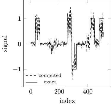
(c) Signal: LM

(d) Signal: LMTR

Figure 1: Group-LASSO (44) solutions with R2, TR, LM, and LMTR with $h=\lambda\|\cdot\|_{1,2}$.

We additionally plot descent history in Figure 4a. The plots are roughly similar, with the trust region methods TR and LMTR performing the best.

6.2 Nonlinear support vector machine

We now solve an image recognition problem of the form (1), where

(45) $$F(x)=\mathbf{1}-\tanh(b\odot\langle A,x\rangle),\quad\mathbf{1}=[1,\ldots,1]^{T},$$

$A\in\mathds{R}^{m\times n}$, $n=784$ is the vectorized image size, the number of images is $m=13007$ in the training set and $m=2163$ in the test set, and $\odot$ denotes the elementwise product between vectors. We wish to use this nonlinear SVM to classify digits of the MNIST dataset as either 1 or 7, with all other digits removed. We additionally impose the condition that the support is sparse, and therefore use $h(x)=\|x\|_{1/2}^{1/2}$ as a regularizer. Hence, our overall problem is

(46) $$\min_{x}\ \tfrac{1}{2}\|\mathbf{1}-\tanh(b\odot\langle A,x\rangle)\|^{2}+\lambda\|x\|_{1/2}^{1/2}$$

with $\lambda=10^{-1}$. We initialize the problem at $x=\mathbf{1}^{n}$ so that approximately 50% of the data is misclassified. We set the stopping tolerances again to $10^{-4}$ and the maximum number of inner iterations to $100$.

Figure 2 shows the solution map of each algorithm, which can be interpreted as the pixels most important in determining whether the image is indeed a 1 or 7. All algorithms produce a sparse solution; only about  8% of pixels in the support vector are nonzero. The problem is large and nonconvex; hence, the final solutions share pixels but altogether, they are different. This can be seen in Table 4, which reports the statistics. R2 again requires the most function evaluations. TR requires about 10 times more than LM and LMTR. We again observe that a tradoff exists between number of proximal operator evaluations and the number of gradient/Jacobian-vector evaluations. Here, proximal operator evaluations are cheaper than gradient or $Jv$ evaluations, so wallclock time is higher for LM and LMTR.

We plot descent history against number of function/residual iterations in Figure 4b. Here we can see LM and LMTR performing the best in terms of descent.

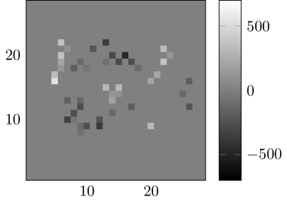
(a) Signal: R2

(b) Signal: TR

(c) Signal: LM

(d) Signal: LMTR

Figure 2: Nonlinear SVM (46) solutions with R2, TR, LM, LMTR.

Table 3: Nonlinear SVM (46) statistics for R2, TR, LM, and LMTR. Training/test error is with respect to the $\ell_{2}$-norm.

Alg	$f$	$h$	$f+h$	(Train, Test)	# $f$	# $\nabla f$	# $\mathop{\textup{prox}}$	$t$ (s)
R2	57.11	66.28	123.39	(99.80, 99.35)	1359	1085	1359	18.99
TR	49.80	72.37	122.17	(99.83, 99.26)	267	171	10478	6.62
LM	54.36	65.86	120.21	(99.83, 99.35)	23	3567	1276	24.98
LMTR	49.43	68.26	117.69	(99.81, 99.12)	24	3925	1420	44.32

6.3 FitzHugh-Nagumo inverse problem

The problem has the form (1), with $F:\mathds{R}^{5}\to\mathds{R}^{2n+2}$ defined as $F(x)=(v(x)-\bar{v}(\bar{x}),w(x)-\bar{w}(\bar{x}))$, where $v(x)=(v_{1}(x),\ldots,v_{n+1}(x))$ and $w(x)=(w_{1}(x),\ldots,w_{n+1}(x))$ are sampled values of discretized functions $V(t;x)$ and $W(t;x)$ satisfying the FitzHugh [15] and Nagumo et al. [22] model for neuron activation

(47) $$\frac{\mathrm{d}V}{\mathrm{d}t}=(V-V^{3}/3-W+x_{1})x_{2}^{-1},\quad\frac{\mathrm{d}W}{\mathrm{d}t}=x_{2}(x_{3}V-x_{4}W+x_{5}),$$

parametrized by $x$. The sampling is defined by a discretization of the time interval $t\in[0,\,20]$ and initial conditions $(V(0),W(0))=(2,0)$. The data $(\bar{v}(x),\bar{w}(x))$ is generated by solving (47) with $\bar{x}=(0,0.2,1,0,0)$, which corresponds to a simulation of the Van der Pol [29] oscillator. In our experiments, we use $n=100$ and solve

(48) $$\min_{x}\,\tfrac{1}{2}\|F(x)\|_{2}^{2}+\lambda\|x\|_{1},$$

where $h(x)=\lambda\|x\|_{1}$ with $\lambda=10$ to enforce sparsity in the parameters. Our absolute stopping criteria is $10^{-2}$, whereas our the relative stopping criteria is set to $10^{-4}$.

The solution found by each solver is given in Table 6 TR has the correct nonzero parameters, but the values are farther off. The corresponding simulations are shown in Figure 3; each method is able to fit the data.

Table 5: Final parameters for the FH problem (48) found by R2, TR, LM, and LMTR.

True	R2	TR	LM	LMTR
0.00	0.00	0.00	0.00	0.00
0.20	0.26	0.33	0.25	0.25
1.00	0.84	0.70	0.86	0.85
0.00	0.00	0.00	0.00	0.00
0.00	0.00	0.00	0.00	0.00

(a) Simulation: R2

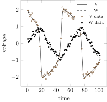
(b) Simulation: TR

(c) Simulation: LM

(d) Simulation: LMTR

Figure 3: Simulation of the FH problem (48) solutions found by R2, TR, LM, LMTR.

Table 8 reports the statistics for each algorithm, which exhibit the same pattern of results as before. The final objective values are fairly similar. LMTR uses the smallest amount of objective evaluations, whereas LM has a harder time solving (48). Because the gradient of the smooth term in (48) is not Lipschitz continuous, we had to set a $\sigma_{\min}$ for both R2 and LM, which increased iteration count. Similar to the SVM example, we can see that LM and LMTR take more time than TR, which again stems from proximal operators being much cheaper to compute than $Jv$ products for this example. Notably, TR seems to fit the data worse but attain a lower value of the regularizer.

Table 7: Statistics for the FH problem (48) for R2, TR, LM, and LMTR.

Alg	$f$	$h$	$f+h$	$\|x-x_{T}\|_{2}$	# $f$	# $\nabla f$	# $\mathop{\textup{prox}}$	$t$ (s)
R2	1.24	10.91	12.15	1.58	4230	3428	4230	40.40
TR	1.87	10.31	12.17	1.93	134	77	2452	0.67
LM	1.20	11.03	12.23	1.55	101	4236	1402	20.17
LMTR	1.20	11.02	12.22	1.55	32	2006	741	10.50

Finally, Fig. 4c shows descent of our objective function value against objective function iteration. LMTR again performs the best, whereas LM and TR were similar in this metric. This again enunciates the tradeoff between objective, gradient, and proximal operator expense. Expensive proximal evaluations would be the limiting factor in TR and R2; one can think of Total Variation regularization as a test case, since the proximal operator is itself a minimization problem.

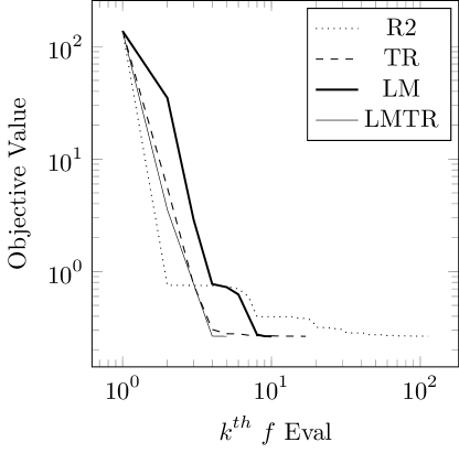
(a) Group-Lasso

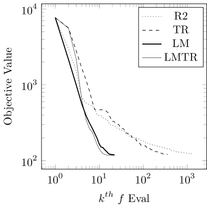
(b) SVM

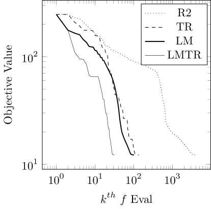
(c) FH

Figure 4: Objective decrease per objective or residual evaluation.

7 Discussion

Similarly to smooth optimization, exploiting the least-squares structure of $f$ can decrease significantly the number of outer iterations. The challenge highlighted by our numerical results, which is the subject of ongoing research, is to either identify a closed-form minimizer of (6c) for relevant choices of $\psi$, or to devise methods that can produce a higher-quality step than R2 with fewer transposed-Jacobian-vector products. As long as the subproblem solver yields a step satisfying Step Assumption 4.1, our convergence properties and worst-case complexity bounds are guaranteed to hold. Thus, any improvement in the step computation mechanism will immediately translate into a more efficient solver overall. In ongoing research, we are exploring other improvements, including inexact evaluations of $f$ and $\nabla f$, nonmonotone methods, and inexact evaluation of proximal operators.

References

- Aravkin et al. [2022] A. Aravkin, R. Baraldi, and D. Orban. A proximal quasi-Newton trust-region method for nonsmooth regularized optimization. SIAM J. Optim., (2):900–929, 2022.
- Bach et al. [2012] F. Bach, R. Jenatton, J. Mairal, and G. Obozinski. Optimization with Sparsity-Inducing Penalties, volume 4 of Foundations and Trends in Machine Learning. now publishers, 2012.
- Baraldi and Orban [2022a] R. Baraldi and D. Orban. RegularizedOptimization.jl: Algorithms for regularized optimization. https://github.com/JuliaSmoothOptimizers/RegularizedOptimization.jl, February 2022a.
- Baraldi and Orban [2022b] R. Baraldi and D. Orban. RegularizedProblems.jl: Test cases for regularized optimization. https://github.com/JuliaSmoothOptimizers/RegularizedProblems.jl, February 2022b.
- Baraldi and Orban [2022c] R. Baraldi and D. Orban. ShiftedProximalOperators.jl: Proximal operators for regularized optimization. https://github.com/JuliaSmoothOptimizers/ShiftedProximalOperators.jl, February 2022c.
- Beck [2017] A. Beck. First Order Methods in Optimization. SIAM, Philadelphia, USA, 2017.
- Bezanson et al. [2017] J. Bezanson, A. Edelman, S. Karpinski, and V. B. Shah. Julia: A fresh approach to numerical computing. SIAM Rev., 59(1):65–98, 2017.
- Bolte et al. [2014] J. Bolte, S. Sabach, and M. Teboulle. Proximal alternating linearized minimization for nonconvex and nonsmooth problems. Math. Program., (146):459––494, 2014.
- Boţ et al. [2016] R. I. Boţ, E. R. Csetnek, and S. László. An inertial forward–backward algorithm for the minimization of the sum of two nonconvex functions. EURO J. Comput. Optim., (4):3–25, 2016.
- Cao et al. [2013] W. Cao, J. Sun, and Z. Xu. Fast image deconvolution using closed-form thresholding formulas of lq (q = 12, 23) regularization. Journal on visual communication and image representation, 24(1), 2013.
- Cartis et al. [2011] C. Cartis, N. I. M. Gould, and Ph. L. Toint. On the evaluation complexity of composite function minimization with applications to nonconvex nonlinear programming. SIAM J. Optim., 21(4):1721–1739, 2011.
- Combettes and Pesquet [2011] P. L. Combettes and J.-C. Pesquet. Proximal splitting methods in signal processing. In Fixed-point algorithms for inverse problems in science and engineering, pages 185–212. Springer, 2011.
- Conn et al. [2000] A. R. Conn, N. I. M. Gould, and Ph. L. Toint. Trust-Region Methods. Number 1 in MOS-SIAM Series on Optimization. SIAM, Philadelphia, USA, 2000.
- Donoho [2006] D. L. Donoho. Compressed sensing. IEEE T. Inform. Theory, 52(4):1289–1306, 2006.
- FitzHugh [1955] R. FitzHugh. Mathematical models of threshold phenomena in the nerve membrane. B. Math. Biophys., 17(4):257–278, 1955.
- Fukushima and Mine [1981] M. Fukushima and H. Mine. A generalized proximal point algorithm for certain non-convex minimization problems. Int. J. Syst. Sci., 12(8):989–1000, 1981.
- Grapiglia et al. [2016] G. Grapiglia, J. Yuan, and Y. Yuan. Nonlinear stepsize control algorithms: Complexity bounds for first- and second-order optimality. J. Optim. Theory and Applics., (171):980––997, 2016.
- Lee et al. [2014] J. D. Lee, Y. Sun, and M. A. Saunders. Proximal Newton-type methods for minimizing composite functions. SIAM J. Optim., 24(3):1420–1443, 2014.
- Levenberg [1944] K. Levenberg. A method for the solution of certain problems in least squares. Q. Appl. Math., (2):164–168, 1944.
- Li and Lin [2015] H. Li and Z. Lin. Accelerated proximal gradient methods for nonconvex programming. In Proceedings of the 28th International Conference on Neural Information Processing Systems - Volume 1, NIPS’15, pages 379–387, Cambridge, MA, USA, 2015. MIT Press.
- Marquardt [1963] D. W. Marquardt. An algorithm for least-squares estimation of nonlinear parameters. Journal of the Society for Industrial and Applied Mathematics, 11(2):431–441, 1963.
- Nagumo et al. [1962] J. Nagumo, S. Arimoto, and S. Yoshizawa. An active pulse transmission line simulating nerve axon. Proceedings of the IRE, 50(10):2061–2070, 1962.
- Revels [2022] J. Revels. Reverse mode automatic differentiation for Julia. https://github.com/JuliaDiff/ReverseDiff.jl, 2022.
- Revels et al. [2016] J. Revels, M. Lubin, and T. Papamarkou. Forward-mode automatic differentiation in Julia, 2016. https://arxiv.org/abs/1607.07892.
- Rockafellar and Wets [1998] R. Rockafellar and R. Wets. Variational Analysis, volume 317. Springer Verlag, 1998.
- Stella et al. [2017] L. Stella, A. Themelis, P. Sopasakis, and P. Patrinos. A simple and efficient algorithm for nonlinear model predictive control. In 2017 IEEE 56th Annual Conference on Decision and Control (CDC), pages 1939–1944, 2017.
- Themelis et al. [2018] A. Themelis, L. Stella, and P. Patrinos. Forward-backward envelope for the sum of two nonconvex functions: Further properties and nonmonotone linesearch algorithms. SIAM J. Optim., 28(3):2274–2303, 2018.
- Tibshirani [1996] R. Tibshirani. Regression shrinkage and selection via the lasso. J. Roy. Statist. Soc. Ser. B, 58(1):267–288, 1996.
- Van der Pol [1926] B. Van der Pol. Lxxxviii. On “relaxation-oscillations”. The London, Edinburgh, and Dublin Philosophical Magazine and Journal of Science, 2(11):978–992, 1926.
- Zhu et al. [2011] H. Zhu, G. Leus, and G. B. Giannakis. Sparsity-cognizant total least-squares for perturbed compressive sampling. IEEE T. Signal Proces., 59(5):2002–2016, 2011.