Diffusion in Phase Space as a Tool to Assess Variability of Vertical Centre-of-Mass Motion During Long-Range Walking

Abstract

When a Hamiltonian system undergoes a stochastic, time-dependent anharmonic perturbation, the values of its adiabatic invariants as a function of time follow a distribution whose shape obeys a Fokker-Planck equation. The effective dynamics of the body’s centre-of-mass during human walking is expected to represent such a stochastically perturbed dynamical system. By studying, in phase space, the vertical motion of the body’s centre-of-mass of 25 healthy participants walking for 10-minutes at spontaneous speed, we show that the distribution of the adiabatic invariant is compatible with the solution of a Fokker-Planck equation with constant diffusion coefficient. The latter distribution appears to be a promising new tool for studying the long-range kinematic variability of walking.

I Introduction

Action-angle coordinates $(I_{\alpha},\theta^{\alpha})$, with $\alpha=1,\dots,n\,$, are of central importance in the study of deterministic classical systems with finitely many degrees of freedom. A time-independent integrable Hamiltonian may indeed be formulated as a separable function of the action variables only: $H=\sum^{n}_{i=\alpha}H_{0\alpha}(I_{\alpha})\,$. The equations of motion for such a system read (Landau and Lifchitz, 1988, Ch. 45):

$$\dot{I}_{\alpha}=-\frac{\partial H}{\partial\theta^{\alpha}}=0,\quad\dot{\theta}^{\alpha}=\frac{\partial H}{\partial I_{\alpha}}=:\omega_{\alpha}\;.$$ (1)

The action variables are constants of the motion and therefore $\omega_{\alpha}$ is also constant, implying that the angle coordinates read $\theta^{\alpha}=\omega_{\alpha}\,t+\theta^{\alpha}_{0}\,$ where $\omega_{\alpha}=\frac{2\pi}{T_{\alpha}}\,$ and $T_{\alpha}$ is the period of the motion in the plane $(I_{\alpha},\theta^{\alpha})$. Since the Kolmogorov-Arnold-Moser theorem (see Kolmogorov (1954); Arnol’d (1963); Möser (1962) and Dumas (2014) for a historical overview) and the work of Nekhoroshev Nekhoroshev (1971, 1977), the action-angle variables have proven to be the most useful for the study of stability of dynamical systems, including chaotic systems. We now restrict our formalism to systems with $n=1$, whose sole degrees of freedom consist in the pair $(I,\theta)\,$.

Suppose that $H$ depends on a function $\lambda(t)\,$. The action variable $I$ then becomes time-dependent and is called an adiabatic invariant. On the one hand, if $\lambda$ changes slowly during the typical period of a cycle, then the adiabatic invariant also changes slowly: $\dot{I}\sim\dot{\lambda}$ Landau and Lifchitz (1988); Henrard (1998); Jose and Saletan (1998). On the other hand, if $\lambda$ is a perturbative stochastic noise, the adiabatic invariant also becomes randomly time-dependent and the deviation from its average value remains perturbative. Detailed demonstrations and bounds for the deviation may be found in Khas’minskiĭ (1966); Cogburn and Ellison (1992). Moreover, for a Hamiltonian $H(I,\lambda(t))$ with perturbative stochastic noise $\lambda(t)$, it has been shown that the density $\rho(I,t)$ of the values of the adiabatic invariant as a function of time obeys a Fokker-Planck equation Bazzani et al. (1994, 1995); Bazzani and Beccaceci (1998). The latter phenomenon is a diffusion process in phase space. Besides its intrinsic interest, such a formalism has already found an important application in plasma physics, where it allows to relax standard simplifying assumptions and describe the problem in a less model-dependent way Kominis et al. (2010). The Fokker-Planck equation has also been recently applied to the study of robustness in gene expression Degond et al. (2020).

Biomechanical models of voluntary rhythmic movements in humans (of which walking has been studied most extensively) may also benefit from the above results. Such movements are quasi-periodic because of physiological noise, which prevents an individual from being in the same invariant state during repeated movements. The resulting variability has motivated many studies of human gait, most of which rely on the computation of nonlinear indices to assess variability (Hurst exponent, fractal dimension, etc.). We refer the interested reader to the pioneering works Hausdorff et al. (1995, 1997) and to Stergiou (2016); Ravi et al. (2020) for recent reviews. To our knowledge, the variability of gait has never been studied by assessing the shape and time evolution of the distribution $\rho(I,t)$. In the present work, we will show that that the distribution $\rho(I,t)$ in human walking indeed obeys a Fokker-Planck equation, i.e. that diffusion in phase space is experimentally observable in walking. Biomechanical models can then inherit the advantages of this formalism.

Our paper is structured as follows. In section II, diffusion in phase space and its use in modelling human walking is proposed. Then, in section III, the experimental setup is presented and numerical results are given in section IV. Finally, in section V, the results are discussed and concluding remarks are given.

II Diffusion in phase space

II.1 Generalities

Let us consider a one-dimensional Hamiltonian $H_{0}(I)$, where $I$ and $\theta$ are the action and angle coordinates, respectively. Suppose that a time-dependent stochastic perturbation is added to $H_{0}$ and that the latter Hamiltonian satisfies the stability assumptions underlying the Nekhoroshev theorem Nekhoroshev (1971, 1977). The total Hamiltonian $H$ may be written as follows:

$$H=H_{0}(I)+\epsilon\ \xi(t)\ {\cal V}(I,\theta)\;,$$ (2)

where $0<\epsilon\ll 1$, and where $\xi(t)$ is a stochastic noise with vanishing mean value. Under the dynamics controlled by $H$, the action variable becomes time-dependent and the deviation from the initial value $I_{0}$ is of order $\sqrt{\epsilon}\,$ up to a time of order $1/\epsilon\,$ or even better Khas’minskiĭ (1966); Cogburn and Ellison (1992). More precisely, $|I(t)-I_{0}|=O(\sqrt{\epsilon})$ and a time-dependent density distribution $\rho(I,t)$ of the values of the adiabatic invariant can be associated with its time evolution $I(t)\,$. As shown and illustrated in Bazzani et al. (1994, 1995); Bazzani and Beccaceci (1998), the density distribution $\rho(I,t)$ obeys a particular Fokker-Planck equation given by

$$\partial_{t}\rho=\partial_{I}(D(I)\partial_{I}\rho)\;,$$ (3)

where the function $D(I)\,$ is called the diffusion function. Considering the Fourier decomposition ${\cal V}(I,\theta)=\sum_{k}{\cal V}_{k}(I)\,{\rm e}^{ik\theta}$ of the perturbation function that appears in the Hamiltonian, the following expression is obtained Bazzani and Beccaceci (1998) for the diffusion function:

$$D(I)=\frac{\epsilon^{2}}{2}\sum_{k}k^{2}|{\cal V}_{k}(I)|^{2}\tilde{\phi}(k\omega)\;,$$ (4)

where $\tilde{\phi}(\nu)$ is the noise spectral density, i.e. $\tilde{\phi}(\nu)=\int^{+\infty}_{-\infty}\phi(u)\cos(\nu u)\,du$ with the autocorrelation function

$$\phi(u)=\lim_{T\to+\infty}\frac{1}{T}\int^{T}_{0}\xi(t)\xi(t+u)\,du\;.$$ (5)

Two particular cases can be highlighted. First, when $H=(\omega+\epsilon\,\xi(t))I\,$, only the $k=0$ mode ${\cal V}_{0}$ is nonzero and $D=0$. There is no diffusion in a pure harmonic oscillator with randomly perturbed frequency Bazzani et al. (1994). Second, in the case of constant diffusion coefficient, the normalised solution of (3) on the interval $I\in[0,+\infty[$ with boundary conditions $\rho(I,0)=\delta(I-I_{0})\,\Theta(t)\,$, $\Theta$ being the Heaviside step function, and $\rho(0,t)=0=\lim_{I\to+\infty}\rho(I,t)$, may be obtained:

$$\rho(I,t)=\Theta(t)\ \frac{{\rm e}^{-\frac{(I-I_{0})^{2}}{4Dt}}-{\rm e}^{-\frac{(I+I_{0})^{2}}{4Dt}}}{\sqrt{4\pi Dt}\ {\rm erf}\left(\frac{I_{0}}{\sqrt{4Dt}}\right)}=\Theta(t)\ \frac{{\rm e}^{-\frac{(I-I_{0})^{2}}{4Dt}}}{\sqrt{4\pi Dt}}\ \frac{1-{\rm e}^{-\frac{I\,I_{0}}{Dt}}}{{\rm erf}\left(\frac{I_{0}}{\sqrt{4Dt}}\right)}\;.$$ (6)

The normalisation is such that $\int^{+\infty}_{0}\rho(I,t)\,dI=\Theta(t)$. From now on, we will be interested in the second case of a constant but non-vanishing diffusion fonction.

We refer the interested reader to Risken and Haken (1989) for a general discussion of the construction of solutions of the Fokker-Planck equation, and to Fa (2005); Lin and Ho (2012) for explicit solutions with non-constant and nonzero diffusion and drift coefficients.

II.2 Application to human walking

It is known that the vertical displacement of the body’s centre-of-mass (COM) during human bipedal walking at spontaneous speed is compatible with a simple, spring-mass-like, model, see for example the famous work Cavagna et al. (1976). It is therefore tempting to model the vertical motion of the COM by the harmonic oscillator Hamiltonian $H_{0}=\frac{1}{2}(P^{2}+\omega^{2}Q^{2})=\omega\,I\,$, where $P$ and $Q$ are the vertical momentum and position of the COM, respectively. By definition, and assuming the standard relation $P\propto\dot{Q}\,$, one has

$$I=\frac{1}{2\pi}\oint_{\Gamma}P\,dQ=\frac{T\overline{E_{c}}}{\pi}\;,$$ (7)

with $\Gamma$ a cycle in phase space, $T$ the duration of the cycle and $\overline{E_{c}}$ the averaged kinetic energy over $\Gamma\,$.

Some phenomena suggest that the inclusion of other terms, at least in the perturbation, is necessary to obtain a more realistic model. First, the minimum (maximum) of the potential energy and the maximum (minimum) of kinetic energy are not reached at exactly the same time: a time shift of about 3 % of the gait cycle duration is observed Cavagna and Legramandi (2020). Such a feature requires a time-dependent correction to be added. Second, the Hamiltonian $H_{0}$ corresponds to a linearised pendulum only in the limiting case of small amplitudes. Anharmonic corrections should be added. The interested reader will find in Whittington and Thelen (2008) a more explicit model of the pendulum in which the potential term is nonlinear, and in Brizard (2013) a computation of action-angle variables for the fully non-linear pendulum with Hamiltonian $H_{0}=\frac{P^{2}}{2}+1-\cos Q$. Third, the parameters of the model ($\omega$ in our case) must have some time-dependent variability due to physiological noise; the state of a complex system like the human body is not identical from one gait cycle to another.

In view of the above discussion, a Hamiltonian of the form (2) in which $H_{0}$ is not a pure harmonic oscillator seems to be a relevant model of the vertical COM dynamics in action-angle formalism. As far as the perturbation $H_{1}(I,\theta)=\epsilon\ \xi(t)\ {\cal V}(I,\theta)$ is concerned, we will consider the simplest nontrivial ansatz with a constant but non-vanishing diffusion coefficient $D\,$. Referring to (4), this implies that all the functions ${\cal V}_{k}(I)$ are constant so that $H_{1}(I,\theta)$ only depends on the angle variable $\theta\,$. It does not depend on the total amount of action or energy in the system but only on time through the stochastic noise $\xi(t)$ and on the position in the cycle through ${\cal V}(\theta)\,$. Therefore, we assume that the influence of physiological noise on walking is related to the position in the gait cycle and not to the total action or the averaged kinetic energy of the walker – recall that $I\sim\overline{E_{c}}$. Consequently, Eq. (3) with a nonzero diffusion coefficient yields the heat equation

$$\partial_{t}\rho=D\,\partial^{2}_{I}\rho\;,$$ (8)

and the diffusion of the adiabatic invariant should be observable experimentally.

III Experimental setup

III.1 Protocol

The protocol was validated by the Academic Ethical Committee Brussels Alliance for Research and Higher Education (B200-2021-123). Participants were healthy students recruited in the physiotherapy department of the Haute-Ecole Louvain en Hainaut (Montignies-sur-Sambre, Belgium). After being informed about the study, each participant signed an informed consent form.

Biometric data were first collected (age, weight, height), as well as information on the wearing of orthopaedic insoles and the participant’s medical and trauma history. The participant is then asked to put on a tight-fitting garment. In order for his or her movements to be recorded by a Vicon optoelectronic system (Vicon Motion Systems Ltd, Oxford Metrics, Oxford, UK) consisting of 8 cameras (Vero v.2 .2) with a recording frequency of 120 Hz, 4 reflective markers with a diameter of 14 mm were placed on the participant according the Plug-In-Gait model (Oxford Metrics, Oxford, United Kingdom): Left Anterior Superior Iliac Spine [LASI], Right Anterior Superior Iliac Spine [RASI], Left Posterior Superior Iliac Spine [LPSI], and Left Posterior Superior Iliac Spine [RPSI].

After this preparatory phase, the participant walked for 3 minutes on an N-Mill instrumented treadmill (Motekforce Link, The Netherlands). The purpose of this familiarisation phase is to determine the participant’s spontaneous walking speed. No other data were recorded during this period. After the walking speed was recorded, the participant walked on the treadmill for 10 minutes at the previously determined spontaneous speed. During these 10 minutes, the average number of steps per minute was measured by the treadmill and the three-dimensional trajectory of the 4 markers, $\vec{x}_{a}(t)$, was recorded by the Vicon system using the Vicon Nexus software (v.2.7.1, Oxford Metrics, Oxford, UK).

The general characteristics of our participants are listed in Table 1. We note that an initial analysis of these data was presented in a recent work Buisseret et al. (2022), in which we showed that an adiabatic invariant exists in the vertical motion of the COM. Here we go further in the analysis to assess whether or not the variability of the latter adiabatic invariant is modelled by Eq. (8).

Table 1: Features of our population. Results are written under the form mean$\pm$ SD. The number of gait cycles performed in 10 minutes by the participants is given under the form median [Q1-Q3].

Participants ($n$)	25
Age (years)	23 [20$-$23]
Mass (kg)	65.0 [58.8$-$73.4]
Height (cm)	169 [164$-$176]
Walking speed (km/h)	3.9 [3.5$-$4.2]
Sex (men/women)	9/16
Gait cycles	532 [513-552]

III.2 Data processing

For a given participant, the position of the centre-of-mass is defined as the average position of the four markers: $\vec{x}_{COM}=\sum_{a}\vec{x}_{a}/4$. We focus here on the vertical component of the COM motion, $Q(t)$. To reduce measurement artefacts, $Q(t)$ was filtered with a fourth-order Butterworth low-pass filter, preserving 99.99% of the signal power. Cubic spline interpolation of the data was also performed, multiplying the frequency by 10 to 1200 Hz. The speed $\dot{Q}$ is computed from the time series $Q$ by finite differentiation.

An identification $P=\dot{Q}$ is performed, i.e., we assume standard Hamiltonian dynamics and set the mass scale equal to 1 (this normalisation removes the variability induced by participants’ masses). We then identify gait cycles by analysing the peaks in $Q(t)$: The duration of gait cycles $i$, $T_{i}=t_{i+2}-t_{i}$, were computed from the times $t_{i}$ at which the peaks occur. The times $t_{i}$ may be defined as the times at which a new step begin, a gait cycle consisting in two steps (left and right). Then the average kinetic energies, $\overline{E_{c}}_{i}\,$, were computed as the mean values of $\dot{Q}^{2}/2$ on the successive cycles, and the adiabatic invariants

$$I_{i}=\frac{T_{i}\overline{E_{c}}_{i}}{\pi}$$ (9)

were also computed.

The values collected in the sets $A_{i}=\{I_{j\leq i}\}$ are then binned according to Sturges rule Sturges (1926), leading to $n$ bins. The centres $I^{(i)}_{a}$ and frequencies $\varphi^{(i)}_{a}$, i.e. the number of items in bin $a$ divided by total number of items, are computed, with $a=1,\dots,n$. The experimentally computed distribution $\rho^{{\rm exp}}(t_{i},I)$ of the adiabatic invariant after a walking duration $t_{i}$ is defined via $\rho^{{\rm exp}}(t_{i},I)=\left(I^{(i)}_{a},\varphi^{(i)}_{a}\right)$.

A fit of the form (6) is then performed on the sets $\rho^{{\rm exp}}(t_{i\geq 100},I)$ using the least-squares method and the parameters $I_{0i}$ and $D_{i}$ are recorded. The latter parameters are the fitted values of $I_{0}$ and $D$ at time $t_{i}$. No fit was made for the first 100 points. This threshold is arbitrary but avoids situations where the distribution has too little structure for the adjustment to be relevant. Finally, we compute the average values $I_{0}={\bm{E}}(I_{0i})$ and $D={\bm{E}}(D_{i})$, resulting in a distribution (6) called the model, $\rho^{{\rm th}}(t,I)$.

The compatibility of the experimental distributions $\rho^{{\rm exp}}(t_{i\geq 100},I)$ and the model predictions $\rho^{{\rm th}}(t_{i},I)$ is assessed by a Kolmogorov-Smirnov test with a significance level 0.05. We note $\Pi$, the percentage of tests with $p>0.05$, i.e., the percentage of cases in which the model is incompatible with the experimental data. One-sample t-tests were performed with null hypothesis of zero mean for $I_{0}$ and $D$.

All the above computations were performed using the free software R (v. 4.1.0, https://www.r-project.org).

IV Results

The attractors of the centred vertical position and speed of the COM versus time are shown in Fig. 1 A and B, and a typical phase space trajectory is also shown in Fig. 1 C. The attractor is computed as follows. After each step cycle is identified, an average cycle is computed. For this purpose, each step was normalised to a duration of 1 time unit (0–100%). Then 1200 bins, one for each frame, were created and filled with the data of all steps of a given participant under a given condition. For each bin, the mean and standard deviation were computed. This yields the average cycle, which we refer to as the attractor, following works such as those of Broscheid et al. (2018); Raffalt et al. (2020). The attractor may be interpreted as the basic motor pattern that a participant tries to achieve during each step cycle – without achieving it exactly due to intrinsic physiological noise.

From the attractor, it is easy to see that the effective dynamics is not a pure harmonic oscillator, as it moves away from an elliptical shape in the first quadrant (indicated by a straight arrow in Fig. 1 C). The deformation is systematic and present in all participants. Therefore, the model presented in section II may be applied since the diffusion coefficient can be nonzero. Here, each step cycle starts when the COM is at its higher position and its speed is null, i.e., when the subject is in midstance: one foot on the ground, the knee is extended and the other foot is in swing phase and crossing the stance leg. The direction of the trajectory of the COM in phase space is clockwise: from fourth to first quadrant. In the fourth and third quadrants, the COM position decreases (downward movement) and the speed is negative. The attractor shape is elliptical as in a spring-mass model of the stance leg Whittington and Thelen (2009), inducing a harmonic motion. In the second and first quadrants, the COM position increases (upward movement) and its speed is now positive. In the fourth quadrant, the participant is in single leg stance (SS) on one foot and this phase continues during the first part of the third quadrant. In the second part of the third quadrant, the participant is in dual stance (DS), that begins when the COM speed is at its lowest value and ends when the COM postion is at its lowest value Adamczyk and Kuo (2009). At the end of the second quadrant and the first one, the participant is in single leg stance on the other foot.

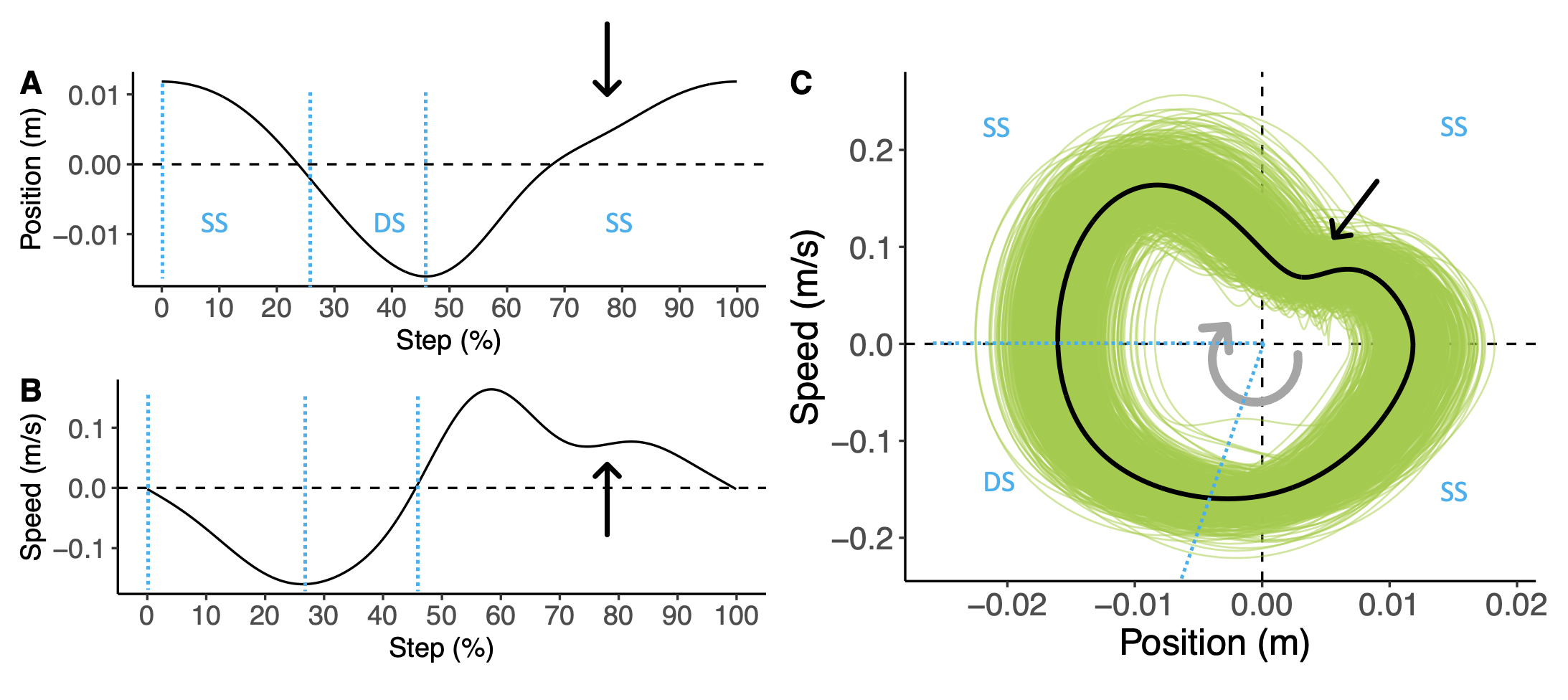
Figure 1: A: Attractor of the centred vertical position of the COM versus time, expressed in % of step time. B: Attractor of the vertical speed of the COM versus time, expressed in % of step time. C: Typical plot of COM vertical trajectory in phase space (solid green lines representing 508 gait cycles) during walking for a participant and of the corresponding attractor (solid black line). The straight arrows outline the deviation from genuine harmonic oscillator. The curved arrow is the arrow of time. Note that a closed loop corresponds to one step cycle, a complete gait cycle being composed of two step cycles. The blue dotted line separate the single stance (SS) and dual stance (DS) phases.

Table 2: Results of the fits of experimental distributions of the adiabatic invariants to model (6). Results are written under the form median [Q1$-$Q3]. The $p-$values of the one-sample t-tests are given in the last column.

$D$ (10-9 m2/s)	11.618 [6.024$-$37.712]	¡0.001
$\pi\ I_{0}$ (J.s/kg)	0.0123 [0.0061$-$0.0178]	¡0.001
$\Pi$ (%)	100 [98.6-100]

It appears that the fit is relevant since $\Pi>\,$97% for 20 participants out of 25. Hence, the model (6) fairly well agrees with the time evolution of the distribution of the adiabatic invariant. Fitted parameters are summarized in Table 2. The mean value of $I$ reads

$$\left\langle I\right\rangle=\int^{+\infty}_{0}\rho(I,t)dI=\frac{\Theta(t)}{{\rm erf}\left(\frac{I_{0}}{\sqrt{4Dt}}\right)}\ I_{0}\;,$$ (10)

and its behaviour versus time is displayed in Fig. 2. The mean value stays of order $I_{0}$ during the protocol: Less than 10 % of variation is observed. The values obtained are comparable to the mean value found by an independent analysis in Buisseret et al. (2022): $\pi\,I=$0.0143$\pm$0.0058 J.s/kg.

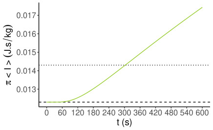
Figure 2: Plot of $\pi\,\left\langle I\right\rangle$ versus time (green line). The median value given in Table 2 is indicated (dashed line), as well as the average value found in Buisseret et al. (2022) (dotted line).

The ability of the model to fit the data can be appraised in Fig. 3, where a typical plot of the fitted distributions versus experimental observations is displayed for one participant. All participants show the same qualitative agreement between the model and the data.

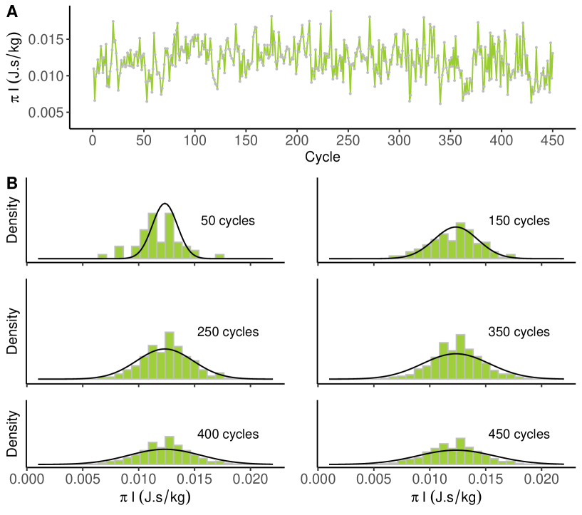
Figure 3: A: Adiabatic invariant versus time (gray points) for a given participant. Lines are added to guide the eyes, and time is expressed in cycle number. B: Typical plots showing the comparison between the theoretical distribution $\rho^{{\rm th}}(t_{i},I)$ (solid line) and the experimental one $\rho^{{\rm exp}}(t_{i},I)$ (histograms) after 50, 150, 250, 350, 400 and 450 cycles for the same participant as in A, with $\Pi=99.4$%. Fitted parameters are equal to $\pi\,I_{0}=0.0123$ J.s/kg and $D=1.05\,10^{-8}$ m²/s.

V Discussion

By studying the vertical motion of the healthy participant during walking, we have shown that the phenomenon of phase space diffusion can be observed through the distribution of adiabatic invariant values over time. To our knowledge, this is the first time that such an observation is made in human motion.

The time evolution of the distribution of the adiabatic invariant over time is compatible with the Fokker-Planck equation with constant diffusion coefficient for healthy young adults walking at spontaneous speed of progression. Thus, up to our experimental precision, we observe no drift and no deformation of the constant-$D$ distribution for high or low values of $I$. A change in the most likely value of $I$ can presumably be associated with a change in energy expenditure during walking. As argued in Buisseret et al. (2022), the value of the adiabatic invariant should be proportional to oxygen consumption during walking, and an increase in the former should be associated with an increase in the latter.

There are a number of immutable factors in the environment in which we live. One is gravity. The brain, instead of fighting against the effects caused by its presence (e.g. the emergence of a weight that counteracts movements) has developed strategies to make the most of it and optimize movements White et al. (2020). In other words, humans move more optimally in the presence than in the absence of a gravitational field. We can make a parallel with the existence of noise in physiological systems. These emerge at every level of the decision-action chain, from perception to motoneurons. Authors have proposed in the optimal movement variability framework, that the central nervous system could actually exploit the presence of noise and hence, act more optimally in the presence of certain levels of uncertainties. Following Goldberger et al. (2002); Stergiou et al. (2006); van Emmerik et al. (2016) we interpret the variability measured by the distribution not as an “imperfection” but rather as an indication of the adaptability of the participants to the motor task. A given value of the adiabatic invariant corresponds to a given area in phase space for the step cycle under consideration. Thus, the changes in $I$ indicate that the participants have access to a wide range of motor strategies, visualised as closed step cycles in phase space. The distribution becomes wider and wider over time: more and more different motor patterns are “explored”. In our approach, there is no drift: the most likely value of $I$, i.e. the attractor defined as the ideal trajectory in phase space that the participant is aiming for, does not change with time.

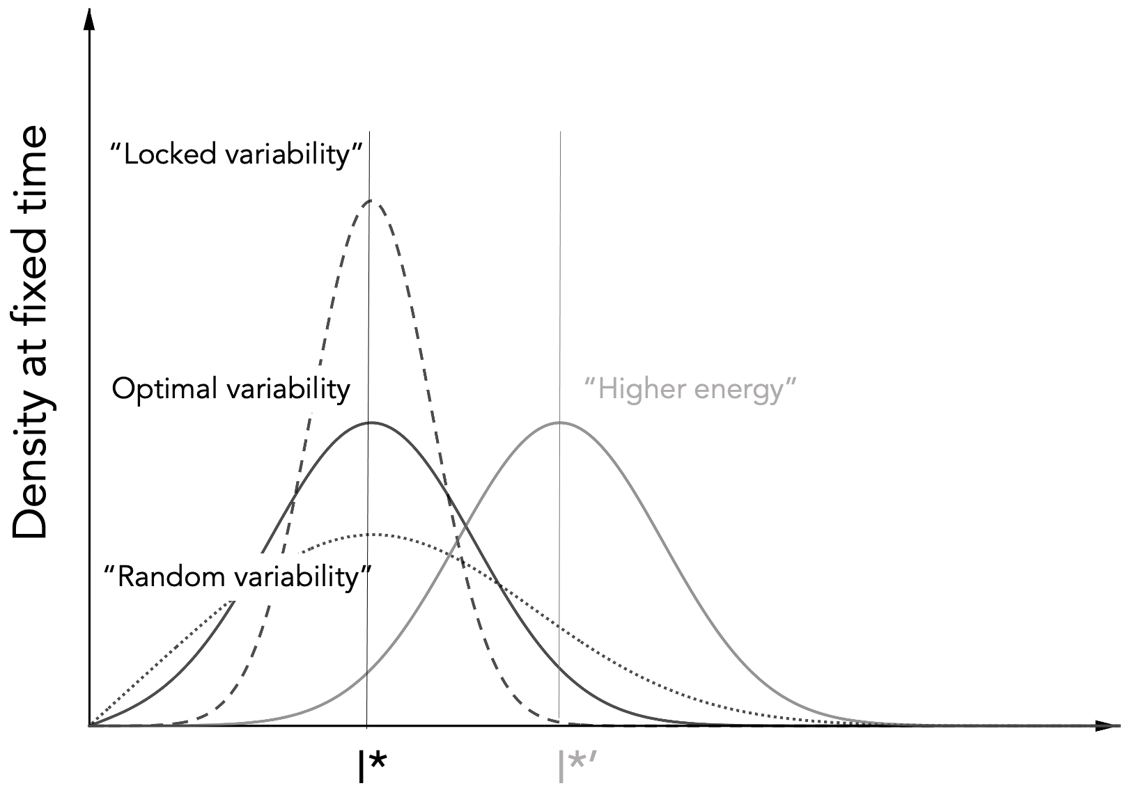
Figure 4: Schematic representation of several types of adiabatic invariant densities. We assume that the black solid line is the density of a young, healthy, individual. The “locked” (dashed line) and “random” (dotted line) curves correspond to, respectively, smaller and higher diffusion coefficients than the optimal one. The “higher energy” curve (gray solid line) has an optimal diffusion coefficient but a higher maximally probable $I^{*}$, denoted $I^{*}$’ on the horizontal axis.

We conjecture that the shape of the distribution $\rho(I,t)$ might be sensitive to the experimental condition and/or to each participant, as shown in Fig. 4. In particular, there should be an optimal value for the diffusion coefficient $D$ and for $I_{0}$ for a young, healthy individual. Too large a value for $D$ would reflect a lack of or altered motor control of the participant, leading to variability that tends to be random, as observed in stride interval variability of patients with neurodegenerative diseases Moon et al. (2016) for example. Too small a value for $D$ could be related to insufficient adaptability of the participant: the number of available patterns (i.e. different values of $I$) is not maximal. Such a case is observed, for example, in the electrocardiographic signal of patients with cardiovascular disease Goldberger et al. (2002) or in healthy children, whose walking patterns are more stereotyped than in adults Hausdorff et al. (1999). The diffusion coefficient then offers a novel way to quantify the general behaviour of internal models developed for a given task. Indeed, wide distribution (high D) are observed after time spent to experience or explore a task. On the other hand, narrow distributions (small D) may reflect a lack of generalisation of the motor strategies adopted. In motor control – and rehabilitation in particular – the concept of generalisation is tightly linked to the one of transfer Dizio and Lackner (1995); Criscimagna-Hemminger et al. (2003); Sarwary et al. (2015). When working toward recovering lost or impaired motor functions, the challenge is to find the best possible movements that may be transferred to as many functional tasks as possible. These movements may be interpreted as fundamental bricks of the action repertoire. An interesting question is why would a participant opt for a narrow distribution? One possible explanation for this is related to the way motor learning works. There are different learning mechanisms, the most powerful being error-based learning. In this one, one plans the best possible action by minimising a cost function that includes target reaching in the general sense and effort. An error signal is observed in case of discrepancy between observation and what has been predicted by forward models Shadmehr and Mussa-Ivaldi (1994); Thoroughman and Shadmehr (2000) which induces strategic changes, and encourage exploration. Another learning mechanisms, however, co-exists, with a slower dynamics: use-dependent-learning. When relying on this mechanism, one tends to repeat the same action if it led to success in the past, thereby discouraging exploration in task space. Adopting this strategy results from a compromise between cost and benefit: the target may be reached, but the control policy may be stuck in a local minima of the cost function.

We hope to apply the present formalism to participants with different ages or experimental conditions to investigate the effects of deviations from the optimal “healthy young adult state” on $\rho(I,t)$ in future work. More precisely, we hope to design appropriate experimental contexts that would manipulate $I$ and $D$ independently, then providing a better functional understanding of these indexes in motor control.

Acknowledgements

The authors thank G. Henry and F. Piccinin for data acquisition.

References

- Landau and Lifchitz (1988) Landau, L.; Lifchitz, E. Physique théorique Tome 1 : Mécanique; E. MIR: Moscow, 1988.
- Kolmogorov (1954) Kolmogorov, A.N. On conservation of conditionally periodic motions for a small change in Hamilton’s function. Dokl. Akad. Nauk SSSR 1954, 98, 527–530.
- Arnol’d (1963) Arnol’d, V.I. Proof of a theorem of A.N. Kolmogorov on the invariance of quadi-periodic motions under small perturbations of the hamiltonian. Russian Mathematical Surveys 1963, 18, 9–36.
- Möser (1962) Möser, J. On invariant curves of area-preserving mappings of an annulus. Nachr. Akad. Wiss. Göttingen, II 1962, pp. 1–20.
- Dumas (2014) Dumas, H. The KAM story: a friendly introduction to the content, history, and significance of classical Kolmogorov-Arnold-Moser theory; World Scientific: Hackensack, NJ, 2014.
- Nekhoroshev (1971) Nekhoroshev, N. Behavior of Hamiltonian systems close to integrable. Functional Analysis and Its Applications 1971, 5, 338–339.
- Nekhoroshev (1977) Nekhoroshev, N. An exponential estimate of the time of stability of nearly-integrable Hamiltonian systems. Uspekhi Matematicheskikh Nauk 1977, 32, 5–66.
- Henrard (1998) Henrard, J., The Adiabatic Invariant in Classical Mechanics. In Dessy Proceedings 1998-03; Dessy, 1998; pp. 60–73.
- Jose and Saletan (1998) Jose, J.; Saletan, E. Classical dynamics: a contemporary approach; Cambridge Univ. Press: Cambridge, 1998.
- Khas’minskiĭ (1966) Khas’minskiĭ, R.Z. On Stochastic Processes Defined by Differential Equations with a Small Parameter. Theory of Probability and Its Applications 1966, 11, 211–228.
- Cogburn and Ellison (1992) Cogburn, R.; Ellison, J.A. A stochastic theory of adiabatic invariance. Communications in Mathematical Physics 1992, 149, 97–126.
- Bazzani et al. (1994) Bazzani, A.; Siboni, S.; Turchetti, G.; Vaienti, S. A model of modulated diffusion. I. Analytical results. Journal of Statistical Physics 1994, 76, 929–967.
- Bazzani et al. (1995) Bazzani, A.; Siboni, S.; Turchetti, G. Diffusion in stochastically and periodically modulated Hamiltonian systems. AIP Conference Proceedings 1995, 344, 68–77, [https://aip.scitation.org/doi/pdf/10.1063/1.48970].
- Bazzani and Beccaceci (1998) Bazzani, A.; Beccaceci, L. Diffusion in Hamiltonian systems driven by harmonic noise. Journal of Physics A: Mathematical and General 1998, 31, 5843–5854.
- Kominis et al. (2010) Kominis, Y.; Ram, A.K.; Hizanidis, K. Kinetic Theory for Distribution Functions of Wave-Particle Interactions in Plasmas. Phys. Rev. Lett. 2010, 104, 235001.
- Degond et al. (2020) Degond, P.; Herda, M.; Mirrahimi, S. A Fokker-Planck approach to the study of robustness in gene expression. Mathematical Biosciences and Engineering 2020, 17, 6459–6486.
- Hausdorff et al. (1995) Hausdorff, J.; Peng, C.; Ladin, Z.; Wei, J.; Goldberger, A. Is walking a random walk? Evidence for long-range correlations in stride interval of human gait. Journal of Applied Physiology 1995, 78, 349–358.
- Hausdorff et al. (1997) Hausdorff, J.; Mitchell, S.; Firtion, R.; Peng, C.; Cudkowicz, M.; Wei, J.; Goldberger, A. Altered fractal dynamics of gait: reduced stride-interval correlations with aging and Huntington’s disease. Journal of Applied Physiology 1997, 82, 262–269.
- Stergiou (2016) Stergiou, N.A. Nonlinear Analysis for Human Movement Variability; Vol. 7, CRC Press, 2016.
- Ravi et al. (2020) Ravi, D.K.; Marmelat, V.; Taylor, W.R.; Newell, K.M.; Stergiou, N.; Singh, N.B. Assessing the Temporal Organization of Walking Variability: A Systematic Review and Consensus Guidelines on Detrended Fluctuation Analysis. Frontiers in Physiology 2020, 11.
- Risken and Haken (1989) Risken, H.; Haken, H. The Fokker-Planck Equation: Methods of Solution and Applications Second Edition; Springer, 1989.
- Fa (2005) Fa, K.S. Exact solution of the Fokker-Planck equation for a broad class of diffusion coefficients. Phys. Rev. E 2005, 72, 020101.
- Lin and Ho (2012) Lin, W.T.; Ho, C.L. Similarity solutions of the Fokker–Planck equation with time-dependent coefficients. Annals of Physics 2012, 327, 386–397.
- Cavagna et al. (1976) Cavagna, G.; Thys, H.; Zamboni, A. The sources of external work in level walking and running. J Physiol. 1976, 262, 639–657.
- Cavagna and Legramandi (2020) Cavagna, G.A.; Legramandi, M.A. The phase shift between potential and kinetic energy in human walking. Journal of Experimental Biology 2020, 223, [https://journals.biologists.com/jeb/article-pdf/223/21/jeb232645/1982510/jeb232645.pdf].
- Whittington and Thelen (2008) Whittington, B.R.; Thelen, D.G. A Simple Mass-Spring Model With Roller Feet Can Induce the Ground Reactions Observed in Human Walking. Journal of Biomechanical Engineering 2008, 131, [https://asmedigitalcollection.asme.org/biomechanical/article-pdf/131/1/011013/5521702/011013_1.pdf].
- Brizard (2013) Brizard, A.J. Jacobi zeta function and action-angle coordinates for the pendulum. Communications in Nonlinear Science and Numerical Simulation 2013, 18, 511–518.
- Buisseret et al. (2022) Buisseret, F.; Dehouck, V.; Boulanger, N.; Henry, G.; Piccinin, F.; White, O.; Dierick, F. Adiabatic Invariant of Center-of-Mass Motion during Walking as a Dynamical Stability Constraint on Stride Interval Variability and Predictability. Biology 2022, 11.
- Sturges (1926) Sturges, H.A. The Choice of a Class Interval. Journal of the American Statistical Association 1926, 21, 65–66, [https://doi.org/10.1080/01621459.1926.10502161].
- Broscheid et al. (2018) Broscheid, K.C.; Dettmers, C.; Vieten, M. Is the Limit-Cycle-Attractor an (almost) invariable characteristic in human walking? Gait and Posture 2018, 63, 242–247.
- Raffalt et al. (2020) Raffalt, P.; Kent, J.; Wurdeman, S.; N., S. To walk or to run - a question of movement attractor stability. J Exp Biol. 2020, 223, 1.
- Whittington and Thelen (2009) Whittington, B.; Thelen, D. A simple mass-spring model with roller feet can induce the ground reactions observed in human walking. J Biomech Eng. 2009, 131, 011013.
- Adamczyk and Kuo (2009) Adamczyk, P.G.; Kuo, A.D. Redirection of center-of-mass velocity during the step-to-step transition of human walking. Journal of Experimental Biology 2009, 212, 2668–2678, [https://journals.biologists.com/jeb/article-pdf/212/16/2668/1558857/2668.pdf].
- White et al. (2020) White, O.; Gaveau, .J.; Bringoux, L.; Crevecoeur, F. The gravitational imprint on sensorimotor planning and control. J. Neurophysiol. 2020, 124, 4–19.
- Goldberger et al. (2002) Goldberger, A.L.; Amaral, L.A.N.; Hausdorff, J.M.; Ivanov, P.C.; Peng, C.K.; Stanley, H.E. Fractal dynamics in physiology: Alterations with disease and aging. Proceedings of the National Academy of Sciences 2002, 99, 2466–2472, [https://www.pnas.org/doi/pdf/10.1073/pnas.012579499].
- Stergiou et al. (2006) Stergiou, N.; Harbourne, R.; Cavanaugh, J. Optimal movement variability: a new theoretical perspective for neurologic physical therapy. J Neurol Phys Ther. 2006, 30, 120–9.
- van Emmerik et al. (2016) van Emmerik, R.E.; Ducharme, S.W.; Amado, A.C.; Hamill, J. Comparing dynamical systems concepts and techniques for biomechanical analysis. Journal of Sport and Health Science 2016, 5, 3–13.
- Moon et al. (2016) Moon, Y.; Sung, J.; An, R.; Hernandez, M.E.; Sosnoff, J.J. Gait variability in people with neurological disorders: A systematic review and meta-analysis. Human Movement Science 2016, 47, 197–208.
- Goldberger et al. (2002) Goldberger, A.L.; Amaral, L.A.N.; Hausdorff, J.M.; Ivanov, P.C.; Peng, C.K.; Stanley, H.E. Fractal dynamics in physiology: Alterations with disease and aging. Proceedings of the National Academy of Sciences 2002, 99, 2466–2472, [https://www.pnas.org/doi/pdf/10.1073/pnas.012579499].
- Hausdorff et al. (1999) Hausdorff, J.; Zemany, L.; Peng, C.K.; Goldberger, A. Maturation of gait dynamics: stride-to-stride variability and its temporal organization in children. Journal of applied physiology 1999, 86, 1040–1047.
- Dizio and Lackner (1995) Dizio, P.; Lackner, J.R. Motor adaptation to Coriolis force perturbations of reaching movements: endpoint but not trajectory adaptation transfers to the nonexposed arm. Journal of Neurophysiology 1995, 74, 1787–1792, [https://doi.org/10.1152/jn.1995.74.4.1787].
- Criscimagna-Hemminger et al. (2003) Criscimagna-Hemminger, S.E.; Donchin, O.; Gazzaniga, M.S.; Shadmehr, R. Learned Dynamics of Reaching Movements Generalize From Dominant to Nondominant Arm. Journal of Neurophysiology 2003, 89, 168–176, [https://doi.org/10.1152/jn.00622.2002].
- Sarwary et al. (2015) Sarwary, A.M.E.; Stegeman, D.F.; Selen, L.P.J.; Medendorp, W.P. Generalization and transfer of contextual cues in motor learning. Journal of Neurophysiology 2015, 114, 1565–1576, [https://doi.org/10.1152/jn.00217.2015].
- Shadmehr and Mussa-Ivaldi (1994) Shadmehr, R.; Mussa-Ivaldi, F. Adaptive representation of dynamics during learning of a motor task. J Neurosci. 1994, 14, 3208–3224.
- Thoroughman and Shadmehr (2000) Thoroughman, K.A.; Shadmehr, R. Learning of action through adaptive combination of motor primitives. Nature 2000, 407, 742–747.