This paper has been accepted for publication in IEEE Transactions on Robotics.

This is the author’s version of an article that has, or will be, published in this journal or conference. Changes were, or will be, made to this version by the publisher prior to publication.

DOI:	10.1109/TRO.2022.3229842
IEEE Xplore:	https://ieeexplore.ieee.org/document/10026622

Please cite this paper as:

T. Hitchcox and J. R. Forbes, “Improving Self-Consistency in Underwater Mapping Through Laser-Based Loop Closure,” IEEE Transactions on Robotics, vol. 39, no. 3, pp. 1873-1892, 2023.

©2023  IEEE. Personal use of this material is permitted. Permission from IEEE must be obtained for all other uses, in any current or future media, including reprinting/republishing this material for advertising or promotional purposes, creating new collective works, for resale or redistribution to servers or lists, or reuse of any copyrighted component of this work in other works.

Improving Self-Consistency in Underwater Mapping Through Laser-Based Loop Closure (Extended)

Abstract

Accurate, self-consistent bathymetric maps are needed to monitor changes in subsea environments and infrastructure. These maps are increasingly collected by underwater vehicles, and mapping requires an accurate vehicle navigation solution. Commercial off-the-shelf (COTS) navigation solutions for underwater vehicles often rely on external acoustic sensors for localization, however survey-grade acoustic sensors are expensive to deploy and limit the range of the vehicle. Techniques from the field of simultaneous localization and mapping, particularly loop closures, can improve the quality of the navigation solution over dead-reckoning, but are difficult to integrate into COTS navigation systems. This work presents a method to improve the self-consistency of bathymetric maps by smoothly integrating loop-closure measurements into the state estimate produced by a commercial subsea navigation system. Integration is done using a white-noise-on-acceleration motion prior, without access to raw sensor measurements or proprietary models. Improvements in map self-consistency are shown for both simulated and experimental datasets, including a 3D scan of an underwater shipwreck in Wiarton, Ontario, Canada.

I Introduction

Accurate, self-consistent bathymetric maps are critical for assessing the health of subsea environments and infrastructure. Increasingly, these maps are collected by autonomous underwater vehicles (AUVs) using a variety of on-board sensors, including cameras [1, 2, 3], sonar [4, 5, 6], and laser scanners [7, 8]. Since the map is constructed using the estimated AUV trajectory, long-term navigation accuracy is a prerequisite for building accurate maps.

The standard navigation solution for commercial AUVs is a commercial off-the-shelf (COTS) inertial navigation system (INS), with acoustic aiding from a Doppler velocity log (DVL). The dead-reckoned precision of these systems is measured by drift rate as a percent of distance traveled, with high-quality DVL-INS systems achieving a drift rate of as low as $0.01\text{\,}\mathrm{\char 37\relax}$. However, without localizing measurements the precision of the state estimate will deteriorate without bound, impacting long-term accuracy.

Since GPS signals attenuate rapidly in water, AUV localization is primarily done using acoustics [9]. For example, long baseline (LBL) arrays are acoustic beacons installed on the seafloor that trilaterate the position of an AUV, much like an “acoustic GPS.” Short baseline (SBL) and ultrashort baseline (USBL) systems are affixed to a surface vessel, and measure the acoustic range and bearing of an underwater vehicle. These sensors are frequently deployed in a commercial setting, and have been used to aid AUV navigation in the literature, for example [10].

Figure 1: A point cloud map of an actual shipwreck collected in Wiarton, Ontario, Canada, where colour represents relative depth. The top map is generated using the state estimate produced by a commercial off-the-shelf (COTS) Doppler velocity log-aided inertial measurement system (DVL-INS). The bottom map is generated using the proposed method, which conditions the DVL-INS estimate on loop-closure measurements without access to the raw DVL-INS sensor measurements. Note the improvement in map self-consistency when loop-closure measurements are included.

Acoustic positioning systems enable accurate and precise AUV trajectory estimates, however they are expensive to deploy and limit the mission domain of the vehicle. For example, LBL systems are time-consuming to install and calibrate, while SBL and USBL systems require the presence of a large surface vessel. In addition, acoustic positioning systems produce measurements with limited precision, which may lead to small irregularities in a composite map built from several overlapping measurements of the same area. This in turn may make it difficult to assess relative distances and deformation, or other measurements critical to subsea safety.

I-A Motivation

Loop closures play a central role in many simultaneous localization and mapping (SLAM) algorithms, whereby a vehicle returns to and is able to recognize a previously explored region of the map. Loop-closure measurements effectively “reset” any navigation drift accumulated throughout the loop [11], resulting in navigation solutions that are both more accurate and more precise than dead-reckoning, without the need for external localizing measurements. Multiple loop closures over time lead to bounded navigation drift and a more self-consistent map estimate, whereby the resulting map is free of irregularities and “double vision” effects produced by poorly aligned measurements, an example of which is shown in Figure 1. This is not to be confused with the term consistent, which in the context of state estimation describes a solution for which the covariance bounds accurately reflect the error in the mean state estimate [12, Sec. 5.4.2].

Previous applications of SLAM for underwater mapping leverage loop-closure measurements to improve map self-consistency. However, these applications have largely been implemented on research platforms with access to raw sensor measurements and full knowledge of the state estimation algorithm. In contrast, commercial “strapdown” DVL-INS systems for subsea navigation produce a state estimate, and due to their proprietary nature rarely provide access to

1. raw sensor measurements, including interoceptive measurements $\mbf{u}_{k}$, such as from an IMU, and exteroceptive measurements $\mbf{y}_{\ell}$, such as from a DVL;

2. a process model of the form

   $$\tilde{\mbf{x}}_{k}=\mbf{f}_{k-1}(\mbf{x}_{k-1},\mbf{u}_{k-1}),$$ (1)

   which describes how the vehicle moves throughout time;

3. sensor models of the form

   $$\tilde{\mbf{y}}_{\ell}=\mbf{g}_{\ell}(\mbf{x}_{\ell},\mbf{v}_{\ell}),$$ (2)

   which allow for predicted measurements; and

4. sensor noise and bias specifications, for example

   $$\mbf{u}(t)= \ \bar{\mbf{u}}(t)+\bm{\beta}(t)+\mbf{w}(t),$$ (3a)

   $$\dot{\bm{\beta}}(t)\sim \ \mathcal{N}(\mbf{0},\bm{\mathcal{Q}}_{\dot{\beta}}\delta(t-t^{\prime})),$$ (3b)

   $$\mbf{w}(t)\sim \ \mathcal{N}(\mbf{0},\bm{\mathcal{Q}}_{w}\delta(t-t^{\prime})),$$ (3c)

   where $\mbf{u}$ is known to be corrupted by time-varying random walk bias $\bm{\beta}$ and Gaussian white noise $\mbf{w}$, characterized by power spectral densities $\bm{\mathcal{Q}}_{\dot{\beta}}$ and $\bm{\mathcal{Q}}_{w}$, respectively.

Commercial DVL-INS systems, for example the Sonardyne SPRINT-Nav 500 [13], are effectively “black boxes,” and their lack of transparency makes it difficult to incorporate loop-closure measurements using conventional state estimation tools [14, 15], as illustrated by the factor graph [16] in Figure 2.

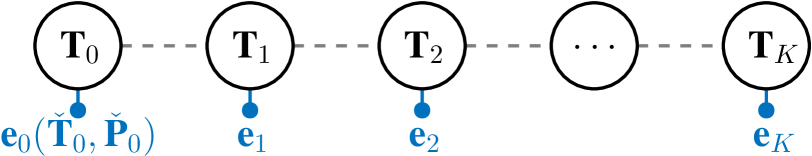
Figure 2: A factor graph depicting the output from a commercial DVL-INS. Only the estimated trajectory $\check{\mbf{T}}_{0:K}$ and incomplete marginal covariance matrices $\check{\mbf{P}}_{0:K}$ are available, leading to the formation of prior factors $\mbf{e}_{0:K}$. Without factors linking adjacent nodes, loop-closure corrections cannot propagate throughout the graph, and the trajectory cannot be updated.

I-B Prior Work

The field of simultaneous localization and mapping has found ample application in the domain of subsea robotics. For example, [4] produced a self-consistent bathymetric map of two hydrothermal vents by aligning point cloud submaps generated using multibeam sonar. A distributed particle mapping algorithm was described in [5], where particle weighting was determined based on the innovation between multibeam sonar measurements and the existing map. However, the map resolution was limited by the selection of a grid cell size. This limitation was later addressed in [17], which adopted Gaussian processes as a map representation. The submap alignment approach was followed by [18], which demonstrated improvements in submap simplification and point cloud alignment in a harbour scanning application. Harbour scanning and surveillance was also the subject of [19], which used a feature-based approach to align point clouds collected from imaging sonar. Recent research has focused on more structured environments, for example ship hull inspection [1, 20, 6, 21, 22] and subsea infrastructure [7].

These studies generally had access to the information enumerated in Section I-A, and as a result were able to incorporate loop-closure measurements using conventional state estimation techniques. For example, [4] applied loop-closure measurements within an extended Kalman filtering framework, and enjoyed access to raw navigation sensor measurements as well as a vehicle process model. Individual particles in [5] and [17] were propagated forward using DVL measurements and a constant-velocity motion model. The research platform used in the related ship hull inspection studies [1, 20, 6, 21, 22] produced raw DVL, IMU, and depth sensor measurements, while the platform in [3] had access to a variety of raw sensor measurements including stereo vision and profiling sonar. These applications used conventional pose-graph SLAM to incorporate loop-closure measurements produced by various exteroceptive sensors.

I-C Contribution

This work describes a novel approach to underwater mapping using a high-resolution laser line scanner and the output of a commercial DVL-INS navigation system. First, this work develops a robust laser-based front-end algorithm to produce high-precision loop-closure measurements by aligning point cloud scans collected in challenging underwater environments. Next, this work shows how to cleanly fuse loop-closure measurements into the output of a survey-grade COTS DVL-INS system via factor graph optimization. As these commercial systems are typically “black boxes” which only provide a navigation estimate, the proposed approach shows how to systematically incorporate loop-closure measurements without access to raw sensor measurements or other information typically required in state estimation tasks. In contrast to previous approaches, the proposed methodology also enforces a smoothness requirement on the posterior trajectory estimate. This eliminates discontinuities often encountered in dead-reckoned trajectory estimates, and is critical for accurate feature detection in laser submaps. In summary, the proposed methodology describes a robust and comprehensive system for high-precision, self-consistent underwater mapping using COTS navigation systems. Improvements to both map self-consistency and the relative accuracy of the trajectory estimate are rigorously evaluated in simulation and on an actual underwater mapping dataset.

I-D Paper Organization

This paper is organized as follows. Section II contains preliminary information on conventions used, state estimation on matrix Lie groups, and batch state estimation. Section III introduces the methodology, including the formulation of loop-closure measurements from laser scan data and the construction of the batch optimization problem. Section IV contains results on simulated and field datasets. The paper concludes in Section V with a review of the findings and opportunities for future work.

II Preliminaries

II-A Reference Frames and Navigation Conventions

This section discusses the conventions for attitude and displacement used in this paper. A three-dimensional dextral reference frame ${\mathcal{F}_{a}}$ is composed of three orthonormal physical basis vectors. The position of physical point $\color[rgb]{0,0,0}{z}\color[rgb]{0,0,0}$ relative to point $\color[rgb]{0,0,0}{w}\color[rgb]{0,0,0}$, denoted by ${\underrightarrow{{r}}}^{\color[rgb]{0,0,0}{zw}\color[rgb]{0,0,0}}$, is resolved in reference frame ${\mathcal{F}_{a}}$ as ${\mbf{r}_{a}^{\color[rgb]{0,0,0}{zw}\color[rgb]{0,0,0}}}$ and in reference frame ${\mathcal{F}_{b}}$ as $\mbf{r}_{b}^{zw}$. These these quantities are related via ${\mbf{r}^{zw}_{a}=\mbf{C}_{ab}\mbf{r}^{zw}_{b}}$, where $\mbf{C}_{\color[rgb]{0,0,0}{ab}\color[rgb]{0,0,0}}$ is a direction cosine matrix, ${\mbf{C}\in SO(3)=\{\mbf{C}\in\mathbb{R}^{3\times 3}\,|\,\mbf{C}\mbf{C}^{\mathsf{T}}=\mbf{1},\det\mbf{C}=+1\}}$ [23]. Time-varying quantities are indicated by the subscript $(\cdot)_{k}$, for example $\mbf{r}^{z_{k}w}_{a}$ describes the position of moving point $z$ at time $t_{k}$. In this work, point $z$ is affixed to the vehicle, while $w$ denotes the stationary point in the world. Body frame ${\mathcal{F}_{b}}$ rotates with the vehicle, while local geodetic frame ${\mathcal{F}_{a}}$ remains stationary. Both ${\mathcal{F}_{b}}$ and ${\mathcal{F}_{a}}$ are north-east-down (NED), in agreement with maritime convention.

II-B Matrix Lie Groups

The attitude and position of a vehicle at time $t_{k}$, collectively referred to as the vehicle’s “pose,” may be conveniently represented in 3D space as an element of matrix Lie group $SE(3)$ [23, Sec. 7.1.1],

$$\mbf{T}^{z_{\color[rgb]{0,0,0}{k}\color[rgb]{0,0,0}}w}_{ab_{\color[rgb]{0,0,0}{k}\color[rgb]{0,0,0}}}=\begin{bmatrix}\mbf{C}_{ab_{\color[rgb]{0,0,0}{k}\color[rgb]{0,0,0}}}&\mbf{r}^{z_{\color[rgb]{0,0,0}{k}\color[rgb]{0,0,0}}w}_{a}\\ \mbf{0}&1\end{bmatrix}\in SE(3),$$ (4)

with ${SE(3)=\{\mbf{T}\in\mathbb{R}^{4\times 4}\,|\,\mbf{C}\in SO(3),\mbf{r}\in\mathbb{R}^{3}\}}$. Associated with every matrix Lie group is a matrix Lie algebra, defined as the tangent space at the group identify [24]. For $SE(3)$, this is $\mathfrak{se}(3)\triangleq T{1}SE(3)$. For estimation problems involving matrix Lie groups, the matrix Lie algebra is a convenient space to represent perturbations and uncertainty. An element of $\mathfrak{se}(3)$ is given by [25, Sec. 2.3]

$$\bm{\xi}^{\wedge}=\begin{bmatrix}\bm{\phi}\\ \bm{\rho}\end{bmatrix}^{\wedge}=\begin{bmatrix}0&-\phi_{3}&\phi_{2}&\rho_{1}\\ \phi_{3}&0&-\phi_{1}&\rho_{2}\\ -\phi_{2}&\phi_{1}&0&\rho_{3}\\ 0&0&0&0\end{bmatrix}\in\mathfrak{se}(3),$$ (5)

where ${(\cdot)^{\wedge}:\mathbb{R}^{6}\to\mathfrak{se}(3)}$ is an isometric operator. The inverse of this operator is ${(\cdot)^{\vee}:\mathfrak{se}(3)\to\mathbb{R}^{6}}$, such that ${(\bm{\xi}^{\wedge})^{\vee}=\bm{\xi}}$. A Lie group and Lie algebra are related through the exponential map, which for matrix Lie groups is the matrix exponential,

$$\mbf{T}=\exp(\bm{\xi}^{\wedge}).\vspace{-1pt}$$ (6)

The matrix logarithm is used to return to the Lie algebra via

$$\bm{\xi}^{\wedge}=\log(\mbf{T}).\vspace{-1pt}$$ (7)

Elements of the matrix Lie algebra are combined according to the Baker-Campbell-Hausdorff (BCH) equation,

$$\bm{\gamma}^{\wedge}=\log\left(\exp(\bm{\xi}^{\wedge})\exp(\bm{\eta}^{\wedge})\right).\vspace{-1pt}$$ (8)

An approximation to the BCH equation for ${\bm{\xi}\gg\bm{\eta}}$ is

$$\bm{\gamma}^{\wedge}\approx(\bm{\xi}+\mbf{J}^{\textrm{r}}(\bm{\xi})^{-1}\bm{\eta})^{\wedge},\vspace{-1pt}$$ (9)

where $\mbf{J}^{\textrm{r}}$ is the right Jacobian of $SE(3)$ [23, Sec. 7.1.5].

Errors on matrix Lie groups are defined multiplicatively. This work uses the left-invariant error definition,

$$\delta\mbf{T}=\mbf{T}^{-1}\tilde{\mbf{T}},\vspace{-3pt}$$ (10)

where $\mbf{T}$ is the current state estimate and $\tilde{\mbf{T}}$ is a state estimate generated from sensor measurements or prior information. The corresponding perturbation scheme is

$$\mbf{T}=\bar{\mbf{T}}\exp(-\delta\bm{\xi}^{\wedge}),\vspace{-1pt}$$ (11)

with perturbation ${\delta\bm{\xi}\sim\mathcal{N}(\mbf{0},\mbf{P})}$, ${\mbf{P}=\mathrm{E}[\delta\bm{\xi}\,\delta\bm{\xi}^{\mathsf{T}}]\in\mathbb{R}^{6\times 6}}$. Note the negative sign in (11) ensures consistency with the left-invariant error definition (10). The state estimate is therefore defined by mean estimate $\bar{\mbf{T}}$ and covariance $\mbf{P}$.

This work makes frequent use of the adjoint matrix $\operatorname{\mbf{Ad}}(\mbf{T})$, which maps perturbations about the group identity to other group elements [24]. Formally,

$$\operatorname{\mbf{Ad}}(\mbf{T})\delta\bm{\xi}\triangleq\left(\mbf{T}\delta\bm{\xi}^{\wedge}\mbf{T}^{-1}\right)^{\vee}.\vspace{-3pt}$$ (12)

For $SE(3)$, the adjoint matrix is [25]

$$\operatorname{\mbf{Ad}}(\mbf{T})=\begin{bmatrix}\mbf{C}&\mbf{0}\\ \mbf{r}^{\times}\mbf{C}&\mbf{C}\end{bmatrix},$$ (13)

where $(\cdot)^{\times}$ is the skew-symmetric operator [23, Sec. 7.1.2]. The adjoint matrix is represented in the matrix Lie algebra as

$$\left(\operatorname{\mbf{ad}}(\bm{\xi}^{\wedge}_{1})\bm{\xi}_{2}\right)^{\wedge}\triangleq\left[\bm{\xi}^{\wedge}_{1},\bm{\xi}^{\wedge}_{2}\right]=\bm{\xi}^{\wedge}_{1}\bm{\xi}^{\wedge}_{2}-\bm{\xi}^{\wedge}_{2}\bm{\xi}^{\wedge}_{1},$$ (14)

where $\left[\cdot,\cdot\right]$ is the Lie bracket [26, Sec. 10.2.6]. For $\mathfrak{se}(3)$,

$$\operatorname{\mbf{ad}}(\bm{\xi}^{\wedge})=\begin{bmatrix}\bm{\phi}^{\times}&\mbf{0}\\ \bm{\rho}^{\times}&\bm{\phi}^{\times}\end{bmatrix}.$$ (15)

II-C Gaussian Processes

A continuous-time Gaussian process (GP) may be viewed as a distribution over functions,

$$\mbf{f}(t)\sim\mathcal{GP}\left(\bm{\mu}(t),\bm{\Sigma}(t,t^{\prime})\right),$$ (16)

where $\bm{\mu}(t)$ is the mean function, and $\bm{\Sigma}(t,t^{\prime})$ is the covariance function [27, Sec. 2.2][23, Sec. 2.3]. For any finite collection of time steps $t_{0:K}$, $\mbf{f}(t_{0:K})$ follows a joint Gaussian distribution. The covariance function determines how individual function samples $\mbf{f}_{i}(t)$ covary over time. For example, a GP for which the covariance over time is large will be smoother than a GP for which the covariance over time is small. This work uses the zero-mean white noise GP, given by [23, Sec. 2.3]

$$\mbf{w}(t)\sim\mathcal{GP}(\mbf{0},\bm{\mathcal{Q}}\delta(t-t^{\prime})),$$ (17)

where $\bm{\mathcal{Q}}$ is a power spectral density matrix and $\delta(\cdot)$ is the Dirac delta function.

II-D The White-Noise-On-Acceleration Motion Prior

The white-noise-on-acceleration (WNOA) motion prior may be summarized by the following set of stochastic differential equations [28],

$$\dot{\mbf{T}}(t)= \ \mbf{T}(t)\bm{\varpi}_{b}(t)^{\wedge},$$ (18a)

$$\dot{\bm{\varpi}}_{b}(t)\sim \ \mathcal{GP}(\mbf{0},\bm{\mathcal{Q}}\delta(t-t^{\prime})).$$ (18b)

Equation 18a describes the continuous-time state kinematics for $SE(3)$, with ${\bm{\varpi}_{b}}$ the generalized velocity, such that ${T\bm{\varpi}^{\wedge}_{b}\in\mathfrak{se}(3)}$, with $T$ a time increment. The subscript $(\cdot)_{b}$ has been included to emphasize that $\bm{\varpi}$ is a body-frame quantity. The time rate of change of $\bm{\varpi}$ is distributed according to the zero-mean white noise Gaussian process in (18b), with power spectral density $\bm{\mathcal{Q}}$. Note that $\bm{\mathcal{Q}}$ is a hyperparameter that needs to be tuned. This motion prior helps to enforce smoothness is the posterior state estimate, as ${\mathrm{E}[\dot{\bm{\varpi}}]=\mbf{0}}$. In discrete time, this implies ${\mathrm{E}[\bm{\varpi}_{k}]=\bm{\varpi}_{k-1}}$. The white noise assumption also preserves sparsity in the upcoming batch problem [29].

The WNOA assumption is reasonable in the context of subsea navigation, as AUV kinematics evolve slowly over time. With the inclusion of $\bm{\varpi}$, the augmented navigation state becomes the ordered pair

$$\mbf{X}=\left(\mbf{T},\bm{\varpi}\right)\in SE(3)\times\mathbb{R}^{6}.$$ (19)

II-E Batch State Estimation

Given a set of exteroceptive measurements ${\{\mbf{y}_{\ell}\}^{L}_{\ell=1}}$, interoceptive measurements ${\{\mbf{u}_{k}\}^{K-1}_{k=0}}$, and prior estimate ${\mbf{Y}_{0}\!=\!\bar{\mbf{Y}}_{0}\exp(-\delta\bm{\eta}_{0}^{\wedge})}$, ${\mbf{S}_{0}\!=\!\mathrm{E}[\delta\bm{\eta}_{0}\,\delta\bm{\eta}_{0}^{\mathsf{T}}]}$, the standard approach to batch estimation is to produce a maximum a posteriori (MAP) solution, given by

$$\hat{\mbf{X}}=\operatorname*{arg\,max}_{\mbf{X}}\,p\!\left(\mbf{X}\,|\,\mbf{y}_{1:L},\mbf{u}_{0:K-1},\mbf{Y}_{0}\right).$$ (20)

Under the Markov assumption, the joint probability in (20) may be factored as

$$\hat{\mbf{X}}=\operatorname*{arg\,max}_{\mbf{X}}\prod^{L}_{\ell=1}p\left(\mbf{y}_{\ell}\hskip 0.50003pt\big{|}\hskip 0.50003pt\mbf{X}_{\ell}\right)\prod^{K}_{k=1}p\left(\mbf{X}_{k}\hskip 0.50003pt\big{|}\hskip 0.50003pt\mbf{X}_{k-1},\mbf{u}_{k-1}\right)p\left(\mbf{X}_{0}\hskip 0.50003pt\big{|}\hskip 0.50003pt\mbf{Y}_{0}\right).$$ (21)

Taking the negative log likelihood of (21) results in a nonlinear least-squares problem of the form

$$\hat{\mbf{X}}=\operatorname*{arg\,min}_{\mbf{X}}J(\mbf{X}),$$ (22)

where the objective function $J(\mbf{X})$ is given by

$$J(\mbf{X})= \ \frac{1}{2}\sum^{L}_{\ell=1}\left\|\mbf{e}_{\ell}(\bar{\mbf{y}}_{\ell},\mbf{g}_{\ell}(\bar{\mbf{X}}_{\ell},\mbf{0}))\right\|^{2}_{\mbf{R}^{-1}_{\ell}}+\frac{1}{2}\left\|\mbf{e}_{0}(\bar{\mbf{Y}}_{0},\bar{\mbf{X}}_{0})\right\|^{2}_{\mbf{S}^{-1}_{0}}$$

$$\ +\frac{1}{2}\sum^{K}_{k=1}\left\|\mbf{e}_{k}(\mbf{f}_{k-1}(\bar{\mbf{X}}_{k-1},\bar{\mbf{u}}_{k-1}),\bar{\mbf{X}}_{k})\right\|^{2}_{\mbf{Q}^{-1}_{k}}.$$ (23)

In (23), $\mbf{e}_{k}$, $\mbf{e}_{\ell}$, and $\mbf{e}_{0}$ are the interoceptive, exteroceptive, and prior errors, respectively, while $\mbf{f}_{k-1}$ and $\mbf{g}_{\ell}$ represent the nonlinear process and measurement models, respectively. The notation ${\left\|\mbf{e}\right\|^{2}_{\bm{\Sigma}^{-1}}=\mbf{e}^{\mathsf{T}}\bm{\Sigma}^{-1}\mbf{e}}$ denotes the squared Mahalanobis distance, and $\mbf{Q}_{k}$ and $\mbf{R}_{\ell}$ represent the discrete-time covariance on the interoceptive and exteroceptive errors, respectively. To minimize (22), (23) is repeatedly linearized about the current state estimate $\bar{\mbf{X}}$, and the local minimizing solution found using, for example, Gauss-Newton or Levenberg-Marquardt.

III Methodology

This section describes the primary contributions of this paper, namely the formulation of laser-based loop-closure measurements and the smooth incorporation of these measurements into a COTS DVL-INS trajectory estimate. An overview of the upcoming methodology is shown in Figure 3.

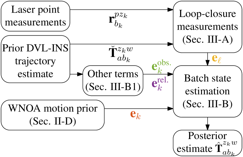
Figure 3: A visual overview of Section III. Note the colour of the error terms is consistent with the factor graph of Figure 6.

III-A Loop Closures from Subsea Point Cloud Scans

To correct for drift in the DVL-INS trajectory estimate, loop-closure measurements are obtained by aligning sections of the point cloud scan collected using a Voyis Insight Pro underwater laser scanner. The raw laser profiles are first filtered and registered to the trajectory estimate to produce a 3D point cloud. Loop-closure opportunities are identified at path crossings, and alignment is performed using a multi-step point cloud alignment algorithm.

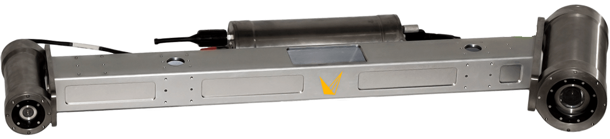
Figure 4: An Insight Pro underwater laser scanner developed by Voyis Imaging Inc. The beam emitter is on the left, while the camera is on the right. 3D point clouds are produced by triangulating the laser beam. The baseline between the emitter and the camera is approximately $1\text{\,}\mathrm{m}$.

III-A1 Point Cloud Generation

The Voyis Insight Pro underwater laser scanner, pictured in Figure 4, records 2D profile measurements of the seabed at a frequency of $20\text{\,}\mathrm{Hz}$. To construct a 3D point cloud, individual laser profiles are registered to the prior DVL-INS trajectory estimate $\check{\mbf{T}}^{z_{k}w}_{ab_{k}}$ via

$$\begin{bmatrix}\mbf{r}^{pw}_{a}\\ 1\end{bmatrix}=\check{\mbf{T}}^{z_{k}w}_{ab_{k}}\mbf{T}^{sz}_{b\ell}\begin{bmatrix}\mbf{r}^{ps_{k}}_{\ell_{k}}\\ 1\end{bmatrix},$$ (24)

where ${\mbf{r}^{ps_{k}}_{\ell_{k}}\in\mathbb{R}^{3}}$ is a laser measurement of point $p$ at time $t_{k}$ resolved in the sensor frame, and ${\mbf{T}^{sz}_{b\ell}\in SE(3)}$ is a static extrinsics matrix. Where necessary, the DVL-INS trajectory is interpolated according to [30, Sec. 2.4]

$$\check{\mbf{T}}_{j}= \ \check{\mbf{T}}_{i}\exp\left(\alpha\log\left(\check{\mbf{T}}^{-1}_{i}\check{\mbf{T}}_{k}\right)\right),$$ (25a)

$$\alpha= \ \frac{t_{j}-t_{i}}{t_{k}-t_{i}},$$ (25b)

where ${\check{\mbf{T}}_{j}=\check{\mbf{T}}^{z_{j}w}_{ab_{j}}}$, and ${t_{i}<t_{j}<t_{k}}$. The result of these operations is a filtered point cloud $\mathcal{P}$ resolved in the local geodetic frame, ${\mathcal{P}=\left\{\mbf{r}^{p_{i}w}_{a}\right\}^{N}_{i=1}}$.

III-A2 Point Cloud Alignment

The objective of point cloud alignment is to combine partially overlapping scans of the same 3D object or scene. In the context of SLAM, point cloud alignment is often performed to estimate the relative pose between two or more observations, for example to reduce odometry drift [31] or to bound navigation drift over time by closing large loops in the trajectory [32]. More formally, the problem of point cloud alignment may be expressed as

$$\mbf{T}^{\star}_{12}=\operatorname*{arg\,min}_{\mbf{T}\in SE(3)}\frac{1}{2}\sum^{N}_{i=1}\sum^{M}_{j=1}b_{ij}\cdot w_{ij}\cdot\left\|\mbf{e}_{ij}\left(\mbf{T}_{12},\mbf{r}^{p_{i}z_{2}}_{b_{2}},\mbf{r}^{p_{j}z_{1}}_{b_{1}}\right)\right\|^{2}_{\bm{\Sigma}^{-1}_{ij}},$$ (26)

where the pose ${\mbf{T}^{\star}_{12}=\left(\mbf{T}^{z_{2}z_{1}}_{b_{1}b_{2}}\right)^{\star}}$ optimally aligns source cloud ${\mathcal{S}=\{\mbf{r}^{p_{i}z_{2}}_{b_{2}}\}^{N}_{i=1}}$ to target cloud ${\mathcal{T}=\{\mbf{r}^{p_{j}z_{1}}_{b_{1}}\}^{M}_{j=1}}$. The Boolean value ${b_{ij}=\{0,1\}}$ assumes a value of 1 if $(p_{i},p_{j})$ represents an inlier correspondence, while ${w_{ij}\in[0,1]}$ is a correspondence weight, often computed using a robust cost function [33]. $\mbf{T}^{\star}_{12}$ is optimal in the sense that it minimizes the sum of squared weighted errors, often a combination of point-to-point and point-to-plane errors [34, 35], with associated error covariance ${\bm{\Sigma}_{ij}(\mbf{R}_{i},\mbf{R}_{j})}$. $\mbf{R}_{i}$ and $\mbf{R}_{j}$ represent the covariance on the point measurements $\mbf{r}^{p_{i}z_{2}}_{b_{2}}$ and $\mbf{r}^{p_{j}z_{1}}_{b_{1}}$, respectively, with ${\mbf{R}_{i}=\mathrm{E}[\delta\mbf{r}_{i}\,\delta\mbf{r}_{i}^{\mathsf{T}}]}$, ${\delta\mbf{r}_{i}=\mbf{r}^{p_{i}z_{2}}_{b_{2}}-\bar{\mbf{r}}^{p_{i}z_{2}}_{b_{2}}}$. A depiction of the point cloud alignment problem is shown in Figure 5.

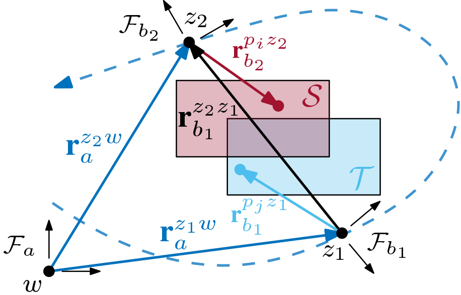
Figure 5: Generating a loop-closure measurement by aligning source submap $\mathcal{S}$ to target submap $\mathcal{T}$. The vehicle trajectory appears as a dashed line. Submaps ${\mathcal{T}=\{\mbf{r}^{p_{j}z_{1}}_{b_{1}}\}^{M}_{j=1}}$ and ${\mathcal{S}=\{\mbf{r}^{p_{i}z_{2}}_{b_{2}}\}^{N}_{i=1}}$ are constructed from the point measurements at vehicle poses $\mbf{T}^{z_{1}w}_{ab_{1}}$ and $\mbf{T}^{z_{2}w}_{ab_{2}}$, respectively. Point cloud alignment produces the loop-closure measurement $\mbf{T}^{z_{2}z_{1}}_{b_{1}b_{2}}$.

In this work, loop-closure locations are identified at simple path crossings on the $(x,y)$ plane, at time stamps $t_{\ell_{1}}$ and $t_{\ell_{2}}$, with ${t_{\ell_{1}}<t_{\ell_{2}}}$. Ordinarily, cross-covariance information would be used to determine the search region, and thus the required size of the submaps to construct, using a squared Mahalanobis distance test [36], however this information is absent from the DVL-INS trajectory estimate. Instead, given the inherently low drift rate of the DVL-INS [13], the source and target clouds are constructed using a simple $(x,y)$ distance threshold, e.g.

$$\mbf{r}^{pw}_{a}\in\mathcal{T}\,\big{|}\left\|\begin{bmatrix}\mbf{1}&\mbf{0}\end{bmatrix}\left(\mbf{r}^{pw}_{a}-{\check{\mbf{r}}_{a}}^{z_{\ell_{1}}w}\right)\right\|_{2}\leq\delta r^{\star}.$$ (27)

In this work a constant value of ${\delta r^{\star}=$5\text{\,}\mathrm{m}$}$ appears to work well, however a gradually increasing threshold related to the length of the trajectory could also be used.

To provide a body-frame relative pose measurement (26), the point measurements are first resolved in the body frames,

$$\begin{bmatrix}\mbf{r}^{pz_{\ell}}_{b_{\ell}}\\ 1\end{bmatrix}=\left(\check{\mbf{T}}^{z_{\ell}w}_{ab_{\ell}}\right)^{-1}\begin{bmatrix}\mbf{r}^{pw}_{a}\\ 1\end{bmatrix}.$$ (28)

The point clouds are preprocessed by downsampling to a $5\text{\,}\mathrm{cm}$ grid, which reduces the amount of point data by approximately a factor of 10 while still preserving high-frequency features of the scanned object. Normal vectors are then estimated using the 40 nearest Euclidean neighbours. To account for cases of large navigation drift between observations, the TEASER++ coarse alignment algorithm [37] is used to initialize an iterative closest point (ICP)-based fine alignment algorithm. To run TEASER++, FPFH feature descriptors [38] are computed at 3D SIFT keypoints [39], and a set of putative correspondences is formed from the 10 nearest neighbour matches in 33-dimensional FPFH space. Keypoints and descriptors are computed using the Point Cloud Library (PCL) v1.9 [40]. Default values are used for all TEASER++ parameters.

The combination of SIFT keypoints and FPFH descriptors was selected for this application following an alignment study on the shipwreck field dataset introduced in Section IV-D. In this dataset, a vehicle makes eight passes over a small shipwreck, producing eight point cloud submaps and 28 unique submap pairs. 27 of the 28 pairs were then aligned using TEASER++ and different detector/descriptor combinations, with one submap pair excluded due to insufficient overlap. The study includes three keypoint detectors and two 3D feature descriptors. The keypoint detectors are SIFT, ISS [41], and Harris 3D keypoints [42], while the feature descriptors are FPFH and SHOT [43]. These detectors and descriptors were included in the study both due to their prevalence in the point cloud alignment literature and the availability of an open-source implementation in PCL v1.9. SIFT and Harris 3D keypoint parameters were tuned slightly to obtain several hundred keypoints in each submap, while default values were used for ISS keypoints. For fairness, both FPFH and SHOT descriptors used the same search radius value of $0.25\text{\,}\mathrm{m}$.

TABLE I: Summary statistics from the keypoint detector and descriptor alignment study, reported in the format ${$50\text{\,}\mathrm{\char 37\relax}$\,\cdot\,\color[rgb]{0.45,0.45,0.45}{$90\text{\,}\mathrm{\char 37\relax}$}\color[rgb]{0,0,0}\,\cdot\,\color[rgb]{0.75,0.75,0.75}{\textrm{MAX}}\color[rgb]{0,0,0}}$. Attitude errors $\|\delta\bm{\phi}\|$ and position errors $\|\delta\bm{\rho}\|$ are computed according to (29). The lowest value in each column is indicated in bold font. Si = SIFT, I = ISS, H = Harris3D, F = FPFH, and So = SHOT.

KP	D	$\|\delta\bm{\phi}\|\,\left[\deg\right]$						$\|\delta\bm{\rho}\|\,\left[\operatorname{m}\right]$
Si	F	0.44	$\cdot$	1.05	$\cdot$	1.54		0.04	$\cdot$	0.09	$\cdot$	0.16
	So	0.42	$\cdot$	0.86	$\cdot$	92.59		0.03	$\cdot$	0.07	$\cdot$	3.33
I	F	0.49	$\cdot$	0.84	$\cdot$	52.34		0.04	$\cdot$	0.09	$\cdot$	2.31
	So	0.61	$\cdot$	176.28	$\cdot$	179.72		0.05	$\cdot$	20.12	$\cdot$	22.56
H	F	0.83	$\cdot$	21.14	$\cdot$	178.44		0.08	$\cdot$	3.05	$\cdot$	22.48
	So	0.83	$\cdot$	52.32	$\cdot$	164.84		0.06	$\cdot$	4.22	$\cdot$	18.28

Each submap pair was then aligned by TEASER++ using each of the six detector/descriptor combinations. The results are given in Table I, which lists summary statistics on attitude errors $\|\delta\bm{\phi}\|$ and position errors $\|\delta\bm{\rho}\|$ in the format ${$50\text{\,}\mathrm{\char 37\relax}$\,\cdot\,\color[rgb]{0.45,0.45,0.45}{$90\text{\,}\mathrm{\char 37\relax}$}\color[rgb]{0,0,0}\,\cdot\,\color[rgb]{0.75,0.75,0.75}{\textrm{MAX}}\color[rgb]{0,0,0}}$. Pose errors were computed between each TEASER++ relative pose estimate $\tilde{\mbf{T}}_{i}$ and the ground-truth relative pose $\mbf{T}_{i}$, computed from a well-initialized ICP alignment, as

$$\delta\bm{\xi}_{i}=\log(\mbf{T}_{i}^{-1}\tilde{\mbf{T}}_{i})^{\vee}.$$ (29)

Examining Table I, the combination of SIFT keypoints and SHOT descriptors (second row) delivers the lowest median attitude error ($0.42\text{\,}\deg$), as well as the lowest $50\text{\,}\mathrm{\char 37\relax}$ and $90\text{\,}\mathrm{\char 37\relax}$ position errors. However, this combination produced at least one outlier measurement from the 27 submap pairs, while the SIFT+FPFH combination (first row) produced zero outliers. In addition, the SIFT+FPFH combination produced reasonable median and $90\text{\,}\mathrm{\char 37\relax}$ errors. Note the extremely large position errors in Table I are due to failed alignments producing a $180\text{\,}\deg$ “flip” of the (relatively flat) point cloud submaps. The submaps are measured at a range of approximately $7\text{\,}\mathrm{m}$, thus “flipped” alignments produce a relative body-frame position error of more than twice this value.

As the objective of a coarse alignment algorithm is to robustly initialize ICP as close to ground-truth as possible, the SIFT+FPFH combination was selected for this application. Note that TEASER++ was chosen for the coarse alignment algorithm as it has been shown in extensive point cloud alignment studies [37] to outperform other coarse alignment methods, for example FGR [44] and RANSAC [45].

For the fine alignment step, this work uses the Weighted Optimal Linear Attitude and Translation Estimator (WOLATE) algorithm [46] within an ICP-based alignment scheme. Alignment errors are formulated between each point in the source cloud and their single nearest neighbour in the target cloud. A combination of point-to-point and point-to-plane errors are used, with the surface variation $v(p_{j})$ [47] of the target points determining the type of error used for each association. Following the study in [48], the Fractional Root Mean Squared Distance (FRMSD) robust cost function [49] is used for outlier rejection when aligning structured scans, such as shipwrecks. The algorithm terminates when the pose differential $\delta\bm{\xi}_{i}$ between two successive iterations falls below a threshold, or when a maximum number of iterations is reached. Following the recommendations in [50] for best practices when reporting ICP algorithms, the preprocessing steps and relevant parameters are summarized in Table II.

TABLE II: ICP preprocessing and alignment parameters

Stage	Configuration	Description
Preprocessing	VoxelGrid	Downsample to $5\text{\,}\mathrm{cm}$ grid
	Normals	40 nearest neighbours
Keypoints	3D SIFT	PCL v1.9 implementation
Descriptors	FPFH	PCL v1.9 implementation
Coarse align.	TEASER++	10 matches, default params.
ICP data assn.	KDTree	Single nearest neighbour
ICP error min.	Mixed	Pt-Pl if $v(p_{j})<$310-2\text{\,}$$
Outlier reject.	FRMSD	Default params. from [49]
Termination	Diff.	${\|\delta\bm{\phi}_{i}\|_{2}<$110-2\text{\,}\mathrm{rad}$}$, and ${\|\delta\bm{\rho}_{i}\|_{2}<$110-3\text{\,}\mathrm{m}$}$
	Counter	20 iterations max

III-A3 Loop-Closure Measurement Model

Point cloud alignment yields the loop-closure measurement

$$\bm{\Xi}_{\ell_{1}\ell_{2}}\triangleq\mbf{T}^{z_{\ell_{2}}z_{\ell_{1}}}_{b_{\ell_{1}}b_{\ell_{2}}}=\left(\mbf{T}^{z_{\ell_{1}}w}_{ab_{\ell_{1}}}\right)^{-1}\mbf{T}^{z_{\ell_{2}}w}_{ab_{\ell_{2}}}\in SE(3),$$ (30)

and, given the perturbation scheme (11), the noise model is

$$\bm{\Xi}_{\ell_{1}\ell_{2}}= \ \mbf{g}_{\ell}(\check{\mbf{T}}_{\ell_{1}},\check{\mbf{T}}_{\ell_{2}},\delta\bm{\xi}_{\Xi})$$ (31a)

$$= \ \bar{\bm{\Xi}}_{\ell_{1}\ell_{2}}\exp(-\delta\bm{\xi}^{\wedge}_{\Xi}),$$ (31b)

$$\delta\bm{\xi}_{\Xi}\sim \ \mathcal{N}(\mbf{0},\mbf{R}_{\Xi}),$$ (31c)

where the shorthand ${\check{\mbf{T}}_{\ell_{i}}=\check{\mbf{T}}^{z_{\ell_{i}}w}_{ab_{\ell_{i}}},i=1,2}$ is used for readability. The covariance $\mbf{R}_{\Xi}$ on the loop-closure measurement may be obtained from the point cloud alignment algorithm in a number of ways, for example the linearization-based approach in [51].

III-B Updating the Trajectory

III-B1 Formulating the Objective Function

The objective is now to condition the prior DVL-INS trajectory estimate on the newly available loop-closure measurements. This is accomplished through nonlinear batch state estimation, described in Section II-E. This section describes how the error terms in the batch problem are formulated, and Figure 6 shows the resulting factor graph.

First, the prior, process, and measurement errors must be defined. Given the augmented navigation state (19), errors must be defined for the $SE(3)$ pose and for the generalized velocity. Using both the left-invariant error definition (10) and the constant velocity WNOA motion prior, the prior error is

$$\mbf{e}_{0}=\begin{bmatrix}\mbf{e}^{\xi}_{0}\\ \mbf{e}^{\varpi}_{0}\end{bmatrix}=\begin{bmatrix}\log\left(\mbf{T}_{0}^{-1}\mbf{Y}_{0}\right)^{\vee}\\ \bm{\varpi}_{0}-\bm{\psi}_{0}\end{bmatrix},$$ (32)

where ${(\mbf{Y}_{0},\bm{\psi}_{0})}$ is the prior estimate on the first navigation state. The process errors take the form

$$\mbf{e}_{k}=\begin{bmatrix}\mbf{e}^{\xi}_{k}\\ \mbf{e}^{\varpi}_{k}\end{bmatrix}=\begin{bmatrix}\log\left(\mbf{T}_{k}^{-1}\tilde{\mbf{T}}_{k}\right)^{\vee}\\ \bm{\varpi}_{k}-\bm{\varpi}_{k-1}\end{bmatrix},$$ (33)

where the predicted pose at time $t_{k}$,

$$\tilde{\mbf{T}}_{k}=\mbf{f}_{k-1}(\mbf{T}_{k-1},\bm{\varpi}_{k-1})=\mbf{T}_{k-1}\exp(T\bm{\varpi}^{\wedge}_{k-1}),$$ (34)

arises from a forward Euler discretization of the continuous-time $SE(3)$ kinematics (18a) over an integration period of ${T=t_{k}-t_{k-1}}$. The loop-closure errors are

$$\mbf{e}_{\ell}=\mbf{T}_{\ell_{2}}^{-1}\tilde{\mbf{T}}_{\ell_{2}}=\mbf{T}_{\ell_{2}}^{-1}\mbf{T}_{\ell_{1}}\bm{\Xi}_{\ell_{1}\ell_{2}},$$ (35)

where $\mbf{T}_{\ell_{1}}$ and $\mbf{T}_{\ell_{2}}$ are the two poses involved in loop-closure measurement $\ell$. Additionally, it was discovered in testing that including a relative pose constraint between each subsequent pair of poses helped the loop-closure correction to propagate throughout the trajectory. The relative pose errors take the same form as the loop-closure errors,

$$\mbf{e}^{\textrm{rel.}}_{k}=\mbf{T}_{k}^{-1}\tilde{\mbf{T}}_{k}=\mbf{T}_{k}^{-1}\mbf{T}_{k-1}\bm{\Xi}_{k-1,k},\vspace{-1pt}$$ (36)

where the relative pose measurements are taken directly from the initializing solution,

$$\bm{\Xi}_{k-1,k}=\check{\mbf{T}}^{-1}_{k-1}\check{\mbf{T}}_{k}.\vspace{-1pt}$$ (37)

Finally, since roll, pitch, and depth are directly observable AUV states [5], errors are included of the form

$$\mbf{e}^{\textrm{obs.}}_{k}=\begin{bmatrix}e^{\phi_{1}}_{k}\\ e^{\phi_{2}}_{k}\\ e^{\textrm{z}}_{k}\end{bmatrix}=\mbf{D}\mbf{E}_{k}\log\left(\mbf{T}_{k}^{-1}\check{\mbf{T}}_{k}\right)^{\vee},\vspace{-3pt}$$ (38)

where

$$\mbf{D}=\begin{bmatrix}\mbf{1}&\mbf{0}&\mbf{0}\\ \mbf{0}&\mbf{0}&1\end{bmatrix}\in\mathbb{R}^{3\times 6},\quad\mbf{E}_{k}=\begin{bmatrix}\mbf{1}&\\ &\mbf{C}_{ab_{k}}\mbf{J}^{\ell}(\mbf{e}^{\phi}_{k})\end{bmatrix},$$ (39)

where $\mbf{J}^{\ell}$ is the left Jacobian of $SO(3)$ [23, Sec. 7.1.3], and

$$\mbf{e}^{\xi}_{k}=\begin{bmatrix}(\mbf{e}^{\phi}_{k})^{\mathsf{T}}&(\mbf{e}^{\rho}_{k})^{\mathsf{T}}\end{bmatrix}^{\mathsf{T}}.$$ (40)

The least-squares objective function (23) is then augmented as

$$J_{\textrm{aug.}}(\mbf{X})=J(\mbf{X})+\frac{1}{2}\sum_{k=1}^{K}\left(\big{\|}\mbf{e}^{\textrm{rel.}}_{k}\big{\|}^{2}_{\mbf{R}^{-1}_{\textrm{rel.}}}+\big{\|}\mbf{e}^{\textrm{obs.}}_{k}\big{\|}^{2}_{\mbf{R}^{-1}_{\textrm{obs.}}}\right),$$ (41)

where $\mbf{R}_{\textrm{rel.}}$ and $\mbf{R}_{\textrm{obs.}}$ are considered to be additional hyperparameters. Together, the relative pose errors (36) promote loop-closure propagation, while the WNOA errors (33) promote smoothing. The hyperparameters $\bm{\mathcal{Q}}$ and $\mbf{R}_{\textrm{rel.}}$ may be tuned to control the smoothness of the posterior solution, while $\mbf{R}_{\textrm{obs.}}$ is tuned to ensure the posterior does not stray too far in observable dimensions.

The batch estimation problem is visualized in the factor graph of Figure 6. Note that, in contrast to the initial factor graph in Figure 2, there are now factors linking adjacent nodes. This will allow corrections from the loop-closure measurements to propagate throughout the pose graph, as required.

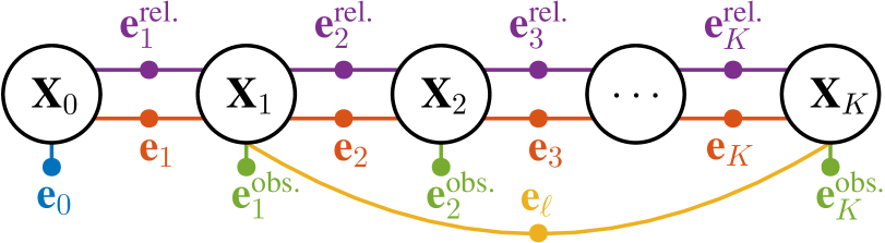
Figure 6: The factor graph corresponding to the batch state estimation problem. The formation of WNOA factors $\mbf{e}_{k}$ and relative pose factors $\mbf{e}^{\textrm{rel.}}_{k}$ allow corrections from loop-closure factor $\mbf{e}_{\ell}$ to propagate throughout the graph.

III-B2 Minimizing the Objective Function

To minimize (41), the estimation errors are repeatedly linearized about the current navigation state estimate $\bar{\mbf{X}}$. Perturbing the navigation state as

$$\mbf{T}= \ \bar{\mbf{T}}\exp(-\delta\bm{\xi}^{\wedge}),$$ (42a)

$$\bm{\varpi}= \ \bar{\bm{\varpi}}+\delta\bm{\varpi},$$ (42b)

$$\delta\mbf{x}= \begin{bmatrix}\delta\bm{\xi}^{\mathsf{T}}&\delta\bm{\varpi}^{\mathsf{T}}\end{bmatrix}^{\mathsf{T}},$$ (42c)

the prior error (32) is linearized as

$$\mbf{e}_{0}=\bar{\mbf{e}}_{0}+\mbf{F}_{0}^{0}\delta\mbf{x}_{0}+\mbf{M}_{0}\delta\mbf{y}_{0},$$ (43)

where ${\delta\mbf{y}_{0}=\begin{bmatrix}\delta\bm{\eta}_{0}^{\mathsf{T}}&\delta\bm{\psi}_{0}^{\mathsf{T}}\end{bmatrix}^{\mathsf{T}}}$, ${\mbf{S}_{0}=\mathrm{E}[\delta\mbf{y}_{0}\,\delta\mbf{y}_{0}^{\mathsf{T}}]}$, and where the prior Jacobians are

$$\mbf{F}_{0}^{0}= \ \operatorname{blkdiag}(\mbf{J}^{\ell}(\bar{\mbf{e}}^{\xi}_{0})^{-1},\mbf{1}),$$ (44a)

$$\mbf{M}_{0}= \ \operatorname{blkdiag}(-\mbf{J}^{\textrm{r}}(\bar{\mbf{e}}^{\xi}_{0})^{-1},-\mbf{1}),$$ (44b)

with $\mbf{J}^{\ell}$ being the left Jacobian of $SE(3)$. Note that detailed derivations of the work appearing in this section are available in the supplementary material in Appendix A. The discrete-time process errors (33) are linearized as

$$\mbf{e}_{k}=\bar{\mbf{e}}_{k}+\color[rgb]{0,0,0}{\mbf{F}^{k}_{k-1}}\color[rgb]{0,0,0}\delta\mbf{x}_{k-1}+\color[rgb]{0,0,0}{\mbf{F}^{k}_{k}}\color[rgb]{0,0,0}\delta\mbf{x}_{k},$$ (45)

where the process error Jacobians are given by

$$\mbf{F}^{k}_{k-1}= \begin{bmatrix}\mbf{U}_{k-1}&\mbf{V}_{k-1}\\ \mbf{0}&-\mbf{1}\end{bmatrix},$$ (46a)

$$\mbf{U}_{k-1}= \ -\mbf{J}^{\textrm{r}}(\bar{\mbf{e}}^{\xi}_{k})^{-1}\operatorname{\mbf{Ad}}(\exp(-T\bar{\bm{\varpi}}_{k-1}^{\wedge})),$$

$$\mbf{V}_{k-1}= \ T\mbf{J}^{\textrm{r}}(\bar{\mbf{e}}^{\xi}_{k})^{-1}\mbf{J}^{\textrm{r}}(T\bar{\bm{\varpi}}_{k-1}),$$

$$\mbf{F}^{k}_{k}= \begin{bmatrix}\mbf{J}^{\ell}(\bar{\mbf{e}}^{\xi}_{k})^{-1}&\mbf{0}\\ \mbf{0}&\mbf{1}\end{bmatrix}.$$ (46b)

The loop-closure errors (35) are linearized as

$$\mbf{e}_{\ell}=\bar{\mbf{e}}_{\ell}+\mbf{H}^{\ell}_{\ell_{1}}\delta\bm{\xi}_{\ell_{1}}+\mbf{H}^{\ell}_{\ell_{2}}\delta\bm{\xi}_{\ell_{2}}+\mbf{M}_{\ell}\delta\bm{\xi}_{\Xi},$$ (47)

with corresponding Jacobians

$$\mbf{H}^{\ell}_{\ell_{1}}= \ -\mbf{J}^{\textrm{r}}(\bar{\mbf{e}}_{\ell})^{-1}\operatorname{\mbf{Ad}}(\bar{\bm{\Xi}}_{\ell_{1}\ell_{2}}^{-1}),$$ (48a)

$$\mbf{H}^{\ell}_{\ell_{2}}= \ \mbf{J}^{\ell}(\bar{\mbf{e}}_{\ell})^{-1},$$ (48b)

$$\mbf{M}_{\ell}= \ -\mbf{J}^{\textrm{r}}(\bar{\mbf{e}}_{\ell})^{-1}.$$ (48c)

The relative pose errors (36) are linearized in the same manner. Finally, errors on the observable states (38) are linearized by approximating

$$\mbf{C}_{ab_{k}}=\bar{\mbf{C}}_{ab_{k}}\exp\left(-\delta\bm{\phi}_{k}^{\times}\right)\approx\bar{\mbf{C}}_{ab_{k}}\left(\mbf{1}-\delta\bm{\phi}_{k}^{\times}\right).\vspace{-2pt}$$ (49)

Assuming ${\mbf{e}^{\rho}_{k}\to\mbf{0}}$ as the optimization proceeds, this yields

$$\mbf{e}^{\textrm{obs.}}_{k}= \ \bar{\mbf{e}}^{\textrm{obs.}}_{k}+\mbf{H}^{\textrm{obs.}}_{k}\delta\bm{\xi}_{k},$$ (50)

$$\mbf{H}^{\textrm{obs.}}_{k}= \ \mbf{D}\mbf{E}_{k}(\bar{\mbf{C}}_{ab_{k}},\bar{\mbf{e}}^{\phi}_{k})\mbf{J}^{\ell}(\bar{\mbf{e}}^{\xi}_{k})^{-1}.\vspace{-2pt}$$ (51)

The final step is to determine the covariance on the discrete-time WNOA process errors. This is done by discretizing the power spectral density $\bm{\mathcal{Q}}$ via [52, (4.110)]

$$\mbf{Q}_{k}=\int^{t_{k}}_{t_{k-1}}\mbf{A}(t_{k},s)\mbf{L}(s)\bm{\mathcal{Q}}(s)\left(\mbf{A}(t_{k},s)\mbf{L}(s)\right)^{\mathsf{T}}\mathrm{d}s,\vspace{-2pt}$$ (52)

where ${\mbf{A},\mbf{L}}$ characterize the continuous-time error kinematics, which for the WNOA motion prior take the form

$$\delta\dot{\mbf{x}}(t)=\underbrace{\begin{bmatrix}-\operatorname{\mbf{ad}}(\bar{\bm{\varpi}}^{\wedge})&-\mbf{1}\\ \mbf{0}&\mbf{0}\end{bmatrix}}_{\mbf{A}}\delta\mbf{x}(t)+\underbrace{\begin{bmatrix}\mbf{0}\\ \mbf{1}\end{bmatrix}}_{\mbf{L}}\delta\mbf{w}(t),$$ (53)

with ${\delta\mbf{w}(t)\sim\mathcal{GP}(\mbf{0},\bm{\mathcal{Q}}(t-t^{\prime}))}$. The exact solution to (52) may be obtained via the matrix exponential [53], however to avoid this expensive operation this work makes use of a third-order approximation in $\mbf{A}$ [52, (4.119)],

$$\mbf{Q}_{k} \approx T\bm{\Upsilon}+\frac{T^{2}}{2}\left(\mbf{A}\bm{\Upsilon}+\bm{\Upsilon}\mbf{A}^{\mathsf{T}}\right)$$

$$+\frac{T^{3}}{6}\left(\mbf{A}^{2}\bm{\Upsilon}+2\mbf{A}\bm{\Upsilon}\mbf{A}^{\mathsf{T}}+\bm{\Upsilon}\left(\mbf{A}^{\mathsf{T}}\right)^{2}\right)$$ (54)

$$+\frac{T^{4}}{24}\left(\mbf{A}^{3}\bm{\Upsilon}+3\mbf{A}^{2}\bm{\Upsilon}\mbf{A}^{\mathsf{T}}+3\mbf{A}\bm{\Upsilon}\left(\mbf{A}^{\mathsf{T}}\right)^{2}+\bm{\Upsilon}\left(\mbf{A}^{\mathsf{T}}\right)^{3}\right),\vspace{-4pt}$$

where ${\bm{\Upsilon}=\mbf{L}\bm{\mathcal{Q}}\mbf{L}^{\mathsf{T}}}$. Finally, the minimizing solution for a single iteration of Gauss-Newton is

$$\delta\mbf{x}_{\star}=\begin{bmatrix}\delta\bm{\xi}_{\star}\\ \delta\bm{\varpi}_{\star}\end{bmatrix}=-\left(\bm{\Gamma}^{\mathsf{T}}\mbf{W}\bm{\Gamma}\right)^{-1}\bm{\Gamma}^{\mathsf{T}}\mbf{W}\mbf{e}.$$ (55)

Jacobian $\bm{\Gamma}$ is given by

$$\bm{\Gamma}= \begin{bmatrix}\mbf{F}^{\mathsf{T}}&\mbf{H}^{\mathsf{T}}&{\mbf{H}^{\textrm{rel.}}}^{\mathsf{T}}&{\mbf{H}^{\textrm{obs.}}}^{\mathsf{T}}\end{bmatrix}^{\mathsf{T}},$$ (56)

$$\mbf{F}= \begin{bmatrix}\mbf{F}^{0}_{0}&&&\\ \mbf{F}^{1}_{0}&\mbf{F}^{1}_{1}&&\\ &\ddots&\ddots&\\ &&\mbf{F}^{K}_{K-1}&\mbf{F}^{K}_{K}\end{bmatrix},$$ (57)

$$\mbf{H}= \begin{bmatrix}&\mbf{H}^{1}_{\ell_{1}}&&&\mbf{H}^{1}_{\ell_{2}}&\\ &&&\vdots&&\\ &&\mbf{H}^{L}_{\ell_{1}}&&&\mbf{H}^{L}_{\ell_{2}}\end{bmatrix},$$ (58)

$$\mbf{H}^{\textrm{rel.}}= \begin{bmatrix}\mbf{H}^{\textrm{rel.},1}_{0}&\mbf{H}^{\textrm{rel.},1}_{1}&&\\ &\ddots&\ddots&\\ &&\mbf{H}^{\textrm{rel.},K}_{K-1}&\mbf{H}^{\textrm{rel.},K}_{K}\end{bmatrix},$$ (59)

$$\mbf{H}^{\textrm{obs.}}= \begin{bmatrix}\mbf{0}&\mbf{H}^{\textrm{obs.}}_{1}&&\\ &&\ddots&\\ &&&\mbf{H}^{\textrm{obs.}}_{K}\end{bmatrix},$$ (60)

and weighting matrix ${\mbf{W}=\bm{\Sigma}^{-1}}$ is described by

$$\bm{\Sigma}=\operatorname{blkdiag}\left(\mbf{M}_{0}\mbf{S}_{0}\mbf{M}_{0}^{\mathsf{T}},\mbf{Q}_{1:K},\mbf{R}_{1:L},\mbf{R}^{\textrm{rel.}}_{1:K},\mbf{R}^{\textrm{obs.}}_{1:K}\right),\vspace{6pt}$$ (61)

where, for the loop-closure errors,

$$\mbf{R}_{\ell}=\mbf{M}_{\ell}\mbf{R}_{\Xi}\mbf{M}_{\ell}^{\mathsf{T}}.\vspace{3pt}$$ (62)

The column matrix of errors is simply

$$\mbf{e}=\begin{bmatrix}\mbf{e}_{0}^{\mathsf{T}}&\mbf{e}_{1:K}^{\mathsf{T}}&\mbf{e}_{1:L}^{\mathsf{T}}&\left(\mbf{e}^{\textrm{rel.}}_{1:K}\right)^{\mathsf{T}}&\left(\mbf{e}^{\textrm{obs.}}_{1:K}\right)^{\mathsf{T}}\end{bmatrix}^{\mathsf{T}}.\vspace{6pt}$$ (63)

Finally, in accordance with the perturbation scheme (42a, 42b), the state update is given by

$$\mbf{T}\leftarrow \ \mbf{T}\exp(-\delta\bm{\xi}^{\wedge}_{\star}),$$ (64a)

$$\bm{\varpi}\leftarrow \ \bm{\varpi}+\delta\bm{\varpi}_{\star}.$$ (64b)

III-B3 Rejecting False Loop-Closure Measurements

Measurement outliers are inevitable in real-world robotics problems, and a robust implementation of the proposed methodology requires a method to identify and reject false loop-closure measurements. Many approaches exist in the literature for rejecting loop-closure measurement outliers, for example switchable constraints [54], expectation-maximization [55], and graduated non-convexity [56].

This application uses a recently developed adaptive robust cost function (RCF) to reject false loop-closure measurements, owing to its ability to handle multivariate, mixed-unit error definitions, such as loop-closure errors (35), in a statistically sound manner [57]. The RCF assigns a weight ${w_{\ell}(\epsilon_{\ell}(\mbf{e}_{\ell}))\in(0,1]}$ to loop-closure error $\mbf{e}_{\ell}$ according to the Mahalanobis distance associated with the error,

$$\epsilon_{\ell}(\mbf{e}_{\ell})=\|\mbf{e}_{\ell}\|_{\bm{\Sigma}_{\ell}^{-1}}\in\mathbb{R}_{\geq 0},\vspace{3pt}$$ (65)

where, ordinarily, the covariance $\bm{\Sigma}_{\ell}$ on the (relative) loop-closure measurement would be the relative uncertainty computed between the two vehicle poses involved in the measurement [58]. Since the DVL-INS output does not contain the joint covariance information required to properly compute $\bm{\Sigma}_{\ell}$, a constant value is used here,

$$\bm{\Sigma}_{\ell}=\operatorname{blkdiag}(\sigma^{2}_{\phi_{\textrm{out}}}\mbf{1},\sigma^{2}_{\rho_{\textrm{out}}}\mbf{1}),\vspace{3pt}$$ (66)

with ${\sigma_{\phi_{\textrm{out}}}=$1\text{\,}\deg$}$ and ${\sigma_{\rho_{\textrm{out}}}=$1\text{\,}\mathrm{m}$}$. These $1\sigma$ values reflect the low heading uncertainty of the survey-grade DVL-INS used in the field experiments, as well as the static search bound used for the loop-closure detection method (27).

IV Results

IV-A Assessing the Quality of the State Estimate

The methodology described in Section III conditions an existing state estimate on newly available loop-closure measurements. Since loop closures provide relative constraints between poses, as shown in Figure 6, it is expected that this approach will

1. reduce relative pose errors throughout the trajectory; and

2. produce a more self-consistent point cloud map, as measured by a reduction in the point disparity error in overlapping regions.

IV-A1 Measuring Errors in the Estimated Trajectory

A pose-based relative error metric based on [59] is used to measure the accuracy of the estimated trajectory. Let ${\hat{\mbf{T}}_{k}\in SE(3)}$ represent the estimated pose at time $t_{k}$. The pose at time $t_{k}$ relative to the pose at time $t_{\ell}$ is

$$\delta\hat{\mbf{T}}_{\ell k}=\hat{\mbf{T}}^{-1}_{\ell}\hat{\mbf{T}}_{k},\vspace{-2pt}$$ (67)

where $\hat{\mbf{T}}_{\ell}$ is taken to be the earliest pose involved in any loop-closure measurement. The relative pose error may then be expressed as

$$\mbf{E}^{\textrm{rel.}}_{k}=\delta\mbf{T}^{-1}_{\ell k}\delta\hat{\mbf{T}}_{\ell k}=\begin{bmatrix}\delta\mbf{C}_{k}&\delta\mbf{r}_{k}\\ \mbf{0}&1\end{bmatrix},\vspace{-1pt}$$ (68)

where $\delta\mbf{T}_{\ell k}$ is (67) evaluated using the ground-truth trajectory. Relative pose errors on $SE(3)$ may then be expressed in the Lie algebra as

$$\color[rgb]{0,0,0}{\delta\mbf{e}^{\textrm{rel.}}_{k}=\log\left(\mbf{E}^{\textrm{rel.}}_{k}\right)^{\vee}=\begin{bmatrix}(\delta\bm{\phi}^{\textrm{rel.}}_{k})^{\mathsf{T}}\ (\delta\bm{\rho}^{\textrm{rel.}}_{k})^{\mathsf{T}}\end{bmatrix}^{\mathsf{T}}.}\color[rgb]{0,0,0}$$ (69)

However, since the AUV trajectories studied in this work are largely planar, the accuracy of the trajectory estimate is reported as the norm of the relative displacement error $\delta\mbf{r}_{k}$ projected on the $(x,y)$ plane,

$$e^{\textrm{rel.}}_{k}=\left\|\begin{bmatrix}\mbf{1}&\mbf{0}\end{bmatrix}\delta\mbf{r}_{k}\right\|_{2}.\vspace{-2pt}$$ (70)

Assessing performance using a relative metric such as (68) avoids the problem of aligning the estimated and ground-truth trajectories, which would be required if attempting to provide an absolute performance metric [59]. In addition to being intuitive and easy to visualize, the relative planar displacement metric (70) allows for direct comparison to other navigation solutions within the subsea industry, where position drift is often reported on the $(x,y)$ plane as a percentage of distance traveled. For estimates incorporating multiple loop closures along the length of the trajectory, the relative displacement error (70) is expected to remain bounded over time.

IV-A2 Measuring Self-Consistency in the Point Cloud Map

Performance is also assessed by evaluating the self-consistency in overlapping regions of the point cloud map. A point cloud map generated from an accurate trajectory estimate is expected to be well-aligned, or “crisp.” In contrast, a map produced using a drifting trajectory estimate will see “double vision” effects in overlapping regions due to poorly aligned scans. To assess self-consistency in the point cloud map, this work uses the point disparity metric from [60]. For point clouds ${\mathcal{S}=\{\mbf{r}^{p_{i}w}_{a}\}^{N}_{i=1}}$ and ${\mathcal{T}=\{\mbf{r}^{p_{j}w}_{a}\}^{M}_{j=1}}$, this metric is

$$e^{\textrm{rel.}}_{j}=\left\|\mbf{r}^{p_{j}w}_{a}-\mbf{r}^{p_{i}w}_{a}\right\|_{2},\vspace{-1pt}$$ (71)

where point $p_{j}$ in $\mathcal{T}$ is the nearest Euclidean neighbour to point $p_{i}$ in $\mathcal{S}$. Note (71) is only computed within the intersection of $\mathcal{S}$ and $\mathcal{T}$ to prevent cloud size from biasing the metric. The point disparity metric is relative, and may be computed without access to ground-truth information [60], making it especially important for field trials where a ground-truth map is not available. Note the point disparity metric is susceptible to map-to-map error, whereby an erroneous group of two or more well-aligned submaps would produce low disparity errors, despite separation from the true submap group. The results in the following studies were visually checked to ensure the absence of this error, though extending (71) to account for map-to-map error is an interesting avenue for future research.

IV-B Hyperparameter Values

The methodology described in Section III involves three sets of hyperparameters. These are

1. $\bm{\mathcal{Q}}$, the PSD on the white noise Gaussian process;

2. $\mbf{R}^{\textrm{rel.}}_{k}$, the covariance on the relative pose errors; and

3. $\mbf{R}^{\textrm{obs.}}_{k}$, the covariance on the roll, pitch, and depth errors, all of which are assumed to be observable.

The hyperparameter sets take the form

$$\bm{\mathcal{Q}}= \ {\mathrm{diag}}(\mathcal{Q}_{\dot{\omega}}\mbf{1},\mathcal{Q}_{\dot{\nu}}\mbf{1}),$$ (72a)

$$\mbf{R}^{\textrm{rel.}}_{k}= \ {\mathrm{diag}}(\sigma^{2}_{\phi}\mbf{1},\sigma^{2}_{\rho}\mbf{1}),$$ (72b)

$$\mbf{R}^{\textrm{obs.}}_{k}= \ {\mathrm{diag}}(\sigma^{2}_{\textrm{rp}}\mbf{1},\sigma^{2}_{\textrm{z}}),$$ (72c)

where $\mathcal{Q}_{\dot{\omega}}$, $\mathcal{Q}_{\dot{\nu}}$ are the power spectral densities on the body-centric angular and linear acceleration, respectively, and $\sigma^{2}_{\phi}$, $\sigma^{2}_{\rho}$ are the variances on the body-centric angular and linear displacement, respectively. $\sigma^{2}_{\textrm{rp}}$ is the variance on vehicle roll and pitch, and $\sigma^{2}_{\textrm{z}}$ is the variance on vehicle depth. While this hyperparameter structure is simple, it was found to work well for both simulated and field experiments, and generally makes physical sense. For example, [61] scales the values of a diagonal $\bm{\mathcal{Q}}$ matrix to reflect the nonholonomic constraints of an automobile. In contrast, AUVs are highly maneuverable, leading to the selection of isotropic hyperparameters in (72).

This section contains results from both simulated and field experiments. The hyperparameter values used to obtain each set of results are summarized in Table III. These values were hand-selected to produce good results without extensive tuning, and were modified based on the quality of the DVL-INS state estimate and the frequency at which DVL-INS data were available.

TABLE III: Hyperparameter values used in experiments

Hyperparameter	Unit	Simulated	Field
$\mathcal{Q}_{\dot{\omega}}$	$\text{\,}{\mathrm{rad}}^{2}\text{\,}{\mathrm{s}}^{-3}$	$110-2\text{\,}$	$110-2\text{\,}$
$\mathcal{Q}_{\dot{\nu}}$	$\text{\,}{\mathrm{m}}^{2}\text{\,}{\mathrm{s}}^{-3}$	$910-4\text{\,}$	$110-4\text{\,}$
$\sigma_{\phi}$	$\text{\,}\mathrm{rad}$	$110-3\text{\,}$	$110-3\text{\,}$
$\sigma_{\rho}$	$\text{\,}\mathrm{m}$	$110-4\text{\,}$	$110-3\text{\,}$
$\sigma_{\textrm{rp}}$	$\text{\,}\deg$	5	5
$\sigma_{\textrm{z}}$	$\text{\,}\mathrm{m}$	0.25	0.25

IV-C Simulation Results: AUV Area Inspection

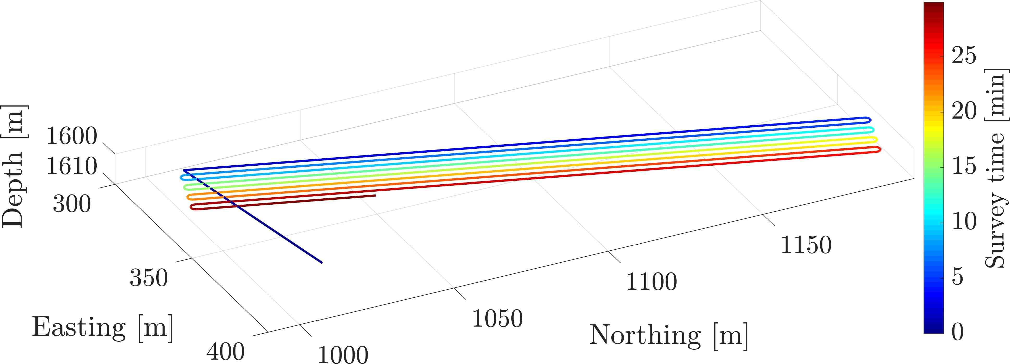
Figure 7: The simulated dataset. A single tie-line is intersected on the left by multiple “lawnmower” inspection passes.

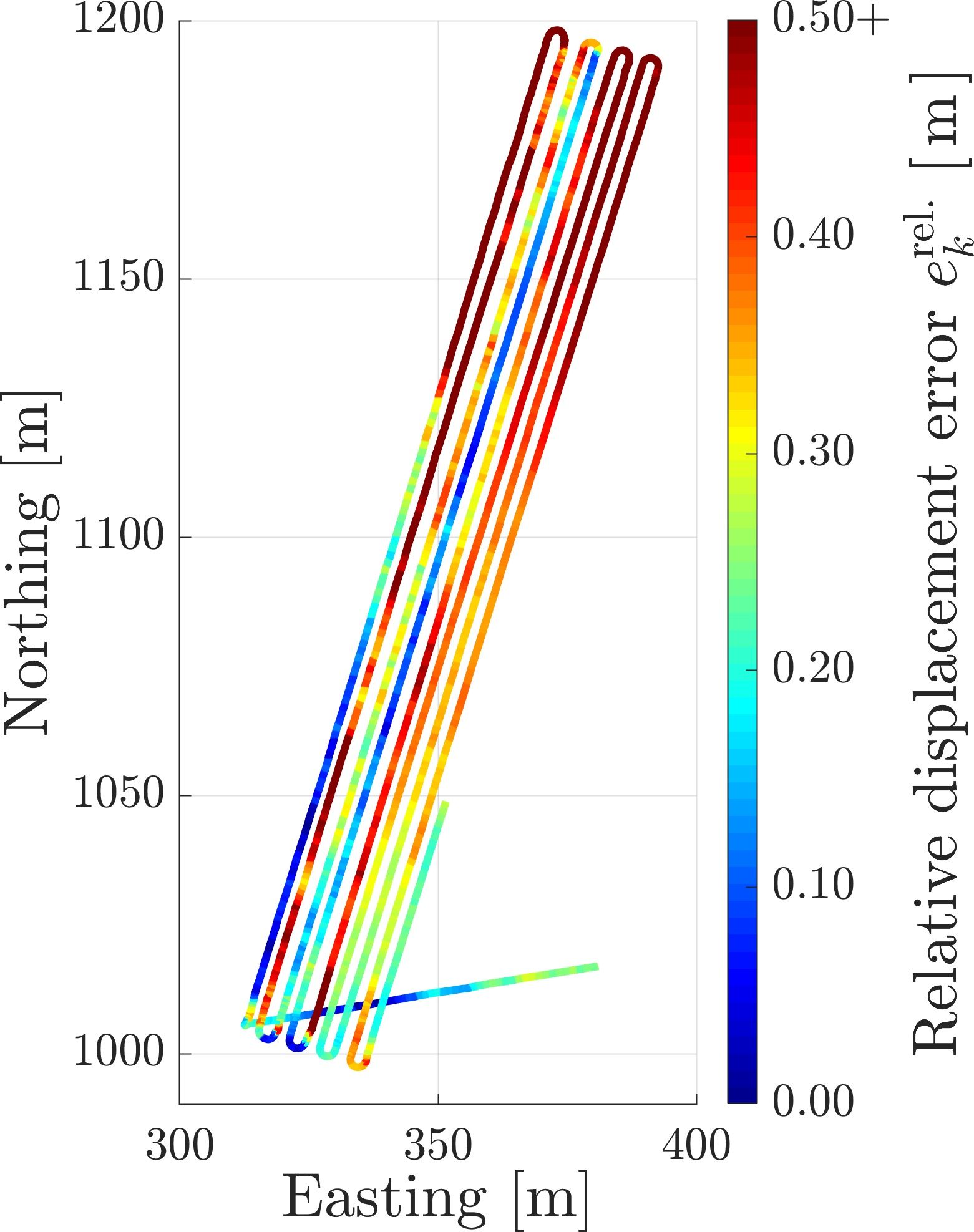
(a) INS top

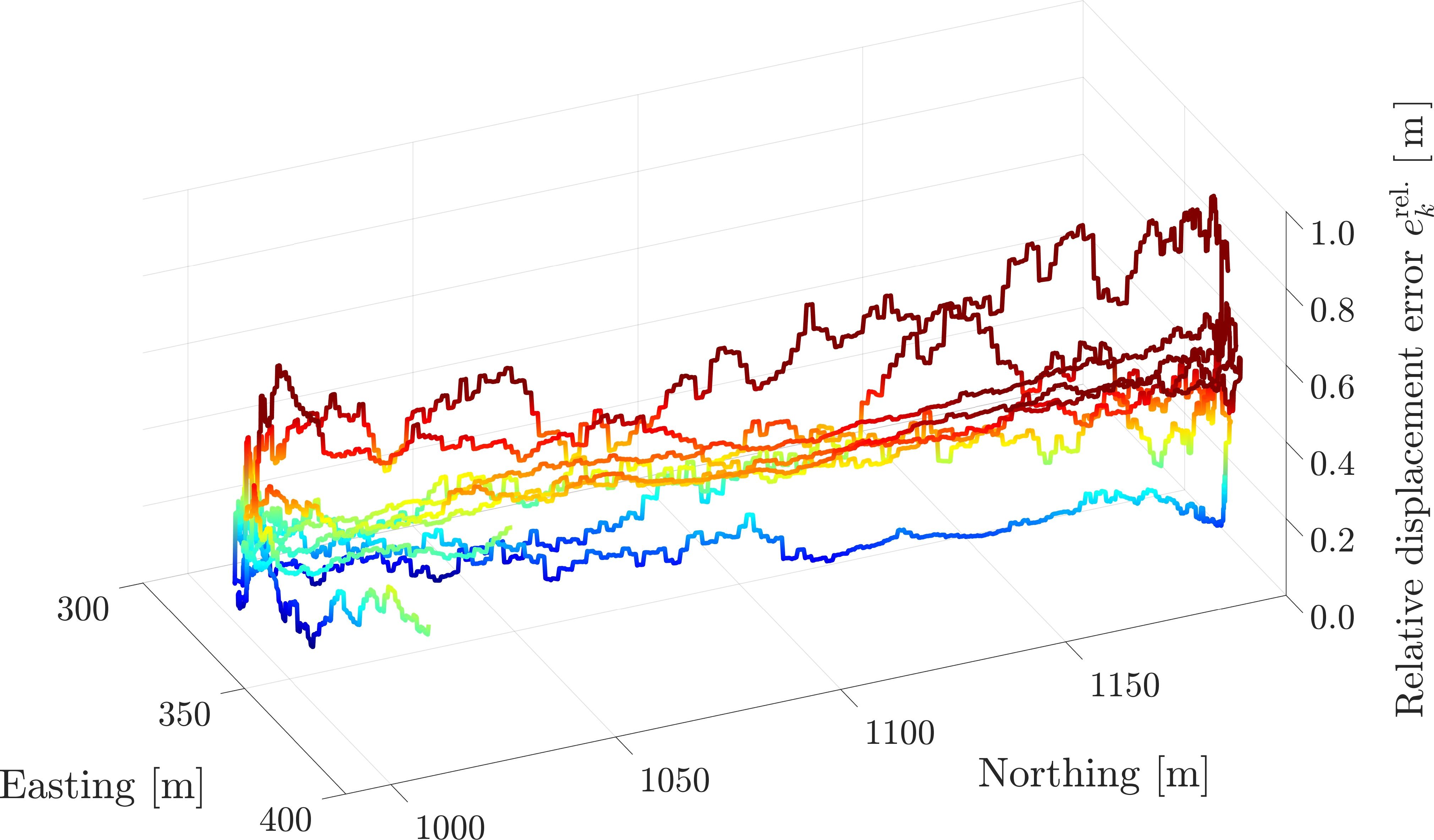
(b) INS isometric. Heatmap scale is identical to Figure 8(a).

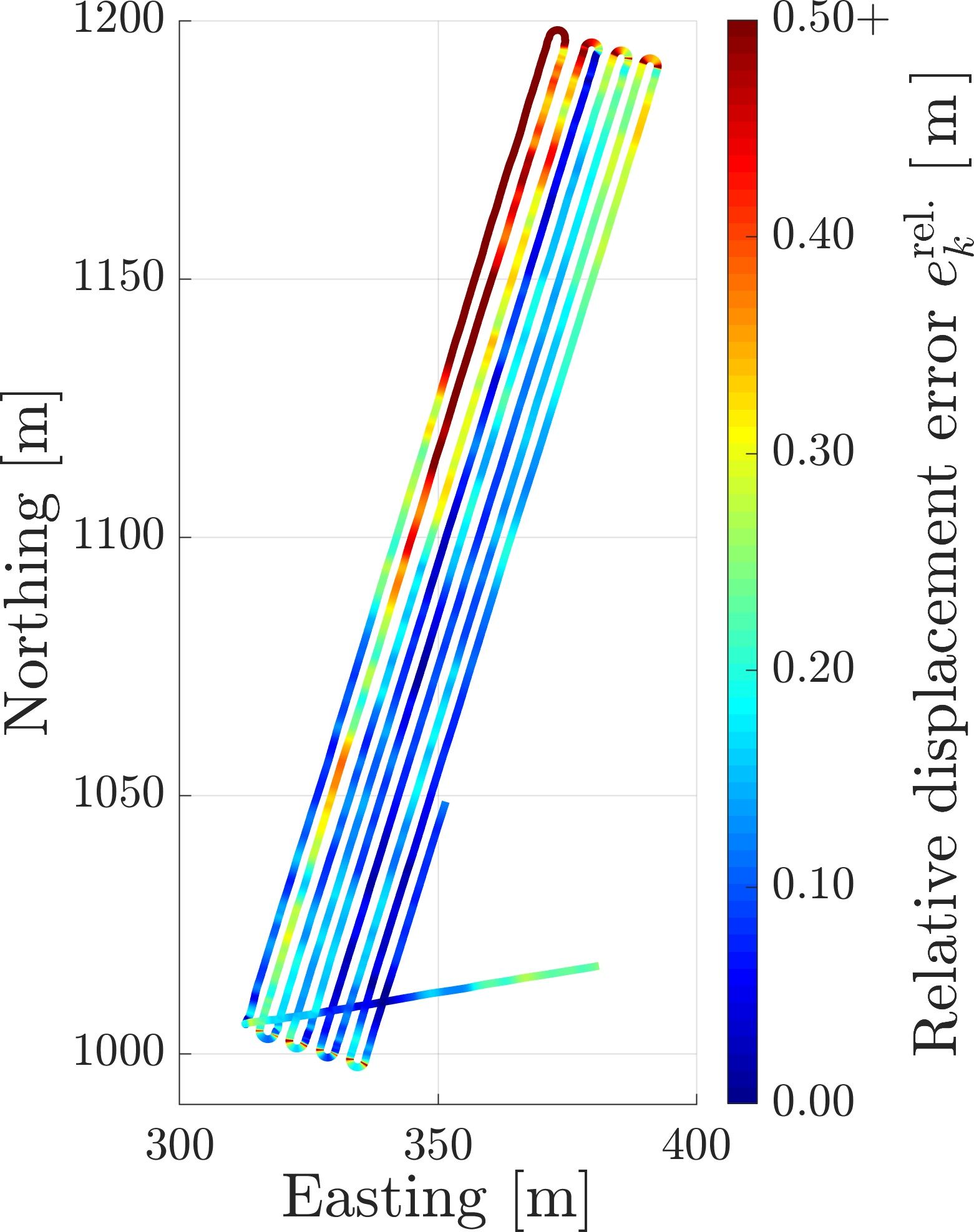
(c) INS+LC top

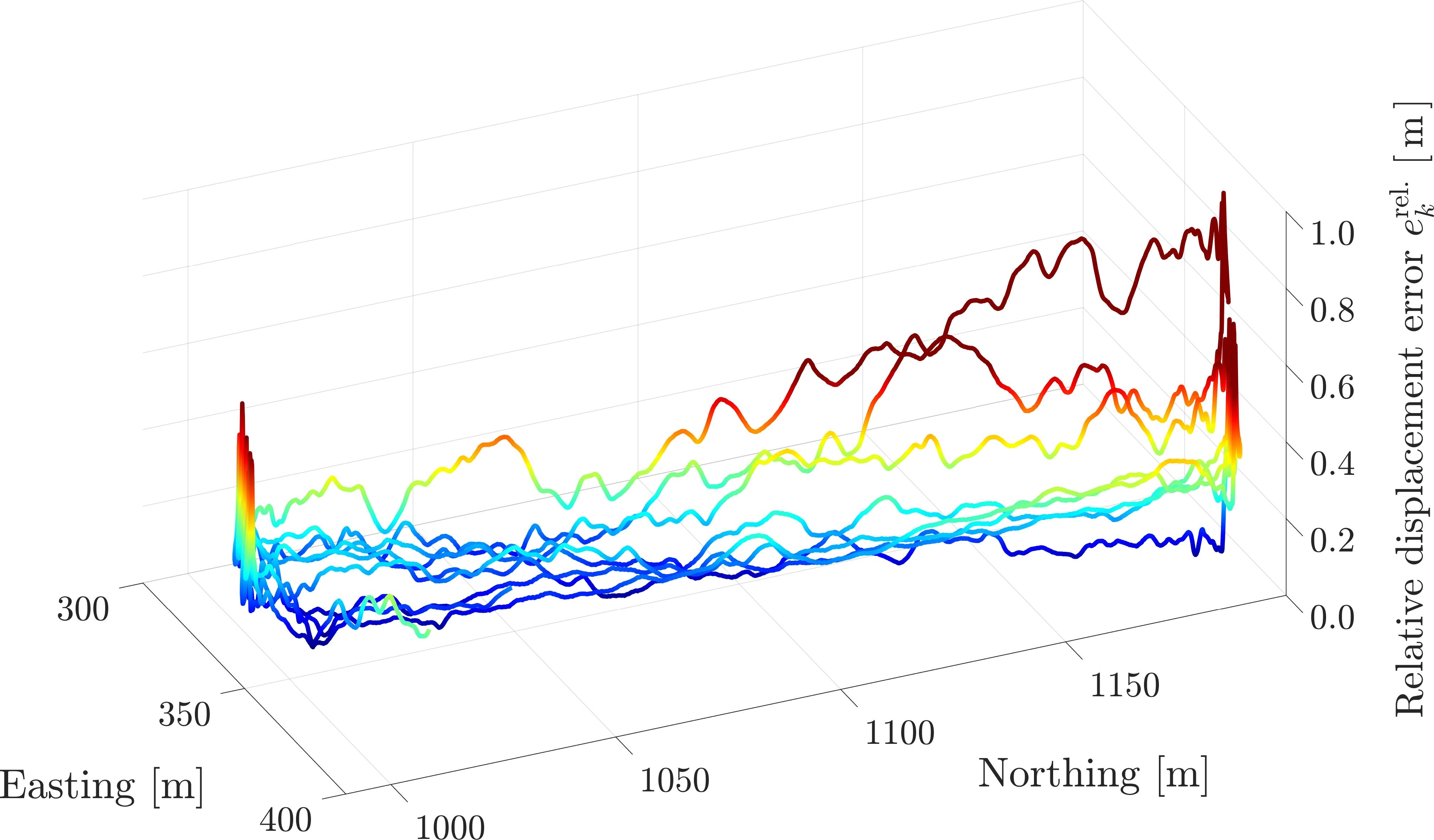
(d) INS+LC isometric. Heatmap scale is identical to Figure 8(c).

Figure 8: Heatmaps representing the relative displacement error for the INS and INS+LC trajectories. The left column shows a top view, while the right column shows an isometric view to illustrate the smoothing effects of the WNOA terms. Note the series of spikes at the far ends of Figure 8(d), where the vehicle completes low-radius turns to initiate the next survey pass.

Simulated output from a DVL-INS and a corresponding ground-truth trajectory were provided by industry collaborator Sonardyne. The DVL-INS output contains latitude and longitude, depth, and roll-pitch-yaw estimates for a simulated AUV deployment. At each time step, marginal variance estimates are available for the depth and heading states, and a joint covariance estimate is available for planar position in the local geodetic frame. $30\text{\,}\mathrm{min}$ of DVL-INS output data is available at a frequency of $5\text{\,}\mathrm{Hz}$. Note that the DVL-INS output has been heavily degraded by Sonardyne to better assess the ability of loop closures to mitigate navigation drift and does not reflect the performance of Sonardyne commercial products.

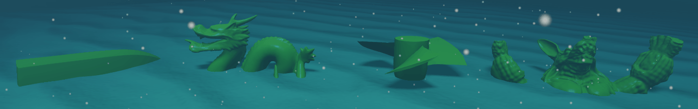
(a) An underwater scene generated in the Stonefish AUV simulator [62]. From left to right: boat hull, dragon, propeller, and armadillo. The hull and propellor are available in Stonefish, while the dragon and armadillo are from the Stanford 3D Scanning Repository [63].

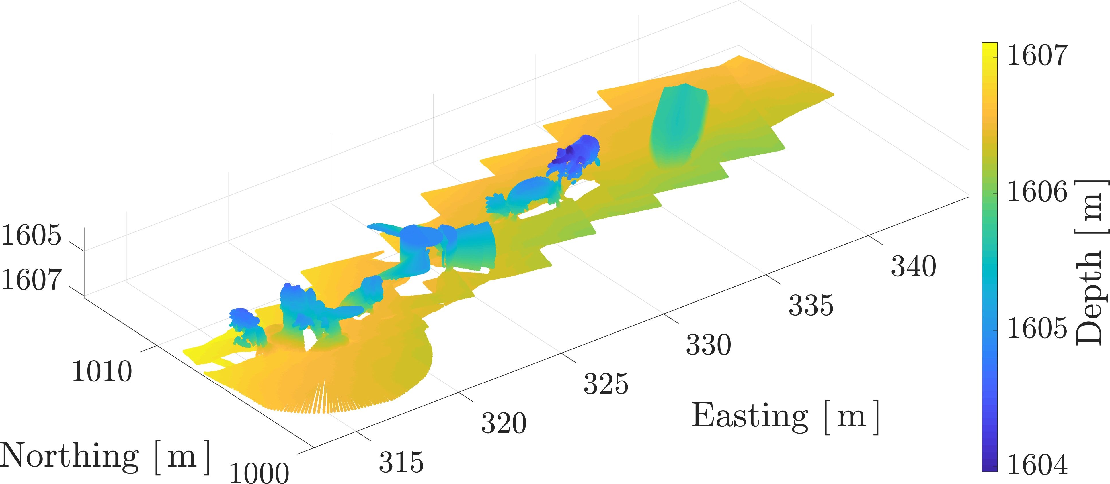
(b) Prior elevation (INS)

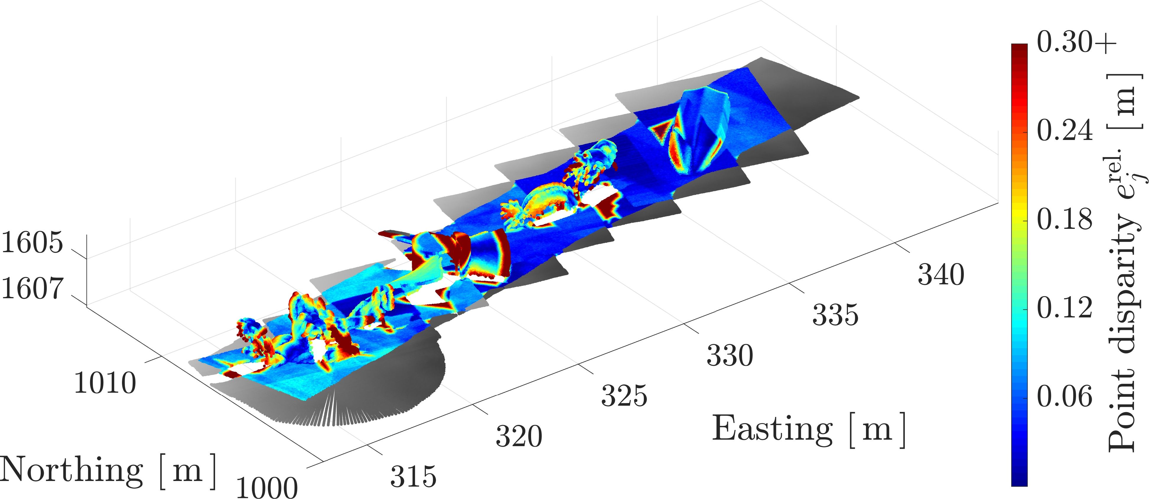
(c) Prior disparity (INS)

(d) Posterior elevation (INS+LC)

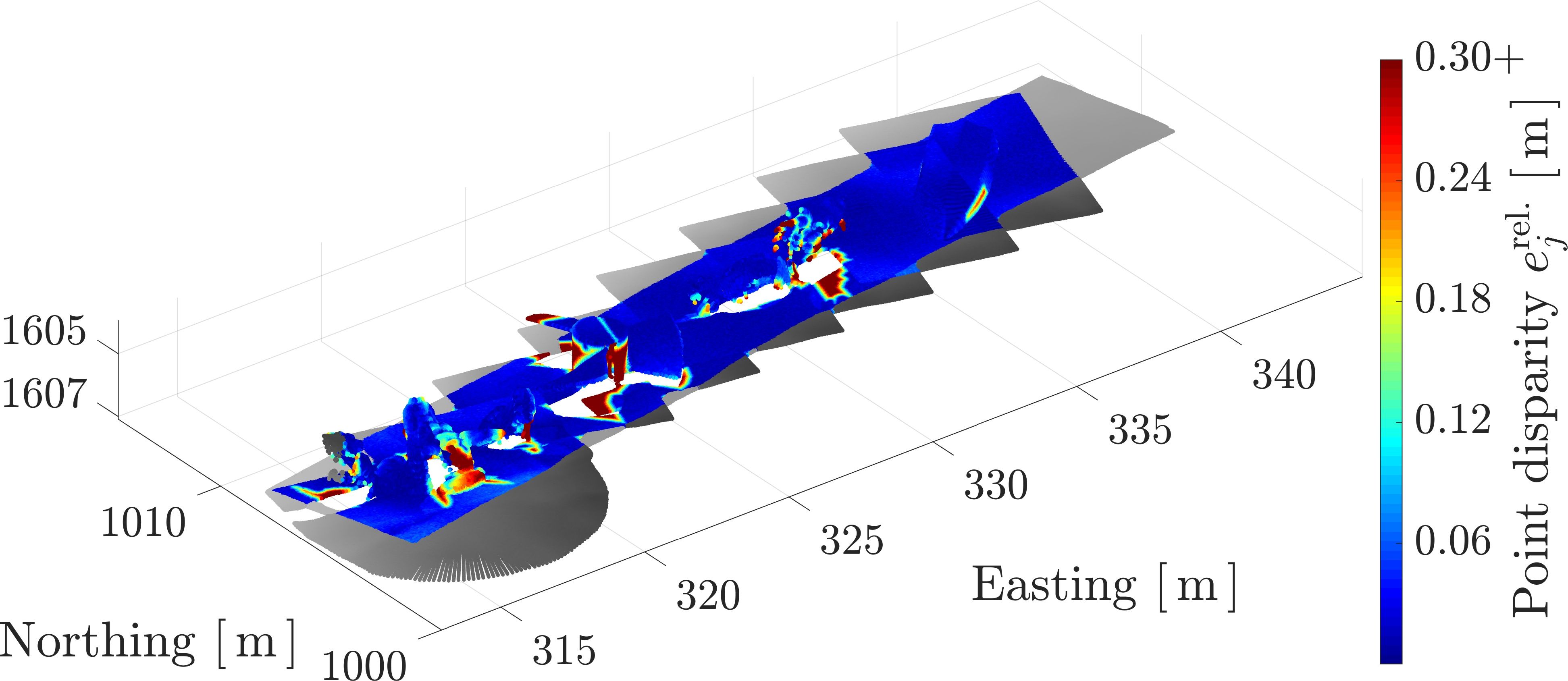
(e) Posterior disparity (INS+LC)

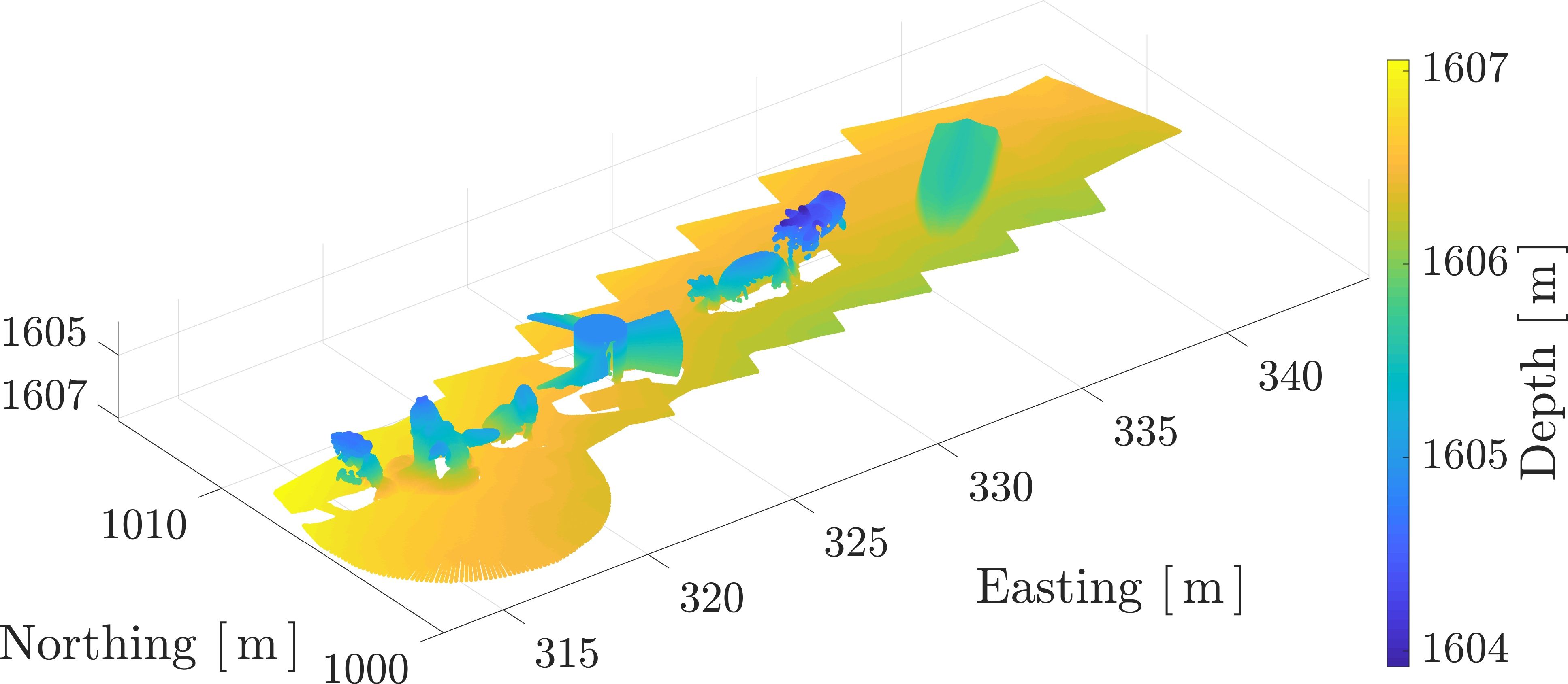
(f) Ground-truth elevation (INS+GPS)

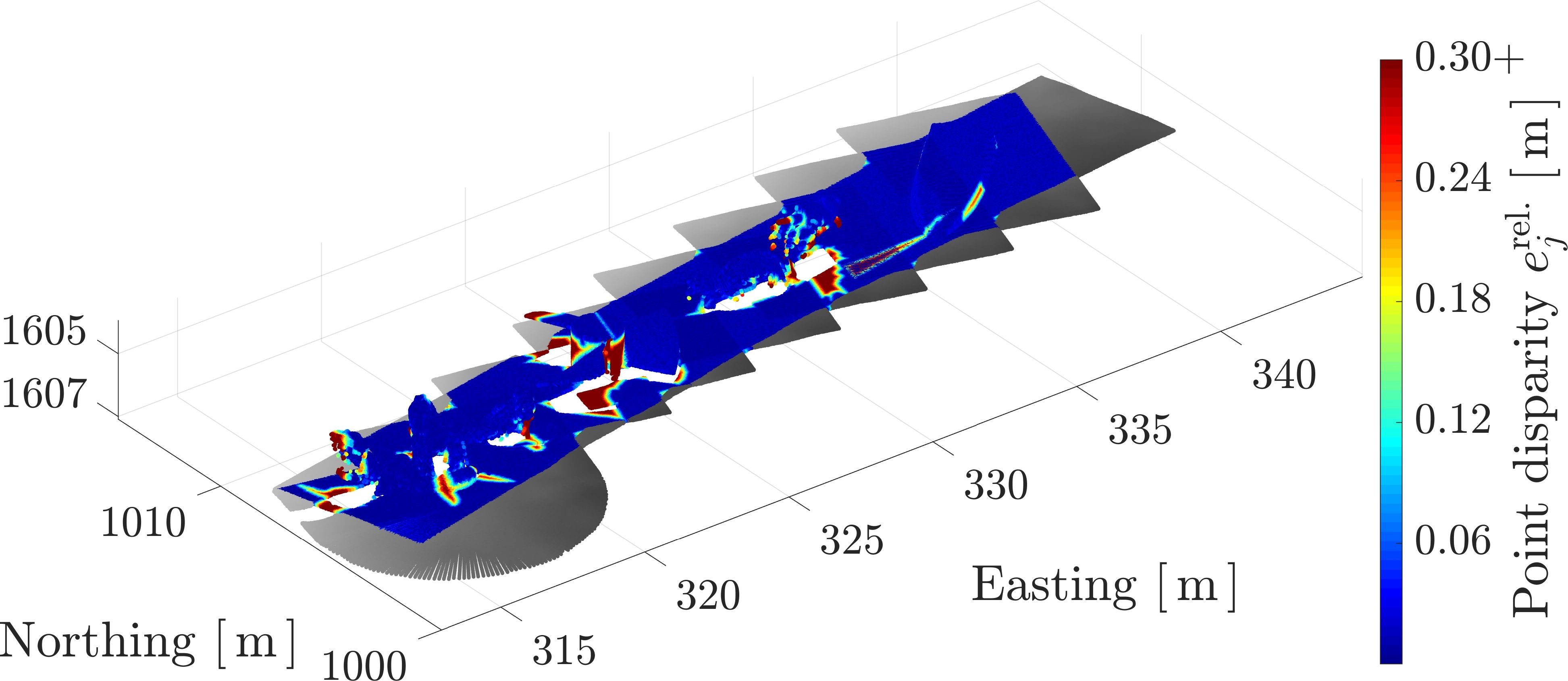
(g) Ground-truth disparity (INS+GPS)

Figure 9: Scanning a 3D scene in the Stonefish AUV simulator [62] to evaluate the quality of the point cloud map. The four models in Figure 9(a) are positioned along the tie-line near the loop-closure locations, and are scanned multiple times as the AUV completes the trajectory. Errors in the trajectory estimate are easily seen in the point disparity maps in the right column. Note the areas of high point disparity in the ground-truth map Figure 9(g) are due to occlusion of the range-bearing scanner. Scanning the 3D models at different orientations produces different occlusion patterns, leading to non-overlapping areas of the map. This in turn leads to large nearest-neighbour distances to points in other scans, and thus a high point disparity error.

The ground-truth trajectory is shown in Figure 7, where the vehicle starts with a single tie-line followed by multiple planar “lawnmower” passes over a large inspection area. Loop closures occur at the eight intersections between the lawnmower passes and the tie-line. The prior “INS” estimate is then conditioned on the loop-closure measurements using the methodology from Section III to produce a posterior “INS+LC” trajectory estimate. Both estimates are then compared to the ground-truth solution (“GT”) using the metrics from Section IV-A. The application and propagation of loop-closure measurements within the WNOA framework is expected to produce a more accurate navigation solution with a correspondingly more self-consistent point cloud map.

To illustrate the improvements in accuracy and the smoothing effect from the WNOA terms, Figure 8 displays the relative displacement error $e^{\textrm{rel.}}_{k}$ as a “heatmap” for the prior INS and posterior INS+LC trajectories. From Figure 8(a) it is clear that the prior estimate is not accurate, with relative displacement errors exceeding $0.5\text{\,}\mathrm{m}$ for much of the trajectory. Incorporating loop-closure measurements improves the accuracy of the trajectory estimate, as demonstrated by the cooler colours throughout the heatmap in Figure 8(c). The improvement is particularly noticeable around the tie-line at the bottom of Figure 8(c), however for many of the passes the effects extend hundreds of meters beyond the loop-closure location, increasing the accuracy across the entire inspection area. Relative displacement errors of $0.5\text{\,}\mathrm{m}$ may seem inconsequential at this scale, but may prove critical for certain subsea activities such as jumper pipe installation.

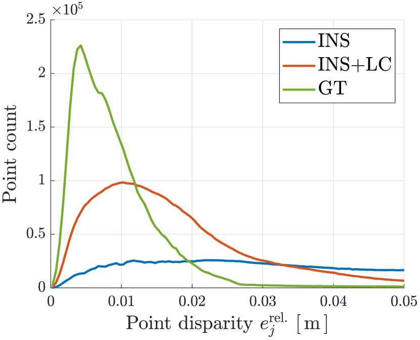
(a) Empirical probability density functions (EPDF)

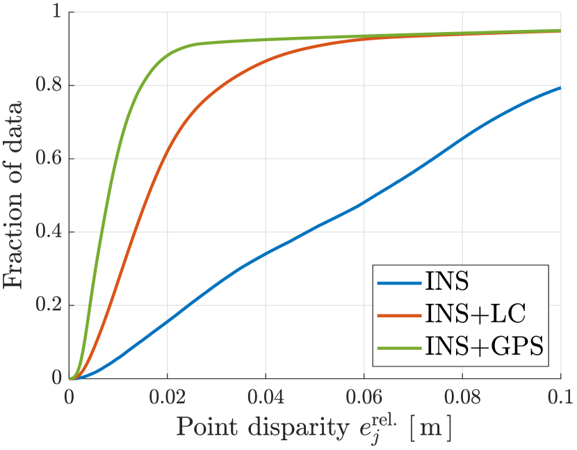
(b) Empirical cumulative distribution functions (ECDF)

Figure 10: Distributions on the point disparity error for each of the three navigation solutions for the simulated AUV area inspection dataset. The INS+LC solution greatly improves on the prior INS solution, virtually eliminating errors beyond $6\text{\,}\mathrm{cm}$. The relatively uniform error distribution for the INS solution is visible in the heatmap of Figure 9(c).

The smoothing effects from the WNOA motion prior are visible in Figures 8(b) and 8(d), which are, respectively, isometric views of Figures 8(a) and 8(c). Here, the relative displacement error is represented both by the heatmap and the plot elevation. The prior INS estimate shows visible step changes in the relative displacement error, which are characteristic of the correction step of a filter and likely represent the effects of DVL measurements within the DVL-INS estimation algorithm. In contrast, the posterior INS+LC estimate has been visibly smoothed due to the presence of the WNOA error terms. Trajectory smoothing is important in this context, as the point cloud map is generated by registering individual laser profiles to the trajectory estimate. A trajectory with step changes will produce a map with step changes, which will surely impact front-end activities such as feature detection and point cloud alignment. A smooth, self-consistent map is also visually appealing, and will improve the accuracy of subsea metrology.

Note the series of “spikes” in the relative displacement error of Figure 8(d), corresponding to the posterior trajectory estimate. These spikes occur at the beginning and end of each low-radius turn, suggesting that the smoothing effect of the WNOA terms may be erasing trajectory information in high-curvature regions. A geometry-based trajectory upsampling approach, for example based on scale-invariant density [64], is expected to resolve this, and will be explored as part of future work.

To evaluate the effects of the optimization on map quality, an underwater scene was constructed and scanned using the open-source AUV simulator Stonefish [62]. Raw laser profiles were collected along the ground-truth trajectory, and were then registered to the INS and INS+LC trajectories to produce, respectively, the prior and posterior point cloud maps. The 3D scene in Stonefish, as well as the resulting elevation and point disparity maps, are shown throughout Figure 9.

TABLE IV: Critical values from the ECDF of Figure 10(b). For example, for the INS solution, $95.45\text{\,}\mathrm{\char 37\relax}$ ($2\sigma$) of point disparity errors are below $23.39\text{\,}\mathrm{cm}$. Occluded areas in the simulated point cloud scan are responsible for the large errors at the upper ends of the ECDF distributions.

Solution	$50\text{\,}\mathrm{\char 37\relax}$	$1\sigma$	$2\sigma$	$3\sigma$
INS	$6.23\text{\,}\mathrm{cm}$	$8.32\text{\,}\mathrm{cm}$	$23.39\text{\,}\mathrm{cm}$	$56.15\text{\,}\mathrm{cm}$
INS+LC	$1.61\text{\,}\mathrm{cm}$	$2.27\text{\,}\mathrm{cm}$	$11.60\text{\,}\mathrm{cm}$	$44.70\text{\,}\mathrm{cm}$
INS+GPS	$0.81\text{\,}\mathrm{cm}$	$1.13\text{\,}\mathrm{cm}$	$11.48\text{\,}\mathrm{cm}$	$45.64\text{\,}\mathrm{cm}$

Compared to the ground-truth disparity map Figure 9(g), the prior map Figure 9(c) shows high point disparity errors throughout, indicating a self-inconsistent map. In contrast, the disparity errors are largely resolved by the INS+LC solution, which incorporates both loop-closure measurements and smoothing into the INS estimate. The improvements are quantified in Figure 10 by plotting an empirical probability density function (EPDF) and an empirical cumulative distribution function (ECDF) of the disparity error for each of the three solutions. For a quantitative comparison, Table IV lists critical values drawn from the ECDF curves. The INS+LC solution improves on the INS solution by producing a larger fraction of points with a lower point disparity error. This is especially evident in Figure 10(b), where the INS+LC solution converges to the GT solution around $6\text{\,}\mathrm{cm}$. Assuming the remaining $5\text{\,}\mathrm{\char 37\relax}$ of errors lie in occluded regions, as explained in the caption of Figure 9, the INS+LC solution has effectively eliminated point disparity errors beyond $6\text{\,}\mathrm{cm}$. In contrast, $20\text{\,}\mathrm{\char 37\relax}$ of disparity errors from the prior INS solution exceed $10\text{\,}\mathrm{cm}$. “Double-vision” effects of this magnitude arising from poor scan alignment are sure to complicate inspection and metrology tasks, even within the small domain of this simulation. Following the methodology from Section III, the INS+LC solution has produced a smooth, crisp, self-consistent point cloud map from which relative distance measurements may accurately be drawn.

IV-D Field Results: Wiarton Shipwreck

A field trial was conducted with Voyis Imaging Inc. in Colpoy’s Bay, Wiarton, Ontario, Canada. The bay is shallow and contains multiple shipwrecks and other manmade structures, making it an ideal test location for Voyis’s surface vessel. The full test trajectory is shown in blue in Figure 11(a). A section of the trajectory, highlighted in green in the northeast corner of Figure 11(a), makes eight passes over a small shipwreck. Figure 11(b) shows this section in detail, and Figure 11(c) shows the main shipwreck structure segmented from the lakebed. This section of the trajectory, which is approximately $580\text{\,}\mathrm{m}$ long and took $10.5\text{\,}\mathrm{min}$ to complete, is the focus of the field results.

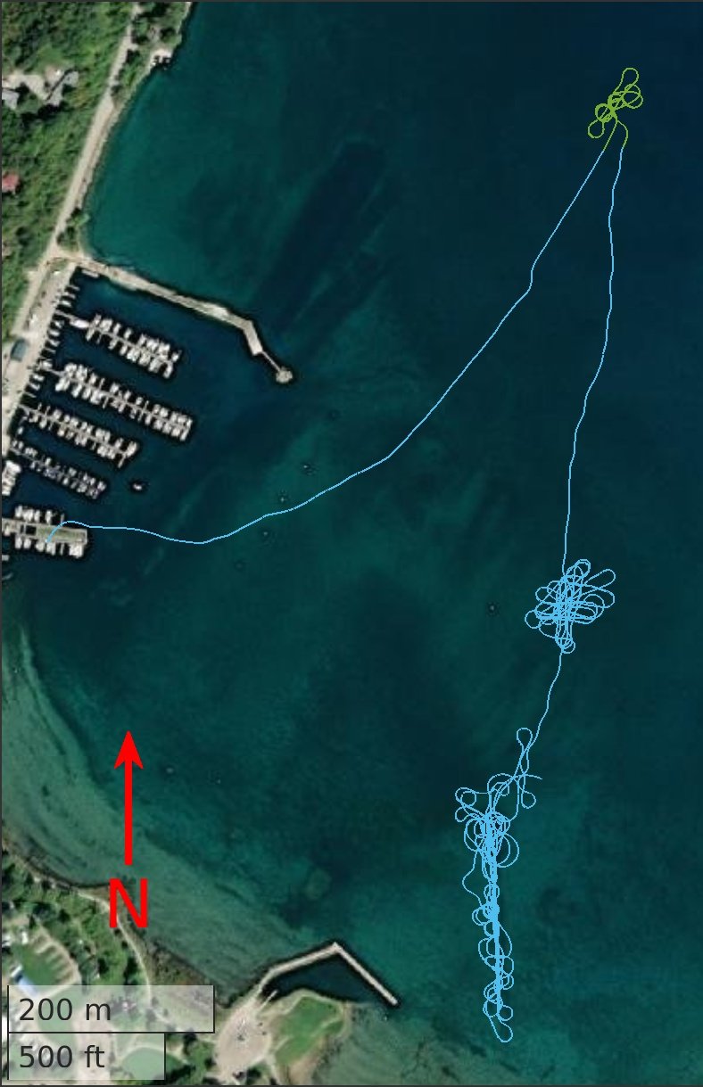
(a) The test trajectory, with shipwreck section in green in northeast corner.

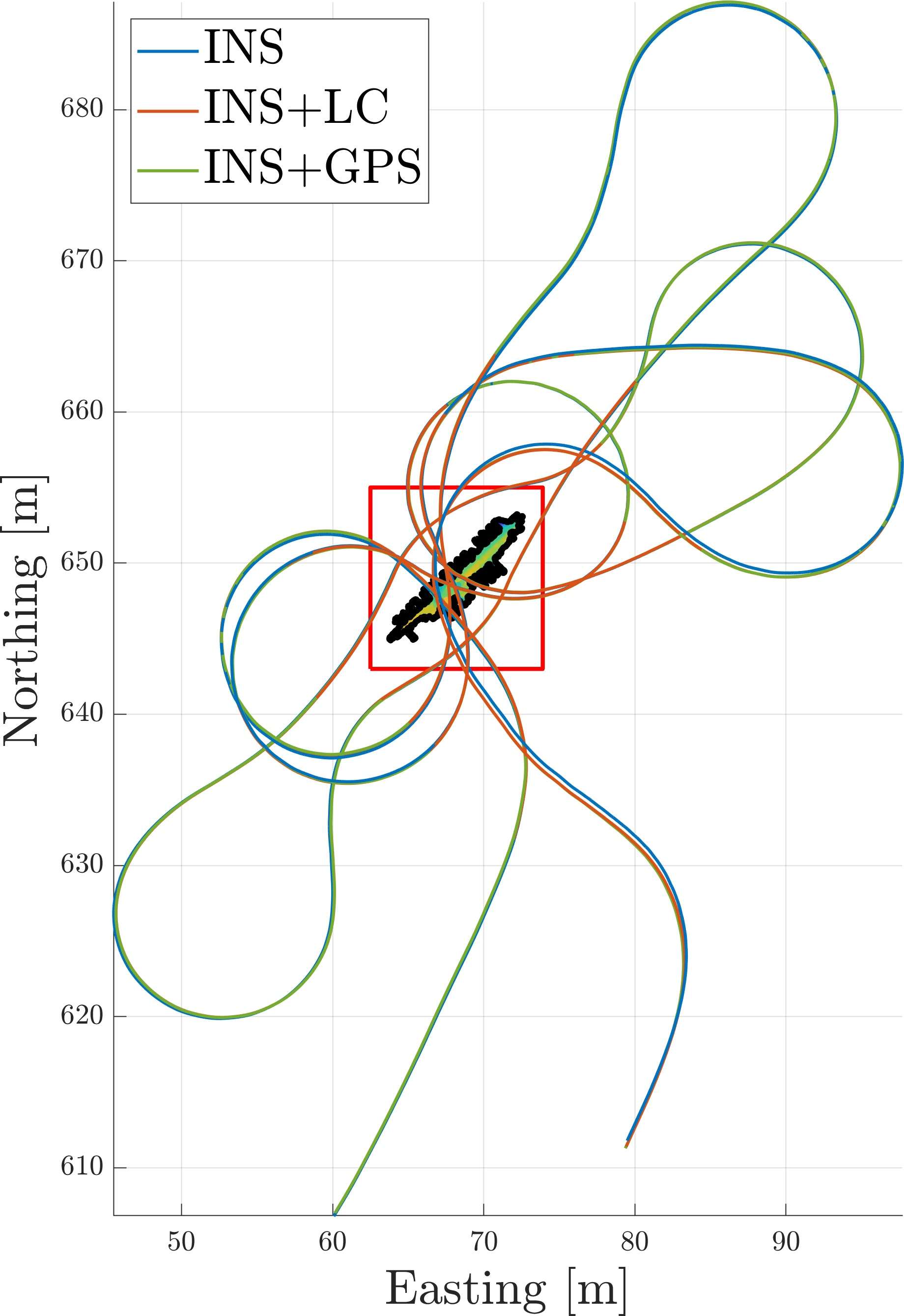
(b) Shipwreck section, with different trajectory estimates and shipwreck area.

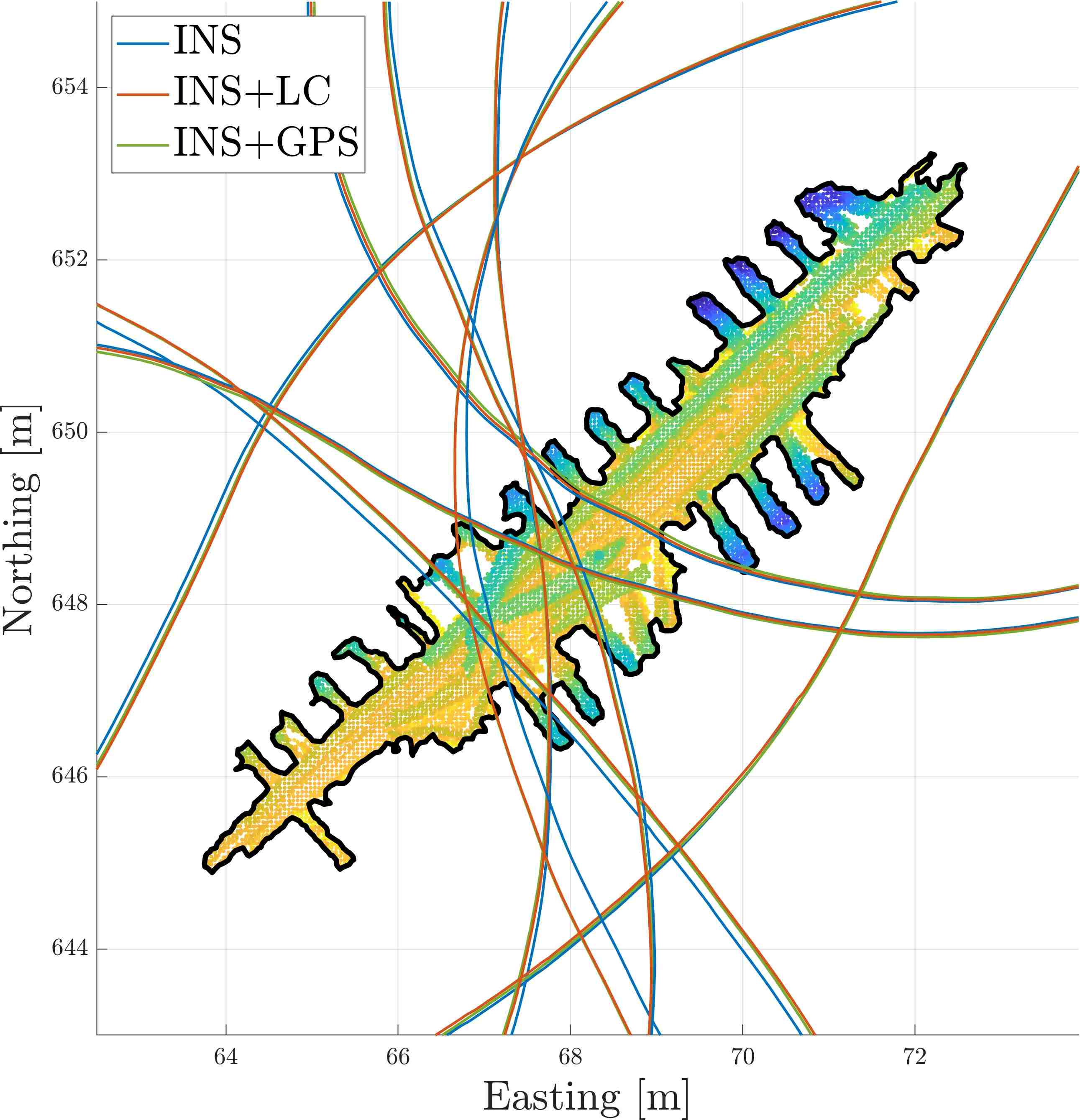
(c) The boxed region from Figure 11(b), showing the outline of the main shipwreck structure.

Figure 11: Field deployment in Colpoy’s Bay, Wiarton, Ontario, Canada. The full trajectory is shown in Figure 11(a). The shipwreck section, shown in green in northeast corner of Figure 11(a), is $0.58\text{\,}\mathrm{km}$ long and took approximately $10.5\text{\,}\mathrm{min}$ to complete. The trajectory makes eight passes over the shipwreck area. The different navigation solutions are summarized in Table V.

The surface vessel was equipped with a Sonardyne SPRINT-Nav 500 DVL-aided INS, a u-blox ZED-F9P high precision GNSS module equipped with a u-blox ANN-MB series high precision multi-band antenna, and a Voyis Insight Pro underwater laser scanner. GNSS data were post-processed using the Canadian Spacial Reference System Precise Point Positioning (CSRS-PPP) application [65], which in a recent study was found to be capable of measuring 2D position with a precision of $2\text{\,}\mathrm{cm}$ ($1\sigma$) [66].

Three navigation solutions were generated from these data. The first solution is a dead-reckoned DVL-INS trajectory (“INS”), where the positioning precision of the SPRINT-Nav 500 has been manually degraded by Sonardyne from the nominal value of $0.02\text{\,}\mathrm{\char 37\relax}$ of distance traveled (CEP50) [52, Sec. 4.9.1.2][13]. The DVL-INS output is available at $10\text{\,}\mathrm{Hz}$. Note that this solution is representative of the state-of-the-art for high-grade commercial systems, and will be used to benchmark the proposed methodology. The second solution, referred to as “INS+LC,” applies the methodology of Section III to incorporate loop-closure measurements into the dead-reckoned DVL-INS estimate. Batch processing was performed offline in MATLAB, taking approximately $90\text{\,}\mathrm{s}$ to converge on a laptop with an E3-1505M v5 CPU and $16\text{\,}\mathrm{GB}$ of RAM. It is important to note that this solution is produced using the DVL-INS state estimate, without access to the raw DVL-INS sensor measurements. The third solution fuses the DVL-INS output with the GNSS data to form a ground-truth estimate (“INS+GPS”). The three navigation solutions are summarized in Table V, and the trajectory estimates are overlaid on the shipwreck area in Figures 11(b) and 11(c).

TABLE V: Understanding the different navigation solutions for the Wiarton shipwreck field dataset.

Solution	Description
INS	Dead-reckoned DVL-INS solution, with position precision manually degraded by Sonardyne.
INS+LC	The dead-reckoned DVL-INS trajectory estimate conditioned on loop-closure measurements. Raw sensor measurements from the DVL-INS are inaccessible, and GNSS data is not used as part of this solution.
INS+GPS	DVL-aided INS solution with GNSS correction.

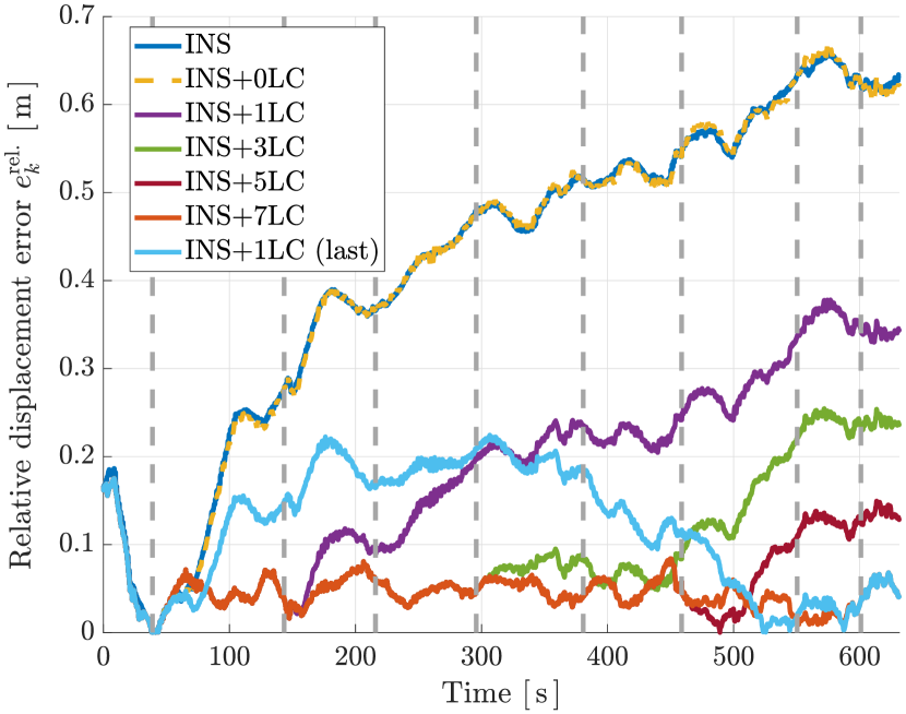
Figure 12: Relative displacement errors for trajectory estimates incorporating an increasing number of loop closures. Loop-closure locations are marked as vertical dashed lines, and “INS+XLC” indicates the first X loop closures were used in generating the estimate. Incorporating loop closures bounds navigation drift over time. For numerical results, see Table VI.

TABLE VII: Summary statistics on relative pose errors (69) computed for the Wiarton field trial. Relative attitude errors $|\delta\phi^{\textrm{rel.}}_{i}|$ have been broken down by component, while the rightmost column gives statistics on the norm of the relative body-centric position error. Cumulative statistics for each error are reported in the format $50\text{\,}\mathrm{\char 37\relax}$ $\cdot$ $75\text{\,}\mathrm{\char 37\relax}$ $\cdot$ $90\text{\,}\mathrm{\char 37\relax}$.

Solution	$|\delta\phi^{\textrm{rel.}}_{1}|\,\left[\deg\right]$	$|\delta\phi^{\textrm{rel.}}_{2}|\,\left[\deg\right]$	$|\delta\phi^{\textrm{rel.}}_{3}|\,\left[\deg\right]$	$\|\delta\bm{\rho}^{\textrm{rel.}}\|\,\left[\operatorname{m}\right]$
INS	$1.110-3$ $\cdot$ $1.910-3$ $\cdot$ $2.510-3$	$1.510-3$ $\cdot$ $2.410-3$ $\cdot$ $3.510-3$	$1.510-2$ $\cdot$ $1.910-2$ $\cdot$ $2.210-2$	$0.482$ $\cdot$ $0.562$ $\cdot$ $0.630$
INS+LC	$1.110-1$ $\cdot$ $2.710-1$ $\cdot$ $5.310-1$	$1.210-1$ $\cdot$ $3.810-1$ $\cdot$ $5.710-1$	$1.510-2$ $\cdot$ $2.010-2$ $\cdot$ $2.210-2$	$0.077$ $\cdot$ $0.096$ $\cdot$ $0.108$

Incorporating loop-closure measurements produces a more accurate trajectory estimate, as measured by the relative displacement error (70). Figure 12 shows the relative displacement error, measured against the ground-truth INS+GPS estimate, for the dead-reckoned INS trajectory and the INS+LC trajectory with an increasing number of loop closures. The loop-closure locations are marked with vertical dashed lines, with the first observation of the shipwreck occurring approximately $40\text{\,}\mathrm{s}$ in to the trajectory. The relative displacement drift in the INS trajectory estimate increases without bound, while the maximum displacement error decreases monotonically as more loop-closure measurements are applied. Even a single loop-closure measurement at the end of the trajectory is effective in bounding the relative displacement drift over time, as demonstrated by the cyan line in Figure 12. From Table VI, which summarizes the maximum error and final error as a percent of distance traveled for the different solutions, the final drift error for the “INS+1LC (last)” solution is $6.8210-3\text{\,}\mathrm{\char 37\relax}$ of distance traveled. This particular solution suggests an order of magnitude improvement over state-of-the-art DVL-INS systems [13]. Importantly, the dashed yellow “INS+0LC” curve in Figure 12 indicates that the posterior solution does not deviate far from the prior DVL-INS solution when loop-closure measurements are absent. This suggests that the proposed methodology may still be used to smooth the DVL-INS solution in the absence of loop-closure measurements, without sacrificing solution accuracy. For example, the maximum position drift error for the “INS-0LC” solution tabulated in Table VI is only $9\text{\,}\mathrm{mm}$

TABLE VI: Summary of drift errors from Figure 12, with values drawn after the first shipwreck observation at $40\text{\,}\mathrm{s}$.

Solution	Max drift [$\text{\,}\mathrm{m}$]	Final %DT
INS	0.658	$10.9810-2\text{\,}$
INS+0LC	0.667	$10.8210-2\text{\,}$
INS+1LC	0.378	$5.9910-2\text{\,}$
INS+3LC	0.255	$4.1210-2\text{\,}$
INS+5LC	0.150	$2.2510-2\text{\,}$
INS+7LC	0.084	$6.8310-3\text{\,}$
INS+1LC (last)	0.224	$6.8210-3\text{\,}$

greater than the maximum drift observed in the “INS” solution. However, note the proposed methodology is intended to be used in a targeted fashion in situations where at least one loop-closure measurement is available.

In addition to the relative displacement errors summarized in Figure 12, relative pose errors (69) are computed across the trajectory for the prior “INS” and posterior “INS+LC” solutions, with summary statistics given in Table VII. Relative attitude errors in Table VII are decomposed into body-centric roll, pitch, and yaw, while the rightmost column gives statistics on the Euclidean norm of the body-centric relative position errors. Interestingly, the proposed methodology has produced an increase in the relative body-centric pitch and roll errors, from median values of $1.110-3\text{\,}\deg$ and $1.510-5\text{\,}\deg$, respectively, to $1.110-1\text{\,}\deg$ and $1.210-1\text{\,}\deg$, respectively. Relative body-centric yaw errors remain largely unchanged by the proposed methodology, while trends in the relative body-centric position error generally follow the trend of the relative displacement error plotted in Figure 12. For example, $90\text{\,}\mathrm{\char 37\relax}$ of body-centric position errors for the prior “INS” solution fall below $0.630\text{\,}\mathrm{m}$, while the corresponding value for the posterior “INS+LC” solution is $0.108\text{\,}\mathrm{m}$.

An increase in roll and pitch errors may seem concerning, however the posterior errors remain low and bounded. Such errors were likely introduced in this field trial through a combination of small angular errors in the INS-laser extrinsics estimate and the relatively weak pitch and roll prior used in the optimization (see (38) and the value of hyperparameter $\sigma_{\textrm{rp}}$ in Table III). The more important result is that relative body-centric position errors remain low and bounded when multiple loop-closure measurements are present.

Barring measurement outliers, finding that loop closures improve trajectory accuracy is not particularly surprising in a conventional state estimation context. However, these results have been achieved following the methodology of Section III, without access to raw sensor measurements, a vehicle process model, exteroceptive sensor models, or sensor noise and bias specifications. The loop-closure corrections have instead been smoothly integrated into the DVL-INS estimate using the factor graph illustrated in Figure 6, improving the accuracy of the trajectory estimate.

Incorporating loop-closure measurements produces a more self-consistent point cloud map, as measured by the point disparity error (71). Figure 13 shows the point disparity in the shipwreck area as a heatmap, for each of the three navigation solutions. The disparity is computed for each of the eight passes over the wreck, and is the Euclidean distance from each point in one pass to its nearest neighbour in the remaining seven passes. A highly accurate trajectory estimate is expected to produce a tightly overlapping, crisp point cloud map from the composite scans, with a low point disparity error.

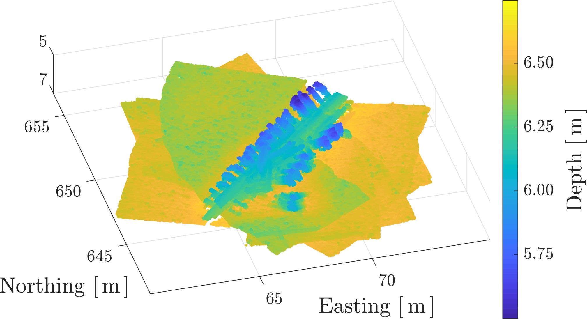
(a) Prior elevation (INS)

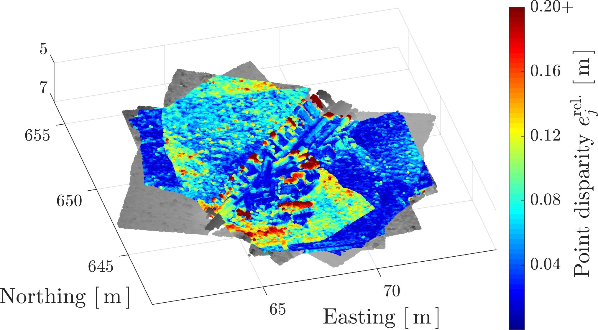
(b) Prior disparity (INS)

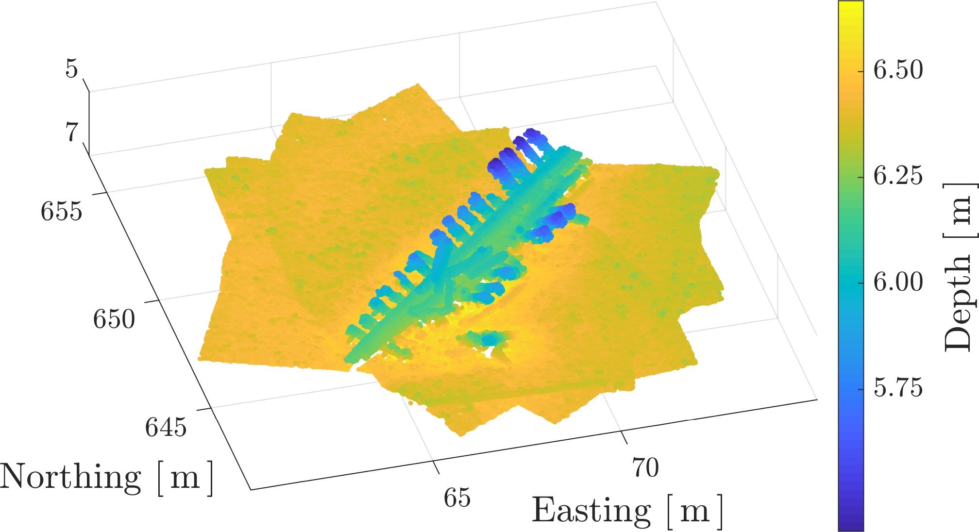
(c) Posterior elevation (INS+LC)

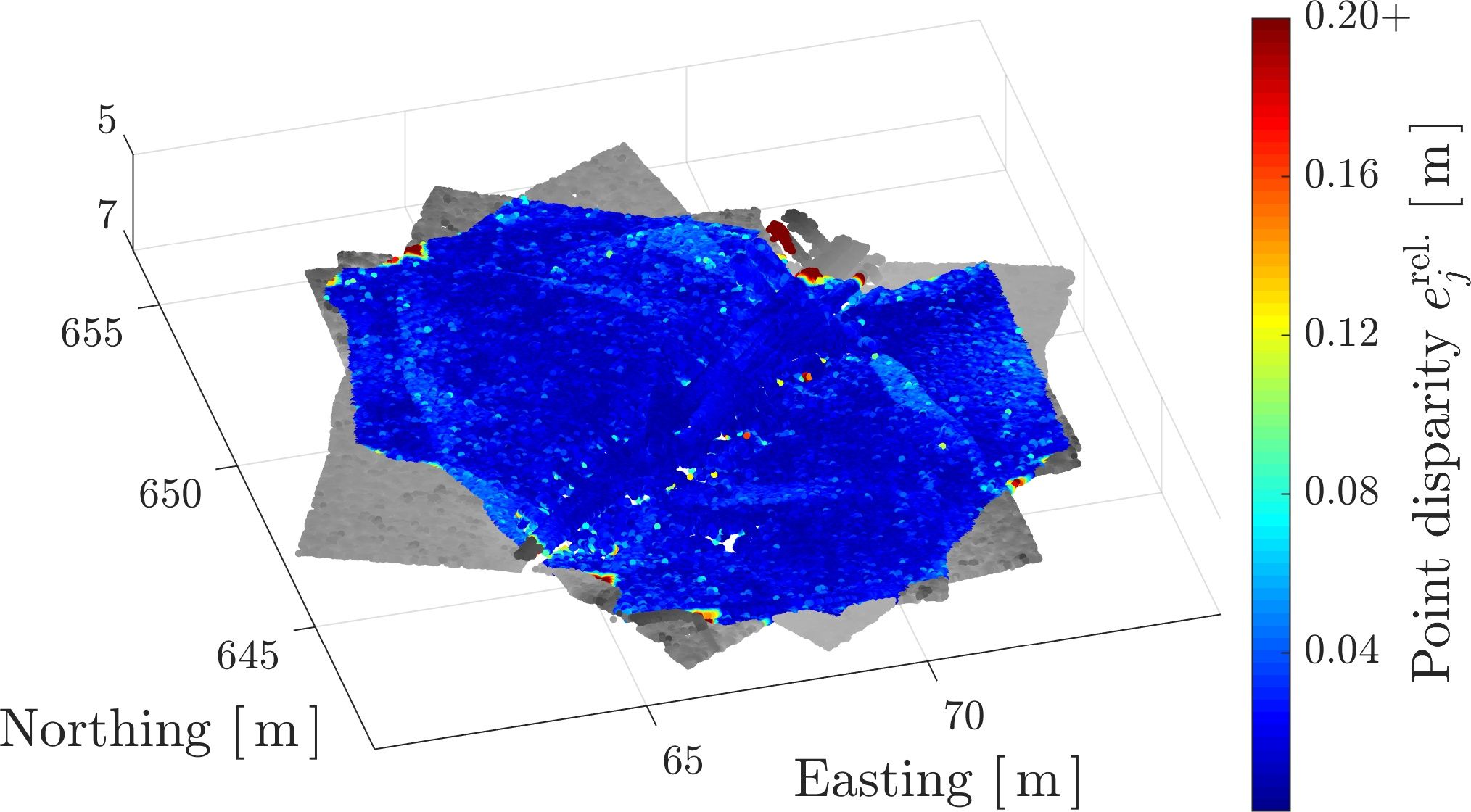
(d) Posterior disparity (INS+LC)

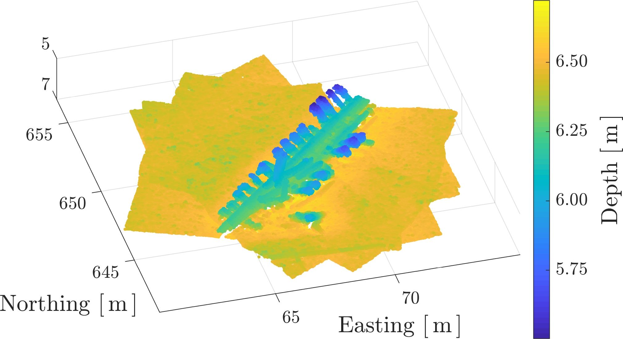
(e) Ground-truth elevation (INS+GPS)

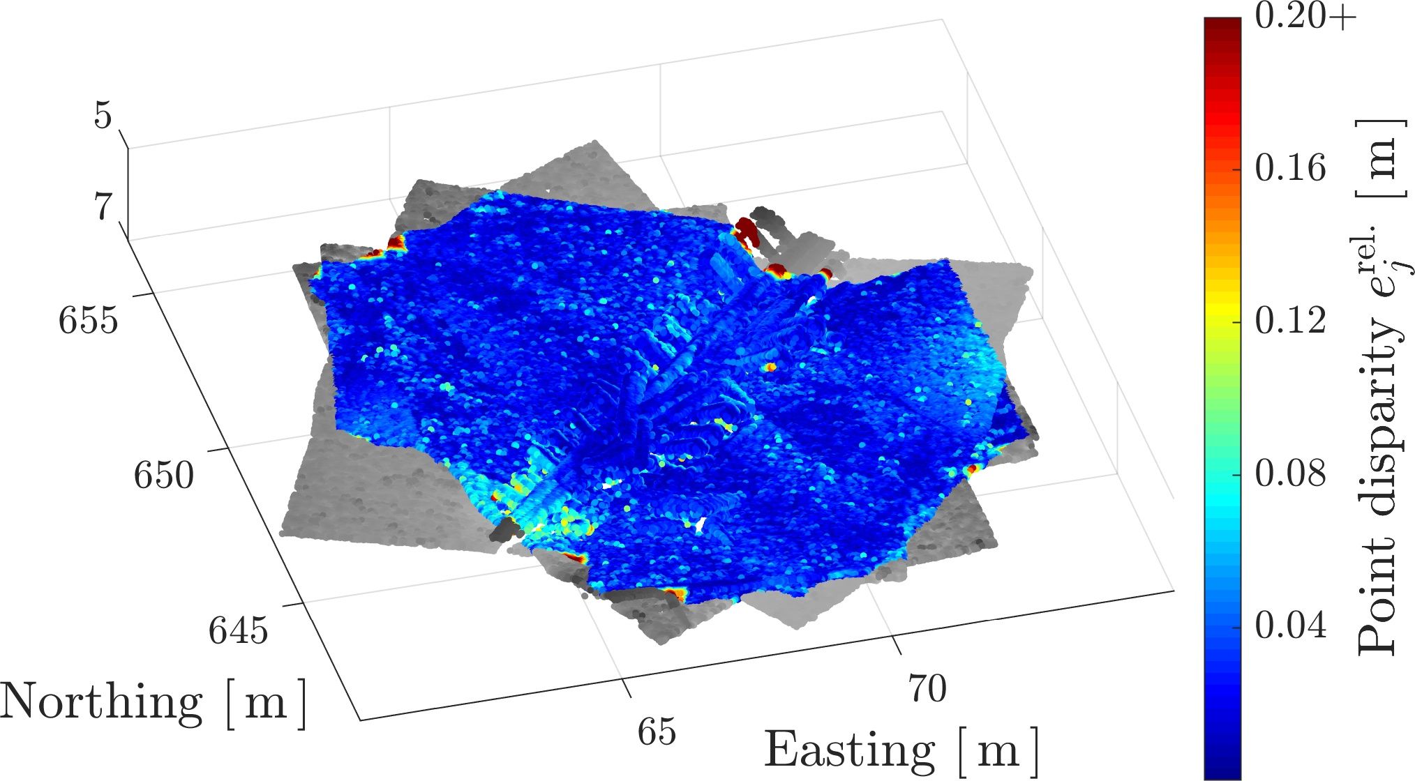
(f) Ground-truth disparity (INS+GPS)

Figure 13: Visualizing the point disparity error in the shipwreck area for the three navigation solutions. Left column: colour map indicates depth, and has been included for context. Right column: colour map indicates point disparity.

From a qualitative evaluation of Figure 13(b), the dead-reckoned INS trajectory estimate has clearly produced a self-inconsistent point cloud map. Areas around the ribs of the shipwreck have point disparity errors of around $20\text{\,}\mathrm{cm}$, while one of the passes shows relatively large errors on the seabed owing to drift in the depth dimension. In contrast, both the posterior and the ground-truth estimates have produced highly self-consistent maps, with low point disparity errors throughout.

Interestingly, the INS+LC solution produces a point cloud map that is more self-consistent than the ground-truth estimate. This is difficult to judge qualitatively from Figure 13, however Figure 14 shows the EPDF and ECDF of the disparity error for each of the three navigation solutions. Critical values from the ECDF are tabulated in Table VIII. In Figure 14(a), the INS+LC curve peaks to the left of the INS+GPS curve, indicating a lower overall point disparity error and thus a more self-consistent point cloud map [5]. This is likely due to a combination of small estimation errors in the ground-truth solution and small errors in the scanner extrinsics estimate $\mbf{T}^{sz}_{b\ell}$ from (24). It should therefore come as no surprise that the INS+LC solution delivers a more self-consistent map, as the point disparity error is precisely what is minimized during point cloud alignment (26). For additional images of the shipwreck area generated using the prior and posterior navigation solutions, see Appendix B.

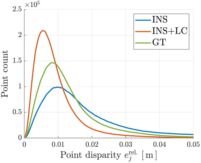
(a) Empirical probability density functions (EPDF)

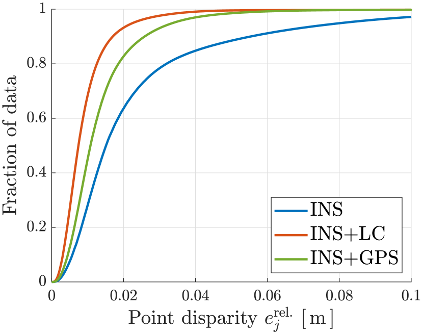
(b) Empirical cumulative distribution functions (ECDF)

Figure 14: Distributions on the point disparity error for each of the three navigation solutions for the Wiarton shipwreck field dataset. The posterior INS+LC solution produces a more self-consistent point cloud map than the ground-truth INS+GPS solution, likely owing to a combination of residual navigation and extrinsics errors. Critical values from the ECDF are summarized in Table VIII.

TABLE VIII: Critical values from the ECDF of Figure 14(b). For example, for the INS solution, $95.45\text{\,}\mathrm{\char 37\relax}$ ($2\sigma$) of point disparity errors are below $8.51\text{\,}\mathrm{cm}$. Note the improvement in the INS+LC solution over the INS+GPS solution.

Solution	$50\text{\,}\mathrm{\char 37\relax}$	$1\sigma$	$2\sigma$	$3\sigma$
INS	$1.51\text{\,}\mathrm{cm}$	$2.23\text{\,}\mathrm{cm}$	$8.42\text{\,}\mathrm{cm}$	$18.11\text{\,}\mathrm{cm}$
INS+LC	$0.75\text{\,}\mathrm{cm}$	$1.00\text{\,}\mathrm{cm}$	$2.35\text{\,}\mathrm{cm}$	$7.23\text{\,}\mathrm{cm}$
INS+GPS	$1.08\text{\,}\mathrm{cm}$	$1.45\text{\,}\mathrm{cm}$	$3.49\text{\,}\mathrm{cm}$	$8.63\text{\,}\mathrm{cm}$

Again, this improvement in map self-consistency has been achieved without access to the standard ingredients available in typical state estimation problems. Visualizing the point cloud map and the resulting disparity errors is a straightforward way to verify that the loop-closure measurements have been successfully applied, and that the updates have been smoothly propagated throughout the trajectory.

Compared to the GPS-aided solution, the improvement in map self-consistency that comes from leveraging loop-closure measurements may appear modest. However, an improvement on the order of centimeters may be consequential for certain subsea inspection tasks, such as measuring deformation in manmade structures. In this respect, the methodology of Section III offers a valuable addition to inspection and metrology work. This is especially true for dead-reckoned solutions, but remains true even when localizing measurements are available, for example LBL, USBL, or GPS measurements.

A Monte Carlo experiment was conducted on the Wiarton field dataset to test the effectiveness of the loop-closure measurement outlier rejection method discussed in Section III-B3. To run the experiment, between one and five of the seven loop-closure measurements were randomly replaced by randomly generated measurements. Thirty Monte Carlo trials were conducted for each outlier corruption level, for a total of 150 trials. The number of trials at each corruption level was chosen to provide a representative statistical sample. Additionally, the experimental results obtained using 30 trials per corruption level were very similar to results obtained when using 20 and 25 trials per level.

The outlier measurements were generated to mimic the outliers experimentally observed in the detector/descriptor study in Section III-A2. Outlier position measurements were uniformly sampled so that ${\|\mbf{r}^{\textrm{xy}}\|\leq$5\text{\,}\mathrm{m}$}$ and ${r^{\textrm{z}}\in\left[\left[$-0.5\text{\,}\mathrm{m}$,$0.5\text{\,}\mathrm{m}$\right]\cup\left[$13.5\text{\,}\mathrm{m}$,$14.5\text{\,}\mathrm{m}$\right]\right]}$, with ${\mbf{r}^{\textrm{out}}=\begin{bmatrix}(\mbf{r}^{\textrm{xy}})^{\mathsf{T}}&r^{\textrm{z}}\end{bmatrix}^{\mathsf{T}}}$. This reflects both the planar search bound used to detect loop-closure candidates (27) as well as the range “flipping” effect discussed in Section III-A2. Outlier attitude measurements were uniformly sampled according to ${\phi^{\textrm{out}}_{j}\in(-\pi,\pi]\ $\text{\,}\mathrm{rad}$,j=1,2,3}$. An outlier measurement $\bm{\Xi}^{\textrm{out}}_{\ell_{1}\ell_{2}}$ is then generated according

$$\bm{\Xi}^{\textrm{out}}_{\ell_{1}\ell_{2}}=\begin{bmatrix}\mbf{C}^{\textrm{out}}(\bm{\phi}^{\textrm{out}})&\mbf{r}^{\textrm{out}}\\ \mbf{0}&1\end{bmatrix}.$$ (73)

Results from this experiment are summarized throughout Figure 15. All 150 Monte Carlo trials are plotted in Figure 15(a), along with the ground-truth “INS+GPS” trajectory and the prior “INS” trajectory estimate. No visible navigation failures are seen in Figure 15(a), implying the adaptive robust cost function is effective in rejecting false loop-closure measurements. A zoom of the shipwreck region in Figure 15(b) shows the Monte Carlo trajectory samples gracefully decaying from the ground-truth solution to the prior estimate as more outliers are included. This behaviour is also seen in the relative displacement error plot of Figure 15(c), where the mean relative $(x,y)$ navigation drift (70) is plotted for each outlier corruption level. The trend of higher outlier rates producing larger relative drift values is reminiscent of the ablation study summarized in Figure 12, in which loop-closure measurements are simply removed from the solution. This provides sound evidence that the proposed outlier rejection algorithm is successful in identifying and removing false loop-closure measurements.

Finally, the grey patch in Figure 15(c) shows the worst-case relative displacement error at each time step across all 150 Monte Carlo trials. Compared to the prior “INS” estimate (blue curve), it is clear that, for this dataset, the proposed methodology delivers worst-case posterior estimates that are, at any given time, no worse than the prior estimate, even in instances with extreme outlier rates.

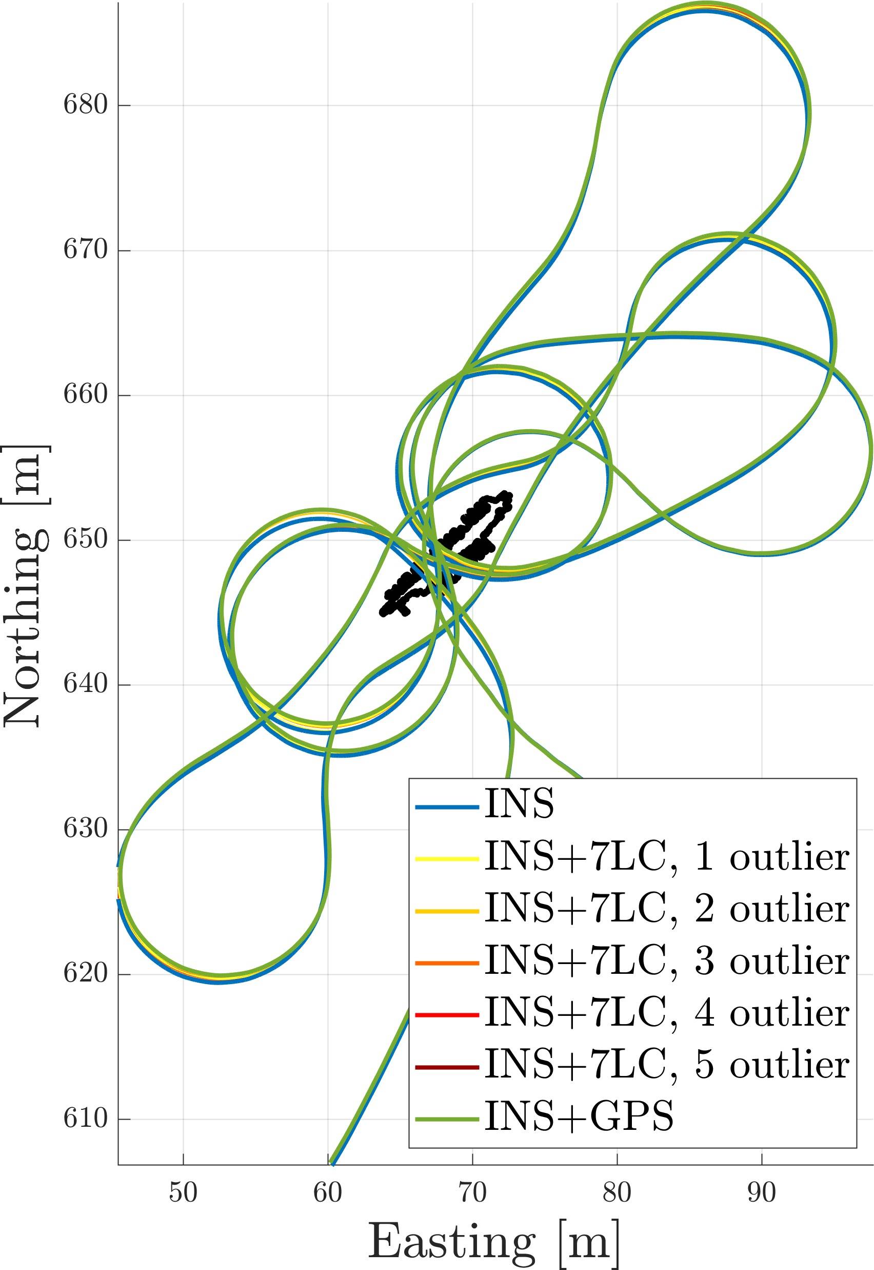
(a) 150 Monte Carlo trajectories

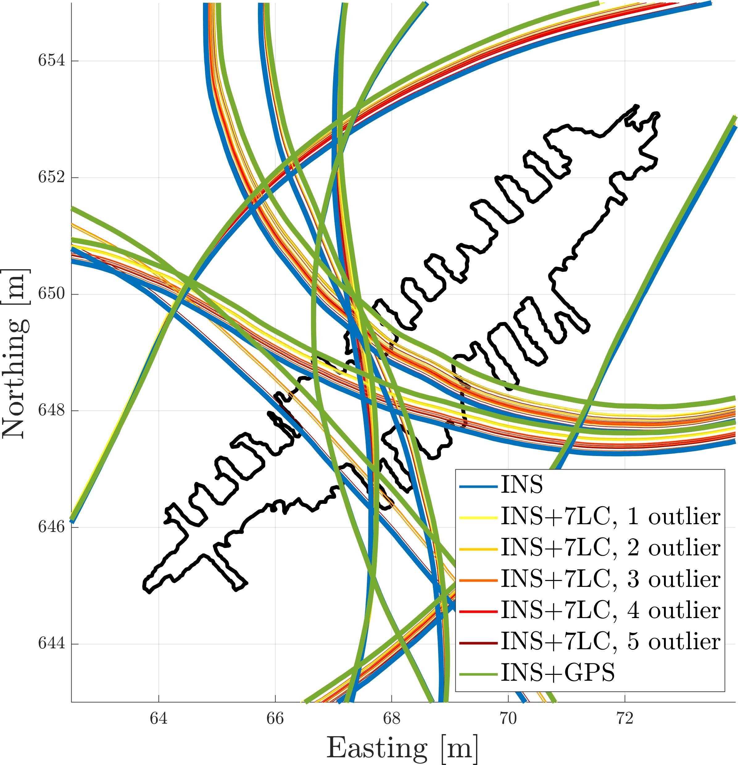
(b) Shipwreck section

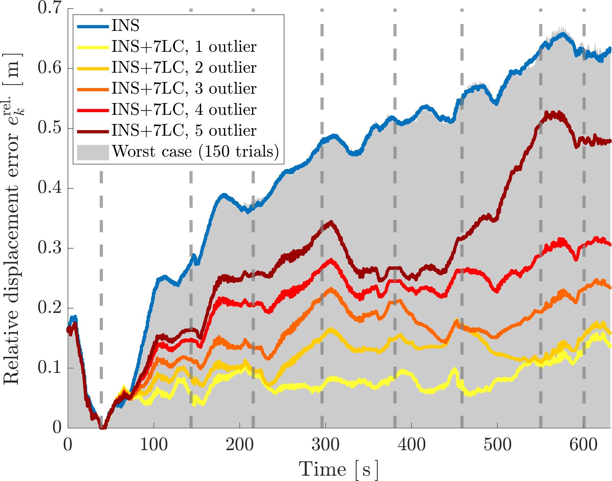
(c) Mean navigation drift by outlier corruption level

Figure 15: Trajectory estimates and associated relative drift errors (70) for 150 Monte Carlo trials. For each trial, between 1 and 5 of the seven loop-closure measurements are replaced by outlier measurements (73), with 30 trials conducted per outlier corruption level. The outlier rejection method discussed in Section III-B3 is effective in rejecting false loop-closure measurements, with no failures visible in Figure 15(a). The zoom in Figure 15(b) show a graceful decay from the ground-truth “INS+GPS trajectory” to the prior “INS” estimate as more outlier measurements are added. This is confirmed by the relative displacement error plot in Figure 15(c), which simply follows the trend of measurement removal first seen in the ablation study of Figure 12. The worst-case position drift at each time step measured across all 150 trials is shown as a grey patch in Figure 15(c). When compared against the relative displacement error from the prior “INS” estimate (blue line), the proposed methodology is seen to produce estimates that are, at any given time, no worse than the prior estimate, even in instances with extreme outlier rates.

V Conclusion

This works presents a novel and comprehensive method for systematically conditioning the output of a COTS DVL-INS navigation system on loop-closure measurements for the purpose of improving the self-consistency [4, 59] of the resulting bathymetric map. The method relies on a combination of relative pose and white-noise-on-acceleration [28] error terms to smoothly integrate the measurements in a batch state estimation framework.

The first contribution of this work is the development of a robust front-end algorithm for computing high-precision loop-closure measurements from 3D scans of challenging underwater environments. Second, loop-closure measurements are cleanly incorporated into an existing state estimate via a factor graph optimization framework, without access to raw sensor measurements, sensor models, or other information typically required in conventional state estimation problems.

The effectiveness of the proposed method was demonstrated for both simulated and field datasets using loop-closure measurements from an underwater laser scanner. The same simple hyperparameter structure was used for both studies, with good results. For the field results, conditioning the dead-reckoned DVL-INS estimate on loop-closure measurements produced a markedly more self-consistent point cloud map of an underwater shipwreck. Incorporating all seven loop-closure measurements resulted in a maximum relative position drift of $8.4\text{\,}\mathrm{cm}$ over a $576\text{\,}\mathrm{m}$ trajectory, with a final position error of $6.8310-3\text{\,}\mathrm{\char 37\relax}$ of distance traveled. This represents an order of magnitude improvement over unaided commercial DVL-INS systems. Additionally, the proposed methodolgy was demonstrated to be robust to false loop-closure measurements.

Future work will primarily focus on hyperparameter training through an expectation-maximization framework, for example [67] and [68]. The algorithm will be tested over longer trajectories with more varied terrain, including open seabed [8]. Finally, future work may also incorporate image information, in the form of conventional image descriptors and textured point cloud maps.

Thomas Hitchcox received his B.Eng. and M.Eng. degrees in mechanical engineering in 2015 and 2018, respectively, from McGill University, Montreal, QC, Canada. He is currently a Ph.D. Candidate with the Department of Mechanical Engineering at McGill. His research interests include state estimation, computer vision, and robust algorithms for point cloud filtering and alignment.

James Richard Forbes James Richard Forbes received the B.A.Sc. degree in Mechanical Engineering (Honours, Co-op) from the University of Waterloo, Waterloo, ON, Canada in 2006, and the M.A.Sc. and Ph.D. degrees in Aerospace Science and Engineering from the University of Toronto Institute for Aerospace Studies (UTIAS), Toronto, ON, Canada in 2008 and 2011, respectively. James is currently an Associate Professor and William Dawson Scholar in the Department of Mechanical Engineering at McGill University, Montreal, QC, Canada. James is a Member of the Centre for Intelligent Machines (CIM), and a Member of the Group for Research in Decision Analysis (GERAD). James was awarded the McGill Association of Mechanical Engineers (MAME) Professor of the Year Award in 2016, the Engineering Class of 1944 Outstanding Teaching Award in 2018, and the Carrie M. Derick Award for Graduate Supervision and Teaching in 2020. The focus of James’ research is navigation, guidance, and control of robotic systems.

Appendix A Supporting Derivations

[labelprefix=A]

A-A Introduction

The purpose of this appendix is to derive in detail the prior, process, and loop closure Jacobians appearing in Section III-B2 of “Improving Self-Consistency in Underwater Mapping through Laser-Based Loop Closure.” Key identities from matrix Lie group theory are reviewed in Section A-B, and the white-noise-on-acceleration (WNOA) motion prior [28] is reviewed in Section A-C. Section A-D examines the WNOA error kinematics. Finally, the necessary Jacobians are derived in Section A-E. The intent of this appendix is to make these derivations accessible, with key steps and identities indicated throughout. For a more detailed treatment of matrix Lie group theory, please consult the references cited throughout, particularly [23] and [24].

A-B Preliminaries

A-B1 Matrix Lie groups

A matrix Lie group $G$ is a set of real, invertible ${n\times n}$ matrices that is closed under matrix multiplication. Associated with every matrix Lie group is a matrix Lie algebra $\mathfrak{g}$, defined as the tangent space at the group identity, ${\mathfrak{g}\triangleq T{1}G}$. The matrix Lie algebra is a vector space closed under the operation of the Lie bracket [26, Sec. 10.2.6]. It is often more convenient to work with isometric representations of matrix Lie algebra elements, namely ${\bm{\xi}\in\mathbb{R}^{d}}$, where ${\bm{\xi}^{\wedge}\in\mathfrak{g}}$.

A Lie group and its corresponding Lie algebra are related through the exponential map. For matrix Lie groups this is simply the matrix exponential [23, Sec. 7.1.3]. For ${\mbf{X}\in G}$, this leads to expressions of the form

$$\mbf{X}=\exp(\bm{\xi}^{\wedge}),$$ (A.1)

where $\bm{\xi}^{\wedge}$ is the representation of $\mbf{X}$ in $\mathfrak{g}$, and $\bm{\xi}$ is the representation of $\mbf{X}$ in $\mathbb{R}^{d}$. Finally, the matrix logarithm is used to move from the matrix Lie group to the matrix Lie algebra, as in

$$\bm{\xi}^{\wedge}=\log\left(\mbf{X}\right).$$ (A.2)

The relationship between a matrix Lie group, its associated matrix Lie algebra, and the isometric space $\mathbb{R}^{d}$, as well as several other quantities discussed throughout this document, is illustrated in Figure A.1, which is inspired by, but modified from, [Bourmaud2015a].

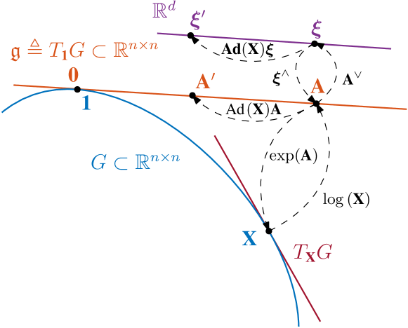
Figure A.1: Matrix Lie groups, modified from [Bourmaud2015a]. Mappings are shown between the matrix Lie group element $\mbf{X}$, its matrix Lie algebra representation ${\mbf{A}=\bm{\xi}^{\wedge}}$, and its $\mathbb{R}^{d}$ representation $\bm{\xi}$. Note the difference between the adjoint operator $\operatorname{Ad}(\cdot)$ and the adjoint matrix, $\operatorname{\mbf{Ad}}(\cdot)$, discussed in Section A-B4. All perturbations are modeled in the matrix Lie algebra $\mathfrak{g}$ (orange), defined as the tangent space at the group identity.

A-B2 Errors and perturbations on matrix Lie groups

There are four ways to define a matrix Lie group error [25]. These are summarized in Table A.1, along with their corresponding perturbation schemes. The error definition and perturbation scheme are linked. For example the selection of a left-invariant error definition necessitates the use of a left-invariant perturbation scheme. To see this, consider

$$\delta\mbf{X}= \ \mbf{X}^{-1}\bar{\mbf{X}},$$ (A.3a)

$$\exp(\delta\bm{\xi}^{\wedge})= \ \mbf{X}^{-1}\bar{\mbf{X}},$$

$$\mbf{X}\exp(\delta\bm{\xi}^{\wedge})= \ \mbf{X}\mbf{X}^{-1}\bar{\mbf{X}},$$

$$\mbf{X}= \ \bar{\mbf{X}}\exp(-\delta\bm{\xi}^{\wedge}),$$ (A.3b)

where (A.3a) is the left-invariant matrix Lie group error and (A.3b) is the left-invariant perturbation scheme. This work uses a left-invariant error definition.

TABLE A.1: Matrix Lie group error definitions and corresponding perturbation schemes.

Error definition	Matrix Lie group error	Perturbation scheme
Right invariant	$\delta\mbf{X}=\bar{\mbf{X}}\mbf{X}^{-1}$	$\mbf{X}=\exp(-\delta\bm{\xi}^{\wedge})\bar{\mbf{X}}$
Right perturbation	$\delta\mbf{X}=\mbf{X}\bar{\mbf{X}}^{-1}$	$\mbf{X}=\exp(\delta\bm{\xi}^{\wedge})\bar{\mbf{X}}\hphantom{-}$
Left invariant	$\delta\mbf{X}=\mbf{X}^{-1}\bar{\mbf{X}}$	$\mbf{X}=\bar{\mbf{X}}\exp(-\delta\bm{\xi}^{\wedge})$
Left perturbation	$\delta\mbf{X}=\bar{\mbf{X}}^{-1}\mbf{X}$	$\mbf{X}=\bar{\mbf{X}}\exp(\delta\bm{\xi}^{\wedge})\hphantom{-}$

A-B3 The Baker-Campbell-Hausdorff (BCH) equation

The BCH equation describes how to combine elements of the matrix Lie algebra [26, Sec. 10.2.7],

$$\mbf{c}^{\wedge}=\log\left(\exp(\mbf{a}^{\wedge})\exp(\mbf{b}^{\wedge})\right),\vspace{-3pt}$$ (A.4)

where ${\mbf{a}^{\wedge},\mbf{b}^{\wedge},\mbf{c}^{\wedge}\in\mathfrak{g}}$. Elements of $\mathfrak{g}$ are therefore correctly combined on the group $G$, through application of the exponential map. However, the following approximation,

$$\mbf{c}\approx\mbf{a}+\mbf{J}^{\textrm{r}}(\mbf{a})^{-1}\mbf{b},\vspace{-3pt}$$ (A.5)

is valid if $\mbf{b}$ is small [23, Sec. 7.1.5], where $\mbf{J}^{\textrm{r}}(\bm{\xi})$ is the right Jacobian of $G$. The following approximation,

$$\mbf{c}\approx\mbf{a}+\mbf{b},\vspace{-3pt}$$ (A.6)

is valid if both $\mbf{a}$ and $\mbf{b}$ are small. This leads to the following three useful identities related to the BCH equation,

$$\exp(\bm{\xi}^{\wedge})\exp(\delta\bm{\xi}^{\wedge})\approx \ \exp\big{(}(\bm{\xi}+\mbf{J}^{\textrm{r}}(\bm{\xi})^{-1}\delta\bm{\xi})^{\wedge}\big{)},$$ (A.7a)

$$\exp((\bm{\xi}+\delta\bm{\xi})^{\wedge})\approx \ \exp(\bm{\xi}^{\wedge})\exp\big{(}(\mbf{J}^{\textrm{r}}(\bm{\xi})\delta\bm{\xi})^{\wedge}\big{)},$$ (A.7b)

$$\exp(\delta\bm{\xi}^{\wedge}_{1})\exp(\delta\bm{\xi}^{\wedge}_{2})\approx \ \exp\left(\left(\delta\bm{\xi}_{1}+\delta\bm{\xi}_{2}\right)^{\wedge}\right).$$ (A.7c)

A-B4 The adjoint operator and the adjoint matrix

The adjoint operator maps the effects of perturbations about the group identity to other group elements. For ${\mbf{X}\in G}$ and ${\bm{\xi}^{\wedge}\in\mathfrak{g}}$, the adjoint operator $\operatorname{Ad}:\mathfrak{g}\to\mathfrak{g}$ is defined as [30, Sec. 2.5]

$$\operatorname{Ad}(\mbf{X})\bm{\xi}^{\wedge}\triangleq\mbf{X}\bm{\xi^{\wedge}}\mbf{X}^{-1}.$$ (A.8)

The adjoint matrix $\operatorname{\mbf{Ad}}:\mathbb{R}^{d}\to\mathbb{R}^{d}$ encodes the effects of the adjoint operator directly on $\mathbb{R}^{d}$ [24],

$$\operatorname{\mbf{Ad}}(\mbf{X})\bm{\xi}\triangleq\left(\mbf{X}\bm{\xi}^{\wedge}\mbf{X}^{-1}\right)^{\vee}.\vspace{-3pt}$$ (A.9)

The adjoint matrix may also be defined in terms of the left and right group Jacobians [23, Sec. 7.1.5],

$$\operatorname{\mbf{Ad}}(\mbf{X})\triangleq\mbf{J}^{\ell}(\bm{\xi})\mbf{J}^{\textrm{r}}(\bm{\xi})^{-1},$$ (A.10)

where ${\mbf{J}^{\ell}(\bm{\xi})=\mbf{J}^{\textrm{r}}(-\bm{\xi})}$. Finally, the adjoint matrix exists in the matrix Lie algebra as

$$\left(\operatorname{\mbf{ad}}(\bm{\xi}_{1}^{\wedge})\bm{\xi}_{2}\right)^{\wedge}\triangleq\left[\bm{\xi}^{\wedge}_{1},\bm{\xi}^{\wedge}_{2}\right]=\bm{\xi}^{\wedge}_{1}\bm{\xi}^{\wedge}_{2}-\bm{\xi}^{\wedge}_{2}\bm{\xi}^{\wedge}_{1},$$ (A.11)

where ${\bm{\xi}^{\wedge}_{1},\bm{\xi}^{\wedge}_{2}\in\mathfrak{g}}$ and ${[\cdot,\cdot]}$ is the Lie bracket [26, Sec. 10.2.6]. $\operatorname{\mbf{Ad}}$ and $\operatorname{\mbf{ad}}$ are related through the exponential map,

$$\operatorname{\mbf{Ad}}(\mbf{X})=\exp\left(\operatorname{\mbf{ad}}(\bm{\xi}^{\wedge})\right),\vspace{-3pt}$$ (A.12)

where ${\mbf{X}=\exp(\bm{\xi}^{\wedge})}$.

A-C The white-noise-on-acceleration motion prior

The white-noise-on-acceleration (WNOA) motion prior, modified slightly from [28], may be summarized by the following set of nonlinear stochastic differential equations (SDEs),

$$\dot{\mbf{T}}(t)= \ \mbf{T}(t)\bm{\varpi}_{b}(t)^{\wedge},$$ (A.13a)

$$\dot{\bm{\varpi}}_{b}(t)= \ \mbf{w}_{b}(t),$$ (A.13b)

$$\mbf{w}_{b}(t)\sim \ \mathcal{GP}(\mbf{0},\bm{\mathcal{Q}}\delta(t-t^{\prime})),$$ (A.13c)

where the time argument is included to emphasize that (A.13) evolves in continuous time, and the subscript $(\cdot)_{b}$ is included to emphasize that the generalized velocity $\bm{\varpi}_{b}$ is a body-frame quantity. The WNOA prior promotes constant body-centric velocity (smoothing) throughout in the trajectory. The navigation state is defined as the ordered pair

$$\mbf{X}=\left(\mbf{T},\bm{\varpi}\right)\in SE(3)\times\mathbb{R}^{6},$$ (A.14)

with ${\mbf{T}\in SE(3)}$ and ${T\bm{\varpi}^{\wedge}\in\mathfrak{g}}$, where $T$ is a time increment. Following a left-invariant perturbation scheme for the pose, the navigation state is perturbed as

$$\mbf{T}= \ \bar{\mbf{T}}\exp(-\delta\bm{\xi}^{\wedge}),$$ (A.15a)

$$\bm{\varpi}= \ \bar{\bm{\varpi}}+\delta\bm{\varpi}.$$ (A.15b)

Equation A.13 may be divided into a set of deterministic mean equations,

$$\dot{\bar{\mbf{T}}}= \ \bar{\mbf{T}}\bar{\bm{\varpi}}^{\wedge},$$ (A.16a)

$$\dot{\bar{\bm{\varpi}}}= \ \mbf{0},$$ (A.16b)

and a separate SDE describing the perturbations [28],

$$\begin{bmatrix}\delta\dot{\bm{\xi}}(t)\\ \delta\dot{\bm{\varpi}}(t)\end{bmatrix}=\mbf{A}\begin{bmatrix}\delta\bm{\xi}(t)\\ \delta\bm{\varpi}(t)\end{bmatrix}+\mbf{L}\,\delta\mbf{w}(t),$$ (A.17)

with $\mbf{L}=\begin{bmatrix}\mbf{0}&\mbf{1}\end{bmatrix}^{\mathsf{T}}$, and where

$$\delta\mbf{w}(t)\sim\mathcal{GP}(\mbf{0},\bm{\mathcal{Q}}\delta(t-t^{\prime})).$$ (A.18)

To formulate a batch estimation problem, the continuous-time error kinematics $\mbf{A}$ must be derived and discretized.

A-D Deriving the WNOA state error kinematics on $SE(3)\times\mathbb{R}^{6}$

The WNOA state error kinematics are derived in this section. The continuous-time state error kinematics are first obtained by linearizing the navigation state kinematics, and are then discretized exactly via the matrix exponential.

Following the perturbation scheme (A.15), approximating ${\exp(-\delta\bm{\xi}^{\wedge})\approx(\mbf{1}-\delta\bm{\xi}^{\wedge})}$, and ignoring higher-order terms, the continuous-time pose kinematics (A.13a) are perturbed as

$$\dot{\mbf{T}}= \ \mbf{T}\bm{\varpi}^{\wedge},$$

$$\frac{\mathrm{d}}{\mathrm{d}t}\big{(}\bar{\mbf{T}}\exp(-\delta\bm{\xi}^{\wedge})\big{)}= \ \bar{\mbf{T}}\exp(-\delta\bm{\xi}^{\wedge})(\bar{\bm{\varpi}}+\delta\bm{\varpi})^{\wedge},$$

$$\dot{\bar{\mbf{T}}}-\dot{\bar{\mbf{T}}}\delta\bm{\xi}^{\wedge}-\bar{\mbf{T}}\delta\dot{\bm{\xi}}^{\wedge}\approx \ \bar{\mbf{T}}\bar{\bm{\varpi}}^{\wedge}+\bar{\mbf{T}}\delta\bm{\varpi}^{\wedge}-\bar{\mbf{T}}\delta\bm{\xi}^{\wedge}\bar{\bm{\varpi}}^{\wedge},$$

$$\bar{\mbf{T}}\delta\dot{\bm{\xi}}^{\wedge}= \ -\bar{\mbf{T}}\delta\bm{\varpi}^{\wedge}+\bar{\mbf{T}}\delta\bm{\xi}^{\wedge}\bar{\bm{\varpi}}^{\wedge}-\bar{\mbf{T}}\bar{\bm{\varpi}}^{\wedge}\delta\bm{\xi}^{\wedge},$$

$$\delta\dot{\bm{\xi}}^{\wedge}= \ -\delta\bm{\varpi}^{\wedge}+\delta\bm{\xi}^{\wedge}\bar{\bm{\varpi}}^{\wedge}-\bar{\bm{\varpi}}^{\wedge}\delta\bm{\xi}^{\wedge},$$

$$\delta\dot{\bm{\xi}}= \ -\operatorname{\mbf{ad}}(\bar{\bm{\varpi}}^{\wedge})\delta\bm{\xi}-\delta\bm{\varpi}.$$ (A.19)

Equation A.19 describes the continuous-time pose error kinematics. Inserting (A.19) into (A.17) yields

$$\underbrace{\begin{bmatrix}\delta\dot{\bm{\xi}}(t)\\ \delta\dot{\bm{\varpi}}(t)\end{bmatrix}}_{\delta\dot{\mbf{x}}(t)}=\underbrace{\begin{bmatrix}-\operatorname{\mbf{ad}}(\bar{\bm{\varpi}}^{\wedge})&-\mbf{1}\\ \mbf{0}&\mbf{0}\end{bmatrix}}_{\mbf{A}(t)}\underbrace{\begin{bmatrix}\delta\bm{\xi}(t)\\ \delta\bm{\varpi}(t)\end{bmatrix}}_{\delta\mbf{x}(t)}+\underbrace{\begin{bmatrix}\mbf{0}\\ \mbf{1}\end{bmatrix}}_{\mbf{L}(t)}\delta\mbf{w}(t),$$ (A.20)

which describes the continuous-time state error kinematics.

The continuous-time state error kinematics will now be discretized, to provide a check on the solution when deriving the discrete-time batch Jacobians in Section A-E2. The matrix $\mbf{A}(t)$ is discretized exactly via the matrix exponential [52, Sec. 3.5.4]. Considering ${\mbf{A}_{k-1}=\exp(T\mbf{A})}$, where ${T=t_{k}-t_{k-1}}$, the first few powers of $\mbf{A}^{n}$ are

$$\mbf{A}^{2}= \begin{bmatrix}\operatorname{\mbf{ad}}(\bar{\bm{\varpi}}^{\wedge})^{2}&\operatorname{\mbf{ad}}(\bar{\bm{\varpi}}^{\wedge})\\ \mbf{0}&\mbf{0}\end{bmatrix},$$ (A.21a)

$$\mbf{A}^{3}= \begin{bmatrix}-\operatorname{\mbf{ad}}(\bar{\bm{\varpi}}^{\wedge})^{3}&-\operatorname{\mbf{ad}}(\bar{\bm{\varpi}}^{\wedge})^{2}\\ \mbf{0}&\mbf{0}\end{bmatrix}.$$ (A.21b)

The matrix $\mbf{A}(t)$ is unfortunately not nilpotent, but may be written in closed form by noting

$$-\operatorname{\mbf{ad}}(\bm{\xi}^{\wedge})= \ \operatorname{\mbf{ad}}(-\bm{\xi}^{\wedge}),$$ (A.22a)

$$\exp(\operatorname{\mbf{ad}}(\bm{\xi}^{\wedge}))= \ \operatorname{\mbf{Ad}}(\exp(\bm{\xi}^{\wedge})).$$ (A.22b)

Writing out the first few terms of ${\mbf{A}_{k-1}=\exp(T\mbf{A})}$ component-wise,

$$\exp(T\mbf{A})= \begin{bmatrix}\mbf{A}^{11}_{k-1}&\mbf{A}^{12}_{k-1}\\ \mbf{0}&\mbf{1}\end{bmatrix},$$

$$\mbf{A}^{11}_{k-1}= \ \mbf{1}+\operatorname{\mbf{ad}}(-T\bar{\bm{\varpi}}^{\wedge})+\frac{1}{2}\operatorname{\mbf{ad}}(-T\bar{\bm{\varpi}}^{\wedge})^{2}+\frac{1}{6}\operatorname{\mbf{ad}}(-T\bar{\bm{\varpi}}^{\wedge})^{3}+\cdots,$$

$$\mbf{A}^{12}_{k-1}= \ -T\mbf{1}-\frac{T}{2}\operatorname{\mbf{ad}}(-T\bar{\bm{\varpi}}^{\wedge})-\frac{T}{6}\operatorname{\mbf{ad}}(-T\bar{\bm{\varpi}}^{\wedge})^{2}+\cdots,$$

$$\exp(T\mbf{A})= \begin{bmatrix}\sum^{\infty}_{n=0}\frac{1}{n!}\operatorname{\mbf{ad}}(-T\bar{\bm{\varpi}}^{\wedge})^{n}&-T\sum^{\infty}_{n=0}\frac{1}{(1+n)!}\operatorname{\mbf{ad}}(-T\bar{\bm{\varpi}}^{\wedge})^{n}\\ \mbf{0}&\mbf{1}\end{bmatrix},$$

$$\mbf{A}_{k-1}= \begin{bmatrix}\operatorname{\mbf{Ad}}(\exp(-T\bar{\bm{\varpi}}_{k-1}^{\wedge}))&-T\mbf{J}^{\textrm{r}}(T\bar{\bm{\varpi}}_{k-1})\\ \mbf{0}&\mbf{1}\end{bmatrix}.$$ (A.23)

Matrix $\mbf{A}_{k-1}$ describes the discrete-time state error kinematics for the WNOA motion prior.

A-E Deriving the batch Jacobians

The prior, process, and loop closure Jacobians are derived in this section. Each derivation starts with the respective discrete-time error definitions, and uses the identities given throughout Section A-B to arrive at the final result. Note throughout that $\bar{(\cdot)}$ is used to denote a mean state estimate, and $\tilde{(\cdot)}$ is used to denote a state estimate generated from sensor measurements or prior information.

A-E1 Deriving the Jacobians on the prior error

With a left-invariant pose error definition, the prior navigation state error is

$$\mbf{e}_{0}=\begin{bmatrix}\mbf{e}^{\xi}_{0}\\ \mbf{e}^{\varpi}_{0}\end{bmatrix}=\begin{bmatrix}\log\left(\mbf{T}_{0}^{-1}\mbf{Y}_{0}\right)^{\vee}\\ \bm{\varpi}_{0}-\bm{\psi}_{0}\end{bmatrix},$$ (A.24)

where ${(\mbf{Y}_{0},\bm{\psi}_{0})}$ is the prior estimate on the first navigation state. The objective is to perturb (A.24) to first order with respect to the design variables $\mbf{T}_{0}$ and $\bm{\varpi}_{0}$ to recover the Jacobian matrices. In the case of the prior pose error, the BCH identities (A.7) given in Section A-B3 will be used to manipulate the resulting expression into a form that matches the left-invariant error definition introduced in Table A.1. With ${\delta\mbf{T}_{0}=\exp((\mbf{e}^{\xi}_{0})^{\wedge})}$, ${\tilde{\mbf{T}}_{0}=\mbf{Y}_{0}}$, and following the left-invariant perturbation scheme (A.15a), the prior pose error is linearized as

$$\delta\mbf{T}_{0}= \ \mbf{T}_{0}^{-1}\tilde{\mbf{T}}_{0}$$

$$= \ \mbf{T}_{0}^{-1}\mbf{Y}_{0}$$

$$= \ \exp(\delta\bm{\xi}^{\wedge}_{0})\bar{\mbf{T}}^{-1}_{0}\bar{\mbf{Y}}_{0}\exp(-\delta\bm{\eta}^{\wedge}_{0})$$

$$= \ \exp(\delta\bm{\xi}_{0}^{\wedge})\delta\bar{\mbf{T}}_{0}\exp(-\delta\bm{\eta}^{\wedge}_{0})$$

$$= \ \delta\bar{\mbf{T}}_{0}\,\delta\bar{\mbf{T}}_{0}^{-1}\exp(\delta\bm{\xi}_{0}^{\wedge})\delta\bar{\mbf{T}}_{0}\exp(-\delta\bm{\eta}^{\wedge}_{0})$$

$$= \ \delta\bar{\mbf{T}}_{0}\exp((\operatorname{\mbf{Ad}}(\delta\bar{\mbf{T}}_{0}^{-1})\delta\bm{\xi}_{0})^{\wedge})\exp(-\delta\bm{\eta}^{\wedge}_{0}).$$ (A.25a)

Note that the mean prior pose error $$\delta\bar{\mbf{T}}_{0} \exp(\cdot)$$ in (A.25a) has been relocated to the far left through use of the adjoint matrix (A.9), matching the form of the left-invariant error. However, (A.25a) contains two terms, which must be combined to match the left-invariant error definition. Using BCH identity (A.7c) to combine the perturbations in (A.25a) and continuing,

$$\delta\mbf{T}_{0}\approx \ \delta\bar{\mbf{T}}_{0}\exp((\operatorname{\mbf{Ad}}(\delta\bar{\mbf{T}}_{0}^{-1})\delta\bm{\xi}_{0}-\delta\bm{\eta}_{0})^{\wedge}),$$

$$\exp((\mbf{e}^{\xi}_{0})^{\wedge})= \ \exp((\bar{\mbf{e}}^{\xi}_{0})^{\wedge})\exp((\operatorname{\mbf{Ad}}(\delta\bar{\mbf{T}}_{0}^{-1})\delta\bm{\xi}_{0}-\delta\bm{\eta}_{0})^{\wedge}).$$ (A.25b)

Finally, to obtain a linear expression, use BCH identity (A.7a) to combine all terms on the matrix Lie algebra in (A.25b),

$$\exp((\mbf{e}^{\xi}_{0})^{\wedge})\approx \ \exp((\bar{\mbf{e}}^{\xi}_{0}+\mbf{J}^{\textrm{r}}(\bar{\mbf{e}}^{\xi}_{0})^{-1}(\operatorname{\mbf{Ad}}(\delta\bar{\mbf{T}}_{0}^{-1})\delta\bm{\xi}_{0}-\delta\bm{\eta}_{0}))^{\wedge}),$$

$$\mbf{e}^{\xi}_{0}= \ \bar{\mbf{e}}^{\xi}_{0}+\mbf{J}^{\textrm{r}}(\bar{\mbf{e}}^{\xi}_{0})^{-1}(\operatorname{\mbf{Ad}}(\delta\bar{\mbf{T}}_{0}^{-1})\delta\bm{\xi}_{0}-\delta\bm{\eta}_{0}).$$ (A.25c)

To simplify the Jacobian associated with prior pose perturbation $\delta\bm{\xi}_{0}$ in (A.25c), identity (A.10) is used to produce

$$\mbf{J}^{\textrm{r}}(\bm{\xi})^{-1}\operatorname{\mbf{Ad}}(\mbf{X}^{-1})= \ \mbf{J}^{\textrm{r}}(\bm{\xi})^{-1}\operatorname{\mbf{Ad}}((\exp(\bm{\xi}^{\wedge}))^{-1})$$

$$= \ \mbf{J}^{\textrm{r}}(\bm{\xi})^{-1}\operatorname{\mbf{Ad}}(\exp(-\bm{\xi}^{\wedge}))$$

$$= \ \mbf{J}^{\ell}(-\bm{\xi})^{-1}\operatorname{\mbf{Ad}}(\exp(-\bm{\xi}^{\wedge}))$$

$$= \ \mbf{J}^{\textrm{r}}(-\bm{\xi})^{-1}$$

$$= \ \mbf{J}^{\ell}(\bm{\xi})^{-1}.$$ (A.26)

Applying this to (A.25c), the linearized prior pose error becomes

$$\mbf{e}^{\xi}_{0}=\bar{\mbf{e}}^{\xi}_{0}+\mbf{J}^{\ell}(\bar{\mbf{e}}^{\xi}_{0})^{-1}\delta\bm{\xi}_{0}-\mbf{J}^{\textrm{r}}(\bar{\mbf{e}}^{\xi}_{0})^{-1}\delta\bm{\eta}_{0}.$$ (A.27)

The prior generalized velocity error is linearized as

$$\mbf{e}^{\varpi}_{0}= \ (\bar{\bm{\varpi}}_{0}+\delta\bm{\varpi}_{0})-(\bar{\bm{\psi}}_{0}+\delta\bm{\psi}_{0})$$

$$= \ \bar{\mbf{e}}^{\varpi}_{0}+\delta\bm{\varpi}_{0}-\delta\bm{\psi}_{0}.$$ (A.28)

Combining (A.27) and (A.28) yields the prior Jacobian,

$$\underbrace{\begin{bmatrix}\delta\mbf{e}^{\xi}_{0}\\ \delta\mbf{e}^{\varpi}_{0}\end{bmatrix}}_{\delta\mbf{e}_{0}}=\underbrace{\begin{bmatrix}\mbf{J}^{\ell}(\bar{\mbf{e}}^{\xi}_{0})^{-1}&\mbf{0}\\ \mbf{0}&\mbf{1}\end{bmatrix}}_{\mbf{F}_{0}^{0}}\underbrace{\begin{bmatrix}\delta\bm{\xi}_{0}\\ \delta\bm{\varpi}_{0}\end{bmatrix}}_{\delta\mbf{x}_{0}}+\underbrace{\begin{bmatrix}-\mbf{J}^{\textrm{r}}(\bar{\mbf{e}}^{\xi}_{0})^{-1}&\mbf{0}\\ \mbf{0}&-\mbf{1}\end{bmatrix}}_{\mbf{M}_{0}}\underbrace{\begin{bmatrix}\delta\bm{\eta}_{0}\\ \delta\bm{\psi}_{0}\end{bmatrix}}_{\delta\mbf{y}_{0}}.$$ (A.29)

A-E2 Deriving the Jacobians on the WNOA error

With a left-invariant pose error definition, the WNOA process (constant body velocity) navigation state errors are

$$\mbf{e}_{k}=\begin{bmatrix}\mbf{e}^{\xi}_{k}\\ \mbf{e}^{\varpi}_{k}\end{bmatrix}=\begin{bmatrix}\log\left(\mbf{T}^{-1}_{k}\tilde{\mbf{T}}_{k}\right)^{\vee}\\ \bm{\varpi}_{k}-\bm{\varpi}_{k-1}\end{bmatrix}.$$ (A.30)

The objective is to linearize (A.30), using the BCH identities (A.7) to produce an expression that looks like a left-invariant error. With ${\delta\mbf{T}_{k}=\exp((\mbf{e}^{\xi}_{k})^{\wedge})}$ and ${\tilde{\mbf{T}}_{k}=\mbf{T}_{k-1}\exp(T\bm{\varpi}^{\wedge}_{k-1})}$, ${T=t_{k}-t_{k-1}}$, the WNOA pose error is linearized as

$$\delta\mbf{T}_{k}= \ \mbf{T}^{-1}_{k}\tilde{\mbf{T}}_{k}$$

$$= \ \mbf{T}^{-1}_{k}\mbf{T}_{k-1}\exp(T\bm{\varpi}^{\wedge}_{k-1})$$

$$= \ \exp(\delta\bm{\xi}^{\wedge}_{k})\bar{\mbf{T}}^{-1}_{k}\bar{\mbf{T}}_{k-1}\exp(-\delta\bm{\xi}^{\wedge}_{k-1})\exp(T(\bar{\bm{\varpi}}_{k-1}+\delta\bm{\varpi}_{k-1})^{\wedge}).$$ (A.31a)

Using BCH identity (A.7b) to separate the terms in the last exponential and continuing from (A.31a),

$$\delta\mbf{T}_{k}\approx \ \exp(\delta\bm{\xi}^{\wedge}_{k})\bar{\mbf{T}}^{-1}_{k}\bar{\mbf{T}}_{k-1}\exp(-\delta\bm{\xi}^{\wedge}_{k-1})\exp(T\bar{\bm{\varpi}}_{k-1}^{\wedge})\exp(T(\mbf{J}^{\textrm{r}}(T\bar{\bm{\varpi}}_{k-1})\delta\bm{\varpi}_{k-1})^{\wedge})$$

$$= \ \exp(\delta\bm{\xi}^{\wedge}_{k})\bar{\mbf{T}}^{-1}_{k}\bar{\mbf{T}}_{k-1}\exp(T\bar{\bm{\varpi}}_{k-1}^{\wedge})\exp(-T\bar{\bm{\varpi}}_{k-1}^{\wedge})\exp(-\delta\bm{\xi}^{\wedge}_{k-1})\exp(T\bar{\bm{\varpi}}_{k-1}^{\wedge})$$

$$\ \quad\times\exp(T(\mbf{J}^{\textrm{r}}(T\bar{\bm{\varpi}}_{k-1})\delta\bm{\varpi}_{k-1})^{\wedge})$$

$$= \ \exp(\delta\bm{\xi}^{\wedge}_{k})\bar{\mbf{T}}^{-1}_{k}\bar{\mbf{T}}_{k-1}\exp(T\bar{\bm{\varpi}}_{k-1}^{\wedge})\exp(-(\operatorname{\mbf{Ad}}(\exp(-T\bar{\bm{\varpi}}_{k-1}^{\wedge}))\delta\bm{\xi}_{k-1})^{\wedge})$$

$$\ \quad\times\exp(T(\mbf{J}^{\textrm{r}}(T\bar{\bm{\varpi}}_{k-1})\delta\bm{\varpi}_{k-1})^{\wedge})$$

$$= \ \exp(\delta\bm{\xi}^{\wedge}_{k})\delta\bar{\mbf{T}}_{k}\exp(-(\operatorname{\mbf{Ad}}(\exp(-T\bar{\bm{\varpi}}_{k-1}^{\wedge}))\delta\bm{\xi}_{k-1})^{\wedge})\exp(T(\mbf{J}^{\textrm{r}}(T\bar{\bm{\varpi}}_{k-1})\delta\bm{\varpi}_{k-1})^{\wedge})$$

$$= \ \delta\bar{\mbf{T}}_{k}\delta\bar{\mbf{T}}_{k}^{-1}\exp(\delta\bm{\xi}^{\wedge}_{k})\delta\bar{\mbf{T}}\exp(-(\operatorname{\mbf{Ad}}(\exp(-T\bar{\bm{\varpi}}_{k-1}^{\wedge}))\delta\bm{\xi}_{k-1})^{\wedge})\exp(T(\mbf{J}^{\textrm{r}}(T\bar{\bm{\varpi}}_{k-1})\delta\bm{\varpi}_{k-1})^{\wedge})$$

$$= \ \delta\bar{\mbf{T}}_{k}\exp((\operatorname{\mbf{Ad}}(\delta\bar{\mbf{T}}_{k}^{-1})\delta\bm{\xi}_{k})^{\wedge})\exp(-(\operatorname{\mbf{Ad}}(\exp(-T\bar{\bm{\varpi}}_{k-1}^{\wedge}))\delta\bm{\xi}_{k-1})^{\wedge})\exp(T(\mbf{J}^{\textrm{r}}(T\bar{\bm{\varpi}}_{k-1})\delta\bm{\varpi}_{k-1})^{\wedge}),$$

$$\begin{split}\exp((\mbf{e}^{\xi}_{k})^{\wedge})=&\ \exp((\bar{\mbf{e}}^{\xi}_{k})^{\wedge})\exp((\operatorname{\mbf{Ad}}(\delta\bar{\mbf{T}}_{k}^{-1})\delta\bm{\xi}_{k})^{\wedge})\exp(-(\operatorname{\mbf{Ad}}(\exp(-T\bar{\bm{\varpi}}_{k-1}^{\wedge}))\delta\bm{\xi}_{k-1})^{\wedge})\\ &\ \quad\times\exp(T(\mbf{J}^{\textrm{r}}(T\bar{\bm{\varpi}}_{k-1})\delta\bm{\varpi}_{k-1})^{\wedge}).\end{split}$$ (A.31b)

Using BCH identity (A.7c) to combine all perturbation terms in (A.31b) and continuing,

$$\exp((\mbf{e}^{\xi}_{k})^{\wedge})\approx\exp((\bar{\mbf{e}}^{\xi}_{k})^{\wedge})\exp((\operatorname{\mbf{Ad}}(\delta\bar{\mbf{T}}_{k}^{-1})\delta\bm{\xi}_{k}-\operatorname{\mbf{Ad}}(\exp(-T\bar{\bm{\varpi}}_{k-1}^{\wedge}))\delta\bm{\xi}_{k-1}+T\mbf{J}^{\textrm{r}}(T\bar{\bm{\varpi}}_{k-1})\delta\bm{\varpi}_{k-1})^{\wedge}).$$ (A.31c)

Equation A.31c now resembles a left-invariant error, as required. Combining all terms on the matrix Lie algebra via BCH identity (A.7a) in order to produce a linear expression, and continuing from (A.31c),

$$\exp((\mbf{e}^{\xi}_{k})^{\wedge})\approx \ \exp((\bar{\mbf{e}}^{\xi}_{k}+\mbf{J}^{\textrm{r}}(\bar{\mbf{e}}^{\xi}_{k})^{-1}(\operatorname{\mbf{Ad}}(\delta\bar{\mbf{T}}_{k}^{-1})\delta\bm{\xi}_{k}-\operatorname{\mbf{Ad}}(\exp(-T\bar{\bm{\varpi}}_{k-1}^{\wedge}))\delta\bm{\xi}_{k-1}\!+\!T\mbf{J}^{\textrm{r}}(T\bar{\bm{\varpi}}_{k-1})\delta\bm{\varpi}_{k-1}))^{\wedge}),$$ (A.31d)

$$\mbf{e}^{\xi}_{k}= \ \bar{\mbf{e}}^{\xi}_{k}+\mbf{J}^{\textrm{r}}(\bar{\mbf{e}}^{\xi}_{k})^{-1}(\operatorname{\mbf{Ad}}(\delta\bar{\mbf{T}}_{k}^{-1})\delta\bm{\xi}_{k}-\operatorname{\mbf{Ad}}(\exp(-T\bar{\bm{\varpi}}_{k-1}^{\wedge}))\delta\bm{\xi}_{k-1}+T\mbf{J}^{\textrm{r}}(T\bar{\bm{\varpi}}_{k-1})\delta\bm{\varpi}_{k-1})$$

$$= \ \bar{\mbf{e}}^{\xi}_{k}-\mbf{J}^{\textrm{r}}(\bar{\mbf{e}}^{\xi}_{k})^{-1}\operatorname{\mbf{Ad}}(\exp(-T\bar{\bm{\varpi}}_{k-1}^{\wedge}))\delta\bm{\xi}_{k-1}+T\mbf{J}^{\textrm{r}}(\bar{\mbf{e}}^{\xi}_{k})^{-1}\mbf{J}^{\textrm{r}}(T\bar{\bm{\varpi}}_{k-1})\delta\bm{\varpi}_{k-1}+\mbf{J}^{\ell}(\bar{\mbf{e}}^{\xi}_{k})^{-1}\delta\bm{\xi}_{k}.$$ (A.31e)

Note BCH identity (A.10) was used to simplify (A.31e), for details see (A.26). The generalized velocity error is linearized as

$$\mbf{e}^{\varpi}_{k}= \ (\bar{\bm{\varpi}}_{k}+\delta\bm{\varpi}_{k})-(\bar{\bm{\varpi}}_{k-1}+\delta\bm{\varpi}_{k-1})$$

$$= \ \bar{\mbf{e}}^{\varpi}_{k}+\delta\bm{\varpi}_{k}-\delta\bm{\varpi}_{k-1}.$$ (A.32)

Collecting (A.31e) and (A.32), the WNOA error Jacobians are given by

$$\underbrace{\begin{bmatrix}\delta\mbf{e}^{\xi}_{k}\\ \delta\mbf{e}^{\varpi}_{k}\end{bmatrix}}_{\delta\mbf{e}_{k}}=\underbrace{\begin{bmatrix}-\mbf{J}^{\textrm{r}}(\bar{\mbf{e}}^{\xi}_{k})^{-1}\operatorname{\mbf{Ad}}(\exp(-T\bar{\bm{\varpi}}_{k-1}^{\wedge}))&T\mbf{J}^{\textrm{r}}(\bar{\mbf{e}}^{\xi}_{k})^{-1}\mbf{J}^{\textrm{r}}(T\bar{\bm{\varpi}}_{k-1})\\ \mbf{0}&-\mbf{1}\end{bmatrix}}_{\mbf{F}^{k}_{k-1}}\underbrace{\begin{bmatrix}\delta\bm{\xi}_{k-1}\\ \delta\bm{\varpi}_{k-1}\end{bmatrix}}_{\delta\mbf{x}_{k-1}}+\underbrace{\begin{bmatrix}\mbf{J}^{\ell}(\bar{\mbf{e}}^{\xi}_{k})^{-1}&\mbf{0}\\ \mbf{0}&\mbf{1}\end{bmatrix}}_{\mbf{F}^{k}_{k}}\underbrace{\begin{bmatrix}\delta\bm{\xi}_{k}\\ \delta\bm{\varpi}_{k}\end{bmatrix}}_{\delta\mbf{x}_{k}}.$$ (A.33)

Note that $\mbf{F}^{k}_{k-1}$ is the negative of $\mbf{A}_{k-1}$ from (A.23), with the exception of the $\mbf{J}^{\textrm{r}}(\bar{\mbf{e}}^{\xi}_{k})^{-1}$ terms in the top row owing to the application of BCH identity (A.7a) when moving from (A.31c) to (A.31d). The discrete-time state error kinematics $\mbf{A}_{k-1}$, also known as the transition matrix [23, Sec. 3.1.1], are expected to appear at this location of the batch problem [23, Sec. 3.1.2], and therefore (A.23) provides a useful check on the solution.

A-E3 Deriving the Jacobians on the loop closure error

Again using a left-invariant pose error definition, the loop closure error is

$$\mbf{e}_{\ell}=\log\left(\mbf{T}_{\ell_{2}}^{-1}\tilde{\mbf{T}}_{\ell_{2}}\right)^{\vee}.$$ (A.34a)

With $${\delta\mbf{T}_{\ell}=\exp(\mbf{e}_{\ell}^{\wedge})} {\tilde{\mbf{T}}_{\ell_{2}}=\mbf{T}_{\ell_{1}}\bm{\Xi}_{\ell_{1}\ell_{2}}}$$ and , the loop close error is linearized as

$$\delta\mbf{T}_{\ell}= \mbf{T}^{-1}_{\ell_{2}}\tilde{\mbf{T}}_{\ell_{2}}$$

$$= \ \mbf{T}^{-1}_{\ell_{2}}\mbf{T}_{\ell_{1}}\bm{\Xi}_{\ell_{1}\ell_{2}}$$

$$= \ \exp(\delta\bm{\xi}_{\ell_{2}}^{\wedge})\bar{\mbf{T}}_{\ell_{2}}^{-1}\bar{\mbf{T}}_{\ell_{1}}\exp(-\delta\bm{\xi}_{\ell_{1}}^{\wedge})\bar{\bm{\Xi}}_{\ell_{1}\ell_{2}}\exp(-\delta\bm{\xi}^{\wedge}_{\Xi})$$

$$= \ \exp(\delta\bm{\xi}_{\ell_{2}}^{\wedge})\bar{\mbf{T}}_{\ell_{2}}^{-1}\bar{\mbf{T}}_{\ell_{1}}\bar{\bm{\Xi}}_{\ell_{1}\ell_{2}}\bar{\bm{\Xi}}_{\ell_{1}\ell_{2}}^{-1}\exp(-\delta\bm{\xi}_{\ell_{1}}^{\wedge})\bar{\bm{\Xi}}_{\ell_{1}\ell_{2}}\exp(-\delta\bm{\xi}^{\wedge}_{\Xi})$$

$$= \ \exp(\delta\bm{\xi}_{\ell_{2}}^{\wedge})\delta\bar{\mbf{T}}_{\ell}\exp(-(\operatorname{\mbf{Ad}}(\bar{\bm{\Xi}}_{\ell_{1}\ell_{2}}^{-1})\delta\bm{\xi}_{\ell_{1}})^{\wedge})\exp(-\delta\bm{\xi}^{\wedge}_{\Xi})$$

$$= \ \delta\bar{\mbf{T}}_{\ell}\,\delta\bar{\mbf{T}}_{\ell}^{-1}\exp(\delta\bm{\xi}_{\ell_{2}}^{\wedge})\delta\bar{\mbf{T}}_{\ell}\exp(-(\operatorname{\mbf{Ad}}(\bar{\bm{\Xi}}_{\ell_{1}\ell_{2}}^{-1})\delta\bm{\xi}_{\ell_{1}})^{\wedge})\exp(-\delta\bm{\xi}^{\wedge}_{\Xi})$$

$$= \ \delta\bar{\mbf{T}}_{\ell}\exp((\operatorname{\mbf{Ad}}(\delta\bar{\mbf{T}}_{\ell}^{-1})\delta\bm{\xi}_{\ell_{2}})^{\wedge})\exp(-(\operatorname{\mbf{Ad}}(\bar{\bm{\Xi}}_{\ell_{1}\ell_{2}}^{-1})\delta\bm{\xi}_{\ell_{1}})^{\wedge})\exp(-\delta\bm{\xi}^{\wedge}_{\Xi}),$$

$$\exp(\mbf{e}_{\ell}^{\wedge})= \ \exp(\bar{\mbf{e}}_{\ell}^{\wedge})\exp((\operatorname{\mbf{Ad}}(\delta\bar{\mbf{T}}_{\ell}^{-1})\delta\bm{\xi}_{\ell_{2}})^{\wedge})\exp(-(\operatorname{\mbf{Ad}}(\bar{\bm{\Xi}}_{\ell_{1}\ell_{2}}^{-1})\delta\bm{\xi}_{\ell_{1}})^{\wedge})\exp(-\delta\bm{\xi}^{\wedge}_{\Xi})$$ (A.34b)

$$\approx \ \exp(\bar{\mbf{e}}_{\ell}^{\wedge})\exp((\operatorname{\mbf{Ad}}(\delta\bar{\mbf{T}}_{\ell}^{-1})\delta\bm{\xi}_{\ell_{2}}-\operatorname{\mbf{Ad}}(\bar{\bm{\Xi}}_{\ell_{1}\ell_{2}}^{-1})\delta\bm{\xi}_{\ell_{1}}-\delta\bm{\xi}_{\Xi})^{\wedge}).$$ (A.34c)

BCH identity (A.7c) was applied to combine all perturbation terms in (A.34b). Continuing from (A.34c) and applying BCH identify (A.7a) to combine all terms on the matrix Lie algebra,

$$\exp(\mbf{e}_{\ell}^{\wedge})\approx \ \exp((\bar{\mbf{e}}_{\ell}+\mbf{J}^{\textrm{r}}(\bar{\mbf{e}}_{\ell})^{-1}(\operatorname{\mbf{Ad}}(\delta\bar{\mbf{T}}_{\ell}^{-1})\delta\bm{\xi}_{\ell_{2}}-\operatorname{\mbf{Ad}}(\bar{\bm{\Xi}}_{\ell_{1}\ell_{2}}^{-1})\delta\bm{\xi}_{\ell_{1}}-\delta\bm{\xi}_{\Xi}))^{\wedge}),$$

$$\mbf{e}_{\ell}= \ \bar{\mbf{e}}_{\ell}+\mbf{J}^{\textrm{r}}(\bar{\mbf{e}}_{\ell})^{-1}(\operatorname{\mbf{Ad}}(\delta\bar{\mbf{T}}_{\ell}^{-1})\delta\bm{\xi}_{\ell_{2}}-\operatorname{\mbf{Ad}}(\bar{\bm{\Xi}}_{\ell_{1}\ell_{2}}^{-1})\delta\bm{\xi}_{\ell_{1}}-\delta\bm{\xi}_{\Xi})$$

$$= \ \bar{\mbf{e}}_{\ell}-\mbf{J}^{\textrm{r}}(\bar{\mbf{e}}_{\ell})^{-1}\operatorname{\mbf{Ad}}(\bar{\bm{\Xi}}_{\ell_{1}\ell_{2}}^{-1})\delta\bm{\xi}_{\ell_{1}}+\mbf{J}^{\ell}(\bar{\mbf{e}}_{\ell})^{-1}\delta\bm{\xi}_{\ell_{2}}-\mbf{J}^{\textrm{r}}(\bar{\mbf{e}}_{\ell})^{-1}\delta\bm{\xi}_{\Xi}.$$ (A.34d)

Again, identity (A.10) was used to simplify (A.34d), for details see (A.26). The loop closure Jacobians are therefore

$$\delta\mbf{e}_{\ell}=\underbrace{-\mbf{J}^{\textrm{r}}(\bar{\mbf{e}}_{\ell})^{-1}\operatorname{\mbf{Ad}}(\bar{\bm{\Xi}}_{\ell_{1}\ell_{2}}^{-1})}_{\mbf{H}^{\ell}_{\ell_{1}}}\delta\bm{\xi}_{\ell_{1}}+\underbrace{\mbf{J}^{\ell}(\bar{\mbf{e}}_{\ell})^{-1}}_{\mbf{H}^{\ell}_{\ell_{2}}}\delta\bm{\xi}_{\ell_{2}}\underbrace{-\mbf{J}^{\textrm{r}}(\bar{\mbf{e}}_{\ell})^{-1}}_{\mbf{M}_{\ell}}\delta\bm{\xi}_{\Xi}.$$ (A.35)

Appendix B Additional alignment images

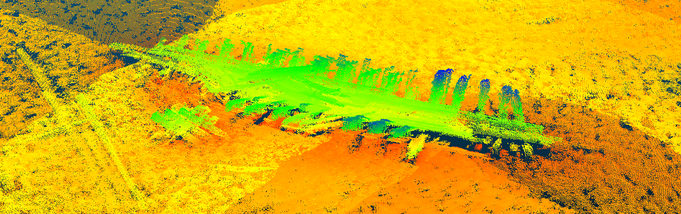
(a) Prior elevation map (INS)

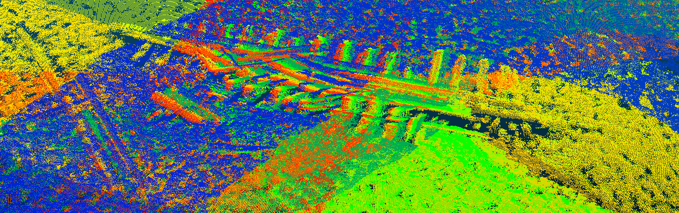
(b) Prior time stamp map (INS)

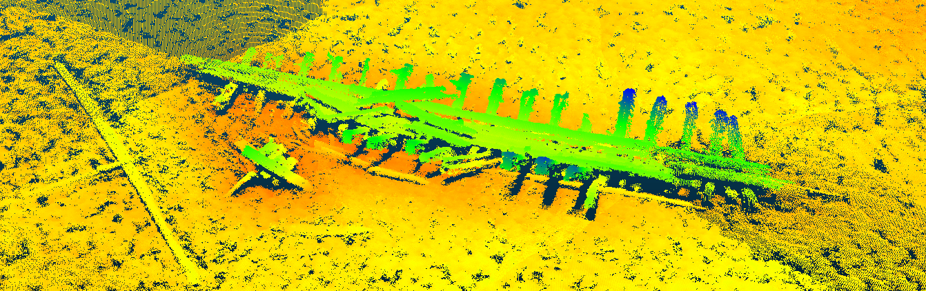
(c) Posterior elevation map (INS+LC)

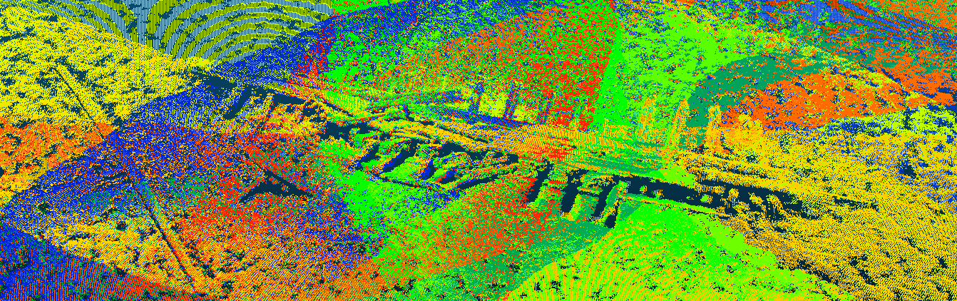
(d) Posterior time stamp map (INS+LC)

Figure B.1: Images of the Wiarton shipwreck area, comparing the prior INS point cloud map in the top row to the posterior INS+LC point cloud map in the bottom row. In the right column, colour denotes relative trajectory time, from low (blue) to high (red). The time stamp plots are included to highlight the many passes involved in generating the final point cloud map.

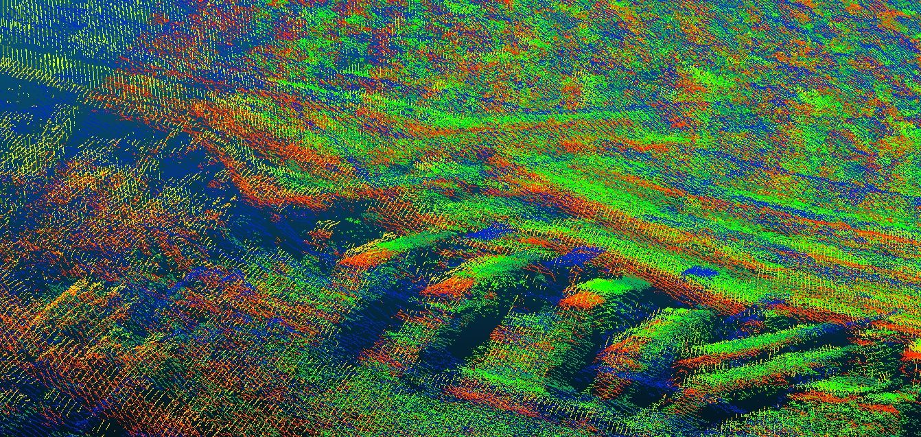
(a) Prior time stamp map (INS), zoom

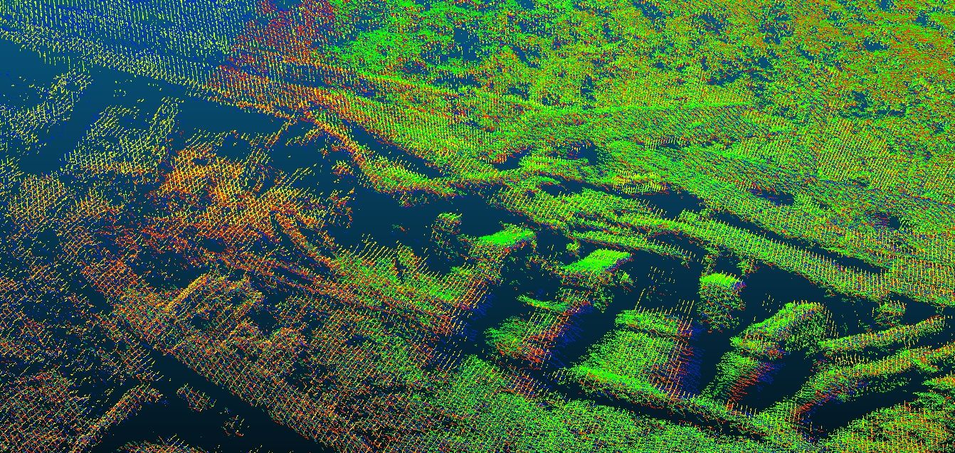
(b) Posterior time stamp map (INS+LC), zoom

Figure B.2: A zoom of the shipwreck area, corresponding to the images in Figure 1. The INS+LC solution on the right delivers a markedly more crisp, self-consistent point cloud map, suitable for inspection and metrology work.

References

- [1] Ayoung Kim and Ryan M Eustice “Real-time visual SLAM for autonomous underwater hull inspection using visual saliency” In IEEE Trans. Robot. 29.3 IEEE, 2013, pp. 719–733
- [2] Sudharshan Suresh, Eric Westman and Michael Kaess “Through-water stereo SLAM with refraction correction for AUV localization” In IEEE Robot. Autom. Lett. (RAL) 4.2 IEEE, 2019, pp. 692–699
- [3] Sharmin Rahman, Alberto Quattrini Li and Ioannis Rekleitis “SVIn2: An underwater SLAM system using sonar, visual, inertial, and depth sensor” In Proc. IEEE/RSJ Int. Conf. Intell. Robots Syst. (IROS), 2019, pp. 1861–1868 IEEE
- [4] Chris Roman and Hanumant Singh “A self-consistent bathymetric mapping algorithm” In J. Field Robot. 24.1-2 Wiley Online Library, 2007, pp. 23–50
- [5] Stephen Barkby, Stefan B Williams, Oscar Pizarro and Michael V Jakuba “A featureless approach to efficient bathymetric SLAM using distributed particle mapping” In J. Field Robot. 28.1 Wiley Online Library, 2011, pp. 19–39
- [6] Paul Ozog, Nicholas Carlevaris-Bianco, Ayoung Kim and Ryan M Eustice “Long-term Mapping Techniques for Ship Hull Inspection and Surveillance using an Autonomous Underwater Vehicle” In J. Field Robot. 33.3 Wiley Online Library, 2016, pp. 265–289
- [7] Albert Palomer, Pere Ridao and David Ribas “Inspection of an underwater structure using point-cloud SLAM with an AUV and a laser scanner” In J. Field Robot. 36.8 Wiley Online Library, 2019, pp. 1333–1344
- [8] Thomas Hitchcox and James Richard Forbes “A Point Cloud Registration Pipeline using Gaussian Process Regression for Bathymetric SLAM” In Proc. IEEE/RSJ Int. Conf. Intell. Robots Syst. (IROS), 2020, pp. 4615–4622 IEEE
- [9] Liam Paull, Sajad Saeedi, Mae Seto and Howard Li “AUV Navigation and Localization: A Review” In IEEE J. Ocean. Eng. 39.1 IEEE, 2014, pp. 131–149
- [10] Michael V Jakuba et al. “Long-baseline acoustic navigation for under-ice autonomous underwater vehicle operations” In J. Field Robot. 25.11-12 Wiley Online Library, 2008, pp. 861–879
- [11] Cesar Cadena et al. “Past, present, and future of simultaneous localization and mapping: Toward the robust-perception age” In IEEE Trans. Robot. 32.6 IEEE, 2016, pp. 1309–1332
- [12] Yaakov Bar-Shalom, X Rong Li and Thiagalingam Kirubarajan “Estimation with Applications to Tracking and Navigation: Theory Algorithms and Software” John Wiley & Sons, 2004
- [13] “SPRINT-Nav datasheet”, 2021 Sonardyne URL: https://www.sonardyne.com/wp-content/uploads/2021/07/Sonardyne_8253_SPRINT_Nav.pdf
- [14] Rainer Kümmerle et al. “g2o: A general framework for graph optimization” In Proc. IEEE Int. Conf. Robot. Autom. (ICRA), 2011, pp. 3607–3613 IEEE
- [15] Michael Kaess et al. “iSAM2: Incremental smoothing and mapping using the Bayes tree” In Int. J. Robot. Res. 31.2 Sage Publications Sage UK: London, England, 2012, pp. 216–235
- [16] Frank Dellaert and Michael Kaess “Factor graphs for robot perception” In Foundations Trends Robot. 6.1-2 Now Publishers, Inc., 2017, pp. 1–139
- [17] Stephen Barkby, Stefan B Williams, Oscar Pizarro and Michael V Jakuba “Bathymetric particle filter SLAM using trajectory maps” In Int. J. Robot. Res. 31.12 SAGE Publications Sage UK: London, England, 2012, pp. 1409–1430
- [18] Albert Palomer, Pere Ridao and David Ribas “Multibeam 3D underwater SLAM with probabilistic registration” In Sensors 16.4 Multidisciplinary Digital Publishing Institute, 2016, pp. 560
- [19] Hordur Johannsson et al. “Imaging sonar-aided navigation for autonomous underwater harbor surveillance” In Proc. IEEE/RSJ Int. Conf. Intell. Robots Syst. (IROS), 2010, pp. 4396–4403 IEEE
- [20] Ayoung Kim and Ryan M Eustice “Active visual SLAM for robotic area coverage: Theory and experiment” In Int. J. Robot. Res. 34.4-5 SAGE Publications Sage UK: London, England, 2015, pp. 457–475
- [21] Pedro V Teixeira, Michael Kaess, Franz S Hover and John J Leonard “Underwater inspection using sonar-based volumetric submaps” In Proc. IEEE/RSJ Int. Conf. Intell. Robots Syst. (IROS), 2016, pp. 4288–4295 IEEE
- [22] Jie Li, Michael Kaess, Ryan M Eustice and Matthew Johnson-Roberson “Pose-graph SLAM using forward-looking sonar” In IEEE Robot. Autom. Lett. (RAL) 3.3 IEEE, 2018, pp. 2330–2337
- [23] Timothy D Barfoot “State Estimation for Robotics” Cambridge University Press, 2017
- [24] Joan Sola, Jeremie Deray and Dinesh Atchuthan “A micro Lie theory for state estimation in robotics” In arXiv preprint arXiv:1812.01537, 2018
- [25] Jonathan Arsenault “Practical Considerations and Extensions of the Invariant Extended Kalman Filtering Framework”, 2019
- [26] Gregory S Chirikjian “Stochastic Models, Information Theory, and Lie Groups, Volume 2: Analytic Methods and Modern Applications” Springer Science & Business Media, 2011
- [27] Carl Edward Rasmussen and Christopher K I Williams “Gaussian Processes for Machine Learning” MIT press, 2006
- [28] Sean Anderson and Timothy D Barfoot “Full STEAM ahead: Exactly sparse Gaussian process regression for batch continuous-time trajectory estimation on SE(3)” In Proc. IEEE/RSJ Int. Conf. Intell. Robots Syst. (IROS), 2015, pp. 157–164 IEEE
- [29] Tim D Barfoot, Chi Hay Tong and Simo Särkkä “Batch Continuous-Time Trajectory Estimation as Exactly Sparse Gaussian Process Regression” In Robot.: Sci. Syst. (RSS) 10, 2014 Citeseer
- [30] Ethan Eade “Lie groups for computer vision”, 2014
- [31] Haoyang Ye, Yuying Chen and Ming Liu “Tightly coupled 3D lidar inertial odometry and mapping” In Proc. IEEE Int. Conf. Robot. Autom. (ICRA), 2019, pp. 3144–3150 IEEE
- [32] Jiarong Lin and Fu Zhang “A fast, complete, point cloud based loop closure for LiDAR odometry and mapping” In arXiv preprint arXiv:1909.11811, 2019
- [33] Philippe Babin, Philippe Giguère and François Pomerleau “Analysis of Robust Functions for Registration Algorithms” In Proc. IEEE Int. Conf. Robot. Autom. (ICRA), 2019, pp. 1451–1457 IEEE
- [34] Yang Chen and Gérard Medioni “Object modelling by registration of multiple range images” In Image Vis. Comput. 10.3 Elsevier, 1992, pp. 145–155
- [35] Kok-Lim Low “Linear least-squares optimization for point-to-plane ICP surface registration” In Chapel Hill, University of North Carolina 4.10, 2004, pp. 1–3
- [36] José Neira and Juan D Tardós “Data association in stochastic mapping using the joint compatibility test” In Trans. Robot. Autom. 17.6 IEEE, 2001, pp. 890–897
- [37] Heng Yang, Jingnan Shi and Luca Carlone “TEASER: Fast and Certifiable Point Cloud Registration” In IEEE Trans. Robot. 37.2 Springer, 2020, pp. 314–333
- [38] Radu Bogdan Rusu, Nico Blodow and Michael Beetz “Fast point feature histograms (FPFH) for 3D registration” In Proc. IEEE Int. Conf. Robot. Autom. (ICRA), 2009, pp. 3212–3217 IEEE
- [39] David G Lowe “Distinctive image features from scale-invariant keypoints” In Int. J. Comput. Vis. 60.2 Springer, 2004, pp. 91–110
- [40] R. B. Rusu and S. Cousins “3D is here: Point Cloud Library (PCL)” In Proc. IEEE Int. Conf. Robot. Autom. (ICRA), 2011, pp. 1–4 IEEE DOI: 10.1109/ICRA.2011.5980567
- [41] Yu Zhong “Intrinsic shape signatures: A shape descriptor for 3D object recognition” In IEEE Int. Conf. Comput. Vis. (ICCV) Workshops, 2009, pp. 689–696 IEEE
- [42] Ivan Sipiran and Benjamin Bustos “Harris 3D: A robust extension of the Harris operator for interest point detection on 3D meshes” In Vis. Comput. 27.11 Springer, 2011, pp. 963–976
- [43] Federico Tombari, Samuele Salti and Luigi Di Stefano “Unique signatures of histograms for local surface description” In Eur. Conf. Comput. Vis., 2010, pp. 356–369 Springer
- [44] Qian-Yi Zhou, Jaesik Park and Vladlen Koltun “Fast global registration” In Eur. Conf. Comput. Vis., 2016, pp. 766–782 Springer
- [45] Martin A Fischler and Robert C Bolles “Random sample consensus: a paradigm for model fitting with applications to image analysis and automated cartography” In Commun. ACM 24.6 ACM New York, NY, USA, 1981, pp. 381–395
- [46] Duowen Qian, Guillaume Charland-Arcand and James Richard Forbes “TWOLATE: Total Registration of Point-Clouds Using a Weighted Optimal Linear Attitude and Translation Estimator” In Proc. IEEE Conf. Control Technol. Appl., 2020, pp. 43–48 IEEE
- [47] Mark Pauly, Markus Gross and Leif P Kobbelt “Efficient simplification of point-sampled surfaces” In IEEE Vis., 2002, pp. 163–170 IEEE
- [48] Thomas Hitchcox and James Richard Forbes “Comparing Robust Cost Functions for Bathymetric Point Cloud Registration” In IEEE/OES Auton. Underwater Veh. Symp. (AUV), 2020, pp. 1–6 IEEE
- [49] Jeff M Phillips, Ran Liu and Carlo Tomasi “Outlier robust ICP for minimizing fractional RMSD” In Int. Conf. 3D Digital Imag. Model., 2007, pp. 427–434 IEEE
- [50] François Pomerleau, Francis Colas, Roland Siegwart and Stéphane Magnenat “Comparing ICP variants on real-world data sets: Open-source library and experimental protocol” In Auton. Robots 34.3 Springer, 2013, pp. 133–148
- [51] Martin Brossard, Silvére Bonnabel and Axel Barrau “A New Approach to 3D ICP Covariance Estimation” In IEEE Robot. Autom. Lett. (RAL) 5.2 IEEE, 2020, pp. 744–751
- [52] Jay Farrell “Aided Navigation: GPS with High Rate Sensors” McGraw-Hill, Inc., 2008
- [53] Charles Van Loan “Computing integrals involving the matrix exponential” In IEEE Trans. Autom. Control 23.3 IEEE, 1978, pp. 395–404
- [54] Niko Sünderhauf and Peter Protzel “Switchable constraints for robust pose graph SLAM” In Proc. IEEE/RSJ Int. Conf. Intell. Robots Syst. (IROS), 2012, pp. 1879–1884 IEEE
- [55] Gim Hee Lee, Friedrich Fraundorfer and Marc Pollefeys “Robust pose-graph loop-closures with expectation-maximization” In Proc. IEEE/RSJ Int. Conf. Intell. Robots Syst. (IROS), 2013, pp. 556–563 IEEE
- [56] Heng Yang, Pasquale Antonante, Vasileios Tzoumas and Luca Carlone “Graduated non-convexity for robust spatial perception: From non-minimal solvers to global outlier rejection” In IEEE Robot. Autom. Lett. (RAL) 5.2 IEEE, 2020, pp. 1127–1134
- [57] Thomas Hitchcox and James Richard Forbes “Mind the Gap: Norm-Aware Adaptive Robust Loss for Multivariate Least-Squares Problems” In IEEE Robot. Autom. Lett. (RAL) 7.3 IEEE, 2022, pp. 7116–7123
- [58] Joshua G Mangelson, Maani Ghaffari, Ram Vasudevan and Ryan M Eustice “Characterizing the uncertainty of jointly distributed poses in the Lie algebra” In IEEE Trans. Robot. 36.5 IEEE, 2020, pp. 1371–1388
- [59] Rainer Kümmerle et al. “On measuring the accuracy of SLAM algorithms” In Auton. Robots 27.4 Springer, 2009, pp. 387–407
- [60] Chris Roman and Hanumant Singh “Consistency Based Error Evaluation for Deep Sea Bathymetric Mapping with Robotic Vehicles” In Proc. IEEE Int. Conf. Robot. Autom. (ICRA), 2006, pp. 3568–3574 IEEE
- [61] Tim Yuqing Tang, David Juny Yoon and Timothy D Barfoot “A white-noise-on-jerk motion prior for continuous-time trajectory estimation on SE(3)” In IEEE Robot. Autom. Lett. (RAL) 4.2 IEEE, 2019, pp. 594–601
- [62] Patryk Cieślak “Stonefish: An Advanced Open-Source Simulation Tool Designed for Marine Robotics, With a ROS Interface” In OCEANS, 2019, pp. 1–6 IEEE
- [63] Brian Curless and Marc Levoy “A volumetric method for building complex models from range images” In SIGGRAPH, 1996, pp. 303–312
- [64] Gerhard Kurz, Matthias Holoch and Peter Biber “Geometry-based Graph Pruning for Lifelong SLAM” In Proc. IEEE/RSJ Int. Conf. Intell. Robots Syst. (IROS), 2021, pp. 3313–3320 IEEE
- [65] Pierre Tétreault, Jan Kouba, Pierre Héroux and Patrick Legree “CSRS-PPP: an internet service for GPS user access to the Canadian Spatial Reference Frame” In Geomatica 59.1 Canadian Science Publishing, 2005, pp. 17–28
- [66] Reha Metin Alkan, Serdar Erol, I Murat Ozulu and Veli Ilci “Accuracy comparison of post-processed PPP and real-time absolute positioning techniques” In Geomatics, Nat. Hazards Risk 11.1 Taylor & Francis, 2020, pp. 178–190
- [67] Jeremy N Wong, David J Yoon, Angela P Schoellig and Timothy D Barfoot “A Data-Driven Motion Prior for Continuous-Time Trajectory Estimation on SE(3)” In IEEE Robot. Autom. Lett. (RAL) 5.2 IEEE, 2020, pp. 1429–1436
- [68] Timothy D Barfoot, James R Forbes and David J Yoon “Exactly sparse Gaussian variational inference with application to derivative-free batch nonlinear state estimation” In Int. J. Robot. Res. 39.13 SAGE Publications Sage UK: London, England, 2020, pp. 1473–1502