Stochastics of DNA Quantification
1 Abstract
A common approach to quantifying DNA involves repeated cycles of DNA amplification. This approach, employed by the polymerase chain reaction (PCR), produces outputs that are corrupted by amplification noise, making it challenging to accurately back-calculate the amount of input DNA. Standard mathematical solutions to this back-calculation problem do not take adequate account of such noise and are error-prone. Here, we develop a parsimonious mathematical model of the stochastic mapping of input DNA onto experimental outputs that accounts, in a natural way, for amplification noise. We use the model to derive the probability density of the quantification cycle, a frequently reported experimental output, which can be fit to data to estimate input DNA. Strikingly, the model predicts that a sample with only one input DNA molecule has a 4% chance of testing positive, which is 25-fold lower than assumed by a standard method of interpreting PCR data. We provide formulae for calculating both the limit of detection and the limit of quantification, two important operating characteristics of DNA quantification methods that are frequently assessed by using ad-hoc mathematical techniques. Our results provide a mathematical foundation for the rigorous analysis of DNA quantification.
2 Introduction
The quantification of genomic targets is of interest in a large variety of applications in biology, biotechnology and medicine, from determining an individual’s disease status to detecting minute changes in gene expression profiles occurring across space and time (eg. [1, 2]). This is typically achieved by converting non-DNA genomic targets into DNA, which is then amplified to enable its quantification. In principle, this allows even small numbers of genomic targets to be accurately measured. However, in practice, the DNA amplification process, being stochastic, generates outputs that contain noise. Accurate measurement, therefore, requires an adequate, quantitative understanding of this noise. Thus far, this has proved challenging to achieve.
A specific and very popular instance of a DNA quantification method is the real-time polymerase chain reaction (PCR) [3, 4]. In PCR, DNA molecules are repeatedly amplified in a cyclic manner. As they are amplified, fluorescently labeled nucleotides are incorporated into the newly formed DNA molecules, increasing the overall fluorescence emitted. The resulting fluorescence profile is used to determine the quantification cycle (denoted or value), at which the number of molecules exceeds a defined threshold, called the quantification threshold. A PCR reaction is considered to be positive if its value is less than or equal to the maximum possible cycle. Despite the fact that the value is only an indirect readout of the number of input DNA molecules, it is often the only reported output of PCR experiments. A variant of conventional PCR, called digital PCR [5], uses the fraction of positive reactions to estimate the number of input DNA molecules. To this end, it assumes that a reaction is positive if and only if it contains at least one target molecule. It is unclear under what conditions this assumption is valid, and when it must be discarded in favor of a more realistic alternative.
Here we describe a parsimonious mathematical model that is useful for analysing the DNA quantification process, and for guiding the interpretation of experimental outputs. We use PCR as an example, although our analysis is applicable to other methods such as loop-mediated isothermal amplification of DNA [6]. Experiments indicate that the PCR process exhibits different phases, characterized by different efficiencies of DNA amplification. Therefore, we construct a mathematical model of a PCR process with an arbitrary number of phases, each with its own amplification efficiency. We use this model to obtain the following results:
-
•
We derive the generating function for the probability distribution of the number of molecules found in a PCR experiment at an arbitrary time . We also derive the probability density function (pdf), mean, variance, and cumulative density function (cdf) of the values produced by such an experiment. Either the pdf or the cdf can be fit to PCR data to estimate the number of input DNA molecules.
-
•
In the simplest instance of our model – a single-phase PCR model that accounts for amplification noise but not for (upstream) DNA sampling noise – the mean value, given by , is well approximated by [7] when , where is the number of input molecules, (defined on a base- scale) is the amplification efficiency, is the quantification threshold, and denotes the digamma function.
-
•
We provide a formula for calculating the limit of detection (LoD) of a PCR experiment, that is, the smallest number of input molecules that can be detected with a failure rate not exceeding . Using a single-phase PCR model, we find that when , the LoD increases from 3, the value determined while accounting for sampling noise only, to 10 when both sampling noise and amplification noise (with set to 95% of the maximum possible efficiency, m.p.e.) are considered. The LoD increases as decreases, doubling to 20 at 90% m.p.e. This illustrates the under-appreciated, dramatic effect that amplification efficiency has on the LoD.
-
•
We provide a formula for calculating the limit of quantification (LoQ) of a PCR experiment, that is, the smallest number of molecules that can be quantified with a defined level of precision and a given maximum failure rate . Counter-intuitively, the single-phase PCR model predicts that the LoQ does not depend on amplification efficiency. When , the LoQ increases from , obtained when up to a two-fold deviation from the expected number of input molecules is allowed, to 820, when at most a 10% deviation is allowed. This indicates that 10 or fewer molecules cannot be measured with a better than 2-fold error more than 95% of the time.
-
•
The model indicates that a key assumption commonly used when interpreting digital PCR data – that a PCR experiment with only one input molecule will always produce a positive outcome – is invalid under a wide range of conditions. Even when the amplification efficiency is set to a high value of 95% m.p.e, the probability that such an experiment will yield a positive outcome is predicted to be 4%. We describe two different approaches by which accurate estimates of the number of input DNA molecules may be obtained from digital PCR data.
It should be noted that there have been previous attempts to improve the interpretation of PCR data through mathematical modeling. The classical approach to estimating the amount of DNA found in a focal sample involves comparing data generated by that sample versus data obtained from a reference sample containing either a known or an unknown amount of DNA [8]. The need for a reference sample with a known amount of DNA, the determination of which is itself subject to experimental error, makes accurate absolute quantification of DNA found in the focal sample challenging. An alternative approach involves fitting mathematical models, mostly phenomenological in their construction, to PCR data generated by the focal sample alone [4, 8, 9, 10, 11]. See [12] for a comparison of various methods based on this approach. None of these methods provides an adequate accounting of how amplification noise shapes PCR data.
The remainder of this paper is organized as follows: We provide an overview of the model’s structure in Section 3.1 and present our main mathematical results in Sections 3.2 and 3.3. We apply these results to compute the LoD and LoQ in Section 3.4, and we investigate how amplification noise complicates the accurate interpretation of digital PCR data in Section 3.5. We summarize the results and discuss other applications of our methods in Section 4. To improve readability, we only present mathematical proofs and detailed calculations in the Appendix (Section 5.1).
3 Results
3.1 Preliminaries
We model the PCR process as a continuous-time, discrete-state Markov jump process [13] evolving up to time . This representation of the PCR process is based on the facts that (1) the primary products of PCR reactions, DNA molecules, are countable, and (2) what happens in the next cycle of the reaction is conditionally independent of what happened in the past given the present state of the reaction. Our decision to make time continuous (rather than discrete) is based on the fact that experimentally measured values are positive real numbers. As a consequence, reaction rates are defined in base instead of base (expected for a discrete-time PCR process), but it is straightforward to convert between these two bases.
We divide the time interval of the PCR process into non-overlapping subintervals , each one corresponding to a distinct phase of the process and associated with the probabilistic state transition rate , . These transition rates govern the efficiency of DNA amplification. We derive the probability generating function [14] for the number of target molecules found at an arbitrary time . We use this generating function to derive the corresponding probability distribution and, importantly, the probability density function (pdf) of the value. We derive the pdf in two different cases, namely
-
1.
when the initial state of the PCR process is deterministic, and the PCR phase lengths and amplification efficiencies are given; and
-
2.
when the initial state is Poisson-distributed, and the phase lengths and amplification efficiencies are given.
To illustrate the mathematical ideas, we will report calculations and simulations based on a single-phase model. We argue that this simpler instance of our model is sufficient for analysing a large variety of real-world PCR experiments. In principle, each PCR experiment can be divided into the following three amplification rate-dependent phases: a pre-exponential phase, in which the amplification rate is sub-exponential; an exponential phase; and a post-exponential phase where the rate slows down as DNA molecules saturate the reagents required for their further amplification. However, in practice, the usual output of PCR experiments – the value – is determined as soon as the PCR process enters the exponential phase, meaning that dynamics occurring in the pre-exponential phase primarily determine this particular outcome. Therefore, for the purposes of understanding the factors that shape the value and its statistics, and evaluating related operating characteristics of PCR, a single-phase model appears sufficient. Accordingly, when applicable, we highlight the forms taken by our mathematical equations in the case of a single-phase model. In addition, we estimate the LoD and LoQ using a single-phase model (Section 3.4), which we also apply to critique the standard method of interpreting digital PCR data (Section 3.5).
3.2 Case 1: A PCR process with a deterministic initial state
3.2.1 Probability generating function for the number of molecules
Theorem 1.
Let be a continuous-time Markov process with phases, a countable state space , phase-specific transition rates and state transition probability given by
| (1) |
where denotes the indicator function and denotes the Kronecker delta function. If the process starts with molecules, then the probability generating function for the number of molecules present at time , , is given by
| (2) |
where
| (3) |
denotes the i’th phase and , , is its length.
The proof of this theorem is given in Section 5.1.1. We will now use the theorem to derive the probability distribution of the number of molecules found at time .
3.2.2 Probability distribution of the number of molecules
Corollary 1.
The proof of this corollary is given in Section 5.1.2. We will now use this corollary to derive the pdf, mean, variance and cdf of the value.
3.2.3 pdf, mean and variance of the Ct value
Let be the value of the PCR process described in Theorem 1. By definition, is the time at which the number of molecules reaches the quantification threshold, which we denote by . Let . In the Appendix [Section 5.1.5], we show that, given , and , the pdf of has the following form:
| (5) |
where is the incomplete Beta function, is given by (3), and
| (6) |
For the single-phase PCR process, , so the pdf is given by
| (7) |
The mean value is given by (see Section 5.1.5)
| (8) |
where is the regularized generalized hypergeometric function.
For the single-phase process, the mean is given by
| (9) |
Observe that when , the right-hand-side of (9) is well-approximated by . The latter expression is commonly used to approximate the mean value. For example, it was used in [7] to estimate PCR amplification efficiency from data.
The variance of the value is given by , where is given by (85). For the single-phase process, the variance is given by
| (10) |
where is the second polygamma function (also called the trigamma function).
Finally, the cdf of the value is given by [see Section 5.1.5]
| (11) |
For the single-phase process, the cdf is given by
| (12) |
where is the regularized incomplete Beta function. Sampling from this cdf is relatively straightforward: A random value is obtained as follows:
| (13) |
where is sampled uniformly at random from the interval and is the inverse of the regularized incomplete Beta function. To find a value that corresponds to a quantile , is substituted for .
To estimate , either the pdf or the cdf of can be fit to data. Alternatively, the posterior density of conditioned on can be computed. In Section 5.1.5, we show that, for the single-phase process, it is given by
| (14) |
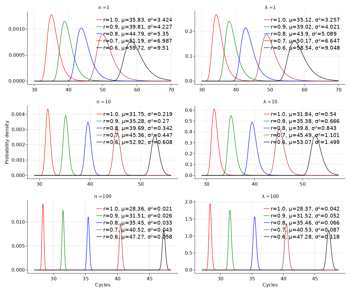
In Figure 1, we illustrate the shape of the single-phase pdf for different numbers of input molecules and different amplification efficiencies. To this end, we set (a common upper-bound for the duration of real-world PCR experiments) and , which is equal to the number of molecules expected after cycles under perfect amplification conditions (a sample that contains only one, perfectly amplified input molecule is expected to reach the quantification threshold, , at time ). We vary the efficiency from 60% m.p.e. (equivalent to setting ) to 100% m.p.e. The pdf has a bell shape, the location and width of which are governed by both the efficiency and the number of input molecules (Figure 1, left panel). Higher efficiencies or larger numbers of input molecules produce smaller mean values, smaller variances, and narrower pdfs. In contrast, lower efficiencies or smaller numbers of input molecules produce larger mean values, larger variances, and wider pdfs (Figure 1, left panel). In fact, Equation (5) predicts that in the limit as the efficiency goes to 0, the pdf will become flat as it will map every value to 0.
3.3 Case 2: A PCR process with a Poisson-distributed initial state
3.3.1 Probability generating function for the number of molecules
Theorem 2.
Let be the continuous-time Markov process described in Theorem 1. If, instead of starting with a precisely known number of input DNA molecules, the initial state of the process is Poisson-distributed with mean , then the probability generating function for the state of the process at a future time is given by
| (15) |
where is given by (3).
3.3.2 Probability distribution of the number of molecules
Corollary 2.
The proof of this corollary is provided in Section 5.1.4. It is interesting to note that from the proof emerged the following combinatorial triangle, which is related to the well-known Narayana triangle [15]:
| 1 | 1 | |||||
|---|---|---|---|---|---|---|
| 2 | 1 | 2 | ||||
| 3 | 1 | 6 | 6 | |||
| 4 | 1 | 12 | 36 | 24 | ||
| 5 | 1 | 20 | 120 | 240 | 120 | |
| 1 | 2 | 3 | 4 | 5 | ||
| . | ||||||
The entries of this triangle, given by
| (17) |
count the number of ways of obtaining molecules by replicating a randomly selected subset of molecules. is related to the Narayana numbers by
We will now use this corollary to derive the pdf of the value together with the mean, variance and cdf.
3.3.3 pdf, mean and variance of the value
Let be the value of the PCR process described in Theorem 2. As noted earlier, the value is the time at which the number of DNA molecules found in the process reaches the quantification threshold, which we denote by . In the Appendix [Section 5.1.6], we show that the pdf of is given by
| (18) |
where is given by (6), is given by (3), is the hypergeometric function (also called the Kummer confluent hypergeometric function of the first kind).
For the single-phase process, the pdf is given by [see Section 5.1.6]
| (19) |
For the single-phase process, the mean and variance are, respectively, given by [see Section 5.1.6]
| (21) |
| (22) |
The cdf of the value is given by [see Section 5.1.6]
| (23) |
For the single-phase process, the cdf is given by
| (24) |
To estimate , either the pdf or the cdf of can be fit to data. Alternatively, the posterior density of conditioned on can be computed. In Section 5.1.6, we show that, for the single-phase process, it is given by
| (25) |
where and denotes the Riemann zeta function.
Note that, because they result from calculating expectations over the Poisson distribution, the summations found in Equations (18) - (25) can be truncated at any value of without a loss of accuracy.
In Figure 1, we illustrate the shape of the single-phase pdf for different values of and different amplification efficiencies. As was the case for the PCR process with a deterministic initial state (Figure 1, left panel), the pdf also has a bell shape (Figure 1, right panel). Its location and width are governed by both the efficiency and . Consistent with expectations, higher efficiencies or larger values of produce smaller mean values, smaller variances, and narrower pdfs (Figure 1, right panel). In contrast, lower efficiencies or smaller values of produce larger mean values, larger variances, and wider pdfs.
3.4 Limit of detection and limit of quantification
We will now demonstrate theoretically how the mathematical framework we have developed can be applied to achieve certain operationally important objectives. In particular, it is often of interest to quantify the limit of detection (LoD) of a particular instance of the PCR method (henceforth referred to as “PCR protocol”). The LoD of a PCR protocol is the smallest number of molecules that it can detect with a failure rate not exceeding a defined threshold ( is also called the significance level). Protocols with smaller LoDs are in general preferred to those with larger LoDs. Ideally, the LoD should be either equal to or smaller than the number of input DNA molecules expected in the considered sample. Another important operational objective is to determine a PCR protocol’s limit of quantification (LoQ) – i.e. the smallest number of molecules that it can estimate with a given level of precision (measured here using the parameter ) and a given maximum failure rate . When a -fold change in the number of target molecules needs to be detected, the protocol should have an LoQ with precision . The methods available for estimating LoD and LoQ are laborious [16] and frequently rely on certain ad-hoc mathematical approximations [16, 17], which we would like to circumvent by developing and executing mathematically precise statements of the estimation problem.
We begin with the LoD estimation problem. For the PCR process with a deterministic initial state, the LoD can be expressed as follows:
| (26) | |||||
where is given by (11) and is the maximum practical duration of the PCR process. For the process with a Poisson-distributed initial state, is replaced by .
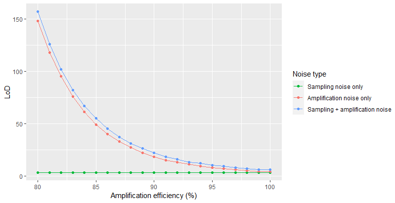
In Supplementary Figure 5.1, we show how the LoD varies with amplification efficiency in a single-phase process with either a deterministic or a Poisson-distributed initial state. In the former case, the process contains amplification noise but no sampling noise while in the latter case it contains both sampling noise and amplification noise. For comparison, we also show the LoD in a process with sampling noise, modeled by using the Poisson distribution, but without amplification noise. The LoD is lowest in a process with sampling noise alone (LoD = 3 molecules) and it is highest when both sampling noise and amplification noise are present (LoD ranges from 6 molecules, at 100% of maximum possible efficiency or m.p.e, to 157 molecules, at 80% m.p.e). A process with amplification noise but without sampling noise has an intermediate LoD. In these computational examples, the parameters of the equation used to estimate the LoQ are perfectly known, and this makes it possible to obtain perfect knowledge of the LoD. In real-world applications, the parameter values will be associated with uncertainty, which will, in a quantifiable way, make uncertain the LoD estimates.
We now turn our attention to the problem of estimating the LoQ in a PCR process with a deterministic initial state. Suppose that a value is generated by such a process and then used to obtain an estimate, denoted , of the number of input molecules. Let be the actual number of input molecules. We want to calculate the probability that, for any data generated by the same process, will not differ from by more than a factor . We define the LoQ as the smallest value of for which this probability exceeds . Specifically, the LoQ is given by
| (27) | |||||
where (respectively ) denotes the largest (respectively smallest) integer less than (respectively greater than) or equal to .
Focusing on the single-phase process, to obtain , we marginalize the right-hand-side of (14) with respect to and then take the sum from to , yielding [see Section 5.1.5]
| (28) | |||||
Strikingly, while Equation (28) depends on both and , it does not depend on the amplification efficiency . In the Appendix [see Equation (130)], we follow a similar procedure to obtain , the probability that, for any data generated by a single-phase PCR process with a Poisson-distributed initial state, the estimated value of, denoted , will not differ from the actual value by more than a factor .
Setting and allowing at most a 10% deviation of from (corresponding to setting ) results in an LoQ of 820 molecules. The LoQ decreases to 146 molecules when a deviation of up to 25% from expectation is allowed (corresponding to ), and to 43 molecules when the allowable deviation increases to 50% (corresponding to ). The analysis suggests that at the considered 5% failure rate, 10 input molecules can be detected with an error of at least 200%, that is, a fold deviation from (corresponding to ). Because these calculations do not account for sampling noise, they provide only a lower-bound for the LoQ that is achievable at the considered failure rate and level of precision (). As noted earlier, in real-world applications the parameters of the equation used to estimate LoQ will be imperfectly known, and this will determine the amount of uncertainty associated with the estimated LoQ.
3.5 Amplification noise determines digital PCR outcomes
As noted earlier, digital PCR is a variant of conventional PCR that was developed to improve the quantification of DNA. In digital PCR, a sample master mix (containing an unknown number of input DNA molecules together with all the reagents required for DNA replication) is uniformly distributed into hundreds (and sometimes thousands) of physical partitions, which may take the form of droplets or microwells [5]. Each partition is expected to receive zero, one, or more DNA molecules following a Poisson distribution with mean , where is the concentration of the DNA in the original sample, is the partition volume, and is the (known) dilution factor applied to the sample during preparation of the mastermix. PCR reactions are independently and simultaneously run inside each partition, and positive partitions are identified. The resulting data – i.e. the positive or negative outcome of each PCR reaction – are thus digital. The standard method of interpreting these data assumes that partitions that receive at least one target molecule will test positive, and their fraction, , is approximated by , from which is estimated as and then used to estimate .
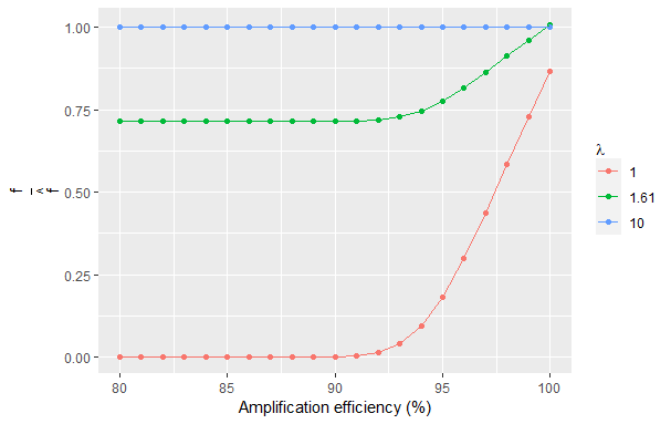
However, according to our model, the assumption that the fraction of positive partitions equals the Poisson probability that a partition receives one or more target molecules is untenable due to the effects of PCR amplification noise. Indeed, setting the amplification efficiency to a reasonably high value of 95% m.p.e (i.e. and using in Equation (24), we predict that 4% of partitions that contain only one molecule will test positive, which is 25-fold smaller than assumed by the Poisson method. In Supplementary Figure 5.2, we compare the fraction of positive partitions calculated using our model [Equation(24)] versus the positive fraction calculated by the Poisson method, for different values of and different amplification efficiencies. We find that the Poisson method over-estimates the fraction of positive partitions for small values of , including the value (1.61) at which the method is expected [18] to produce its most precise estimates of . Only for a relatively large value of (10) do we find the Poisson method’s estimate of the fraction of positive partitions to agree with the noise-adjusted expectation calculated using our model (Supplementary Figure 5.2).
We use our model to investigate how this over-estimation of the fraction of positive partitions affects the accuracy of the estimate of (denoted ) produced by the Poisson method. Setting in Equation (24), we find that
| (29) | |||||
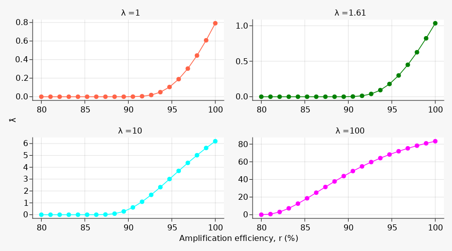
According to Equation (29), depends strongly on the amplification efficiency . equals 0 in the limit as tends to 0. As increases to its maximum possible value of , also increases, approaching . In Figure 2, we illustrate the relationship between and amplification efficiency. Strikingly, for efficiencies lower than 95% m.p.e, is very small, indicating that is markedly under-estimated by the Poisson method. When the efficiency equals 95% m.p.e, increases from (at ) to 69% (at ). Increasing the efficiency to the maximum possible value of 100% m.p.e causes to increase to 80% (at ). These results indicate that the Poisson method is expected to under-estimate because it does not account for amplification noise. Indeed, experimental data show a strong tendency by the method to under-estimate the number of input DNA molecules (eg. see Supplementary Table 6 in [19]).
4 Discussion
The outputs of DNA quantification experiments, including those based on the polymerase chain reaction (PCR), tend to vary within and across different experimental instances, making the results difficult to interpret and limiting their utility beyond the particular contexts in which they are generated. Indeed, various factors are known to contribute to the variability of PCR outputs [20, 21, 22] including the varying complexity of DNA templates and the random distribution of target molecules in the reaction environment; the type of PCR machine and buffer components used; the durations and temperatures of the three thermal cycles of PCR; the binding kinetics of oligonucleotide primers to target DNA; and the stability of DNA polymerase and other PCR reagents. Taylor et. al [22] reviewed the sources of variability in PCR experiments and proposed a stepwise process to minimize such variability in practice.
A common output of a PCR experiment is the quantification cycle (denoted or value), the PCR cycle at which the number of DNA molecules exceeds a defined threshold, called the quantification threshold. The value varies with both the number of input DNA molecules and the PCR amplification efficiency, which in turn varies with the aforementioned experimental variables. It is desirable to deconvolute such variable outputs to estimate the number of input DNA molecules, which is of greatest interest in experiments, by applying mathematical methods that account for the stochasticity that is inherent in the underlying generative process.
We have developed a mathematical approach to modeling DNA quantification that takes into account the underlying stochasticity. We used PCR, the most widely used class of DNA quantification process, to illustrate our mathematical ideas, which are also applicable to a broader class of such processes (eg. [6]). Using the model, we derived the probability generating function for the number of molecules found in a PCR process with either a deterministic or a Poisson-distributed number of input molecules as well as the probability density function (pdf), mean, variance and cumulative density function (cdf) of the value produced by such a process. In contrast to the deterministic case, in which PCR outputs are contaminated only by amplification noise, in the latter case the outputs also contain sampling noise. The equations we derived for these important statistical properties of the PCR process revealed functional relationships between the value and underlying variables that could previously only be accessed by empirical means.
To illustrate our mathematical ideas, we focused on the single-phase PCR process, for which our modeling results take relatively simple mathematical forms. We found that the common assumption that the mean value is a simple logarithmic function of the number of input DNA molecules is correct when is large. For small , corrections are required. An exact mean value is given by , where is the quantification threshold, is the amplification efficiency and denotes the first polygamma function. The variance has the elegant form , where denotes the second polygamma function. Therefore, the variance is strongly dependent on amplification efficiency. This effect is illustrated in Figure 1, which shows that the pdf of the value becomes wider as the amplification efficiency decreases. Interestingly, in this simple case, the coefficient of variation of the value (i.e. the ratio of the standard deviation to the mean) does not depend on amplification efficiency.
Two important numbers that characterize the performance of a PCR process are the limit of detection (LoD) and the limit of quantification (LoQ). The LoD is the smallest number of molecules that can be detected with a failure rate not exceeding a threshold , while LoQ is the smallest number of molecules that can be quantified with a given level of precision (i.e. allowing a defined maximum fold deviation from the true value) and a given maximum failure rate . We provided mathematical formulae for calculating both LoD and LoQ. Close examination of these formulae in the context of a single-phase PCR process revealed that a small reduction of the amplification efficiency may cause a large increase of LoD. For example, when , reducing the efficiency from 95% of the maximum possible efficiency (m.p.e) to 90% m.p.e. caused the LoD to double, from 10 input molecules to 20 molecules. In contrast to LoD, we found that LoQ is independent of efficiency. Allowing up to a 2-fold difference between and its estimate results in an LoQ of 10 molecules. Reducing the allowed fold difference to 10% increases LoQ to 820 molecules. Our methods may be used to improve significantly the current approaches to estimating LoD and LoQ, which are laborious [16] and frequently rely on certain crude mathematical approximations [16, 17] that can be avoided by using our methods.
Furthermore, we applied our methods to shed light on the effects that amplification noise has on estimates of the expected number of input DNA molecules obtained by the standard method of interpreting digital PCR data. A key assumption of this method is that a PCR reaction will be positive if it contains at least one input DNA molecule. We showed that this assumption is in general invalid because of the stochastic nature of PCR amplification. Stochastic effects are particularly large when is small, which is the regime in which digital PCR preferentially operates. At a high amplification efficiency of 95% m.p.e, we find that the ratio of the fraction of positive digital PCR reactions calculated by the standard method versus the value obtained after accounting for amplification noise is only 18.3% when and it increases to 100% when (Figure 5.2). Accordingly, stochastic effects were found to cause a significant under-estimation of by the standard method. Indeed, at a high efficiency of 95% m.p.e., the standard method is predicted to under-estimate by factors of 8.1, 3.1, and 1.4 when equals 1, 10, and 100, respectively (Figure 2). This is in the same range as empirically observed (eg. [19]).
Using our mathematical methods, the following two different approaches may be used to obtain much more accurate estimates of . Firstly, if values are available from positive digital PCR reactions, then Equation (19) can be fit to those values, using either a likelihood-based or a Bayesian statistical approach, to estimate the most probable value of together with a confidence (or credible) interval for it. Secondly, if only binary (ie. positive or negative) outcomes are available from individual reactions, then the variability of such outcomes can still be exploited to estimate . Specifically, suppose there are different reactions. These can be randomly distributed into groups of reactions each. Assuming a binomial distribution of the number of positive reactions found in each group, their first and second moments are given by and , respectively, where is calculated using (24). These moments contain information about the two free parameters of (i.e. and ), which can be readily extracted to estimate together with a confidence (or credible) interval.
The value is estimated from the fluorescence profiles produced by DNA molecules as they are amplified during PCR. Our mathematical analysis can be straightforwardly extended to obtain a time-dependent probability density of the fluorescence intensity , which can then be fit to fluorescence profiles as an alternative approach to estimating the number of input DNA molecules. Using standard results from probability theory (eg. see [23]), can be derived from both the cumulative distribution function of the number of molecules found in the PCR process at time , [calculated based on Equation (4) or (16)] and the linear relation expected [24] between and . Specifically, can be expressed as
| (30) |
where
| (31) |
, and . We will explore in detail this alternative approach to estimating the number of input DNA molecules in a future paper.
5 Supporting Information
5.1 Appendix
This section contains mathematical proofs and detailed calculations supporting the results presented in Section 3.
5.1.1 Proof of Theorem 1
Proof.
We will prove Theorem 1 by mathematical induction on .
-
•
:
The Chapman-Kolmogorov forward equation corresponding to the single-phase process is given by:(32) where we have set , and is the amplification efficiency associated with the process. To simplify our notation, we will abbreviate by .
We will solve (32) by using a powerful combinatorial device called the probability generating function (pgf) [14]. Recall that the pgf of is defined as:
where is a book-keeping variable.
Multiplying both sides of (32) by and summing over all possible values of yields:
(33) Using
(34) we simplify (33) to obtain
(35) which is a partial differential equation (pde) in .
We will solve (35) by the method of characteristics. To this end, we define new variables
which will transform (35) into the simpler equation
(36) which has the solution
where
This requires that , where is an arbitrary constant. The resulting characteristic equation is given by
which has the solution
Setting , we obtain
(37) and
(38) Substituting (37) and (38) into (35) gives
(39) which has the same form as (36). The solution to (39) is given by
(40) If there are molecules at the start of the process (), then if and otherwise. Therefore,
(41) In (41), the argument of maps onto , implying that
(42) Proof.
-
•
:
There are two amplification phases with rates and , respectively. The first one runs from time to , and the second one runs from to . In the second phase, the probability generating function takes exactly the same general functional form as in the first phase, albeit with a different initial condition. Specifically, we havewith the initial condition (at time )
Using the same procedure as in the case when , we obtain
(45) -
•
We assume the statement is true for , that is
where , and we prove it for . As before, in phase , the generating function has the functional form
At time , by the induction step, we have
Using the same arguments as before, we find that, for ,
(46) and this ends the proof of Theorem 1.
∎
5.1.2 Proof of Corollary 1
Proof.
From Theorem 1, we know that the generating function for is given by
Let and . Then,
is the coefficient of in the power series expansion of , given by
| (47) |
But
| (48) | |||||
Substituting (48) into (47) gives
| (49) |
Let . Then,
| (50) |
The probability of having molecules at time , , is therefore given by
| (51) |
∎
Corollary 4.
Proof.
| (52) | |||||
which equals the right-hand side of (32). ∎
5.1.3 Proof of Theorem 2
Proof.
We prove Theorem (2) by mathematical induction on .
-
•
:
There is only one phase with amplification efficiency . Recall that the Chapman-Kolmogorov forward equation for the dynamics of is given by (32), with the initial conditionUsing the same arguments as above, we can write the generating function for as
(53) with the initial condition
(54) Therefore,
(55) -
•
:
There are two phases with amplification efficiencies and , respectively. The first phase runs from time to , and the second one runs from to . As before, for the probability generating function has the formwith the initial condition (at time )
Therefore,
(56) -
•
We assume the statement is true for , that is
where , and we prove it for .
In phase , the probability generating function has the form
By the induction step, the initial condition (at time ) is given by
Therefore, for , we have
(57) where , and this ends the proof of Theorem 2.
∎
5.1.4 Proof of Corollary 2
Proof.
Recall that is the coefficient of in the power series expansion of the probability generating function given in Theorem 2, that is
| (58) |
Now, let us compute the partial derivatives of with respect to . For brevity, we set
Observe that
and
| (59) | |||||
By closely examining the coefficients of powers of the terms in (59), the following combinatorial triangle emerges
| 1 | ||||||
| 1 | 2 | |||||
| 1 | 6 | 6 | ||||
| 1 | 12 | 36 | 24 | |||
| 1 | 20 | 120 | 240 | 120 | ||
| 1 | 2 | 3 | 4 | 5 | ||
In particular, the ’th entry of the triangle is given by
| (60) |
Thus
| (61) | |||||
Setting in (61) gives the desired result. ∎
Proof.
Differentiate the right-hand-side of Equation (61) with respect to . ∎
We will now derive the probability density function (pdf), mean, variance, and cumulative density function (cdf) of the value. We will consider two different cases, namely:
-
1.
when the initial state of the PCR process is deterministic, and the PCR phase lengths and amplification efficiencies are given; and
-
2.
when the initial state is Poisson-distributed, and the phase lengths and amplification efficiencies are given.
5.1.5 Case 1: The initial state is deterministic, and the phase lengths and amplification efficiencies are given
-
•
General form of the pdf
Consider the PCR process described in Theorem 1. The process begins with cDNA molecules, which are amplified across up to successive phases of lengths at the corresponding amplification efficiencies . By definition, the value is the time at which the number of molecules reaches the quantification threshold, which we denote by . By Bayes’ theorem, a general expression for the pdf of is given by(62) Since is independent of , , and , and is also independent of and of the values taken by the entries of , we re-write the numerator of the right-hand-side of (62) as follows:
(63) Similarly, the denominator of the right-hand-side of (62) can be simplified to
(64) Therefore, (62) can be re-written as
(65) We will derive the pdf, mean, variance, and cdf of the value for a PCR process with an arbitrary number of phases . Without loss of generality, we suppose that . We will assume a uniform prior density for given . As we will demonstrate later, this assumption produces very similar results to those we obtain by assuming a Jeffreys prior [25]. We will state results for the case of a single-phase PCR process whenever these cannot be readily gleaned from the general results.
We will first consider the case when the lengths of the intermediate phases, recorded in the vector , are given. This is useful, for example, when it is of interest to estimate the lengths of such phases from data. We will then show how to marginalize out of the pdf.
-
•
pdf
Using the posterior density given in Equation (65) and the likelihood function given in Corollary 1, we obtain the following functional form for the pdf:(66) where
(67) is a vector of amplification efficiencies, is a vector of phase lengths, and we have used a uniform prior for .
The normalizing constant is given by
(68) Let Then,
(69) where
(70) Therefore, the pdf is given by
(71) For the single-phase process, , so the pdf simplifies to
(72) Note that in some cases (eg. when knowledge of the lengths of individual PCR amplification phases is not of interest), it may be useful to marginalize out of . This can be achieved by using the fact that
(73) where is the domain of .
In addition, note that an alternative formulation of the prior for , based on an approach proposed by Jeffreys [25] for generating priors that are invariant to reparametrization, is the following:
(74) where is the Fisher information of the likelihood function and is given by
where .
Observe that
(76) and
where .
Plugging (76) and (LABEL:temp2) into (LABEL:fisher1), we obtain
(78) Using this prior, and following the steps we used earlier to derive (71), we find that the pdf is given by
(79) which has a similar form as (71).
For simplicity, we will continue to use a uniform prior for .
-
•
Let Then,
(81) where is given by (70), is the first polygamma function (also called the digamma function), and
(82) Note that for the single-phase process, . In this case, using
we find that the mean value is given by
(83) -
•
For the single-phase process, the second moment of the value is given by
(86) where is the second polygamma function (also called the trigamma function). Therefore, the variance is
(87) -
•
cdf
The cdf of the value is given by(88) where
For the single-phase process, the cdf is given by
(90) where is the regularized incomplete Beta function. Because the cdf is in closed analytical form, we can apply the efficient inverse transform method to generate random samples of values as follows:
(91) where is a real number sampled uniformly at random from the interval and is the inverse of the regularized incomplete Beta function. To find a value that corresponds to a quantile , simply replace in Equation (91) by .
-
•
Probability distribution of
We conclude by deriving the probability distribution of , denoted , for the single-phase PCR process. This distribution can be used to estimate from measured values. It can also be used to calculate the LoD and LoQ of a PCR assay, as we demonstrated in the main text. The steps described below can also be used to derive , for a PCR process with an arbitrary number of phases, although this will not yield a closed-form result like we will obtain in the single-phase case.By Bayes’ Theorem, we have
(92) where
(93) The normalizing constant is given by
(94) Let . Then,
(95) Therefore, we have
(96) Suppose that is a value generated by a PCR process with input molecules. If we replace by in Equation (96), then the equation will give the probability that will be obtained as the estimate of based on the data . It is useful – eg. for the purpose of determining the LoQ – to calculate the probability that will be obtained as the estimate of based on any data that can be generated by a PCR process with input molecules. This probability is given by
(97) where, using (96), we have assumed that is conditionally independent of given . Strikingly, (97) does not depend on .
5.1.6 Case 2: The initial state is Poisson-distributed, and the phase lengths and amplification efficiencies are given
-
•
General form of the pdf
Let be the value of the PCR process described in Theorem 2. The process begins with a Poisson-distributed number of input DNA molecules, with mean , which are replicated across up to distinct phases with lengths and amplification efficiencies . As noted earlier, is the time at which the number of molecules reaches the quantification threshold, which we denote by . Let us denote the pdf of by . By Bayes’ theorem, we have(98) However, is independent of , , and , while is also independent of and of the precise values taken by the entries of . Therefore, by following the same steps we used earlier to derive (65), we find that
(99) We will derive the pdf, mean, variance, and cdf by assuming, without loss of generality, that , and then we will specify the functional forms taken by the results in the instructive case when . As before, for simplicity, we will use a uniform prior density for .
-
•
pdf
We derive the pdf of the value by using the general expression given in Equation (99), with the probability distribution of the number of molecules given in Theorem 2 serving as the likelihood. Specifically,(100) (102) (103) (104) (105) (106) where is given by (67), is the hypergeometric function (also called the Kummer confluent hypergeometric function of the first kind), defined as
and denotes the rising factorial, i.e. with .
Therefore, the pdf is given by
(109) Recall that for the single-phase process, , so we have
(110) implying that the pdf is given by
(111) Note that in some cases (eg. when knowledge of the lengths of individual PCR amplification phases is not of interest), it may be useful to marginalize out of . This can be achieved by using the fact that
(112) where is the domain of .
-
•
Let Then,
(114) Therefore
Recall that for the single-phase process, , so
(116) - •
-
•
cdf
The cdf of the value is given by(121) where
For the single-phase process, using (110), we simplify the cdf to obtain
(123) -
•
Probability density of
We conclude by deriving the probability density of , , for the single-phase process. This density can be used to estimate from measured values, and for calculating both the LoD and the LoQ of a PCR process. The steps described below can also be used to derive , for a PCR process with an arbitrary number of phases.By Bayes’ Theorem, we have
(124) where .
The normalizing constant is given by
(125) where is the Riemann zeta function.
Therefore, the probability density of is given by
(126) The probability that takes values between and is given by
(127) where is the incomplete Riemann zeta function.
It follows that the cumulative density function of is given by
(128) As discussed earlier in relation to , Equation (126) can be interpreted as follows: Suppose that a value is produced by a PCR process with expected number of input molecules . If we replace by an estimate , then (126) gives the likelihood of . For practical purposes (eg. to determine the LoQ), it is useful to calculate the probability that will be obtained as the estimate of from any data that can be produced by a PCR process with expected number of input molecules . This probability is given by
where is given by (70) and we have assumed that is conditionally independent of given .
It follows that the -independent probability that will take values between and is given by
(130)
5.2 Supplementary Figures
References
- Wölfel et al. [2020] Roman Wölfel, Victor M Corman, Wolfgang Guggemos, Michael Seilmaier, Sabine Zange, Marcel A Müller, Daniela Niemeyer, Terry C Jones, Patrick Vollmar, Camilla Rothe, et al. Virological assessment of hospitalized patients with covid-2019. Nature, 581(7809):465–469, 2020.
- Wang et al. [1989] Alice M Wang, Michael V Doyle, and David F Mark. Quantitation of mrna by the polymerase chain reaction. Proceedings of the National Academy of Sciences, 86(24):9717–9721, 1989.
- Saiki et al. [1985] Randall K Saiki, Stephen Scharf, Fred Faloona, Kary B Mullis, Glenn T Horn, Henry A Erlich, and Norman Arnheim. Enzymatic amplification of -globin genomic sequences and restriction site analysis for diagnosis of sickle cell anemia. Science, 230(4732):1350–1354, 1985.
- Higuchi et al. [1993] Russell Higuchi, Carita Fockler, Gavin Dollinger, and Robert Watson. Kinetic pcr analysis: real-time monitoring of dna amplification reactions. Bio/technology, 11(9):1026–1030, 1993.
- Quan et al. [2018] Phenix-Lan Quan, Martin Sauzade, and Eric Brouzes. dpcr: a technology review. Sensors, 18(4):1271, 2018.
- Notomi et al. [2000] Tsugunori Notomi, Hiroto Okayama, Harumi Masubuchi, Toshihiro Yonekawa, Keiko Watanabe, Nobuyuki Amino, and Tetsu Hase. Loop-mediated isothermal amplification of dna. Nucleic acids research, 28(12):e63–e63, 2000.
- Mutesa et al. [2021] Leon Mutesa, Pacifique Ndishimye, Yvan Butera, Jacob Souopgui, Annette Uwineza, Robert Rutayisire, Ella Larissa Ndoricimpaye, Emile Musoni, Nadine Rujeni, Thierry Nyatanyi, et al. A pooled testing strategy for identifying sars-cov-2 at low prevalence. Nature, 589(7841):276–280, 2021.
- Livak and Schmittgen [2001] Kenneth J Livak and Thomas D Schmittgen. Analysis of relative gene expression data using real-time quantitative pcr and the 2- ct method. methods, 25(4):402–408, 2001.
- Dorazio and Hunter [2015] Robert M Dorazio and Margaret E Hunter. Statistical models for the analysis and design of digital polymerase chain reaction (dpcr) experiments. Analytical chemistry, 87(21):10886–10893, 2015.
- Rutledge and Stewart [2008] Robert G Rutledge and Don Stewart. A kinetic-based sigmoidal model for the polymerase chain reaction and its application to high-capacity absolute quantitative real-time pcr. BMC biotechnology, 8(1):1–28, 2008.
- Spiess et al. [2008] Andrej-Nikolai Spiess, Caroline Feig, and Christian Ritz. Highly accurate sigmoidal fitting of real-time pcr data by introducing a parameter for asymmetry. BMC bioinformatics, 9(1):1–12, 2008.
- Ruijter et al. [2013] Jan M Ruijter, Michael W Pfaffl, Sheng Zhao, Andrej N Spiess, Gregory Boggy, Jochen Blom, Robert G Rutledge, Davide Sisti, Antoon Lievens, Katleen De Preter, et al. Evaluation of qpcr curve analysis methods for reliable biomarker discovery: bias, resolution, precision, and implications. Methods, 59(1):32–46, 2013.
- Gardiner [2004] C W Gardiner. Handbook of Stochastic Methods for Physics, Chemistry and the Natural Sciences. Springer, Berlin, Germany, 2004.
- Wilf [1994] H A Wilf. Generating functionology. Academic Press Inc, Philadelphia, USA, 1994.
- Sloane et al. [2003] Neil JA Sloane et al. The on-line encyclopedia of integer sequences, 2003.
- Forootan et al. [2017] Amin Forootan, Robert Sjöback, Jens Björkman, Björn Sjögreen, Lucas Linz, and Mikael Kubista. Methods to determine limit of detection and limit of quantification in quantitative real-time pcr (qpcr). Biomolecular detection and quantification, 12:1–6, 2017.
- Nutz et al. [2011] Sabine Nutz, Katharina Döll, and Petr Karlovsky. Determination of the loq in real-time pcr by receiver operating characteristic curve analysis: application to qpcr assays for fusarium verticillioides and f. proliferatum. Analytical and bioanalytical chemistry, 401(2):717–726, 2011.
- Majumdar et al. [2015] Nivedita Majumdar, Thomas Wessel, and Jeffrey Marks. Digital pcr modeling for maximal sensitivity, dynamic range and measurement precision. PloS one, 10(3):e0118833, 2015.
- Hindson et al. [2013] Christopher M Hindson, John R Chevillet, Hilary A Briggs, Emily N Gallichotte, Ingrid K Ruf, Benjamin J Hindson, Robert L Vessella, and Muneesh Tewari. Absolute quantification by droplet digital pcr versus analog real-time pcr. Nature methods, 10(10):1003–1005, 2013.
- Freeman et al. [1999] Willard M Freeman, Stephen J Walker, and Kent E Vrana. Quantitative rt-pcr: pitfalls and potential. Biotechniques, 26(1):112–125, 1999.
- Chester and Marshak [1993] N. Chester and D.R Marshak. Dimethyl sulfoxide-mediated primer tm reduction: A method for analyzing the role of renaturation temperature in the polymerase chain reaction. Analytical Biochemistry, 209:284–290, 1993. doi: 10.1006/abio.1993.1121.
- Taylor et al. [2019] Sean C Taylor, Katia Nadeau, Meysam Abbasi, Claude Lachance, Marie Nguyen, and Joshua Fenrich. The ultimate qpcr experiment: producing publication quality, reproducible data the first time. Trends in Biotechnology, 37(7):761–774, 2019.
- Siegrist [2022] Kyle Siegrist. Transformations of random variables. https://stats.libretexts.org/Bookshelves/Probability_Theory/Probability_Mathematical_Statistics_and_Stochastic_Processes_(Siegrist)/03:_Distributions/3.07:_Transformations_of_Random_Variables, 2022. Accessed: 2022-12-30.
- Rengarajan et al. [2002] Kalpana Rengarajan, Stephen M Cristol, Milan Mehta, and John M Nickerson. Technical brief quantifying dna concentrations using fluorometry: A comparison of fluorophores. Molecular Vision, 8:416–421, 2002.
- Jeffreys [1946] Harold Jeffreys. An invariant form for the prior probability in estimation problems. Proceedings of the Royal Society of London. Series A. Mathematical and Physical Sciences, 186(1007):453–461, 1946.