An electromechanics-driven fluid dynamics model for the simulation of the whole human heart

Abstract

We introduce a multiphysics and geometric multiscale computational model, suitable to describe the hemodynamics of the whole human heart, driven by a four-chamber electromechanical model. We first present a study on the calibration of the biophysically detailed RDQ20 activation model (Regazzoni et al., 2020) that is able to reproduce the physiological range of hemodynamic biomarkers. Then, we demonstrate that the ability of the force generation model to reproduce certain microscale mechanisms, such as the dependence of force on fiber shortening velocity, is crucial to capture the overall physiological mechanical and fluid dynamics macroscale behavior. This motivates the need for using multiscale models with high biophysical fidelity, even when the outputs of interest are relative to the macroscale. We show that the use of a high-fidelity electromechanical model, combined with a detailed calibration process, allows us to achieve a remarkable biophysical fidelity in terms of both mechanical and hemodynamic quantities. Indeed, our electromechanical-driven CFD simulations – carried out on an anatomically accurate geometry of the whole heart – provide results that match the cardiac physiology both qualitatively (in terms of flow patterns) and quantitatively (when comparing in silico results with biomarkers acquired in vivo). Moreover, we consider the pathological case of left bundle branch block, and we investigate the consequences that an electrical abnormality has on cardiac hemodynamics thanks to our multiphysics integrated model. The computational model that we propose can faithfully predict a delay and an increasing wall shear stress in the left ventricle in the pathological condition. The interaction of different physical processes in an integrated framework allows us to faithfully describe and model this pathology, by capturing and reproducing the intrinsic multiphysics nature of the human heart.

1 Introduction

The study of cardiac blood flows aims at enhancing the knowledge of heart physiology, assessing pathological conditions, and possibly improving clinical treatments and therapeutics. In the last decades, the role of mathematical models in the study of cardiac hemodynamics has increasingly gained relevance, for their non-invasiveness and flexibility with respect to geometries and flow conditions [1, 2, 3, 4, 5, 6, 7, 8, 9]. Computational Fluid Dynamics (CFD) is largely employed to provide a detailed description of cardiac flows and to estimate hemodynamic indicators, like e.g., the wall shear stress, that standard image-based techniques might not capture [1]. A biophysically detailed mathematical model of cardiac hemodynamics entails the complex interplay among different processes such as the interaction with cardiac electromechanics (EM), valve dynamics, transition-to-turbulence effects, and coupling with the surrounding circulation. Furthermore, while the literature about CFD models of the left ventricle [10, 11, 12, 13, 4, 3], left atrium [14, 15, 8, 16, 17, 18, 19, 20, 21, 22] and left heart [9, 23, 24, 25, 26, 1] is relevant, the fluid dynamics simulation of the right heart is the subject of few works, and they focus on the sole right ventricle [27, 28, 29] , neglecting the right atrium description. Conversely, whole-heart fluid dynamics modeling is a much more challenging topic and has been addressed only recently in few works [30, 31, 32, 33, 34, 35]. As a matter of fact, to the best of our knowledge, hemodynamics simulations of the whole heart are presented only in the following papers. A four-chamber CFD model is proposed by the Siemens group in [30]: the displacement of cardiac walls is obtained from patient-specific images and, since the left and right sides are not connected to the surrounding circulation, they performed simulations separately on the two parts. In [31], the authors introduce a Fluid Structure Interaction (FSI) simulation of the whole heart based on the UT-Heart simulator developed at the University of Tokyo. Moreover, FSI simulations of the whole heart have been performed in the context of the Living Heart Project [32]. A sequentially-coupled FSI model of the whole heart is devised in [33], showing that few iterations of the solver are needed to reach convergence in terms of mechanical indicators. Recently, a patient-specific whole-heart CFD model is introduced in [34], consisting of the Navier-Stokes-Brinkman equations [36] with prescribed boundary motion and, similarly to [30], simulations of the left and right parts are carried out separately. Finally, a GPU-accelerated fully-coupled electro-mechano-fluid computational model of the whole heart, based on the immersed boundary method, is presented in [35].

In this paper, we propose a four-chamber electromechanical-driven fluid dynamics model, which is characterized by a remarkable biophysical fidelity and able to faithfully describe potential pathologies. Moreover, to improve the virtual representation of the heart physiology enabled by our model, we present a meticulous calibration of the activation model (at the cellular level) to reproduce mechanical and hemodynamic biomarkers in the physiological range.

The blood flow in heart chambers is commonly modeled by Navier-Stokes equations for Newtonian fluids [37]. A crucial aspect in heart flows modeling is the treatment of boundary displacement, i.e. the way the deformation of cardiac walls is accounted for into the model. The boundary displacement can be the solution of a suitable mathematical model for the dynamics of the walls, fully coupled to the fluid dynamics model in an FSI framework, by imposing geometric, kinematic, and dynamic coupling conditions at the fluid-solid interface. The motion of the myocardium is in turn driven by muscular EM, resulting in a coupled electro-mechano-fluid problem (see e.g. [9, 23, 24, 38, 39, 40, 41, 42]). This approach, while being very comprehensive and physically motivated, entails a significant computational effort, due to the number of subsystems involved and to the non-linearity induced by the coupling. To mitigate this large computational cost, the boundary displacement can be prescribed as a datum, without any feedback from the fluid flow, in a CFD modeling framework. The displacement may be prescribed by suitable analytical laws [4, 25, 3, 16, 43, 44, 11, 13, 17, 45], from patient-specific image-based reconstructions [5, 7, 1, 15, 14, 8], or else obtained from a previously performed EM simulation [46, 6, 2, 2, 47, 26, 48]. The latter corresponds to a one-way coupled approach between EM and CFD, since only the kinematic coupling is enforced, without foreseeing any dynamic feedback from the fluid to the structure problem. This approach is also referred to as “kinematic uncoupling” [2, 49].

A critical issue in 3D cardiovascular hemodynamics modeling is the prescription of boundary conditions at inlet and outlet sections, since boundary data are generally unavailable, but also because the circulatory system is a closed-loop network and the mathematical model should account for it. A possible approach is the so called geometric multiscale modeling [50]: the region of interest (in our case, the whole-heart) is described by a 3D model, while the remaining part of the circulation is addressed by means of lumped-parameter models, as 0D [51, 52, 50, 53, 54], or 1D [50, 55, 56, 57, 40]. The geometric multiscale modeling allows to account for the mutual interaction between the heart and the circulatory system, especially if the lumped parameter model provides a closed-loop description of the vascular network, as done in [26, 58, 59, 51, 60, 61].

An additional key aspect in cardiac CFD simulations is the modeling of the cardiac valves. In principle, these can be treated by considering a structural model for the solid (leaflets of the valve and possibly its chordae tendinae) and a fluid dynamics model for the surrounding blood flow. This approach yields a coupled FSI model of the blood-valve system [62, 63, 64, 65, 66, 67, 24, 68, 69, 70], characterized by contact phenomena and fast dynamics. Thus, FSI valve models are commonly associated to a huge computational burden, to be added to the overall cost of the heart CFD simulation. To avoid this large computational cost, the effects of the valves in the blood can be surrogated by relying on reduced models for the valve dynamics [71, 5, 72, 73, 74, 34, 47].

Our computational model of the whole human heart encompasses the main features of the cardiac hemodynamics: EM, cardiac valves, transition-to-turbulence effects, and interplay with the external circulation. Indeed, our fluid model is driven by the four-chamber EM model recently proposed in [58]. The multiphysics model is fully coupled to the external circulation described by a lumped-parameter model, extending the computational framework we introduced in [26] to the case of four-chamber CFD simulations. We carry out numerical simulations on an anatomically accurate geometry of the heart, obtaining results that are quantitatively in agreement with data from the medical literature and qualitative faithfully in terms of blood flow patterns. In this respect, we analyze the role played by the highly biophysically detailed RDQ20 activation model [75] on relevant hemodynamic quantities. Indeed, since the electromechanical displacement drives the deformation of cardiac chambers for the CFD simulation, its calibration is fundamental towards faithfully reproducing heart physiology. As shown in [58], the parameters of the activation model play a significant role in determining the flow rates across cardiac valves, which have a dramatic impact on the CFD simulation, both in terms of macroscopic indicators and overall flow distribution. Therefore, we present a detailed calibration of the active force generation model, validating our results on several macroscopic heartbeat indicators such as stroke volumes, ejection fractions, peak flowrates and, consequently, also in terms of blood velocities computed in the CFD simulation. Our sensitivity analysis highlights that microscopic features of the RDQ20 model have a large impact on the macroscopic characteristics of the heartbeat. Then, we show that our detailed computational model can improve the understanding of the impact of the Left Bundle Branch Block (LBBB) pathology [76] on CFD biomarkers, by capturing the effects that an electrophysiological abnormality has on different physical processes behind the heart activity, henceforth allowing to capture the intrinsic multiphysics nature of the cardiac function. This paper represents one the few examples in the literature on the modeling and simulation of the whole heart hemodynamics. Moreover, to the best of our knowledge, this is the first work in which the 3D whole heart fluid dynamics model is also coupled to a lumped-parameter closed-loop circulation model.

This paper is organized as follows: in Section 2, we introduce the mathematical models employed for the EM, fluid dynamics and circulation problems. Section 3 is devoted to the description of the numerical methods for each subproblem and to the strategies used for their coupling. In Section 4, we present numerical results on a realistic whole-heart geometry, in both physiological and pathological conditions. Finally, limitations and conclusions follow in Section 5 and Section 6, respectively.

2 Mathematical model

In this section, we introduce the mathematical model. Specifically, the EM model is briefly described in Section 2.1 and the whole-heart fluid domain is defined in Section 2.2. We present our approach suitable to deal with the domain deformation in Section 2.3, the fluid dynamics model in Section 2.4, and its coupling with the external circulation in Section 2.5.

2.1 The whole-heart electromechanical model

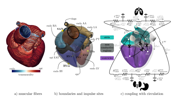
Figure 1: The whole-heart EM model: a) cardiac muscular fibers, (b) boundaries and impulse sites (yellow spheres with bold labels), (c) coupling with circulation and we highlight the three main regions of the EM model (atria, ventricles and non-conductive regions).

The whole-heart EM is based on a comprehensive and biophysically detailed computational model that we recently presented in  [58]. More precisely, we consider a 3D description of cardiac EM in all the four-chambers and a 0D representation of the complete circulatory system, including the cardiac blood hemodynamics [59, 77], as we display in Figure 1c.

The whole-heart EM model includes a detailed myocardial fiber architecture built upon a total-heart Laplace-Dirichlet Rule-Based Method [78], which couples together different methods for the atria [79] and the ventricles [80], to properly reproduce the characteristic features of the cardiac fiber bundles in all the four-chambers [79], see Figure 1a.

Cardiac electrophysiology is described by means of the monodomain equation equipped with no-flux Neumann boundary conditions [81] and endowed with the following human ionic models: ten Tusscher-Panfilov for the ventricles [82] and Courtemanche-Ramirez-Nattel for the atria [83]. Furthermore, the arterial vessels and the atrio-ventricular basal plane are assumed to be non-conductive regions, whence electrically isolating the atria from the ventricles [58]. Finally, the cardiac conduction system is substituted by a series of spherical electrical impulses, originating from the sino-atrial node (SAN) and ending into the left and right ventricular endocardia which, combined with a fast endocardial layer, surrogates the effect of the Purkinje network  [84, 58], as we show in Figure 1b.

The sarcomere mechanical activation is based on the biophysically detailed RDQ20 active contraction model [75], properly calibrated for both atria [85] and ventricles [86]. The RDQ20 is able to represent in detail the sophisticated microscopic active force generation mechanisms, taking place at the scale of sarcomeres [86]. Moreover, to differentiate the active tension in left and right ventricles, we consider a spatially heterogeneous active tension [77].

The myocardial tissue mechanics is described by the momentum balance equation under the hyperelasticity assumption [87]. We employ, for the active part, an orthotropic active stress formulation [77], which surrogates the contraction caused by dispersed myofibers [88], and, for the passive behavior, specific mechanical constitutive laws and model parameters for the different cardiac region: the Usyk constitutive law for both the atria and the ventricles [89] and a Neo-Hookean strain energy density function for the atrio-ventricular basal plane and the vessels [87]. Finally, a nearly incompressible formulation is enforced with a penalty method [58]. Concerning the mechanical boundary conditions, we consider: i) generalized Robin boundary conditions on the epicardium, surrogating both the presence of the pericardium and also the epicardial adipose tissue, crucial for reproducing the correct downward and upward movement of the atrio-ventricular basal plane [58]; ii) normal stress boundary conditions on the four-chamber endocardia and vessel endothelia to account for the pressures exerted by the blood, where the endocardium and endothelium fluid pressures are given by the coupling between the mechanical and the circulation problems [59, 77, 58]; iii) homogeneous Dirichlet boundary condition on all the artificial rings where we cut the computational domain, since the arteries and atrial veins can be considered fixed here [58], as displayed in Figure 1b.

The whole-heart 3D EM model is fully coupled with a 0D closed-loop lumped parameters model for the blood hemodynamics through the entire cardiovascular network. Systemic and pulmonary circulations are modeled using resistance-inductance-capacitance circuits (both for the arterial and venous part) and non-ideal diodes stand for the heart valves  [59]. In Figure 1c we give a graphical representation of the 3D-0D model. The coupling between the 0D and 3D EM models is achieved by introducing volume-consistency coupling conditions, where the pressures of all the four-chambers act as Lagrange multipliers associated with the introduced volume constraints  [59, 77].

The most relevant feedbacks, representing the interactions among electric signal propagation, the cardiac tissue deformation and contraction, and the circulatory system, are modelled inside the whole-heart EM model [58]. These include e.g. the mechano-electric feedback [90] (between electrophysiology and mechanics) and the fibers-stretch and fibers-stretch-rate feedbacks [91] (between mechanics and the activation model).

For the full set of equations of the whole-heart EM model, we refer to [58, 77, 59].

In this paper, the whole-heart EM model serves as unidirectional input for the fluid dynamics problem as we better detail in Section 2.3 and Section 2.4.

2.2 The whole-heart fluid domain

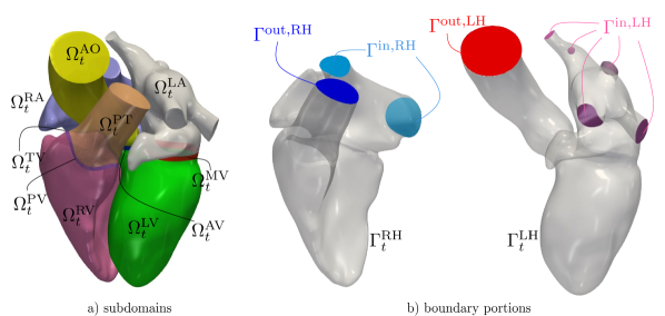
Figure 2: The whole-heart fluid domain: (a) subdomains composing the whole heart; (b) boundary portions (the left and right part are separated for visualization purposes).

Let $\Omega_{t}$ be the fluid domain at time $t>0$ bounded with a sufficiently regular boundary $\Gamma_{t}\equiv\partial\Omega_{t}$ and let $(0,T)$ be the temporal domain, with $T$ the final time. From a fluid dynamics view point, the whole-heart fluid domain $\Omega_{t}$ is topologically disjoint and split into left heart (LH, $\Omega_{t}^{\mathrm{LH}}$) and right heart (RH, $\Omega_{t}^{\mathrm{RH}}$), as we show in Figure 2: $\Omega_{t}=\Omega_{t}^{\text{RH}}\cup\Omega_{t}^{\text{LH}}$, with $\overline{\Omega}_{t}^{\text{RH}}\cap\overline{\Omega}_{t}^{\text{LH}}=\varnothing$. Specifically,

$${\overline{\Omega}_{t}^{\text{RH}}} {=\overline{\Omega}_{t}^{\text{RA}}\cup\overline{\Omega}_{t}^{\text{TV}}\cup\overline{\Omega}_{t}^{\text{RV}}\cup\overline{\Omega}_{t}^{\text{PV}}\cup\overline{\Omega}_{t}^{\text{PT}},}$$

$${\overline{\Omega}_{t}^{\text{LH}}} {=\overline{\Omega}_{t}^{\text{LA}}\cup\overline{\Omega}_{t}^{\text{MV}}\cup\overline{\Omega}_{t}^{\text{LV}}\cup\overline{\Omega}_{t}^{\text{AV}}\cup\overline{\Omega}_{t}^{\text{AO}}},$$

where $\Omega_{t}^{\text{RA}}$, $\Omega_{t}^{\text{RV}}$, $\Omega_{t}^{\text{PT}}$ are the right atrium (RA), right ventricle (RV) and pulmonary trunk (PT) subdomains, and $\Omega_{t}^{\text{LA}}$, $\Omega_{t}^{\text{LV}}$, $\Omega_{t}^{\text{AO}}$ the left atrium (LA), left ventricle (LV) and aorta (AO) subdomains. Moreover, $\Omega_{t}^{\text{TV}}$, $\Omega_{t}^{\text{PV}}$, $\Omega_{t}^{\text{MV}}$, $\Omega_{t}^{\text{AV}}$ are the subdomains representing the rings of the tricuspid valve (TV), pulmonary valve (PV), mitral valve (MV) and aortic valve (AV). Analogously, we partition the boundary of the whole-heart domain as $\Gamma_{t}=\Gamma_{t}^{\text{RH}}\cup\Gamma_{t}^{\text{LH}}$, with $\Gamma_{t}^{\text{RH}}\cap\Gamma_{t}^{\text{LH}}=\varnothing$. In particular, as displayed in Figure 2b,

$$\Gamma_{t}^{\text{RH}}=\Gamma^{\text{out,RH}}\cup\Gamma^{\text{in,RH}}\cup\Gamma_{t}^{\text{w,RH}},$$

with $\Gamma^{\text{in,RH}}$ the inlet sections of the superior and inferior venae cavae, $\Gamma^{\text{out,RH}}$ the outlet section of the pulmonary trunk, and $\Gamma_{t}^{\text{w,RH}}$ the endocardium of the RH. In an analogous fashion, on the left part:

$$\Gamma_{t}^{\text{LH}}=\Gamma^{\text{out,LH}}\cup\Gamma^{\text{in,LH}}\cup\Gamma_{t}^{\text{w,LH}},$$

with $\Gamma^{\text{in,LH}}$ the five inlet sections of the four pulmonary veins, $\Gamma^{\text{out,LH}}$ the outlet section of the aorta, and $\Gamma_{t}^{\text{w,LH}}$ the LH endocardium.

2.3 The fluid domain displacement problem

To represent the deformation of the domain over time, we introduce a fixed reference configuration $\hat{\Omega}\subset\mathbb{R}^{3}$, such that the domain in current configuration $\Omega_{t}$ is defined at any $t\in(0,T)$ as

$$\Omega_{t}=\{\bm{x}\in\mathbb{R}^{3}:\;\bm{x}={\widehat{\bm{x}}}+\bm{d}({\widehat{\bm{x}}},t),\;{\widehat{\bm{x}}}\in\widehat{\Omega}\},$$

where $\bm{d}:\widehat{\Omega}\times(0,T)$ is the displacement of the domain, and is obtained it by solving the following harmonic extension problem:

$$-\divergence(s\gradient\bm{d})=\mathbf{0} \widehat{\Omega}\times(0,T),$$ in (1a)

$$\bm{d}=\bm{d}^{\partial\Omega}(\mathbf{x},t) {\partial\widehat{\Omega}}\times(0,T)$$ on . (1b)

In Equation 1b, $\bm{d}^{\partial\Omega}:{\partial\widehat{\Omega}}\times(0,T)$ is the boundary displacement, computed by restricting the solution of the EM simulation to the endocardium and the endothelium. Furthermore, $s:{\widehat{\Omega}}\times(0,T)\to\mathbb{R}$ is a space-dependent scalar field introduced to avoid distortion of mesh elements. Specifically, we use the boundary-based stiffening approach proposed in [92]. We denote the fluid domain displacement problem Equation 1b with the abridged notation

$${\mathscr{D}}(\bm{d},\bm{d}^{\partial\Omega})=0.$$

The EM simulation is solved with a significantly larger timestep than the CFD one. Therefore, the boundary displacement $\bm{d}^{\partial\Omega}$ is only available for some times $t_{k}$, $k=0,1,\dots,N_{\text{EM}}$, although the domain displacement $\bm{d}$ is needed with a finer temporal resolution. Thus, problem (1b) is solved for all times $t_{k}$, and then we construct a displacement field $\tilde{\bm{d}}(t):\widehat{\Omega}\times(0,T)\to\mathbb{R}^{3}$ using smoothing splines approximation in time  [93].

We compute the domain velocity by deriving the displacement in time as

$$\bm{u}^{\mathrm{ALE}}=\partialderivative{\widetilde{\bm{d}}}{t}\;\;\mathrm{in}\;\Omega_{t}\times(0,T).$$ (2)

2.4 The Navier-Stokes equations in ALE framework with the RIIS model of the valves

We model the blood in the cardiac cavities as an incompressible, viscous and Newtonian fluid characterized by constant density $\rho$ and constant dynamic viscosity $\mu$. We therefore use the time-dependent incompressible Navier-Stokes equations expressed in an Arbitrary Lagrangian Eulerian (ALE) framework to account for the moving domain. We denote by $\bm{u}:\Omega_{t}\times(0,T)\to\mathbb{R}^{3}$ and $p:\Omega_{t}\times(0,T)\to\mathbb{R}$ the fluid velocity and pressure, respectively. Let $\sigma$ be the Cauchy stress tensor, defined for incompressible, Newtonian and viscous fluids as $\sigma(\bm{u},p)=-pI+2\mu\epsilon(\bm{u})$, with $\epsilon(\bm{u})=\frac{1}{2}\left(\gradient\bm{u}+(\gradient\bm{u})^{T}\right)$ the strain-rate tensor.

We model the effects of cardiac valves in the fluid by means of the Resistive Immersed Implicit Surface (RIIS) method [71]. We consider four immersed surfaces ${\Sigma_{\mathrm{k}}}$, with ${\mathrm{k}}\in\mathcal{I}_{\mathrm{v}}=\left\{\text{MV, AV, TV, PV}\right\}$ the set of valves. Each valve is characterized by a resistance coefficient $R_{\mathrm{k}}$ and a parameter $\varepsilon_{\mathrm{k}}$ representing the half thickness of the valve leaflets. The immersed surface is implicitly described by a signed distance function $\varphi_{\mathrm{k}}:\Omega_{t}\times(0,T)\to\mathbb{R}$. With the RIIS method, we introduce the following penalty term to the momentum balance of the Navier-Stokes equations (expressed in ALE form):

$$\bm{\mathcal{R}}(\bm{u},\bm{u}^{\mathrm{ALE}})=\sum_{{\mathrm{k}}\in\mathcal{I}_{\mathrm{v}}}\frac{R_{\mathrm{k}}}{\varepsilon_{\mathrm{k}}}\delta_{{\Sigma_{\mathrm{k}}},\varepsilon_{\mathrm{k}}}(\varphi_{\mathrm{k}})\left(\bm{u}-\bm{u}^{\mathrm{ALE}}-\bm{u}_{{\Sigma_{\mathrm{k}}}}\right).$$

$\bm{\mathcal{R}}$ penalizes the mismatch between the relative velocity $\bm{u}-\bm{u}^{\mathrm{ALE}}$ and the velocity of the valves’ leaflets $\bm{u}_{{\Sigma_{\mathrm{k}}}}$, weakly imposing a kinematic coupling condition only. The resistive term is only acting on a tiny support around ${\Sigma_{\mathrm{k}}}$, thanks to a smoothed Dirac delta function acting as multiplicative factor. We refer to [71] for its definition.

By defining with $\frac{\widehat{\partial}\bm{u}}{\partial t}=\partialderivative{\bm{u}}{t}+(\bm{u}^{\mathrm{ALE}}\cdot\nabla)\bm{u}$ the ALE derivative, the 3D fluid dynamics model of the whole heart reads:

$$\rho\frac{\widehat{\partial}\bm{u}}{\partial t}+((\bm{u}-\bm{u}^{\mathrm{ALE}})\cdot\gradient)\bm{u}+\divergence\sigma(\bm{u},p)+\bm{\mathcal{R}}(\bm{u},\bm{u}^{\mathrm{ALE}})=\bm{0} \Omega_{t}\times(0,T)$$ in , (3a)

$$\divergence\bm{u}=0 \Omega_{t}\times(0,T)$$ in , (3b)

$$\sigma(\bm{u},p)\bm{n}=-p^{\mathrm{in}}_{\mathrm{RA}}\bm{n} \Gamma^{\mathrm{in,RH}}\times(0,T)$$ on , (3c)

$$\sigma(\bm{u},p)\bm{n}=-p^{\mathrm{PUL}}_{\mathrm{AR}}\bm{n} \Gamma^{\mathrm{out,RH}}\times(0,T),$$ on (3d)

$$\sigma(\bm{u},p)\bm{n}=-p^{\mathrm{in}}_{\mathrm{LA}}\bm{n} \Gamma^{\mathrm{in,LH}}\times(0,T),$$ on (3e)

$$\sigma(\bm{u},p)\bm{n}=-p^{\mathrm{SYS}}_{\mathrm{AR}}\bm{n} \Gamma^{\mathrm{out,LH}}\times(0,T),$$ on (3f)

$$\bm{u}=\bm{u}^{\mathrm{ALE}} \Gamma_{t}^{\text{w,RH}}\cup\Gamma_{t}^{\text{w,LH}}\times(0,T).$$ on (3g)

$$\bm{u}=\bm{u}_{0} \Omega_{0}\times\{0\}$$ in , (3h)

where $p^{\mathrm{in}}_{\mathrm{RA}},\,p^{\mathrm{PUL}}_{\mathrm{AR}},\,p^{\mathrm{in}}_{\mathrm{LA}},\,p^{\mathrm{SYS}}_{\mathrm{AR}}$ are the pressures arising from the coupling with the circulation model, as we detail in Section 2.5, and $\bm{u}_{0}$ is the initial velocity. We denote the 3D fluid dynamics model of the whole heart in Equation 3h by

$$\mathscr{F}(\bm{u},p,\bm{u}^{\mathrm{ALE}})=0.$$

2.5 Coupling with circulation

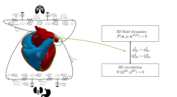
Figure 3: The 3D-0D fluid dynamics model of the whole-heart coupled to the surrounding circulation.

To account for the interplay between the heart’s fluid dynamics and the hemodynamics of the surrounding circulation, we couple the cardiac CFD model to a 0D closed-loop model of the whole circulation proposed in [59]. Specifically, we extend to the whole heart the coupling strategy that we devised in [26] for the case of the sole left heart. We consider a reduced (open) version of the original circulation model in which we remove the equations for all the variables that are already described by the 3D counterpart. The equations of the open system are reported in A. By denoting with $\bm{Q}^{\mathrm{0D}}$ and $\bm{p}^{\mathrm{0D}}$ the vectors containing flowrates and pressures of the 0D model, respectively, we refer to the open system with the notation

$$\mathscr{C}(\bm{Q}^{\mathrm{0D}},\bm{p}^{\mathrm{0D}})=0.$$

The coupling between the 3D CFD model and the open 0D model consists in the enforcement of the continuity of pressures and flowrates on the artificially chopped boundaries $\Gamma^{\mathcal{I}}$ of the fluid domain, yielding the following conditions:

$$p^{\mathcal{I}}_{\mathrm{3D}}=p^{\mathcal{I}}_{\mathrm{0D}} \text{ on }\Gamma^{\mathcal{I}}\times(0,T),$$ (4a)

$$Q^{\mathcal{I}}_{\mathrm{3D}}=Q^{\mathcal{I}}_{\mathrm{0D}} \text{ on }\Gamma^{\mathcal{I}}\times(0,T),$$ (4b)

which express dynamic and kinematic coupling, respectively, with

$$p^{\mathcal{I}}_{\mathrm{3D}}=\frac{1}{|\Gamma^{\mathcal{I}}|}\int_{\Gamma^{\mathcal{I}}}p,\qquad Q^{\mathcal{I}}_{\mathrm{3D}}=\int_{\Gamma^{\mathcal{I}}}(\bm{u}-\bm{u}^{\mathrm{ALE}})\cdot\bm{n}.$$ (5)

Considering the whole-heart fluid domain (see Figure 2b), the interface boundaries are $\Gamma^{\mathcal{I}}=\Gamma^{\mathrm{in,RH}}\cup\Gamma^{\mathrm{out,RH}}\cup\Gamma^{\mathrm{in,LH}}\cup\Gamma^{\mathrm{out,LH}}$. The 0D pressures ($p^{\mathcal{I}}_{\mathrm{0D}}$) and flowrates ($p^{\mathcal{I}}_{\mathrm{0D}}$) are [42, 94]:

$$p^{\text{in,RH}}_{\mathrm{0D}}=p_{\mathrm{RA}}^{\mathrm{in}}, Q^{\text{in,RH}}_{\mathrm{0D}}=-Q^{\mathrm{SYS}}_{\mathrm{VEN}},$$

$$p^{\text{out,RH}}_{\mathrm{0D}}=p^{\mathrm{PUL}}_{\mathrm{AR}}+R^{\mathrm{PUL}}_{\mathrm{upstream}}Q_{\mathrm{PV}}, Q^{\text{out,RH}}_{\mathrm{0D}}=Q_{\mathrm{PV}},$$

$$p^{\text{in,LH}}_{\mathrm{0D}}=p^{\mathrm{in}}_{\mathrm{LA}}, Q^{\text{in,LH}}_{\mathrm{0D}}=-Q^{\mathrm{PUL}}_{\mathrm{VEN}},$$

$$p^{\text{out,LH}}_{\mathrm{0D}}=p^{\mathrm{SYS}}_{\mathrm{AR}}+R^{\mathrm{SYS}}_{\mathrm{upstream}}Q_{\mathrm{AV}}, Q^{\text{out,LH}}_{\mathrm{0D}}=Q_{\mathrm{AV}}.$$

From the point of view of the 3D CFD model, the conditions expressed by Equation 5 are defective, since they prescribe the average pressure and the total flow rate over the entire section $\Gamma^{\mathcal{I}}$, rather than pointwise stress and velocity distributions [50]. We choose to complete the pressure condition as

$$\sigma(\bm{u},p)\bm{n}=-p^{\mathcal{I}}\bm{n},\text{ on }\Gamma^{\mathcal{I}}\times(0,T).$$ (6)

The flowrate condition, conversely, is left in its defective form, since it is sufficient for the algorithm we use for the 3D-0D coupling (see Section 3).

3 Numerical methods

Algorithm 1 Numerical scheme for the EM-driven CFD simulation of the whole heart

  Solve whole-heart EM model

  Pick solution in the last heartbeat: $\to\bm{d}^{\mathrm{EM}}_{i}$, for $i=0,\dots,N$

  Restrict $\bm{d}^{\mathrm{EM}}_{i}$ on $\partial\Omega_{i}^{\mathrm{S},\mathrm{endo}}$: $\bm{d}^{\partial\Omega}_{i},\text{ for }i=0,\dots,N$

  Solve fluid domain displacement problem: ${\mathscr{D}}(\bm{d}_{i},\bm{d}^{\partial\Omega}_{i})=0,\text{ for }i=0,\dots,N$

  Build approximant: $\widetilde{\bm{d}}(t)$

  Initialization: $n=0,\,\bm{u}_{0}=\bm{0}$

  while $n<N_{t}$ do

      Update valves leaflet position Compute ALE velocity: $\bm{u}^{\mathrm{ALE}}_{n+1}=\frac{\widetilde{\bm{d}}_{n+1}-\widetilde{\bm{d}}_{n}}{\Delta t}$. Solve circulation: $\mathscr{C}(\bm{Q}^{\mathrm{0D}}_{n+1},\bm{p}^{\mathrm{0D}}_{n+1})=0$ with data $Q^{\mathcal{I}}_{\mathrm{0D},n}$ Compute interface data (0D $\to$ 3D): $p^{\mathcal{I}}_{\mathrm{0D},n+1}\to p^{\mathcal{I}}_{\mathrm{3D},n+1}$ Solve fluid dynamics: $\mathscr{F}(\bm{u}_{n+1},p_{n+1},\bm{u}^{\mathrm{ALE}}_{n+1})=0$, with Neumann data $p^{\mathcal{I}}_{\mathrm{3D},n+1}$ Compute interface data (3D $\to$ 0D): $Q^{\mathcal{I}}_{\mathrm{3D},n+1}\to Q^{\mathcal{I}}_{\mathrm{0D},n+1}$ $n\leftarrow n+1.$

  end while

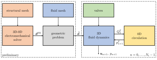
Figure 4: Graphical representation of the overall algorithm to simulate the whole-heart hemodynamics driven by the EM model.

In this section, we describe the numerical methods we use to solve our multiphysics and multiscale system. The overall algorithm is presented in Algorithm 1 and graphically represented in Figure 4. We can subdivide the overall procedure in a preliminary phase, in which we solve the EM simulation [58] and the fluid domain displacement problem to lift the boundary displacement to the fluid bulk domain, followed by the coupled 3D-0D CFD simulation.

Numerical methods for the EM model

For the numerical approximation of the whole-heart EM model we employ the efficient Segregated-Staggered scheme [59, 77, 58]. In this numerical scheme, the different cardiac physical models, contributing to both the 3D EM and the 0D blood circulation, are sequentially solved in a segregated manner, using different resolutions in space and time to properly account for the heterogeneous space and time scales characterizing different physical processes [95].

For the space discretization, we use the Finite Element (FE) method with continuous FE on a tetrahedral mesh. We consider FE of order 2 ($\mathbb{P}_{2}$) for the electrophysiology to capture the traveling wave dynamics and FE of order 1 ($\mathbb{P}_{1}$) for both the activation and the mechanics [58].

For the time discretization, we use finite difference schemes [96]. Specifically, cardiac electrophysiology is solved with Backward Differentiation Formula (BDF) of order 2, using an Implicit-Explicit (IMEX) scheme where the diffusion term is treated implicitly, the ionic and reaction terms explicitly. The ionic variables are advanced in time through an IMEX scheme [59, 77, 58]. We solve the active contraction problem with an IMEX BDF1 method, and the mechanical problem with a fully-implicit BDF1 scheme [77]. Finally, an IMEX scheme of the first order is used for the circulation [58]. Moreover, two different time steps are used: a finer one for the electrophysiology and a larger one for both the activation, the mechanics and the circulation [59]. Finally, we employ recently developed stabilization methods – related to the circulation and the fibers-stretch-rate feedback – that are crucial to obtain a stable solution in a four-chamber simulation scenario [97, 98]. Concerning the linear systems arising from the discretization of the whole-heart EM problem we use: the conjugate gradient for the electrophysiology and the GMRES method for both the mechanics and the activation, both empowered by an algebraic multigrid (AMG) preconditioner. Finally, we solve the non-linear saddle-point problem arising from the coupling between the mechanics and the circulation by means of a Newton algorithm using, at the algebraic level, the Schur complement reduction  [77, 59].

For further details about the numerical methods we use in the whole-heart EM model, we refer to [59, 77, 58].

Numerical methods for the fluid domain displacement problem

After simulating the whole-heart EM and reaching a limit cycle in terms of pressure and volumes, we extract the solution from the last simulated heartbeat. We restrict this solution to the heart endocardium and the endothelium of outflow tracts, obtaining $N+1$ solutions defined on the boundary of the fluid domain ($\bm{d}^{\partial\Omega}_{i}$, with $i=0,\dots,N$). We project $\bm{d}^{\partial\Omega}_{i}$ onto the CFD mesh with piecewise linear interpolation, then solve the fluid domain displacement problem in Equation 1b to obtain the ALE displacement $\bm{d}$. We discretize the lifting problem in Equation 1b using FEs of order 1 ($\mathbb{P}_{1}$) and the linear system arising from its discretization is preconditioned with an AMG preconditioner. We solve the resulting linear system with the conjugate gradient method. The smoothing spline approximation is computed independently for each mesh node, and the approximant is constructed following the optimization procedure described in [99]. To compute the ALE velocity, we use BDF1 to discretize in time Equation 2.

Numerical methods for the CFD cardiac model

We discretize Equation 3h in space using FEs of order 1 for both velocity and pressure ($\mathbb{P}_{1}-\mathbb{P}_{1}$). We employ the Variational Multiscale - Large Eddy Simulation (VMS-LES) method to obtain a stable formulation of the NS-ALE-RIIS equations discretized via equal order FE spaces. This also allows us to control instabilities arising from the advection-dominated regime, and to model transition-to-turbulence in the LES framework [100, 101, 16]. The VMS-LES formulation accounts for the ALE framework and the RIIS modeling used for valves. For the complete formulation, we refer to [26].

For the time discretization, we consider a uniform partition of the temporal domain in $N_{t}$ subintervals $(t_{n},t_{n+1}]$ of uniform size $\Delta t$, with $n=0,\dots,N_{t}-1$. We denote from here quantities approximated at time $t_{n}$ with the subscript $n$, e.g. $\bm{u}_{n}\approx\bm{u}(t_{n})$. We advance the problem in time by means of BDF1. To reduce the computational burden of the numerical simulations, we use a semi-implicit treatment of the nonlinearities, as done in [100]. The overall numerical scheme for the fluid dynamics problem is detailed in [26].

Since Neumann boundary conditions may give rise to instability phenomena in case of inflow, we set backflow stabilization on all the Neumann boundaries in the inertial form presented in [102].

The linear system arising from the discretization of Equation 3h is preconditioned with the aSIMPLE preconditioner [103], and each of its blocks is preconditioned with an AMG preconditioner. The linear system is then solved at each time step by the GMRES method.

Numerical method for the 0D circulation model

We solve the system of ODEs of the circulation problem with an IMEX method of the first order. The time-step size $\Delta t$ employed for its numerical discretization is the same used for the BDF advancing scheme in the 3D problem.

Numerical scheme for the coupled CFD problem

After initialization, for each temporal step of the CFD problem, we update the position of valve leaflets and we compute the ALE velocity. At every time step, we solve the 3D and 0D subproblems independently. First, we solve the 0D open circulation problem using $Q^{\mathcal{I}}_{n}$ as input (i.e. the flowrates computed in the 3D model at previous timestep, namely $Q^{\mathrm{SYS}}_{\mathrm{VEN},n},\,Q_{\mathrm{PV},n},\,Q^{\mathrm{PUL}}_{\mathrm{VEN},n},\,Q_{\mathrm{AV},n}$). Then, from the solution of the circulation, we compute the pressures $p^{\mathcal{I}}_{n+1}$ at the interfaces and solve the fluid dynamics problem providing those pressures as Neumann boundary conditions at inlet and outlet sections. Finally, we compute the interface data from the 3D to the 0D model, i.e. $Q^{\mathcal{I}}_{n+1}$. This approach treats the coupling between the 3D and 0D subproblems in a segregated and explicit way.

4 Numerical results

In this section, we present the numerical results using the whole-heart fluid dynamics model. In Section 4.1, we introduce the computational setting of the whole-heart EM and CFD simulations. Section 4.2 is devoted to the calibration of the RDQ20 activation model to produce physiological flowrates in the EM simulation. The physiological results of the overall computational model are presented in Section 4.3. Finally, we apply the multiphysics computational model to the pathological case of LBBB in Section 4.4.

4.1 Computational setup

We consider a realistic whole-heart geometry provided by the Zygote solid 3D heart model [104], an anatomically CAD model representing an average healthy human heart reconstructed from high-resolution computer tomography scan data. We generate whole-heart tetrahedral meshes for the EM and CFD problems that we report in Figure 5. Meshes are generated with vmtk [105] using the methods and tools discussed in [106, 58, 26]. Details on the meshes for the EM and CFD simulations are provided in Table 1. The valve leaflets are thin structures that we characterize, in the context of the RIIS method, by small values of $\varepsilon_{\mathrm{k}}$. To correctly capture the immersed surfaces, we refine the CFD mesh close to the valve regions, as shown in Figure 5c. Specifically, following [71], we choose $h_{\text{k}}$ such that $\varepsilon_{\mathrm{k}}\geq 1.5h_{\text{k}}$, where $h_{\text{k}}$ is the minimum mesh size of the fluid mesh in the valve region.

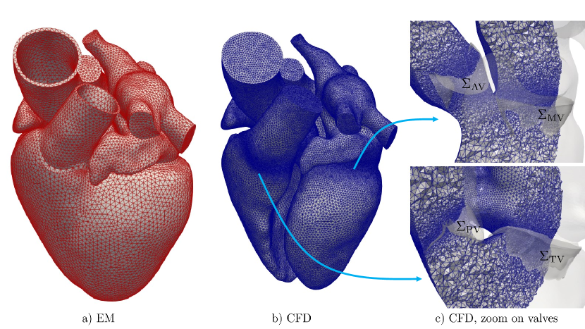
Figure 5: Tetrahedral meshes used in the computational model: a) mesh for the EM simulation, b) mesh for the CFD simulation, c) mesh refinement on the valves region of the CFD mesh.

Simulation	Mesh size [$\mathrm{mm}\text{/}$]			Cells	Points	Physics	DOFs	$\Delta t$ [$\mathrm{s}\text{/}$]
	min	avg	max
EM	$0.860$	$2.97$	$5.34$	$180\,472$	$46\,915$	Electrophysiology	$310\,505$	$5\text{⋅}{10}^{-5}$
						Mechanics	$140\,745$	$10^{-3}$
						Circulation	-	$10^{-3}$
CFD	$0.210$	$1.04$	$3.82$	$3\,892\,584$	$652\,204$	Fluid dynamics	$2\,608\,816$	$10^{-4}$
						Circulation	-	$10^{-4}$

Table 1: Setup of whole-heart EM and CFD simulations (mesh details and time step sizes).

We carry out EM and CFD simulations in life${}^{\texttt{x}}$ [107, 108], a high-performance C++ FE library developed within the iHEART project, mainly focused on cardiac simulations and based on the deal.II finite element core [109, 110, 111].

Numerical simulations are run in parallel on the GALILEO100 supercomputer at the CINECA supercomputing center, using 240 and 480 cores for the EM and CFD simulations, respectively. The computational time to carry out a single heartbeat is about 1 hour and 20 minutes for the EM simulation and 56 hours for the CFD simulation.

For the parameters of the EM model, we use the same values as in [58] with some minor differences reported in B. As we better discuss in Section 4.2, a huge difference in terms of setup of the EM simulation between [58] and the present work consists in the calibration of the activation model to compute physiological blood flowrates. We simulate 20 heartbeats of the whole-heart EM, and we report numerical results related to the last heartbeat, after verifying that the solution is sufficiently close to a periodic limit cycle (in terms of pressure and volume transients). We consider an heartbeat period of $T_{\mathrm{HB}}=$0.8$\,$\mathrm{s}\text{/}$$. We pick the last simulated EM heartbeat as input displacement for the CFD simulation. We set as initial condition for the velocity $\bm{u}_{0}=\bm{0}$. The initial state of the circulation model (for the coupling with the fluid dynamics) is taken equal to the values reached at the beginning of the last heartbeat in the EM simulation. Moreover, as detailed in B, all the values of the parameters involved in the circulation model are the same for the EM and the fluid dynamics simulations. The physical parameters for blood are density $\rho=$1.06\text{⋅}{10}^{3}\text{\,}\mathrm{kg}\text{/}{\mathrm{m}}^{3}$$ and dynamic viscosity $\mu=$3.5\text{⋅}{10}^{-3}\text{\,}\mathrm{kg}\text{/}\text{(}\mathrm{m}\text{\,}\mathrm{s}\text{)}$$. We simulate two heart cycles, and we report the solution on the second cycle to remove the consequences of an unphysical null initial condition. For the numerical results visualization (for both EM and CFD), we shift the time domain in $(0,T_{\mathrm{HB}})$.

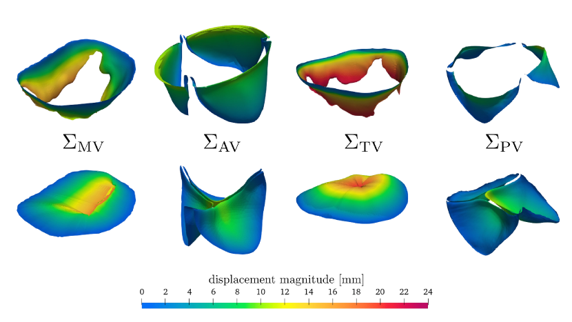
Figure 6: Cardiac valves in their open and closed configurations coloured according to displacement magnitude. Valves geometry are provided by Zygote [104], and we define displacement field aimed at closing and opening the leaflets.

The Zygote cardiac valves [104] are provided in their open configuration (TV, MV) and closed configuration (PV, AV). Thus, we define displacement fields aimed at closing and opening their leaflets, based on signed-distance functions and the solution of Laplace-Beltrami problems [106, 26]. In Figure 6, we report the valves in their open and closed configurations, colored according to the leaflets’ displacement magnitude. We open and close the valves instantaneously (i.e. in one time step) at the times reported in Table 2. These times are chosen by selecting the initial and final times of the isovolumetric phases. The values we choose for $\varepsilon_{\mathrm{k}}$, reported in Table 2, allow to have a physiological representation of the valve leaflet. Indeed, we choose $\varepsilon_{\mathrm{k}}$ by averaging the values of the leaflet thicknesses reported in [112]. Furthermore, the valve resistances values $R_{\mathrm{k}}$ are reported in Table 2. We found that the condition number of the linear system associated to the FE discretization of the fluid dynamics problem becomes larger as the ratio $R_{\mathrm{k}}/\varepsilon_{\mathrm{k}}$ increases. Thus, to keep contained the computational cost of the CFD simulation, we choose as $R_{\mathrm{k}}$ the minimum value that guarantees impervious valves.

		MV	AV	TV	PV
opening time	[$\mathrm{s}\text{/}$]	$0.710$	$0.262$	$0.700$	$0.279$
closing time	[$\mathrm{s}\text{/}$]	$0.208$	$0.666$	$0.194$	$0.677$
$R_{\mathrm{k}}$	[$\mathrm{k}\mathrm{g}\mathrm{/}{\mathrm{m}\mathrm{/}\mathrm{s}}$]	$10^{4}$	$10^{4}$	$10^{4}$	$10^{4}$
$\varepsilon_{\mathrm{k}}$	[$\mathrm{mm}\text{/}$]	$0.68$	$0.67$	$0.77$	$0.52$

Table 2: Setup of the RIIS method to model cardiac valves.

4.2 Calibration of the RDQ20 activation model to achieve physiological flows

Among the different components at the basis of cardiac EM simulations, the model describing the active force generation at the microscale plays a pivotal role on the solution. Indeed, not only the amount of force the muscle develops depends on it, but also its temporal distribution over the heartbeat, i.e., the kinetics of contraction and relaxation. Muscle contraction, in turn, determines the blood flow through the valves. Moreover, since the electromechanical displacement drives the fluid dynamics model, the same flows are then obtained in the CFD simulation. Therefore, special care must be devoted here to the choice and calibration of the activation model, in order to faithfully capture blood flowrates and, consequently, blood velocities.

For the above reasons, we chose to use the RDQ20 model [75], that is an active force model with high biophysical fidelity and that is able to reproduce the main features of the experimentally observed behaviors. The RDQ20 model is based on a detailed description of the calcium-driven regulation of the thin filament, with explicit representation of end-to-end cooperative interactions, and a description of the attachment-detachment process of crossbridges, at the basis of the force-velocity relationship. Thereby, the model is able to reproduce the main mechanisms of contractility regulation, mediated by calcium, fiber strain and fiber strain-rate. In particular, the fiber strain-rate feedback, which is responsible for the well-known force-velocity relationship, plays a central role in the regulation of hemodynamic flows, as demonstrated in [58] and confirmed in the present study.

On this basis, we refine the calibration of the RDQ20 model, with a particular care on fluxes through semilunar valves obtained by means of the 0D model in the EM simulation. We employ as a starting point the calibration used in [58], suitable for the coupling with the TTP06 ionic model [82] (see Table 3, setting A). In Table 4, column A, we report a list of biomarkers obtained by using the calibration A in the EM simulation. Although the biomarkers characterizing the overall cardiac function (i.e. end-systolic and end-diastolic volume, stroke volume and ejection fraction) are within reference ranges, the maximum blood flux across valves is significantly above the physiological range. In other terms, even if the total ejected blood is physiological, the instantaneous flow peak is too large. This would clearly have a strong negative impact on the results of fluid dynamics simulations. For instance, an excessively high velocity through the valve may result in high pressure gradients, and an overall incorrect stress distribution over valve leaflets and cardiac walls [113, 114].

Parameter		A	B	C	D	E
Regulatory units dynamics
$Q$	[$\mathrm{-}$]	2	2	2	2	2
$\overline{k}_{\mathrm{d}}$	[$\mathrm{\SIUnitSymbolMicro M}\text{/}$]	0.36	0.36	0.36	0.36	0.36
$\alpha_{k_{\mathrm{d}}}$	[$\mathrm{\SIUnitSymbolMicro M}\text{/}\mathrm{\SIUnitSymbolMicro m}$]	-0.2083	-0.2083	-0.2083	-0.2083	-0.2083
$\mu$	[$\mathrm{-}$]	10	10	10	10	10
$\gamma$	[$\mathrm{-}$]	30	30	30	30	30
$K_{\mathrm{off}}$	[$\text{/}\mathrm{s}$]	8	(*)4	(*)4	(*)4	(*)4
$K_{\mathrm{basic}}$	[$\text{/}\mathrm{s}$]	4	(*)2	(*)2	(*)2	(*)2
Crossbridge dynamics (prescribed)
$v_{0}$	[$\text{/}\mathrm{s}$]	2	2	2	2	(*)0.5
$v_{\mathrm{max}}$	[$\text{/}\mathrm{s}$]	8	8	8	8	(*)2
$\tilde{k}_{2}$	[$\mathrm{-}$]	66	66	66	66	66
$\mu_{0}^{\text{iso}}$	[$\mathrm{-}$]	0.22	0.22	0.22	0.22	0.22
Crossbridge dynamics (automatically calibrated)
$r_{0}$	[$\text{/}\mathrm{s}$]	134.31	134.31	134.31	134.31	33.24
$\alpha$	[$\mathrm{-}$]	25.184	25.184	25.184	25.184	24.93
$\mu^{0}_{f_{\mathcal{P}}}$	[$\text{/}\mathrm{s}$]	32.225	32.225	32.225	32.225	7.98
$\mu^{1}_{f_{\mathcal{P}}}$	[$\text{/}\mathrm{s}$]	0.768	0.768	0.768	0.768	0.192
Micro-macro upscaling
$a_{\mathrm{XB}}$	[$\mathrm{MPa}\text{/}$]	1500.0	(*)1550.0	(*)2925.0	(*)5214.5	(*)1550.0

Table 3: Different calibrations of the RDQ20 activation model: A) calibration from [58]; B) C) D) Reduced $K_{\mathrm{off}},\,K_{\mathrm{basic}}$ and different levels of $a_{\mathrm{XB}}$; E) Reduced $v_{0},\,v_{\mathrm{max}}$. Parameters that are modified with respect to A are highlighted by the symbol (*). We remark that the parameters $r_{0}$, $\alpha$, $\mu^{0}_{f_{\mathcal{P}}}$ and $\mu^{1}_{f_{\mathcal{P}}}$ are automatically calibrated from the four quantities $v_{0}$, $v_{\mathrm{max}}$, $\tilde{k}_{2}$ and $\mu_{0}^{\text{iso}}$ (for furhter details, see [75]); therefore, the symbol (*) is not reported for these four parameters. For the description of each parameter, we refer to the original paper of the RDQ20 model [75].

Biomarker		Physiological values		A	B	C	D	E
$\mathrm{ESV}_{\mathrm{LV}}$	[$\mathrm{ml}\text{/}$]	35 to 80	[115]	53.8	66.7	53.5	45.9	66.4
$\mathrm{ESV}_{\mathrm{RV}}$	[$\mathrm{ml}\text{/}$]	69 $\pm$ 22	[116]	58.0	79.8	65.3	56.0	72.3
$\mathrm{EDV}_{\mathrm{LV}}$	[$\mathrm{ml}\text{/}$]	126 to 208	[115]	150	128	($\downarrow$)108	($\downarrow$)87.9	151
$\mathrm{EDV}_{\mathrm{RV}}$	[$\mathrm{ml}\text{/}$]	144 $\pm$ 23	[117]	153	152	134	119	159
$\mathrm{SV}_{\mathrm{LV}}$	[$\mathrm{ml}\text{/}$]	81 to 137	[115]	96.3	($\downarrow$)61.5	($\downarrow$)54.9	($\downarrow$)42.0	84.9
$\mathrm{SV}_{\mathrm{RV}}$	[$\mathrm{ml}\text{/}$]	94 $\pm$ 15	[117]	95.4	($\downarrow$)72.3	($\downarrow$)69.1	($\downarrow$)63.2	87.1
$\mathrm{EF}_{\mathrm{LV}}$	[%]	49 to 73	[118]	64.2	($\downarrow$)48.0	50.2	($\downarrow$)47.8	56.1
$\mathrm{EF}_{\mathrm{RV}}$	[%]	53 $\pm$ 6	[119]	($\uparrow$)62.2	47.5	51.4	53.0	54.6
$\mathrm{Q}_{\mathrm{AV}}^{\mathrm{max}}$	[$\mathrm{ml}\text{/}\mathrm{s}$]	427 $\pm$ 129	[120]	($\uparrow$)697	327	347	304	399
$\mathrm{Q}_{\mathrm{PV}}^{\mathrm{max}}$	[$\mathrm{ml}\text{/}\mathrm{s}$]	427 $\pm$ 129	[120]$\dagger$	($\uparrow$)756	397	427	443	478
$\mathrm{p}_{\mathrm{LV}}^{\mathrm{max}}$	[$\mathrm{mmHg}\text{/}$]	119 $\pm$ 13	[121]	($\uparrow$)154	($\downarrow$)99.5	($\downarrow$)93.2	($\downarrow$)80.7	120
$\mathrm{p}_{\mathrm{RV}}^{\mathrm{max}}$	[$\mathrm{mmHg}\text{/}$]	35 $\pm$ 11	[122]	37.2	34.9	38.2	41.6	32.2

Table 4: Effects of different calibrations of the RDQ20 activation model on mechanics and hemodynamics biomarkers. Biomarkers highlighted by the symbols ($\uparrow$) and ($\downarrow$) lie outside the reference ranges, denoting values too large or too small, respectively, compared with reference ranges. $\dagger$: for the maximum PV flowrate, in absence of clinical ranges from literature, we consider the same normal values of the AV flowrate. Each column corresponds to a different calibration as detailed in Table 3.

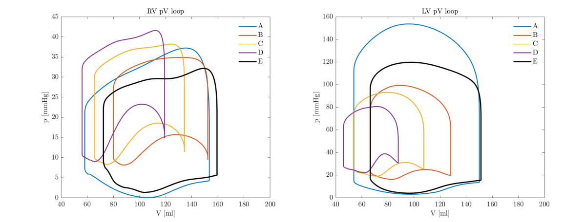
Figure 7: pV loops of RV and LV obtained with different calibrations of the RDQ20 activation model. Each line corresponds to a different calibration as detailed in Table 3.

To address this issue, we slow down the process of force generation, so that the tissue contractility is developed at a lower rate. More precisely, we reduce the association-dissociation rates of troponin and tropomyosin of the RDQ20 model (i.e. $K_{\mathrm{off}}$ and $K_{\mathrm{basic}}$) by a factor 2. Moreover, to compensate for the lower peak force caused by a slower kinetics, we increase the crossbridge level contractility (i.e. $a_{\mathrm{XB}}$). We consider three different levels of contractility, as reported in Table 3, respectively in columns B, C and D. However, as we show in Table 4 and Figure 7, on the one hand, we achieve the desired effect of reducing semilunar peak flows, thus bringing them within the expected ranges. On the other hand, we compute significantly reduced stroke volume and ejection fraction for both chambers, thus moving out of physiological ranges. Notice also that this issue is also not resolved by adjusting the contractility. In fact, by raising $a_{\mathrm{XB}}$, not only the state of contractility in systole is changed, but also in diastole, leading to a reduced end-diastolic volume and, therefore, nullifying the effect of increased contractility, due to the Frank-Starling mechanism. The three cases shown in Table 4 (B, C and D) are three illustrative cases out of the many that we tested, but without being able to reduce peak flows within the expected ranges while maintaining a physiological ejection fraction. The tests evidenced a paradigmatic short-blanket problem, whereby just acting on kinetics and contractility it is not possible to lower the flows while maintaining a regular ejection fraction. Evidently, another element must be taken into account.

Based on the results of [58], which showed that, by neglecting the fibers-stretch-rate feedback, blood flows through the semilunar valves are significantly overestimated, we modified the calibration so as to, on the contrary, strengthen the effect of this feedback, but without changing either the isometric force or the kinetics. Specifically, we acted in such a way as to steepen the force-velocity relationship, the microscopic mechanism underlying the fibers-stretch-rate feedback, by modifying the parameters governing cross-bridge dynamics. For this purpose, we took advantage of the calibration technique illustrated in [75], by which the RDQ20 model can be tuned to achieve a desired force-velocity relationship. Two features of the force-velocity relationship can be selected, namely the maximum shortening velocity ($v_{\mathrm{max}}$), that is the velocity corresponding to vanishing active force, and the tangent to the curve under isometric conditions ($v_{0}$). The geometric meaning of the two quantities is illustrated in Figure 8.

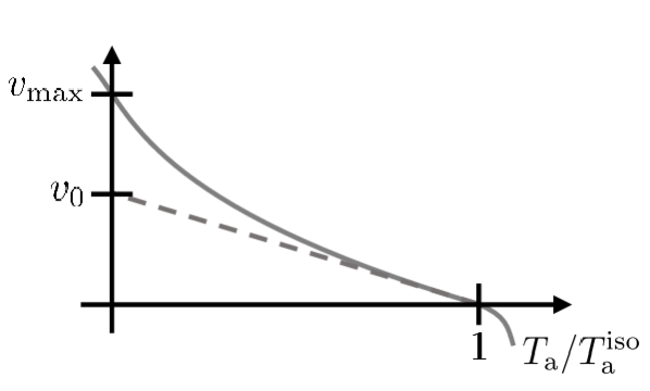
(a) Force-velocity relation

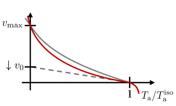
(b) reduced $v_{0}$

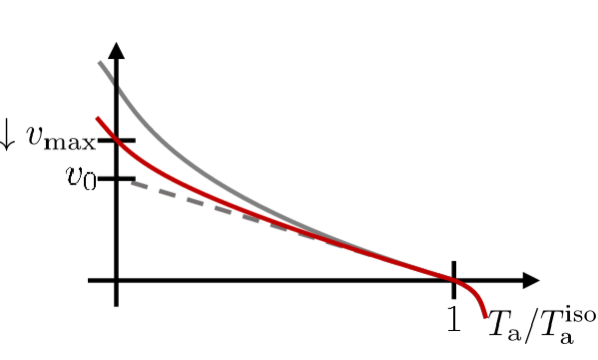
(c) reduced $v_{\mathrm{max}}$

Figure 8: Representation of the well-known force-velocity relationship of muscle cells. The normalized active tension $T_{\mathrm{a}}/T_{\mathrm{a}}^{\mathrm{iso}}$, where $T_{\mathrm{a}}^{\mathrm{iso}}$ denotes the force in isometric conditions, is a decreasing function of the shortening velocity $v$. As shown in the figure, $v_{\mathrm{max}}$ is the shortening velocity for which the active tension reaches zero, while $v_{0}$ is the slope of the curve in correspondence of the isometric conditions (i.e. $v=0$). (a) generic force-velocity relationship, (b) effect of reducing $v_{0}$ (in grey, the curve from (a)), (c) effect of reducing $v_{\mathrm{max}}$ (in grey, the curve from (a)).

Hence, starting from the B calibration, we modified the parameters to obtain a $v_{\mathrm{max}}$ and a $v_{0}$ equal to one-fourth of the original ones (see Table 3, column E). As evidenced in Table 4, with the setting E all biomarkers fall within physiological ranges (see also Figure 7). We believe that this result can be explained precisely by the mechanism of fibers-stretch-rate feedback, whereby regions of the tissue undergoing rapid shortening experience a decrease in developed force, thus promoting a more homogeneous shortening in space and without significant spikes in time, with a resulting viscous-like effect. In conclusion, blood flow is redistributed more evenly over the duration of the ejection phase.

Based on the very good match with the reference values of the different biomarkers, in this work we use the calibration E as the baseline for EM simulations.

4.3 Heart physiology and validation against clinical biomarkers

(a) $t=0.11$ s

(b) $t=0.25$ s

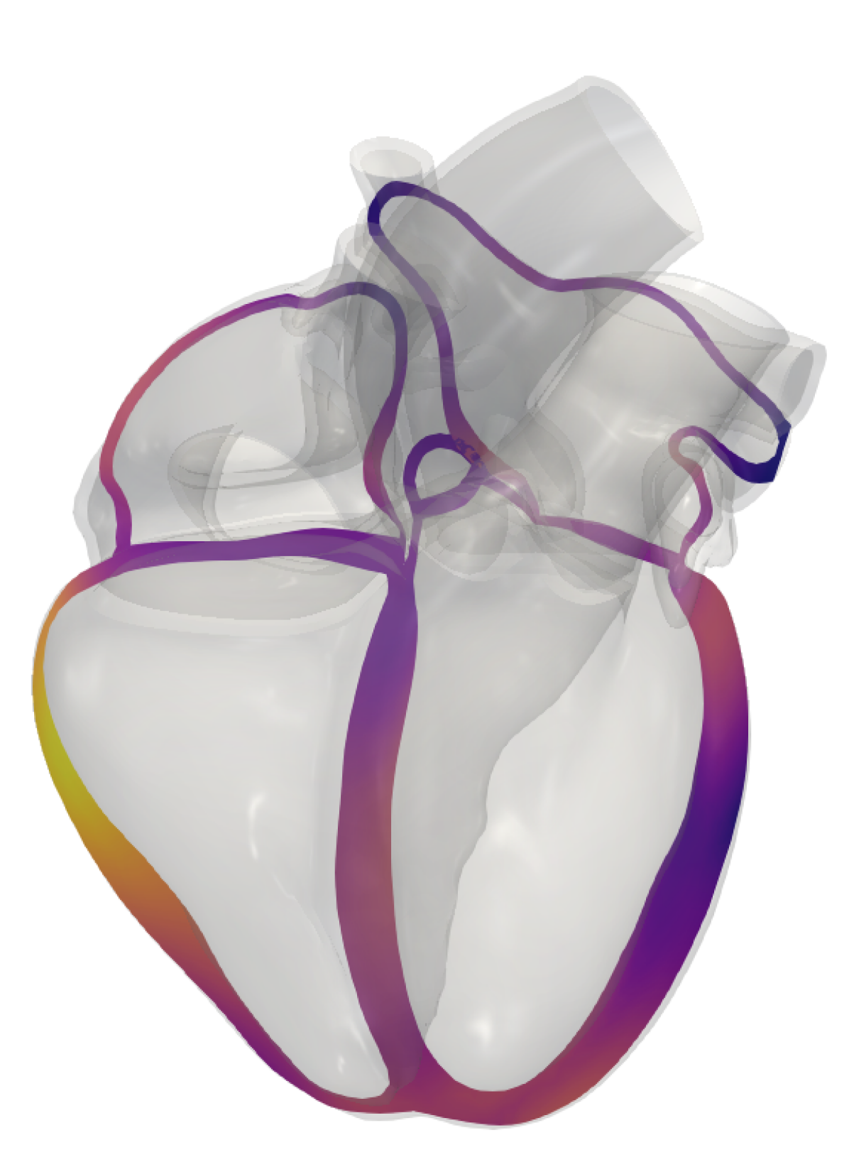
(c) $t=0.36$ s

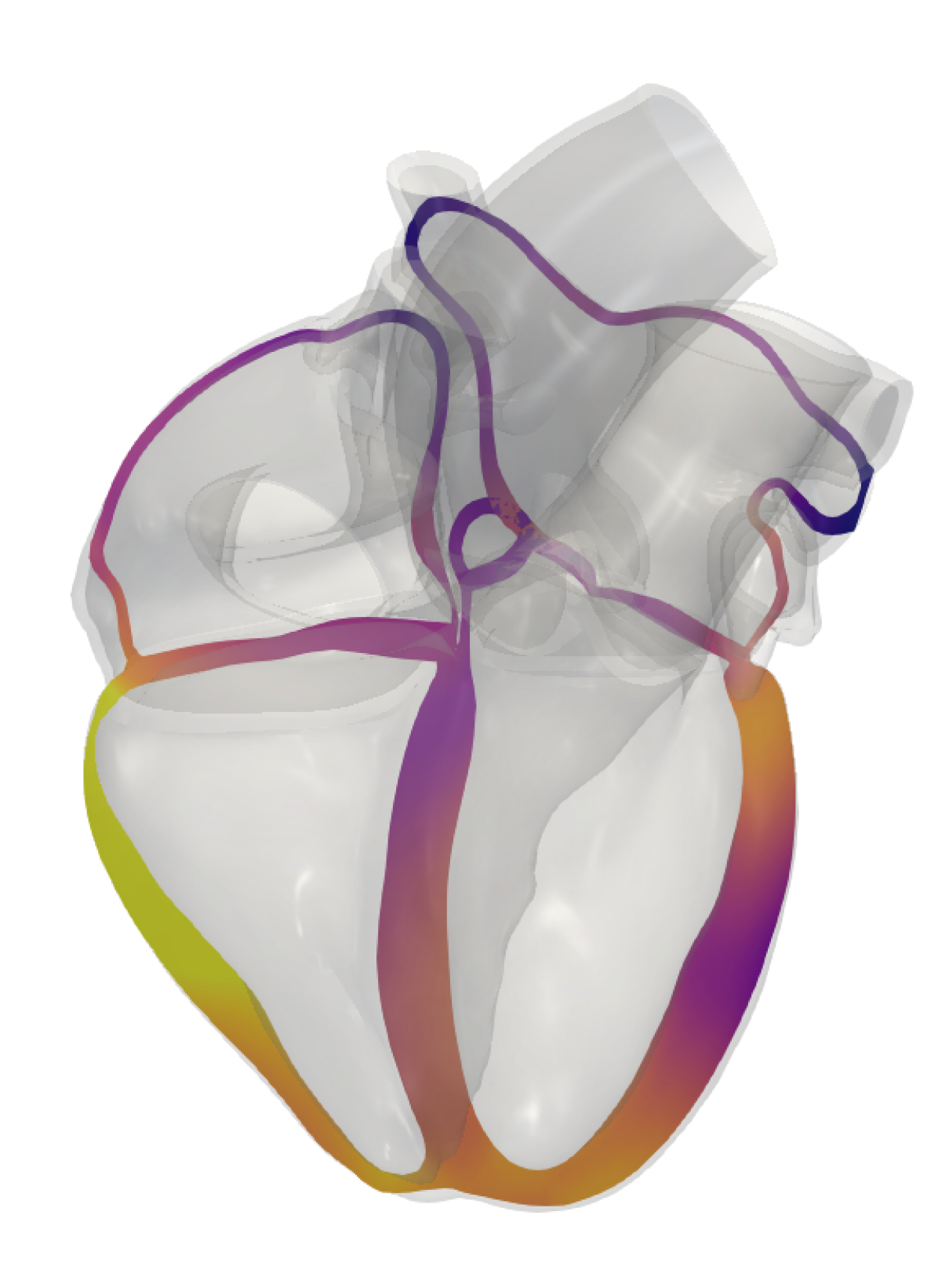
(d) $t=0.50$ s

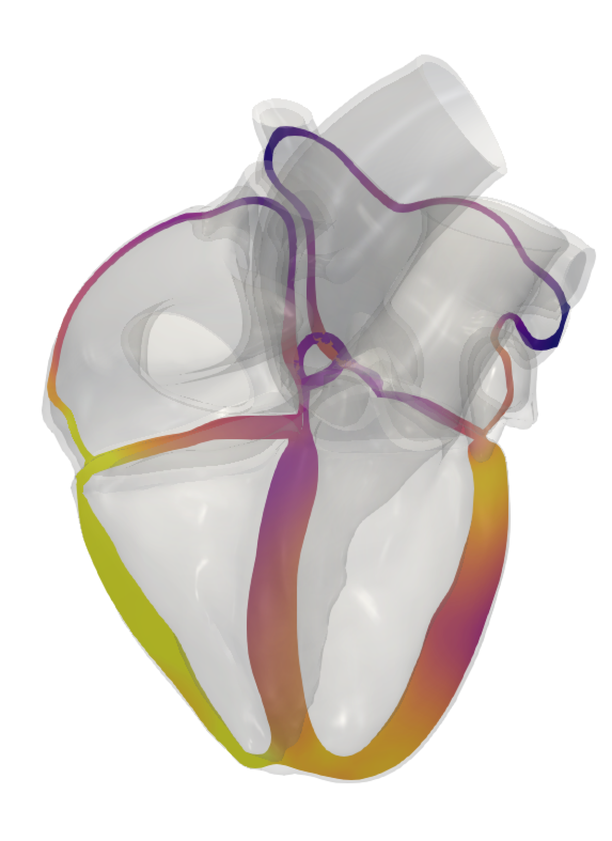
(e) $t=0.70$ s

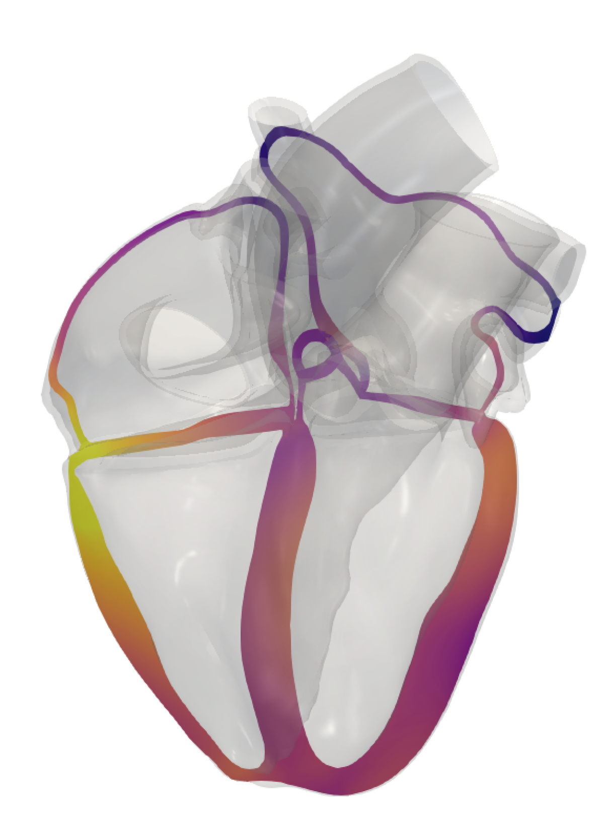
(f) $t=0.79$ s

Figure 9: Whole heart deformed with EM displacement (with respect to the reference stress-free configuration) and colored according to its magnitude for a single, representative heartbeat: (a) active atrial contraction, (b) isovolumetric contraction, (c) ejection (peak), (d) ejection (mid-deceleration), (e) isovolumetric relaxation, (f) passive ventricular filling.

$|\bm{d}^{\mathrm{EM}}|$ [mm]

Figure 9(f) shows the whole-heart EM displacement for a single, representative heartbeat, where we highlight six different phases: isovolumetric contraction, ejection (peak and mid-deceleration), isovolumetric relaxation, ventricular passive filling, and atrial contraction. As pointed out in [58], the whole-heart EM model can correctly reproduce the cardiac physiological motion. Moreover, as shown in Section 4.2, we found that, after a thorough calibration of the activation model, our numerical results are consistent with normal values found in literature in terms of several volumetric biomarkers.

In Figure 10, we report the volumes of the heart chambers and large arteries versus time, and we highlight time instants in which valves open and close. In Figure 13(f), we report the volume rendering of the velocity magnitude obtained with our EM-driven CFD simulation. We start our fluid dynamics simulation at the end of ventricular diastole.

During the active atrial contraction (Figure 13(a)), we observe the blood flowing from atria to ventricles, producing two high-speed jets in the MV and TV. This moment corresponds to the A-wave, as shown in Figure 12. In order to assess whether our numerical simulation is correctly reproducing the physiological heart function, we compare the peak velocities through valves with physiological ranges available in literature and acquired in healthy subjects. We report this comparison in Table 5. During diastole, we obtain lower velocities in the TV compared to MV, consistently with clinical measurements available in literature [123, 38].

During the isovolumetric contraction (Figure 13(b)), all valves are closed and the ventricular volumes remain constant. We measure lower velocity values compared to filling and ejection phases. Moreover, we found that the intraventricular pressure is not well defined and is prone to oscillations. As a matter of fact, since we are using EM as unidirectional input of the CFD model, the dynamic balance between hemodynamics and tissue mechanics is neglected. Furthermore, since we are modeling the cardiac valves with the RIIS method, weakly imposing a kinematic condition only, the dynamic balance is not fulfilled even between blood and valves. Thus, our computational model cannot correctly capture the physiological pressure transient during this phase, instead producing nonphysical and large oscillations. In Figure 11, we report the pressure transients in time and, for visualization purposes, we ignore the isovolumetric phases from the plot (grey boxes).

The ejection phase (Figure 13(c) and Figure 13(d)) is characterized by the opening of semilunar valves, the contraction of ventricles, and the blood flowing from the LV to the AO and from the RV to the PT. We measured peak flow rates equal to $398.74$ $\mathrm{mL}\text{/}\mathrm{s}$ and $478.16$ $\mathrm{mL}\text{/}\mathrm{s}$, in the AV and PV, respectively, consistently with physiological values [120]. Moreover, as shown in Table 5, we found that also maximum velocities between AV and PV and peak ventricular pressures during ejection are always in physiological ranges.

During the isovolumetric relaxation, both the atrioventricular and semilunar valves are closed. The velocities measured are low compared to those of the other phases of the heartbeat. Furthermore, as for the isovolumetric contraction, the computational model cannot reproduce the typical pressure decrease occurring in this phase. On the contrary, large pressure oscillations arise.

During the ventricular passive filling, the blood flows from the pulmonary veins and the venae cavae into the LA and RA, respectively. Moreover, the atrioventricular valves are open and high-speed jets form between their leaflets. This moment corresponds to the E-wave of diastole (see Figure 12). Consistently with clinical measurements, the computational model is able to correctly reproduce the formation of the clockwise jet in the LV, redirecting the blood towards the outflow tract [124, 125]. Furthermore, from Table 5, we can observe that maximum velocity between MV and TV leaflets are in the physiological ranges. Furthermore, we also report average atrial pressure values and we found a general good agreement with reference data, even if left atrial pressure is slightly larger than our reference.

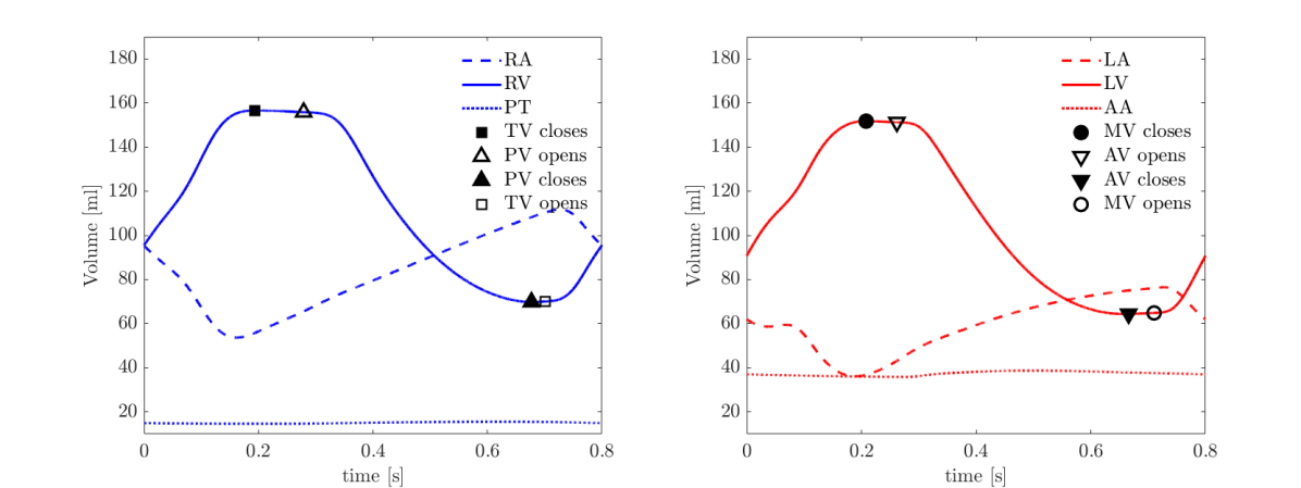
Figure 10: Volumes of RA, RV, PT (left) and LA, LV, AO (right) during a representative heartbeat. Valves open and close, instantaneously, at the initial and final times of isovolumetric phases. We report these times also in Table 2.

Biomarker		In silico	Physiological values
Peak MV velocity	[$\mathrm{m}\text{/}\mathrm{s}$]	1.03	0.89 $\pm$ 0.15	[123]
Peak AV velocity	[$\mathrm{m}\text{/}\mathrm{s}$]	1.21	1.07 $\pm$ 0.18	[126]
Peak TV velocity	[$\mathrm{m}\text{/}\mathrm{s}$]	0.45	0.48 $\pm$ 0.11	[127]
Peak PV velocity	[$\mathrm{m}\text{/}\mathrm{s}$]	1.15	0.80 to 1.20	[128]
Mean LA pressure	[$\mathrm{mmHg}\text{/}$]	13.3	2 to 12	[129]
Peak LV pressure	[$\mathrm{mmHg}\text{/}$]	111	119 $\pm$ 13	[121]
Mean RA pressure	[$\mathrm{mmHg}\text{/}$]	6.33	0 to 8	[129]
Peak RV pressure	[$\mathrm{mmHg}\text{/}$]	37.0	35 $\pm$ 11	[122]

Table 5: Fluid dynamics biomarkers obtained with the whole-heart CFD simulation (normal ranges or mean $\pm$ standard deviation). In silico values are computed by averaging fluid properties in spherical control volumes located between the valve leaflets (velocities) and in the heart chambers (pressures).

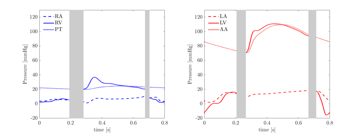
Figure 11: Pressure computed in control volumes located in RA, RV, PT (left) and LA, LV, AA (right) during a representative heartbeat. Isovolumetric phases are not considered, since the intraventricular pressure is not well defined when both valves are closed.

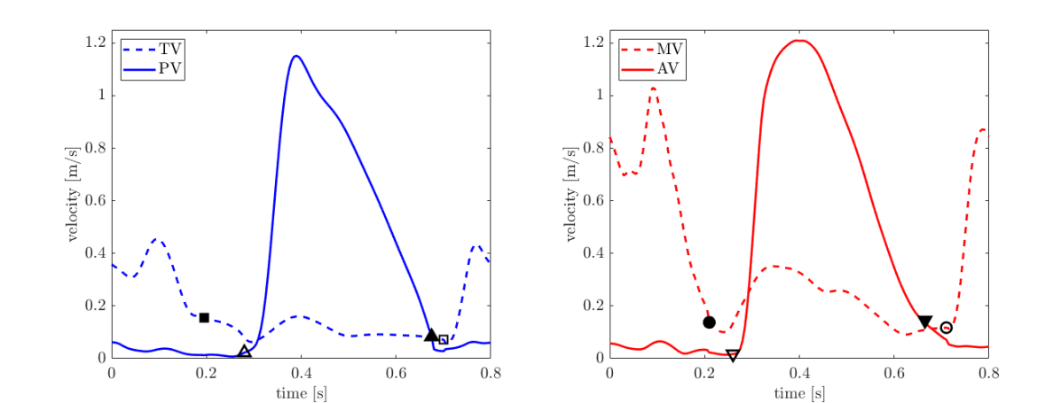
Figure 12: Velocity magnitudes computed in control volumes located between the valve leaflets: TV, PV (left) and MV, AV (right).

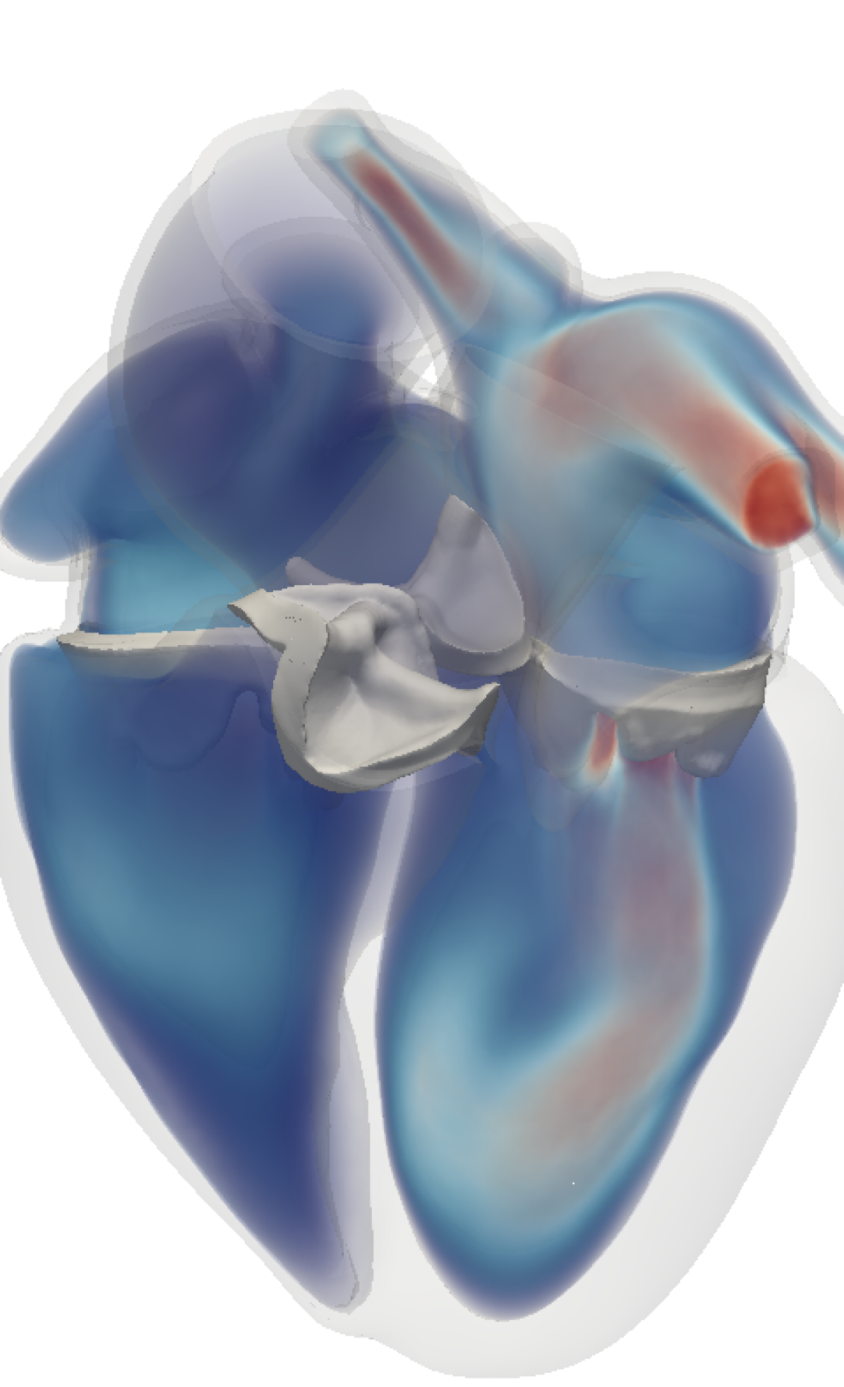
(a) $t=0.10$ s

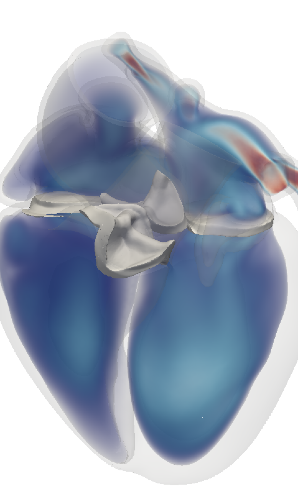
(b) $t=0.24$ s

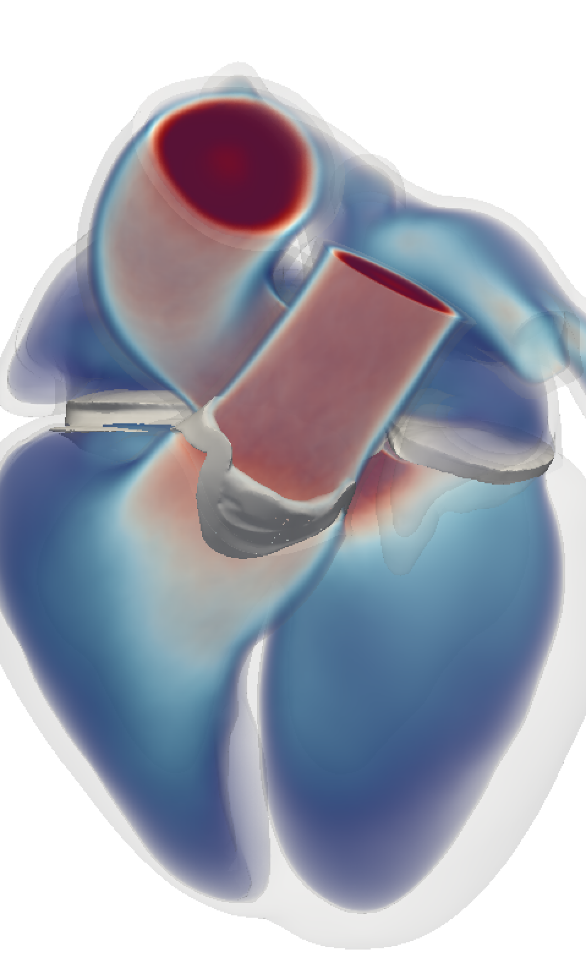
(c) $t=0.35$ s

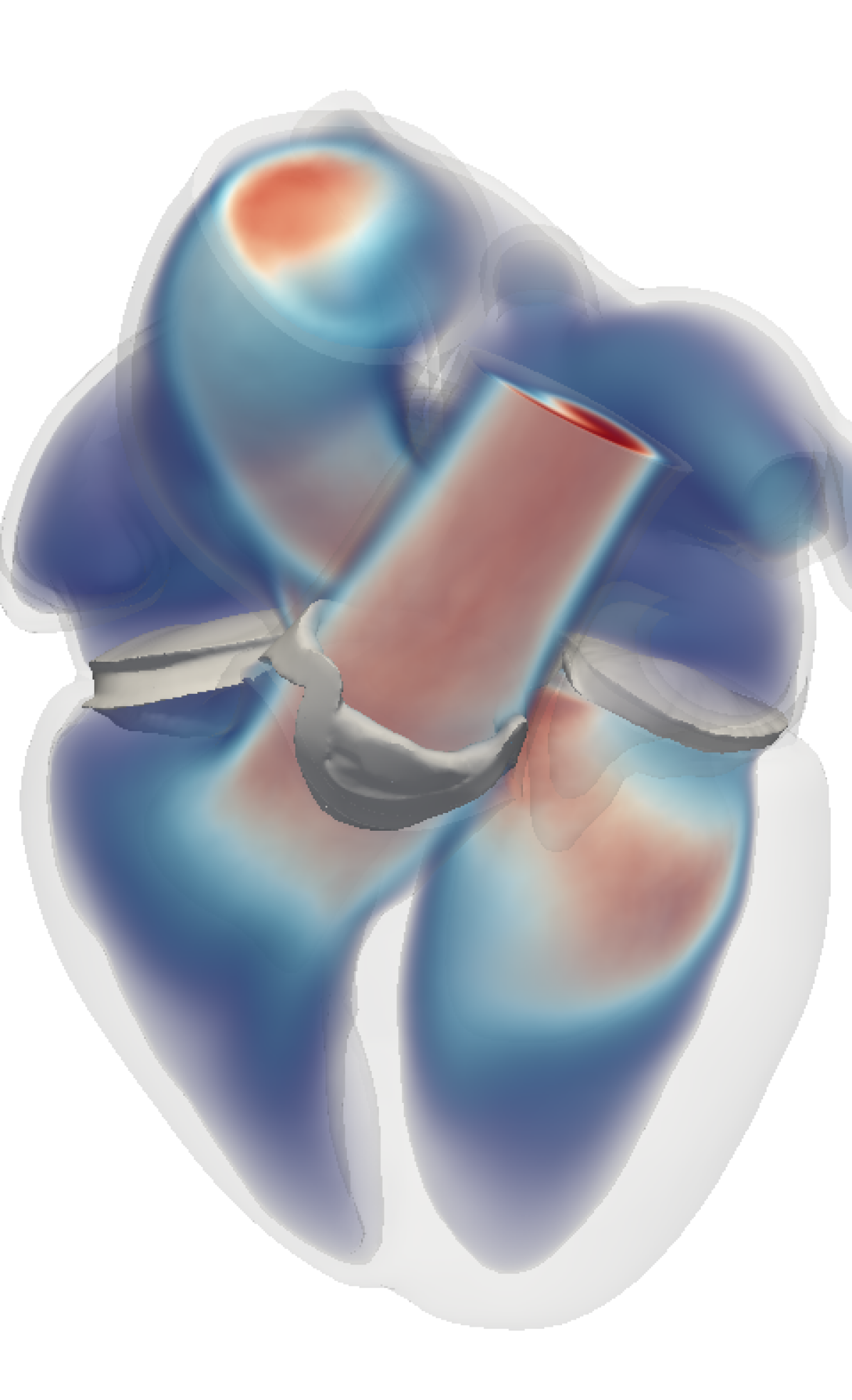
(d) $t=0.55$ s

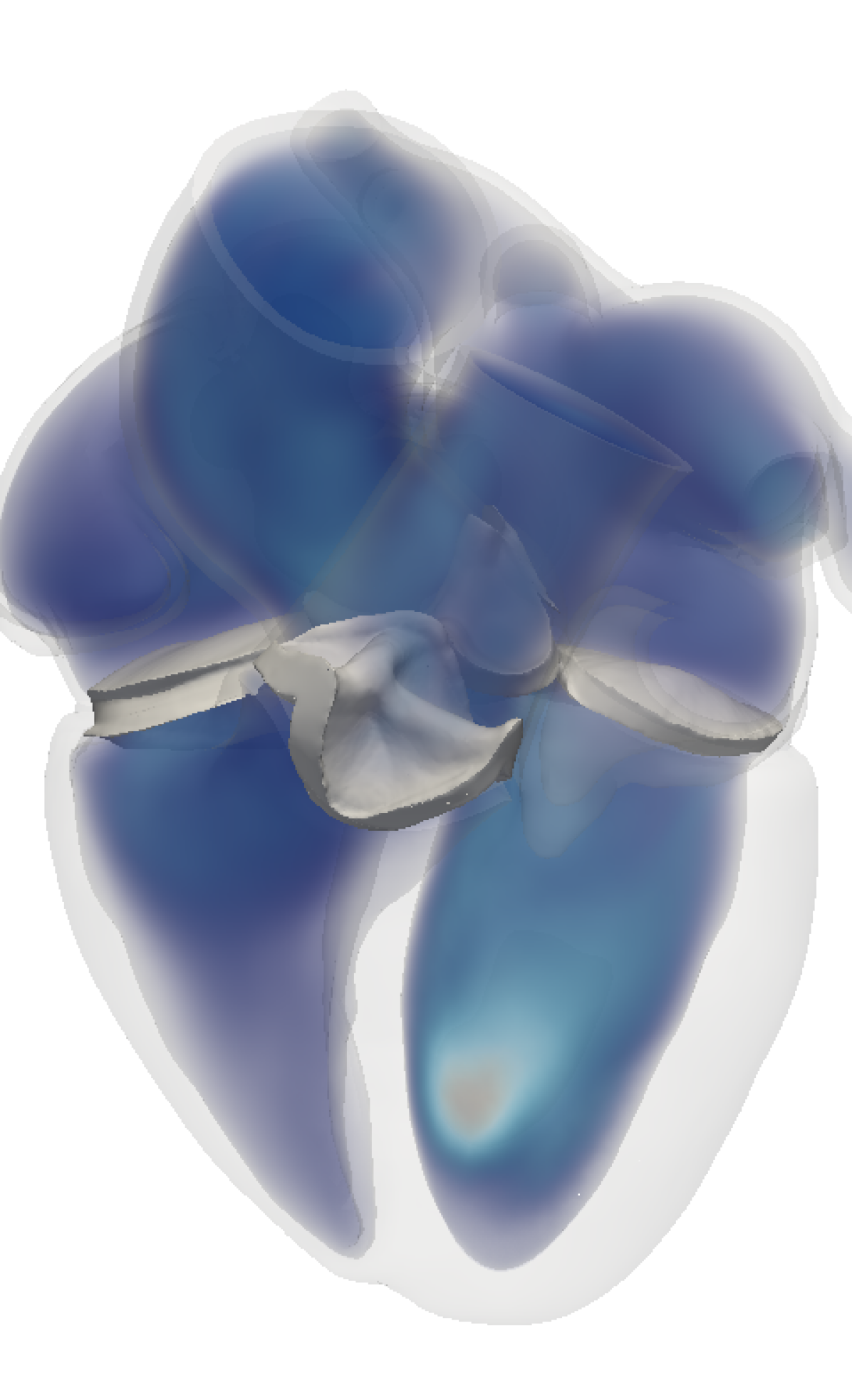
(e) $t=0.70$ s

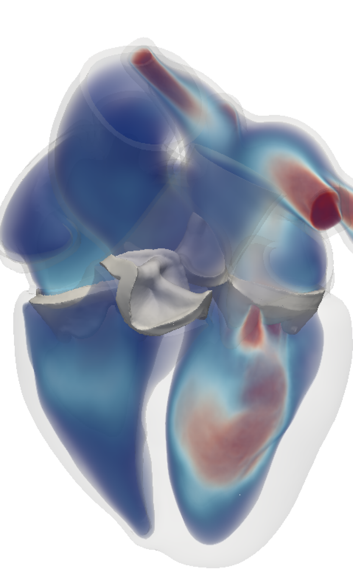
(f) $t=0.80$ s

Figure 13: Volume rendering of velocity magnitude in different frames during the cardiac cycle: (a) diastolic a-wave peak, (b) isovolumetric contraction, (c) systolic peak, (d) mid systolic deceleration, (e) isovolumetric relaxation, (f) diastolic a-wave peak.

$|\bm{u}|$ [m/s]

To better investigate blood flow patterns in the whole heart, we report the streamlines colored according to velocity magnitude in different chambers in Figure 14. We compare our in silico results with the MRI phase-velocity mapping visualization provided in Figure 1 of reference [125], and we found a good accordance. Specifically, Figure 14a shows the rotation of the blood in the RA as the chamber expands and the blood flows from the inferior and superior vena cava. Similarly, on the left side, the blood flows from the pulmonary veins to the expanding LA producing collision of blood jets and redirecting the flow towards the closed MV (see Figure 14b). During E-wave, as we show in Figure 14c, asymmetric recirculation is observed: shear layers roll through MV leaflets producing an O-vortex, as also seen in [1]. The counter-clockwise vortex under the posterior leaflet quickly disappears, and the clockwise vortex becomes larger and larger producing a clockwise jet, as described in [124], and clearly observed in Figure 14d.

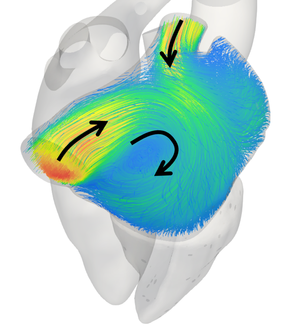
(a) Right atrium $t=0.6$ s

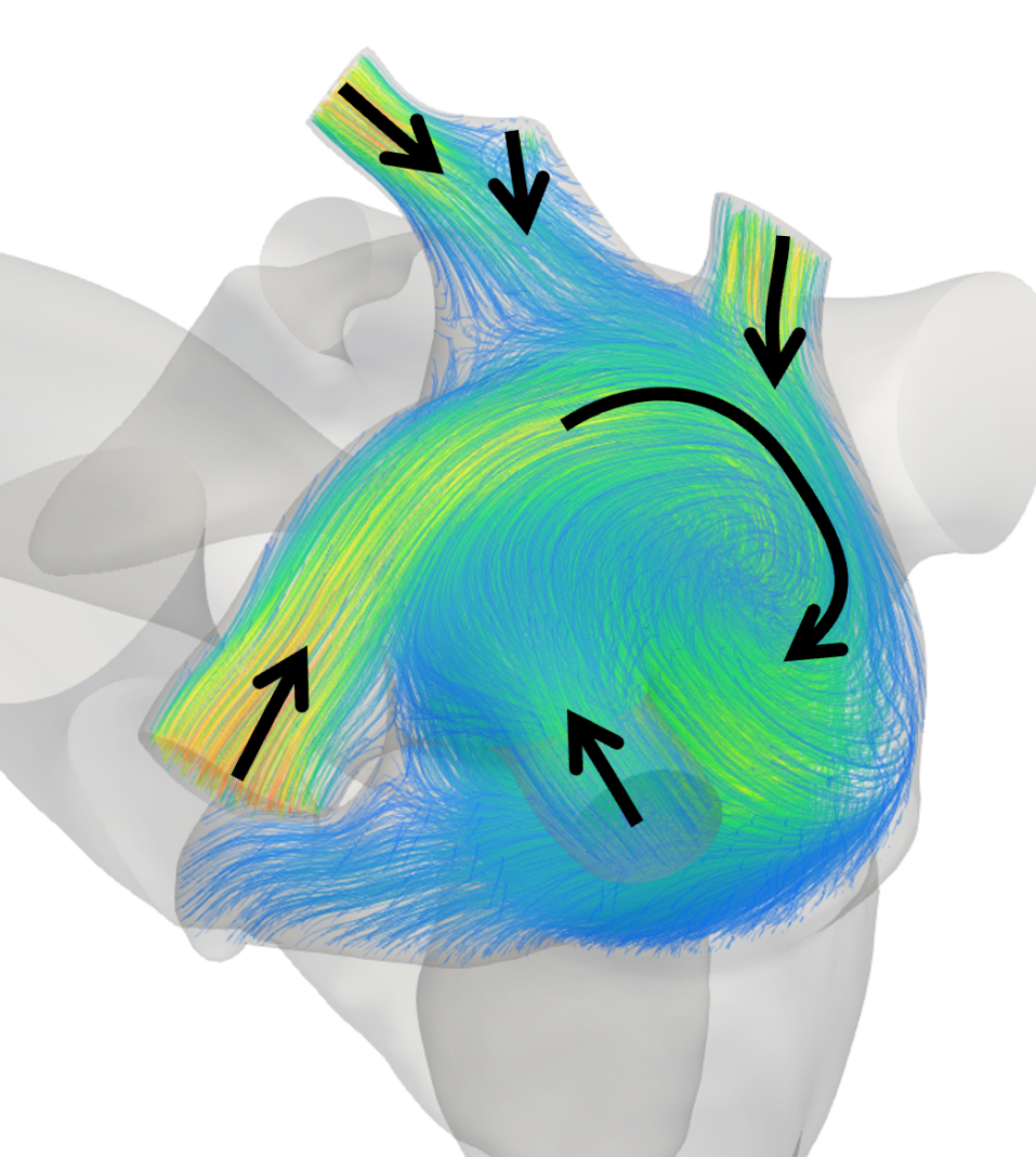
(b) Left atrium $t=0.6$ s

$|\bm{u}|$ [m/s]

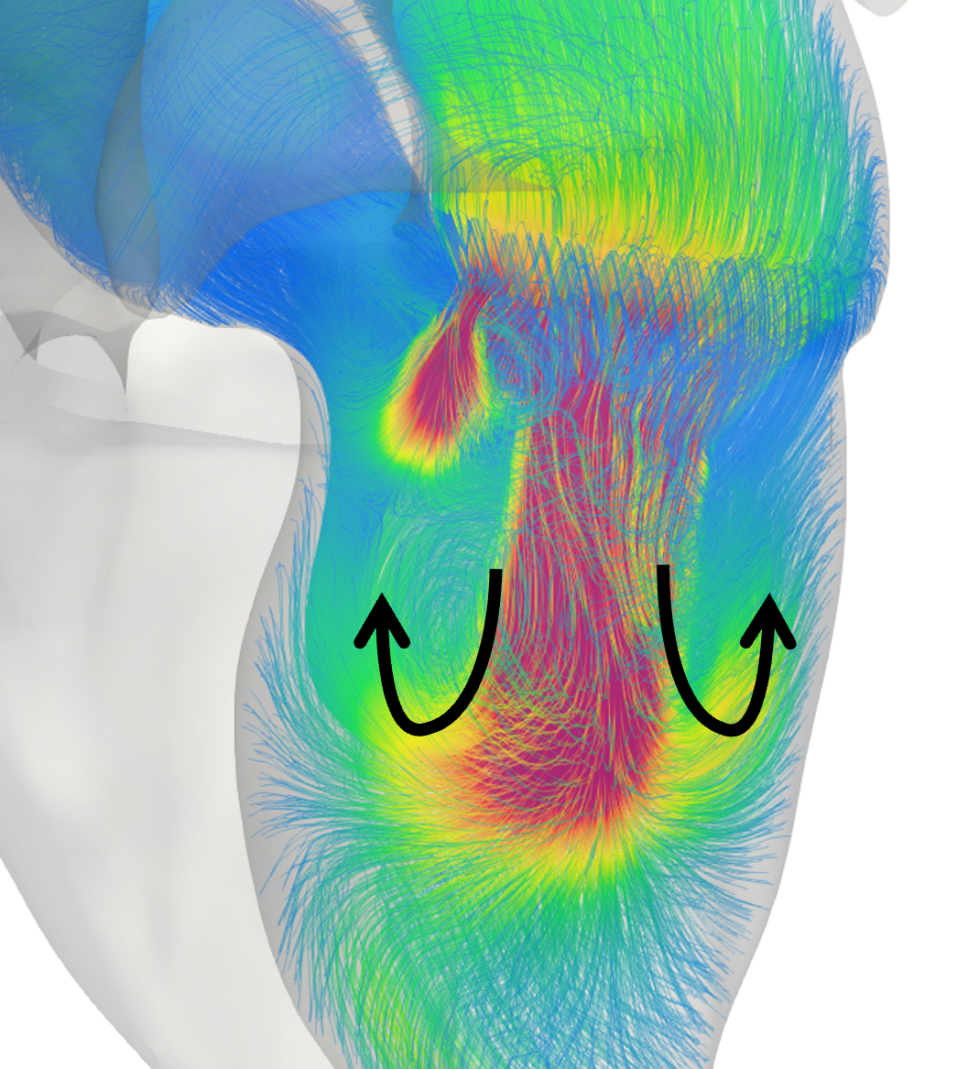
(c) Left ventricle $t=0.775$ s

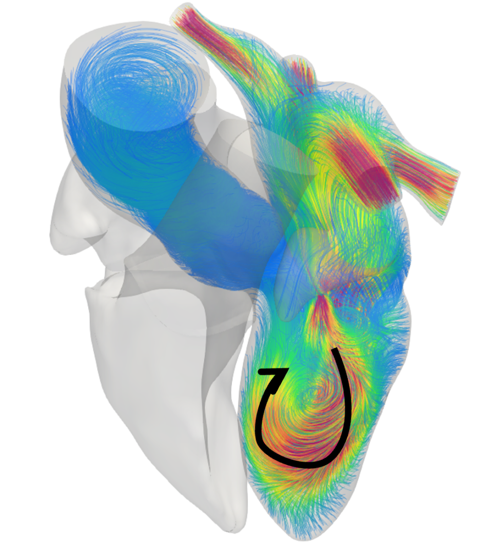
(d) Left heart $t=0.8$ s

$|\bm{u}|$ [m/s]

Figure 14: Streamlines colored according to velocity magnitude at different locations in the heart at different times: (a) right atrium during ventricular systole, (b) let atrium during ventricular systole, (c) clockwise and counter-clockwise vortices in the left ventricle during early diastole, (d) formation of clockwise jet in the left ventricle.

4.4 Application to a pathological scenario: Left Bundle Branch Block effects on hemodynamics

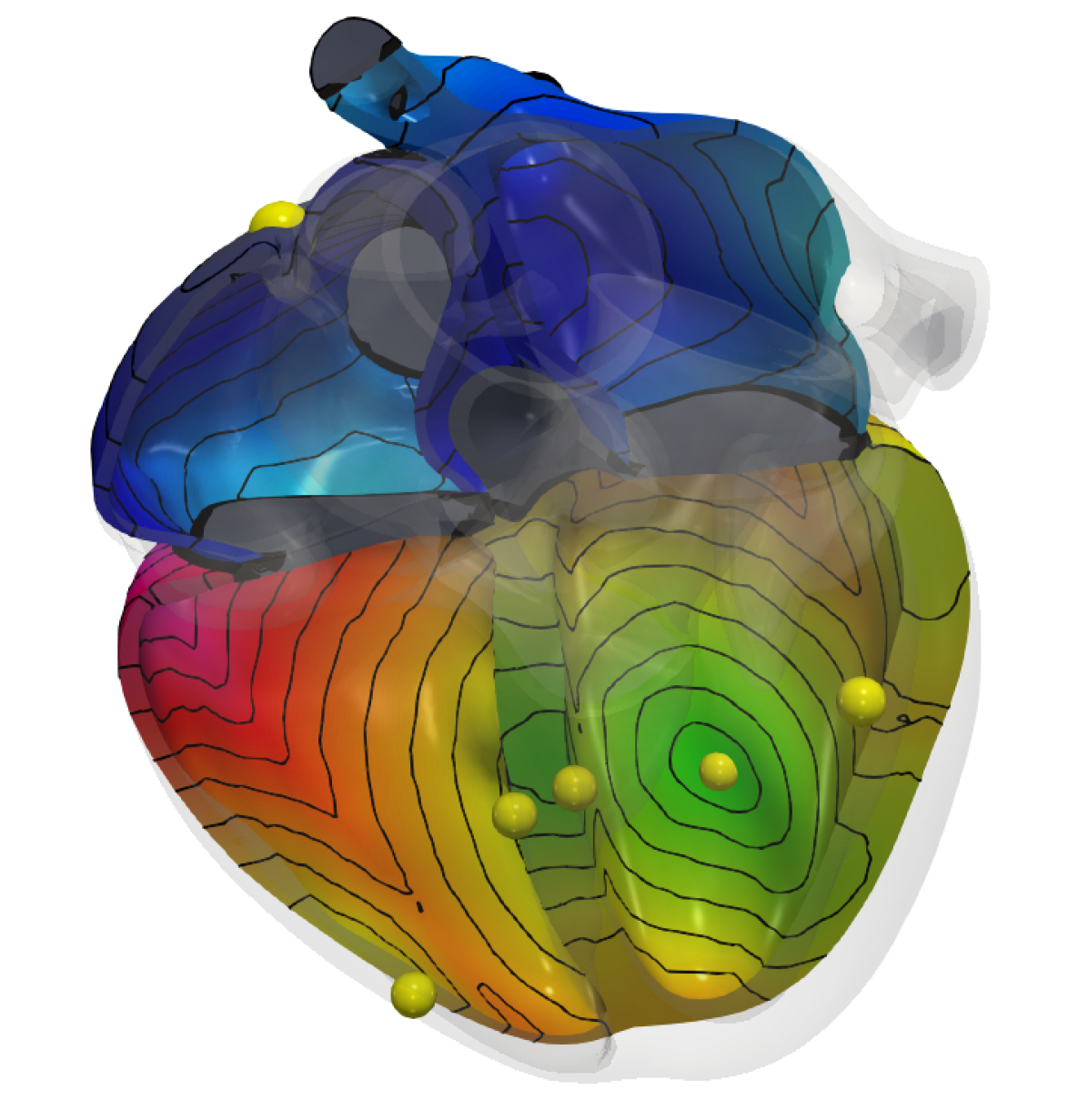
(a) physiological

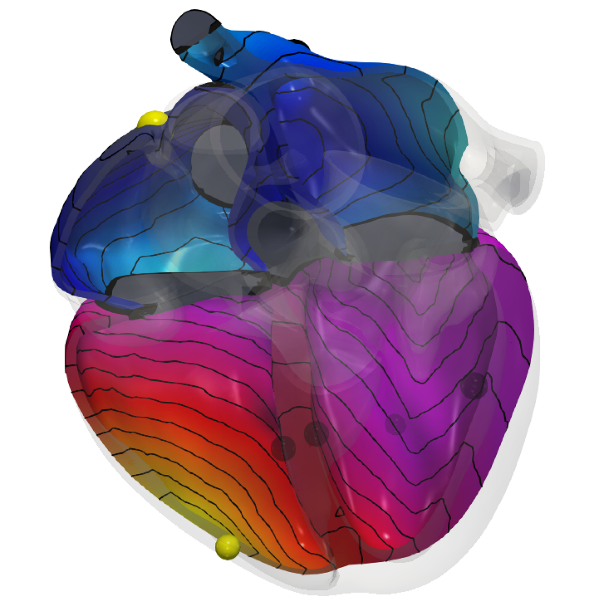
(b) LBBB

Figure 15: Activation maps and impulse sites (yellow spheres) in EM simulations; (a) physiological; (b) LBBB.

Activation time [ms]

In this section, we apply our multiphysics computational model to investigate the hemodynamic consequences of the LBBB. This heart condition is commonly associated to an electrophysiological abnormality; however, it implies a cascade of adverse events due to the interaction among different physical processes. LBBB consists in a slow or even absent conduction through the left bundle branch, causing a dyssynchronous contraction and relaxation of the left ventricle. Moreover, the LV dyssynchrony may have profound consequences on the heart hemodynamics, influencing flow patterns and, in turn, triggering heart remodeling [130, 131].

To simulate LBBB with our EM model, we deactivate the impulse sites in the LV and in the septum (see Figure 15(b)), so that the signal is generated by the SAN and the RVm sites solely. Our modeling choice is consistent with the work of [132], where a severe case of LBBB is accounted for by activating only one site in the RV free wall.

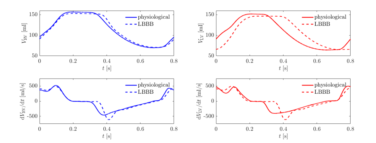
Figure 16: Ventricular volumes and ventricular volume derivatives for physiological and LBBB simulations.

Figure 16 displays volumes and their derivatives with respect to time for left and right ventricles, in both physiological and LBBB conditions. The electrical dyssynchrony between left and right parts produces a delay in the LV ejection and filling stages. Differently, no significant differences are observed in the RV volumes. Furthermore, compared to the physiological case (see Table 4) and consistently with [130], we measured reduced ejection fractions both in the right ($53.87$%) and left ($55.39$%) ventricles.

By means of our whole-heart EM driven CFD simulation, we can quantify how the pathology affects the endocardial wall stress. Let $\tau(\bm{u})=2\mu\epsilon(\bm{u})$ be the viscous stress tensor, we compute the wall shear stress vector as

$$\mathbf{WSS}(\bm{u})=\tau(\bm{u})\bm{n}-(\tau(\bm{u})\bm{n}\cdot\bm{n})\bm{n}\qquad\text{ on }\partial\Omega_{0}\times(0,T).$$

The time averaged wall shear stress (TAWSS) is then defined as

$$\mathrm{TAWSS}(\bm{u})=\frac{1}{T}\int_{0}^{T}|\mathbf{WSS}(\bm{u})|\,\mathrm{d}t\qquad\text{ on }\partial\Omega_{0}.$$

Figure 17(d) shows the TAWSS in the right and left heart in physiological conditions and under LBBB. We notice that the TAWSS distribution is almost unchanged for the right heart. Conversely, we find that LBBB alters the wall shear stress in correspondence of the LV septum, suggesting the potential occurrence of remodeling phenomena. In Figure 18, we report the minimum, maximum and average WSS in the LV septum against time, for the physiological and LBBB simulations. During the ejection, the WSS values are similar, while significant differences are present during the filling phase. As a matter of fact, under LBBB, the space-averaged WSS peak is 27.4% higher than the physiological case (see Figure 18, right). This is consistent with the work of Eriksson et al. (2017), where they observed, by means of 4Dflow MRI data, that LV dyssynchronous motion influences blood flow patterns during diastole, contributing to the development of cardiac remodeling [131].

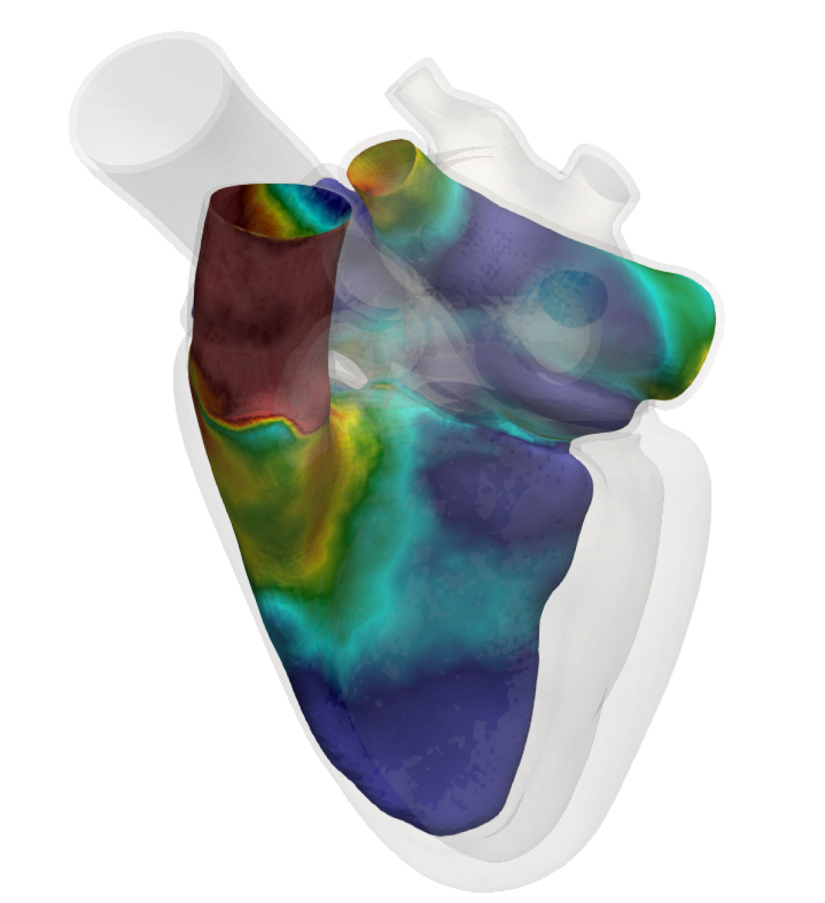
(a) physiological, RH

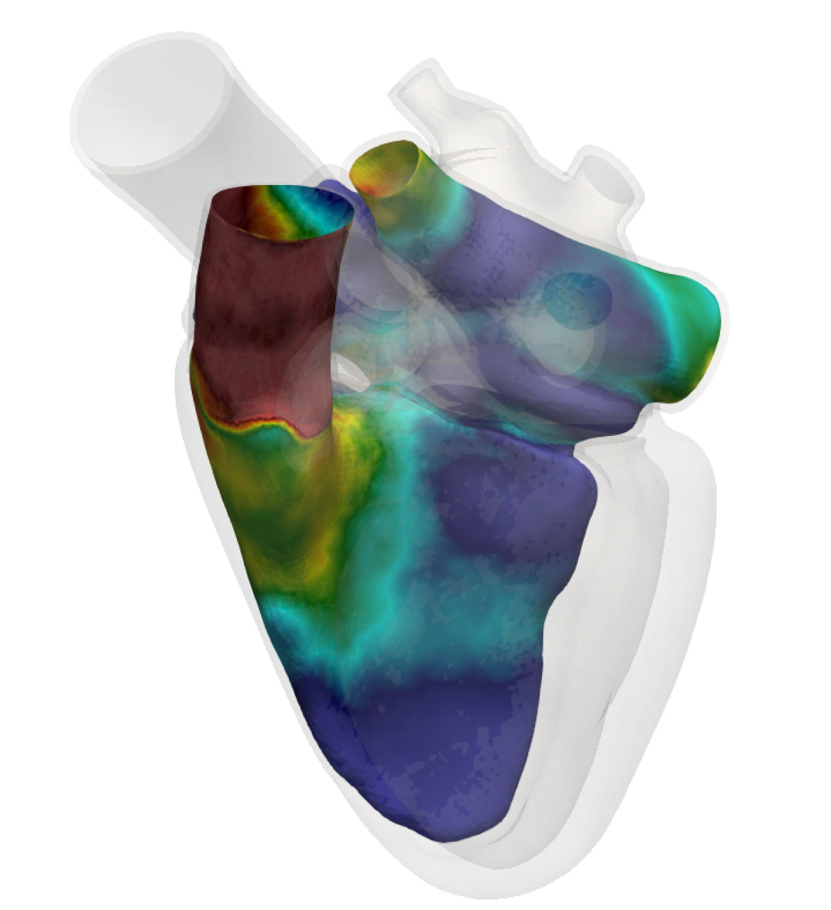
(b) LBBB, RH

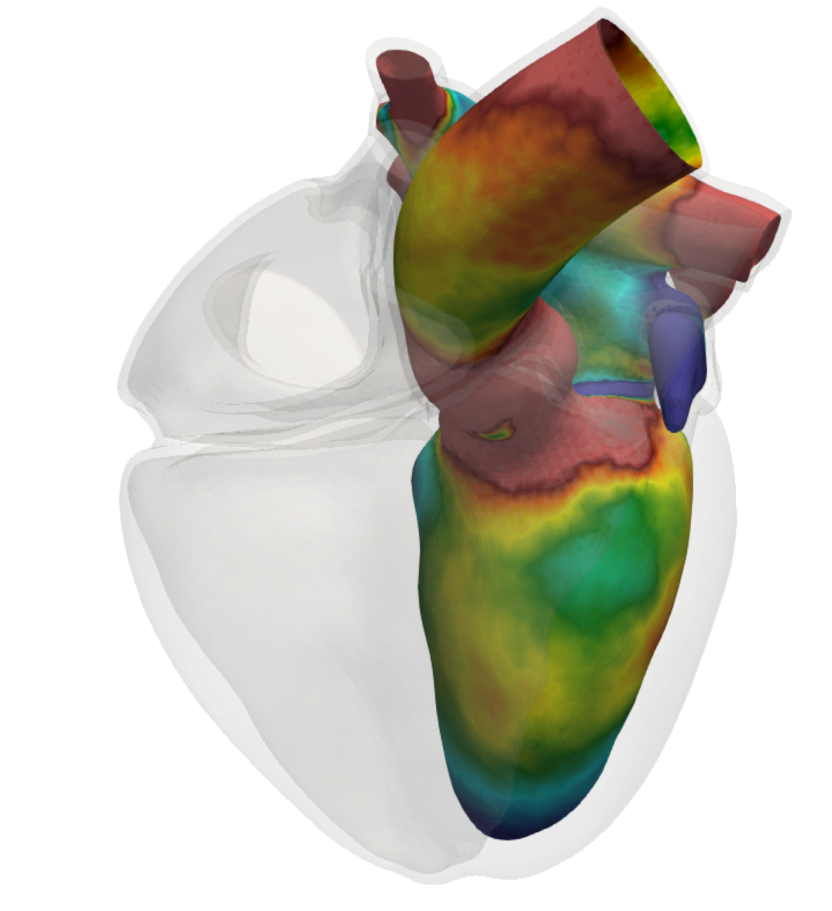
(c) physiological, LH

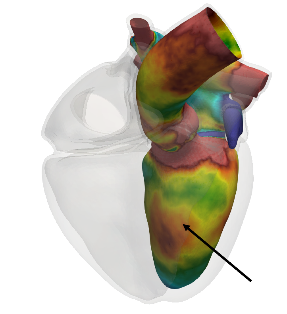
(d) LBBB, LH

Figure 17: TAWSS of the whole heart in physiological and pathological conditions for the LH and RH. Results obtained with whole-heart EM-driven CFD simulations, the left and right parts are separated for visualization purposes. The largest differences are observed in the LV septum, as highlighted by the black arrow.

$\mathrm{TAWSS}$ [Pa]

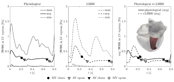
Figure 18: WSS in the LV septum over time. Maximum, average and minimum in physiological conditions (left); maximum, average and minimum in LBBB conditions (center); comparison between physiological and pathological conditions in terms of average values (right). The WSS is computed in the red portion shown on the right. In terms of maximum values, the pathological peak is 12.7% larger than the physiological case (cf. left and center figures). The average WSS peak increases of 27.4% (right figure).

5 Limitations and further developments

We discuss some limitations of our study. The computational model introduced cannot fully represent the isovolumetric phases in terms of pressure. Indeed, when both valves are closed and the ventricles are contracting/relaxing at constant volumes, the pressure is not well-defined, and thus prone to spurious oscillations. This is due to the fact that we are using kinematic conditions only in all the ventricular boundaries. Indeed, we prescribe the EM displacement on the endocardium and endothelium, and we model valves with the RIIS method using a penalty-based kinematic condition. The oscillatory pressure during such phases does not influence the velocity field. However, it prevents from using the simulated pressure values to choose when to open and close the valves, forcing hence to prescribe a-priori opening and closing times. The use of bidirectionally coupled FSI models for the blood-myocardium or blood-valve systems (or for both of them) may allow to correctly capture the pressure transient during these phases, as seen for instance in [42] where a fully-coupled electro-mechano-fluid of the heart is considered.

Moreover, we noticed that the ejection phase is too slow and the ventricular passive filling too fast, if compared with medical literature values. Consequently, E-wave and A-wave are characterized by comparable amplitudes, whereas the EA ratio should be approximately equal to 1.30 $\pm$ 0.570 [123]. In this respect, we believe that the use of ionic models with a more realistic decrease of calcium concentration is essential to better capture these phenomena.

Finally, we applied the computational model to a realistic, templated heart geometry. In order to move towards the realization of whole-heart digital twins, further developments should involve patient-specific cardiac simulations, accompanied with a stringent process of data assimilation, model validation and uncertainty quantification.

6 Conclusions

In this paper, we introduced a computational model for the hemodynamics simulation of the whole human heart accounting for the main features affecting the intracardiac flows. We considered a realistic whole-heart geometry, and we employed a four-chamber 3D-0D electromechanical model to provide the displacement as input to the cardiac CFD model. We modelled the effect of cardiac valves in the fluid via a resistive immersed method and we accounted for transition-to-turbulence regime through the VMS-LES method. Moreover, for the first time, we coupled the 3D CFD model of the whole heart to the surrounding closed-loop circulation, to get a geometric multiscale 3D-0D hemodynamic model of the entire cardiovascular system. We solved our multiphysics and multiscale computational model using our in-house finite element library life${}^{\texttt{x}}$.

We introduced a calibration of the activation model, driving the electromechanical simulation, aimed at obtaining physiological realistic flowrates, and consequently blood velocities, in the CFD simulation. Our calibration highlights the effect of the parameters of the active force generation model, associated to the microscopic features of its kinematics and of the force-velocity relationship, on the macroscopic heartbeat indicators.

We carried out EM-driven CFD simulation on a realistic whole-heart geometry and we showed that the computational model can correctly reproduce blood velocities and pressure traces when we compare the results with clinical ranges from medical literature. Furthermore, we found that the computational model captures typical blood flow patterns observed in MRI phase-velocity mapping visualizations.

Finally, we applied the whole-heart model to simulate the pathological scenario of Left Bundle Branch Block: we correctly predicted the electrical delay, the consequent mechanical dyssynchrony, a reduced ejection fraction, and an increasing wall shear stress in the left ventricular septum during the filling stage. Overall, this study confirms that the interaction of different physics in a high-fidelity integrated whole-heart model is essential for simulating the cardiac function, allowing to faithfully capture pathological events occurring at different physical levels.

Appendix A The open 0D circulation model

The closed-loop lumped-parameter (0D) circulation model that we employ was proposed in [59] and inspired by [51, 133]. To couple the 0D model to the 3D model of the heart, we follow the same steps presented in [26]. Specifically, the open 0D system we get reads as follows: for any $t\in(0,T)$,

$$\frac{\mathrm{d}p_{\text{AR}}^{\text{SYS}}(t)}{\mathrm{d}t} =\frac{1}{C_{\text{AR}}^{\text{SYS}}}\left(Q_{\text{AV}}(t)-Q_{\text{AR}}^{\text{SYS}}(t)\right),$$ (7a)

$$\frac{\mathrm{d}p_{\text{VEN}}^{\text{SYS}}(t)}{\mathrm{d}t} =\frac{1}{C_{\text{VEN}}^{\text{SYS}}}\left(Q_{\text{AR}}^{\text{SYS}}(t)-Q_{\text{VEN}}^{\text{SYS}}(t)\right),$$ (7b)

$$\frac{\mathrm{d}p_{\text{AR}}^{\text{PUL}}(t)}{\mathrm{d}t} =\frac{1}{C_{\text{AR}}^{\text{PUL}}}\left(Q_{\text{PV}}(t)-Q_{\text{AR}}^{\text{PUL}}(t)\right),$$ (7c)

$$\frac{\mathrm{d}p_{\text{VEN}}^{\text{PUL}}(t)}{\mathrm{d}t} =\frac{1}{C_{\text{VEN}}^{\text{PUL}}}\left(Q_{\text{AR}}^{\text{PUL}}(t)-Q_{\text{PUL}}^{\text{VEN, 3D}}(t)\right),$$ (7d)

$$\frac{\mathrm{d}Q_{\text{AR}}^{\text{SYS}}(t)}{\mathrm{d}t} =\frac{R_{\text{AR}}^{\text{SYS}}}{L_{\text{AR}}^{\text{SYS}}}\left(-Q_{\text{AR}}^{\text{SYS}}(t)-\frac{p_{\text{VEN}}^{\text{SYS}}(t)-p_{\text{AR}}^{\text{SYS}}(t)}{R_{\text{AR}}^{\text{SYS}}}\right),$$ (7e)

$$\frac{\mathrm{d}Q_{\text{AR}}^{\text{PUL}}(t)}{\mathrm{d}t} =\frac{R_{\text{AR}}^{\text{PUL}}}{L_{\text{AR}}^{\text{PUL}}}\left(-Q_{\text{AR}}^{\text{PUL}}(t)-\frac{p_{\text{VEN}}^{\text{PUL}}(t)-p_{\text{AR}}^{\text{PUL}}(t)}{R_{\text{AR}}^{\text{PUL}}}\right),$$ (7f)

solved with suitable initial conditions, and

$$p_{\text{LA}}^{\text{in}}(t) =p_{\text{VEN}}^{\text{PUL}}(t)-R_{\text{VEN}}^{\text{PUL}}Q_{\text{VEN}}^{\text{PUL}}(t)-L_{\text{VEN}}^{\text{PUL}}\dfrac{\mathrm{d}Q_{\text{VEN}}^{\text{PUL, 3D}}(t)}{\mathrm{d}t},$$ (8a)

$$p_{\text{RA}}^{\text{in}}(t) =p_{\text{VEN}}^{\text{SYS}}(t)-R_{\text{VEN}}^{\text{SYS}}Q_{\text{VEN}}^{\text{SYS}}(t)-L_{\text{VEN}}^{\text{SYS}}\dfrac{\mathrm{d}Q_{\text{VEN}}^{\text{SYS, 3D}}(t)}{\mathrm{d}t}.$$ (8b)

Appendix B Setup of EM and CFD simulations

We report in this section the values of the parameters used in the EM and CFD simulations.

Table 6 reports the parameters for the circulation model used in the EM simulation. With respect to the model presented in [58], we introduce two additional resistance elements ($R_{\text{upstream}}^{\text{SYS}}$ and $R_{\text{upstream}}^{\text{PUL}}$) and two inductance elements ($L^{\text{AV}}$, $L^{\text{PV}}$, see Figure 1c). They have the purpose of making the 0D circulation model, which surrogates the fluid dynamics, as similar as possible to the 3D CFD problem. For the same reason, the minimum resistances of the non-ideal diodes representing the AV and PV are increased with respect to [58].

The calibration of the RDQ20 activation model is extensively discussed in Section 4.2, and the corresponding parameter values are reported in Table 3. As reference sarcomere length, we set $\mathrm{SL}_{0}$ = $2.2$ $\mathrm{\SIUnitSymbolMicro m}\text{/}$. For all other parameters in the EM model, we use the same values as those of the baseline simulation of [58].

Table 7 reports the values of the initial circulation states for the CFD simulation. They are taken equal to the values reached at the beginning of the last heartbeat in the EM simulation. All resistance, capacitance and inductance parameters are the same as in the EM model (see Table 6).

	Parameter	Value
Systemic arteries	$R_{\text{AR}}^{\text{SYS}}$	0.48	$\mathrm{mmHg}\text{\,}\mathrm{s}\text{/}\mathrm{ml}$
	$C_{\text{AR}}^{\text{SYS}}$	1.50	$\mathrm{ml}\text{/}\mathrm{mmHg}$
	$L_{\text{AR}}^{\text{SYS}}$	0.005	$\mathrm{mmHg}\text{\,}{\mathrm{s}}^{2}\text{/}\mathrm{ml}$
	$R_{\text{upstream}}^{\text{SYS}}$	0.048	$\mathrm{mmHg}\text{\,}\mathrm{s}\text{/}\mathrm{ml}$
	$p_{\text{AR, 0}}^{\text{SYS}}$	83.9	$\mathrm{mmHg}\text{/}$
	$Q_{\text{AR, 0}}^{\text{SYS}}$	0.0	$\mathrm{ml}\text{/}\mathrm{s}$
Systemic veins	$R_{\text{VEN}}^{\text{SYS}}$	0.26	$\mathrm{mmHg}\text{\,}\mathrm{s}\text{/}\mathrm{ml}$
	$C_{\text{VEN}}^{\text{SYS}}$	60	$\mathrm{ml}\text{/}\mathrm{mmHg}$
	$L_{\text{VEN}}^{\text{SYS}}$	$5\text{⋅}{10}^{-4}$	$\mathrm{mmHg}\text{\,}{\mathrm{s}}^{2}\text{/}\mathrm{ml}$
	$p_{\text{VEN, 0}}^{\text{SYS}}$	35.5	$\mathrm{mmHg}\text{/}$
	$Q_{\text{VEN, 0}}^{\text{SYS}}$	0.0	$\mathrm{ml}\text{/}\mathrm{s}$
Pulmonary arteries	$R_{\text{AR}}^{\text{PUL}}$	0.032116	$\mathrm{mmHg}\text{\,}\mathrm{s}\text{/}\mathrm{ml}$
	$C_{\text{AR}}^{\text{PUL}}$	10	$\mathrm{ml}\text{/}\mathrm{mmHg}$
	$L_{\text{AR}}^{\text{PUL}}$	0.0005	$\mathrm{mmHg}\text{\,}{\mathrm{s}}^{2}\text{/}\mathrm{ml}$
	$R_{\text{upstream}}^{\text{PUL}}$	0.0032116	$\mathrm{mmHg}\text{\,}\mathrm{s}\text{/}\mathrm{ml}$
	$p_{\text{AR, 0}}^{\text{PUL}}$	14.90	$\mathrm{mmHg}\text{/}$
	$Q_{\text{AR, 0}}^{\text{PUL}}$	0.0	$\mathrm{ml}\text{/}\mathrm{s}$
Pulmonary veins	$R_{\text{VEN}}^{\text{PUL}}$	0.035684	$\mathrm{mmHg}\text{\,}\mathrm{s}\text{/}\mathrm{ml}$
	$C_{\text{VEN}}^{\text{PUL}}$	16	$\mathrm{ml}\text{/}\mathrm{mmHg}$
	$L_{\text{VEN}}^{\text{PUL}}$	0.0005	$\mathrm{mmHg}\text{\,}{\mathrm{s}}^{2}\text{/}\mathrm{ml}$
	$p_{\text{VEN, 0}}^{\text{PUL}}$	13.58	$\mathrm{mmHg}\text{/}$
	$Q_{\text{VEN, 0}}^{\text{PUL}}$	0.0	$\mathrm{ml}\text{/}\mathrm{s}$
Valves	$R_{\min}^{\mathrm{MV}}$	0.0075	$\mathrm{mmHg}\text{\,}\mathrm{s}\text{/}\mathrm{ml}$
	$R_{\min}^{\mathrm{AV}}$	0.0355	$\mathrm{mmHg}\text{\,}\mathrm{s}\text{/}\mathrm{ml}$
	$R_{\min}^{\mathrm{TV}}$	0.0075	$\mathrm{mmHg}\text{\,}\mathrm{s}\text{/}\mathrm{ml}$
	$R_{\min}^{\mathrm{PV}}$	0.0184	$\mathrm{mmHg}\text{\,}\mathrm{s}\text{/}\mathrm{ml}$
	$R_{\max}^{\mathrm{MV}}$, $R_{\max}^{\mathrm{AV}}$, $R_{\max}^{\mathrm{TV}}$, $R_{\max}^{\mathrm{PV}}$	75006.2	$\mathrm{mmHg}\text{\,}\mathrm{s}\text{/}\mathrm{ml}$
	$L^{\mathrm{AV}}$, $L^{\mathrm{PV}}$	$5\text{⋅}{10}^{-4}$	$\mathrm{mmHg}\text{\,}{\mathrm{s}}^{2}\text{/}\mathrm{ml}$

Table 6: Parameters and initial conditions of the circulation model used for the EM simulation.

	Parameter	Value
Systemic arteries	$p_{\text{AR, 0}}^{\text{SYS}}$	86.3480	$\mathrm{mmHg}\text{/}$
	$Q_{\text{AR, 0}}^{\text{SYS}}$	109.6429	$\mathrm{ml}\text{/}\mathrm{s}$
Systemic veins	$p_{\text{VEN, 0}}^{\text{SYS}}$	34.4923	$\mathrm{mmHg}\text{/}$
	$Q_{\text{VEN, 0}}^{\text{SYS}}$	112.9209	$\mathrm{ml}\text{/}\mathrm{s}$
Pulmonary arteries	$p_{\text{AR, 0}}^{\text{PUL}}$	22.2310	$\mathrm{mmHg}\text{/}$
	$Q_{\text{AR, 0}}^{\text{PUL}}$	83.2132	$\mathrm{ml}\text{/}\mathrm{s}$
Pulmonary veins	$p_{\text{VEN, 0}}^{\text{PUL}}$	19.5813	$\mathrm{mmHg}\text{/}$
	$Q_{\text{VEN, 0}}^{\text{PUL}}$	262.6397	$\mathrm{ml}\text{/}\mathrm{s}$

Table 7: Initial states of the circulation model for the CFD simulation. The values are equal to those of the circulation state variables at the beginning of the last heartbeat in the EM simulation. All remaining circulation parameters (resistances, capacitances, inductances) are the same as in the EM model (see Table 6).

References

- [1] Christophe Chnafa, Simon Mendez and Franck Nicoud “Image-based large-eddy simulation in a realistic left heart” In Computers & Fluids 94 Elsevier, 2014, pp. 173–187
- [2] Alexandre This, Ludovic Boilevin-Kayl, Miguel A Fernández and Jean-Frédéric Gerbeau “Augmented Resistive Immersed Surfaces valve model for the simulation of cardiac hemodynamics with isovolumetric phases” In International Journal for Numerical Methods in Biomedical Engineering 36.3 Wiley Online Library, 2020, pp. e3223
- [3] Anna Tagliabue, Luca Dede’ and Alfio Quarteroni “Complex blood flow patterns in an idealized left ventricle: A numerical study” In Chaos: An Interdisciplinary Journal of Nonlinear Science 27.9 AIP Publishing LLC, 2017, pp. 093939
- [4] Anna Tagliabue, Luca Dede’ and Alfio Quarteroni “Fluid dynamics of an idealized left ventricle: the extended Nitsche’s method for the treatment of heart valves as mixed time varying boundary conditions” In International Journal for Numerical Methods in Fluids 85.3 Wiley Online Library, 2017, pp. 135–164
- [5] Ivan Fumagalli et al. “An image-based computational hemodynamics study of the Systolic Anterior Motion of the mitral valve” In Computers in Biology and Medicine 123 Elsevier BV, 2020, pp. 103922 DOI: 10.1016/j.compbiomed.2020.103922
- [6] Elias Karabelas et al. “Towards a computational framework for modeling the impact of aortic coarctations upon left ventricular load” In Frontiers in Physiology 9 Frontiers, 2018, pp. 538
- [7] Alexandre This et al. “A pipeline for image based intracardiac CFD modeling and application to the evaluation of the PISA method” In Computer Methods in Applied Mechanics and Engineering 358 Elsevier BV, 2020, pp. 112627 DOI: 10.1016/j.cma.2019.112627
- [8] Alessandro Masci et al. “A proof of concept for computational fluid dynamic analysis of the left atrium in atrial fibrillation on a patient-specific basis” In Journal of Biomechanical Engineering 142.1 American Society of Mechanical Engineers Digital Collection, 2020
- [9] Francesco Viola, Valentina Meschini and Roberto Verzicco “Fluid–Structure-Electrophysiology interaction (FSEI) in the left-heart: a multi-way coupled computational model” In European Journal of Mechanics-B/Fluids 79 Elsevier, 2020, pp. 212–232
- [10] Jan O Mangual et al. “Comparative numerical study on left ventricular fluid dynamics after dilated cardiomyopathy” In Journal of Biomechanics 46.10 Elsevier, 2013, pp. 1611–1617
- [11] X. Zheng et al. “Computational modeling and analysis of intracardiac flows in simple models of the left ventricle” In European Journal of Mechanics-B/Fluids 35 Elsevier, 2012, pp. 31–39
- [12] Jung Hee Seo et al. “Effect of the mitral valve on diastolic flow patterns” In Physics of Fluids 26.12 AIP Publishing LLC, 2014, pp. 121901
- [13] Jung Hee Seo and Rajat Mittal “Effect of diastolic flow patterns on the function of the left ventricle” In Physics of Fluids 25.11 American Institute of Physics, 2013, pp. 110801
- [14] Alessandro Masci et al. “A patient-specific computational fluid dynamics model of the left atrium in atrial fibrillation: Development and initial evaluation” In International Conference on Functional Imaging and Modeling of the Heart, 2017, pp. 392–400 Springer
- [15] Alessandro Masci et al. “The impact of left atrium appendage morphology on stroke risk assessment in atrial fibrillation: a computational fluid dynamics study” In Frontiers in Physiology 9 Frontiers, 2019, pp. 1938
- [16] Alberto Zingaro, Luca Dede’, Filippo Menghini and Alfio Quarteroni “Hemodynamics of the heart’s left atrium based on a Variational Multiscale-LES numerical method” In European Journal of Mechanics-B/Fluids 89 Elsevier, 2021, pp. 380–400
- [17] Mattia Corti, Luca Dede’, Alberto Zingaro and Alfio Quarteroni “Impact of atrial fibrillation on left atrium haemodynamics: A computational fluid dynamics study” In Computers in Biology and Medicine Elsevier, 2022, pp. 106143
- [18] Vijay Vedula, Richard George, Laurent Younes and Rajat Mittal “Hemodynamics in the left atrium and its effect on ventricular flow patterns” In Journal of Biomechanical Engineering 137.11 American Society of Mechanical Engineers Digital Collection, 2015
- [19] Ryo Koizumi et al. “Numerical analysis of hemodynamic changes in the left atrium due to atrial fibrillation” In Journal of Biomechanics 48.3 Elsevier, 2015, pp. 472–478
- [20] Desmond Dillon-Murphy et al. “Modeling left atrial flow, energy, blood heating distribution in response to catheter ablation therapy” In Frontiers in Physiology 9 Frontiers, 2018, pp. 1757
- [21] Giorgia Maria Bosi et al. “Computational fluid dynamic analysis of the left atrial appendage to predict thrombosis risk” In Frontiers in Cardiovascular Medicine 5 Frontiers Media SA, 2018, pp. 34
- [22] Oishee Mazumder, Shivam Gupta, Dibyendu Roy and Aniruddha Sinha “Computational Fluid Dynamic Model of Left Atrium to Analyze Hemodynamic Manifestation during Atrial Fibrillation” In 2022 44th Annual International Conference of the IEEE Engineering in Medicine & Biology Society (EMBC), 2022, pp. 3967–3971 IEEE
- [23] Francesco Viola, Valentina Meschini and Roberto Verzicco “Effects of stenotic aortic valve on the left heart hemodynamics: a fluid-structure-electrophysiology approach” In arXiv preprint arXiv:2103.14680, 2021
- [24] Francesco Viola et al. “FSEI-GPU: GPU accelerated simulations of the fluid–structure–electrophysiology interaction in the left heart” In Computer Physics Communications 273 Elsevier, 2022, pp. 108248
- [25] Luca Dede’, Filippo Menghini and Alfio Quarteroni “Computational fluid dynamics of blood flow in an idealized left human heart” In International Journal for Numerical Methods in Biomedical Engineering 37.11 Wiley Online Library, 2021, pp. e3287
- [26] Alberto Zingaro et al. “A geometric multiscale model for the numerical simulation of blood flow in the human left heart” In Discrete and Continous Dynamical System - S 15.8, 2022, pp. 2391–2427
- [27] Hadi Wiputra et al. “Fluid mechanics of human fetal right ventricles from image-based computational fluid dynamics using 4D clinical ultrasound scans” In American Journal of Physiology-Heart and Circulatory Physiology 311.6 American Physiological Society Bethesda, MD, 2016, pp. H1498–H1508
- [28] Dario Collia, Luigino Zovatto, Giovanni Tonti and Gianni Pedrizzetti “Comparative Analysis of Right Ventricle Fluid Dynamics” In Frontiers in Bioengineering and Biotechnology 9 Frontiers Media SA, 2021
- [29] JO Mangual, F Domenichini and Gianni Pedrizzetti “Describing the highly three dimensional right ventricle flow” In Annals of Biomedical Engineering 40.8 Springer, 2012, pp. 1790–1801
- [30] Viorel Mihalef et al. “Patient-specific modelling of whole heart anatomy, dynamics and haemodynamics from four-dimensional cardiac CT images” In Interface Focus 1.3 The Royal Society, 2011, pp. 286–296
- [31] Jun-ichi Okada, Takumi Washio, Seiryo Sugiura and Toshiaki Hisada “Clinical and pharmacological application of multiscale multiphysics heart simulator, UT-Heart” In The Korean Journal of Physiology & Pharmacology 23.5 The Korean Physiological SocietyThe Korean Society of Pharmacology, 2019, pp. 295–303
- [32] Mathias Peirlinck et al. “Precision medicine in human heart modeling” In Biomechanics and modeling in mechanobiology 20.3 Springer, 2021, pp. 803–831
- [33] Jochen Brenneisen et al. “Sequential coupling shows minor effects of fluid dynamics on myocardial deformation in a realistic whole-heart model” In Frontiers in Cardiovascular Medicine Frontiers, 2021, pp. 1967
- [34] Elias Karabelas et al. “Global Sensitivity Analysis of Four Chamber Heart Hemodynamics Using Surrogate Models” In IEEE Transactions on Biomedical Engineering IEEE Computer Society, 2022
- [35] Francesco Viola, Giulio Del Corso, Ruggero De Paulis and Roberto Verzicco “GPU accelerated digital twins of the human heart open new routes for cardiovascular research” In Research Square, 2022
- [36] Jana Fuchsberger et al. “On the incorporation of obstacles in a fluid flow problem using a Navier–Stokes–Brinkman penalization approach” In Journal of Computational Science 57 Elsevier, 2022, pp. 101506
- [37] Alfio Quarteroni, Luca Dede’, Andrea Manzoni and Christian Vergara “Mathematical Modelling of the Human Cardiovascular System: Data, Numerical Approximation, Clinical Applications” Cambridge University Press, 2019
- [38] Young Joon Choi et al. “A new MRI-based model of heart function with coupled hemodynamics and application to normal and diseased canine left ventricles” In Frontiers in bioengineering and biotechnology 3 Frontiers, 2015, pp. 140
- [39] Alfonso Santiago et al. “Fully coupled fluid-electro-mechanical model of the human heart for supercomputers” In International Journal for Numerical Methods in Biomedical Engineering 34.12 Wiley Online Library, 2018, pp. e3140
- [40] Alfonso Santiago “Fluid-electro-mechanical model of the human heart for supercomputers”, 2018
- [41] Antonello Gerbi “Numerical approximation of cardiac electro-fluid-mechanical models: Coupling strategies for large-scale simulation”, 2018
- [42] Michele Bucelli et al. “A mathematical model that integrates cardiac electrophysiology, mechanics and fluid dynamics: application to the human left heart” In International Journal for Numerical Methods in Biomedical Engineering Wiley Online Library, 2022, pp. e3678
- [43] Federico Domenichini, Gianni Pedrizzetti and Bernardo Baccani “Three-dimensional filling flow into a model left ventricle” In Journal of fluid mechanics 539 Cambridge University Press, 2005, pp. 179–198
- [44] Bernardo Baccani, Federico Domenichini and Gianni Pedrizzetti “Vortex dynamics in a model left ventricle during filling” In European Journal of Mechanics-B/Fluids 21.5 Elsevier, 2002, pp. 527–543
- [45] Alfonso Santiago et al. “Design and execution of a verification, validation, and uncertainty quantification plan for a numerical model of left ventricular flow after LVAD implantation” In PLoS computational biology 18.6 Public Library of Science San Francisco, CA USA, 2022, pp. e1010141
- [46] Christoph M Augustin et al. “Patient-specific modeling of left ventricular electromechanics as a driver for haemodynamic analysis” In EP Europace 18.suppl_4 Oxford University Press, 2016, pp. iv121–iv129
- [47] Alberto Zingaro et al. “Modeling isovolumetric phases in cardiac flows by an Augmented Resistive Immersed Implicit Surface Method” In arXiv preprint arXiv:2208.09435, 2022
- [48] Alberto Zingaro “Mathematical and numerical models for the fluid dynamics of the human heart”, 2022
- [49] Alexandre This “Image/model fusion for the quantification of mitral regurgitation severity”, 2019
- [50] Alfio Quarteroni, Alessandro Veneziani and Christian Vergara “Geometric multiscale modeling of the cardiovascular system, between theory and practice” In Computer Methods in Applied Mechanics and Engineering 302 Elsevier, 2016, pp. 193–252
- [51] Pablo J Blanco and Raúl A Feijóo “A 3D-1D-0D computational model for the entire cardiovascular system” In Mecánica Computacional 29.59, 2010, pp. 5887–5911
- [52] Yubing Shi and Theodosios Korakianitis “Numerical simulation of cardiovascular dynamics with left heart failure and in-series pulsatile ventricular assist device” In Artificial Organs 30.12 Wiley Online Library, 2006, pp. 929–948
- [53] Vuk Milišić and Alfio Quarteroni “Analysis of lumped parameter models for blood flow simulations and their relation with 1D models” In ESAIM: Mathematical modelling and numerical analysis 38.4 EDP Sciences, 2004, pp. 613–632
- [54] Hyun Jin Kim et al. “On coupling a lumped parameter heart model and a three-dimensional finite element aorta model” In Annals of biomedical engineering 37.11 Springer, 2009, pp. 2153–2169
- [55] Frans N Vosse and Nikos Stergiopulos “Pulse wave propagation in the arterial tree” In Annual Review of Fluid Mechanics 43 Annual Reviews, 2011, pp. 467–499
- [56] Luca Formaggia, Daniele Lamponi and Alfio Quarteroni “One-dimensional models for blood flow in arteries” In Journal of engineering mathematics 47.3 Springer, 2003, pp. 251–276
- [57] Luca Formaggia, Jean-Frédéric Gerbeau, Fabio Nobile and Alfio Quarteroni “On the coupling of 3D and 1D Navier–Stokes equations for flow problems in compliant vessels” In Computer Methods in Applied Mechanics and Engineering 191.6-7 Elsevier, 2001, pp. 561–582
- [58] Marco Fedele et al. “A comprehensive and biophysically detailed computational model of the whole human heart electromechanics” In arXiv preprint arXiv:2207.12460, 2022
- [59] F. Regazzoni et al. “A cardiac electromechanical model coupled with a lumped-parameter model for closed-loop blood circulation” In Journal of Computational Physics 457 Elsevier, 2022, pp. 111083
- [60] Christoph M Augustin et al. “A computationally efficient physiologically comprehensive 3D–0D closed-loop model of the heart and circulation” In Computer Methods in Applied Mechanics and Engineering 386 Elsevier, 2021, pp. 114092
- [61] Fabio Marcinno’ et al. “A Computational Study of Blood Flow Dynamics in the Pulmonary Arteries” In Vietnam Journal of Mathematics Springer, 2022, pp. 1–23
- [62] Xingshuang Ma et al. “Image-based fluid–structure interaction model of the human mitral valve” In Computers & Fluids 71 Elsevier, 2013, pp. 417–425
- [63] KS Kunzelman, Daniel R Einstein and RP Cochran “Fluid–structure interaction models of the mitral valve: function in normal and pathological states” In Philosophical Transactions of the Royal Society B: Biological Sciences 362.1484 The Royal Society London, 2007, pp. 1393–1406
- [64] Boyang Su et al. “Numerical simulation of patient-specific left ventricular model with both mitral and aortic valves by FSI approach” In Computer methods and programs in biomedicine 113.2 Elsevier, 2014, pp. 474–482
- [65] Hao Gao et al. “A coupled mitral valve—left ventricle model with fluid–structure interaction” In Medical Engineering & Physics 47 Elsevier, 2017, pp. 128–136
- [66] J De Hart, GWM Peters, PJG Schreurs and FPT Baaijens “A three-dimensional computational analysis of fluid–structure interaction in the aortic valve” In Journal of Biomechanics 36.1 Elsevier, 2003, pp. 103–112
- [67] CJ Carmody, G Burriesci, IC Howard and EA Patterson “An approach to the simulation of fluid–structure interaction in the aortic valve” In Journal of Biomechanics 39.1 Elsevier, 2006, pp. 158–169
- [68] David Oks et al. “Fluid-structure interaction analysis of eccentricity and leaflet rigidity on thrombosis biomarkers in bioprosthetic aortic valve replacements” In International Journal for Numerical Methods in Biomedical Engineering Wiley Online Library, 2022, pp. e3649
- [69] Jeannette Hiromi Spühler and Johan Hoffman “An interface-tracking unified continuum model for fluid-structure interaction with topology change and full-friction contact with application to aortic valves” In International Journal for Numerical Methods in Engineering 122.19 Wiley Online Library, 2021, pp. 5258–5278
- [70] Jeannette H Spühler, Johan Jansson, Niclas Jansson and Johan Hoffman “3D fluid-structure interaction simulation of aortic valves using a unified continuum ALE FEM model” In Frontiers in Physiology 9 Frontiers Media SA, 2018, pp. 363
- [71] Marco Fedele, Elena Faggiano, Luca Dede’ and Alfio Quarteroni “A patient-specific aortic valve model based on moving resistive immersed implicit surfaces” In Biomechanics and Modeling in Mechanobiology 16.5 Springer ScienceBusiness Media LLC, 2017, pp. 1779–1803 DOI: 10.1007/s10237-017-0919-1
- [72] Miguel A. Fernández, Jean-Frédéric Gerbeau and Vincent Martin “Numerical simulation of blood flows through a porous interface” In ESAIM: Mathematical Modelling and Numerical Analysis 42.6 EDP Sciences, 2008, pp. 961–990 DOI: 10.1051/m2an:2008031
- [73] Matteo Astorino, Jeroen Hamers, Shawn C. Shadden and Jean-Frédéric Gerbeau “A robust and efficient valve model based on resistive immersed surfaces” In International Journal for Numerical Methods in Biomedical Engineering 28.9 Wiley, 2012, pp. 937–959 DOI: 10.1002/cnm.2474
- [74] Alexandre This, Ludovic Boilevin-Kayl, Miguel A. Fernández and Jean-Frédéric Gerbeau “Augmented resistive immersed surfaces valve model for the simulation of cardiac hemodynamics with isovolumetric phases” In International Journal for Numerical Methods in Biomedical Engineering 36.3 Wiley DOI: 10.1002/cnm.3223
- [75] F. Regazzoni, L. Dedè and A. Quarteroni “Biophysically detailed mathematical models of multiscale cardiac active mechanics” In PLOS Computational Biology 16.10 PLOS, 2020, pp. e1008294 DOI: 10.1371/journal.pcbi.1008294
- [76] Nicholas Y Tan, Chance M Witt, Jae K Oh and Yong-Mei Cha “Left bundle branch block: current and future perspectives” In Circulation: Arrhythmia and Electrophysiology 13.4 Am Heart Assoc, 2020, pp. e008239
- [77] Roberto Piersanti et al. “3D–0D closed-loop model for the simulation of cardiac biventricular electromechanics” In Computer Methods in Applied Mechanics and Engineering 391, 2022, pp. 114607 DOI: 10.1016/j.cma.2022.114607
- [78] Roberto Piersanti “Mathematical and Numerical Modeling of Cardiac Fiber Generation and Electromechanical Function : Towards a Realistic Simulation of the Whole Heart”, 2021 URL: http://hdl.handle.net/10589/183040
- [79] Roberto Piersanti et al. “Modeling cardiac muscle fibers in ventricular and atrial electrophysiology simulations” In Computer Methods in Applied Mechanics and Engineering 373, 2021, pp. 113468 DOI: 10.1016/j.cma.2020.113468
- [80] R. Doste et al. “A rule-based method to model myocardial fiber orientation in cardiac biventricular geometries with outflow tracts” In International Journal for Numerical Methods in Biomedical Engineering 35.4, 2019, pp. e3185
- [81] Piero Colli Franzone, Luca Franco Pavarino and Simone Scacchi “Mathematical Cardiac Electrophysiology” Springer, 2014
- [82] K. H. Tusscher and A. V. Panfilov “Alternans and spiral breakup in a human ventricular tissue model” In American Journal of Physiology. Heart and Circulatory Physiology 291, 2006, pp. 1088–1100
- [83] Marc Courtemanche, Rafael J Ramirez and Stanley Nattel “Ionic mechanisms underlying human atrial action potential properties: insights from a mathematical model” In American Journal of Physiology-Heart and Circulatory Physiology 275.1 American Physiological Society Bethesda, MD, 1998, pp. H301–H321
- [84] A.W.C. Lee et al. “A rule-based method for predicting the electrical activation of the heart with cardiac resynchronization therapy from non-invasive clinical data” In Medical Image Analysis 57, 2019, pp. 197–213
- [85] Fazeelat Mazhar et al. “Electro-Mechanical Coupling in Human Atrial Cardiomyocytes: Model Development and Analysis of Inotropic Interventions” In 2021 Computing in Cardiology (CinC) 2021-Septe IEEE, 2021, pp. 1–4 DOI: 10.23919/CinC53138.2021.9662766
- [86] F. Regazzoni, L. Dedè and A. Quarteroni “Machine learning of multiscale active force generation models for the efficient simulation of cardiac electromechanics” In Computer Methods in Applied Mechanics and Engineering 370, 2020, pp. 113268 DOI: 10.1016/j.cma.2020.113268
- [87] RW Ogden “Non-linear elastic deformations” Dover Publications, 1997
- [88] D. Guan, J. Yao, X. Luo and H. Gao “Effect of myofibre architecture on ventricular pump function by using a neonatal porcine heart model: from DT-MRI to rule-based methods” In Royal Society Open Science 7.4, 2020, pp. 191655
- [89] Taras P Usyk, Ian J LeGrice and Andrew D McCulloch “Computational model of three-dimensional cardiac electromechanics” In Computing and Visualization in Science 4.4 Springer, 2002, pp. 249–257
- [90] Matteo Salvador et al. “The role of mechano-electric feedbacks and hemodynamic coupling in scar-related ventricular tachycardia” In Computers in Biology and Medicine 142, 2022, pp. 105203 DOI: https://doi.org/10.1016/j.compbiomed.2021.105203
- [91] F. Regazzoni, L. Dedè and A. Quarteroni “Active force generation in cardiac muscle cells: mathematical modeling and numerical simulation of the actin-myosin interaction” In Vietnam Journal of Mathematics 49 Springer, 2021, pp. 87–118
- [92] Hrvoje Jasak and Zeljko Tukovic “Automatic mesh motion for the unstructured finite volume method” In Transactions of FAMENA 30.2, 2006, pp. 1–20
- [93] Carl De Boor “A practical Guide to Splines” springer-verlag New York, 1978
- [94] João Janela, Alexandra Moura and Adélia Sequeira “Absorbing boundary conditions for a 3D non-Newtonian fluid–structure interaction model for blood flow in arteries” In International Journal of Engineering Science 48.11 Elsevier, 2010, pp. 1332–1349
- [95] Alfio Quarteroni, Toni Lassila, Simone Rossi and Ricardo Ruiz-Baier “Integrated Heart—Coupling multiscale and multiphysics models for the simulation of the cardiac function” In Computer Methods in Applied Mechanics and Engineering 314 Elsevier, 2017, pp. 345–407
- [96] A. Quarteroni “Numerical models for differential problems” Springer, 2018
- [97] Francesco Regazzoni and Alfio Quarteroni “An oscillation-free fully partitioned scheme for the numerical modeling of cardiac active mechanics” In Computer Methods in Applied Mechanics and Engineering 373 Elsevier, 2021, pp. 113506
- [98] Francesco Regazzoni “Stabilization of staggered time discretization schemes for 0D-3D fluid-structure interaction problems” In MOX report 17, 2022
- [99] German Rodrıguez “Smoothing and non-parametric regression” In Princeton University, 2001
- [100] Davide Forti and Luca Dedè “Semi-implicit BDF time discretization of the Navier–Stokes equations with VMS-LES modeling in a high performance computing framework” In Computers & Fluids 117 Elsevier, 2015, pp. 168–182
- [101] Y Bazilevs et al. “Variational multiscale residual-based turbulence modeling for large eddy simulation of incompressible flows” In Computer Methods in Applied Mechanics and Engineering 197.1-4 Elsevier, 2007, pp. 173–201
- [102] Cristóbal Bertoglio and Alfonso Caiazzo “A tangential regularization method for backflow stabilization in hemodynamics” In Journal of Computational Physics 261 Elsevier, 2014, pp. 162–171
- [103] Simone Deparis, Gwenol Grandperrin and Alfio Quarteroni “Parallel preconditioners for the unsteady Navier–Stokes equations and applications to hemodynamics simulations” In Computers & Fluids 92 Elsevier BV, 2014, pp. 253–273 DOI: 10.1016/j.compfluid.2013.10.034
- [104] Zygote Media Group Inc. “Zygote solid 3D heart generation II developement report. tech. rep.”, 2014
- [105] Luca Antiga et al. “An image-based modeling framework for patient-specific computational hemodynamics” In Medical & Biological Engineering & Computing 46.11 Springer ScienceBusiness Media LLC, 2008, pp. 1097–1112 DOI: 10.1007/s11517-008-0420-1
- [106] Marco Fedele and Alfio M. Quarteroni “Polygonal surface processing and mesh generation tools for numerical simulations of the complete cardiac function” In International Journal for Numerical Methods in Biomedical Engineering 37, 2021, pp. e3435
- [107] Pasquale Claudio Africa “lifex: a flexible, high performance library for the numerical solution of complex finite element problems” In SoftwareX 20, 2022, pp. 101252 DOI: https://doi.org/10.1016/j.softx.2022.101252
- [108] Pasquale C Africa et al. “lifex–heart module: a high-performance simulator for the cardiac function Package 1: Fiber generation” In arXiv preprint arXiv:2201.03303, 2022
- [109] Daniel Arndt et al. “The deal.II library, Version 9.3” In J. Numer. Math. 29, 2021
- [110] D. Arndt et al. “The deal.II finite element library: design, features, and insights” In Computers & Mathematics with Applications, 2020 DOI: 10.1016/j.camwa.2020.02.022
- [111] “Pulmonary acceleration time to estimate pulmonary pressure”, visited: October 2022 URL: https://www.dealii.org/
- [112] Michael H Crawford and Carlos A Roldan “Quantitative assessment of valve thickness in normal subjects by transesophageal echocardiography” In The American Journal of Cardiology 87.12, 2001, pp. 1419–1423 DOI: https://doi.org/10.1016/S0002-9149(01)01569-7
- [113] Pim Ooij et al. “Aortic valve stenosis alters expression of regional aortic wall shear stress: New insights from a 4-dimensional flow magnetic resonance imaging study of 571 subjects” In Journal of the American Heart Association 6.9 Am Heart Assoc, 2017, pp. e005959
- [114] Wilhelm Kriz and Marlies Elger “Renal anatomy” In Comprehensive clinical nephrology. 3rd ed. Philadelphia, 2010, pp. 1–11
- [115] Alicia M Maceira, Sanjay K Prasad, Mohammed Khan and Dudley J Pennell “Normalized left ventricular systolic and diastolic function by steady state free precession cardiovascular magnetic resonance” In Journal of Cardiovascular Magnetic Resonance 8.3 Taylor & Francis, 2006, pp. 417–426
- [116] Lucy E Hudsmith et al. “Normal human left and right ventricular and left atrial dimensions using steady state free precession magnetic resonance imaging” In Journal of Cardiovascular Magnetic Resonance 7.5 Taylor & Francis, 2005, pp. 775–782
- [117] Alicia M Maceira, Sanjay K Prasad, Mohammed Khan and Dudley J Pennell “Reference right ventricular systolic and diastolic function normalized to age, gender and body surface area from steady-state free precession cardiovascular magnetic resonance” In European Heart Journal 27.23 Oxford University Press, 2006, pp. 2879–2888
- [118] Sarah Clay et al. “Normal range of human left ventricular volumes and mass using steady state free precession MRI in the radial long axis orientation” In Magnetic Resonance Materials in Physics, Biology and Medicine 19.1 Springer, 2006, pp. 41–45
- [119] Barbara Elisabeth Ursula Burkhardt et al. “Right and left ventricular strain patterns After the atrial switch operation for D-transposition of the great arteries—a magnetic resonance feature tracking study” In Frontiers in Cardiovascular Medicine 6 Frontiers Media SA, 2019, pp. 39
- [120] KE Hammermeister, RC Brooks and JR Warbasse “The rate of change of left ventricular volume in man: I. Validation and peak systolic ejection rate in health and disease” In Circulation 49.4 Am Heart Assoc, 1974, pp. 729–738
- [121] Tadafumi Sugimoto et al. “Echocardiographic reference ranges for normal left ventricular 2D strain: results from the EACVI NORRE study” In European Heart Journal-Cardiovascular Imaging 18.8 Oxford University Press, 2017, pp. 833–840
- [122] Andrew Bishop et al. “Clinical application of the conductance catheter technique in the adult human right ventricle” In International journal of cardiology 58.3 Elsevier, 1997, pp. 211–221
- [123] Liza Thomas, Elyse Foster and Nelson B Schiller “Peak mitral inflow velocity predicts mitral regurgitation severity” In Journal of the American College of Cardiology 31.1 American College of Cardiology Foundation Washington, DC, 1998, pp. 174–179
- [124] Giuseppe Di Labbio and Lyes Kadem “Jet collisions and vortex reversal in the human left ventricle” In Journal of Biomechanics 78 Elsevier, 2018, pp. 155–160
- [125] Philip J Kilner et al. “Asymmetric redirection of flow through the heart” In Nature 404.6779 Nature Publishing Group, 2000, pp. 759–761
- [126] Fernando Cabrera Bueno et al. “Effect of exercise on systolic left ventricular outflow velocity in healthy adults” In Revista Española de Cardiología (English Edition) 59.2 Elsevier, 2006, pp. 180–182
- [127] Jin-Oh Choi et al. “Normal echocardiographic measurements in a Korean population study: part II. Doppler and tissue Doppler imaging” In Journal of Cardiovascular Ultrasound 24.2 Korean Society of Echocardiography, 2016, pp. 144–152
- [128] “Pulmonary acceleration time to estimate pulmonary pressure”, visited: October 2022 URL: https://123sonography.com/ebook/pulmonary-acceleration-time-to-estimate-pulmonary-pressure
- [129] “Normal Pressures in the Heart and Great Vessels”, Accessed: October 2022 URL: https://www.msdmanuals.com/professional/multimedia/table/normal-pressures-in-the-heart-and-great-vessels
- [130] Laszlo Littmann and John D Symanski “Hemodynamic implications of left bundle branch block” In Journal of Electrocardiology 33 Elsevier, 2000, pp. 115–121
- [131] Jonatan Eriksson et al. “Left ventricular hemodynamic forces as a marker of mechanical dyssynchrony in heart failure patients with left bundle branch block” In Scientific Reports 7.1 Nature Publishing Group, 2017, pp. 1–9
- [132] Martino Alessandrini et al. “A pipeline for the generation of realistic 3D synthetic echocardiographic sequences: Methodology and open-access database” In IEEE transactions on Medical Imaging 34.7 IEEE, 2015, pp. 1436–1451
- [133] Marc Hirschvogel et al. “A monolithic 3D-0D coupled closed-loop model of the heart and the vascular system: Experiment-based parameter estimation for patient-specific cardiac mechanics” In International Journal for Numerical Methods in Biomedical Engineering 33.8 Wiley, 2017, pp. e2842 DOI: 10.1002/cnm.2842