Study on the Resolution of Large-Eddy Simulations for Supersonic Jet Flows

Abstract

The present study is concerned with large-eddy simulations (LES) of supersonic jet flows. The work addresses, in particular, the simulation of a perfectly expanded free jet flow with an exit Mach number of 1.4 and an exit temperature equal to the ambient temperature. Calculations are performed using a nodal discontinuous Galerkin method. The present effort studies the effects of mesh and polynomial refinement on the solution. The present calculations consider computational meshes and plynomial orders such that the number of degrees of freedom (DOFs) in the solution ranges from 50 to 410 million. Mean velocity results and root mean square (RMS) values of velocity fluctuations indicate a better agreement with experimental data as the resolution is increased. The generated data provide a good understanding of the effects of increasing the discretization refinement for LES calculations of jet flows. The present results can guide future simulations of similar flow configurations.

1 Introduction

With the progress of computing power in the last years, the large-eddy simulation (LES) formulation appears as an alternative to Reynolds-averaged Navier-Stokes (RANS) methods due to its reasonable cost when compared to the direct numerical simulation (DNS) of the Navier-Stokes equations or even physical experiments. LES can provide valuable information on complex configurations such as shear layers [1, 2] and detached flows [3, 4] due to its capability to generate unsteady data for flow and temperature fields with high-frequency fluctuations, which are necessary for aerodynamics, acoustics, loads, and heat transfer analyses.

The authors are interested in the LES of jet flows from aircraft and rockets engines [9, 10, 5, 6, 7]. More specifically, on the perfectly expanded configuration, when the jet exit pressure matches the ambient pressure, at 1.4 Mach number. Recent work highlights [8] the effects of structured second-order finite-difference and unstructured nodal discontinuous-Galerkin spatial discretizations [11, 12] on the flow of interest at a fixed number of degrees of freedom (DOF). The results indicate good agreement with experimental and numerical data, where the spatial resolution is sufficient and with the same order of error in the coarser mesh regions. Therefore, the current study addresses the effects of refinement on the LES of a supersonic jet flow configuration using the FLEXI framework [13]. The solver applies an unstructured nodal discontinuous Galerkin spatial discretization that allows evaluating the influence of mesh and polynomial (hp) refinement.

The literature [14, 15, 16, 17, 18] does not agree on the mesh requirements for adequately solving the LES formulation due to employing different numerical methods for solving jet flows. The present paper studies the effects of mesh and polynomial refinement along with mesh topology to identify the minimum mesh requirements for adequately solving the problem of interest. The research group improved the baseline grid from Ref. [8] with local mesh refinement in the vicinity of the lipline and with an increase in the number of elements, ranging from $6.2\times 10^{6}$ to $15.4\times 10^{6}$ elements. The jet flow calculations use second-order and third-order polynomials. The simulations present 50 to 410 million DOFs when combining grid and polynomial refinement.

The generated data for mean velocity and RMS of velocity fluctuations are investigated and compared with experimental data [19] at different regions of the domain where the jet is developing. The paper is organized to introduce the reader to the description of physical and numerical formulation in the second section. Then, one can find details of the experimental configuration and the numerical setup in sections three and four. Finally, the results and the concluding remarks close the work in sections five and six, respectively.

2 Numerical Formulation

2.1 Governing Equations

The work has the interest in the solution of the filtered Navier-Stokes equations. The filtering strategy is based on a spatial filtering process that separates the flow into a resolved part and a non resolved part. Usually the filter size is obtained from the mesh size. The filtered Navier-Stokes equations in conservative form can be written by

$$\frac{\partial\mathbf{\bar{Q}}}{\partial t}+\nabla\cdot\mathbf{F}(\mathbf{\bar{Q}},\nabla\mathbf{\bar{Q}})=0,$$ (1)

where $\mathbf{\bar{Q}}=[\bar{\rho},\bar{\rho}\tilde{u},\bar{\rho}\tilde{v},\bar{\rho}\tilde{w},\bar{\rho}\check{E}]^{T}$ is the vector of filtered conserved variables and $\mathbf{F}$ is the flux vector. The flux vector can be divided into the Euler fluxes and the viscous flux, $\mathbf{F}=\mathbf{F}^{e}-\mathbf{F}^{v}$. The fluxes with the filtered variables may be written as

$$\mathbf{F}_{i}^{e}=\left[\begin{array}[]{c}\bar{\rho}\tilde{u}_{i}\\ \bar{\rho}\tilde{u}\tilde{u}_{i}+\delta_{1i}\bar{p}\\ \bar{\rho}\tilde{v}\tilde{u}_{i}+\delta_{2i}\bar{p}\\ \bar{\rho}\tilde{w}\tilde{u}_{i}+\delta_{3i}\bar{p}\\ (\bar{\rho}\check{E}+\bar{p})\tilde{u}_{i}\end{array}\right]\hskip 42.67912pt\mathbf{F}_{i}^{v}=\left[\begin{array}[]{c}0\\ \tau_{1i}^{mod}\\ \tau_{2i}^{mod}\\ \tau_{3i}^{mod}\\ \tilde{u}_{j}\tau_{ij}^{mod}-q_{i}^{mod}\end{array}\right]\hskip 42.67912pt\mbox{ , for }i=1,2,3,$$ (2)

where $\tilde{u}_{i}$ or $(\tilde{u},\tilde{v},\tilde{w})$ are the Favre averaged velocity components, $\bar{\rho}$ is the filtered density, $\bar{p}$ is the filtered pressure and $\bar{\rho}\check{E}$ is the filtered total energy per unit volume. The terms $\tau_{ij}^{mod}$ and $q_{i}^{mod}$ are the modified viscous stress tensor and heat flux vector, respectively, and $\delta_{ij}$ is the Kronecker delta. The filtered total energy per unit volume, according to the definition proposed by Vreman [20] in its "system I", is given by

$$\bar{\rho}\check{E}=\frac{\bar{p}}{\gamma-1}+\frac{1}{2}\bar{\rho}\tilde{u}_{i}\tilde{u}_{i}.$$ (3)

The filtered pressure, Favre averaged temperature and filtered density are correlated using the ideal gas equation of state $\bar{p}=\bar{\rho}R\tilde{T}$, and $R$ is the gas constant, written as $R=c_{p}-c_{v}$. The properties $c_{p}$ and $c_{v}$ are the specific heat at constant pressure and volume, respectively. The modified viscous stress tensor may be written as

$$\tau_{ij}^{mod}=(\mu+\mu_{SGS})\left(\frac{\partial\tilde{u}_{i}}{\partial x_{j}}+\frac{\partial\tilde{u}_{j}}{\partial x_{i}}\right)-\frac{2}{3}(\mu+\mu_{SGS})\left(\frac{\partial\tilde{u}_{k}}{\partial x_{k}}\right)\delta_{ij}$$ (4)

where $\mu$ is the dynamic viscosity coefficient, calculated by Sutherland’s Law, and $\mu_{SGS}$ is the SGS dynamic viscosity coefficient, which is provided by the subgrid-scale model. The strategy of modeling the subgrid-scale contribution as an additional dynamic viscosity coefficient is based on the Boussinesq hyphotesis. The modified heat flux vector, using the same modeling strategy, is given by

$$q_{i}^{mod}=-(k+k_{SGS})\frac{\partial\tilde{T}}{\partial x_{i}}$$ (5)

where $k$ is the thermal conductivity coefficient of the fluid and $k_{SGS}$ is the SGS thermal conductivity coefficient given by

$$k_{SGS}=\frac{\mu_{SGS}c_{p}}{Pr_{SGS}}$$ (6)

and $Pr_{SGS}$ is the SGS Prandtl number. The present work employs only the static Smagorinsky model [21] to calculate the subgrid-scale contribution.

2.2 Nodal Discontinuous Galerkin Method

The nodal discontinuous Galerkin method used in this work is based on the modeling proposed by Kopriva and Gassner [11], and Hindenlang et al. [12]. In this discretization, the domain is divided into multiples hexahedral elements. This choice of elements permits that the interpolating polynomial be defined as a tensor product basis with degree $N$ in each space direction. The implementation is simpler and improve the computational efficiency of the code.

In this method, the elements from the physical domain are mapped onto a reference unit cube elements $E=[-1,1]^{3}$. The equations, presented in Eq. (1) need also to be mapped to this new reference domain, leading to

$$J\frac{\partial\mathbf{\bar{Q}}}{\partial t}+\nabla_{\xi}\cdot\bar{\mathcal{F}}=0,$$ (7)

where $\nabla_{\xi}$ is the divergence operator with respect to the reference element coordinates, $\mathbf{\xi}=(\xi^{1},\xi^{2},\xi^{3})^{T}$, $J=\arrowvert\partial\mathbf{x}/\partial\mathbf{\xi}\arrowvert$ is the Jacobian of the coordinate transformation and $\bar{\mathcal{F}}$ is the contravariant flux vector.

The discontinuous Galerkin formulation is obtained multiplying Eq. (7) by the test function $\psi=\psi(\xi)$ and integrating over the reference element $E$

$$\int_{E}J\frac{\partial\mathbf{\bar{Q}}}{\partial t}\psi d\xi+\int_{E}\nabla_{\xi}\cdot\bar{\mathcal{F}}\psi d\xi=0.$$ (8)

It is possible to obtain the weak form of the scheme by integrating by parts the second term in Eq. (8)

$$\frac{\partial}{\partial t}\int_{E}J\mathbf{\bar{Q}}\psi d\xi+\int_{\partial E}(\bar{\mathcal{F}}\cdot\vec{N})^{*}\psi dS-\int_{E}\bar{\mathcal{F}}\cdot(\nabla_{\xi}\psi)d\xi=0,$$ (9)

where $\vec{N}$ is the unit normal vector of the reference element faces. Because the discontinuous Galerkin scheme allows discontinuities in the interfaces, the surface integral above is ill-defined. In this case, a numerical flux, $\bar{\mathcal{F}}^{*}$, is defined, and a Riemann solver is used to compute the value of this flux based on the discontinuous solutions given by the elements sharing the interface.

For the nodal form of the discontinuous Galerkin formulation, the solution in each element is approximated by a polynomial interpolation of the form

$$\mathbf{\bar{Q}}(\xi)\approx\sum_{p,q,r=0}^{N}\mathbf{\bar{Q}}_{h}(\xi_{p}^{1},\xi_{q}^{2},\xi_{r}^{3},t)\phi_{pqr}(\xi),$$ (10)

where $\mathbf{\bar{Q}}_{h}(\xi_{p}^{1},\xi_{q}^{2},\xi_{r}^{3},t)$ is the value of the vector of conserved variables at each interpolation node in the reference element and $\phi_{pqr}(\xi)$ is the interpolating polynomial. For hexahedral elements, the interpolating polynomial is a tensor product basis with degree N in each space direction

$$\phi_{pqr}(\xi)=l_{p}(\xi^{1})l_{q}(\xi^{2})l_{r}(\xi^{3}),\hskip 10.0ptl_{p}(\xi^{1})=\prod_{\begin{subarray}{c}i=0\\ i\neq p\end{subarray}}^{N_{p}}\frac{\xi^{1}-\xi_{i}^{1}}{\xi_{p}^{1}-\xi_{i}^{1}}.$$ (11)

The definitions presented are applicable to other two directions.

The numerical scheme used in the simulation additionally presents the split formulation presented by Pirozzoli [22], with the discrete form given by Gassner et al. [23], to enhance the stability of the simulation. The split formulation is employed to Euler fluxes only. The solution and the fluxes are interpolated and integrated at the nodes of a Gauss-Lobatto Legende quadrature, which presents the summation-by parts property, that is necessary to employ the split formulation.

The Riemann solver used in the simulations is a Roe scheme with entropy fix [24] to ensure that second law of thermodynamics is respected, even with the split formulation. To be able to adequately handle the viscous flux in the boundaries of the elements, the lifting scheme of Bassi and Rebay [25] is used, which is also known as BR2. The time marching method chosen is the five-stage, fourth-order explicit Runge-Kutta scheme of Carpenter and Kennedy [26].

The shock waves that appear in the simulation are stabilized using the finite-volume sub-cell shock capturing method of Sonntag and Munz [27]. Even though the methodology used in the simulation solves the discontinuous Galerkin approach, it only handle discontinuities in the interface of the elements. The shock capturing method permits to stabilize the simulation with shock waves inside the elements.

3 Experimental Configuration

The focus of this work is to investigate the influence of mesh and polynomial refinement on the perfectly expanded jet flow, which is present in many applications, such as supersonic military aircraft and large launch vehicles. The experimental work of Bridges and Wernet [19] provides data flow properties for different jet flow configurations In this work, the interest is to simulate the fully expanded free jet flow configuration with a Mach number of $1.4$. In this configuration the jet flow has a static pressure in the nozzle exit plane that equals the ambient static pressure with a supersonic velocity. For such a flow configuration, the shock waves are weaker when compared to other operating conditions, which reduces the constraints of mesh refinement and, consequently, the computational cost of the simulation.

The experimental apparatus for the analysed configuration is composed of a convergent-divergent nozzle designed based on the method of characteristics [19]. The nozzle exit diameter is $50.8$ mm. The Reynolds number based on nozzle exit diameter is $1.58\times 10^{6}$. The experimental data acquisition applies the Time-Resolved Particle Image Velocimetry (TRPIV) at a $10$ kHZ sample rate. The investigation uses two sets of cameras, one captures the flow along the nozzle centerline, and the other captures the flow of the mixing layer along the nozzle lipline.

4 Numerical Setup

4.1 Geometry and Mesh Configuration

The geometry used for the calculations in this work presents a divergent shape and axis length of $40D$, where $D$ is the jet inlet diameter and has external diameters of $16D$ and $25D$. Figure 1 illustrates a 2-D representation of the computational domain, indicating the inlet surface in red, the farfield region in blue, the lipline in grey, and the centerline in black. Two different computational grids are used in the present work. The coarser mesh used here, named M-1 mesh, is the same grid developed in Ref. [8]. The other computational grid, which is termed M-2 mesh here, was developed specifically for the present effort and it represents a considerable improvement over the M-1 mesh. The modifications in the M-2 mesh are both topological and the result of an increase in the number of grid cells. These modifications result in a much higher refinement level around the jet inlet, encompassing both the original jet as well as the strong mixing region around the jet. Afterwards, this mesh transitions to a uniform grid point distribution as one moves downstream in the longitudinal direction. The mesh generation uses a multiblock strategy in order to handle hexahedral cells.

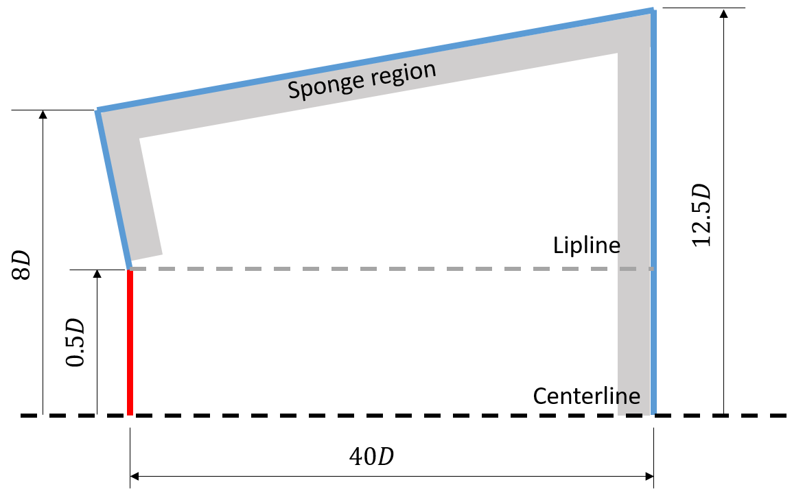
Figure 1: 2-D schematic representation of the computational domain used on the jet flow simulations.

The grid design attempts to capture the jet flow until a distance of $x/D=15$ from the inlet surface, indicated in red in Fig. 1. Then, the size of elements increases as an attempt to dissipate frequencies that could destabilize the simulation. Previous results [10] support the creation of mesh topology, indicating that a surface with one degree of opening angle would better represent the middle surface of the jet mixing layer. From this surface, two regions rise to increase the resolution of the domain. They have a geometrical stretching in the section $x/D=0$ to enable local refinement in the shear region of the flow and a uniform distribution in $x/D=15$. The internal section of the mixing layer connects to one hexahedral block that forms the core of the mesh. That hexahedral block has its dimensions defined to keep the size of the elements equal to the size of the last cells in the region of the mixing layer.

The grid refinement in the mixing layer is defined based on the literature [14, 5, 6, 7, 9]. The grid spacing in the radial and axial directions along the mixing layer is $\Delta y_{0}/D=0.001$ and $\Delta x_{0}/D=0.005$, respectively. The centerline presents 651 elements set in geometrical stretching distribution between $x/D=0$ and $x/D=15$. Each region of the mixing layer contains 50 cells, and the Azimuthal direction accommodates 180 elements evenly distributed. Figure 2a presents the radial mesh refinement in two different longitudinal positions, $x/D=0$ and $x/D=15$. Figure 2b illustrates the axial mesh refinement along the jet centerline and Fig. 3 exhibits a cutplane of the mesh generated for the current paper and the baseline line mesh used in previous work. The M-1 and M-2 grids have a total of 6.2 and 15.4 million cells, respectively, and they are created with the GMSH [28] mesh generator.

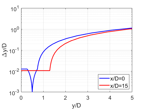
(a) Radial mesh refinement ($\Delta y/D$) in the longitudinal sections $x/D=0$ and $x/D=15$.

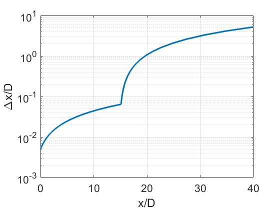
(b) Longitudinal mesh refinement ($\Delta x/D$) along the jet centerline.

Figure 2: Distribution of grid spacing indicating radial and longitudinal refinement for the M-2 mesh.

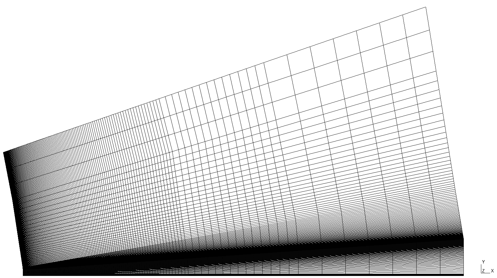
(a) M-1 mesh.

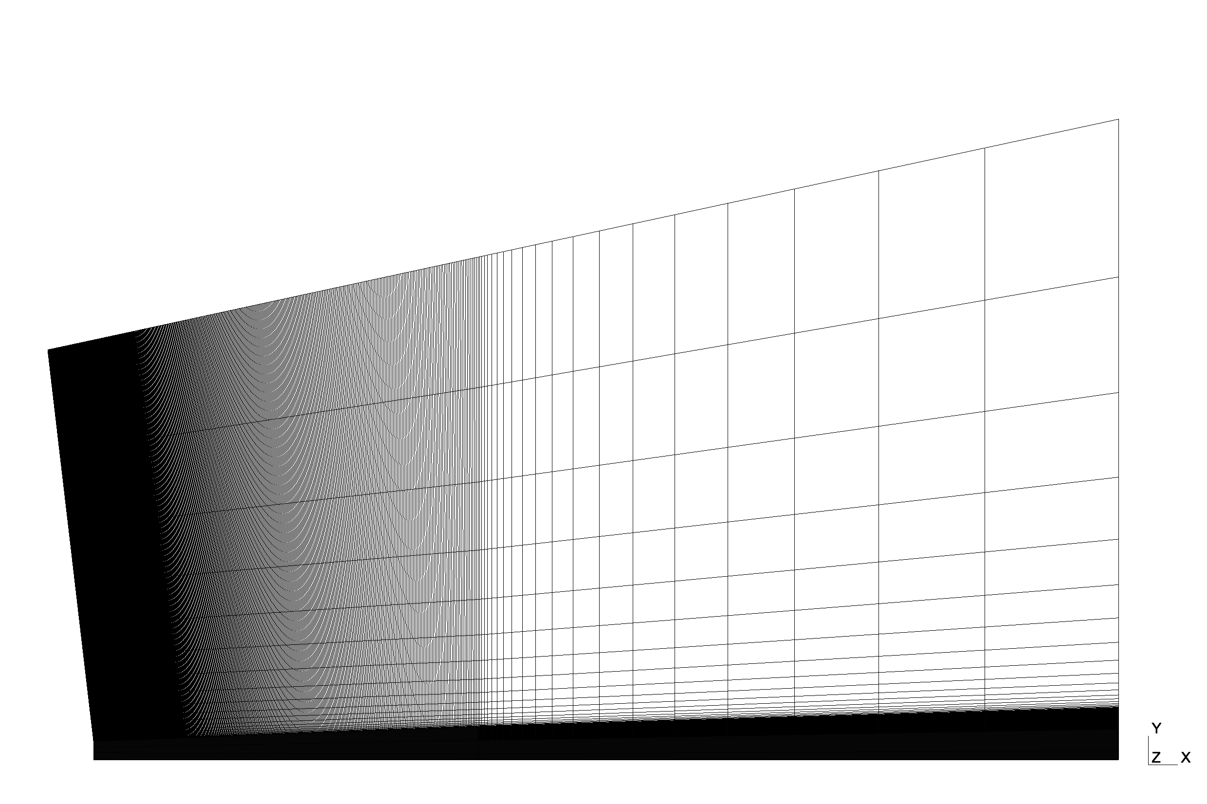
(b) M-2 mesh.

Figure 3: Visualization of the half-plane longitudinal cutplanes for the meshes used in the present work.

4.2 Boundary Conditions

Properties on the jet inflow, $(\cdot)_{jet}$, and farfield, $(\cdot)_{ff}$, surfaces are indicated in Fig. 1 in red and blue, respectively. A weakly enforced solution of a Riemann problem with a Dirichlet condition is enforced at the boundaries. The flow is characterized as perfectly expanded and isothermal, i.e. $p_{jet}/p_{ff}=T_{jet}/T_{ff}=1$, where $p$ stands for pressure and $T$ for temperature. The Mach number of the jet at the inlet is $M_{jet}=1.4$ and the Reynolds number based on the diameter of the nozzle is $Re_{jet}=1.58\times 10^{6}$. A small velocity component with $M_{ff}=0.01$ in the streamwise direction is imposed at the farfield to avoid numerical issues. A sponge zone [29] is employed around the farfield boundaries, the gray area presented in Fig. 1, to damp any oscillations that could be reflected back to the jet.

4.3 Simulation Settings and DOFs

The current work compares the effects of hp refinement using three different calculations: S1, S2, and S3. The first simulation uses the M-1 computational grid, while the other two computations apply the M-2 mesh. Both studies, S1 and S2, employ first-order polynomial reconstructions in order to achieve second-order accuracy in spatial discretization. Calculation S3 uses second-order polynomial reconstructions in order to achieve a third-order accurate spatial discretization. The simulations, therefore, consider from 50 to 410 million DOFs. Table 1 indicates the settings used the three numerical studies performed in the present effort.

Table 1: Summary of simulations settings.

Simulation	Meshes	Order of	DOF/cell	Cells	Total # of DOF
		Accuracy		($10^{6}$)	($10^{6}$)
S1	M-1	2nd order	8	$6.2$	$\approx 50$
S2	M-2	2nd order	8	$15.4$	$\approx 120$
S3	M-2	3rd order	27	$15.4$	$\approx 410$

4.4 Calculation of Statistical Properties

The simulation procedure involves three steps. The first one is to clean off the domain since the computation starts with a static flow initial condition. The simulations run three flow-through times (FTT) to develop the jet flow. One FTT is the time required for one particle with the jet velocity to cross the computational domain. In the sequence, the simulations run an additional three FTT to produce a statistically steady condition. Then, in the last step, data are collected for another three FTT to obtain the statistical properties of the flow.

The procedure for developing S3 simulation is slightly different. The simulation is a restart from the finished S2 calculation. The numerical framework FLEXI allows using one solution with different order of accuracy as initialization. Once the second-order solution was already available, its usage was a short come to initialize the S3 simulation. Hence, the S3 numerical study runs 0.5 FFT to allow the solution to adapt from second-order accuracy to third-order accuracy. Then it runs an additional 2 FTT to collect data. Different frequencies of data acquisition were employed in each simulation. The S1 case applies $160$ kHz, while S2 and S3 cases use $205$ and $225$ kHz, respectively.

The mean and the root mean square (RMS) fluctuations of properties of the flow are calculated along the centerline, lipline, and different domain surfaces in the streamwise direction. The centerline is defined as the line in the center of the geometry $y/D=0$, whereas the lipline is a surface parallel to the centerline and located at the nozzle diameter, $y/D=0.5$. The results from the lipline are an azimuthal mean from six equally spaced positions. The four surfaces in the streamwise positions are $x/D=2.5$, $x/D=5.0$, $x/D=10.0$, and $x/D=15.0$. Surface properties are averaged using six equally spaced positions in the azimuthal direction. Figure 4 illustrates a Mach number contours snapshot of the jet flow with the lines and surfaces of data extraction.

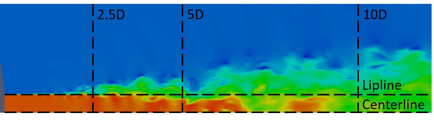
Figure 4: Snapshot of the jet simulation with the two longitudinal lines and three crossflow lines along which data is extracted. Mach number contours are shown.

5 Results

The results from S1, S2, and S3 simulations are presented in this section and compared to experimental data [19]. The focus of this work is to assess the resolution requirements for the correct prediction of supersonic jet flows. S1 and S2 calculations are performed with the same polynomial order of accuracy, while S3 simulation uses third-order accuracy polynomials. The S1 Numerical study is performed with mesh M-1, with $6.2\times 10^{6}$ elements, and S2 and S3 calculations are performed with mesh M-2, with $15.4\times 10^{6}$ elements. The simulations have approximately $50$, $120$, and $410$ million DOFs.

5.1 Velocity and Density Contours

Initially, the contours of the mean longitudinal velocity component, RMS of longitudinal velocity fluctuation, and mean density are presented for the three simulations. Figure 5 presents the contours of the mean longitudinal velocity component on a cut plane at $z/D=0$. The contours indicate qualitatively improvement in results when increasing the number of DOFs. One can notice the size of the jet core is bigger in Fig. 5c than in Figs. 5b and 5a. Moreover, the development of the mixing layer start closer to the jet inlet in S3 simulation than in S2 and S1 calculations. Furthermore, it is difficult to notice the existence of shock waves in Fig. 5a, which are more clearly visible in Figs. 5b and 5c.

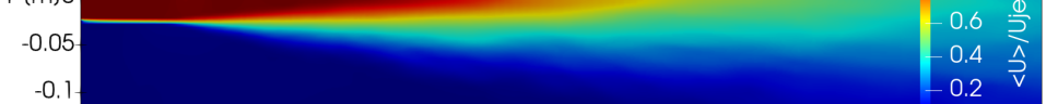
(a) S1 simulation.

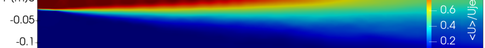
(b) S2 simulation.

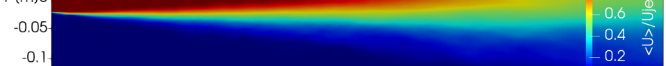
(c) S3 simulation.

Figure 5: Contours of mean longitudinal velocity component along cutplanes in $z/D=0$ for the three simulations performed.

Figure 6 presents the contours of RMS of longitudinal velocity fluctuations on a cut plane at $z/D=0$. One can notice the early development of the mixing layer when increasing the number of DOFs in the calculations. In Fig. 6c the increase in the RMS values for longitudinal velocity fluctuation occurs right after the boundary condition. The same physical phenomenon occurs farther when decreasing the simulation resolution, which is noticeable when comparing Fig.s 6b and 6a. The contours of RMS of longitudinal velocity fluctuation also show that the fluctuation levels get smaller with earlier development of the mixing layer. In Fig. 6c the region of high velocity fluctuation is thinner and presents smaller values than in Fig. 6b. In Fig. 6a, the region with a high level of velocity fluctuation is the largest, and it presents the highest values when compared to the other two results.

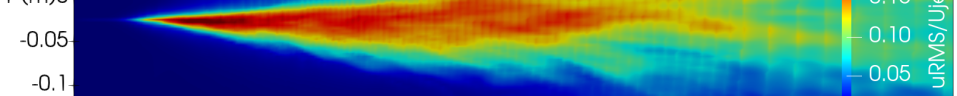
(a) S1 simulation.

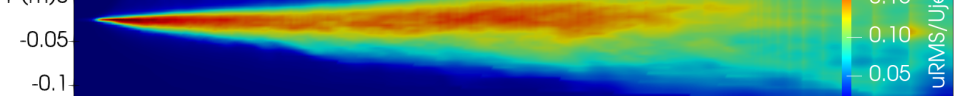
(b) S2 simulation.

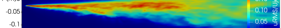
(c) S3 simulation.

Figure 6: Contours of RMS values of longitudinal velocity component fluctuations along cutplanes in $z/D=0$ for the three simulations performed.

The last contours presented in this section, Fig. 7, compare the mean density results from the three simulations on a cut plane at $z/D=0$. It is possible to observe that each simulation presents different characteristics. In Fig. 7a the shock waves are weak, being hardly visible with adequate range scales for all simulations. Moreover, one can notice a few shock waves and expansion waves reflections. The appearance of the first shock waves occurs far from the jet inlet boundary condition. Figure 7b presents a different behavior of the flow with shock waves and expansion waves significantly different from those observed in Fig. 7a. The first shock waves appear closer to the jet inlet boundary conditions, and they are visible, which indicates that they are significantly stronger than those from the S1 simulation. Another interesting observation is the number of shock waves and expansion waves reflection, which is much larger than the presented in Fig. 7a. The final density results are presented in Fig. 7c, which is the result from S3 simulation. It is possible to observe that the shock and expansion waves are better defined, presenting smaller thickness, which is also evidence of the improvements when increasing the number of DOFs in the simulation. When comparing the results from Fig. 7c with Fig. 7b, it is possible to observe that the intensity of the shock waves is stronger in S2 simulation than in S3, even with the larger thickness. This is in agreement with results presented in Figs. 5b and 5c, in which the shock waves from S2 calculation where more visible. The quantity of shock waves reflections in the S2 and S3 test cases are similar.

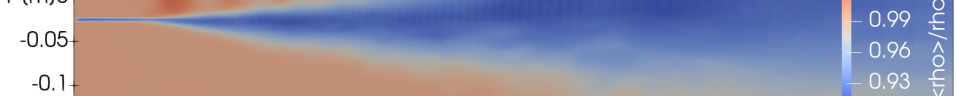
(a) S1 simulation.

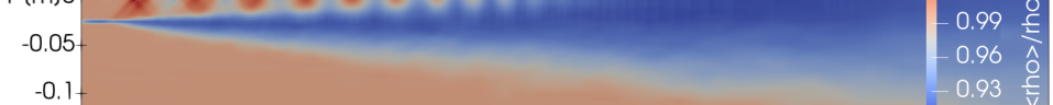
(b) S2 simulation.

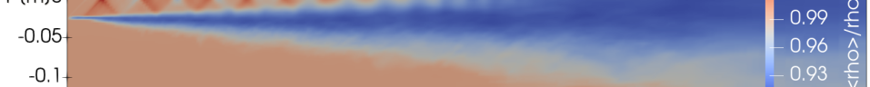
(c) S3 simulation.

Figure 7: Contours of mean density along cutplanes in $z/D=0$ for all three simulations.

5.2 Velocity Profiles

One can better understand the effects of the hp refinement on the numerical solution when comparing the results to the experimental data. Figure 8 presents the mean longitudinal velocity component and the RMS values of the velocity fluctuation distributions along the jet centerline ($y/D=0$) and the jet lipline ($y/D=0.5$). Analyzing the results presented in Fig. 8a, the improvement in the capacity to capture flow features when increasing the numerical resolution of the calculations is prominent. One can notice the numerical solution progression of the mean longitudinal velocity component towards the experimental data in Fig. 8a. The potential core is longer in S3 than in the other cases, which is presented in detail in Tab. 2. Moreover, the most refined numerical study presents the intensity of the shock waves and the slope of the decay of velocity comparable to the ones of the reference data. One can observe that the profiles calculated in S2 and S3 simulation are closer than the ones computed in S1 and S2, even with a higher ratio of degrees of freedom, $DOF_{S3}/DOF_{S2}\approx 3.42$ and $DOF_{S2}/DOF_{S1}\approx 2.4$. The slight improvement, even with a higher DOF ratio, can also indicate that the simulation S3 is very close to provide the converged solution for the chosen modeling approach.

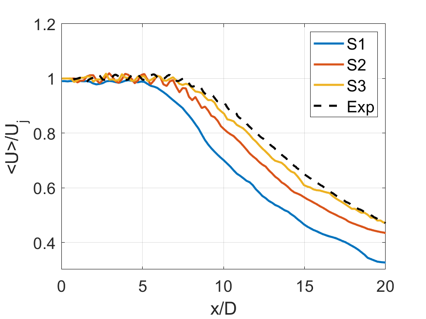
(a) Centerline, mean.

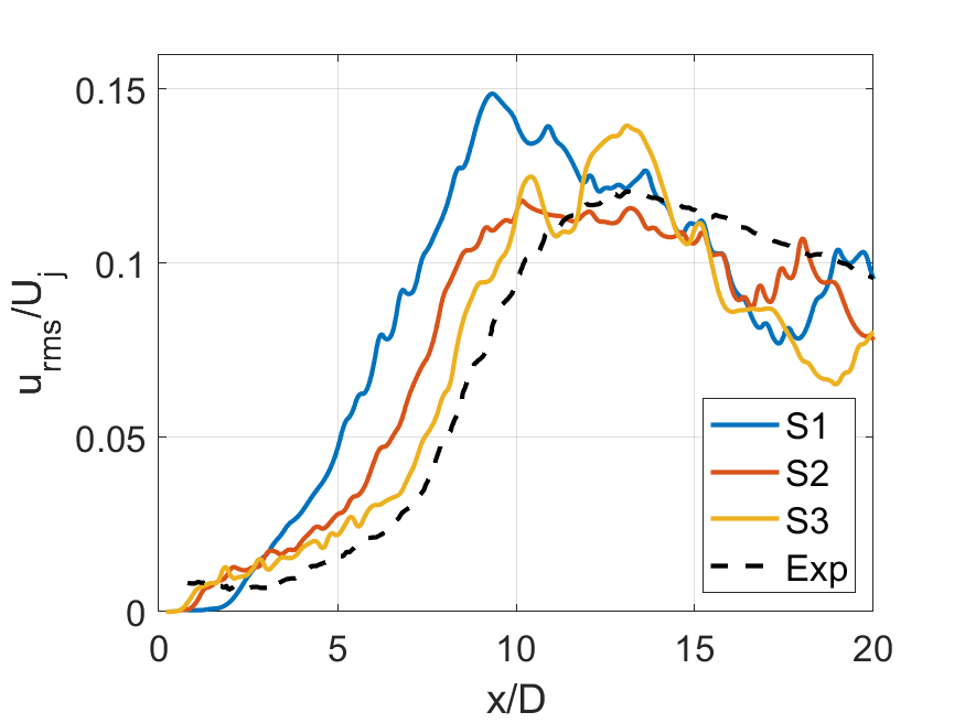
(b) Centerline, RMS values.

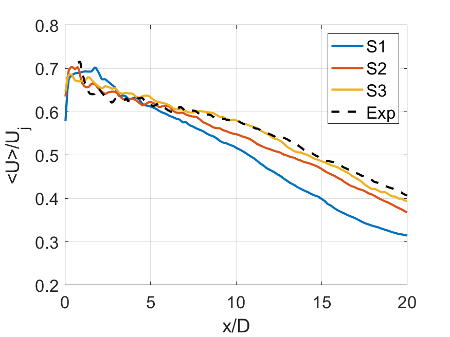
(c) Lipline, mean.

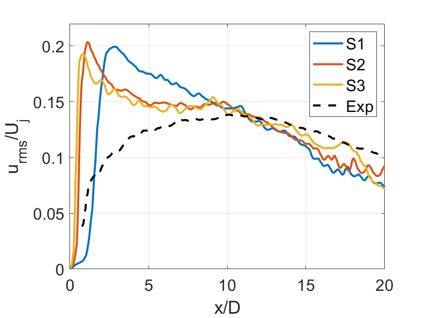
(d) Lipline, RMS values.

Figure 8: Results for the mean streamwise velocity component distributions (left) and RMS values of streamwise velocity component fluctuations (right) in the jet centerline, $y/D=0$ (top), and lipline, $y/D=0.5$ (bottom).

Table 2: Summary of potential core length for all simulations.

Simulation	Potential core	Error to
	length ($x/D$)	experimental data ($\%$)
S1	6.3	30.0
S2	7.8	13.3
S3	8.5	5.5

The results presented in Fig. 8b agree well with the results of Fig. 8a. The increase in the simulation resolution improves the calculation of RMS velocity fluctuation towards the experimental data. Analyzing the results close to the jet inlet, the increase in the velocity fluctuation occurs further upstream in S3 simulation, which is in agreement with the contours in Figs. 5 where the shock waves of S3 numerical study appear closer to jet inlet when compared to the S2 and S1 calculations. However, even with an early increase in the fluctuation levels in S3 computations, the slope of its profile in Fig. 8b is smoother and closer to the reference than the one calculated in S2 and S1 numerical studies. In the same image, S3 simulation presents two peaks of velocity fluctuation, with the second one close to the peak indicated in the experiment. However, its RMS fluctuations are higher than experimental data and S2 simulation solution. The presence of small values of velocity fluctuation close to the jet inlet could be related to imposed jet entrance boundary conditions.

Figures 8c and 8d illustrate the profiles of mean and RMS fluctuations of the longitudinal velocity component along the lipline, respectively. One can notice the improvements in the simulation resolution with S3 and S2 simulations providing mean profiles closer to the experimental one than the results from the S1 calculation. The mean velocity oscillations in the vicinity of the inlet jet may be correlated with shock waves. They are also present in the experimental profile along the lipline. The S1 and S2 simulations present an early reduction of mean velocity when comparing to the reference profile. The most refined calculation has a mean velocity profile in good agreement with the experimental data along the lipline. Such behavior is also noticeable along the centerline. The calculations performed in the present paper have generated fluctuation profiles of the longitudinal velocity fluctuation along the lipline, Fig. 8d, that indicate a different trend from what is stated in Figs. 8a to 8c. One can notice that, when increasing the simulation resolution, the peak of velocity fluctuation moves towards the jet inlet, at $x/D=2.5$ for S1 simulation and $\approx x/D=1$ for S2 and S3 calculations. This outcome is present in the contours indicated in Fig. 5, where the initial spreading of the mixing layer in S2 and S3 simulations starts earlier than in the S1 calculation. Such behavior is different from the experimental RMS profiles along the lipline in which the increase in the velocity fluctuation occurs slowly before reaching a plateau between $x/D=5$ to $x/D=15$. Using a flat hat velocity profile at the jet entrance for the numerical calculations can explain the divergence between the fluctuations obtained from the numerical approach and the experiments near the inlet domain. Such boundary condition neglects the turbulent boundary layer effects carried from the nozzle to the jet flow.

Figure 9 displays different statistical properties of the flow in four streamwise positions, $x/D=2.5$, $x/D=5$, $x/D=10$ and $x/D=15$. Figures 9a to 9d present the mean longitudinal velocity component, Figs. 9e to 9h illustrate the RMS of the longitudinal velocity fluctuation, Figs. 9i to 9l introduces the RMS of the radial velocity fluctuation, and Figs. 9m to 9p indicate the mean shear stress tensor.

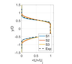
(a) $x/D=2.5$

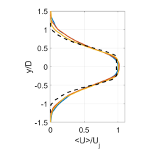
(b) $x/D=5$

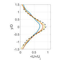
(c) $x/D=10$

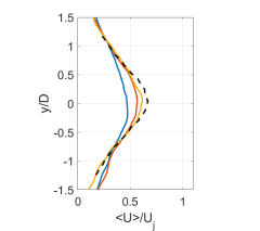
(d) $x/D=15$

(e) $x/D=2.5$

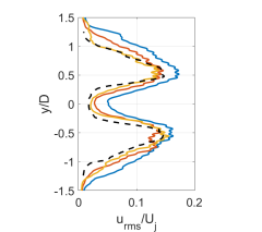
(f) $x/D=5$

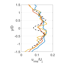
(g) $x/D=10$

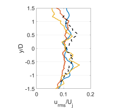
(h) $x/D=15$

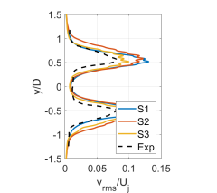
(i) $x/D=2.5$

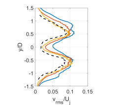
(j) $x/D=5$

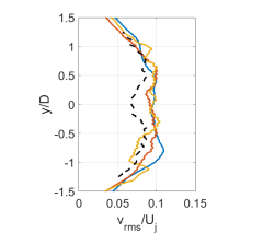
(k) $x/D=10$

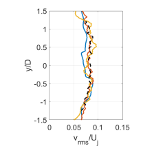
(l) $x/D=15$

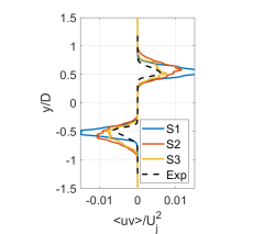
(m) $x/D=2.5$

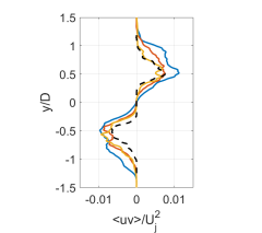
(n) $x/D=5$

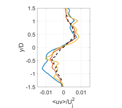
(o) $x/D=10$

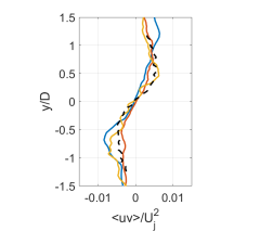
(p) $x/D=15$

Figure 9: Profiles of mean streamwise velocity component, RMS of streamwise velocity fluctuation, RMS of radial velocity fluctuation, and mean shear-stress tensor component (from top to bottom) at four streamwise positions $x/D=2.5$, $x/D=5$, $x/D=10$ and $x/D=15$ (from left to right).

The first set of results, in Figs. 9a to 9d, explicit some aspects of the numerical results not investigated by the comparison of 2-D field of properties. In the first longitudinal position, Fig. 9a, S1 calculations generated mean profiles that are in better agreement with the experimental data than the ones from S2 and S3 numerical studies, which indicate a larger spreading of velocity at this position. The early development of the mixing layer from S2 and S3 simulations reinforces the influence of the choice of boundary conditions imposed. Analyzing the profiles from downstream positions, Figs. 9b to 9d, it is possible to verify the large spreading of velocity from the S1 simulation, with a reduction of longitudinal velocity in the jet centerline when compared to the other numerical solutions. Calculations with higher resolution can better capture the experimental trends, with the simulation S3 getting closer to experimental data.

The profiles of RMS values of streamwise velocity fluctuation are indicated in Figs. 9e to 9h. The numerical results at $x/D=2.5$ present a similar profile to the one from the reference. However, the peaks generated by the calculations are higher than the experimental ones, with the results from the S3 simulation being the closest to experimental data. The same conclusion can be drawn for $x/D=5.0$, Fig. 9f. In Figs. 9g and 9h, the all numerical results present a shape similar to experimental data, with a nearly constant value of velocity fluctuation. In Fig. 9g the experimental data still present a small level of fluctuation close to the centerline, which is not seen in the numerical profiles.

Profiles of RMS values of radial velocity component fluctuation are presented in Figs. 9i to 9l. In the first two longitudinal positions, Figs. 9i and 9j, the numerical results present a larger peak of fluctuation than the one from the experimental data, with the profiles from the S3 simulation getting closer to reference. In Figs. 9k and 9l the RMS profiles from the calculations are very similar, with the centerline of the experimental data presenting small values of fluctuation in Fig. 9k.

Mean shear-stress tensor component profiles are presented in Figs. 9m to 9p. In the first two positions, $x/D=0.5$ and $x/D=2.5$, the peak of the shear-stress tensor from numerical calculations is larger than the experimental one. Moreover, the peak region is wider than the one observed in the experiments. In Fig. 9n the peaks are still larger than those observed in the reference. The differences between the simulations are smaller and closer to experimental data. However, the region of the peaks is still wider than the one visualized in the experimental data. In Figs. 9o and 9p, the differences between numerical results and the experimental data are reduced, and once more, all profiles are nearly matching.

5.3 Summary of Discussions

Results from the S2 simulation present significant improvements when compared to the solution from the S1 calculation. The increase in polynomial order of accuracy in the S3 study brings the results to a good agreement with the reference experimental data. The most significant point that does not present improvements when increasing the discretization resolution is related to the mean and fluctuating longitudinal velocity close to jet lipline, Figs. 8c and8d. Grid refinement yields a velocity fluctuation peak that occurs closer to the jet inlet when compared to the experimental data. This behavior may be related to the hypothesis used to impose the inlet boundary condition, which neglects the effects of the jet boundary layer and leads to a not realistic turbulence transition in the vicinity of the nozzle.

The current work provides intel on the resolution requirements to perform large-eddy simulations of supersonic jet flows. The next step concerns the exploration of alternatives to improve the jet simulation in the lipline close to the jet inlet condition. A solution to improve the simulation in this region is a better characterization of the flow leaving the nozzle. The choice of a uniform velocity profile is preliminary, and it does not represent the physics of the flow. The continuity of the work will focus on options to produce an experiment-like condition in the jet inlet condition.

6 Concluding Remarks

The current work assesses the effects of mesh and polynomial (hp) refinement using a nodal discontinuous Galerkin methodology to evaluate the resolution requirements for large eddy simulations of compressible jet flows. The problem of interest is a perfectly expanded supersonic jet flow with a Mach number of $1.4$ and Reynolds number based on the jet exit diameter of $1.58\times 10^{6}$. Initially, a mesh with $6.2\times 10^{6}$ elements is used with interpolation polynomials that yield second-order spatial accuracy, in order to produce a starting point for the comparisons. Such calculations use, therefore, the equivalent to approximately $50\times 10^{6}$ degrees of freedom (DOFs). Afterwards, a new mesh is developed with some topological improvements and additional refinement, leading to $15.4\times 10^{6}$ elements. The new mesh is applied in simulations using second-order and third-order spatial accuracy, resulting in $120\times 10^{6}$ and $410\times 10^{6}$ DOFs, respectively. The results for the simulations are compared to experimental data.

The paper initially investigates the contours of mean velocity, mean pressure, and velocity fluctuations. The comparison indicates that the mesh/polynomial refinement improves the jet calculations by enhancing the prediction of the mixing layer and of the series of shock and expansion waves in the jet core. Therefore, as one should expect, more refined computations lead to an improved ability to predict flow features, as one can see in the present paper by the comparison of the numerical solutions and the experimental data. Therefore, it is correct to state that the present paper indicates mesh and discretization parameters for LES-based calculations, using a nodal discontinuous Galerkin formulation, that provide supersonic jet flow results in good agreement with experiments.

One important aspect that becomes clear in the present calculation results is that the jet inlet boundary condition, used in the current work, has a significant impact on the ability of representing the very early stages of jet mixing. In particular, this observation becomes evident by looking at the behavior of RMS values of fluctuating properties near the jet exit, along the jet lipline. All three simulations have failed to capture the correct mixing behavior, as evidenced by the comparison with the experimental data. Moreover, the increased numerical resolution, although providing much better comparisons for the overall solution, does not improve the behavior of fluctuating properties near the jet exit. Hence, the continuation of the present effort will address possible improvements in the jet inlet boundary conditions.

References

- Brès and Lele [2019] Brès, G. A., and Lele, S. K., “Modelling of Jet Noise: A Perspective from Large-Eddy Simulations,” Philosophical Transactions of the Royal Society A, Vol. 377, No. 2159, 2019, p. 20190081.
- Kumar and Mahesh [2017] Kumar, P., and Mahesh, K., “Large Eddy Simulation of Propeller Wake Instabilities,” Journal of Fluid Mechanics, Vol. 814, 2017, p. 361–396. 10.1017/jfm.2017.20.
- Ghate et al. [2021] Ghate, A. S., Gaetan, K. K., Stich, G.-D., Oliver, M. B., Jeffrey, A. H., and Kiris, C. C., “Transonic Lift and Drag Predictions Using Wall-Modelled Large Eddy Simulations,” AIAA Paper No. 2021-1439, AIAA Scitech 2021 Forum, Virtual event, 2021.
- Masoudi et al. [2021] Masoudi, E., Gan, L., and Sims-Williams, D., “Large Eddy Simulation of Incident Flows Around Polygonal Cylinders,” Physics of Fluids, Vol. 33, No. 10, 2021, p. 105112.
- Bogey and Marsden [2016] Bogey, C., and Marsden, O., “Simulations of Initially Highly Disturbed Jets with Experiment-Like Exit Boundary Layers,” AIAA Journal, Vol. 54, No. 4, 2016.
- Brès et al. [2017] Brès, G. A., Ham, F. E., Nichols, J. W., and Lele, S. K., “Unstructured Large-Eddy Simulations of Supersonic Jets,” AIAA Journal, Vol. 55, No. 4, 2017.
- DeBonis [2017] DeBonis, J. R., “Prediction of Turbulent Temperature Fluctuations in Hot Jets,” AIAA Paper No. 2017-0610, Proceedings of the 23th AIAA Computational Fluid Dynamics Conference, Denver, CO, 2017.
- Abreu et al. [2021] Abreu, D. F., Junqueira-Junior, C., Dauricio, E. T. V., and Azevedo, J. L. F., “A Comparison of Low and High-Order Methods for the Simulation of Supersonic Jet Flows,” Proceedings of the 26th ABCM International Congress of Mechanical Engineering, COBEM Paper No. 2021-0388, Florianópolis, Santa Catarina, Brazil, 2021.
- Junqueira-Junior et al. [2018] Junqueira-Junior, C., Yamouni, S., Azevedo, J. L. F., and Wolf, W. R., “Influence of Different Subgrid-Scale Models in Low-Order LES of Supersonic Jet Flows,” Journal of the Brazilian Society of Mechanical Sciences and Engineering, Vol. 40, 2018, pp. 258.1–258.29.
- Junqueira-Junior et al. [2020] Junqueira-Junior, C., Azevedo, J. L. F., Panetta, J., Wolf, W. R., and Yamouni, S., “On the Scalability of CFD Tool for Supersonic Jet Flow Configurations,” Parallel Computing, Vol. 93, 2020, pp. 102620.1–102620.13.
- Kopriva and Gassner [2010] Kopriva, D. A., and Gassner, G., “On the Quadrature and Weak Form Choices in Collocation Type Discontinuous Galerkin Spectral Element Methods,” Journal of Scientific Computing, Vol. 44, 2010, pp. 136–155.
- Hindenlang et al. [2012] Hindenlang, F., Gassner, G. J., Altmann, C., Beck, A., Staudenmaier, M., and Munz, C.-D., “Explicit Discontinuous Galerkin Methods for Unsteady Problems,” Computer & Fluids, Vol. 61, 2012, pp. 86–93.
- Krais et al. [2021] Krais, N., Beck, A., Bolemann, T., Frank, H., Flad, D., Gassner, G., Hindenlang, F., Hoffmann, M., Kuhn, T., Sonntag, M., and Munz, C.-D., “FLEXI: A High Order Discontinuous Galerkin Framework for Hyperbolic–Parabolic Conservation Laws,” Computers and Mathematics with Applications, Vol. 81, 2021, pp. 186–219.
- Bogey and Bailly [2010] Bogey, C., and Bailly, C., “Influence of Nozzle-Exit Boundary-Layer Conditions on the Flow and Acoustic Fields of Initially Laminar Jets,” Journal of Fluid Mechanics, Vol. 663, 2010, pp. 507–538.
- Mendez et al. [2012] Mendez, S., Shoeybi, M., Sharma, A., Ham, F. E., Lele, S. K., and Moin, P., “Large-Eddy Simulations of Perfectly Expanded Supersonic Jets Using an Unstructured Solver,” AIAA Journal, Vol. 50, No. 5, 2012. https://doi.org/10.2514/1.J051211.
- Brès et al. [2018] Brès, G. A., Jordan, P., Jaunet, V., Rallic, M. L., Cavalieri, A. V. G., Towne, A., Lele, S. K., Colonius, T., and Schmidt, O. T., “Importance of the Nozzle-Exit Boundary-Layer State in Subsonic Turbulent Jets,” Journal of Fluid Mechanics, Vol. 851, 2018, pp. 83–124.
- Shen and Miller [2019] Shen, W., and Miller, S. A. E., “Validation of a High-Order Large Eddy Simulation Solver for Acoustic Prediction of Supersonic Jet Flow,” Journal of Theoretical and Computational Acoustics, Vol. 1950023, 2019.
- Corrigan et al. [2018] Corrigan, A., Kercher, A., Liu, J., and Kailasanath, K., “Jet Noise Simulation using a Higher-Order Discontinuous Galerkin Method,” AIAA Paper No. 2018-1247, Proceedings of the 2018 AIAA Aerospace Sciences Meeting, Kissimmee, FL, 2018.
- Bridges and Wernet [2008] Bridges, J., and Wernet, M. P., “Turbulence Associated with Broadband Shock Noise in Hot Jets,” AIAA Paper No. 2008-2834, 29th AIAA Aeroacoustics Conference, Vancouver, British Columbia, Canada, 2008.
- Vreman [1995] Vreman, A. W., “Direct and Large Eddy Simulation of the Compressible Turbulent Mixing Layer,” Ph.D. thesis, University of Twente, Twente, Netherlands, 1995.
- Smagorinsky [1964] Smagorinsky, J., “General Circulation Experiments with the Primitive Equations: I. The Basic Experiment,” Monthly Weather Review, Vol. 93, No. 3, 1964, pp. 99–164.
- Pirozzoli [2011] Pirozzoli, S., “Numerical Methods for High-Speed Flows,” Annual Review of Fluid Mechanics, Vol. 43, 2011, pp. 163–194.
- Gassner et al. [2016] Gassner, G. J., Winters, A. R., and Kopriva, D. A., “Split Form Nodal Discontinuous Galerkin Schemes with Summation-by-Parts Property for the Compressible Euler Equations,” Journal of Computational Physics, Vol. 327, 2016, pp. 39–66.
- Harten and Hyman [1983] Harten, A., and Hyman, J. M., “Self Adjusting Grid Methods for one Dimensional Hyperbolic Conservation Laws,” Journal of Computational Physics, Vol. 50, 1983, pp. 253–269.
- Bassi and Rebay [1997] Bassi, F., and Rebay, S., “A High-Order Accurate Discontinuous Finite Element Method for the Numerical Solution of the Compressible Navier-Stokes Equations,” Journal of Computational Physics, Vol. 131, 1997, pp. 267–279.
- Carpenter and Kennedy [1994] Carpenter, M. H., and Kennedy, C. A., “Fourt-Order 2N-Storage Runge-Kutta Schemes,” Tech. Rep. NASA-TM-109112, NASA Langley Research Center, 1994.
- Sonntag and Munz [2017] Sonntag, M., and Munz, C.-D., “Efficient Parallelization of a Shock Capturing for Discontinuous Galerkin Methods using Finite Volume Sub-cells,” Journal of Scientific Computing, Vol. 70, 2017, pp. 1262–1289.
- Geuzaine and Remacle [2009] Geuzaine, C., and Remacle, J. F., “GMSH: A Three-Dimensional Finite Element Mesh Generator with Built-in Pre- and Post-Processing Facilities,” International Journal for Numerical Methods in Engineering, Vol. 79, No. 11, 2009, pp. 1309–1331.
- Flad et al. [2014] Flad, D. G., Frank, H. M., Beck, A. D., and Munz, C.-D., “A Discontinuous Galerkin Spectral Element Method for the Direct Numerical Simulation of Aeroacoustics,” AIAA Paper No. 2014-2740, Proceedings of the 20th AIAA/CEAS Aeroacoustics Conference, Atlanta, GA, 2014.