Universal to Non-Universal Transition of the statistics of Rare Events During the Spread of Random Walks

Abstract

Particle hopping is a common feature in heterogeneous media. We explore such motion by using the widely applicable formalism of the continuous time random walk and focus on the statistics of rare events. Numerous experiments have shown that the decay of the positional probability density function $P(X,t)$, describing the statistics of rare events, exhibits universal exponential decay. We show that such universality ceases to exist once the threshold of exponential distribution of particle hops is crossed. While the mean hop is not diverging and can attain a finite value; the transition itself is critical. The exponential universality of rare events arises due to the contribution of all the different states occupied during the process. Once the reported threshold is crossed, a single large event determines the statistics. In this realm, the big jump principle replaces the large deviation principle, and the spatial part of the decay is unaffected by the temporal properties of rare events.

According to Wikipedia, ”Rare or extreme events are events that occur with low frequency, and often refers to infrequent events that have widespread impact and might destabilize systems”. Notable examples of rare events include the stock market crash Amihud et al. (1990), earthquakes Lomnitz (1966) and cyclones Leckebusch and Ulbrich (2004). The most recent on the list is the 2020 pandemic, which brought the whole world to a standstill. The frequency and the scale of rare events in each field are very important. If the rare events are not ”too rare” and large enough, then the usual statistical behavior is completely dictated by such rare events. A perfect example of situations when rare events fundamentally modify the nature of a physical process is sub-diffusion Metzler and Klafter (2000); Weiss and Rubin (1983); Alexander et al. (1981); Havlin and Ben-Avraham (1987); Isichenko (1992); Shlesinger et al. (1993); Haus and Kehr (1987). While for normal diffusion, the mean squared displacement (MSD) of a tracked particle grows linearly with time, for sub-diffusion, the MSD grows in a non-linear fashion, i.e. $\langle X^{2}\rangle\sim t^{\alpha}$, while $0<\alpha<1$. Sub-diffusion generally occurs when there are long time or space correlations present. One of the sources for such correlations can appear in the form of an extremely long sojourn times, when the tracked particle is trapped in a specific region in space Scher et al. (1991). When sub-diffusion occurs in amorphous materials like glasses Binder and Young (1986) or living cells Manzo et al. (2015); Granéli et al. (2006); Wang et al. (2006), it is quite common to observe trajectories that are dominated by several (and sometimes even one) very long trapping events Jeon et al. (2011).

In many cases, the appearance of sub-diffusion is accompanied by unusual physical phenomena: aging Bouchaud (1992); Akimoto et al. (2016); Barkai and Cheng (2003), weak ergodicity breaking Bouchaud (1992); Rebenshtok and Barkai (2007); Bel and Barkai (2005) and non-self-averaging Bouchaud (1992); Burov and Barkai (2007); Pronin (2022); Sabhapandit (2011); Burov (2017); Shafir and Burov (2022). Studies of theoretical models where trapping is present, like the continuous time random walk (CTRW) Klafter and Sokolov (2011) and the quenched trap model (QTM) Bouchaud and Georges (1990) show that there is a critical transition to sub-diffusion, aging, and non-ergodic behavior, when the mean trapping time is diverging. This transition is also accompanied by a transformation of the positional probability density function (PDF). The universal Gaussian center of the positional PDF turns into an $\alpha$-stable Lévy type Uchaikin (2003); Garoni and Frankel (2002), i.e. shape that depends on a specific parameter $\alpha$ that determines the trapping times. This transition between a universal PDF that is determined by an accumulation of many events, and a non-universal PDF that follows the properties of one single rare event is a key feature associated with the the appearance of new physical phenomena. Can transitions from universal to non-universal PDFs symbolize an underlying phase transition that might lead to uncovered surprising physics, like in the case of sub-diffusion? What are the properties of single rare events that can cause such a critical transition in behavior? In this work, we focus on the appearance of the universal to the non-universal transition of a positional PDF that, unlike the case of sub-diffusion, appears for large positions $|X|$ (the tails of the PDF).

Recently, in a huge number of experiments, exponential (and not Gaussian) decay of the PDF for large $|X|$ was spotted. Such decay of the PDF is termed Laplace tails Chechkin et al. (2017). Notable examples include colloidal beads in heterogeneous optical force field Pastore et al. (2021), zooplanktons under crowding Uttieri et al. (2021), glass-forming liquids Rusciano et al. (2022), nanoparticles in polymer melts Xue et al. (2016), motion of particles at liquid-solid interface Wang et al. (2017), particle displacements close to glass and jamming transitions Chaudhuri et al. (2007, 2008) etc. In Wang et al. (2012) it was suggested that there might exist a universal convergence to the Laplace tails. Indeed it was proven, by exploiting the CTRW model that for a wide range of processes, the tails of the PDF are determined by the accumulation of many events and follow exponential decay (up to logarithmic corrections) Barkai and Burov (2020); Wang et al. (2020a); Pacheco-Pozo and Sokolov (2021). So by following the presented discussion, we ask: Is there a transition from universal Laplace tails to non-universal and process-specific tails? And if so, is it accompanied by a critical transition like the diffusion to subdiffusion transition? Are the tails of a PDF determined by one occurrence of one single event Foss et al. (2013); Embrechts et al. (2013); Kutner (2002); De Mulatier et al. (2013); Majumdar et al. (2005) or they represent an accumulation of many realizations of not-so-large but more frequent events Hollander (2000); Ellis (1999); Dembo and Zeitouni (2009); Nickelsen and Touchette (2018); Touchette (2009)?

Similar to the case of subdiffusion to diffusion transition, we use the celebrated CTRW model, originally exploited for explaining motion in amorphous materials Binder and Young (1986); Manzo et al. (2015); Granéli et al. (2006); Wang et al. (2006) and exponential decay of tails Chechkin et al. (2017). In this model, a particle performs random jumps in space and waits for a random amount of time between every two jumps. All the jumps and waiting times are independent and identically distributed (IID) random variables. The distribution of a jump $x$ is given by $f(x)$, while each waiting time $\tau$ has a distribution $\psi(\tau)$. The position of the process $X$ at time $t$ is determined by the random number of jumps $N_{t}$ performed by time $t$, i.e. $X=x_{1}+\dots+x_{N_{t}}$ where $x_{i}$, is the size of a single jump. The positional PDF $P(X,t)$ is readily obtained in terms of the subordination equation by conditioning on the number of jumps $N$, He et al. (2008); Magdziarz et al. (2008); Bouchaud and Georges (1990); Metzler and Klafter (2000)

$$P(X,t)=\sum^{\infty}_{N=0}P_{N}(X)Q_{t}(N)$$ (1)

where $P_{N}(X)$ is the distribution of $X$ for a given $N$($=N_{t}$ for a fixed measurement time $t$) and $Q_{t}(N)$ is the distribution of the number of jumps up to time $t$. The mentioned phenomena, like anomalous transport and aging, appear for CTRWs with $\psi(\tau)\sim\tau^{-1-\alpha}$ ($\tau\to\infty$) when $\alpha<1$. For such $\psi(\tau)$, the sum $\tau_{1}+\cdots+\tau_{N_{t}}$ is dominated (in the $t\to\infty$ limit) by the maximal summand Derrida (1997), as can be observed from the behavior of

$$\phi_{\alpha}(t)=\Big{\langle}\frac{\text{max}\{\tau_{1},...,\tau_{N_{t}}\}}{\sum^{N_{t}}_{i=1}\tau_{i}}\Big{\rangle}$$ (2)

for large $t$. While the maxima of a set of random variables has been extensively studied Majumdar (2010); Mounaix et al. (2018); Mori et al. (2020); Höll and Barkai (2021), the definition of $\phi_{\alpha}(t)$ has the advantage that it ranges from infinitesimal to finite values. This makes it appropriate as an order parameter. We see in Fig. 1 (inset) that $\phi_{\alpha}(t)$ saturates to a finite value for $\alpha=0.5,~{}0.8,~{}0.9$ while for $\alpha=1.1,~{}1.2,~{}1.5$ exhibits a decaying behavior at large times. This difference in the properties of $\phi_{\alpha}(t)$ follows from the fact that for $\alpha<1,~{}\langle\tau\rangle=\int^{\infty}_{0}d\tau~{}\tau\psi(\tau)\to\infty$, while it is finite for $\alpha>1$. This implies that as we move from $\alpha>1$ to $\alpha<1$, the rare fluctuations in the sequence of waiting times $\{\tau_{1},...,\tau_{N_{t}}\}$ exhibit qualitatively different behaviors. Consequently, the thermodynamic limit in which the system behaves extensively (all waiting times $\tau_{i}$ are of the same order of magnitude) ceases to exist for $\alpha<1$. Can we see similar behavior if we focus on spatial fluctuations? This question comes up naturally once we realize that the system has access to the entire phase space in the thermodynamic limit. The phase space can be swept by focusing on large spatial fluctuations without going to the $t\to\infty$ limit. This means we take the large $|X|$ limit and expect the system to visit many states during its evolution.

Motivated by this, let us look at a CTRW described by Eq. (1) with jumps following $f(x)\sim e^{-|x|^{\beta}}$ with $\beta>0$ Nardon and Pianca (2009). In analogy with $\phi_{\alpha}(t)$ let us define

$$F_{\beta}(X)=\Big{\langle}\frac{\text{max}\{|x_{1}|,...,|x_{N_{t}}|\}}{\sum^{N_{t}}_{i=1}|x_{i}|}\Big{\rangle}.$$ (3)

We see in Fig. 1 that even for a well behaved $\psi(\tau)$ like the exponential

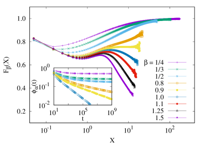
Figure 1: $F_{\beta}(X)$ for a CTRW with jumps $x\sim f(x)$ with mean zero and variance one as a function of $\beta$. The waiting time distribution $\psi(\tau)=e^{-\tau}$ and the measurement is done at $t=0.6$ for trajectories reaching a position $\pm X$. Inset shows the behavior of $\phi_{\alpha}(t)$ for $\psi(\tau)\sim\tau^{-1-\alpha}$ for large $\tau$ and $\alpha=0.5,0.8,0.9,1.1,1.2,1.5$ from top to bottom.

distribution, $\lim_{|X|\to\infty}F_{\beta}(X)$ decreases monotonically for $\beta\geq 1$ and takes a finite value for trajectories with $\beta<1$. In other words,

$$\lim_{|X|\to\infty}F_{\beta}(X)=\begin{cases}0,~{}~{}\beta\geq 1\\ c_{\beta},~{}~{}\beta<1\end{cases}$$ (4)

where $c_{\beta}$ is a nonzero constant that depends on $\beta$. Although $c_{\beta}$ is seen to approach unity for $\beta=1/2$ and lower values, $\beta=0.9$ seems to saturate to a value less than one. While the transition of $\phi_{\alpha}(t)$ is driven by the divergence of the mean waiting time $\langle\tau\rangle$, this is not the case for the transition of $F_{\beta}(X)$. All the moments $\langle x^{n}\rangle$ are finite for $\beta<1$. Nevertheless, the effective behavior of $\lim_{t\to\infty}\phi_{\alpha}(t)$ and $\lim_{|X|\to\infty}F_{\beta}(X)$ is similar. As a function of the parameters $\alpha$/$\beta$, there is a transition from a state defined by the accumulation of many events to a state dominated by a single large event.

At this point, it is worth noticing that the role played by $\phi_{\alpha}(t)$ for describing temporal fluctuations is taken over by $F_{\beta}(X)$ for spatial fluctuations. While the emergence of a non-Gaussian center accompanying the transition of $\phi_{\alpha}(t)$ is well understood Uchaikin (2003); Garoni and Frankel (2002) the corresponding behavior of $P(X,t)$ accompanying the transition of $F_{\beta}(X)$ is not known. It was shown in Ref. Barkai and Burov (2020) that $P(X,t)$ exhibits universal tails exhibiting exponential decay for $\beta>1$ and $\psi(\tau)$ analytic near $\tau=0$. Furthermore, just like $\phi_{\alpha}(t)\to 0$ marks the emergence of a universal Gaussian center following the central limit theorem, $F_{\beta}(X)\to 0$ at $|X|\to\infty$ characterizes the universal exponential tails of $P(X,t)$ Barkai and Burov (2020). On the other hand, a finite value of $\phi_{\alpha}(t)$ for $\alpha<1$ is reminiscent of the Lévy stable PDF and is a reminder of the dynamical phase transition (DPT) Nyawo and Touchette (2017, 2018); Garrahan et al. (2007); Jack and Sollich (2013) characterized solely by the rare fluctuations, but in the temporal domain. Does it mean we can see a similar DPT at finite times if we focus on the tails of $P(X,t)$? We now answer this question by exploring the case of $\beta\leq 1$.

For $\beta=1$, the jumps follow Laplace distribution, that is, $f(x)=\frac{a}{2}\exp(-a|x|)$. This implies that the characteristic function of a single jump, defined as the Fourier transform $\hat{\lambda}(k)=\int^{\infty}_{-\infty}dx~{}e^{ikx}f(x)=\frac{a^{2}}{a^{2}+k^{2}}$ Klafter and Sokolov (2011). Unlike the case for $\beta>1$, $\hat{\lambda}(k)$ for $\beta=1$ has poles in the complex plane. Furthermore, since the jumps are IID, the distribution of a sum of $N$ jumps in Fourier space is $\hat{\lambda}^{N}(k)$ and inverting it via contour integration Watson (1922) we find that the distribution of position $X$ after $N$ jumps is Gradshteyn and Ryzhik (2014)

$$P_{N}(X) =\frac{ae^{-a|X|}}{2^{2N-1}\Gamma(N)}\sum^{N-1}_{m=0}\frac{(2N-m-2)!}{m!(N-m-1)!}(2a|X|)^{m}$$

$$\approx\frac{ae^{-a|X|}}{2^{2N}\Gamma(N)}\int^{N}_{0}dm~{}\exp[K(N,m)]$$ (5)

where $K(N,m)=(2N-m)\log(2N-m)-m\log(m)-(N-m)\log(N-m)-(N-m)+m\log(2a|X|)$. The last line follows from Stirling’s approximation $N!\approx N^{N}e^{-N}$. In order to evaluate the integral in (Universal to Non-Universal Transition of the statistics of Rare Events During the Spread of Random Walks) we use Laplace’s method and locate $m_{0}$ such that $\frac{dK}{dm}|_{m=m_{0}}=0$. This implies $m_{0}=a|X|+N-\sqrt{a^{2}X^{2}+N^{2}}$. In the limit $a|X|/N\gg 1$, $m_{0}\approx N-\frac{N^{2}}{2a|X|}$ and then from (Universal to Non-Universal Transition of the statistics of Rare Events During the Spread of Random Walks) the large deviation form is obtained

$$P_{N}(X)\sim\exp\Big{[}-NI_{N}\Big{(}\frac{|X|}{N}\Big{)}\Big{]},$$ (6)

with the rate function $I_{N}\Big{(}\frac{|X|}{N}\Big{)}=-\frac{a|X|}{N}+\log\Big{(}\frac{a|X|}{N}\Big{)}$. This implies that for large deviations, the distribution of the sum possesses exponentially decaying tails with logarithmic corrections. For $\psi(\tau)$ analytic near zero

$$\psi(\tau)\stackrel{{\scriptstyle\tau\to 0}}{{\sim}}C_{A}\tau^{A}+C_{A+1}\tau^{A+1}+C_{A+2}\tau^{A+2}+\cdots,$$ (7)

where $A$ is a non-negative integer, $Q_{t}(N)$ admits a large deviation form $Q_{t}(N)\stackrel{{\scriptstyle N\to\infty}}{{\sim}}\exp[-NI_{N}(t)]$ with a universal rate function Burov (2020) $I_{N}(t)=-\frac{C_{A+1}}{C_{A}}\frac{t}{N}-(A+1)\Big{[}1+\log\Big{\{}\frac{(C_{A}\Gamma(A+1))^{\frac{1}{A+1}}}{A+1}\frac{t}{N}\Big{\}}\Big{]}$. Using $P_{N}(X)$ from (6) and $Q_{t}(N)$ in (1) we have for large $N$ Daniels (1954)

$$P(X,t)\approx\int^{\infty}_{0}dN\exp[\kappa(N)]\approx\sqrt{\frac{2\pi}{|\kappa^{\prime\prime}(N_{0})|}}\exp[\kappa(N_{0})],$$ (8)

where

$$\kappa(N) =-a|X|+N\log\Big{(}\frac{a|X|}{N}\Big{)}$$

$$-Ct+N(A+1)\Big{[}1+\log\Big{(}\frac{d_{2}}{N}\Big{)}\Big{]},$$ (9)

with $C=-\frac{C_{A+1}}{C_{A}}$ and $d_{2}=\frac{[C_{A}\Gamma(A+1)]^{\frac{1}{A+1}}}{A+1}t$ and $N_{0}$ is the solution of $\kappa^{\prime}(N_{0})=0$. For large $a|X|/N$ we have

$$N_{0}\approx\mu(a|X|)^{\frac{1}{A+2}}$$ (10)

with $\mu=d_{2}^{\frac{A+1}{A+2}}$. Using $\kappa^{\prime\prime}(N_{0})=-\frac{A+2}{N_{0}}$ in (8) we find

$$P(X,t) \underset{|X|/t\to\infty}{\sim}\sqrt{\frac{2\pi}{A+2}\mu(a|X|)^{\frac{1}{A+2}}}$$

$$\exp\Big{[}-t\Big{\{}C+\frac{a|X|}{t}-\Big{(}C_{A}\Gamma(A+2)\frac{a|X|}{t}\Big{)}^{\frac{1}{A+2}}\Big{\}}\Big{]}$$ (11)

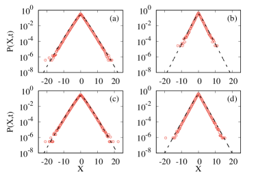
Figure 2: Comparison of numerically estimated $P(X,t)$ (red circles) against the solution given in (Universal to Non-Universal Transition of the statistics of Rare Events During the Spread of Random Walks) (black dashed line). The waiting time distributions are the following: (a) exponential mixture $\psi(\tau)=p_{1}r_{1}e^{-r_{1}\tau}+p_{2}r_{2}e^{-r_{2}\tau}$ with $r_{1}=1/4,r_{2}=5/2,p_{1}=1/4,p_{2}=3/4$ at $t=0.7$; (b) gamma distribution $\psi(\tau)=\tau^{3}e^{-\tau}/6$ at $t=0.8$; (c) half Gaussian distribution $\psi(\tau)=\sqrt{2/\pi}e^{-\tau^{2}/2}$ at $t=1.5$; (d) power law distribution $\psi(\tau)=1/(1+\tau)^{2}$ at $t=0.4$.

From Fig. 2 we see that the large deviation form of $P(X,t)$ evaluated in (Universal to Non-Universal Transition of the statistics of Rare Events During the Spread of Random Walks) agrees with numerically estimated $P(X,t)$ for different waiting time distributions. In other words, $P(X,t)$ possesses exponentially decaying tails in the limit of large $|X|/t$ when the distribution of jumps is Laplace distributed.

$P(X,t)$ derived in (Universal to Non-Universal Transition of the statistics of Rare Events During the Spread of Random Walks) holds for a wide class of waiting time distributions analytic near zero. This further implies that the rare fluctuations for a CTRW with Laplace distributed jumps are described by the large deviation principle Touchette (2009). In this regard, the case $\beta=1$ is analogous to the $\beta>1$ case discussed in Ref. Barkai and Burov (2020); Wang et al. (2020a); Pacheco-Pozo and Sokolov (2021) if we restrict our attention solely to the exponentially decaying fluctuations of $P(X,t)$. The analogy, however, ends here as for $\beta>1~{}N_{0}$ increases linearly with $|X|$ while for $\beta=1$, the growth is sublinear. Furthermore, for $\beta>1$ the PDF exhibits exponentially decaying tails with logarithmic corrections Barkai and Burov (2020) while for $\beta=1$ the corrections are of power-law type. Even though $P(X,t)$ exhibits exponentially decaying tails for both $\beta>1$ and $\beta=1$, different forms of correction term for the two cases “hints” towards a possible transition. Let us now explore the region $\beta<1$ to complete our understanding of this transition.

For $\beta<1$ the distribution of jumps belongs to the class of stretched exponential distributions Foss et al. (2013) which possesses heavy tails as $\int^{\infty}_{0}dx~{}e^{\lambda x}f(x)=\infty~{}\forall~{}\lambda>0$ and does not admit a large deviation form Touchette (2009). It is a well-known result that the family of stretched exponential distributions satisfies the big jump principleFoss et al. (2013); Vezzani et al. (2019); Wang et al. (2019); Vezzani et al. (2020); Burioni and Vezzani (2020)

$$P(x_{1}+\cdots+x_{N}\geq X)\stackrel{{\scriptstyle|X|\to\infty}}{{\sim}}P(\text{max}\{x_{1},...,x_{N}\}\geq X)$$ (12)

with the right hand side evaluating to $1-\Big{[}1-\int^{\infty}_{X}dx~{}f(x)\Big{]}^{N}$ for IID $x_{i}$. Hence, from (1) we have

$$\int^{\infty}_{X}dX~{}P(X,t)\stackrel{{\scriptstyle|X|\to\infty}}{{\sim}}1-G_{t}\Big{(}1-\int^{\infty}_{X}dx~{}f(x)\Big{)}$$ (13)

where $G_{t}(z)=\sum_{N=0}^{\infty}z^{N}Q_{t}(N)$. Furthermore, for large $|X|$ we have $\int^{\infty}_{X}dx~{}f(x)\sim 0$, as a result we can analyze $P(X,t)$ in terms of the behavior of $G_{t}(z)$ for $z$ in the neighborhood of unity. Now $G_{t}(1-\eta)\approx G_{t}(1)-\frac{\partial G}{\partial z}|_{z=1}\eta$ for $\eta$ small and $\frac{\partial G}{\partial z}=\sum_{N=1}^{\infty}NQ_{t}(N)z^{N-1}$. This implies $G_{t}\Big{(}1-\int^{\infty}_{X}dx~{}f(x)\Big{)}\approx 1-\langle N_{t}\rangle\int^{\infty}_{X}dx~{}f(x)$ and from here it follows that

$$P(X,t)\stackrel{{\scriptstyle|X|\to\infty}}{{\sim}}\langle N_{t}\rangle f(X).$$ (14)

The above equation implies that the probability of being at a location $X$ at time $t$ equals the mean number of jumps $\langle N_{t}\rangle$ up to time $t$ times the distribution of a single jump $f(X)$. With the distribution of a single jump known, we only need to estimate the mean number of jumps $\langle N_{t}\rangle$ which in the Laplace domain reads Klafter and Sokolov (2011) $\langle\tilde{N}_{s}\rangle=\frac{\tilde{\psi}_{s}}{s(1-\tilde{\psi}_{s})}$, where $\tilde{\psi}_{s}=\int^{\infty}_{0}dt~{}e^{-st}\psi(t)$ is the Laplace transform of $\psi(\tau)$. For $\psi(\tau)$ analytic near zero (cf. (7)) we have in the limit $t\to 0$ sup

$$\langle N_{t}\rangle\approx\frac{C_{A}\Gamma(A+1)}{\Gamma(A+2)}t^{A+1}+\frac{C_{A+1}\Gamma(A+2)}{\Gamma(A+3)}t^{A+2}.$$ (15)

The reason to focus on the $t\to 0$ limit is that it allows us to address the rare fluctuations exhibited by the CTRW at finite times, that is, $|X|/t\to\infty$. Specifically, in many experiments that show Laplace decay of the PDF, the non-Gaussian behavior was spotted for short enough times Chechkin et al. (2017). For a long measurement time, the Gaussian center eventually takes over Vitali et al. (2022). Notwithstanding the limited range of validity of (15), $P(X,t)$ derived in (14) holds at arbitrary times,

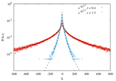
Figure 3: Numerically estimated $P(X,t)$ for a CTRW with jumps following a generalized Gaussian distribution with PDF $f(x)=\frac{\beta}{2\Gamma(1/\beta)}e^{-|x|^{\beta}}$ with $\beta=1/3$, for $\psi(\tau)=\sqrt{2/\pi}e^{-\tau^{2}/2}$ (red circles) and $\beta=1/2$ for $\psi(\tau)=\frac{1}{(1+\tau)^{2}}$ (blue squares). The black dashed lines represent the analytical form from (14).

and is in excellent agreement with numerical simulations (see Fig. 3). It is important to notice that the average number of jumps, $\langle N_{t}\rangle$, was previously found to be an important quantity determining the tails of the PDF for Lévy walks Vezzani et al. (2019, 2020); Wang et al. (2020b).

The result in (14) shows that the parameter range $\beta\in(0,1)$ is markedly different from the region $\beta\geq 1$. In addition, differences in the nature of the PDF of CTRW at $\beta=1$ and $\beta>1$ imply towards the fact that the PDF of a CTRW critically changes at $\beta=1$, which is essentially the same value for which the order parameter $F_{\beta}(X)$ shows a critical transition. The evaluation of $P(X,t)$ further corroborates our assertion of a universal to non-universal transition as seen from the analysis of $F_{\beta}(X)$ (see Fig. 1). The fact that $\lim_{|X|\to\infty}F_{\beta}(X)=0$ for $\beta\geq 1$ is analogous to saying that $P(X,t)\sim\exp[-tI(|X|/t)]$ exists with a nontrivial rate function $I(|X|/t)$ for every $\beta\geq 1$. This rate function $I(z)$ attains a linear growth for large $z$ and, therefore, the universal exponential decay of the PDF, i.e., $P(X,t)\sim e^{-|X|}$. On the other hand, for $\beta<1$ we had seen from Fig. 1 that $\lim_{|X|\to\infty}F_{\beta}(X)=c_{\beta}>0$. Eq. (14) shows that for $\beta<1$, the rate function $I(|X|/t)$ is trivially zero. For large $|X|$, the decay of the PDF is stretched exponential, i.e., $P(X,t)\sim e^{-|X|^{\beta}}$, that specifically depends on the parameter $\beta$. Notice that the transition of $\phi_{\alpha}(t)$ in the long time limit represents the transition from diffusion to subdiffusion and is accompanied by the transition of the PDF (in the $|X|/t\to 0$ limit) from the universal Gaussian form to the $\alpha$-stable Lévy type that explicitly depends on $\alpha$.

Hopping dynamics which is an intrinsic feature of CTRW, has been ubiquitously observed in polymer melts Schweizer and Saltzman (2004), colloidal suspensions Schweizer and Saltzman (2003), rodlike particles through smectic layers Lettinga and Grelet (2007); Grelet et al. (2008), polymer glasses Warren and Rottler (2010), binary mixtures Miotto et al. (2021), in one, two, and three spatial dimensions Aoki et al. (2013), to mention a few. A characteristic feature of motion in glassy materials Chaudhuri et al. (2007, 2008); Wang et al. (2009, 2012) and at the liquid-solid interface Skaug et al. (2013); Wang et al. (2017), where hopping dynamics is observed, has been the exponential decay of the tails of the positional PDF. Exponential decay, however, is the rule whenever hopping dynamics is in play Barkai and Burov (2020), making it a universal feature of transport in heterogeneous media. But in some situations, like the case of particles with a constant supply of energy (e.g., run and tumble particles), the particles can perform really long jumps during their exploration of the heterogeneous media Mori et al. (2021). Our work shows that a critical transition is expected for any system involving such hops. This critical transition manifests itself at the level of the positional PDF, where the universality of Laplace tails ceases to exist. While the universal tails are an outcome of an accumulation of many events and the applicability of the large-deviation principle, the specific tails for $\beta<1$ are determined by one single event, that is, the big-jump principle.

Unlike a diffusion-to-subdiffusion transition which takes place at long times and is accompanied by divergences of the mean trapping time, the phase transition reported in the present study is free from such divergences. The mean length of a hop can be finite, and the transition is observed at finite times. Furthermore, while the temporal properties of rare events leading to subdiffusion affect the bulk, rare spatial events manifest themselves mainly in the tails of the PDF. Interestingly, the temporal features do not affect the spatial dependence of the statistics of the rare events, that is, the tails of $P(X,t)$.

Acknowledgments: This work was supported by the Israel Science Foundation Grant No. 2796/20. RKS thanks the Israel Academy of Sciences and Humanities (IASH) and the Council of Higher Education (CHE) Fellowship.

References

- Amihud et al. (1990) Y. Amihud, H. Mendelson, and R. Wood, J. Portfolio Management 16, 65 (1990).
- Lomnitz (1966) C. Lomnitz, Rev. Geophys. 4, 377 (1966).
- Leckebusch and Ulbrich (2004) G. C. Leckebusch and U. Ulbrich, Global and Planetary Change 44, 181 (2004).
- Metzler and Klafter (2000) R. Metzler and J. Klafter, Phys. Rep. 339, 1 (2000).
- Weiss and Rubin (1983) G. H. Weiss and R. J. Rubin, Adv. Chem. Phys. 52, 363 (1983).
- Alexander et al. (1981) S. Alexander, J. Bernasconi, W. Schneider, and R. Orbach, Rev. Mod. Phys. 53, 175 (1981).
- Havlin and Ben-Avraham (1987) S. Havlin and D. Ben-Avraham, Adv. Phys. 36, 695 (1987).
- Isichenko (1992) M. B. Isichenko, Rev. Mod. Phys. 64, 961 (1992).
- Shlesinger et al. (1993) M. F. Shlesinger, G. M. Zaslavsky, and J. Klafter, Nature 363, 31 (1993).
- Haus and Kehr (1987) J. W. Haus and K. W. Kehr, Phys. Rep. 150, 263 (1987).
- Scher et al. (1991) H. Scher, M. F. Shlesinger, and J. T. Bendler, Physics Today 44, 26 (1991).
- Binder and Young (1986) K. Binder and A. P. Young, Rev. Mod. Phys. 58, 801 (1986).
- Manzo et al. (2015) C. Manzo, J. A. Torreno-Pina, P. Massignan, G. J. Lapeyre Jr, M. Lewenstein, and M. F. G. Parajo, Phys. Rev. X 5, 011021 (2015).
- Granéli et al. (2006) A. Granéli, C. C. Yeykal, R. B. Robertson, and E. C. Greene, Proc. Natl. Acad. Sci. U.S.A. 103, 1221 (2006).
- Wang et al. (2006) Y. Wang, R. H. Austin, and E. C. Cox, Phys. Rev. Lett. 97, 048302 (2006).
- Jeon et al. (2011) J.-H. Jeon, V. Tejedor, S. Burov, E. Barkai, C. Selhuber-Unkel, K. Berg-Sørensen, L. Oddershede, and R. Metzler, Phys. Rev. Lett. 106, 048103 (2011).
- Bouchaud (1992) J.-P. Bouchaud, J. Phys. I France 2, 1705 (1992).
- Akimoto et al. (2016) T. Akimoto, E. Barkai, and K. Saito, Phys. Rev. Lett. 117, 180602 (2016).
- Barkai and Cheng (2003) E. Barkai and Y.-C. Cheng, J. Chem. Phys. 118, 6167 (2003).
- Rebenshtok and Barkai (2007) A. Rebenshtok and E. Barkai, Phys. Rev. Lett. 99, 210601 (2007).
- Bel and Barkai (2005) G. Bel and E. Barkai, Phys. Rev. Lett. 94, 240602 (2005).
- Burov and Barkai (2007) S. Burov and E. Barkai, Phys. Rev. Lett. 98, 250601 (2007).
- Pronin (2022) K. Pronin, Physica A: Statistical Mechanics and its Applications 596, 127180 (2022).
- Sabhapandit (2011) S. Sabhapandit, Europhys. Lett. 94, 20003 (2011).
- Burov (2017) S. Burov, Phys. Rev. E 96, 050103 (2017).
- Shafir and Burov (2022) D. Shafir and S. Burov, J. Stat. Mech.: Theor. Exp. 2022, 033301 (2022).
- Klafter and Sokolov (2011) J. Klafter and I. M. Sokolov, First steps in random walks: from tools to applications (OUP Oxford, 2011).
- Bouchaud and Georges (1990) J.-P. Bouchaud and A. Georges, Phys. Rep. 195, 127 (1990).
- Uchaikin (2003) V. V. Uchaikin, Physics-Uspekhi 46, 821 (2003).
- Garoni and Frankel (2002) T. M. Garoni and N. E. Frankel, J. Math. Phys. 43, 2670 (2002).
- Chechkin et al. (2017) A. V. Chechkin, F. Seno, R. Metzler, and I. M. Sokolov, Phys. Rev. X 7, 021002 (2017).
- Pastore et al. (2021) R. Pastore, A. Ciarlo, G. Pesce, F. Greco, and A. Sasso, Phys. Rev. Lett. 126, 158003 (2021).
- Uttieri et al. (2021) M. Uttieri, P. Hinow, R. Pastore, G. Bianco, M. R. d’Alcalá, and M. G. Mazzocchi, J. R. Soc. Interface 18, 20210270 (2021).
- Rusciano et al. (2022) F. Rusciano, R. Pastore, and F. Greco, Phys. Rev. Lett. 128, 168001 (2022).
- Xue et al. (2016) C. Xue, X. Zheng, K. Chen, Y. Tian, and G. Hu, J. Phys. Chem. Lett. 7, 514 (2016).
- Wang et al. (2017) D. Wang, H. Wu, and D. K. Schwartz, Phys. Rev. Lett. 119, 268001 (2017).
- Chaudhuri et al. (2007) P. Chaudhuri, L. Berthier, and W. Kob, Phys. Rev. Lett. 99, 060604 (2007).
- Chaudhuri et al. (2008) P. Chaudhuri, Y. Gao, L. Berthier, M. Kilfoil, and W. Kob, J. Phys.: Condens. Matter 20, 244126 (2008).
- Wang et al. (2012) B. Wang, J. Kuo, S. C. Bae, and S. Granick, Nature Materials 11, 481 (2012).
- Barkai and Burov (2020) E. Barkai and S. Burov, Phys. Rev. Lett. 124, 060603 (2020).
- Wang et al. (2020a) W. Wang, E. Barkai, and S. Burov, Entropy 22, 697 (2020a).
- Pacheco-Pozo and Sokolov (2021) A. Pacheco-Pozo and I. M. Sokolov, Phys. Rev. E 103, 042116 (2021).
- Foss et al. (2013) S. Foss, D. Korshunov, and S. Zachary, in An Introduction to Heavy-Tailed and Subexponential Distributions (Springer, 2013), pp. 7–42.
- Embrechts et al. (2013) P. Embrechts, C. Klüppelberg, and T. Mikosch, Modelling extremal events: for insurance and finance, vol. 33 (Springer Science & Business Media, 2013).
- Kutner (2002) R. Kutner, Chem. Phys. 284, 481 (2002).
- De Mulatier et al. (2013) C. De Mulatier, A. Rosso, and G. Schehr, J. Stat. Mech.: Theory and Experiment 2013, P10006 (2013).
- Majumdar et al. (2005) S. N. Majumdar, M. Evans, and R. Zia, Phys. Rev. Lett. 94, 180601 (2005).
- Hollander (2000) F. Hollander, Large deviations, vol. 14 (American Mathematical Soc., 2000).
- Ellis (1999) R. S. Ellis, Physica D: Nonlinear Phenomena 133, 106 (1999).
- Dembo and Zeitouni (2009) A. Dembo and O. Zeitouni, Large deviations techniques and applications, vol. 38 (Springer Science & Business Media, 2009).
- Nickelsen and Touchette (2018) D. Nickelsen and H. Touchette, Phys. Rev. Lett. 121, 090602 (2018).
- Touchette (2009) H. Touchette, Phys. Rep. 478, 1 (2009).
- He et al. (2008) Y. He, S. Burov, R. Metzler, and E. Barkai, Phys. Rev. Lett. 101, 058101 (2008).
- Magdziarz et al. (2008) M. Magdziarz, A. Weron, and J. Klafter, Phys. Rev. Lett. 101, 210601 (2008).
- Derrida (1997) B. Derrida, Physica D: Nonlinear Phenomena 107, 186 (1997).
- Majumdar (2010) S. N. Majumdar, Physica A 389, 4299 (2010).
- Mounaix et al. (2018) P. Mounaix, S. N. Majumdar, and G. Schehr, J. Stat. Mech. 2018, 083201 (2018).
- Mori et al. (2020) F. Mori, S. N. Majumdar, and G. Schehr, Phys. Rev. E 101, 052111 (2020).
- Höll and Barkai (2021) M. Höll and E. Barkai, Eur. Phys. J. B 94, 1 (2021).
- Nardon and Pianca (2009) M. Nardon and P. Pianca, J. Stat. Comp. Sim. 79, 1317 (2009).
- Nyawo and Touchette (2017) P. T. Nyawo and H. Touchette, Europhys. Lett. 116, 50009 (2017).
- Nyawo and Touchette (2018) P. T. Nyawo and H. Touchette, Phys. Rev. E 98, 052103 (2018).
- Garrahan et al. (2007) J. P. Garrahan, R. L. Jack, V. Lecomte, E. Pitard, K. van Duijvendijk, and F. van Wijland, Phys. Rev. Lett. 98, 195702 (2007).
- Jack and Sollich (2013) R. L. Jack and P. Sollich, J. Phys. A: Math. Theor. 47, 015003 (2013).
- Watson (1922) G. N. Watson, A treatise on the theory of Bessel functions, vol. 3 (The University Press, 1922).
- Gradshteyn and Ryzhik (2014) I. S. Gradshteyn and I. M. Ryzhik, Table of integrals, series, and products (Academic press, 2014).
- Burov (2020) S. Burov, arXiv:2007.00381 (2020).
- Daniels (1954) H. E. Daniels, Ann. Math. Stat. p. 631 (1954).
- Vezzani et al. (2019) A. Vezzani, E. Barkai, and R. Burioni, Phys. Rev. E 100, 012108 (2019).
- Wang et al. (2019) W. Wang, A. Vezzani, R. Burioni, and E. Barkai, Phys. Rev. Res. 1, 033172 (2019).
- Vezzani et al. (2020) A. Vezzani, E. Barkai, and R. Burioni, Sci. Rep. 10, 2732 (2020).
- Burioni and Vezzani (2020) R. Burioni and A. Vezzani, J. Stat. Mech.: Theor. Exp. p. 034005 (2020).
- (73) See Supplemantary Material.
- Vitali et al. (2022) S. Vitali, P. Paradisi, and G. Pagnini, J. Phys. A: Math. Theor. 55, 224012 (2022).
- Wang et al. (2020b) W. Wang, M. Höll, and E. Barkai, Phys. Rev. E 102, 052115 (2020b).
- Schweizer and Saltzman (2004) K. S. Schweizer and E. J. Saltzman, J. Chem. Phys. 121, 1984 (2004).
- Schweizer and Saltzman (2003) K. S. Schweizer and E. J. Saltzman, J. Chem. Phys. 119, 1181 (2003).
- Lettinga and Grelet (2007) M. P. Lettinga and E. Grelet, Phys. Rev. Lett. 99, 197802 (2007).
- Grelet et al. (2008) E. Grelet, M. P. Lettinga, M. Bier, R. Van Roij, and P. Van der Schoot, J. Phys.: Condens. Matter 20, 494213 (2008).
- Warren and Rottler (2010) M. Warren and J. Rottler, The Journal of chemical physics 133, 164513 (2010).
- Miotto et al. (2021) J. M. Miotto, S. Pigolotti, A. V. Chechkin, and S. Roldán-Vargas, Phys. Rev. X 11, 031002 (2021).
- Aoki et al. (2013) K. M. Aoki, S. Fujiwara, K. Sogo, S. Ohnishi, and T. Yamamoto, Crystals 3, 315 (2013).
- Wang et al. (2009) B. Wang, S. M. Anthony, S. C. Bae, and S. Granick, Proc. Natl. Acad. Sci. U.S.A. 106, 15160 (2009).
- Skaug et al. (2013) M. J. Skaug, J. Mabry, and D. K. Schwartz, Phys. Rev. Lett. 110, 256101 (2013).
- Mori et al. (2021) F. Mori, G. Gradenigo, and S. N. Majumdar, J. Stat. Mech.: Theor. Exp. 2021, 103208 (2021).