Iterative two-level algorithm for nonsymmetric or indefinite elliptic problems

Abstract

In this paper, a new iterative two-level algorithm is presented for solving the finite element discretization for nonsymmetric or indefinite elliptic problems. The iterative two-level algorithm uses the same coarse space as the traditional two-grid algorithm, but its “fine space” uses the higher oder finite element space under the coarse grid. Therefore, the iterative two-level algorithm only needs one grid, and the computational cost is much lower than the traditional iterative two-grid algorithm. Finally, compared with the traditional two-grid algorithm, numerical experiments show that the computational cost is lower to achieve the same convergence order.

1 Introduction

We consider the following Dirichlet boundary value problems for general second-order elliptic partial differential equations

$$-\mathrm{div}(\boldsymbol{\alpha}(x)\nabla u)+\boldsymbol{\beta}(x)\cdot\nabla u+\gamma(x)u=f \mbox{in $\Omega$ },$$ (1.1)

$$u=0 \mbox{on $\partial\Omega$ },$$ (1.2)

where the coefficient $\boldsymbol{\alpha}(x)\in\mathbb{R}^{d}\times\mathbb{R}^{d}$ is smooth functions on $\bar{\Omega}$, and satisfies consistent ellipticity, namely, there are minimum and maximum eigenvalues $\alpha_{*}$ and $\alpha^{*}$ respectively, satisfying $\alpha_{*}|\xi|^{2}\leqslant\mathbf{\alpha}(x)\xi\cdot\xi\leqslant\alpha^{*}|\xi|^{2},~{}~{}\forall\xi\in\mathbb{R}^{d}$. Both $\boldsymbol{\beta}(x)\in\mathbb{R}^{d}$ and $\gamma(x)\in\mathbb{R}^{1}$ are smooth functions on $\bar{\Omega}$, and $f\in L^{2}(\Omega)$ is a given function. Noting that when $\boldsymbol{\beta}(x)\neq\boldsymbol{0}$, the continuous variational problems (CVP) of (1.1)-(1.2) are nonsymmetric, and when $\gamma(x)<0$, the CVP of (1.1)-(1.2) may be indefinite.

The two-grid (TG) algorithm was first introduced by Xu [6] for solving nonasymmetric or indefinite problems. The main idea of the TG algorithm is to solve the original problems on the coarse mesh to obtain an approximate finite element solution, and then use the approximate solution to solve the corresponding linear symmetric positive definite problems on the fine mesh. Over the last two decades, the TG algorithm has been widely used to solve many problems, such as nonlinear elliptic problems [1, 10], semilinear parabolic equations [5], nonlinear parabolic equations [3, 2], Poisson-Nernst-Planck problems [7], and Maxwell equations [8, 9].

The main objective of this paper is to propose a new iterative two-level algorithm. Compared with the traditional iterative two-grid algorithm, our algorithm needs only one mesh and takes less CPU time to achieve the same accuracy.

In this work, we first present elliptic problems discretized by the finite element method. Then, we propose an iterative two-level algorithm. Finally, some numerical results are presented to illustrate the efficiency of the proposed algorithms.

2 Finite element discretizations

Given $S\subset\mathbb{R}^{d}(d=2,3)$, we denote $W^{1,2}(S)$ as the standard Sobolev space with norm $\|\cdot\|_{1,2,S}$. For simplicity of notation, we denote $\|\cdot\|_{1}=\|\cdot\|_{1,2,\Omega}$, and $H^{1}_{0}(\Omega):=\{u\in H^{1}(\Omega):u|_{\partial\Omega}=0\}$ in the sense of trace. We define the following two bilinear forms

$$a(u,v) := \int_{\Omega}(\boldsymbol{\alpha}(x)\nabla u)\cdot\nabla v\mathrm{d}x,$$ (2.1)

$$\hat{a}(u,v) := a(u,v)+\int_{\Omega}(\boldsymbol{\beta}(x)\cdot\nabla u+\gamma(x)u)v\mathrm{d}x.$$ (2.2)

Then, we obtain the CVP of (1.1)-(1.2): Find $u\in H_{0}^{1}(\Omega)$, such that

$$\hat{a}(u,v)=(f,v),~{}~{}\forall v\in H_{0}^{1}(\Omega).$$ (2.3)

We assume that $\Omega$ is partitioned by a quasi-uniform division $\mathcal{T}_{h}=\{\tau_{i}\}$. By this we mean that $\tau_{i}$’s are simplexes of the size $h$ with $h\in(0,1)$ and $\bar{\Omega}=\cup_{i}\tau_{i}$. For the given quasi-uniform division $\mathcal{T}_{h}$, the conforming finite element space is defined as follows

$$V_{h}^{l}:=\{v\in C(\Omega):v|_{\tau}\in\mathbb{P}_{l}(\tau),~{}\forall\tau\in\mathcal{T}_{h},~{}v|_{\partial\Omega}=0\},$$

where $\mathbb{P}_{l}(\tau)$ is the space of polynomial of degree not greater than a positive integer $l$ on the subdivision element $\tau$. The discrete variational problems of (2.3) is to find $u_{h}^{l}\in V_{h}^{l}$, such that

$$\hat{a}(u_{h}^{l},v_{h}^{l})=(f,v_{h}^{l}),~{}~{}\forall v_{h}^{l}\in V_{h}^{l}.$$ (2.4)

3 Iterative two-level algorithm

The basic mechanism of the classical iterative two-grid algorithm is two quasi-uniform tetrahedral nested meshes of $\Omega$, namely the fine space $V_{h}^{k,l}$ and the coarse space $V_{H}^{k,l}$, with two different meshes sizes $h$ and $H(h<H)$. Furthermore, in the application given in the succeeding text, we shall always assume that $H=O\left(h^{\lambda}\right)\text{ for some }0<\lambda<1.$

Algorithm 3.1 (Algorithm 4.1 of [6]).

Let $u_{h}^{l,0}=0$; assume that $u_{h}^{l,k}\in{V}_{h}^{l}(k\geq 0)$ has been obtained, $u_{h}^{l,k+1}\in{V}_{h}^{l}$ is defined as follows:

1.

Find $e_{H}^{l,k}\in V_{H}^{l}$, such that $\hat{a}(e_{H}^{l,k},v_{H}^{l})=(f,v_{H}^{l})-\hat{a}(u^{l,k}_{h},v_{H}^{l}),\ \forall v_{H}^{l}\in V_{H}^{l}.$

2.

Find $u_{h}^{l,k+1}\in V_{h}^{l}$, such that $a(u_{h}^{l,k+1},v_{h}^{l})=(f,v_{h}^{l})-N(u_{h}^{l,k}+e_{H}^{l,k},v_{h}^{l}),\ \forall v^{l}_{h}\in V_{h}^{l},$

where $N(u,v):=\hat{a}(u,v)-a(u,v),\quad\forall u,v\in H_{0}^{1}(\Omega).$

Assume that $u_{h}^{l,k+1}\in V_{h}^{l}$ is the solution obtained by Algorithm 3.1 with $k\geq 1$, then we have (see Theorem 4.4 of [6])

$$\|u-u_{h}^{l,k+1}\|_{1}\lesssim(h^{l}+H^{k+l})\|u\|_{l+1},$$ (3.1)

which means that the two-grid solution given by Algorithm 3.1 can effectively approximate the finite element solution $u_{h}^{l}$ of (2.4).

Remark 3.1.

In order to obtain the optimal convergence order in (3.1), we should assume that $H$ and $h$ satisfy the relation $h=O(H^{\frac{l+k}{l}})$. However, there are exact nested grids, which satisfy $h=O(H^{\frac{l+k}{l}})$, very difficult to implement.

Next, we consider replacing $V^{l}_{h}$ with $V_{H}^{s}(s\geq l+1)$ in the second step of Algorithm 3.1, and obtain the following algorithm.

Algorithm 3.2.

Let $\hat{u}_{H}^{l,0}=0$; assume that $\hat{u}_{H}^{s,k}\in{V}_{H}^{s}(k\geq 0)$ has been obtained, $\hat{u}_{H}^{s,k+1}\in{V}_{H}^{s}$ is defined as follows:

1.

Find $e_{H}^{l,k}\in V_{H}^{l}$, such that $\hat{a}(e_{H}^{l,k},v_{H}^{l})=(f,v_{H}^{l})-\hat{a}(\hat{u}^{s,k}_{H},v_{H}^{l}),\ \forall v_{H}^{l}\in V_{H}^{l}.$

2.

Find $\hat{u}_{H}^{s,k+1}\in V_{H}^{s}$, such that $a(\hat{u}_{H}^{s,k+1},v_{H}^{s})=(f,v_{H}^{s})-N(\hat{u}_{H}^{s,k}+e_{H}^{l,k},v_{H}^{s}),\ \forall v^{s}_{H}\in V_{H}^{s}.$

Remark 3.2.

Comparing Algorithm 3.1 with Algorithm 3.2, although the SPD problems are solved in the second step of the algorithm, $V_{H}^{s}$ has fewer degrees of freedom than $V_{h}^{l}$ (See Table 1), which can greatly reduce the computation time.

$\mathcal{T}_{H}$	$dof(V_{H}^{3})$	$dof(V_{h}^{3})$	$dof(V_{H}^{4})$	$dof(V_{H}^{5})$	$dof(V_{H}^{6})$
1/9	784	59536	1369	2116	3025
1/10	961	90601	1681	2601	3721
1/11	1156	132496	2025	3136	4489
1/12	1369	187489	2401	3721	5329

Table 1: Taking $h=H^{2}$, $V_{H}^{4}$, $V_{H}^{5}$, $V_{H}^{6}$ and $V_{h}^{3}$ degrees of freedom comparison

4 Numerical results

In this section, numerical experiments are carried out to verify the effectiveness of the iterative two-level algorithm. We performed all experiments for our iterative two-level algorithm with the help of the software package Fenics [4].

Example 4.1.

We consider model problems (1.1)-(1.2), where the computational domain is $\Omega=(0,1)^{2}$, the coefficients are $\alpha=1.0$, $\boldsymbol{\beta}=(0,0)^{t}$ and $\gamma=-10$, the exact solution is $u=\sin(\pi x)\sin(\pi y)$, and $f$ can be obtained by substituting the exact solution into equation (1.1).

We first partition the $x-$ axis and $y-$ axis of the domain $\Omega$ into equally distributed $M$ subintervals, then divide each square into two triangles by using the line with slope $-1$. Hence, we obtain a sequence of nested and structured grids and the corresponding meshes as $\mathcal{T}_{H}$ with $H=1/M$, where $M\geq 2$ is an integer, see Figure 1. We choose the piecewise conform $l$ order finite element spaces $V_{H}^{l}$ based on the meshes $\mathcal{T}_{H}$. For Algorithm 3.1, we choose $h=H^{2}$.

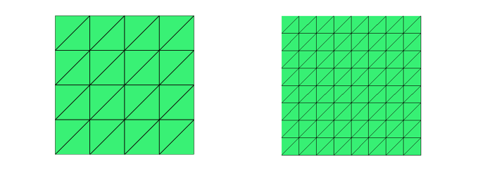
Figure 1: Structured grids with $\mathcal{T}_{1/4}$ (left) and $\mathcal{T}_{1/8}$ (right).

	Algorithm 3.1, $l=3$, $k=3$			Algorithm 3.2, $l=3$, $s=6$, $k=3$
$H$	$\|u-u_{h}^{3,3}\|_{1}$	$\|u-u_{h}^{3,3}\|_{1}*H^{-6}$	CPU	$\|u-\hat{u}_{H}^{6,3}\|_{1}$	$\|u-\hat{u}_{H}^{6,3}\|_{1}*H^{-6}$	CPU
1/9	9.8925E-07	5.2573E-01	6.1544	5.7750E-08	3.0691E-02	0.2503
1/10	5.2609E-07	5.2609E-01	9.0338	3.0706E-08	3.0706E-02	0.3082
1/11	2.9711E-07	5.2635E-01	16.177	1.7339E-08	3.0717E-02	0.3644
1/12	1.7634E-07	5.2655E-01	24.047	1.0290E-08	3.0726E-02	0.4347

Table 2: Compare the $H^{1}$ error estimate between the classical iterative two-grid algorithm 3.1 and the iterative two-level algorithm 3.2.

From Table 2, we can observe that both our algorithm and the traditional iterative mesh can reach the optimal convergence order. And to achieve the same accuracy, our algorithm uses less CPU time.

	Algorithm 3.2, $l=3$, $s=4$, $k=3$			Algorithm 3.2, $l=3$, $s=5$, $k=3$
$H$	$\|u-\hat{u}_{H}^{4,3}\|_{1}$	$\|u-\hat{u}_{H}^{4,3}\|_{1}*H^{-4}$	CPU	$\|u-\hat{u}_{H}^{5,3}\|_{1}$	$\|u-\hat{u}_{H}^{5,3}\|_{1}*H^{-5}$	CPU
1/9	3.6409E-05	2.3888E-01	0.1383	1.6093E-06	9.5028E-02	0.1825
1/10	2.3903E-05	2.3903E-01	0.1633	9.5141E-07	9.5141E-02	0.2172
1/11	1.6334E-05	2.3915E-01	0.2785	5.9129E-07	9.5228E-02	0.2571
1/12	1.1538E-05	2.3924E-01	0.2237	3.8298E-07	9.5299E-02	0.3020

Table 3: the $H^{1}$ error estimate of the iterative two-level algorithm 3.2.

From the Tables 2- 3, it can be found that when the degree of the coarse space polynomial degree $l=3$ is fixed, as the degree of the fine space polynomial increases once, the convergence order of the error estimates in $H^{1}$-norm for the solution of the algorithm 3.2 increase by one order. It can be seen that the errors in $H^{1}$-norm for the solution of the algorithm 3.2 depend on the value of $s$.

Example 4.2.

We consider model problems (1.1)-(1.2), where the computational domain is $\Omega=(0,1)^{2}$, the coefficients are $\alpha=1.0$, $\boldsymbol{\beta}=(0,0)^{t}$ and $\gamma=-10$, the exact solution is $u=x(1-x)^{2}y(1-y)^{2}$, and $f$ can be obtained by substituting the exact solution into equation (1.1).

	Algorithm 3.1, $l=3$, $k=3$			Algorithm 3.2, $l=3$, $s=6$, $k=3$
$H$	$\|u-u_{h}^{3,3}\|_{1}$	$\|u-u_{h}^{3,3}\|_{1}*H^{-6}$	CPU	$\|u-\hat{u}_{H}^{6,3}\|_{1}$	$\|u-\hat{u}_{H}^{6,3}\|_{1}*H^{-6}$	CPU
1/9	6.0567E-08	3.2188E-02	6.0850	2.8919E-13	1.5369E-07	0.1901
1/10	3.2255E-08	3.2255E-02	8.9463	1.2153E-13	1.2153E-07	0.2335
1/11	1.8235E-08	3.2305E-02	16.0683	7.9992E-14	1.4171E-07	0.2751
1/12	1.0832E-08	3.2344E-02	23.8708	7.8801E-14	2.3530E-07	0.3291

Table 4: Compare the $H^{1}$ error estimate between the classical iterative two-grid algorithm 3.1 and the iterative two-level algorithm 3.2.

	Algorithm 3.2, $l=3$, $s=4$, $k=3$			Algorithm 3.2, $l=3$, $s=5$, $k=3$
$H$	$\|u-\hat{u}_{H}^{4,3}\|_{1}$	$\|u-\hat{u}_{H}^{4,3}\|_{1}*H^{-4}$	CPU	$\|u-\hat{u}_{H}^{5,3}\|_{1}$	$\|u-\hat{u}_{H}^{5,3}\|_{1}*H^{-5}$	CPU
1/9	1.9981E-06	1.3110E-02	0.1035	5.2140E-08	3.0788E-03	0.1380
1/10	1.3129E-06	1.3129E-02	0.1214	3.0796E-08	3.0796E-03	0.1637
1/11	8.9783E-07	1.3145E-02	0.1420	1.9126E-08	3.0803E-03	0.1938
1/12	6.3456E-07	1.3158E-02	0.1661	1.2381E-08	3.0809E-03	0.2273

Table 5: the $H^{1}$ error estimate of the iterative two-level algorithm 3.2.

The same conclusions can be observed in Tables 4 and 5 as in Tables 2 and 3.

References

References

- [1] C.J. Bi, C. Wang, Y.P. Lin, A posteriori error estimates of two-grid finite element methods for nonlinear elliptic problems, J. Sci. Comput. 74 (1) (2018) 23–48.
- [2] C. Dawson, M. Wheeler, C. Woodward, A two-grid finite difference scheme for nonlinear parabolic equations, SIAM J Numer. Anal. 35 (2) (1998) 435–452.
- [3] C.N. Dawson, M. F. Wheeler, Two-grid methods for mixed finite element approximations of nonlinear parabolic equations, Contemp. Math., 180 (1994) 191–203.
- [4] A. Logg, K.A. Mardal, G. Wells, Automated solution of differential equations by the finite element method, Springer, 2012.
- [5] M. Marion, J.C. Xu, Error estimates on a new nonlinear Galerkin method based on two-grid finite elements, SIAM J. Numer. Anal. 32 (4) (1995) 1170–1184.
- [6] J.C. Xu, Two-grid discretization techniques for linear and nonlinear PDEs, SIAM J. Numer. Anal. 33 (5) (1996) 1759–1777.
- [7] Y. Yang, B.Z. Lu, Y. Xie, A decoupling two-grid method for the steady-state poisson-nernst-planck equations, J. Comput. Math. 37 (4) (2019) 556–578.
- [8] L.Q. Zhong, C.M. Liu, S. Shu, Two-level additive preconditioners for edge element discretizations of time-harmonic Maxwell equations, Comput. Math. Appl. 66 (4) (2013) 432–440.
- [9] L.Q. Zhong, S. Shu, J.X. Wang, J.C. Xu, Two-grid methods for time-harmonic Maxwell equations, Numer. Linear Algebra Appl. 20 (1) (2013) 93–111.
- [10] L.Q. Zhong, L.L. Zhou, C.M. Liu, J. Peng, Two-grid IPDG discretization scheme for nonlinear elliptic PDEs, Commun. Nonlinear Sci. Numer. Simul. 95 (2021) 105587.