Operator theory, kernels, and feedforward neural networks

Abstract.

In this paper we show how specific families of positive definite kernels serve as powerful tools in analyses of iteration algorithms for multiple layer feedforward Neural Network models. Our focus is on particular kernels that adapt well to learning algorithms for data-sets/features which display intrinsic self-similarities at feedforward iterations of scaling.

1. Introduction

Recently many authors have offered diverse approaches to feedforward Neural Network (NN) algorithms [ZC23, AK23, HL23, DWZ⁺23], as well as optimization terms based on kernels. Here we establish some new results in operator theory, and we bring them to bear on the problem. The list of applications of feedforward NN models includes a variety of machine learning settings, and deep NN based on kernels [GK23, MK23, BSW23, SHO22, GKNV22, GPR⁺21, Kut20, GKP20].

A common theme in feedforward NN models is specific prescribed iterations which entail (i) ReLu functions [JR23, OSZ22, CKM22, CCK22, JR22, CL22], (ii) substitution from prescribes systems of affine mappings. Moreover, (iii) each step is then linked to the next with a choice of an activation function. In this paper we show that there are natural positive definite kernels associated with the three steps going into feedforward NN constructions, as well as to their iteration. We believe that this then yields a more direct tool for kernel-based feedforward NN models. This advantage of our approach is based on two facts. First, we identify a direct notion of kernel iteration which accounts for traditional function theoretic feedforward NN steps. Secondly, our approach offers a more direct and natural choices of kernels which govern approximations involved in deep NN models, for example graph NN constructions.

While positive definite kernels and their associated reproducing kernel Hilbert spaces have found diverse applications in pure and applied mathematics, we shall focus here on a new role of kernels in feedforward network models. In more detail, the main purpose of our paper is a presentation of choices of particular families of positive definite kernels which serve as powerful tools in analyses of multiple layer feedforward Neural Networks.

In general, reproducing kernel constructions, and the corresponding RKHSs are powerful tools in diverse applications. In the present framework of kernel neural networks (KNNs) , their role may be summarized as follows: Starting with the problem at hand, when we build our RKHS$(\mu)$ via IFS iterations (e.g., via Cantor-like fractal limits), then the Cantor-like $\mu$ activation functions arise as relative reproducing dipole functions for RKHS$(\mu)$ as in 3.1 below.

2. Neural networks (NN), and reproducing kernel Hilbert spaces (RKHS)

A main theme in our paper is a development of new tools for design of feedforward Neural Network constructs. For this purpose we point out the use of positive definite kernels, and associated generating function for the NN algorithms. These kernel based functions include the more familiar ReLu functions, see Theorems 3.3 and 3.4 below. We stress that the particular RKHS constructs will be relative in the sense of Theorems 3.3 and 3.4, i.e., the inner product reproduces differences of function values.

Our approach to the use of kernels and functions for feedforward Neural Network (NN) algorithms, is based on a systematic study of two classes of operators. They act as follows: (i) between prescribed kernel Hilbert spaces, and (ii) other operators acting at indexed levels in the network, i.e., operators acting at fixed levels, so within choices of kernel Hilbert spaces. Case (i) includes a systematic study of composition operators (see Corollaries 2.7 and 2.9) in the context of kernel Hilbert spaces; and case (ii), the study of multiplier operators and their adjoints, see e.g., 2.15. We emphasize that the two classes of operations discussed below depend on choices of kernels at each level in particular NN-network models. Together these families of operators allow for realizations of black box filter-entries in associated generalized multi-resolutions systems, including operators which consist of composition followed by multiplication. Specific 3D applications are presented in the subsequent sections, secs 3 and 4.

Conventions. Inside the paper we shall work with Hilbert spaces of functions, e.g., reproducing kernel Hilbert spaces (RKHSs), $L^{2}$ spaces, and Sobolev spaces. It will be assumed that these are Hilbert spaces of real valued functions. Inner products will be written $\left\langle\cdot,\cdot\right\rangle$, and we shall use subscripts on $\left\langle\cdot,\cdot\right\rangle$ to indicate the Hilbert space under consideration. Moreover, in our use of differentiation, or differential operators, we shall mean weak derivatives, i.e., differentiation in the sense of distributions, or making use of the natural duality for the spaces under consideration. Our restriction here to the real valued case is dictated by our present applications to feedforward Neural Networks. However, many of our general results in 2 below extend to complex RKHS theory. The latter in turn are important in the study of geometry and potential theory of complex domains, see e.g., [Eng96].

The power of kernel machines derives in part from the following facts. First, kernel machines serve to map points in a low-dimensional data sets (typically nonlinear) into higher dimensions. The dimensionality of this linear “hyperspace” may be infinite but is designed for optimization and efficient encoding of features. Hence the kernel method allows one to find coefficients of separating hyperplanes for the problem at hand via RKHS-inner products, one selected for each pair of high-dimensional features. While kernel machines of various types have been used for decades, it was with the invention of support vector machines (SVMs) that kernels have now taken center stage (see e.g., [CST01, PORSTS21, HSTHD11, HST10, RSSST06, STWCK05]). By now, SVMs are used in diverse applications, including in bioinformatics (for finding similarities between different protein sequences), machine vision, and handwriting recognition. Deep neural networks (to be discussed in Sections 3 and 4 below) are made of layers of artificial neurons: input layer, an output layer, and multiple hidden layers in-between them. Deeper the networks have more hidden layers. The parameters of the network represent the strengths of the connections between layers. Training a network yield determination of values of parameters. Once trained, the ANN represents a model for turning an input (say, an image) into an output (a label or category).

The variety of uses of forward Neural Network algorithms, the recent literature is substantial and diverse, especially with regards to applications. See e.g., [ASA⁺23, MM23, KG22, CC21, MCA20, Han16].

The following lemma is a basic result in the theory of RKHSs. For details, see e.g., [Sza83, Sza15a, Sza15b, Sza21, Sza04], and also [JT22] and the papers cited therein.

Lemma 2.1.

Fix a p.d. kernel $X\times X\xrightarrow{\;K\;}\mathbb{R}\left(\text{or $\mathbb{C}$}\right)$, let $\mathscr{H}_{K}$ denote the corresponding RKHS. Then a function $F$ on $X$ is in $\mathscr{H}_{K}$ if and only if there exists a constant $C_{F}<\infty$, such that the following estimate holds for all $n\in\mathbb{N}$, all $\left(\xi_{i}\right)_{i=1}^{n}$, $\xi_{i}\in\mathbb{R}\left(\text{or $\mathbb{C}$}\right)$, and all $\left(x_{i}\right)_{i=1}^{n}$, $x_{i}\in X$:

$$\left|\sum_{i=1}^{n}\xi_{i}F\left(x_{i}\right)\right|^{2}\leq C_{F}\sum_{i=1}^{n}\sum_{j=1}^{n}\overline{\xi}_{i}\xi_{j}K\left(x_{i},x_{j}\right).$$ (2.1)

Remark 2.2.

With the construction $K\mapsto\mathscr{H}_{K}$ (referring to a RKHS of a fixed p.d. kernel $K$), we arrive at the following two conclusions:

1. For all $x\in X$, the function $K_{x}:=K\left(\cdot,x\right)$ is in $\mathscr{H}_{K}$; and

2. For all $F\in\mathscr{H}_{K}$, and $x\in X$, we have

   $$F\left(x\right)=\left\langle F,K\left(\cdot,x\right)\right\rangle_{\mathscr{H}_{K}},$$ (2.2)

   i.e., the values of functions $F$ in $\mathscr{H}_{K}$ are reproduced via the inner product $\left\langle\cdot,\cdot\right\rangle_{\mathscr{H}_{K}}$, and the kernel functions.

In addition to (2.2), we shall also consider relative reproducing kernels, and relative RKHSs. As noted in [AJV14], the relative reproducing property takes the following form

$$F\left(y\right)-F\left(x\right)=\left\langle F,v_{x,y}\left(\cdot\right)\right\rangle_{\mathscr{H}_{rel}},$$ (2.3)

now valid for all pairs of points $x,y\in X$. So this entails double-indexed kernel functions $v_{x,y}\in\mathscr{H}_{rel}$.

A particular class of $\mathscr{H}_{rel}$ spaces are considered in 3.4 below. There the setting is $X=\mathbb{R}$, and the relative kernel functions $v_{a,b}$ take the form of activation functions for classes of feedforward-NN-algorithms, see e.g., 3.1.

A systematic study of (2.3) is undertaken in [AJV14] where it is shown that the setting of relative reproducing is characterized by conditionally negative definite functions.

We now recall the RKHS for the standard 1-dimensional Brownian motion. (See e.g., [JT22, AJ21, JT21, JT20].)

Lemma 2.3.

When $K$ is the Brownian motion kernel on $\mathbb{R}_{\geq}\times\mathbb{R}_{\geq}$, i.e.,

$$K\left(x,y\right)=x\wedge y=\frac{\left|x\right|+\left|y\right|-\left|x-y\right|}{2},\quad x,y\in\mathbb{R}_{\geq},$$ (2.4)

the corresponding RKHS $\mathscr{H}_{K}$ is the Hilbert space of absolutely continuous functions $f$ on $\mathbb{R}$ such that the derivative $f^{\prime}=df/dx$ is in $L^{2}\left(\mathbb{R}\right)$, and $f\left(0\right)=0$. Moreover,

$$\left\|f\right\|_{\mathscr{H}_{K}}^{2}=\int_{\mathbb{R}_{\geq}}\left|f^{\prime}\left(x\right)\right|^{2}dx,\quad\text{for all $f\in\mathscr{H}_{K}$.}$$ (2.5)

Proof.

The key observation is that, if $x>0$, the function

$$\mathbb{R}_{\geq}\ni y\longmapsto F_{x}\left(y\right):=K\left(y,x\right)=\begin{cases}y&\text{if $y\leq x$}\\ x&\text{if $y>x$}\end{cases}$$ (2.6)

has weak derivative. Indeed, we have

$$\frac{dF_{x}}{dy}=\chi_{\left[0,x\right]},$$ (2.7)

i.e., the indicator function of the interval $\left[0,x\right]$. Hence if $f$ is a function with $f^{\prime}\in L^{2}\left(\mathbb{R}\right)$ and $f\left(0\right)=0$, then

$$f\left(x\right)=f\left(x\right)-f\left(0\right)=\int_{0}^{x}f^{\prime}\left(y\right)dy=\int_{\mathbb{R}}F_{x}^{\prime}\left(y\right)f^{\prime}\left(y\right)dy,$$ (2.8)

and the RHS in (2.8) is the inner product from the Hilbert space defined by the RHS in (2.5).

The corresponding implication follows from the general theory of RKHS. Recall that the RKHS of a kernel is a Hilbert space completion of the functions

$$y\longmapsto K\left(x,y\right)$$ (2.9)

as $x$ varies over $\mathbb{R}$. Moreover, for $K\left(x,y\right)=x\wedge y$,

$$\left\langle K\left(\cdot,x_{1}\right),K\left(\cdot,x_{2}\right)\right\rangle_{\mathscr{H}_{K}}=K\left(x_{1},x_{2}\right)=x_{1}\wedge x_{2},$$

and we can compute as follows:

$$\int_{\mathbb{R}}\left(\frac{d}{dy}K\left(\cdot,x_{1}\right)\right)\left(\frac{d}{dy}K\left(\cdot,x_{2}\right)\right)dy =\int_{\mathbb{R}}\chi_{\left[0,x_{1}\right]}\left(y\right)\chi_{\left[0,x_{2}\right]}\left(y\right)dy$$

$$=\lambda\left(\left[0,x_{1}\right]\cap\left[0,x_{2}\right]\right)$$

$$=x_{1}\wedge x_{2}=K\left(x_{1},x_{2}\right)$$

where $\lambda=dy$ denotes the Lebesgue measure. ∎

Remark 2.4.

Note that the functions $v_{a,b}$ (called dipoles) in $\mathscr{H}_{K}$ which satisfy

$$f\left(b\right)-f\left(a\right)=\left\langle f,v_{a,b}\right\rangle,\quad\text{for all $f\in\mathscr{H}_{K}$}$$

(see (2.5) and (2.8)) are as follows:

$$v_{a,b}\left(x\right)=\begin{cases}0&\text{if }x<a\\ x-a&\text{if }a\leq x<b\\ b-a&\text{if }x>b,\end{cases}$$

as illustrated in 2.1. Also compare with 3.4 and 3.1, and the iterations in 4.

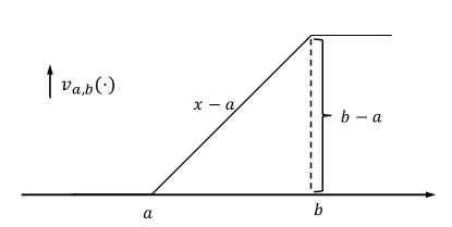
Figure 2.1. The generating dipole function $\left\{v_{a,b}\right\}$ indexed by pairs $a,b$ such that $a<b$. Compare with 3.1 below.

Induced metrics

For a general p.d. kernel $K$ on $X\times X$, there is an induced metric on $X$,

$$d_{K}:X\times X\rightarrow\mathbb{R}_{+}$$

defined as (see e.g., [AJ21])

$$d_{K}\left(x,y\right)=\left\|K\left(\cdot,x\right)-K\left(\cdot,y\right)\right\|_{\mathscr{H}_{K}}^{2}.$$ (2.10)

In particular,

$$d_{K}\left(x,y\right)=K\left(x,x\right)+K\left(y,y\right)-2\Re\left\{K\left(x,y\right)\right\}.$$

Note that $d_{K}^{1/2}$ is also a metric on $X\times X$.

Example 2.5.

For $K\left(x,y\right)=x\wedge y$ on $\mathbb{R}\times\mathbb{R}$ as in (2.4),

$$\left\|K\left(\cdot,s\right)-K\left(\cdot,t\right)\right\|_{\mathscr{H}_{K}}^{2} =\left\|\left(\cdot\wedge s\right)^{\prime}-\left(\cdot\wedge t\right)^{\prime}\right\|_{L^{2}}^{2}$$

$$=\left\|\chi_{\left[0,s\right]}-\chi_{\left[0,t\right]}\right\|_{L^{2}}^{2}$$

$$=\left|s-t\right|.$$

The results below deal with a general framework of pairs of sets $X$ and $Y$, each equipped with a positive definite kernel, $K$ resp., $L$, $K$ on $X$, and $L$ on $Y$. With view to realization of feedforward Neural Network-functions, we will present an explicit framework (see (2.11) and (2.20)) which allows us to pass from (nonlinear) functions $f:X\rightarrow Y$ to linear operators $T_{f}$ acting between the respective RKHSs $\mathscr{H}_{K}$ and $\mathscr{H}_{L}$. This will be a representation in the sense that composition of functions will map into products of the corresponding linear operators. Some care must be exercised as the linear operators $T_{f}$ will in general be unbounded. Nonetheless, we shall show that the operators still fall in a class where spectral resolutions are available, see 2.11 and 2.12.

Theorem 2.6.

Consider p.d. kernels $X\times X\xrightarrow{\;K\;}\mathbb{R}$ and $Y\times Y\xrightarrow{\;L\;}\mathbb{R}$. Let $f:X\rightarrow Y$ be Lipschitz continuous with respect to the induced metrics $d_{K},d_{L}$, i.e.,

$$d_{L}\left(f\left(x\right),f\left(y\right)\right)\leq c_{f}d_{K}\left(x,y\right),\quad x,y\in X,$$

for some constant $c_{f}$. Define the operator $T_{f}:\mathscr{H}_{K}\rightarrow\mathscr{H}_{L}$ by

$$T_{f}\left(K_{x}\right)\left(y\right)=L\left(f\left(x\right),y\right)$$

and extend it by linearity and density.

Then, for any fixed $c\in Y$, the function

$$F_{f}:X\rightarrow\mathbb{R},\quad F_{f}\left(x\right):=L\left(f\left(x\right),c\right)$$ (2.11)

is in the RKHS $\mathscr{H}_{K}$ if, and only if

$$L_{c}\in dom(T_{f}^{*}),$$ (2.12)

the domain of the adjoint operator.

Moreover,

$$F_{f,y}\left(x\right) :=L\left(f\left(x\right),y\right)\in\mathscr{H}_{K},\;\forall y\in Y$$

$$\Updownarrow$$

$$T_{f}\> \text{is closable}.$$

(See also 2.8.)

Proof.

Let the setting be as in the statement of the theorem, i.e., $X\xrightarrow{\;f\;}Y$ assumed continuous with respect to the two metrics, $d_{K}$ on $X$ and $d_{L}$ on $Y$; so in particular, for pairs of points $x_{1},x_{2}\in X$, we have

$$d_{K}\left(x_{1},x_{2}\right) =\left\|K\left(\cdot,x_{1}\right)-K\left(\cdot,x_{2}\right)\right\|_{\mathscr{H}_{K}}^{2}$$ (2.13)

$$=K\left(x_{1},x_{1}\right)+K\left(x_{2},x_{2}\right)-2K\left(x_{1},x_{2}\right).$$ (2.14)

We further fix a point $c\in Y$, and set $F=F_{f,c}$, specified as follows:

$$F\left(x\right)=L\left(f\left(x\right),c\right),\;\text{for all $x\in X$,}$$

so $F:X\rightarrow\mathbb{R}_{+}\cup\left\{0\right\}$.

Now, for every $N$, and every subset $S_{N}=\left(x_{1},x_{2},\dots,x_{N}\right)\subset X$, consider the following matrix operations (in $N$ dimensions):

$$\underset{\text{column vectors}}{\underbrace{F\big{|}_{N}:=\begin{bmatrix}F\left(x_{1}\right)\\ \vdots\\ F\left(x_{N}\right)\end{bmatrix}}},\;\text{and}\quad\underset{\text{matrix of a rank-1 operator}}{\underbrace{Q_{N}:=\left|F\big{|}_{N}\left\rangle\right\langle F\big{|}_{N}\right|}},$$ (2.15)

i.e., the rank-1 operator on $\mathbb{R}^{N}$ written in Dirac’s notation, defined as

$$Q_{N}\left(\xi\right)=\left\langle F_{N},\xi\right\rangle F_{N}$$ (2.16)

for all $\xi\in\mathbb{R}^{N}$. Set

$$K_{N}:=\left(K\left(x_{i},x_{j}\right)\right)_{i,j=1}^{N}=\begin{bmatrix}K\left(x_{1},x_{1}\right)&\cdots&K\left(x_{1},x_{N}\right)\\ \vdots&\ddots&\vdots\\ K\left(x_{N},x_{1}\right)&\cdots&K\left(x_{N},x_{N}\right)\end{bmatrix},$$ (2.17)

a sample matrix.

For the convex cone of all positive definite $N\times N$ matrices, we introduce the following familiar ordering, $K\ll_{C}K^{\prime}$ iff (Def.) $\exists C<\infty$ such that

$$\xi^{T}K_{N}\xi\leq C\xi^{T}K^{\prime}_{N}\xi\;\text{for all }\xi\in\mathbb{R}^{N}.$$ (2.18)

Now an application of 2.1 above shows that the assertion in the theorem is equivalent to the existence of a finite constant $C$ (independent of $S_{N}=\left(x_{i}\right)_{i=1}^{N}$) satisfying $Q_{N}\ll_{C}K_{N}$, i.e., the estimate

$$\left|\sum_{i}\xi L\left(f\left(x_{i}\right),c\right)\right|^{2}\leq C\sum_{i}\sum_{j}\xi_{i}K\left(x_{i},x_{j}\right)\xi_{j}$$ (2.19)

holds for all $N$, all $S_{N}=\left\{x_{i}\right\}_{i=1}^{N}$, and all $\xi\in\mathbb{R}^{N}$. We get this from the assumption on $f$ in the theorem. See details below. ∎

Summary of 2.6: Start with $K$ p.d. on $X\times X$, $L$ p.d. on $Y\times Y$, and $f:X\rightarrow Y$. We introduce the metrics $d_{K}$ on $X$, and $d_{L}$ on $Y$, and we consider $f$ continuous, or Lipchitz. To get the desired conclusion

$$\left(x\longmapsto L\left(f\left(x\right),y\right)\right)\in\mathscr{H}_{K},$$

we must introduce an operator $T_{f}:\mathscr{H}_{K}\rightarrow\mathscr{H}_{L}$. The right choice is

$$L_{y}\in dom(T_{f}^{*}).$$

See details below:

Fixing two kernels $K$ and $L$, assumed p.d. on $X\times X$, and on $Y\times Y$. Pass to the corresponding RKHS $\mathscr{H}_{K}$ and $\mathscr{H}_{L}$.

Problem.

Find conditions on functions $X\xrightarrow{\;f\;}Y$ with the property that, for $\forall y\in Y$, then the induced function

$$\underset{F_{f,y}\left(\cdot\right)\text{ as a function on $X$}}{\underbrace{\left(X\ni x\longmapsto L\left(f\left(x\right),y\right)\right)}}\in\mathscr{H}_{K}.$$ (2.20)

The argument stressed below is via dual operators (bounded)

$$\lx@xy@svg{\hbox{\raise 0.0pt\hbox{\kern 9.32834pt\hbox{\ignorespaces\ignorespaces\ignorespaces\hbox{\vtop{\kern 0.0pt\offinterlineskip\halign{\entry@#!@&&\entry@@#!@\cr&&\crcr}}}\ignorespaces{\hbox{\kern-9.32834pt\raise 0.0pt\hbox{\hbox{\kern 0.0pt\raise 0.0pt\hbox{\hbox{\kern 3.0pt\raise 0.0pt\hbox{$\textstyle{\mathscr{H}_{K}\ignorespaces\ignorespaces\ignorespaces\ignorespaces\ignorespaces}$}}}}}}}\ignorespaces\ignorespaces\ignorespaces\ignorespaces\ignorespaces{}{}{}{{}{}{}{}{}{}{}{}{}{}{}{}{}{}{}{}}{}\ignorespaces\hbox{\hbox{\kern 0.0pt\raise 0.0pt\hbox{{}{}{{}}{{}{}{}}{}}}}\ignorespaces{}\ignorespaces{}{}{}{{}{}}\ignorespaces\ignorespaces{\hbox{\kern 29.2661pt\raise 22.07503pt\hbox{{}\hbox{\kern 0.0pt\raise 0.0pt\hbox{\hbox{\kern 3.0pt\hbox{\hbox{\kern 0.0pt\raise-1.30833pt\hbox{$\scriptstyle{T_{f}}$}}}\kern 3.0pt}}}}}}\ignorespaces{}{}{}{{}{}{}{}{}{}{}{}{}{}{}{}{}{}{}{}{}{}{}{}}{\hbox{\kern 63.32863pt\raise 6.60085pt\hbox{\hbox{\kern 0.0pt\raise 0.0pt\hbox{\lx@xy@tip{1}\lx@xy@tip{-1}}}}}}\ignorespaces\hbox{\hbox{\kern 0.0pt\raise 0.0pt\hbox{{}{}{}{{}}{{}{}{}\lx@xy@spline@}{}}}}\ignorespaces{}\ignorespaces\hbox{\hbox{\kern 0.0pt\raise 0.0pt\hbox{{}{}{{}}{{}{}{}}{}}}}\ignorespaces{}{\hbox{\kern 33.32834pt\raise 0.0pt\hbox{\hbox{\kern 0.0pt\raise 0.0pt\hbox{\hbox{\kern 3.0pt\raise 0.0pt\hbox{$\textstyle{}$}}}}}}}{\hbox{\kern 63.32834pt\raise 0.0pt\hbox{\hbox{\kern 0.0pt\raise 0.0pt\hbox{\hbox{\kern 3.0pt\raise 0.0pt\hbox{$\textstyle{\mathscr{H}_{L}\ignorespaces\ignorespaces\ignorespaces\ignorespaces\ignorespaces}$}}}}}}}\ignorespaces\ignorespaces\ignorespaces\ignorespaces\ignorespaces{}{}{}{{}{}{}{}{}{}{}{}{}{}{}{}{}{}{}{}}{}\ignorespaces\hbox{\hbox{\kern 0.0pt\raise 0.0pt\hbox{{}{}{{}}{{}{}{}}{}}}}\ignorespaces{}\ignorespaces{}{}{}{{}{}}\ignorespaces\ignorespaces{\hbox{\kern 29.2661pt\raise-22.5403pt\hbox{{}\hbox{\kern 0.0pt\raise 0.0pt\hbox{\hbox{\kern 3.0pt\hbox{\hbox{\kern 0.0pt\raise-1.77362pt\hbox{$\scriptstyle{T_{f}^{*}}$}}}\kern 3.0pt}}}}}}\ignorespaces{}{}{}{{}{}{}{}{}{}{}{}{}{}{}{}{}{}{}{}{}{}{}{}{}}{\hbox{\kern 6.20372pt\raise-4.91432pt\hbox{\hbox{\kern 0.0pt\raise 0.0pt\hbox{\lx@xy@tip{1}\lx@xy@tip{-1}}}}}}\ignorespaces\hbox{\hbox{\kern 0.0pt\raise 0.0pt\hbox{{}{}{}{{}}{{}{}{}\lx@xy@spline@}{}}}}\ignorespaces{}\ignorespaces\hbox{\hbox{\kern 0.0pt\raise 0.0pt\hbox{{}{}{{}}{{}{}{}}{}}}}\ignorespaces{}\ignorespaces}}}}\ignorespaces; \textstyle{\mathscr{H}_{K}\ignorespaces\ignorespaces\ignorespaces\ignorespaces\ignorespaces} \scriptstyle{T_{f}} \textstyle{\mathscr{H}_{L}\ignorespaces\ignorespaces\ignorespaces\ignorespaces\ignorespaces} \scriptstyle{T_{f}^{*}} \textstyle{\mathscr{H}_{K}\ignorespaces\ignorespaces\ignorespaces\ignorespaces\ignorespaces} \scriptstyle{T_{f}} \textstyle{\mathscr{H}_{L}\ignorespaces\ignorespaces\ignorespaces\ignorespaces\ignorespaces} \scriptstyle{T_{f}^{*}}$$

but the unbounded case is also interesting.

Some remarks on the definition of the operator $T_{f}:\mathscr{H}_{K}\rightarrow\mathscr{H}_{L}$ in the case when no additional assumptions are placed on $X\xrightarrow{\;f\;}Y$.

We define

$$T_{f}\left(K_{x}\right)\left(y\right)=L\left(f\left(x\right),y\right);$$

and so we extend $T_{f}$ to linear combinations:

$$\mathscr{D}_{K}:=\underset{\text{function on $X$}}{\big{\{}\underbrace{\sum_{i}c_{i}K_{x_{i}}}\big{\}}}\xrightarrow{\quad T_{f}\quad}\underset{\text{function on $Y$}}{\underbrace{\sum_{i}c_{i}L\left(f\left(x_{i}\right),\cdot\right)}}.$$ (2.21)

But to make sense of (2.21) so it is well defined, we must be careful with equivalence classes.

If $f:X\rightarrow Y$ is a general function, the (generalized) operator (2.21) may be non-closable. However, we can still define the adjoint $T_{f}^{*}$ , but its domain might be “small”.

Set

$$\mathscr{D}_{K}:=span\left\{K_{x}\right\}_{x\in X},$$ (2.22)

then (Definition) a vector $\psi\in\mathscr{H}_{L}$ is in $dom(T_{f}^{*})$ iff $\exists C_{\psi}<\infty$ s.t.

$$\left|\left\langle T_{f}\varphi,\psi\right\rangle_{\mathscr{H}_{L}}\right|\leq C_{\psi}\left\|\varphi\right\|_{\mathscr{H}_{K}},\quad\forall\varphi\in\mathscr{D}_{K}.$$ (2.23)

We then set $T_{f}^{*}\psi=$ the solution to

$$\left\langle T_{f}\varphi,\psi\right\rangle_{\mathscr{H}_{L}}=\left\langle\varphi,T_{f}^{*}\psi\right\rangle_{\mathscr{H}_{K}},\quad\forall\varphi\in\mathscr{D}_{K}.$$ (2.24)

Let $K,L,f$ be as specified, and assume for some $y\in Y$, that we have $L_{y}\in dom(T_{f}^{*})$, then (2.24) for $L_{y}\in\mathscr{H}_{L}\xrightarrow{\;T_{f}^{*}\;}\mathscr{H}_{K}$, $\varphi=K_{x}$, $\psi=L_{y}$ yields

$$x\longmapsto T_{f}^{*}\left(L_{y}\right)\left(x\right)=L\left(f\left(x\right),y\right)\in\mathscr{H}_{K}.$$

So the conclusion in 2.6 that

$$\left(x\longmapsto L\left(f\left(x\right),y\right)\right)\in\mathscr{H}_{K}$$ (2.25)

holds iff $L_{y}\in dom(T_{f}^{*})$.

In this case there are no difficulties with (2.21) and we get a dual pair $T_{f}$ and $T_{f}^{*}$,

$$\left\langle T_{f}\varphi,\psi\right\rangle_{\mathscr{H}_{L}}=\left\langle\varphi,T_{f}^{*}\psi\right\rangle_{\mathscr{H}_{K}}$$ (2.26)

for $\forall\varphi\in\mathscr{D}_{K}$, and $\psi\in\mathscr{D}_{L}$, .

Setting $\varphi=K_{x}$, and $\psi=L_{y}$, (2.26) implies

$$T_{f}^{*}\left(L_{y}\right)\left(x\right)=L\left(f\left(x\right),y\right)=\left(T_{f}\left(K_{x}\right)\right)\left(y\right).$$ (2.27)

But the previous condition $L_{y}\in dom(T_{f}^{*})$ (compare (2.26)) amounts to the assertion that $T_{f}^{*}\left(L_{y}\right)\in\mathscr{H}_{K}$, and by (2.27), this is then the conclusion for 2.6.

Corollary 2.7 (composition operators).

Let $X$, $Y$, $K$ and $L$ be as specified above; in particular, $K$ is a fixed p.d. kernel on $X\times X$, and the RKHS $\mathscr{H}_{K}$ is a Hilbert space of scalar valued functions on $X$. Similarly, $\mathscr{H}_{L}$ is a Hilbert space of scalar valued functions on $Y$. Both $\mathscr{H}_{K}$ and $\mathscr{H}_{L}$ satisfy the defining axioms for RKHSs; see 2.1 above. As noted, every function $f$, $X\xrightarrow{\;f\;}Y$, induces a linear operator

$$\mathscr{H}_{K}\xrightarrow{\;T_{f}\;}\mathscr{H}_{L},$$ (2.28)

with dense domain $\mathscr{D}_{K}$; see the statement of 2.6. For the adjoint operator $T_{f}^{*}$,

$$\mathscr{H}_{L}\xrightarrow{\;T_{f}^{*}\;}\mathscr{H}_{K},$$ (2.29)

we have the following: For a function $\psi$ in $\mathscr{H}_{L}$, the two characterizations (2.30) and (2.31) hold:

$$\psi\in dom(T_{f}^{*})$$ (2.30)

$$\Updownarrow$$

$$\psi\circ f\in\mathscr{H}_{K}.$$ (2.31)

In the affirmative,

$$T_{f}^{*}\left(\psi\right)=\psi\circ f:X\rightarrow\mathbb{R},$$ (2.32)

i.e., $T_{f}^{*}$ is the composition operator.

Proof.

(2.30)$\Rightarrow$(2.31). Assume (2.30), we then apply (2.23), and get $C_{\psi}<\infty$ with:

$$\left|\sum_{i}c_{i}\left(T_{f}^{*}\left(\psi\right)\right)\left(x_{i}\right)\right|^{2}\leq C_{\psi}\sum_{i}\sum_{j}c_{i}c_{j}K\left(x_{i},x_{j}\right).$$ (2.33)

But

$$T_{f}^{*}\left(\psi\right)\left(x_{i}\right) =\left\langle K_{x_{i}},T_{f}^{*}\left(\psi\right)\right\rangle_{\mathscr{H}_{K}}$$ (2.34)

$$=\left\langle T_{f}\left(K_{x_{i}}\right),\psi\right\rangle_{\mathscr{H}_{L}}$$

$$=\left\langle L\left(f\left(x_{i}\right),\cdot\right),\psi\right\rangle_{\mathscr{H}_{L}}$$

$$=\psi\left(f\left(x_{i}\right)\right),$$

where we used the RKHS property for $\mathscr{H}_{L}$ in the last step. Substitution into (2.33) yields

$$\left|\sum_{i}c_{i}\psi\left(f\left(x_{i}\right)\right)\right|^{2}\leq C_{\psi}\sum_{i}\sum_{j}c_{i}c_{j}K\left(x_{i},x_{j}\right),$$ (2.35)

and, so by 2.1 applied to $F=\psi\circ f$, conclusion in (2.31) follows.

(2.31)$\Rightarrow$(2.30). Assume (2.31), we then reverse the above reasoning to get

$$\Big{|}\Big{\langle}T_{f}\underset{\in\mathscr{D}_{K}}{\underbrace{\left(\sum_{i}c_{i}K_{x_{i}}\right)}},\psi\Big{\rangle}_{\mathscr{H}_{L}}\Big{|}\leq\sqrt{C_{\psi}}\left\|\sum_{i}c_{i}K_{x_{i}}\right\|_{\mathscr{H}_{K}}$$ (2.36)

which states that $\psi\in dom(T_{f}^{*})$, which is condition (2.30). Now combine this with (2.34), and we conclude that (2.32) is satisfied for $\psi$, i.e., that $T_{f}^{*}\psi=\psi\circ f$ holds. ∎

2.1. Basis approach

Let $X,Y,K,L,f$ be as usual, and define $T_{f}:\mathscr{H}_{K}\rightarrow\mathscr{H}_{L}$. Since $K$ is p.d. on $X\times X$, the RKHS $\mathscr{H}_{K}$ allows an ONB $\left\{h_{i}\right\}_{i\in\mathbb{N}}$, $h_{i}\in\mathscr{H}_{K}$; by general theory, we get the pointwise formula:

$$K\left(x_{1},x_{2}\right)=\sum_{i\in\mathbb{N}}h_{i}\left(x_{1}\right)h_{i}\left(x_{2}\right).$$ (2.37)

Then our condition in 2.6 is equivalent to the following:

$$\left(X\ni x\longmapsto L\left(f\left(x\right),y\right)\right)\in\mathscr{H}_{K}$$ (a)

$$\Updownarrow$$

$$\sum_{i\in\mathbb{N}}\left|\left(T_{f}\left(h_{i}\right)\right)\left(y\right)\right|^{2}<\infty.$$ (b)

Proof.

$\left(a\right)\Rightarrow\left(b\right)$ is detailed below; but the converse implication will follow by the same argument. So by $\left(a\right)$, $L_{y}\in dom(T_{f}^{*})$ and therefore:

$$T_{f}^{*}\left(L_{y}\right)\left(\cdot\right)\in\mathscr{H}_{K}.$$ (2.38)

Since $\left\{h_{i}\right\}$ is an ONB in $\mathscr{H}_{K}$,

$$\sum_{i}\Big{|}\big{\langle}h_{i},\underset{\in\mathscr{H}_{K}}{\underbrace{T_{f}^{*}\left(L_{y}\right)}}\big{\rangle}\Big{|}^{2}=\left\|T_{f}^{*}\left(L_{y}\right)\right\|_{\mathscr{H}_{K}}^{2}<\infty.$$ (2.39)

But from the $\text{LHS}_{\left(\ref{eq:bd3}\right)}$:

$$\left\langle h_{i},T_{f}^{*}\left(L_{y}\right)\right\rangle_{\mathscr{H}_{K}}=\left\langle T_{f}\left(h_{i}\right),L_{y}\right\rangle_{\mathscr{H}_{L}}=\left(T_{f}\left(h_{i}\right)\right)\left(y\right),$$

and $\left(b\right)$ follows. ∎

Key Question: When is $F_{f,y}\left(\cdot\right)\in\mathscr{H}_{K}$? The cleanest answer to the question of what functions $X\xrightarrow{\;f\;}Y$ have the property that

$$F_{f,y}\left(x\right)=L\left(f\left(x\right),y\right)\text{ is in $\mathscr{H}_{K}$ }$$ (2.40)

is this:

Theorem 2.8.

Let $K,L$ and $f$ be given, then

$$F_{f,y}\>\text{in }\left(\ref{eq:cd1}\right)\;\text{is in $\mathscr{H}_{K}\Longleftrightarrow L_{y}\in$dom($T_{f}^{*}$),}$$ (2.41)

where the operator $T_{f}:\mathscr{H}_{K}\rightarrow\mathscr{H}_{L}$ is given by

$$T_{f}\left(K_{x}\right):=L\left(f\left(x\right),\cdot\right).$$

Moreover, (2.41) holds for all $y\in Y\Longleftrightarrow T_{f}$ is closable.

2.2. Dual pairs of operators

Consider a symmetric pair of operators with dense domains:

($T=T_{f}$, since it will depend on $f$) where

$$span\left\{K_{x}\right\}_{x\in X}\>\text{is dense in $\mathscr{H}_{K}$}$$ (2.42)

and

$$span\left\{L_{y}\right\}_{y\in Y}\>\text{is dense in $\mathscr{H}_{L}$}$$ (2.43)

such that

$$K_{x} \in dom(T_{f}),\;\text{and}$$ (2.44)

$$L_{y} \in dom(T_{f}^{*})$$ (2.45)

where “$dom$” denotes the respective operator domains.

Note.

We note that

$$T_{f}\left(K_{x}\right)\left(\cdot\right)=L\left(f\left(x\right),\cdot\right)\in\mathscr{H}_{L}$$

is always well defined, with dense domain, but the secret is $T_{f}^{*}.$

Also note that (2.45) is the condition in 2.6.

Let $f:X\rightarrow Y$ be as before, and the two p.d. kernels $K$ and $L$ are fixed. We then introduce the corresponding (densely defined) operator $T_{f}:\mathscr{H}_{K}\rightarrow\mathscr{H}_{L}$ by setting

$$T_{f}\left(K_{x}\right)=L\left(f\left(x\right),\cdot\right)\in\mathscr{H}_{L}.$$ (2.46)

Notation and convention. $K_{x}\left(\cdot\right)$ is the kernel function in $\mathscr{H}_{K}$ as usual:

$$K_{x}\left(t\right) =K\left(x,t\right),\;\forall t\in X\>\text{and similarly,}$$ (2.47)

$$L_{y}\left(u\right) =L\left(y,u\right),\;\forall u\in Y.$$ (2.48)

Lemma 2.9.

When $L_{y}\in dom(T_{f}^{*})$ then

$$\left(T_{f}^{*}\left(L_{y}\right)\right)\left(x\right)=L\left(f\left(x\right),y\right)\;\text{on $X$,}$$ (2.49)

equivalently,

$$T_{f}^{*}\left(L_{y}\right)\left(\cdot\right)=L\left(f\left(\cdot\right),y\right)\;\text{on $X$.}$$ (2.50)

Proof of (2.49).

The conclusion (2.49) is equivalent to the following assertion:

The conclusion (2.49) follows since the respective kernel functions span dense subspaces. ∎

Recall,

$$\text{the function }x \longmapsto F_{f,y}\left(x\right)=L\left(f\left(x\right),y\right)\in\mathscr{H}_{K}$$

$$\Updownarrow$$

$$L_{y} \in dom(T_{f}^{*}).$$

Assume that $L_{y}\in dom(T_{f}^{*})$ , then apply the condition for functions in $\mathscr{H}_{K}$ to $F_{f,y}\left(\cdot\right)$, so $\forall n$, $\forall\left(x_{i}\right)_{1}^{n}$, $\forall\left(c_{i}\right)_{1}^{n}$, $c_{i}\in\mathbb{R}$:

$$\left|\sum_{i}c_{i}F_{f,y}\left(x_{i}\right)\right|^{2} = \left|\sum_{i}c_{i}L\left(f\left(x_{i}\right),y\right)\right|^{2}$$

$$\leq \left|\left\langle\sum_{i}c_{i}K_{x_{i}},T_{f}^{*}\left(L_{y}\right)\right\rangle_{\mathscr{H}_{K}}\right|^{2}$$

$$\underset{\text{Schwarz}}{\leq} \left\|\sum_{i}c_{i}K_{x_{i}}\right\|_{\mathscr{H}_{K}}^{2}\left\|T_{f}^{*}\left(L_{y}\right)\right\|_{\mathscr{H}_{K}}^{2}$$

$$= \sum_{i}\sum_{j}c_{i}c_{j}K\left(x_{i},x_{j}\right)\left\|T_{f}^{*}\left(L_{y}\right)\right\|_{\mathscr{H}_{K}}^{2}.$$

Lemma 2.10.

The implication below is both directions:

$$X\ni x\longmapsto L\left(f\left(x\right),y\right)\in\mathscr{H}_{K}\;\text{for $\forall y$}$$

$$\Updownarrow$$

$$\text{the condition in $\left(\ref{thm:mc}\right)$ is satisfied}.$$

Even if we fix $y\in Y$, then

$$L_{y}\in dom(T_{f}^{*})\Longleftrightarrow\left(x\longmapsto L\left(f\left(x\right),y\right)\right)\in\mathscr{H}_{K}.$$ (2.51)

Proof sketch.

By definition, $L_{y}\in dom(T_{f}^{*})$, $\exists C_{y}<\infty$ $\Longleftrightarrow$

$$\left|\left\langle T_{f}\varphi,L_{y}\right\rangle_{\mathscr{H}_{L}}\right|=\left|\left(T_{f}\left(\varphi\right)\right)\left(y\right)\right|\leq C_{y}\left\|\varphi\right\|_{\mathscr{H}_{K}}$$

holds for $\forall\varphi\in span\left\{K_{x}\right\}_{x\in X}.$ But

$$T_{f}\left(K_{x}\right)\left(y\right) =L\left(f\left(x\right),y\right),\;\text{and}$$ (2.52)

$$\Big{|}\sum_{i}c_{i}\underset{F_{f,y}\left(x_{i}\right)}{\underbrace{L\left(f\left(x_{i}\right),y\right)}}\Big{|} {}^{2}=\left|\Big{\langle}\sum_{i}c_{i}K_{x_{i}},T_{f}^{*}\left(L_{y}\right)\Big{\rangle}_{\mathscr{H}_{K}}\right|^{2}$$ (2.53)

$$\leq\left\|T_{f}^{*}\left(L_{y}\right)\right\|_{\mathscr{H}_{K}}^{2}\underset{<\infty}{\underbrace{\sum_{i}\sum_{j}c_{i}c_{j}K\left(x_{i},x_{j}\right)}}$$ (2.54)

and so by the basic lemma for $\mathscr{H}_{K}$ (see the proof of 2.6), we conclude that functions $F_{f,y}\in\mathscr{H}_{K}$, i.e., $\left(x\longmapsto L\left(f\left(x\right),y\right)\right)\in\mathscr{H}_{K}$.

Conclusion: the bi-implication $\Longleftrightarrow$ in (2.51) is valid. ∎

2.3. Functions and Operators

In general if $T:\mathscr{H}_{1}\rightarrow\mathscr{H}_{2}$ is an operator with dense domain $\mathscr{D}\subset\mathscr{H}_{1}$, where $\mathscr{H}_{i}$, $i=1,2$, are two Hilbert spaces, we know that $T$ is closable $\Longleftrightarrow$ $T^{*}$ is densely defined, i.e., iff $dom(T^{*})$ is dense in $\mathscr{H}_{2}$ (see e.g., [JT21]). So we apply this to $T=T_{f}$, $\mathscr{H}_{1}=\mathscr{H}_{K}$, $\mathscr{H}_{2}=\mathscr{H}_{L}$, and the condition in 2.6 holds $\Longleftrightarrow$ $L_{y}\in dom(T_{f}^{*})$ $\forall y\in Y$. Since $span\left\{L_{y}\right\}_{y\in Y}$ is dense in $\mathscr{H}_{L}$, the condition in 2.6 $\Longrightarrow$ $T_{f}$ is closable.

Given $K$ and $L$ as above, introduce

$$\mathscr{F}_{ub}\left(K,L\right) =\left\{f:T_{f}\text{ is closable}\right\},\;\text{and}$$ (2.55)

$$\mathscr{F}_{b}\left(K,L\right) =\left\{f:T_{f}\text{ is bounded from $\mathscr{H}_{K}$ into $\mathscr{H}_{L}$}\right\}.$$ (2.56)

In both cases, the operators $T=T_{f}$ depends on the choice of function $X\xrightarrow{\;f\;}Y$, but the two conditions (2.55) and (2.56) are different:

$$\left(T_{f}\left(K_{x}\right)\right)\left(y\right)=L\left(f\left(x\right),y\right)=\left(\left(T_{f}\right)^{*}\left(L_{y}\right)\right)\left(x\right),$$ (2.57)

for all $x\in X$, and $y\in Y$. See details below:

Some general comments about the operator $T_{f}:\mathscr{H}_{K}\rightarrow\mathscr{H}_{L}$. As before, $K$ and $L$ are fixed p.d. kernels, and $f:X\rightarrow Y$ is a function. We need to understand the conclusion from 2.6, i..e, when is

$$\left(X\ni x\longmapsto L\left(f\left(x\right),y\right)\right)\in\mathscr{H}_{K}\;\text{for all $y\in Y$}?$$ (2.58)

Answer: (2.58) $\Longleftrightarrow$ $L_{y}\in dom(T_{f}^{*})$.

Note that then the function in (2.58) is $T_{f}^{*}\left(L_{y}\right)$; see (2.57). But note that, starting with a function $X\xrightarrow{\;f\;}Y$, there are requirements for having (2.57) yield a well defined linear operator $T_{f}$ with dense domain in $\mathscr{H}_{K}$, s.t.

$$T_{f}\left(K_{x}\right)\left(\cdot\right)=L\left(f\left(x\right),\cdot\right).$$ (2.59)

The case when $T_{f}$ is bounded is easy since then $dom(T_{f}^{*})=\mathscr{H}_{L}$. Notationally, $L\left(f\left(x\right),\cdot\right)\in L_{f\left(x\right)}\in\mathscr{H}_{L}$, but we must also verify the implicit kernel function for all finite sums:

$$\sum_{i}\sum_{j}c_{i}c_{j}K\left(x_{i},x_{j}\right)=0\Longrightarrow\sum_{i}\sum_{j}c_{i}c_{j}L\left(f\left(x_{i}\right),f\left(x_{j}\right)\right)=0.$$

2.4. The case when $K=L$

As demonstrated in 3 below, for applications to multi-level NNs, the recursive constructions simplify when the same p.d. kernel $K$ is used at each level. Hence below, we specialize to the case when $X=Y$, and $K=L$; see the setting in Theorems 2.6 and 2.8.

Theorem 2.11.

Consider a positive definite kernel $K$ on $X\times X$, and the corresponding RKHS $\mathscr{H}_{K}$, i.e., the Hilbert completion of $\left\{K_{x}\right\}_{x\in X}$ where $K_{x}:=K\left(\cdot,x\right)$. Fix a function $X\xrightarrow{\;f\;}X$ with the property (see 2.6) that

$$\left(X\ni x\longmapsto K\left(f\left(x\right),y\right)\right)\in\mathscr{H}_{K}\;\text{for all $y\in X$.}$$ (2.60)

Hence, the operator $T_{f}:\mathscr{H}_{K}\rightarrow\mathscr{H}_{K}$ defined by

$$T_{f}\left(K\left(\cdot,y\right)\right):=K\left(f\left(\cdot\right),y\right)$$ (2.61)

is a densely defined operator from $\mathscr{H}_{K}$ into $\mathscr{H}_{K}$, with domain

$$\mathscr{D}_{K}:=span\left\{K_{x}\right\}_{x\in X}.$$ (2.62)

1. Then the closure of $T_{f}$ (also denoted $T_{f}$) is well defined and normal, i.e., the two operators $T_{f}$ and $T_{f}^{*}$ commute.

2. In particular, $T_{f}$ has a projection-valued spectral resolution, i.e., there is a projection-valued measure $Q\left(\cdot\right)$ on $\mathscr{B}_{\mathbb{C}}\left(=\text{the Borel subsets in $\mathbb{C}$}\right)$ such that

   $$T_{f}=\int_{spect\left(T_{f}\right)}\lambda\,Q\left(d\lambda\right):\mathscr{D}_{K}\rightarrow\mathscr{H}_{K}.$$ (2.63)

Proof.

Note that part (2) follows from (1) and the Spectral Theorem for normal operators (in the Hilbert space $\mathscr{H}_{K}$.)

Part (1). When the operator $T_{f}^{*}$ is introduced, we get the following commutativity:

Figure 2.2. Commutativity of $T_{f}$ and $T_{f}^{*}$.

which is the desired conclusion (1). ∎

Given a function $f:X\rightarrow X$ as in 2.11. Below we make use of the corresponding projection valued measure $Q^{\left(f\right)}$ from 2.11 in order to establish an assignment from pairs $(x,y)$ of points in $X$, into systems of complex measures $\mu_{\left(x,y\right)}$ on the spectrum of $T_{f}$. In this assignment, $n$-fold composition-iteration of the function $f$ yields the $n$th moment of each of the measures $\mu_{\left(x,y\right)}$.

Corollary 2.12.

Let $K,X$ and $f$ be as specified in 2.11, and let $Q=Q^{\left(K,f\right)}\left(\cdot\right)$ be the corresponding projection valued measure in (2.63). Then for every pair $x,y\in X$, we get a corresponding Borel measure

$$\mu_{x,y}^{\left(f\right)}\left(B\right)=\left\langle K_{x},Q\left(B\right)K_{y}\right\rangle_{\mathscr{H}_{K}}=\left(Q\left(B\right)\left(K_{y}\right)\right)\left(x\right),$$ (2.64)

for all $B\in\mathscr{B}_{\mathbb{C}}$. Inductively, setting

$$f^{\circ n}=\underset{\text{$n$ fold}}{\underbrace{f\circ\cdots\circ f}}$$

we arrive at the following moment formula for the respective complex measures:

$$\mu_{f^{\circ n}\left(x\right),y}^{\left(f\right)}\left(B\right)=\int_{B}\lambda^{n}\,\mu_{x,y}^{\left(f\right)}\left(d\lambda\right).$$ (2.65)

We now turn to the role of multipliers in the RKHS $\mathscr{H}_{K}$.

Definition 2.13.

A scalar valued function $\varphi$ on $X$ is said to be a multiplier for $\mathscr{H}_{K}$ iff one of the two equivalent conditions hold:

1. The multiplication operator $M_{\varphi}$ acting on $\mathscr{H}_{K}$ via $M_{\varphi}F=\varphi F$ (via pointwise product) leaves $\mathscr{H}_{K}$ invariant.

2. We have the following identity for the adjoint operator:

   $$M_{\varphi}^{*}\left(K_{x}\right)=\varphi\left(x\right)K_{x}\;\text{for all $x\in X$}$$ (2.66)

   where $K_{x}$ denotes the kernel function $K_{x}=K\left(\cdot,x\right)$.

Remark 2.14.

The equivalence of (1) and (2) follows from the standard reference on RKHSs; see e.g., [JT21].

Theorem 2.15.

Let $K$ be a fixed p.d. kernel on $X\times X$, and let $\mathscr{H}_{K}$ be the corresponding RKHS. Let $X\xrightarrow{\;f\;}X$ be a function such that (2.60) holds, i.e., $\left(X\ni x\longmapsto K\left(f\left(x\right),y\right)\right)\in\mathscr{H}_{K}$ for all $y\in X$.

Then for every multiplier $\varphi$ for $\mathscr{H}_{K}$, we have:

$$M_{\left(\varphi\circ f\right)}T_{f}^{*}=T_{f}^{*}M_{\varphi}.$$ (2.67)

Proof.

It is clear that the conclusion (2.67) has the following equivalent form:

$$T_{f}M_{\left(\varphi\circ f\right)}^{*}=M_{\varphi}^{*}T_{f};$$ (2.68)

and below we shall prove (2.68).

Let $f$ and $\varphi$ be as specified in the theorem. We then have the following commutative diagram:

Figure 2.3. Commutative diagram corresponding to (2.68).

In the verification of the assertions in 2.3, we used the conclusions in Theorems 2.6 and 2.8 above. ∎

3. Neural Network-activation functions from p.d. kernels

In the previous section we introduced the use of positive definite kernels, and associated generating function for the NN algorithms. Below we make use of the kernel analysis in design of the generating NN functions.

The next definition makes use of the iterative generation of feedforward functions as in the literature, e.g., [CC21, CKM22, Han16]. The recursive steps used here in the definition and 3.2 below serve as applications of our general framework from Theorems 2.6 and 2.8 above.

Definition 3.1.

Let $K$ be a positive definite kernel on $\mathbb{R}$. An $l$-layer feedforward network with kernel $K$ is a function of the form

$$x\mapsto y_{1}=K\left(A_{1}x+b_{1},c_{1}\right)\mapsto y_{2}=K\left(A_{2}y_{1}+b_{2},c_{2}\right)\mapsto\cdots\\ \cdots\mapsto y_{l}=K\left(A_{l}y_{l-1}+b_{l},c_{l}\right)\mapsto y_{out}=K\left(\left\langle a_{l+1},y_{l}\right\rangle+b_{l+1},c_{l+1}\right)$$

where

• $x\in\mathbb{R}^{n_{0}}$;

• $A_{j}\in\mathbb{R}^{n_{j}\times n_{j-1}}$, $b_{j},c_{j}\in\mathbb{R}^{n_{j}}$ for $j=1,\cdots,l$;

• $a_{l+1}\in\mathbb{R}^{n_{l}}$, $b_{l+1},c_{l+1}\in\mathbb{R}$;

and for vectors $x,y\in\mathbb{R}^{m}$,

$$K\left(x,y\right):=\left[K\left(x_{1},y_{1}\right),\cdots,K\left(x_{m},y_{m}\right)\right].$$

Lemma 3.2.

Let $K\left(x,y\right)=\min\left(x,y\right)$, and $a,b,c,d$ be nonzero constants. Then

1. $K\left(ax+b,c\right)=aK\left(x,a^{-1}\left(c-b\right)\right)+b$;

2. $K\left(K\left(x,a\right),b\right)=K\left(x,K\left(a,b\right)\right)$;

3. $K\left(dK\left(ax+b,c\right)+e,f\right)=daK\left(x,K\left(a^{-1}\left(c-b\right),a^{-1}\left(d^{-1}\left(f-e\right)-b\right)\right)\right)+db+e$.

Proof.

1. $K\left(ax+b,c\right)=\begin{cases}ax+b&x<a^{-1}\left(c-b\right)\\ c&x>a^{-1}\left(c-b\right)\end{cases}$

2. Assume $a<b$, then

   $$K\left(K\left(x,a\right),b\right)=\begin{cases}x&x<a\\ a&x\geq a\end{cases}=K\left(x,a\right).$$

   The case $a>b$ is similar.

3. This follows from (1)–(2):

   $$K\left(dK\left(ax+b,c\right)+e,f\right)$$

   $$= dK\left(K\left(ax+b,c\right),d^{-1}\left(f-e\right)\right)+e$$

   $$= dK\left(aK\left(x,a^{-1}\left(c-b\right)\right)+b,d^{-1}\left(f-e\right)\right)+e$$

   $$= d\left\{aK\left(K\left(x,a^{-1}\left(c-b\right)\right),a^{-1}\left(d^{-1}\left(f-e\right)-b\right)\right)+b\right\}+e$$

   $$= daK\left(K\left(x,a^{-1}\left(c-b\right)\right),a^{-1}\left(d^{-1}\left(f-e\right)-b\right)\right)+db+e$$

   $$= daK\left(x,K\left(a^{-1}\left(c-b\right),a^{-1}\left(d^{-1}\left(f-e\right)-b\right)\right)\right)+db+e$$

∎

In what follows, all the networks are restricted to be defined on compact subsets $\Omega$ in $\mathbb{R}^{d}$, e.g., $\Omega=\left[0,1\right]^{d}$ (hypercubes). This is in consideration of standard normalizations in training neural networks.

In Theorems 3.3 and 3.4, we present in detail the particular relative Reproducing Kernel Hilbert Spaces which have as their respective dipole system (see (3.5)) the generalized ReLu functions illustrated here in Figures 2.1 and 3.1.

Here we specify the kernel $K_{1}$ for Brownian motion $W$ indexed by $\mathbb{R}$. As a result, the corresponding p.d. kernel on $\mathbb{R}\times\mathbb{R}$ is as follows:

$$K_{1}\left(x,y\right)=\begin{cases}\left|x\right|\wedge\left|y\right|=\min\left(\left|x\right|,\left|y\right|\right)&\text{if}\;xy\geq 0\;\text{(so same sign)}\\ 0&\text{if $xy<0,$ so opposite sign.}\end{cases}$$ (3.1)

Proof.

The connection between the kernel $K_{1}$ and the Brownian motion $\left\{W_{x}\right\}_{x\in\mathbb{R}}$ is as follows:

$$K_{1}\left(x,y\right)=\mathbb{E}\left(\left(W_{x}-W_{0}\right)\left(W_{y}-W_{0}\right)\right)$$ (3.2)

for all $x,y\in\mathbb{R}$. The asserted formula (3.1) follows from this, combined with the independence of increments for Brownian motion. ∎

Theorem 3.3.

Let $K_{1}$ be the p.d. kernel (3.1) on $\mathbb{R}\times\mathbb{R}$, with the corresponding RKHS

$$\mathscr{H}_{K_{1}}=\left\{f:f^{\prime}\in L^{2}\right\},\quad\left\|f\right\|_{\mathscr{H}_{K_{1}}}^{2}=\int\left|f^{\prime}\right|^{2}d\lambda_{1}.$$

On $\Omega=\left[0,1\right]^{d}$, consider the p.d. kernel

$$K_{d}\left(x,y\right)=K_{1}\left(x_{1},y_{1}\right)\cdots K_{1}\left(x_{d},y_{d}\right),$$

so that

$$\mathscr{H}_{K_{d}}=\left\{f:\nabla f\in L^{2}\right\},\quad\left\|f\right\|_{\mathscr{H}_{K_{d}}}^{2}=\int\left|\nabla f\right|^{2}d\lambda_{d},$$

where $\lambda_{d}$ denotes the $d$-dimensional Lebesgue measure.

Given $f:\Omega\rightarrow\mathbb{R}$, and a fixed $c\in\mathbb{R}$, set

$$F:\mathbb{R}^{d}\rightarrow\mathbb{R}^{1},\quad F\left(x\right)=K_{1}\left(f\left(x\right),c\right).$$

Then,

$$F\in\mathscr{H}_{K_{d}}\Longleftrightarrow\iint_{f^{-1}\left(\left[0,c\right]\right)}\left|\nabla f\right|^{2}d\lambda_{d}<\infty.$$

Theorem 3.4.

Let $\mu$ be a non-atomic $\sigma$-finite measure on $\left(\mathbb{R},\mathscr{B}_{\mathbb{R}}\right)$, and consider Stieltjes measures $dF$ on $\left(\mathbb{R},\mathscr{B}_{\mathbb{R}}\right)$ such that

$$dF\ll\mu$$ (3.3)

(absolutely continuous). Then the relative RKHS $\mathscr{H}_{\mu}$ for the p.d. kernel

$$K_{\mu}\left(A,B\right)=\mu\left(A\cap B\right)$$ (3.4)

consists functions $F$ such that

$$F\left(b\right)-F\left(a\right)=\left\langle v_{a,b}^{\left(\mu\right)},F\right\rangle_{\mathscr{H}_{\mu}}$$ (3.5)

$$\int_{\mathbb{R}}\left|\frac{dF}{d\mu}\right|^{2}d\mu<\infty$$ (3.6)

where the relative kernels $v_{a,b}^{\left(\mu\right)}$ are as follows:

$$\frac{dv_{a,b}^{\left(\mu\right)}}{d\mu}\left(x\right)=\chi_{\left[a,b\right]\left(x\right)},$$

see 3.1.

Figure 3.1. Illustration dipole functions that reproduce differences of values of functions in the space $\mathscr{H}_{\mu}$. Compare with 2.1 above.

Proof.

See [AJV14, JT18] and the details in the proof of 3.3. ∎

Remark 3.5.

The positive definite kernel $K_{\mu}$ which is “responsible” for the relative RKHS $\mathscr{H}_{\mu}$ is defined on $\mathscr{B}\times\mathscr{B}$, where $\mathscr{B}$ denotes the Borel $\sigma$-algebra of subsets of $\mathbb{R}$. Using [JT18], one checks that

$$K_{\mu}\left(A,B\right):=\mu\left(A\cap B\right)\;\text{for all $A,B\in\mathscr{B}.$}$$ (3.7)

We further note that $K_{\mu}$ is the covariance for the generalized $\mu$-Brownian motion $\{W_{A}^{\left(\mu\right)}\}_{A\in\mathscr{B}}$, i.e., subject to

$$\mathbb{E}\left(W_{A}^{\left(\mu\right)}W_{B}^{\left(\mu\right)}\right)=\mu\left(A\cap B\right)\;\text{for all $A,B$$\in\mathscr{B}$.}$$ (3.8)

The corresponding Ito-lemma for $W^{\left(\mu\right)}$ is defined for differentiable functions $f$ on $\mathbb{R}$ via

$$f\left(W_{A}^{\left(\mu\right)}\right)-f\left(0\right)=\int_{A}f^{\prime}\left(W_{t}^{\left(\mu\right)}\right)dW_{t}^{\left(\mu\right)}+\frac{1}{2}\int_{A}f^{\prime\prime}\left(W_{t}^{\left(\mu\right)}\right)\mu\left(dt\right).$$ (3.9)

In particular, the measure $\mu$ is the quadratic variation of $W_{t}^{\left(\mu\right)}$.

4. Applications to fractal images

In recent decades, it has become evident that fractal features arise in diverse datasets, in time series and in image analysis, to mention two. (See e.g., [KLW20, KLLW21].) Perhaps the best known examples of fractal features include precise symmetries of scales. Via a prescribed system of affine maps, they take the form of self-similarity. And a special case, includes iterated function systems (IFS), and maximal-entropy measures, also called IFS measures. The more familiar Cantor constructions, e.g., scaling by 3 or scaling by 4, are examples of IFS measures. For each of these cases, the RKHS framework we present in 3, serve as ideal tools for such adapted NN algorithms. In particular, this may be illustrated with large numbers of images, say 5000 generated images, each one is a fractal, either 2D or 3D, with random rotation, with zooming, and coloring; half of them have scaling 3, the other half have scaling 4. This leads to training of a network serving to classify the images by scaling factors.

In particular, the Cantor-type activation functions, or the cumulative functions of Cantor-like measures (3.1), have vanishing derivatives over structured subintervals of $\left[0,1\right]$. This feature may lead to several benefits in neural networks. For example, such functions can introduce sparsity and regularization into the network, which improves its generalization performance and reduces the risk of overfitting. Additionally, these functions can make the network more robust to noise and other perturbations in the input data, which improves its performance on unseen data. Furthermore, activation functions whose derivative is zero over subintervals allow the network to learn more complex and non-linear patterns in the data. This can improve the expressiveness and flexibility of the network, making it more accurate and effective for a wider range of tasks. Additionally, these functions can make the network easier to optimize and train, since the gradient of the activation function is well-structured, thus reduce the computational complexity and improve the convergence rate of the training algorithm.

More generally, a neural network with a custom activation function (see e.g. the dipoles in 2.1) uses a non-standard activation function with adjustable parameters that can be trained and optimized during the learning process. This allows the network to learn more complex and non-linear relationships between the input and output data, which can improve the accuracy of the network’s predictions.

The use of a custom activation function with trainable parameters can be useful in a variety of applications, such as image recognition, natural language processing, and time series forecasting. It can also be used to improve the performance of other machine learning algorithms, such as decision trees and support vector machines (see e.g., [CST01, PORSTS21, HSTHD11, HST10, RSSST06, STWCK05]).

Below we apply a custom activation function in a ConvNet to classify fractal images. In this setting, the activation function should be designed to capture the complex, self-similar patterns that are characteristic of the fractal images. The network is trained on a dataset of fractal images with corresponding labels. It is optimized using a gradient-based algorithm, such as stochastic gradient descent. Once trained, the network will be used to classify new fractal images and predict their classes with high accuracy.

In the example below, a dataset of 15,000 Cantor-like 3D images is generated in Mathematica. Parameters of each image, such as zoom factor, viewing angle, and scaling factor, are uniformly distributed. A sample of the images is shown in 4.1.

The images are split into three categories according to their scaling factors, labeled as class “1”, “2” and “3”, respectively. The entire dataset is divided into a training set (size = 10,000), validation set (size = 2,500) and test set (size = 2,500). The task is to train a ternary classifier using the training set, along with the validation set (for model selection), whose performance is then tested on the test images.

In the experiment, a small ConvNet is implemented in Keras. Its architecture is shown in 4.2. The loss and accuracy of the model are recorded for 20 epochs (4.3).

In comparison with a standard Relu network (4.3a) of the same architecture, the use of Cantor-like activation is better at reducing overfitting (4.3b); it is expected that with a systematic hyperparameter tuning, such a network has the potential to outperform Relu networks in certain applications.

Class 1
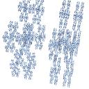
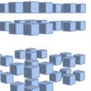
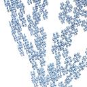
Class 2
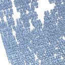
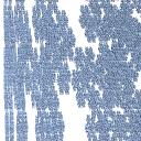
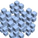
Class 3

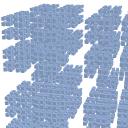
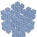
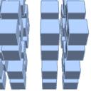
Figure 4.1. A random sample of the dataset of 3D Cantor images.

Model: "Cantor-activation"
Layer (type)	Output Shape	Param #
input_1 (InputLayer)	(None, 128, 128, 3)	0
rescaling (Rescaling)	(None, 128, 128, 3)	0
conv2d (Conv2D)	(None, 126, 126, 16)	448
max_pooling2d (MaxPooling2D)	(None, 63, 63, 16)	0
conv2d_1 (Conv2D)	(None, 61, 61, 32)	4640
max_pooling2d_1 (MaxPooling2D)	(None, 30, 30, 32)	0
conv2d_2 (Conv2D)	(None, 28, 28, 64)	18496
max_pooling2d_2 (MaxPooling2D)	(None, 14, 14, 64)	0
conv2d_3 (Conv2D)	(None, 12, 12, 128)	73856
flatten (Flatten)	(None, 18432)	0
dense (Dense)	(None, 3)	55299

Figure 4.2. A ConvNet for fractal image classification.

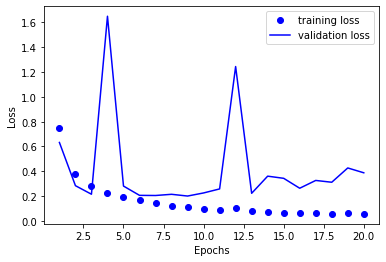
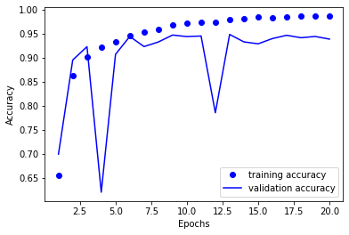
(a) Relu activation

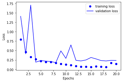
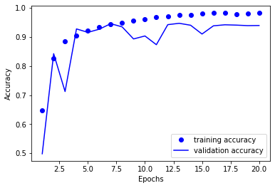
(b) Cantor-like activation

Figure 4.3. Training loss and validation loss, illustrated with use of a ConvNet.

References

- [AJ21] Daniel Alpay and Palle E. T. Jorgensen, New characterizations of reproducing kernel Hilbert spaces and applications to metric geometry, Opuscula Math. 41 (2021), no. 3, 283–300. MR 4302453
- [AJV14] Daniel Alpay, Palle Jorgensen, and Dan Volok, Relative reproducing kernel Hilbert spaces, Proc. Amer. Math. Soc. 142 (2014), no. 11, 3889–3895. MR 3251728
- [AK23] George A. Anastassiou and Seda Karateke, Richards’s curve induced Banach space valued ordinary and fractional neural network approximation, Rev. R. Acad. Cienc. Exactas Fís. Nat. Ser. A Mat. RACSAM 117 (2023), no. 1, Paper No. 14. MR 4505203
- [ASA+23] Mohd Rashid Admon, Norazak Senu, Ali Ahmadian, Zanariah Abdul Majid, and Soheil Salahshour, A new efficient algorithm based on feedforward neural network for solving differential equations of fractional order, Commun. Nonlinear Sci. Numer. Simul. 117 (2023), Paper No. 106968. MR 4512468
- [BSW23] S. Bickel, B. Schleich, and S. Wartzack, A Novel Shape Retrieval Method for 3D Mechanical Components Based on Object Projection, Pre-Trained Deep Learning Models and Autoencoder, Comput.-Aided Des. 154 (2023), Paper No. 103417. MR 4492099
- [CC21] Zhixiang Chen and Feilong Cao, Construction of feedforward neural networks with simple architectures and approximation abilities, Math. Methods Appl. Sci. 44 (2021), no. 2, 1788–1795. MR 4185345
- [CCK22] Lucian Coroianu, Danilo Costarelli, and Uğur Kadak, Quantitative estimates for neural network operators implied by the asymptotic behaviour of the sigmoidal activation functions, Mediterr. J. Math. 19 (2022), no. 5, Paper No. 211, 25. MR 4476907
- [CKM22] Sitan Chen, Adam R. Klivans, and Raghu Meka, Learning deep ReLU networks is fixed-parameter tractable, 2021 IEEE 62nd Annual Symposium on Foundations of Computer Science—FOCS 2021, IEEE Computer Soc., Los Alamitos, CA, [2022] ©2022, pp. 696–707. MR 4399726
- [CL22] Hengjie Chen and Zhong Li, A note on the applications of one primary function in deep neural networks, Int. J. Wavelets Multiresolut. Inf. Process. 20 (2022), no. 4, Paper No. 2150058, 18. MR 4458444
- [CST01] Nello Cristianini and John Shawe-Taylor, An introduction to support vector machines and other kernel-based learning methods., repr. ed., Cambridge: Cambridge University Press, 2001 (English).
- [DWZ+23] Zeyu Dong, Xin Wang, Xian Zhang, Mengjie Hu, and Thach Ngoc Dinh, Global exponential synchronization of discrete-time high-order switched neural networks and its application to multi-channel audio encryption, Nonlinear Anal. Hybrid Syst. 47 (2023), Paper No. 101291. MR 4491367
- [Eng96] Miroslav Engliš, Berezin quantization and reproducing kernels on complex domains, Trans. Amer. Math. Soc. 348 (1996), no. 2, 411–479. MR 1340173
- [GK23] Philipp Grohs and Gitta Kutyniok (eds.), Mathematical aspects of deep learning, Cambridge University Press, Cambridge, 2023. MR 4505882
- [GKNV22] Rémi Gribonval, Gitta Kutyniok, Morten Nielsen, and Felix Voigtlaender, Approximation spaces of deep neural networks, Constr. Approx. 55 (2022), no. 1, 259–367. MR 4376564
- [GKP20] Ingo Gühring, Gitta Kutyniok, and Philipp Petersen, Error bounds for approximations with deep ReLU neural networks in norms, Anal. Appl. (Singap.) 18 (2020), no. 5, 803–859. MR 4131039
- [GPR+21] Moritz Geist, Philipp Petersen, Mones Raslan, Reinhold Schneider, and Gitta Kutyniok, Numerical solution of the parametric diffusion equation by deep neural networks, J. Sci. Comput. 88 (2021), no. 1, Paper No. 22, 37. MR 4268857
- [Han16] Muhammad Hanif, Gauss-Newton method for feedforward artificial neural networks, Int. J. Math. Comput. 27 (2016), no. 3, 132–147. MR 3457582
- [HL23] Yuecai Han and Nan Li, A new deep neural network algorithm for multiple stopping with applications in options pricing, Commun. Nonlinear Sci. Numer. Simul. 117 (2023), Paper No. 106881. MR 4496811
- [HST10] David R. Hardoon and John Shawe-Taylor, Decomposing the tensor kernel support vector machine for neuroscience data with structured labels, Mach. Learn. 79 (2010), no. 1-2, 29–46. MR 3108145
- [HSTHD11] Zakria Hussain, John Shawe-Taylor, David R. Hardoon, and Charanpal Dhanjal, Design and generalization analysis of orthogonal matching pursuit algorithms, IEEE Trans. Inform. Theory 57 (2011), no. 8, 5326–5341. MR 2849119
- [JR22] Arnulf Jentzen and Adrian Riekert, A proof of convergence for stochastic gradient descent in the training of artificial neural networks with ReLU activation for constant target functions, Z. Angew. Math. Phys. 73 (2022), no. 5, Paper No. 188, 30. MR 4468133
- [JR23] by same author, Convergence analysis for gradient flows in the training of artificial neural networks with ReLU activation, J. Math. Anal. Appl. 517 (2023), no. 2, Paper No. 126601, 43. MR 4473797
- [JT18] Palle E.T. Jorgensen and Feng Tian, Duality for gaussian processes from random signed measures, ch. 2, pp. 23–56, John Wiley & Sons, Ltd, 2018.
- [JT20] Palle E. T. Jorgensen and Feng Tian, Spectral pairs and positive-definite-tempered distributions, Analysis, probability and mathematical physics on fractals, Fractals Dyn. Math. Sci. Arts Theory Appl., vol. 5, World Sci. Publ., Hackensack, NJ, [2020] ©2020, pp. 223–241. MR 4472250
- [JT21] Palle Jorgensen and James Tian, Infinite-dimensional analysis—operators in Hilbert space; stochastic calculus via representations, and duality theory, World Scientific Publishing Co. Pte. Ltd., Hackensack, NJ, [2021] ©2021. MR 4274591
- [JT22] by same author, Reproducing kernels and choices of associated feature spaces, in the form of -spaces, J. Math. Anal. Appl. 505 (2022), no. 2, Paper No. 125535, 31. MR 4295177
- [KG22] Wei Kang and Qi Gong, Feedforward neural networks and compositional functions with applications to dynamical systems, SIAM J. Control Optim. 60 (2022), no. 2, 786–813. MR 4395164
- [KLLW21] Shi-Lei Kong, Ka-Sing Lau, Jun Jason Luo, and Xiang-Yang Wang, Hyperbolic graphs induced by iterations and applications in fractals, Analysis and partial differential equations on manifolds, fractals and graphs, Adv. Anal. Geom., vol. 3, De Gruyter, Berlin, [2021] ©2021, pp. 143–181. MR 4320089
- [KLW20] Shi-Lei Kong, Ka-Sing Lau, and Ting-Kam Leonard Wong, Random walks and induced Dirichlet forms on compact spaces of homogeneous type, Analysis, probability and mathematical physics on fractals, Fractals Dyn. Math. Sci. Arts Theory Appl., vol. 5, World Sci. Publ., Hackensack, NJ, [2020] ©2020, pp. 273–296. MR 4472252
- [Kut20] Gitta Kutyniok, Discussion of: “Nonparametric regression using deep neural networks with ReLU activation function” [ MR4134774], Ann. Statist. 48 (2020), no. 4, 1902–1905. MR 4134776
- [MCA20] Adrian Moldovan, Angel Caţaron, and Răzvan Andonie, Learning in feedforward neural networks accelerated by transfer entropy, Entropy 22 (2020), no. 1, Paper No. 102, 19. MR 4072078
- [MK23] Krzysztof Martyn and Mił osz Kadziński, Deep preference learning for multiple criteria decision analysis, European J. Oper. Res. 305 (2023), no. 2, 781–805. MR 4503771
- [MM23] Thomas Merkh and Guido Montúfar, Stochastic feedforward neural networks: universal approximation, Mathematical aspects of deep learning, Cambridge Univ. Press, Cambridge, 2023, pp. 267–314. MR 4505888
- [OSZ22] Joost A. A. Opschoor, Christoph Schwab, and Jakob Zech, Deep learning in high dimension: ReLU neural network expression for Bayesian PDE inversion, Optimization and control for partial differential equations—uncertainty quantification, open and closed-loop control, and shape optimization, Radon Ser. Comput. Appl. Math., vol. 29, De Gruyter, Berlin, [2022] ©2022, pp. 419–462. MR 4409717
- [PORSTS21] María Pérez-Ortiz, Omar Rivasplata, John Shawe-Taylor, and Csaba Szepesvári, Tighter risk certificates for neural networks, J. Mach. Learn. Res. 22 (2021), Paper No. 227, 40. MR 4329806
- [RSSST06] Juho Rousu, Craig Saunders, Sandor Szedmak, and John Shawe-Taylor, Kernel-based learning of hierarchical multilabel classification models, J. Mach. Learn. Res. 7 (2006), 1601–1626. MR 2274418
- [SHO22] Alexandre Smirnov, Boumediene Hamzi, and Houman Owhadi, Mean-field limits of trained weights in deep learning: a dynamical systems perspective, Dolomites Res. Notes Approx. 15 (2022), no. Special Issue dedicated to Robert Schaback on the occasion of his 75th birthday, 125–145. MR 4500409
- [STWCK05] John Shawe-Taylor, Christopher K. I. Williams, Nello Cristianini, and Jaz Kandola, On the eigenspectrum of the Gram matrix and the generalization error of kernel-PCA, IEEE Trans. Inform. Theory 51 (2005), no. 7, 2510–2522. MR 2246374
- [Sza83] F. H. Szafraniec, Interpolation and domination by positive definite kernels, Przestrzenie Hilberta z Jadrem Reprodukujacym (Reproducing Kernel Hilbert Spaces), Wydawnictwo Uniwersytetu Jagiellonskiego, Krakow,2004 (in Polish)., Lecture Notes in Math., vol. 1014, Springer, Berlin, 1983, pp. 291–295. MR 738131
- [Sza04] by same author, Przestrzenie Hilberta z Jadrem Reprodukujacym (in Polish), Wydawnictwo Uniwersytetu Jagiellonskiego, Krakow, 2004.
- [Sza15a] Franciszek Hugon Szafraniec, The reproducing kernel property and its space: more or less standard examples of applications, Operator theory. With 51 figures and 2 tables. In 2 volumes, Basel: Springer, 2015, pp. 31–58 (English).
- [Sza15b] by same author, The reproducing kernel property and its space: the basics, Operator theory. With 51 figures and 2 tables. In 2 volumes, Basel: Springer, 2015, pp. 3–30 (English).
- [Sza21] by same author, Revitalising Pedrick’s approach to reproducing kernel Hilbert spaces, Complex Anal. Oper. Theory 15 (2021), no. 4, Paper No. 66, 12. MR 4250453
- [ZC23] Guodong Zhang and Jinde Cao, New results on fixed/predefined-time synchronization of delayed fuzzy inertial discontinuous neural networks: Non-reduced order approach, Appl. Math. Comput. 440 (2023), Paper No. 127671. MR 4505410