The dipole cross section by the unintegrated gluon distribution at small $x$

Abstract

We apply a previously developed scheme to consistently include the improved saturation model for the unintegrated gluon distribution (UGD) in order to evaluate, in the framework of $k_{t}$ factorization, at small $x$ at the next-to-leading order (NLO) in $\alpha_{s}$. We start the unintegrated gluon distribution with a parametrization of the deep inelastic structure function for electromagnetic scattering with protons, and then extract the color dipole cross section, which preserves its behavior success in a wide range of $k_{t}^{2}$ in comparisons with the UGD models (M. Hentschinski, A. Sabio Vera and C. Salas (HSS), I.P.Ivanov and N.N.Nikolaev (IN) and G. Watt, A.D. Martin and M.G. Ryskin (WMR)) . These results show that the geometric scaling holds for the improved saturation model in a wide kinematic region $rQ_{s}$, and are comparable with the Golec-Biernat-W$\ddot{\mathrm{u}}$sthoff (GBW) model. The unintegrated gluon distribution at low and high momentum transfer in a wide range of $x$ is considered.

.1 I. Introduction

Although our knowledge of the proton structure at small-$x$ is very limited, novel opportunities will be opened at new-generation facilities (Electron-Ion Collider(EIC), High-Luminosity Large Hadron Collider (HL-LHC), Forward Physics Facility (FPF)). Combining the information coming from dipole cross sections and $p_{T}$-unintegrated densities could play an important role. In particular, polarized amplitudes and cross sections for the exclusive electroproduction of $\rho$ and $\phi$ mesons at the Hadron-Electron Ring Accelerator (HERA) and the EIC are very sensitive to the unintegrated gluon distribution (UGD) model adopted, whereas forward Drell-Yan dilepton distributions at the Large Hadron Collider beauty (LHCb) are very sensitive to next-to-leading logarithmic corrections. Indeed, the dipole cross section is directly connected via a Fourier transform to the small-x UGD, whose evolution in $x$ is regulated by the Balitsky- Fadin-Kuraev-Lipatov (BFKL) equation [1]. The BFKL equation retains the full $Q^{2}$ dependence and not just the leading $\ln{Q^{2}}$ terms. Indeed the resummation of terms is proportional to $\alpha_{s}\ln(1/x)$ to all orders. This involves considering this means that we do not have strongly ordered $k_{t}$ but instead integrate over the full range of $k_{t}$ in phase space of the gluons [2,3]. The BFKL equation governs the evolution of the UGD, where the $k_{t}$-factorization is used in the high energy limit in which the QCD interaction is described in terms of the quantity which depends on the transverse momentum of the gluon [4]. In the $k_{t}$-factorization framework, the gluon distribution depends on $x$ and $k_{t}^{2}$, where $x$ and $k^{2}_{t}$ being the fractional momentum of proton carried by gluon and the transverse momentum of gluon respectively. At high energies, the $k_{t}$-factorization is a suitable formalism to compute the relevant distribution and cross sections. Within this regime, the longitudinal momentum fraction of partons, $x$, is small. The unintegrated gluon distribution function is thus of great phenomenological and theoretical interest to develop the formalism which includes the transverse momentum dependence in the context of the multigluon distributions.
It is more appropriate to use the parton distributions unintegrated over the transverse momentum $k_{t}$ in the framework of $k_{t}$-factorization QCD approach for semi-inclusive processes (such as inclusive jet production in DIS, electroweak boson production, etc.) at high energies. The $k_{t}$-factorization formalism provides solid theoretical grounds for the effects of initial gluon radiation and intrinsic parton transverse momentum $k_{t}$. The unintegrated gluon $f(x,k_{t}^{2})$ distribution is directly related to the dipole-nucleon cross section, that is saturated at low $Q$ or large transverse distances $r{\sim}1/Q$ between quark $q$ and antiquark $\overline{q}$ in the $q\overline{q}$ dipole created from the splitting of the virtual photon $\gamma^{*}$ in the ep DIS. Indeed, the suitable factorization approach in DIS (where $W{\gg}Q{\gg}\Lambda_{\mathrm{QCD}}$) is provided by $k_{t}$-factorization [5].
The UGD, in its original definition, obeys the BFKL evolution equation in the $x$ variable and being a nonperturbative quantity. To realistically describe the structure of the proton, we must introduce a $k_{t}$ unintegrated gluon density, whose evolution at small-$x$ is governed by the BFKL equation [6]. The object of the BFKL evolution equation at very small $x$ is the differential gluon structure function of proton

$$f(x,k_{t}^{2}) = \frac{\partial{xg(x,\mu^{2})}}{\partial{\ln}\mu^{2}}|_{\mu^{2}=k^{2}_{t}}$$ (1)

which emerges in the color dipole picture (CDP) of inclusive deep inelastic scattering (DIS) and diffractive DIS into dijets [7]. Unintegrated distributions are required to describe measurements where transverse momenta are exposed explicitly.
The unintegrated gluon distribution function satisfies the BFKL equation for an alternative derivation in terms of color dipoles. The BFKL equation at leading order is given by

$$\frac{{\partial}f(x,k^{2}_{t})}{{\partial}{\ln}({1}/{x})}=\int{dk^{\prime 2}_{t}}K(k^{2}_{t},k^{\prime 2}_{t})f(x,k^{\prime 2}_{t}),$$ (2)

which describes the evolution in ${\ln}({1}/{x})$ of the unintegrated gluon density and $K$ is the BFKL kernel [2,3]. In the small $x$ limit this basically gives a power law behavior in $x$,

$$f(x,k^{2}_{t}){\sim}h(k^{2}_{t})x^{-\lambda},$$ (3)

where $h{\sim}(k^{2}_{t})^{-\frac{1}{2}}$ at large $k^{2}_{t}$ and $\lambda$ is the maximum eigenvalue of the kernel $K$ of the BFKL equation. For fixed $\alpha_{s}$, $\lambda$ has the value $\lambda=\frac{\alpha_{s}}{\pi}12\ln 2$, where this hard Pomeron has been termed the BFKL Pomeron and lead to very steeply rising $V^{*}N$ cross-sections. In the BFKL analysis, there are infra-red (IR) and ultra-violet (UV) cutoffs on the $k^{2}_{t}$ integrations. Indeed determining the IR cutoff parameter is important for the integrating ${\int}dk^{2}_{t}\alpha_{s}(k^{2}_{t})$ down to $k^{2}_{t}=0$, also the choice of the UV cutoff is important when working at finite order [8,9].
The color dipole picture (CDP) [10] has been introduced to study a wide variety of small $x$ inclusive and diffractive processes at HERA. The CDP, at small $x$, gives a clear interpretation of the high-energy interactions, where is characterized by high gluon densities because the proton structure is dominated by dense gluon systems [11-13] and predicts that the small $x$ gluons in a hadron wavefunction should form a Color Glass Condensate [14]. Dipole representation provides a convenient description of DIS at small $x$. There, the scattering between the virtual photon $\gamma^{*}$ and the proton is seen as the color dipole where the transverse dipole size $r$ and the longitudinal momentum fraction $z$ with respect to the photon momentum are defined. The amplitude for the complete process is simply the production of these subprocess amplitudes, as the DIS cross section is factorized into a light-cone wave function and a dipole cross section. Using the optical theorem, this leads to the following expression for the $\gamma^{*}p$ cross-sections

$$\sigma_{L,T}^{\gamma^{*}p}(x,Q^{2})=\int dzd^{2}\mathbf{r}|\Psi_{L,T}(\mathbf{r},z,Q^{2})|^{2}\sigma_{\mathrm{dip}}({x},\mathbf{r}),$$ (4)

where subscripts $L$ and $T$ referring to the transverse and longitudinal polarization state of the exchanged boson. Here $\Psi_{L,T}$ are the appropriate spin averaged light-cone wave functions of the photon and $\sigma_{\mathrm{dip}}({x},r)$ is the dipole cross-section which related to the imaginary part of the $(q\overline{q})p$ forward scattering amplitude. The variable $z$, with $0\leq z\leq 1$, characterizes the distribution of the momenta between quark and antiquark. The square of the photon wave function describes the probability for the occurrence of a $(q\overline{q})$ fluctuation of transverse size with respect to the photon polarization.
Another framework which can be used for calculating the parton distributions is based on the Dokshitzer-Gribov-Lipatov-Altarelli-Parisi (DGLAP) evolution equations [15]. Deep inelastic electron-proton scattering is described in terms of scale dependent parton densities $q(x,\mu^{2})$ and $g(x,\mu^{2})$ [16], where the integrated gluon distribution ($xg(x,\mu^{2})$) is defined through the unintegrated gluon distribution ($f(x,k_{t}^{2})$) by

$$xg(x,\mu^{2}) {\equiv} \int^{\mu^{2}}\frac{dk_{t}^{2}}{k_{t}^{2}}f(x,k_{t}^{2}).$$ (5)

The unintegrated gluon distribution is related to the dipole cross section [4, 17]

$$\sigma(x,\mathbf{r})=\frac{8\pi^{2}}{N_{c}}\int\frac{dk_{t}}{k_{t}^{{}^{3}}}[1-J_{0}(k_{t}\mathbf{r})]\alpha_{s}f(x,k_{t}^{2}).$$ (6)

A novel formulation of the UGD for DIS in a way that accounts for the leading powers in both the Regge and Bjorken limits is presented in Ref.[18]. In this way, the UGD is defined by an explicit dependence on the longitudinal momentum fraction $x$ which entirely spans both the dipole operator and the gluonic Parton Distribution Function (PDF).
In addition to the gluon momentum derivative model (i.e., Eq.(1)), several other models [7,10, 19-21] for the UGD have also been proposed so far. A comparison between these models can be found in Refs.[22,23]. The authors in Ref. [19] presented an $x$-independent model (ABIPSW) of the UGD where merely coincides with the proton impact factor by the following form

$$f(x,k_{t}^{2})=\frac{A}{4\pi^{2}M^{2}}\Big{[}\frac{k_{t}^{2}}{M^{2}+k_{t}^{2}}\Big{]},$$ (7)

where M is a characteristic soft scale and A is the normalisation factor.
The authors in Ref. [7] presented a UGD soft-hard model (IN) in the large and small $k_{t}$ regions by the following form

$$f(x,k_{t}^{2})=f_{\mathrm{soft}}^{(B)}(x,k_{t}^{2})\frac{k_{s}^{2}}{k_{s}^{2}+k_{t}^{2}}+f_{\mathrm{\mathrm{hard}}}(x,k_{t}^{2})\frac{k_{t}^{2}}{k_{h}^{2}+k_{t}^{2}},$$ (8)

where the soft and the hard components are defined in [7].
The UGD model was considered in [20] to used in the study of DIS structure functions and takes the form of a convolution between the BFKL gluon Green^,s function and a leading-order (LO) proton impact factor, where has been employed in the description of single-bottom quark production at LHC and to investigate the photoproduction of $J/\Psi$ and $\Upsilon$, by the following form (HSS model)

$$f(x,k_{t}^{2},M_{{h}}) = \int_{-\infty}^{+\infty}\frac{d\nu}{2\pi^{2}}\mathcal{C}\frac{\Gamma(\delta-i\nu-\frac{1}{2})}{\Gamma(\delta)}(\frac{1}{x})^{\chi(\frac{1}{2}+i\nu)}(\frac{k_{t}^{2}}{Q_{0}^{2}})^{\frac{1}{2}+i\nu}\Bigg{\{}1+\frac{\overline{\alpha}_{s}^{2}\beta_{0}\chi_{0}(\frac{1}{2}+i\nu)}{8N_{c}}\log(\frac{1}{x})$$ (9)

$${\times}\Bigg{[}-\psi(\frac{1}{2}+i\nu)-\log\frac{k_{t}^{2}}{M^{2}_{{h}}}\Bigg{\}}\Bigg{]},$$

where $\chi_{0}(\frac{1}{2}+i\nu)$ and $\chi(\gamma)$ are respectively the LO and the next-to-leading order (NLO) eigenvalues of the BFKL kernel and $\beta_{0}=11-\frac{2}{3}n_{f}$ with $n_{f}$ the number of active quarks. The LO eigenvalue of the BFKL kernel is $\chi_{0}(\frac{1}{2}+i\nu){\equiv}\chi_{0}(\gamma)=2\psi(1)-\psi(\gamma)-\psi(1-\gamma)$ and the NLO eigenvalue of the BFKL kernel is $\chi(\gamma)=\overline{\alpha_{s}}\chi_{0}(\gamma)+\overline{\alpha_{s}}^{2}\chi_{1}(\gamma)-\frac{1}{2}\overline{\alpha_{s}}^{2}\chi^{\prime}_{0}(\gamma)\chi_{0}(\gamma)+\chi_{RG}(\overline{\alpha_{s}},\gamma)$ with $\psi(\gamma)$ is the logarithmic derivative of the Euler Gamma function. Here $\overline{\alpha}_{s}=\frac{3}{\pi}\alpha_{s}(\mu^{2})$ with $\mu^{2}=Q_{0}M_{h}$ where $M_{h}$ plays the role of the hard scale which can be identified with the photon virtuality, $\sqrt{Q^{2}}$.
The authors in Ref. [21] presented a UGD model (Watt-Martin-Ryskin (WMR) model) where depends on an extra-scale $\mu$, fixed at $Q$, by the following form

$$f(x,k_{t}^{2},\mu^{2}) = T_{g}(k_{t}^{2},\mu^{2})\frac{\alpha_{s}(k_{t}^{2})}{2\pi}\int_{x}^{1}dz\Bigg{[}\sum_{q}P_{gq}(z)\frac{x}{z}q(\frac{x}{z},k_{t}^{2})+P_{gg}(z)\frac{x}{z}g(\frac{x}{z},k_{t}^{2})\Theta(\frac{\mu}{\mu+k_{t}}-z)\Bigg{]},$$ (10)

where $T_{g}(k_{t}^{2},\mu^{2})$ gives the probability of evolving from the scale $k_{t}$ to the scale $\mu$ without parton emission and $P_{ij}^{,}$s are the splitting functions.
Golec-Biernat-Wusthoff (GBW) [10] presented a UGD model where derives from the effective dipole cross section $\sigma(x,\mathbf{r})$ for the scattering of a $q\overline{q}$ pair of a nucleon as

$$f(x,k_{t}^{2}) = k_{t}^{4}\sigma_{0}\frac{R_{0}^{2}(x)}{2\pi}e^{-k_{t}^{2}R_{0}^{2}(x)},$$ (11)

with $R_{0}^{2}(x)=\frac{1}{\mathrm{GeV}^{2}}(\frac{x}{x_{0}})^{\lambda_{p}}$ and the following values $\sigma_{0}=23.03~{}\mathrm{mb}$, $\lambda_{p}=0.288$ and $x_{0}=3.04{\times}10^{-4}$. Although one of them (the HSS one) was fitted to reproduce DIS structure functions, the study of other reactions has provided an evidence that the UGD is not yet well known. The HSS model also reproduces well the forward Drell-Yan data at the LHC without any further adjustment of extra parameters [24]. In this paper we use the DGLAP-improved saturation model with respect to the UGD in the proton to access the dipole cross section at low $x$.

.2 II. Method

The interaction of the $q\overline{q}$ pair with the proton is described by the dipole cross section. It is related to the gluon density in the target by the $k_{T}$-factorization formula [7,10,17]

$$\sigma(x,r)=\int\frac{d^{2}k_{t}}{k_{t}^{{}^{4}}}\frac{\partial{xg(x,k^{2}_{t})}}{\partial{\ln}k^{2}_{t}}[1-e^{i\mathbf{k}_{t}.\mathbf{r}}][1-e^{-i\mathbf{k}_{t}.\mathbf{r}}],$$ (12)

where the relation between $f(x,k^{2}_{t})$ and $xg(x,k^{2}_{t})$ defined through Eq.(1). In the following we present a method of extraction of the gluon distribution function in the kinematic region of low values of the Bjorken variable $x$ from the structure $F_{2}(x,k^{2}_{t})$ and derivative $\partial{F_{2}(x,k^{2}_{t})}/\partial{\ln}k^{2}_{t}$ by relying on the DGLAP $Q^{2}$-evolution equations. The structure function $F_{2}$ is expressed via the singlet and gluon distributions as

$$F_{2}(x,k^{2}_{t})=<e^{2}>\bigg{[}B_{2,s}(x){\otimes}xf_{s}(x,k^{2}_{t})+B_{2,g}(x){\otimes}xg(x,k^{2}_{t})\bigg{]},$$ (13)

where $<e^{2}>$ is the average of the charge $e^{2}$ for the active quark flavors $n_{f}$ , $<e^{2}>=n_{f}^{-1}\sum_{i=1}^{n_{f}}e_{i}^{2}$ and the nonsinglet densities become negligibly small in comparison with the singlet densities at small $x$. The quantities $B_{2,i}(x)(i=s,g)$ are the known Wilson coefficient functions and the symbol $\otimes$ denotes convolution according to the usual prescription. According to the DGLAP evolution equations, the singlet distribution function leads to the following relation of integro-differential equation [25]

$$\frac{{\partial}F_{2}(x,k^{2}_{t})}{{\partial}{\ln}k^{2}_{t}} = -\frac{a_{s}(k^{2}_{t})}{2}[P_{qq}(x){\otimes}F_{2}(x,k^{2}_{t})+<e^{2}>P_{qg}(x){\otimes}xg(x,k^{2}_{t})],$$ (14)

where

$$P_{a,b}(x)=P_{a,b}^{(0)}(x)+a_{s}(k^{2}_{t})\widetilde{P}_{a,b}^{(1)}(x)+a_{s}^{2}(k^{2}_{t})\widetilde{P}_{a,b}^{(2)}(x)$$ (15)

and

$$\widetilde{P}_{ab}^{(n)}(x)={P}_{ab}^{(n)}(x)+[C_{2,s}+C_{2,g}+...]\otimes{P}_{ab}^{(0)}(x)+....$$

The quantities $\widetilde{P}_{ab}$${}^{,}s$ are expressed via the known splitting and Wilson coefficient functions in literatures [26,27] and $a_{s}(k^{2}_{t})=\alpha_{s}(k^{2}_{t})/4\pi$.
Considering the variable definitions $\upsilon{\equiv}\ln(1/x)$ and $w{\equiv}\ln(1/z)$, one can rewrite Eq.(14) in terms of the convolution integrals and new variables as

$$\frac{\partial{\mathcal{\widehat{F}}_{2}(\upsilon,k^{2}_{t})}}{\partial{\ln}k^{2}_{t}} = \int_{0}^{\upsilon}[\mathcal{\widehat{F}}_{2}(\upsilon,k^{2}_{t})\mathcal{\widehat{H}}^{(\varphi)}_{2,s}(a_{s}(k^{2}_{t}),\upsilon-w)+<e^{2}>\mathcal{\widehat{G}}(\upsilon,k^{2}_{t})\mathcal{\widehat{H}}^{(\varphi)}_{2,g}(a_{s}(k^{2}_{t}),\upsilon-w)]dw,$$ (16)

where

$$\frac{\partial{\mathcal{\widehat{F}}_{2}(\upsilon,k^{2}_{t})}}{\partial{\ln}k^{2}_{t}}{\equiv}\frac{{\partial}F_{2}(e^{-\upsilon},k^{2}_{t})}{\partial{\ln}k^{2}_{t}},~{}\mathcal{\widehat{G}}(\upsilon,k^{2}_{t}){\equiv}xg(e^{-\upsilon},k^{2}_{t}),~{}\mathcal{\widehat{H}}^{(\varphi)}(a_{s}(k^{2}_{t}),\upsilon){\equiv}e^{-\upsilon}\widehat{P}_{a,b}^{(\varphi)}(a_{s}(k^{2}_{t}),\upsilon).$$ (17)

The splitting function reads

$$P_{a,b}^{(\varphi)}(a_{s},x)=\sum_{n=0}^{\varphi}a_{s}^{n+1}(k^{2}_{t})P_{a,b}^{(n)}(x),$$ (18)

where $n$ denotes the order in running coupling $\alpha_{s}(k^{2}_{t})$. The Laplace transform of $\mathcal{\widehat{H}}(a_{s}(k^{2}_{t}),\upsilon)$${}^{,}s$ are given by the following forms

$$\Phi_{f}^{(\varphi)}(a_{s}(k^{2}_{t}),s) {\equiv} {\mathcal{L}}[\mathcal{\widehat{H}}^{(\varphi)}_{2,s}(a_{s}(k^{2}_{t}),\upsilon);s]=\int_{0}^{\infty}\mathcal{\widehat{H}}^{(\varphi)}_{2,s}(a_{s}(k^{2}_{t}),\upsilon)e^{-s\upsilon}d\upsilon,$$

$$\Theta_{f}^{(\varphi)}(a_{s}(k^{2}_{t}),s) {\equiv} {\mathcal{L}}[\mathcal{\widehat{H}}^{(\varphi)}_{2,g}(a_{s}(k^{2}_{t}),\upsilon);s]=\int_{0}^{\infty}\mathcal{\widehat{H}}^{(\varphi)}_{2,g}(a_{s}(k^{2}_{t}),\upsilon)e^{-s\upsilon}d\upsilon.$$ (19)

We know that the Laplace transforms of the convolution factors are simply the ordinary products of the Laplace transforms of the factors. Therefore, Eq.(16) in the Laplace space $s$ reads as

$$\frac{\partial{f_{2}(s,k^{2}_{t})}}{\partial{\ln}k^{2}_{t}} = \Phi_{f}^{(\varphi)}(a_{s}(k^{2}_{t}),s)f_{2}(s,k^{2}_{t})+<e^{2}>\Theta_{f}^{(\varphi)}(a_{s}(k^{2}_{t}),s)xg(s,k^{2}_{t}),$$ (20)

where

$${\mathcal{L}}[\mathcal{\widehat{F}}_{2}(\upsilon,k^{2}_{t});s]=f_{2}(s,k^{2}_{t}),~{}{\mathcal{L}}[\mathcal{\widehat{G}}(\upsilon,k^{2}_{t});s]=xg(s,k^{2}_{t}).$$ (21)

The gluon distribution into the parametrization of the proton structure function and its derivative with respect to ${\ln}k^{2}_{t}$ in $s$-space in Eq.(20) is given by the following form

$$xg(s,k^{2}_{t}) = k^{(\varphi)}(a_{s}(k^{2}_{t}),s)Df_{2}(s,k^{2}_{t})-h^{(\varphi)}(a_{s}(k^{2}_{t}),s)f_{2}(s,k^{2}_{t}),$$ (22)

where

$$Df_{2}(s,k^{2}_{t}) = {\partial{f_{2}(s,k^{2}_{t})}}/{\partial{\ln}k^{2}_{t}},$$

$$k^{(\varphi)}(a_{s}(k^{2}_{t}),s) = 1/(<e^{2}>\Theta^{(\varphi)}_{f}(a_{s}(k^{2}_{t}),s)),$$

$$h^{(\varphi)}(a_{s}(k^{2}_{t}),s) = \Phi^{(\varphi)}_{f}(a_{s}(k^{2}_{t}),s)k^{(\varphi)}(a_{s}(k^{2}_{t}),s).$$

The inverse Laplace transforms of Eq.(22) reads

$$\widehat{xg}^{(\varphi)}(\upsilon,k^{2}_{t}){\equiv}{\mathcal{L}}^{-1}[xg(s,k^{2}_{t});\upsilon]={\mathcal{L}}^{-1}[k^{(\varphi)}(a_{s}(k^{2}_{t}),s)Df_{2}(s,k^{2}_{t})-h^{(\varphi)}(a_{s}(k^{2}_{t}),s)f_{2}(s,k^{2}_{t});\upsilon]$$ (23)

where the inverse transform of a product to the convolution of the original functions, giving

$${\mathcal{L}}^{-1}[f(s){\times}h(s);\upsilon] = \int_{0}^{\upsilon}\widehat{F}(w)\widehat{H}(\upsilon-w)dw.$$

The inverse Laplace transform of the functions $k$ and $h$ in Eq.(23) are defined by ${\widehat{J}}(\upsilon)$ and ${\widehat{M}}(\upsilon)$, as

$$\widehat{J}(\upsilon,k^{2}_{t}){\equiv}{\mathcal{L}}^{-1}[k(s,k^{2}_{t});\upsilon],~{}\widehat{M}(\upsilon,k^{2}_{t}){\equiv}{\mathcal{L}}^{-1}[h(s,k^{2}_{t});\upsilon].$$ (24)

The functions $k$ and $h$ in $s$-space, into the Laplace transform of the splitting functions ($P_{qq}$ and $P_{qg}$), are given by [29]

$$k^{(n)}(a_{s}(k^{2}_{t}),s) = \bigg{(}<e^{2}>{\mathcal{L}}[e^{-\upsilon}\sum_{n=0}^{1}a_{s}^{n+1}(k^{2}_{t})\widehat{P}_{qg}^{(n)}(\upsilon);s]\bigg{)}^{-1},$$

$$h^{(n)}(a_{s}(k^{2}_{t},s) = \frac{{\mathcal{L}}[e^{-\upsilon}\sum_{n=0}^{1}a_{s}^{n+1}(k^{2}_{t})\widehat{P}_{qq}^{(n)}(\upsilon);s]}{<e^{2}>{\mathcal{L}}[e^{-\upsilon}\sum_{n=0}^{1}a_{s}^{n+1}(k^{2}_{t})\widehat{P}_{qg}^{(n)}(\upsilon);s]},$$ (25)

where at small $x$, the kernels at NLO approximation in Eq.(19) are given by the following forms

$$\Theta_{f}(a_{s},s) {\simeq} 2n_{f}a_{s}{\Big{[}}\frac{1}{1+s}-\frac{2}{2+s}+\frac{2}{3+s}{\Big{]}}+a^{2}_{s}C_{A}T_{f}{\Big{[}}\frac{40}{9s}{\Big{]}},$$

$$\Phi_{f}(a_{s},s) {\simeq} a_{s}{\Big{[}}4-\frac{8}{3}(\frac{1}{1+s}+\frac{1}{2+s}+2S_{1}(s){\Big{]}}+a^{2}_{s}C_{F}T_{f}{\Big{[}}\frac{40}{9s}{\Big{]}},$$ (26)

where $S_{1}(s)=\psi(s+1)+\gamma_{E}$, where $\psi(x)$ is the digamma function and $\gamma_{E}=0.5772156...$ is Euler constant. Here $C_{A}=N_{c}=3$, $C_{F}=\frac{N_{c}^{2}-1}{2N_{c}}=\frac{4}{3}$ and $T_{f}=\frac{1}{2}n_{f}$. The standard representation for QCD couplings in NLO (within the $\mathrm{\overline{MS}}$-scheme) approximation reads

$$\alpha^{\mathrm{NLO}}_{s}(k^{2}_{t}) = \frac{4\pi}{\beta_{0}\ln\frac{k^{2}_{t}}{\Lambda^{2}}}\Big{[}1-\frac{\beta_{1}}{\beta_{0}^{2}}\frac{\ln{\ln\frac{k^{2}_{t}}{\Lambda^{2}}}}{\ln\frac{k^{2}_{t}}{\Lambda^{2}}}\Big{]},$$ (27)

where $\beta_{0}$ and $\beta_{1}$ are the one and two loop correction to the QCD $\beta$-function and $\Lambda$ is the QCD cut-off parameter.
Therefore, the integrated gluon density is related to the proton structure function by the following form

$$xg^{(\varphi)}(x,k^{2}_{t}) = \int_{x}^{1}\Big{[}{DF}_{2}(\ln\frac{1}{y},k^{2}_{t}){J}(a_{s}(k^{2}_{t}),\ln\frac{y}{x})-{F}_{2}(\ln\frac{1}{y},k^{2}_{t}){M}(a_{s}(k^{2}_{t}),\ln\frac{y}{x})\Big{]}\frac{dy}{y},$$ (28)

where $F_{2}(x,k^{2}_{t})$ is the proton structure function. The parametrization of $F_{2}$ in Ref.[30] has an expression for the asymptotic part of $F_{2}$ (no-valence) that accounts for the asymptotic behavior $F_{2}{\simeq}\ln^{2}(1/x)$ at small $x$ which describes fairly well the available experimental data on the reduced cross sections.
In next section we consider the UGD and the color dipole cross section due to the parametrization of the proton structure function in Eqs.(1) and (12) with respect to (28), respectively.

.3 3. Numerical Results

The UGD is obtained directly in terms of the parameterization of the structure function $F_{2}(x,k^{2}_{t})$ and its derivative. The resulting UGD with the $k^{2}_{t}$-dependence due to the parametrization of the proton structure function are shown in Fig. 1. In this figure, we plot the $k^{2}_{t}$ dependence of the UGD at $x=10^{-3}$ and compared the unintegrated gluon distribution behavior due to the improved saturation model with the GBW model. An enhancement and then depletion is observable in the improved and GBW models. These picks occur at $k^{2}_{t}{\approx}10~{}\mathrm{GeV}^{2}$ and $k^{2}_{t}{\approx}1~{}\mathrm{GeV}^{2}$ in the improved and GBW models respectively. As we can seen, the UGD behavior in the improved saturation model, in a wide range of $k^{2}_{t}$, is softer than the GBW model. The error bands in Fig.1 in the improved saturation model are due to the uncertainties in the coefficients of the parametrization of the proton structure function. The uncertainties are very small for low $k_{t}^{2}$ and increases as $k_{t}^{2}$ increase to $100~{}\mathrm{GeV}^{2}$.

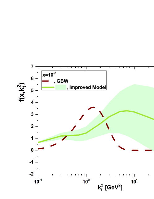
Figure 1: The UGD as a function of $k_{t}^{2}$ with respect to the improved model compared with the GBW model at $x=10^{-3}$. The error bands in the improved model are due to the statistical uncertainties in the coefficients of the parametrization $F_{2}$ in [30].

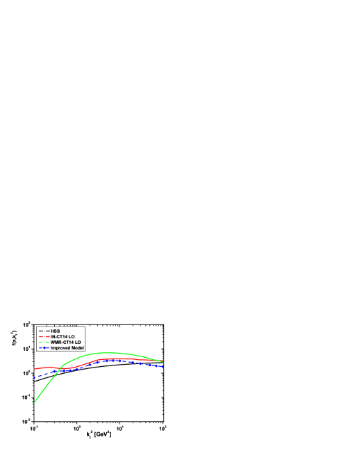
Figure 2: The unintegrated gluon distribution $f(x,k^{2}_{t})$ obtained from the improved saturation model (dashed-symbol), as a function of $k^{2}_{t}$ at $x=10^{-3}$, compared with the HSS [20], IN [7] and WMR [21] models.

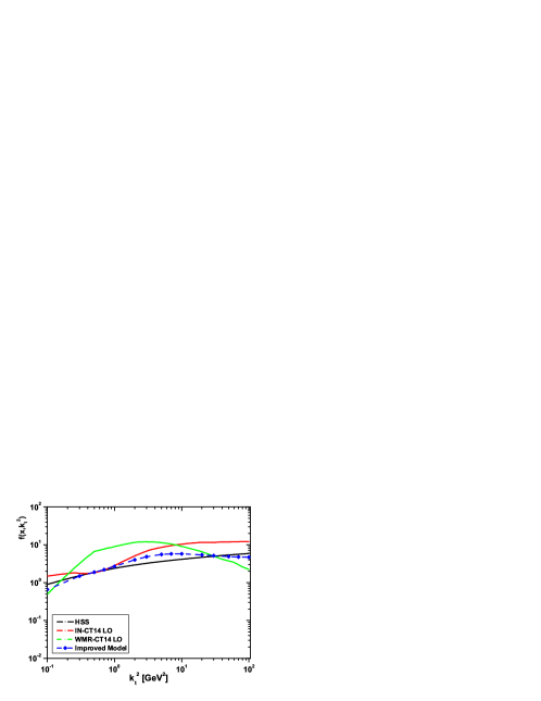
Figure 3: The same as Fig.2 for $x=10^{-4}$.

In Fig. 2 we show the $k_{t}$ distributions of three different unintegrated gluons at $x=10^{-3}$. This figure compares the results of the improved saturation model, based on the parametrization of the proton structure function, with the HSS [20], IN [7] and WMR [21] models. We observe that the improved saturation result is comparable with the HSS and IN models in a wide range of $k^{2}_{t}$. The differences are not large, however there is some suppression due to the models at large and small values of $k^{2}_{t}$. The continuous behavior of the UGD in our model with increases of $k^{2}_{t}$ is due to the gluon and quark terms included in the improved saturation model.

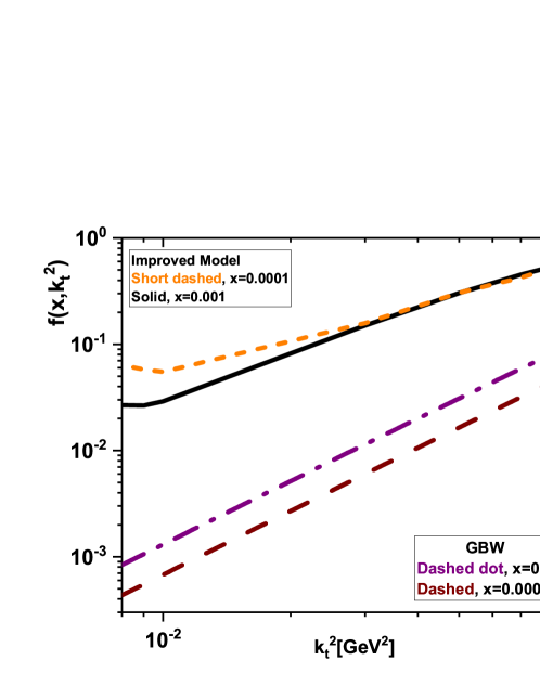
Figure 4: Low $k^{2}_{t}$-behavior of the considered UGD model for $x=10^{-3}$ and $10^{-4}$ (solid and short dashed curves) compared with the GBW model (dashed-dot and dashed curves) [10], respectively.

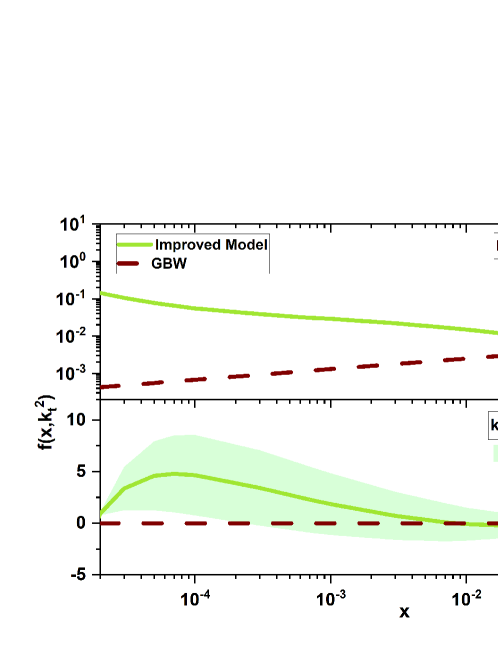
Figure 5: $x$-behavior of the considered UGD model (solid curves) for $k^{2}_{t}=0.01~{}\mathrm{GeV}^{2}$ (up) and $k^{2}_{t}=100~{}\mathrm{GeV}^{2}$ (down), as accompanied with the statistical uncertainties from the coefficients of the parameterization of $F_{2}$ in [30], compared with the GBW model (dashed curves) [10].

In Fig.3 we present the unintegrated gluons with the $k_{t}^{2}$-dependence of all the considered UGD models in Fig.2, for $x=10^{-4}$. The plot clearly shows the same behavior in the $k_{t}^{2}$-shape of the figures at low values of $x$. In conclusion, the consistency of the several UGDs in their $k_{t}$ dependence holds for values of $x=10^{-3}$ and $10^{-4}$ in a wide range of $k_{t}$. Calculation of the dipole cross section requires the knowledge of the unintegrated gluon density for all scales $0<k_{t}^{2}<\infty$. Usually the unintegrated gluon density is known for $k_{t}^{2}>k_{t0}^{2}$ ($k_{t0}^{2}=1~{}\mathrm{GeV}^{2}$), so it is interesting to consider the function $f(x,k_{t}^{2})$ for lowest values of $k_{t}^{2}<k_{t0}^{2}$. Figure (4) illustrates the unintegrated gluon distributions $f(x,k_{t}^{2})$ at low $k_{t}^{2}$ ($10^{-2}~{}\mathrm{GeV}^{2}{\lesssim}k_{t}^{2}{\leq}10^{-1}~{}\mathrm{GeV}^{2}$). It shows that the modified UGD is different from the original GBW UGD at $k_{t}^{2}{\lesssim}10^{-2}~{}\mathrm{GeV}^{2}$ and it similar to the GBW UGD at $k_{t}^{2}>10^{-2}~{}\mathrm{GeV}^{2}$ with a higher rate. In this range, the difference between the GBW UGD, for two different values of the longitudinal momentum fraction, $x=10^{-3}$ and $10^{-4}$ is uniform, while they are coincide with the improved UGD for $3{\times}10^{-2}~{}\mathrm{GeV}^{2}{\lesssim}k_{t}^{2}{\leq}10^{-1}~{}\mathrm{GeV}^{2}$. These models in Fig.4 fairly reflect the distinct approaches whence each UGD descends in the range $3{\times}10^{-2}~{}\mathrm{GeV}^{2}{\lesssim}k_{t}^{2}{\leq}10^{-1}~{}\mathrm{GeV}^{2}$. In Fig.5 we investigate the effect of different values of $k_{t}^{2}$ on the unintegrated gluon distribution in a wide range of $x$ and compared with the GBW UGD model. We observe that the result for low $k_{t}^{2}$ (i.e., $k_{t}^{2}=0.01~{}\mathrm{GeV}^{2}$) is different with the GBW UGD model in the range $x<0.1$. The difference between the results increases as $x$ decreases. In particular the sensitivity of the predictions to a detailed parametrization of the infrared region which satisfies the gauge invariance constraints as $k_{t}^{2}{\rightarrow}0$ is considered. In Fig.5 (down figure) we compare our results with the GBW UGD model at $k_{t}^{2}=100~{}\mathrm{GeV}^{2}$. The behavior of the GBW UGD model is uniform in a wide range of $x$ and it is almost zero in this range. Our results has a fluctuation in the region $10^{-5}<x<10^{-3}$ where this is the largest discrepancy is observed. This is due to the fact that as the gluon momentum fraction $x$ decreases, the probability of the gluon splitting increases. One can see that the improved UGD is different from the GBW UGD at $10^{-5}<x<10^{-3}$ and coincides with it at larger $x$ ($10^{-3}<x<10^{-1}$). Indeed, we have shown that our UGD is similar to the GBW UGD, obtained at large $k_{t}$ (within the uncertainties) and different from it at low $k_{t}$ in a wide range of $x$. The error bands in the improved model are due to the statistical uncertainties in the coefficients of the parametrization $F_{2}$ in [30].
In Fig.6, we have calculated the improved saturation model with respect to the unintegrated gluon distribution to the ratio $\sigma_{\mathrm{dip}}/\sigma_{0}$ in a wide range of the dipole size at the NLO approximation. Results of calculations and comparison with the GBW model [10] for $x=10^{-3}$ and $10^{-4}$ are presented in figures 6 and 7, respectively. The effective parameters in the GBW model have been extracted from a fit of the HERA data as $\lambda=0.288$ and $x_{0}=3.04{\times}10^{-4}$. These corrections to the ratio of color dipole cross sections at NLO approximation are comparable with the GBW model. For $rQ_{s}{\geq}1$, the dashed curve (central values) merge due to geometric scaling in the dipole cross section in this region. In the right-hand of Figs.6 and 7, a particular interests present the ratio $\sigma_{\mathrm{dip}}/\sigma_{0}$ defined by the scaling variable $rQ_{s}$, which means that the scattering amplitude and corresponding cross sections can scale on the dimensionless scale $rQ_{s}$. In conclusion, we observe that the geometric scaling holds for other values of $x$ in a wide range of $rQ_{s}$. We observe that its violation for $rQ_{s}<1$ is visible as $x$ decreases.

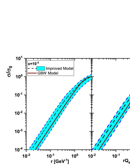
Figure 6: The ratio of the dipole cross sections in the improved saturation model (dashed lines) as a function of $r$ (left plot) and $rQ_{s}$ (right plot) for $x=10^{-3}$ at the NLO approximation. The solid lines are due to the GBW model [10]. The error bands are due to the statistical uncertainties from the coefficients of the parameterization of $F_{2}$ in [30].

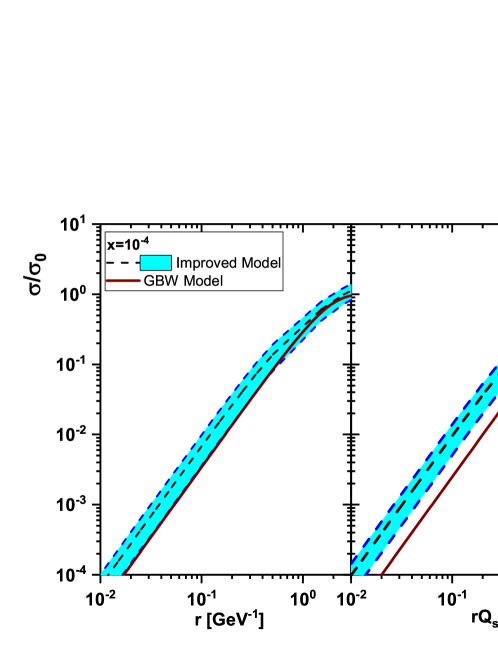
Figure 7: The same as Fig.6 for $x=10^{-4}$.

In summary, we study the unintegrated gluon distribution from a parameterization of the proton structure function. In this analysis we present the $k_{t}^{2}$-dependence of the improved UGD model at the NLO approximation and compare with four models for $f(x,k_{t}^{2})$, which exhibit rather different shape of $k_{t}$-dependence in the region, $10^{-1}{\leq}k_{t}^{2}{\leq}10^{2}~{}\mathrm{GeV}^{2}$, for a value of the longitudinal momentum fraction, $x=10^{-3}$. We show the behaviour of our predictions for the UGD are comparable with HSS and IN models in a wide range of $k_{t}^{2}$. These results are comparable with the WMR and GBW models at moderate values of $k_{t}^{2}$. It was shown that the improved UGD is different from the GBW UGD at low $k_{t}$ and it coincides with the GBW UGD at large $k_{t}$.
Then we have presented the improved dipole cross section when the unintegrated gluon distribution is derived from the parametrization of the proton structure function as a function of $r$ and $rQ_{s}$, respectively. The results according to the UGD are consistent with the GBW saturation model at the NLO approximation. The error bars are due to the statistical uncertainties of the effective parameters and preserved that the NLO results give a reasonable data description in comparison with the GBW model. In this method, the large dipole size part of the dipole cross section retains the features of the GBW model with the saturation scale. The dipole cross section at the small dipole size by the presence of the uninetrgated gluon distribution is modified in comparison with the saturation scale of the GBW saturation model.

.4 ACKNOWLEDGMENTS

The author is grateful to Razi University for the financial support of this project. I am also very grateful to the respectable reviewer of the $Eur.Phys.J.C{\bf 82},740(2022)$ article for suggesting this topic. Thanks also go to Z.Asadi for help with preparation of the UGD model.

I References

1. V.S.Fadin, E.A.Kuraev and L.N.Lipatov, Phys.Lett.B 60, 50(1975); L.N.Lipatov, Sov.J.Nucl.Phys. 23, 338(1976); I.I.Balitsky and L.N.Lipatov, Sov.J.Nucl.Phys. 28, 822(1978).
2. G.Dissertori, I.G.Knowles and M.Schmelling, Quantum Chromodynamics High Energy Experiments and Theory, Oxford University Press, 2009; R.K.Ellis, W.J.Stirling and B.R.Webber, QCD and Collider Physics, Cambridge University Press, 1996.
3. A.M.Cooper-Sarkar, R.C.E.Devenish and A. De Roeck, Int.J.Mod.Phys.A13, 3385 (1998).
4. K.Kutak and A.M.Stasto, Eur.Phys.J.C 41, 343 (2005).
5. G.I.Lykasov, A.A.Grinyuk and V.A.Bednyakov, arXiv [hep-ph]:1301.5156.
6. A.D.Bolognino, F.G.Celiberto, M.Fucilla, Dmitry Yu. Ivanov, A.Papa, W.Schafer and A.Szczurek, arXiv[hep-ph]:2202.02513.
7. I.P.Ivanov and N.N.Nikolaev, Phys.Rev.D 65, 054004 (2002).
8. J.Kwiecinski, A.D.Martin and P.J.Sutton, Z.Phys.C 71, 585 (1996); Jeffrey R.Forshaw, P.N.Harriman and P.J.Sutton, J.Phys.G 19, 1616 (1993).
9. A.J.Askew, J.Kwiecinski, A.D.Martin and P.J.Sutton, Phys.Rev. D49, 4402 (1994); E.Elias, K.Golec-Biernat and Anna M.Stasto, JHEP 01, 141 (2018).
10. K.Golec-Biernat and M.W$\ddot{\mathrm{u}}$sthoff, Phys. Rev. D 59, 014017 (1998); K. Golec-Biernat and S.Sapeta, JHEP 03, 102 (2018).
11. J.Bartels, K.Golec-Biernat and H.Kowalski, Phys. Rev. D66, 014001 (2002).
12. B.Sambasivam, T.Toll and T.Ullrich, Phys.Lett.B 803, 135277 (2020).
13. J.R.Forshaw and G.Shaw, JHEP 12, 052 (2004).
14. E.Iancu, A.Leonidov and L.McLerran, Nucl.Phys.A 692, 583 (2001); Phys.Lett.B 510, 133 (2001); E.Iancu,K.Itakura and S.Munier, Phys.Lett.B 590, 199 (2004).
15. Yu.L.Dokshitzer, Sov.Phys.JETP46, 641 (1977); G.Altarelli and G.Parisi, Nucl.Phys.B 126, 298 (1977); V.N.Gribov and L.N.Lipatov, Sov.J.Nucl.Phys. 15, 438 (1972).
16. M.A.Kimber, J.Kwiecinski, A.D.Martin and A.M.Stasto, Phys.Rev.D 62, 094006 (2000).
17. N.N.Nikolaev and B.G.Zakharov, Phys.Lett.B 332, 184 (1994); N. N. Nikolaev and W. Sch$\ddot{a}$fer, Phys. Rev. D 74, 014023 (2006).
18. R.Boussarie and Y.Mehtar-Tani, Phys.Lett.B 831, 137125 (2022).
19. I.V. Anikin, A. Besse, D.Yu. Ivanov, B. Pire, L. Szymanowski and S. Wallon, Phys. Rev. D 84, 054004 (2011).
20. M. Hentschinski, A. Sabio Vera and C. Salas, Phys. Rev. Lett. 110, 041601 (2013).
21. G. Watt, A.D. Martin and M.G. Ryskin, Eur. Phys. J. C 31, 73 (2003).
22. A.D.Bolognino, F.G.Celiberto, Dmitry Yu. Ivanov and A.Papa, arXiv [hep-ph]:1808.02958; arXiv [hep-ph]:1902.04520; arXiv [hep-ph]:1808.02395.
23. F.G.Celiberto, Nuovo Cim. C 42, 220 (2019).
24. F.G.Celiberto, D. Gordo Gomez and A.Sabio Vera, Phys.Lett.B 786, 201 (2018).
25. L.P.Kaptari, A.V.Kotikov, N.Yu.Chernikova, and P.Zhang, Phys.Rev.D 99, 096019 (2019).
26. J. Blumlein, V. Ravindran and W. van Neerven, Nucl. Phys. B 586, 349(2000); S.Catani and F.Hautmann, Nucl.Phys.B427, 475(1994).
27. D.I.Kazakov and A.V.Kotikov, Phys.Lett.B291, 171(1992); E.B.Zijlstra and W.L.van Neerven, Nucl.Phys.B383, 525(1992).
28. M.M. Block, L.Durand, P.Ha, D.W.McKay, Eur.Phys.J.C 69, 425 (2010).
29. G.R.Boroun, Eur.Phys.J.C 82, 740 (2022); G.R.Boroun, Eur.Phys.J.C 83, 42 (2023).
30. M. M. Block, L. Durand and P. Ha, Phys. Rev.D89, no. 9, 094027 (2014).