On the Numerical Integration of Singular Initial and Boundary Value Problems for Generalised Lane–Emden and Thomas–Fermi Equations

Abstract

We propose a geometric approach for the numerical integration of singular initial and boundary value problems for (systems of) quasi-linear differential equations. It transforms the original problem into the problem of computing the unstable manifold at a stationary point of an associated vector field and thus into one which can be solved in an efficient and robust manner. Using the shooting method, our approach also works well for boundary value problems. As examples, we treat some (generalised) Lane–Emden equations and the Thomas–Fermi equation.

url]http://www.mathematik.uni-kassel.de/ seiler

1 Introduction

The Lane–Emden equation was originally derived in astrophysics [1, p. 40] and represents a dimensionless form of Poisson’s equation for the gravitational potential of a Newtonian self-gravitating, spherically symmetric, polytropic fluid (see [2, 3, 4] and references therein for a more detailed discussion):

$$u^{\prime\prime}+\frac{2}{x}u^{\prime}=-u^{n}$$ (1)

with $n$ the polytropic index. Astrophysicists need the solution of the initial value problem $u(0)=1$ and $u^{\prime}(0)=0$. Eq. (1) is prototypical for ordinary differential equations arising in the construction of radially symmetric steady state solutions of reaction-diffusion equations, as the left hand side of (1) represents the Laplace operator in spherical coordinates. In an $N$-dimensional space, the numerator $2$ has to be replaced by $N-1$. This leads to generalised Lane–Emden equations of the form

$$u^{\prime\prime}+\frac{N-1}{x}u^{\prime}=h(x,u)\;,$$ (2)

where the function $h$ represents the reaction term. Besides the classical form from astrophysics, we will later consider examples arising in chemical engineering (biocatalysts) and in physiology (oxygen uptake of cells). There, one needs the solution of boundary value problems with $u^{\prime}(0)=0$ and $\alpha u(1)+\beta u^{\prime}(1)=\gamma$.

Thomas [5] and Fermi [6] derived independently of each other in a statistical model of atoms treating electrons as a gas of particles a Lane–Emden equation (1) with polytropic index $n=3/2$ for the electrostatic potential $V(x)$, however with the “initial condition” that $V(x)$ behaves like $1/x$ for $x\to 0$. Writing $V(x)=u(x)/x$, one obtains the Thomas–Fermi equation

$$u^{\prime\prime}=\sqrt{u^{3}/x}$$ (3)

together with the initial condition $u(0)=1$ (see [7, 8, 9] for more physical and historical details and [10, 11] for a mathematical analysis). In addition, one imposes one of the following three types of boundary conditions:

$$bu^{\prime}(b)-u(b)=0\;,$$ (4a)

$$\!\!\lim_{x\to\infty}u(x)=0\;,$$ (4b)

$$u(a)=0$$ (4c)

with $0<a,b<\infty$ given positions. The infinite case (4b) occurs only for a critical value $\omega\approx-1.588\dots$ of the initial slope $u^{\prime}(0)$ and represents physically an isolated neutral atom. For larger initial slopes, one can prescribe the boundary condition (4a) and obtains solutions going through a minimum and then growing rapidly. Physically, such solutions are relevant for certain crystals. The boundary condition (4c) leads to solutions with a smaller initial slope and represent physically ions with radius $a$.

Numerical methods from textbooks cannot be directly applied here, as all considered equations are singular at $x=0$ and at least one initial/boundary condition is imposed there. In the vast literature on the numerical integration of Lane–Emden and Thomas–Fermi equations, three different types of approaches prevail. For initial value problems, astrophysicists apply a very simple approach based on a series expansion of the solution to get away from the singularity and then some standard integrator [3, Sect. 7.7.2] (see also [12]). For boundary value problems, collocation methods are popular, as they are easily adapted to the singularity [13]. Finally, various kinds of semi-analytic expansions like Adomian decomposition have been adapted to the singularity (see the references given below and references therein).

We propose here a new and rather different alternative. In the geometric theory of differential equations [14, 15], one associates with any implicit ordinary differential equation a vector field on a higher-dimensional space such that the graphs of prolonged solutions of the implicit equation are integral curves of this vector field. Most of the literature on singularity theory is concerned with fully implicit equations. However, in real life applications quasi-linear equations like the Lane–Emden equations prevail. In [16, 17], the authors showed that such equations possess a special geometry allowing us to work in a lower order. Singularities, now called impasse points, are typically stationary points of the associated vector field. If there is a unique solution, its prolonged solution graph is the one-dimensional unstable manifold of this stationary point. Such an unstable manifold can numerically be computed very robustly. In [18], we already sketched this possibility to exploit ideas from singularity theory for numerical analysis. Here, we want to demonstrate for concrete problems of practical relevance that it is easy to apply and efficiently provides accurate results.

The paper is structured as follows. In the next section, we recall the necessary elements of the geometric theory of differential equations and how one can translate an implicit problem into an explicit one. Section 3 is then devoted to the application of these ideas to (generalised) Lane–Emden equations and to the numerical solution of some concrete problems from the literature. In Section 4 we discuss the Thomas–Fermi equation by first reducing it via a transformation introduced by Majorana and then applying the geometric theory. We compare the obtained numerical results with some high precision calculations from the literature. Finally, some conclusions are given.

2 Geometric Theory of Ordinary Differential Equations

We use a differential geometric approach to differential equations. It is beyond the scope of this article to provide deeper explanations of it; for this we refer to [19] and references therein. For notational simplicity, we concentrate on the scalar case; the extension to systems will be briefly discussed at the end. Similarly, we restrict here to second-order equations, but equations of arbitrary order can be treated in an analogous manner.

We consider a fully implicit differential equation of the form

$$F(x,u,u^{\prime},u^{\prime\prime})=0\;.$$ (5)

In the second-order jet bundle $\mathcal{J}_{2}$ (intuitively expressed, this is simply a four-dimensional affine space with coordinates called $x,u,u^{\prime},u^{\prime\prime}$), this equation defines a hypersurface $\mathcal{R}_{2}\subset\mathcal{J}_{2}$ which represents our geometric model of the differential equation. We will assume throughout that $\mathcal{R}_{2}$ is actually a submanifold.

Given a function $\psi(x)$, we may consider its graph as a curve in the jet bundle $\mathcal{J}_{0}$ of order zero, i. e. the $x$-$u$ space, given by the map $x\mapsto\bigl{(}x,\psi(x))$. Assuming that $\psi$ is at least twice differentiable, we can prolong this curve to a curve in $\mathcal{J}_{2}$ defined by the map $x\mapsto\bigl{(}x,\psi(x),\psi^{\prime}(x),\psi^{\prime\prime}(x)\bigr{)}$. The function $\psi$ is a solution of (5), if and only if this curve lies completely in the hypersurface $\mathcal{R}_{2}$.

In an initial value problem for the implicit equation (5), one prescribes a point $\rho=(y,u_{0},u_{1},u_{2})\in\mathcal{R}_{2}$ and asks for solutions such that $\rho$ lies on their prolonged graphs. Note that opposed to explicit problems, we must also specify the value $u_{2}$, as the algebraic equation $F(y,u_{0},u_{1},u^{\prime\prime})=0$ may have several (possibly infinitely many) solutions and thus may not uniquely determine $u_{2}$.

A key ingredient of the geometry of jet bundles is the contact structure. In the case of $\mathcal{J}_{2}$, the contact distribution $\mathcal{C}^{(2)}$ is spanned by the two vector fields

$$C_{\mathrm{trans}}=\partial_{x}+u^{\prime}\partial_{u}+u^{\prime\prime}\partial_{u^{\prime}}\;,\quad C_{\mathrm{vert}}=\partial_{u^{\prime\prime}}\;.$$ (6)

A curve $x\mapsto\bigl{(}x,\psi_{0}(x),\psi_{1}(x),\psi_{2}(x)\bigr{)}$ in $\mathcal{J}_{2}$ is a prolonged graph (i. e. $\psi_{1}=\psi_{0}^{\prime}$ and $\psi_{2}=\psi_{0}^{\prime\prime}$), if and only if all its tangent vectors lie in the contact distribution.

The Vessiot distribution $\mathcal{V}[\mathcal{R}_{2}]$ of (5) is that part of the tangent space of $\mathcal{R}_{2}$ which also lies in the contact distribution $\mathcal{C}^{(2)}$. Writing $X=aC_{\mathrm{trans}}+bC_{\mathrm{vert}}$ for a general vector in the contact distribution, $X$ lies in the Vessiot distribution, if and only if its coefficients $a,b$ satisfy the linear equation

$$\bigl{(}F_{x}+u^{\prime}F_{u}+u^{\prime\prime}F_{u^{\prime}}\bigr{)}a+F_{u^{\prime\prime}}b=0\;.$$ (7)

A singularity is a point $\rho=(y,u_{0},u_{1},u_{2})\in\mathcal{R}_{2}$ such that $F_{u^{\prime\prime}}(\rho)=0$. One speaks of a regular singularity, if the coefficient of $a$ in (7) does not vanish at $\rho$, and of an irregular singularity, if it does. Outside of irregular singularities, the Vessiot distribution is one-dimensional and locally spanned by the vector field

$$X=F_{u^{\prime\prime}}C_{\mathrm{trans}}-\bigl{(}F_{x}+u^{\prime}F_{u}+u^{\prime\prime}F_{u^{\prime}}\bigr{)}C_{\mathrm{vert}}$$ (8)

(note that $X$ is defined only on the submanifold $\mathcal{R}_{2}\subset\mathcal{J}_{2}$). The prolonged graph of any solution of (5) must be integral curves of this vector field. The converse is not necessarily true in the presence of singularities.

At regular singularities, the vector field $X$ becomes vertical. Generically, only one-sided solutions exist at such points and if two-sided solutions exist, then their third derivative will blow up [20, Thm. 4.1]. At irregular singularities, typically several (possibly infinitely many) solutions exist. In [21] it is shown how for arbitrary systems of ordinary or partial differential equations with polynomial nonlinearities all singularities can be automatically detected.

Irregular singularities are stationary points of $X$. Prolonged solution graphs through them are one-dimensional invariant manifolds. Any one-dimensional (un)stable or centre manifold (with transversal tangent vectors) at such a stationary point defines a solution. For higher-dimensional invariant manifolds, one must study the induced dynamics on them to identify solutions. In any case, we note that the numerical determination of invariant manifolds at stationary points is a well-studied topic – see e. g. [22, 23].

In general, the direct numerical integration of (5) faces some problems, if it is not possible to solve (uniquely) for $u^{\prime\prime}$, and typically breaks down, if one gets too close to a singularity. The geometric theory offers here as alternative the numerical integration of the dynamical system defined by the vector field $X$. Thus an implicit problem is transformed into an explicit one! The price one has to pay is an increase of the dimension: while (5) is a scalar equation (but second-order), the vector field $X$ lives on the three-dimensional manifold $\mathcal{R}_{2}$ in the four-dimensional jet bundle $\mathcal{J}_{2}$ (more generally, a scalar equation of order $q$ leads to a vector field on a $(q-1)$-dimensional manifold).

The key difference is, however, that we obtain a parametric solution representation. We work now with the explicit autonomous system

$$\frac{dx}{ds} =F_{u^{\prime\prime}}\;, \frac{du}{ds} =u^{\prime}F_{u^{\prime\prime}}\;,$$ (9)

$$\frac{du^{\prime}}{ds} =u^{\prime\prime}F_{u^{\prime\prime}}\;,\qquad \frac{du^{\prime\prime}}{ds} =-F_{x}-u^{\prime}F_{u}-u^{\prime\prime}F_{u^{\prime}}\;,$$

where $s$ is some auxiliary variable used to parametrise the integral curves of $X$. A solution of it will thus be a curve $s\mapsto\bigl{(}x(s),u(s),u^{\prime}(s),u^{\prime\prime}(s)\bigr{)}$ on $\mathcal{R}_{2}\subset\mathcal{J}_{2}$. A numerical integration will provide a discrete approximation of this curve.

In applications, quasi-linear equations prevail. We restrict here even to semi-linear differential equations of the form

$$F(x,u,u^{\prime},u^{\prime\prime})=g(x)u^{\prime\prime}-f(x,u,u^{\prime})=0\;,$$ (10)

with smooth functions $f$, $g$, as both the Lane–Emden and the Thomas–Fermi equation can be brought into this form. A point $(y,u_{0},u_{1},u_{2})\in\mathcal{R}_{2}$ is then a singularity, if and only if $g(y)=0$.

As first shown in [16] and later discussed in more details in [17], quasi-linear equations possess their own special geometry, as it is possible to project the Vessiot distribution to the jet bundle of one order less, i. e. in our case to the first-order jet bundle $\mathcal{J}_{1}$ with coordinates $(x,u,u^{\prime})$. Projecting the vector field $X$ defined by (8) with $F$ as in (10) to $\mathcal{J}_{1}$ yields the vector field

$$Y=g(x)\partial_{x}+g(x)u^{\prime}\partial_{u}+f(x,u,u^{\prime})\partial_{u^{\prime}}\;.$$ (11)

It is only defined on the canonical projection of $\mathcal{R}_{2}$ to $\mathcal{J}_{1}$ which may be a proper subset. Assuming that $f$, $g$ are defined everywhere on $\mathcal{J}_{1}$, we analytically extend $Y$ to all of $\mathcal{J}_{1}$ and replace (9) by the three-dimensional system

$$\frac{dx}{ds}=g(x)\;,\quad\frac{du}{ds}=g(x)u^{\prime}\;,\quad\frac{du^{\prime}}{ds}=f(x,u,u^{\prime})\;.$$ (12)

The first equation is decoupled and can be interpreted as describing a change of the independent variable, but we will not pursue this point of view.

A point $\rho=(y,u_{0},u_{1})\in\mathcal{J}_{1}$ is an impasse point for (10), if the vector field $Y$ is not transversal at $\rho$, i. e. if its $x$-component vanishes. Here, this is equivalent to $g(y)=0$. We call $\rho$ a proper impasse point, if $\mathcal{R}_{2}$ contains points which project on $\rho$; otherwise, $\rho$ is improper. Here, proper impasse points are obviously stationary points of $Y$ or (12), respectively. Prolonged graphs of solutions of (10) are one-dimensional invariant manifolds of $Y$ (or (12), resp.) and again the converse is not necessarily true. In [17], we proved geometrically the following result (a classical analytic proof for the special case $g(x)=x$ can be found in [24]).

Theorem 1.

Consider (10) for $f,g$ smooth together with the initial conditions $u(y)=u_{0}$ and $u^{\prime}(y)=u_{1}$ where $g(y)=0$ and $f(y,u_{0},u_{1})=0$. If $\delta=g^{\prime}(y)$ and $\gamma=f_{u^{\prime}}(y,u_{0},u_{1})$ are both non zero and of opposite sign, then the initial value problem possesses a unique smooth solution.

Under the made assumptions, the initial point $\rho=(y,u_{0},u_{1})$ is a proper impasse point of (10). One readily verifies that the Jacobian $J$ of $Y$ at $\rho$ has the eigenvalues $\delta$, $0$ and $\gamma$ and thus we find three one-dimensional invariant manifolds at $\rho$: the stable, the unstable and the centre manifold. Without loss of generality, we assume that $\delta>0$ (otherwise we multiply (10) by $-1$). It is then shown in [17] that the prolonged graph of the unique solution is the unstable manifold and thus at $\rho$ it is tangent to the eigenvector of $J$ for $\delta$.

Remark 2.

The extension to implicit systems $\mathbf{F}(x,\mathbf{u},\mathbf{u}^{\prime},\mathbf{u}^{\prime\prime})=0$ is straightforward. Assuming that the unknown function $\mathbf{u}$ is vector valued, $\mathbf{u}\colon\mathcal{I}\subseteq\mathbbm{R}\to\mathbbm{R}^{n}$, the jet bundle $\mathcal{J}_{2}$ is $(3n+1)$-dimensional and the contact distribution $\mathcal{C}^{(2)}$ is generated by the $n+1$ vector fields $C_{\mathrm{trans}}=\partial_{x}+\mathbf{u}^{\prime}\cdot\partial_{\mathbf{u}}+\mathbf{u}^{\prime\prime}\cdot\partial_{\mathbf{u}^{\prime}}$ and $\mathbf{C}_{\mathrm{vert}}=\partial_{\mathbf{u}^{\prime\prime}}$, where the dot denotes the standard scalar product. Again the Vessiot distribution is generically one-dimensional and the coefficients of a vector field $X$ spanning it are readily determined by solving a linear system of equations. Numerical integration of $X$ allows us to approximate solutions of the given system.

We restrict to semi-linear first-order systems of the form $g(x)\mathbf{u}^{\prime}=\mathbf{f}(x,\mathbf{u})$ with $g$ still a scalar function. For initial conditions $\mathbf{u}(y)=\mathbf{u}_{0}$ with $g(y)=0$ and $\mathbf{f}(y,\mathbf{u}_{0})=0$, we introduce $\delta=g^{\prime}(y)$ (assuming $\delta>0$) and the Jacobian $\Gamma=\mathbf{f}_{\mathbf{u}}(y,\mathbf{u}_{0})$. In [26], it is shown that if all eigenvalues of $\Gamma$ have a negative real part, then the initial value problem has a unique smooth solution. A classical analytical proof was given by Vainikko by first studying extensively the linear case [27] and then extending to the nonlinear one [28]. In the geometric approach, one sees again that the graph of the solution is a one-dimensional unstable manifold of the vector field $Y$ spanning the projected Vessiot distribution.

3 (Generalised) Lane–Emden Equations

3.1 Geometric Treatment

If we consider the generalised Lane–Emden equation (2), then one obtains after multiplication by $x$ the special case of (10) given by

$$g(x)=x\;,\qquad f(x,u,u^{\prime})=xh(x,u)-(N-1)u^{\prime}\;,$$ (13)

where we always assume $N>1$. For arbitrary initial conditions $u(0)=u_{0}$ and $u^{\prime}(0)=u_{1}$, we find that $\delta=1$ and $\gamma=-(N-1)$ are nonzero and of opposite sign. The initial point $\rho=(0,u_{0},u_{1})$ is a proper impasse point, if and only if $u_{1}=0$. In this case, Theorem 1 asserts the existence of a unique smooth solution.

The projected Vessiot distribution is spanned by the vector field

$$Y=x\partial_{x}+xu^{\prime}\partial_{u}+\bigl{[}xh(x,u)-(N-1)u^{\prime}\bigr{]}\partial_{u^{\prime}}\;.$$ (14)

For $u_{1}\neq 0$, no solution can exist. Indeed, the vector field $Y$ has then no stationary point and the unique trajectory through the initial point $\rho=(0,u_{0},u_{1})$ is the vertical line $s\mapsto(0,u_{0},u_{1}+s)$ which does not define a prolonged graph.

We thus assume $u_{1}=0$, which unsurprisingly is the case in all applications of (2) in the literature. Independent of the value of $u_{0}$, the initial point $\rho=(0,u_{0},0)$ is a stationary point of the vector field $Y$. The Jacobian of $Y$ at $\rho$ is

$$J=\begin{pmatrix}1&0&0\\ 0&0&0\\ h(0,u_{0})&0&-(N-1)\end{pmatrix}\;.$$ (15)

Its eigenvalues are $1$, $0$ and $-(N-1)$. Relevant for us is only the eigenvector to the eigenvalue $1$, as it is tangential to the unstable manifold. It is given by $\mathbf{v}=\bigl{(}N,0,h(0,u_{0})\bigr{)}^{T}$.

For the numerical solution of our given initial value problem, we integrate the vector field $Y$ for the initial data $\bigl{(}x(0),u(0),u^{\prime}(0)\bigr{)}^{T}=\bigl{(}0,u_{0},0\bigr{)}^{T}+\epsilon\mathbf{v}$ with some small $\epsilon>0$. The concrete value of $\epsilon$ is not very relevant. As the exact solution corresponds to the unstable manifold, any error is automatically damped by the dynamics of $Y$. In our experiments, we typically used $\epsilon=10^{-3}$ or $\epsilon=10^{-4}$.

We can easily extend this approach to coupled systems of the form

$$\mathbf{u}^{\prime\prime}+\frac{N-1}{x}\mathbf{u}^{\prime}=\mathbf{h}(x,\mathbf{u})\;,$$ (16)

where $\mathbf{u}$ is a vector valued function and the coupling occurs solely through the reaction terms. If $\mathbf{u}$ is a $d$-dimensional vector, then the dimension of the first-order jet bundle $\mathcal{J}_{1}$ is $2d+1$. Thus (12) becomes a system of this dimension:

$$\frac{dx}{ds}=x\;,\quad\frac{d\mathbf{u}}{ds}=x\mathbf{u}^{\prime}\;,\quad\frac{d\mathbf{u}^{\prime}}{ds}=x\mathbf{h}(x,\mathbf{u})-(N-1)\mathbf{u}^{\prime}\;.$$ (17)

By the same arguments as in the scalar case, we restrict to the initial condition $\mathbf{u}^{\prime}(0)=\mathbf{0}$ so that the initial point $\rho=(0,\mathbf{u}_{0},\mathbf{0})$ is again a proper impasse point. The Jacobian at $\rho$ is a block form of (15):

$$J=\begin{pmatrix}1&\mathbf{0}^{T}&\mathbf{0}^{T}\\ \mathbf{0}&0_{d}&0_{d}\\ \mathbf{h}(0,\mathbf{u}_{0})&0_{d}&-(N-1)E_{d}\end{pmatrix}\;,$$ (18)

where $0_{d}$ and $E_{d}$ denote the $d\times d$ zero and unit matrix, resp. We still have $1$ as a simple eigenvalue, whereas the eigenvalues $0$ and $-(N-1)$ have both the algebraic multiplicity $d$. The $d$-dimensional stable and centre manifolds are again vertical and irrelevant for a solution theory. But we still find a one-dimensional unstable manifold corresponding to the prolonged graph of the unique solution. It is tangential to the vector $\mathbf{v}=\bigl{(}N,\mathbf{0}^{T},\mathbf{h}(0,\mathbf{u}_{0})^{T}\bigr{)}^{T}$ and as in the scalar case we use as initial data for its determination the point $\bigl{(}0,\mathbf{u}_{0}^{T},\mathbf{0}^{T}\bigr{)}^{T}+\epsilon\mathbf{v}$.

3.2 Numerical Results

As our main goal consists of showing how easy the numerical integration of singular problems becomes with our geometric approach, we did not develop any sophisticated production code. We performed all our computations with the built-in numerical capabilities of Maple. We used most of the time the dsolve/numeric command with its standard settings, i. e. a Runge–Kutta–Fehlberg pair of order 4/5 is applied with a tolerance of $10^{-6}$ for the relative error and $10^{-7}$ for the absolute error.

Our geometric ansatz does not determine approximations $u_{n}\approx u(x_{n})$ of the solution $u(x)$ on a discrete mesh $(x_{n})$, but approximations $x_{n}=x(s_{n})$ and $u_{n}=u(s_{n})$ for a parametric representation $\bigl{(}x(s),u(s)\bigr{)}$ of the graph of the solution. Hence, for computing an approximated solution value $u(\bar{x})$, one must first determine a parameter value $\bar{s}$ such that $x(\bar{s})\approx\bar{x}$. This can easily be accomplished either with a nonlinear solver or with a numerical integrator with event handling. We used the latter option in most of our experiments.

For boundary value problems, we applied the shooting method which worked very well. Since Maple provides no built-in command for it, we wrote our own simple version. In scalar problems, we solved the arising nonlinear equation most of the time with the Steffensen method (with Aitken $\Delta^{2}$ acceleration). As our equations are dimension-free, suitable starting values were easy to find: typically, $u(x)$ varied between $0$ and $1$ and we simply chose the midpoint $0.5$.

We encountered difficulties only in the simulation of a biocatalyst. For some parameter values, the correct initial value was very close to zero and the Steffensen iterations produced sometimes intermediate approximations which were negative and for which the numerical integration became meaningless. Here we resorted to a simple bisection method.

For Lane–Emden systems, we used the Newton method for the arising nonlinear systems. The Jacobian was determined via the variational equation of the differential system. Thus for an $n$-dimensional differential system where $k<n$ initial conditions have to be determined via shooting, we had to solve an additional $kn$-dimensional linear differential system with variable coefficients.

3.2.1 Scalar Lane–Emden Equations

We consider scalar Lane–Emden equations of the generalised form

$$u^{\prime\prime}+\frac{m}{x}u^{\prime}=f(x,u)$$ (19a)

together with either the initial conditions

$$u(0)=u_{0}\;,\quad u^{\prime}(0)=0$$ (19b)

or the boundary conditions

$$u^{\prime}(0)=0\;,\quad\alpha u(1)+\beta u^{\prime}(1)=\gamma\;.$$ (19c)

Chawla and Shivakumar [29] proved for boundary value problems with $\alpha=1$ and $\beta=0$ an existence and uniqueness theorem under the following assumption on the right hand side $f(x,u)$: the supremum $M$ of the negative partial derivative $-f_{u}(x,u)$ on $[0,1]\times\mathbbm{R}$ must be less than the first positive root $t_{1}$ of the Bessel function $J_{(m-1)/2}(\sqrt{t})$ (in the frequent case $m=2$, we thus need $M<\pi^{2}$).

The numerical integration of (19a) has been studied by many authors using many different approaches; we refer to [30] for an overview of many works before 2010. We will discuss three different situations: (i) initial value problems in astrophysics, (ii) Dirichlet boundary value problem in chemical engineering and (iii) mixed boundary value problems in physiology.

Initial Value Problems from Astrophysics

In the classical Lane–Emden equations, one has $m=N-1$ with $N$ the space dimension and $f(x,u)=-u^{n}$. The solutions for $u_{0}=1$ are known as polytropes. Physically meaningful is the range $0\leq n<5$ (with $n$ not necessarily an integer). For three polytropic indices, namely $n=0,1,5$, exact solutions are known [4, Sect. 2.3]. Of physical relevance are in particular the first zero $\xi_{1}$ of $u$ (corresponding to the scaled radius of the sphere) and the value of $u^{\prime}(\xi_{1})$ (e. g. the ratio of the central density to the mean density is given by $r=-\xi_{1}/3u^{\prime}(\xi_{1})$).

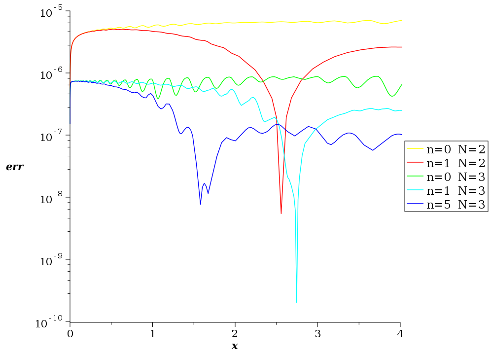
Figure 1: Logarithmic plot of absolute deviation from exact solution for some polytropes.

We numerically solved the Lane–Emden equations by integrating the dynamical system (12) with $f,g$ given by (13). As concrete test cases, we used some polytropic cylinders and spheres where the exact solutions are known. Figure 1 shows the observed errors in logarithmic scale. Obviously, the results are within the expected range for the default settings of Maple’s numerical integrator.

$N,\ n$	$\xi_{1}$	$r$
$2,\ 0$	$3.2\cdot 10^{-6}$	$4.0\cdot 10^{-7\phantom{0}}$
$2,\ 2$	$4.2\cdot 10^{-7}$	$5.7\cdot 10^{-6\phantom{0}}$
$3,\ 0$	$4.3\cdot 10^{-7}$	$2.2\cdot 10^{-10}$
$3,\ 1$	$1.5\cdot 10^{-7}$	$9.3\cdot 10^{-7\phantom{0}}$

Table 1: Relative errors for first zero $\xi_{1}$ and density ratio $r$ for the cases with $\xi_{1}<\infty$.

Our approach also determines approximations $u_{n}^{\prime}=u^{\prime}(s_{n})$ for the first derivatives of the solution, as the integral curves of the vector field $Y$ define a parametrisation $\bigl{(}x(s),u(s),u^{\prime}(s)\bigr{)}$ of the solution and its first derivative. We use this to approximate also the quantities $\xi_{1}$ and $r$. Table 1 exhibits their relative errors compared with the exact solution for those cases where $\xi_{1}$ is finite. Again, the observed accuracy corresponds well to the settings of the numerical integrator.

Boundary Value Problems for Biocatalysts

In chemical engineering, the Lane–Emden equation arises in the analysis of diffusive transport and chemical reactions of species inside a porous catalyst pellet [31, §6.4] with boundary conditions of the form (19c) with $\alpha=\gamma=1$ and $\beta=0$. Flockerzi and Sundmacher [32] considered the case $m=2$ and $f(x,u)=\phi^{2}u^{n}$ for a single species obeying Fick’s law with constant diffusivity and power-law kinetics (the constant $\phi^{2}$ is the Thiele modulus describing the ratio of surface reaction rate to diffusion rate). As this corresponds up to a sign exactly to the above considered polytropes, we omit concrete calculations and only note that [32] also provides a nice geometric proof of the existence of a unique solution of this particular boundary value problem which, unfortunately, seems not be extendable to other functions $f$.

Using a Michaelis–Menten kinetics for a biocatalyst, one obtains right hand sides like $f(x,u)=9\phi^{2}\tfrac{u}{1+Ku}$, where $\phi$ is again the Thiele modulus and $K$ the dimensionless Michaelis–Menten constant (see [33] for some further variants). This model was analysed by a homotopy perturbation method in [34]. A quantity relevant for engineers is the effectiveness factor which is here given by $\eta=\tfrac{K+1}{3\phi^{2}}u^{\prime}(1)$. A numerical study of the dependency of $\eta$ on $\phi^{2}$ and $K$ leads to the surface shown in Fig. 2 based on a $17\times 17$ grid, i. e. on the numerical solution of 289 boundary value problems with different combinations of parameter values. As indicated above, we had to use here a bisection method for locating the right initial value. Bisecting until an interval length of $10^{-5}$ was reached, the whole computation required only 2–3sec on a laptop (equipped with eight Intel Core i7-11370H (11th generation) working with 3.3GHz and 16GB of RAM running Maple 2022 under Windows 11).

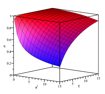
Figure 2: Dependency of the effectiveness factor $\eta$ on Thiele modulus $\phi^{2}$ and dimensionless Michaelis–Menten constant $K$.

Matlab’s solvers bvp4c and bvp5c are finite difference methods based on a three- and four-stage, resp., Lobatto IIIa collocation formulae and provide a special option for the type of singularity appearing in Lane–Emden equations [35, 36]. However, it turned out to be nontrivial to determine a plot like Fig. 2 with them, as for some parameter values they react rather sensitive to the required initial guess. Using a simple constant function lead sometimes either to completely wrong solutions or the collocation equations could not be solved. We then computed one solution with “harmless” parameter values and used it as initial guess for all other parameter values. But the computations required with 5–6sec about twice as much time as our approach.

An alternative approach consists in transforming the problem into a reaction-diffusion equation by adding a time derivative. The desired solution of our boundary value problem arises then as asymptotic for long times. Matlab provides here with pdepe a specialised solver admitting again our type of singularity. It employs a method for parabolic partial differential equations proposed by Skeel and Brezins [37] using a spatial discretisation derived with a Galerkin approach. Here, one does not need an initial guess and it turns out that a steady state is reached very rapidly (already $t=1$ is sufficient). But one needs an additional interpolation with pdeval to determine derivative values. Furthermore, the computation time for a plot like Fig. 2 increases significantly to about 17sec.

Mixed Boundary Conditions for a Physiological Model

The same differential equation is used to model the steady state oxygen diffusion in a spherical cell with Michaelis-Menten uptake kinetics [38, 39], $m=2$ and $f(x,u)=\tfrac{au}{u+K}$, but with mixed boundary conditions (19c) where $\alpha=\gamma$, $\beta=1$. Hiltmann and Lory [40] proved explicitly the existence and uniqueness of a solution of this problem. In the first two references above, concrete, physiologically meaningful values for the parameters are determined and numerical results are presented which are, however, contradictory. We used for our experiments four different parameter sets proposed by McElwain [39] and which can be found in Table 2.

	$a$	$K$	$\alpha$
1	$0.38065$	$0.03119$	$5$
2	$0.38065$	$0.03119$	$0.5$
3	$0.76129$	$0.03119$	$5$
4	$0.38065$	$0.31187$	$5$

Table 2: Parameter values for the oxygen uptake model following McElwain [40].

In particular for the third parameter set, several authors performed similar computations starting with Hiltmann und Lory [40]. Khuri and Sayfy [41, Ex. 3] combined a decomposition method in the vicinity of the singularity with a collocation method in the rest of the integration interval. They provided – like Hiltmann and Lory – approximations of $u(x_{i})$ for $x_{i}=i/10$ with $i=0,\dots,10$ [41, Tbl. 5] and compared with results of Çağlar et al. [42]. It turned out that for the first six digits all three approaches and our method yield exactly the same result – a quite remarkable agreement. Fig. 3 provides plots of the oxygen concentration $u(x)$ and of its rate of change $v(x)=u^{\prime}(x)$ for all four different sets of parameters as obtained by our method. The concentration plot agrees well with the one given by McElwain [39, Fig. 1] (and confirmed by Hiltmann und Lory [40]).

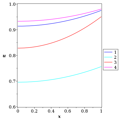
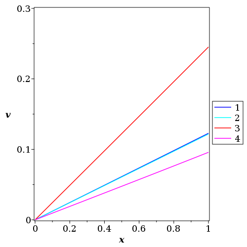
Figure 3: Numerical solutions of the boundary value problem for the oxygen uptake model for four different sets of parameters given in Table 2. Left: oxygen concentration $u(x)$. Right: rate of change of oxygen concentration $u^{\prime}(x)$.

Hiltmann and Lory [40] report that they used a sophisticated implementation of a multiple shooting procedure based on four different integrators for initial value problems together with a special treatment of the singularity using both a technique of de Hoog and Weiss [43] and a Taylor series method (no further details are given). They prescribed a tolerance of $10^{-8}$ for their Newton solver and $10^{-10}$ for the integrator. By contrast, we used a simple shooting method with the Maple built-in Runge–Kutta–Fehlberg integrator and a hand-coded Steffensen method for the nonlinear system with a tolerance of $10^{-7}$. This comparison again demonstrates how much simplicity and robustness one gains by using the associated vector field for the numerical integration in singular situations.

3.2.2 Lane–Emden Systems

Our approach works for systems in the same manner as for scalar equations, as one still finds a one-dimensional unstable manifold corresponding to prolonged graph of the solution. Thus we restrict to just one example of dimension $d=3$. We now have to integrate the system (17) of dimension $n=2d+1=7$ for the above given initial data. We used a Newton method for solving the nonlinear system arising in the shooting method. Since we had to determine $d=3$ initial conditions via shooting, we had to augment (17) by a linear matrix differential equation with variable coefficients of dimension $7\times 3$.

Campesi et al. [44] proposed a system of coupled Lane–Emden equations as model for the combustion of ethanol and ethyl acetate over an MnCu catalyst using a Langmuir–Hinshelwood–Hougen–Watson kinetics. In dimensionless form, the system is given by (see [45])

$$u^{\prime\prime}+\frac{2}{x}u^{\prime} =\frac{\mu_{u}u}{1+\lambda_{u}u+\lambda_{v}v+\lambda_{w}w}\;,$$ (20)

$$v^{\prime\prime}+\frac{2}{x}v^{\prime} =\frac{\mu_{v}v-\mu_{u}u}{1+\lambda_{u}u+\lambda_{v}v+\lambda_{w}w}\;,$$

$$w^{\prime\prime}+\frac{2}{x}w^{\prime} =\frac{\mu_{w}w}{1+\lambda_{u}u+\lambda_{v}v+\lambda_{w}w}\;,$$

where $u$, $v$, $w$ represent (dimensionless) molar concentrations of ethanol, acetaldehyde and ethyl acetate, respectively. The boundary conditions require that at $x=0$ all first derivatives vanish and that at $x=1$ all concentrations are $1$.

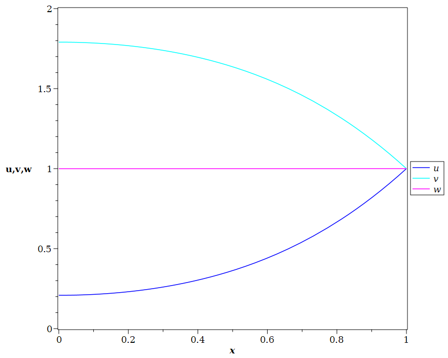
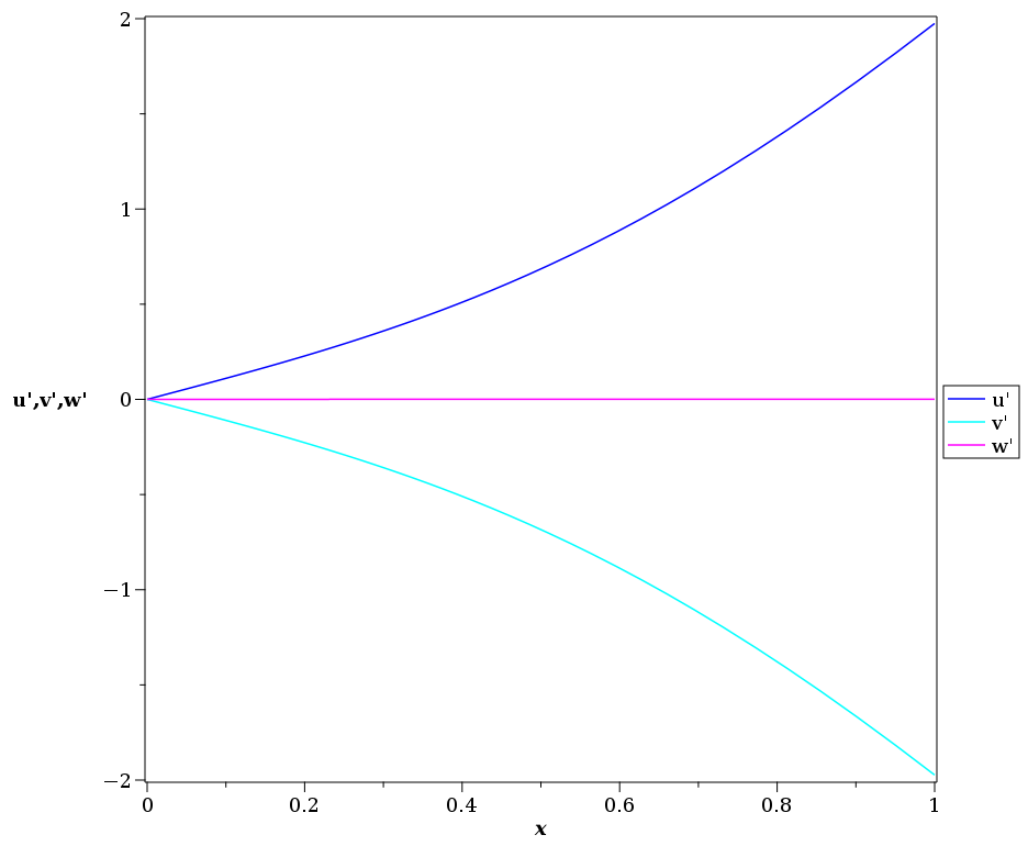
Figure 4: Numerical solutions of the boundary value problem for the dimensionless model of the MnCu catalyst. Left: concentrations of ethanol, acetaldehyde and ethyl acetate, respectively. Right: corresponding rates of change.

The authors of [44] used for numerically integrating (20) an approach developed by essentially the same group [46] based on an integral formulation and an $h$-adaptive mesh procedure. Unfortunately, [44] does not provide all the parameters used in the computations so that it is not possible to compare with their results. We used instead for our experiments data given in [45] (employing a modified Adomian decomposition method). However, the plots given there are not correct, as apparently wrong differential equations were used – at least in the Matlab code presented in the appendix. We compared with analogous Matlab computations using the right differential equations and again pdepe as a numerical solver and obtained an excellent agreement. Figure 4 presents solution curves for the values $\mu_{u}=30$, $\mu_{v/w}=0.01$, $\lambda_{u}=3$ and $\lambda_{v/w}=0.1$ used in [45].

4 Thomas–Fermi Equation

4.1 Majorana Transformation

The Thomas–Fermi equation (3) belongs also to the class (10), but with

$$g(x)=\sqrt{x}\;,\qquad f(x,u,u^{\prime})=\sqrt{u^{3}}\;.$$ (21)

The initial condition $u(0)=1$ leads to a rather different situation as for the Lane–Emden equation: the implicit form of the Thomas–Fermi equation entails that the only points on $\mathcal{R}_{2}$ which project on $x=0$ are of the form $\rho=(0,0,u_{1},u_{2})$ with arbitrary values $u_{1}$, $u_{2}$. Hence no solution satisfying the above initial condition can be twice differentiable at $x=0$. Solutions with a higher regularity exist only for the initial condition $u(0)=0$ which has no physical relevance.

Any point of the form $\rho=(0,1,u_{1})$ is an improper impasse point. The vector field $Y$ defined by (11) does not vanish at such points but takes the form $\partial_{u^{\prime}}$ and it is not Lipschitz continuous there. While Peano’s theorem still asserts the existence of solutions, we cannot apply the Picard–Lindelöf theorem to guarantee uniqueness. We could rescale $Y$ by some function like $x$ which does not change its trajectories for obtaining an everywhere differentiable vector field $\tilde{Y}=xY$. Now all points of the above form are stationary points. But the Jacobian of $\tilde{Y}$ has $0$ as a triple eigenvalue at them making it hard to analyse the local phase portrait.

We use therefore a different approach. As Esposito [47] reported only in 2002, Majorana proposed already in 1928 a differential transformation to a new independent variable $t$ and a new dependent variable $v$ of the form

$$t=144^{-1/6}x^{1/2}u^{1/6}\;,\qquad v=-(16/3)^{1/3}u^{-4/3}u^{\prime}\;.$$ (22)

This at first sight rather miraculous transformation stems from a particular kind of scaling symmetry [48]. A computation detailed in [47] shows that if it is applied to any solution of the Thomas–Fermi equation (3), then the transformed variables satisfy the reduced equation

$$(1-t^{2}v)\frac{dv}{dt}=8(tv^{2}-1)\;.$$ (23)

The boundary condition (4b), i. e. $\lim_{x\to\infty}u(x)=0$, translates into the condition $v(1)=1$. We will see below that the thus defined singular initial value problem for (23) possesses two solutions. Only one of them is also defined for $t=0$ and thus is the physically relevant one. It follows from (22) that the initial slope $u^{\prime}(0)$ for the Thomas–Fermi equation is obtained from a solution of (23) by

$$u^{\prime}(0)=-(3/16)^{1/3}v(0)\;.$$ (24)

The reduced equation (23) is quasi-linear and of first order. Opposed to the Lane–Emden equations, it is not semi-linear. Thus singular behaviour does not simply occur at specific $t$-values. Instead it appears whenever a solution graph contains a point $(t,v)$ with $t^{2}v=1$. Nevertheless, one can apply the same kind of approach. One first computes a vector field $X$ living on the hypersurface $\mathcal{R}_{1}\subset\mathcal{J}_{1}$ defined by (23) and spanning there the Vessiot distribution. Then one projects $X$ to the jet bundle $\mathcal{J}_{0}$ and obtains there the vector field

$$Y_{\mathrm{red}}=(t^{2}v-1)\partial_{t}+8(1-tv^{2})\partial_{v}\;.$$ (25)

As we are now on $\mathcal{J}_{0}$, one-dimensional invariant manifolds of $Y_{\mathrm{red}}$ which are transversal can be directly identified with the graphs of solutions of (23). Our initial point $(1,1)$ is a proper impasse point where $Y_{\mathrm{red}}$ vanishes.

Fig. 5 shows the phase portrait of the vector field $Y_{\mathrm{red}}$. It has $(1,1)$ as its only stationary point. The plot shows in blue some integral curves. Most, but not all of them can be considered as the graphs of solutions of (23). The plot also contains in red the $t$-nullcline given by $v=1/t^{2}$ – which is simultaneously the singular locus of (23) – and in green the $v$-nullcline given by $v=\pm 1/\sqrt{t}$. The integral curves that cross the $t$-nullcline show at the intersection a turning point behaviour, as the $t$-component of $Y_{\mathrm{red}}$ changes its sign there. If $(t_{i},v_{i})$ is such an intersection point, then it splits the corresponding integral curve into two solution graphs where both solutions are defined only for $t<t_{i}$, as they both loose their differentiability at $t=t_{i}$. With traditional numerical methods applied to (23), it would be difficult to determine these solutions; as integral curves of $Y_{\mathrm{red}}$ they are trivial to obtain numerically.

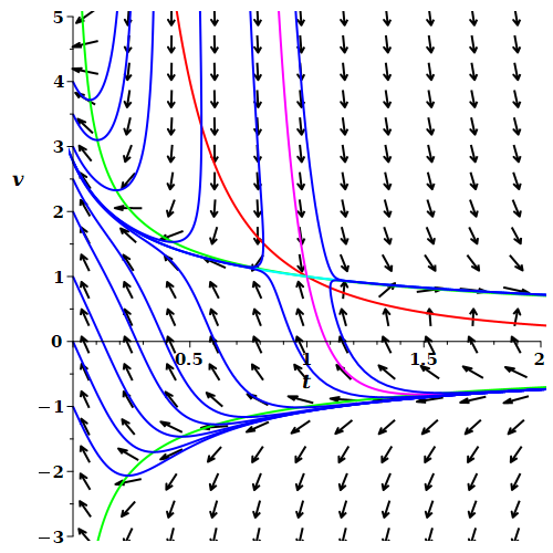
Figure 5: Phase portrait of the vector field associated to the reduced system (23). The unstable manifold is shown in cyan, the stable manifold in magenta.

The Jacobian of $Y_{\mathrm{red}}$ at the stationary point $(1,1)$ is the matrix $J=\left(\begin{smallmatrix}2&1\\ -8&-16\end{smallmatrix}\right)$ with eigenvalues $-7\pm\sqrt{73}\approx(1.544,-15.544)$. Thus we are dealing with a saddle point. The unstable and the stable manifold shown in Fig. 5 in cyan and magenta, resp., correspond to the above mentioned two solutions of the initial value problem with $v(1)=1$. There cannot exist any additional solutions, as there are no further invariant manifolds entering or leaving the saddle point. One sees that in the positive quadrant the stable manifold cannot cross the nullclines outside of the saddle point and hence can never reach the $v$-axis.

Thus we may conclude that the part of the unstable manifold between the $v$-axis and the stationary point corresponds to the unique solution $u_{\infty}$ of the boundary value problem with the condition (4b). The abscissa of the intersection of the unstable manifold with the $v$-axis determines via (24) the critical initial slope $\omega$ (see below for numerical values). The existence of such a unique solution for this specific boundary value problem was proven in 1929 by Mambriani [49] (see also the discussion in [11]).

It will turn out that the integral curves to the right of the stable manifold have no relevance for our problem. The integral curves to the left of it and above the unstable manifold correspond to solutions of the boundary value problem with the condition (4c), i. e. solutions with a zero, whereas the integral curves below the stable manifold lead to solutions for (4a). This can be deduced from their intersections with the $v$-axis and (24).

Much of the literature on numerically solving the Thomas–Fermi equation is concerned with the solution $u_{\infty}$ of (4b) defined on the semi-infinite interval $[0,\infty)$ and concentrates on the determination of the critical slope $\omega$. Most solutions reported in the literature are either shown only on rather small intervals $[0,x_{0}]$ with typically $x_{0}<10$ or clearly deteriorate for larger $x$. One reason for this effect is surely that many approaches are based on some kind of series expansion. Another, more intrinsic reason becomes apparent from the phase portrait in Figure 5. As the sought solution corresponds to a branch of the unstable manifold of the saddle point $(1,1)$, even small errors close to the saddle point (corresponding to points with large $x$ coordinates) are amplified by the dynamics and the numerical solutions tend to diverge from a finite limit.

By contrast, our approach to determine $u_{\infty}$ leads to the standard problem of determining a branch of the unstable manifold of a stationary point – a task which can be performed numerically very robustly and efficiently. As the positive eigenvalue has about the tenfold magnitude of the negative one, trajectories approach the unstable manifold very fast which ensures a high accuracy.

Following Majorana, Esposito [47] (and subsequent authors) determines a series solution of the initial value problem $v(1)=1$ for (23). In the first step, one obtains a quadratic equation with two solutions. Esposito then argues that one should take the smaller solution, as this was a perturbation calculation which is not a convincing argument. The reduced initial value problem has two solutions. As one can see in Figure 5, the second solution corresponding to the stable manifold grows very rapidly. Therefore it is not surprising that several authors suspected that the second solution of the quadratic equation leads to a divergent power series and thus could be discarded. However, a second solution to the initial value problem does exist, although it seems that it cannot be determined with a power series ansatz. But as already discussed above, $u_{\infty}$ is nevertheless unique and corresponds to the unstable manifold.

For the series solution, one expands around $t=1$ and makes the ansatz $v(t)=\sum_{i=0}^{\infty}a_{i}(1-t)^{i}$. The initial condition yields $a_{0}=1$ and for the arising quadratic equation for $a_{1}$ one chooses the root $a_{1}=9-\sqrt{73}\approx 0.456$. After lengthy computations sketched in [47], one obtains the following recursive expression for the remaining coefficients with $i>1$:

$$a_{i}=\frac{1}{2(i+8)-(i-1)a_{1}}\Biggl{[}(i+6)a_{1}a_{i-2}+\Bigl{(}(i+7)-2(i+3)a_{1}\Bigr{)}a_{i-1}+{}\\ \sum_{j=1}^{i-2}\Bigl{(}(j+1)a_{j+1}-2(j+4)a_{j}+(j+7)a_{j-1}\Bigr{)}a_{i-j}\Biggr{]}\;.$$ (26)

Setting $t=0$ yields for the critical slope the series representation

$$\omega=-\left(\frac{3}{16}\right)^{1/3}\sum_{i=0}^{\infty}a_{i}\;,$$ (27)

which can be evaluated to arbitrary precision.

To obtain whole solutions $u(x)$, one must be able to transform back from the variables $(t,v)$ to the original variables $(x,u)$. Esposito [47] exhibited a convenient method for this. We express the solution in parametric form using $t$ as parameter: $x=x(t)$ and $u=u(t)$. Then we make the ansatz

$$u(t)=\exp{\left\{\int_{0}^{t}w(\tau)d\tau\right\}}$$ (28)

with $w$ a yet to be determined function. Assuming $x(t=0)=0$, this ansatz automatically satisfies the initial condition $u(x=0)=1$. Using the transformation (22), one can show that $w(t)=\tfrac{6tv(t)}{t^{2}v(t)-1}$ and that $x(t)$ can be expressed via $w(t)$ as

$$x(t)=144^{1/3}t^{2}\exp{\left\{-\frac{1}{3}\int_{0}^{t}w(\tau)d\tau\right\}}$$ (29)

(which shows that indeed $x(0)=0$). Esposito [47] proposed to enter the above determined series solution for $v(t)$ into these formulae and to compute this way a series expansion of $u_{\infty}$. This requires essentially one quadrature.

4.2 Numerical Results

We refrain from citing the many papers written on computing $u_{\infty}$ and in particular $\omega$ and instead refer only to [50, 51] both listing a large number of approaches with references. We emphasise again that our main point is to show that the geometric theory allows us – here in combination with the Majorana transformation – to translate a singular problem into basic tasks from the theory of dynamical systems which can be easily solved by standard methods.

4.2.1 The “Critical” Solution $u_{\infty}$ and the Critical Slope $\omega$

We consider first the problem of only determining the initial slope $\omega$ belonging to the solution $u_{\infty}$ for (4b). With classical approaches, this is a non-trivial problem and in the literature one often finds values with a very low number of correct digits. Using our geometric approach, we can determine $\omega$ to (almost) any desired precision in about 10 lines of Maple code. We write the dynamical system corresponding to the vector field $Y_{\mathrm{red}}$ defined by (25) as

$$\frac{dt}{ds}=t^{2}v-1\;,\qquad\frac{dv}{ds}=8(1-tv^{2})\;,$$ (30)

i. e. we determine integral curves of $Y_{\mathrm{red}}$ in parametric form $\bigl{(}t(s),v(s)\bigr{)}$. As discussed above, the sought trajectory corresponds to the unstable manifold of the saddle point $(1,1)$. An eigenvector for the positive eigenvalue $\lambda=-7+\sqrt{73}$ is given by $\mathbf{e}=\bigl{(}1,\ -9+\sqrt{73}\bigr{)}^{T}$ and we denote by $\hat{\mathbf{e}}=(e_{1},\ e_{2})^{T}$ the corresponding normalised vector. Then we choose as initial point for a numerical integration $t(0)=1+\epsilon e_{1}$ and $v(0)=1+\epsilon e_{2}$ with $\epsilon>0$ some small number (we typically used $10^{-3}$ or $10^{-4}$, but this had no effect on the obtained slope) and integrated until $t(s)=0$ for $s=s_{0}$. Finally, we obtain $\omega$ from $v(s_{0})$ via (24).

We control the precision with an integer parameter $N$ specifying that the numerical integration of (30) should take place with an absolute and relative error of $10^{-N}$ and that for this purpose Maple should compute with $N+5$ digits. In a recent work, Fernández and Garcia [51] determined $\omega$ based on the first 5000 terms of the Majorana series (27) to a precision of several hundred digits. This is by far the best approximation available and our reference solution.

tolerance	rel. error	time
$10^{-5\phantom{0}}$	$3.2\cdot 10^{-6\phantom{0}}$	$0.6$
$10^{-10}$	$7.3\cdot 10^{-12}$	$0.6$
$10^{-15}$	$5.5\cdot 10^{-17}$	$2.7$
$10^{-20}$	$5.3\cdot 10^{-22}$	$22.7$
$10^{-25}$	$5.5\cdot 10^{-27}$	$231.5$

Table 3: Relative error and computation time in seconds for different tolerances.

Our numerical results are summarised in Table 3. Our relative error is always smaller than the prescribed tolerance. For smaller tolerances, the computational effort is rapidly increasing and on a laptop we needed for 25 digits less than 4 minutes. We made no effort to optimise the computations. For example, we are using the default integration method of Maple (a Runge–Kutta–Fehlberg method of order 4/5 with a degree four interpolant), although a higher order scheme would probably be more efficient (Maple offers such schemes – but not in combination with the automated root finding used in our code). Nevertheless, one may conclude that for practically relevant precisions, our geometric approach combined with the Majorana transformation provides very accurate results fast and almost effortless.

terms	10	20	30	40	50
rel. err.	$5.8\cdot 10^{-2}$	$6.7\cdot 10^{-3}$	$8.3\cdot 10^{-4}$	$1.1\cdot 10^{-4}$	$1.4\cdot 10^{-5}$
terms	60	70	80	90	100
rel. err.	$1.9\cdot 10^{-6}$	$2.7\cdot 10^{-7}$	$3.7\cdot 10^{-8}$	$4.4\cdot 10^{-9}$	$0$

Table 4: Relative error for different truncation degrees of the Majorana series.

Fernández and Garcia [51] analyse also the convergence rate of the Majorana series (27) and consider it as fast (see also the comments by Esposito [47]). We compared for a relative small accuracy, Maple hardware floats with 10 digits, the value for the initial slope obtained with our approach with the approximations delivered by various truncations of the series. Somewhat surprisingly, our approach gets all 10 digits right, despite the considerably higher tolerances ($10^{-6}$) used by the integrator. Table 4 contains the approximations obtained by evaluating the first $N$ terms of the Majorana series (27). One needs 100 terms for a similarly accurate result. On average, one needs 10 more terms for one additional digit corresponding to a linear convergence as already theoretically predicted in [47, 51]. This observation also roughly agrees with the fact that Fernández and Garcia used 5000 terms for obtaining about 500 digits [51].

For determining the whole solution $u_{\infty}(x)$ instead of only the critical slope $\omega=u_{\infty}^{\prime}(0)$, we have to perform a transformation back from the variables $(t,v)$ to $(x,u)$. We described above Esposito’s approach for this. For a purely numerical computation instead of series expansions, we modify it in a way which fits nicely into our approach. We introduce as Esposito [47] the function

$$\mathcal{I}(t)=\int_{0}^{t}\frac{\tau v(\tau)}{1-\tau^{2}v(\tau)}d\tau\;.$$ (31)

We then express $\mathcal{I}(t)$ as a function of the parameter $s$ which we use to parametrise solution curves. If $s_{0}$ is the (first) parameter value satisfying $t(s_{0})=0$, then an elementary application of the substitution rule yields

$$\mathcal{I}(s)=-\int_{s_{0}}^{s}t(\sigma)v(\sigma)d\sigma\;,$$ (32)

which immediately implies that $\mathcal{I}$ satisfies the differential equation $\tfrac{d\mathcal{I}}{ds}=-tv$ by which we augment the system (30). We thus obtain a free boundary value problem for the augmented system, as the function $\mathcal{I}(s)$ satisfies the condition $\mathcal{I}(s_{0})=0$ with the a priori unknown value $s_{0}$. As usual, we consider $s_{0}$ as an additional unknown function and introduce the rescaled independent variable $\sigma=s/s_{0}$. Then we finally obtain the following two-point boundary value problem with non-separated boundary conditions

$$\frac{dt}{d\sigma} =s_{0}(t^{2}v-1)\;, t(0) =1+\epsilon e_{1}\;, t(1) =0\;,$$ (33)

$$\frac{dv}{d\sigma} =8s_{0}(1-tv^{2})\;, v(0) =1+\epsilon e_{2}$$

$$\frac{d\mathcal{I}}{d\sigma} =-s_{0}tv\;, \mathcal{I}(1) =0\;,$$

$$\frac{ds_{0}}{d\sigma} =0\;.$$

Once this boundary value problem is solved, (28) and (29) imply that parametrisations of the graph of $u_{\infty}(x)$ are given by

$$x(\sigma)=144^{1/3}t(\sigma)^{2}\exp{\bigl{(}2\mathcal{I}(\sigma)\bigr{)}}\;,\quad u(\sigma)=\exp{\bigl{(}-6\mathcal{I}(\sigma)\bigr{)}}\;.$$ (34)

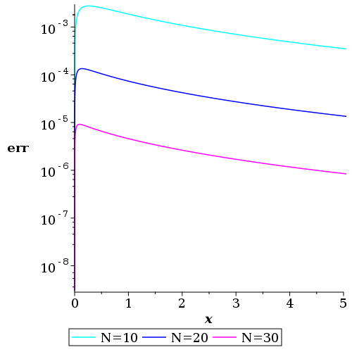
Figure 6: Comparison of values obtained via (34) and Majorana’s series for different numbers $N$ of terms.

We implemented this approach in Maple using the built-in solver for boundary value problems which could handle (33) without problems. We compared the results with solutions obtained via Majorana’s series, i. e. following Esposito [47], we entered a given number $N$ of terms into the integral defining $\mathcal{I}$ and performed a numerical integration. Fig. 6 shows on a logarithmic scale the absolute difference between our curve $\bigl{(}x(\sigma),u(\sigma)\bigr{)}$ and the curves computed via the series for different values of $N$. Obviously, our results are in an excellent agreement with the series solutions. The fact that all error curves have their maximum close to $x=0$ is easy to explain. As the expansion point of the series corresponds to $x=\infty$ (i. e. $t=1$), the series solutions become less accurate the closer one gets to $x=0$; at $x=0$ of course no error occurs, as this value is fixed by an initial condition. We did not make an extensive comparison of computation times. But plotting the series solution for $N=10$ over the interval $[0,5]$ required more than 10 times as much computation time than solving above boundary value problem demonstrating again the efficiency of our approach.

We mentioned already above that in the literature results are often presented only for rather small values of $x$, although the solution is defined for all non-negative real numbers. One exception is Amore et al. [52, Tbl. 3/4] who used a Padé–Hankel method and asymptotic expansions to present highly accurate values of the solution $u_{\infty}(x)$ and its first derivative $u_{\infty}^{\prime}(x)$ up to $x=400$.

$x$	$u_{\infty}(x)$	$u_{\infty}^{\prime}(x)$
$0$	$1$	$-1.58807101687867$
$10$	$0.0243142929534589$	$-0.00460288186903816$
$50$	$0.000632254782228818$	$-0.0000324989019998445$
$100$	$0.000100242568239745$	$-2.73935106365787\cdot 10^{-6}$
$150$	$0.0000326339644201454$	$-6.09139947257267\cdot 10^{-7}$
$200$	$0.0000145018034835377$	$-2.05753231409599\cdot 10^{-7}$
$250$	$7.67729076668264\cdot 10^{-6}$	$-8.78946798702223\cdot 10^{-8}$
$300$	$4.54857195240339\cdot 10^{-6}$	$-4.36594961733055\cdot 10^{-8}$
$350$	$2.91510210708972\cdot 10^{-6}$	$-2.40920109677041\cdot 10^{-8}$
$400$	$1.97973262954641\cdot 10^{-6}$	$-1.43668230750324\cdot 10^{-8}$

Table 5: Solution values $u_{\infty}(x)$ and derivative values $u_{\infty}^{\prime}(x)$ for large $x$.

Table 5 contains similar values obtained with our approach. For determining the values of $u_{\infty}^{\prime}(x)$, we must augment (34) by an equation for $u^{\prime}(\sigma)$, i. e. we must extend the parametrisation to the prolonged graph. By a straightforward application of the chain rule, one obtains

$$u^{\prime}(\sigma)=-3\cdot 144^{-1/3}v(\sigma)\exp{\bigl{(}-8\mathcal{I}(\sigma)\bigr{)}}\;.$$ (35)

To compile such a table, one must then determine for each $x$ the corresponding value of the parameter $\sigma$ via the solution of a nonlinear equation. Nevertheless, the complete computation of the values at the ten points contained in the table required only about 0.1 seconds. Amore et al. [52] claim that in their tables all digits are correct. Assuming that this is indeed the case, we can conclude that we obtained with minimal effort for each value of $x$ at least eight correct digits for $u_{\infty}(x)$ and seven correct digits for $u_{\infty}^{\prime}(x)$. Given the settings for the tolerances of our integrator and the use of hardware floats with only 10 digits, these results demonstrate again a very remarkable precision and efficiency of our approach. As large values of $x$ correspond to small values of $\sigma$ and thus to values of $t$ close to $1$, one may have to choose a smaller value of $\epsilon$ for very large values of $x$. The largest value appearing in above table, $x=400$, corresponds to $\sigma\approx 0.35$ and $t\approx 0.9789$. We chose for our numerical calculation the value $\epsilon=10^{-3}$ and thus used as right end of the approximated unstable manifold instead of the saddle point $(1,1)$ the point $(t_{1},v_{1})\approx(0.9978,1.001)$. For $x=400$, one may say that we are still sufficiently far away from this point, but for larger values of $x$ one should probably start working with a smaller value of $\epsilon$ which will increase the computation time, as the dynamics is very slow so close to a stationary point.

4.2.2 Other Solutions

So far, we only considered the particular solution $u_{\infty}$ (which has attracted the most attention in the literature). In Fig. 5 we presented the phase portrait for the Majorana transformed Thomas–Fermi equation. Using a slight modification (and simplification) of the above described backtransformation via the solution of an extended differential system, we can also obtain a “phase portrait” of the original Thomas–Fermi equation, i. e. we compute solutions for different values of the initial slope $u^{\prime}(0)$ keeping the initial condition $u(0)=1$. While the Majorana transformation itself is valid for any solution of the Thomas–Fermi equation, our ansatz for the back transformation has encoded this second initial condition (one could easily adapt to a different value $u(0)=c$ by multiplying (28) with the constant $c$). According to (24), each value of $u^{\prime}(0)$ corresponds uniquely to a value of $v(0)$. We now take the vector field $-Y_{\mathrm{red}}$ and use a parametrisation such that $s=0$ corresponds to $t=0$ (and thus also $x=0$). This leads to the following augmented initial value problem:

$$\begin{gathered}\frac{dt}{ds}=1-t^{2}v\;,\quad\frac{dv}{ds}=8(tv^{2}-1)\;,\quad\frac{d\mathcal{I}}{ds}=tv\;,\\[3.60004pt] t(0)=0\;,\quad v(0)=v_{0}\;,\quad\mathcal{I}(0)=0\;.\end{gathered}$$ (36)

Its solutions are then transformed into $x$- and $u$-coordinates via (34).

Fig. 7 shows that the solution $u_{\infty}$ vanishing at infinity acts as a kind of “separatrix”. The solutions above it, i. e. with an initial slope higher than $\omega$, pass through a minimum and then grow faster than exponentially (note the logarithmic scale). The solutions below it approach rapidly zero, reaching it at a finite value of $x$ (recall that the separatrix reaches zero at infinity). It turns out that around the critical value $\omega$, the trajectories are rather sensitive with respect to the initial slope. For some of the curves shown in Fig. 7, $u^{\prime}(0)$ differs only in the fifth or sixth digit. For the curves approaching zero, it is also non-trivial to determine the exact location of the zero, as here $v$ goes towards infinity. In our computations, we actually integrated only until some threshold like $10^{-8}$. Probably a “hybrid” approach using (36) only to get away from the singularity at $x=0$ and applying afterwards a standard integrator to the Thomas–Fermi equation would be a good alternative.

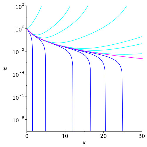
Figure 7: Solutions of the Thomas–Fermi equation with $u(0)=1$ and different $u^{\prime}(0)$ using a logarithmic scale for $u$. The curve in magenta shows $u_{\infty}$.

For solving concrete boundary value problems with boundary conditions of the form (4a) or (4c), resp., for given values of $a$ or $b$, resp., one can use an adapted version of a shooting method. Starting with an initial guess $v_{0}$ for the unknown value of $v(0)$ for the sought solution, one integrates the initial value problem (36) until a condition of the desired form is satisfied. However, in general, the condition will be satisfied at a wrong position $a^{*}$ or $b^{*}$, resp. Using a bisection, one modifies $v_{0}$ until one is sufficiently close to the actually prescribed values. As in both cases, Fig. 7 shows that there is a monotone relation between $v_{0}$ and $a^{*}$ or $b^{*}$, resp., it is always clear in which direction one has to change $v_{0}$. But for larger values of $a$ or $b$, one gets again into areas where very small changes in $v_{0}$ lead to significant changes in $a^{*}$ or $b^{*}$, resp. Despite this sensitivity, the approach worked in tests very well for $a\leq 27$ and $b\leq 30$.

5 Conclusions

The Lane–Emden and the Thomas–Fermi equation are prototypical examples for ordinary differential equations with singularities. Their singularities are determined by a specific value of the independent variable: $x=0$. Any initial or boundary value problem with conditions prescribed at $x=0$ cannot be tackled by standard methods and this concerns both theoretical and numerical studies.

The Lane–Emden equations fit into the framework of so-called Fuchsian equations (see e. g. [53]), i. e. equations of the form $Lu=f(x,u)$ where $L$ is a linear differential operator of Fuchsian type and where only the right hand side may contain nonlinear terms. For the theoretical treatment of such equations, some form of quasilinearisation is often fruitful, as it allows to use the far developed theory of the linear counterpart $Lu=\tilde{f}(x)$. For example, the existence and uniqueness proof for boundary value problems for (generalised) Lane–Emden equations given in [29] follows such strategy. For the numerical integration, [54] presents methods for first- and second-order systems of this particular form.

A key consequence of this special structure is the above mentioned location of the singularities depending only on $x$ which facilitates the design of specialised numerical methods. Therefore it is not surprising that so many different techniques have been proposed in the literature. Our approach is independent of such a special form, as one can see from our treatment of the Thomas–Fermi equation based on the reduced equation (23). The location of its singularities depends on $t$ and $v$ making an integration with standard numerical methods more difficult. By contrast, our approach can handle all forms of quasilinear problems.

In some computations related to the Thomas–Fermi equations, we encountered problems, for example when computing $u_{\infty}(x)$ for very large values of $x$ or when $u(x)$ approaches zero. In the first case, the reason lies in an often highly nonlinear relationship between the variable $t$ used in the reduced system and the variable $x$ where “microscopic” changes in $t$ may correspond to huge differences in $x$. In the second case, $u$ can approach $0$ only when $v$ tends towards infinity. In both cases, one could probably extend the applicability of our method by a rescaling of the reduced equation. For computing $u_{\infty}$ for large $x$, an alternative, semianalytic approach would consist of determining a higher order approximation of the unstable manifold close to the saddle point $(1,1)$ – in fact, the Majorana series is nothing else than such an approximation. This could lead to very accurate values even for extremely large values of $x$.

One may wonder why we used in the case of the Lane–Emden equations the shooting method for boundary value problems and not also a formulation as free boundary value problem as for the Thomas–Fermi equation. In both cases, one faces the problem that at one boundary one has to deal with a two-dimensional plane of stationary points and that the boundary conditions enforce that one end point of the solution trajectory lies on this plane. In the case of the Thomas–Fermi equation, we resolved this problem by moving a bit in the direction of the unstable eigenspace. This was possible, as this direction is the same for all points on the plane. In the case of the Lane–Emden equations, the direction of the unstable eigenspace depends on the value $u(0)$ and thus differs for different points on the plane. Probably one could adapt typical approaches to boundary value problems like collocation methods to this dependency. But as our emphasis in this paper lies on the use of standard methods, we refrained from studying this possibility in more details. Furthermore, the simple shooting method works very well and reliable for this class of problems.

Data

All computations presented in this article (and a few more) were performed within Maple worksheets. These are freely available at Zenodo using the DOI https://doi.org/10.5281/zenodo.10064926.

References

- [1] R. Emden, Gaskugeln, Teubner, Leipzig, 1907.
- [2] H. Davis, Introduction to Nonlinear Differential and Integral Equations, Dover, New York, 1962.
- [3] C. Hansen, S. Kawaler, V. Trimble, Stellar Interiors, 2nd Edition, Astronomy and Astrophysics Library, Springer-Verlag, New York, 2004.
- [4] G. Horedt, Polytropes — Applications in Astrophysics and Related Fields, Astrophysics and Space Science Library 306, Kluwer, New York, 2004.
- [5] L. Thomas, The calculation of atomic fields, Proc. Cambr. Philos. Soc. 23 (1927) 542–548.
- [6] E. Fermi, Eine statistische Methode zur Bestimmung einiger Eigenschaften des Atoms und ihre Anwendung auf die Theorie des periodischen Systems der Elemente, Z. Phys. 48 (1928) 73–79.
- [7] E. Di Grezia, S. Esposito, Fermi, Majorana and the statistical model of atoms, Found. Phys. 34 (2004) 1431–1450.
- [8] N. March, The Thomas–Fermi approximation in quantum mechanics, Adv. Phys. 6 (1957) 1–101.
- [9] I. Torrens, Interatomic Potentials, Academic Press, New York, 1972.
- [10] E. Hille, On the Thomas–Fermi equation, Proc. Natl. Acad. Sci. USA 62 (1969) 7–10.
- [11] E. Hille, Some aspects of the Thomas–Fermi equation, J. Anal. Math. 23 (1970) 147–170.
- [12] G. Horedt, Seven-digit tables of Lane–Emden functions, Astrophys. Space Sci. 126 (1986) 357–408.
- [13] R. Russell, L. Shampine, Numerical methods for singular boundary value problems, SIAM J. Num. Anal. 12 (1975) 13–36.
- [14] V. Arnold, Geometrical Methods in the Theory of Ordinary Differential Equations, Edition, Grundlehren der mathematischen Wissenschaften 250, Springer-Verlag, New York, 1988.
- [15] A. Remizov, Multidimensional Poincaré construction and singularities of lifted fields for implicit differential equations, J. Math. Sci. 151 (2008) 3561–3602.
- [16] W. Seiler, Singularities of implicit differential equations and static bifurcations, in: V. Gerdt, W. Koepf, E. Mayr, E. Vorozhtsov (Eds.), Computer Algebra in Scientific Computing — CASC 2013, Lecture Notes in Computer Science 8136, Springer-Verlag, Cham, 2013, pp. 355–368.
- [17] W. Seiler, M. Seiß, Singular initial value problems for scalar quasi-linear ordinary differential equations, J. Diff. Eq. 281 (2021) 258–288.
- [18] E. Braun, W. Seiler, M. Seiß, On the numerical analysis and visualisation of implicit ordinary differential equations, Math. Comput. Sci. 14 (2020) 281–293.
- [19] W. Seiler, Involution — The Formal Theory of Differential Equations and its Applications in Computer Algebra, Algorithms and Computation in Mathematics 24, Springer-Verlag, Berlin, 2010.
- [20] U. Kant, W. Seiler, Singularities in the geometric theory of differential equations, in: W. Feng, Z. Feng, M. Grasselli, X. Lu, S. Siegmund, J. Voigt (Eds.), Dynamical Systems, Differential Equations and Applications (Proc. 8th AIMS Conference, Dresden 2010), Vol. 2, AIMS, 2012, pp. 784–793.
- [21] M. Lange-Hegermann, D. Robertz, W. Seiler, M. Seiß, Singularities of algebraic differential equations, Adv. Appl. Math. 131 (2021) 102266.
- [22] W. Beyn, W. Kleß, Numerical Taylor expansion of invariant manifolds in large dynamical systems, Numer. Math. 80 (1998) 1–38.
- [23] T. Eirola, J. von Pfaler, Taylor expansion for invariant manifolds, Numer. Math. 80 (1998) 1–38.
- [24] J. Liang, A singular initial value problem and self-similar solutions of a nonlinear dissipative wave equation, J. Diff. Eqs. 246 (2009) 819–844.
- [25] J. Sijbrand, Properties of center manifolds, Trans. AMS 289 (1985) 431–469.
- [26] W. Seiler, M. Seiß, Singular initial value problems for quasi-linear systems of ordinary differential equations, in preparation (2022).
- [27] G. Vainikko, A smooth solution to a linear system of singular ODEs, Zeitsch. Analysis Anwend. 32 (2013) 349–370.
- [28] G. Vainikko, A smooth solution to a nonlinear system of singular ODEs, in: T. Simos, G. Psihoyios, C. Tsitouras (Eds.), Proc. 11th Int. Conf. Numerical Analysis and Applied Mathematics (ICNAAM 2013), AIP Conf. Proc. 1558, Amer. Inst. Physics, 2013, pp. 758–761.
- [29] M. Chawla, P. Shivakumar, On the existence of solutions of a class of singular nonlinear two-point boundary value problems, J. Comp. Appl. Math. 19 (1987) 379–388.
- [30] K. Parand, M. Deghan, A. Rezaei, S. Ghaderi, An approximation algorithm for the solution of the nonlinear Lane–Emden type equations arising in astrophysics using Hermite functions collocation method, Comp. Phys. Comm. 181 (2010) 1096–1108.
- [31] R. Aris, Introduction to the Analysis of Chemical Reactors, International Series in the Physical and Chemical Engineering Sciences, Prentice-Hall, Englewood Cliffs, 1965.
- [32] D. Flockerzi, K. Sundmacher, On coupled Lane–Emden equations arising in dusty fluid models, J. Phys. Conf. Ser. 268 (2011) 012006.
- [33] T. Praveen, P. Valencia, L. Rajendran, Theoretical analysis of intrinsic reaction kinetics and the behavior of immobilized enzymes system for steady-state conditions, Biochem. Eng. J. 91 (2014) 129–139.
- [34] A. Ananthaswamy, R. Shanthakumari, M. Subha, Simple analytical expressions of the non-linear reaction diffusion process in an immobilized biocatalyst particle using the new homotopy perturbation method, Rev. Bioinform. Biometr. 3 (2014) 22–28.
- [35] L. Shampine, J. Kierzenka, A BVP solver based on residual control and the MATLAB PSE, ACM Trans. Math. Softw. 27 (2001) 299–316.
- [36] L. Shampine, J. Kierzenka, A BVP solver that controls residual and error, J. Numer. Anal. Ind. Appl. Math. 3 (2008) 27–41.
- [37] R. Skeel, M. Berzins, A method for the spatial discretization of parabolic equations in one space variable, SIAM J. Sci. Stat. Comp. 11 (1990) 1–32.
- [38] S. Lin, Oxygen diffusion in a spherical cell with nonlinear oxygen uptake kinetics, J. Theor. Biol. 60 (1976) 449–457.
- [39] D. McElwain, A re-examination of oxygen diffusion in a spherical cell with Michaelis–Menten oxygen uptake kinetics, J. Theor. Biol. 71 (1978) 255–263.
- [40] P. Hiltmann, P. Lory, On oxygen diffusion in spherical cell with Michaelis–Menten uptake kinetics, Bull. Math. Biol. 45 (1983) 661–664.
- [41] S. Khury, A. Sayfy, A novel approach for the solution of a class of singular boundary value problems arising in physiology, Math. Comp. Modell. 52 (2010) 626–636.
- [42] H. Çağlar, N. Çağlar, M. Özer, B-spline solution of non-linear singular boundary value problems arising in physiology, Chaos Solit. Fract. 39 (2009) 1232–1237.
- [43] F. de Hoog, R. Weiss, Difference methods for boundary value problems with a singularity of the first kind, SIAM J. Numer. Anal. 13 (1976) 775–813.
- [44] M. Campesi, N. Mariani, S. Bressa, M. Pramparo, B. Barbero, L. Cadús, G. Baretto, O. Martínez, Kinetic study of the combustion of ethanol and ethyl acetate mixtures over a MnCu catalyst, Fuel Proc. Technol. 103 (2012) 84–90.
- [45] V. Meena, T. Praveen, L. Rajendran, Mathematical modeling and analysis of the molar concentrations of ethanol, acetaldehyde and ethyl acetate inside the catalyst particle, Kinet. Catal. 57 (2016) 125–134.
- [46] S. Bressa, N. Mariani, N. Ardiaca, G. Mazza, O. Martínez, G. Barreto, An algorithm for evaluating reaction rates of catalytic reaction networks with strong diffusion limitations, Comp. Chem. Eng. 25 (2001) 1185–1198.
- [47] S. Esposito, Majorana solution of the Thomas–Fermi equation, Amer. J. Phys. 70 (2002) 852–856.
- [48] S. Esposito, Majorana transformation for differential equations, Int. J. Theor. Phys. 41 (2002) 2417–2426.
- [49] A. Mambriani, Su un teorema relativo alle equazioni differenziali ordinarie del ordine, Rend. Accad. Naz. Lincei, Cl. Sci. Fis. Mat. Nat. (Ser. VI) 9 (1929) 620–629.
- [50] K. Parand, M. Delkosh, Accurate solution of the Thomas–Fermi equation using the fractional order of rational Chebyshev functions, J. Comp. Appl. Math. 317 (2017) 624–642.
- [51] F. Fernández, J. Garcia, On the Majorana solution to the Thomas–Fermi equation, arXiv:2105.02686 (2021).
- [52] P. Amore, J. Boyd, F. Fernández, Accurate calculation of the solutions to the Thomas–Fermi equations, Appl. Math. Comp. 232 (2014) 929–943.
- [53] S. Kichenassamy, Fuchsian Reduction, Progress in Nonlinear Differential Equations and Their Applications 71, Birkhäuser, Boston, 2007.
- [54] O. Koch, P. Kofler, E. Weinmüller, Initial value problems for systems of ordinary first and second order differential equations with a singularity of the first kind, Analysis 21 (2001) 373–389.