Robust Inference for Federated Meta-Learning

Abstract

Synthesizing information from multiple data sources is critical to ensure knowledge generalizability. Integrative analysis of multi-source data is challenging due to the heterogeneity across sources and data-sharing constraints due to privacy concerns. In this paper, we consider a general robust inference framework for federated meta-learning of data from multiple sites, enabling statistical inference for the prevailing model, defined as the one matching the majority of the sites. Statistical inference for the prevailing model is challenging since it requires a data-adaptive mechanism to select eligible sites and subsequently account for the selection uncertainty. We propose a novel sampling method to address the additional variation arising from the selection. Our devised CI construction does not require sites to share individual-level data and is shown to be valid without requiring the selection of eligible sites to be error-free. The proposed robust inference for federated meta-learning (RIFL) methodology is broadly applicable and illustrated with three inference problems: aggregation of parametric models, high-dimensional prediction models, and inference for average treatment effects. We use RIFL to perform federated learning of mortality risk for patients hospitalized with COVID-19 using real-world EHR data from 16 healthcare centers representing 275 hospitals across four countries.

1 Introduction

Crowdsourcing, or the process of aggregating crowd wisdom to solve problems, is a useful community-based method to improve decision-making in disciplines ranging from education (Heffernan and Heffernan, 2014) to public health (Han et al., 2018; Wang et al., 2020). Compared to traditional expert-driven solutions made by a single group, incorporating the opinions of multiple diverse groups can improve the quality of the final decision (Surowiecki, 2005). In health research, crowdsourcing has led to the discovery of new drugs during pandemics (Chodera et al., 2020), the design of patient-centered mammography reports (Short et al., 2017), and the development of machine learning algorithms to classify tumors for radiation therapy (Mak et al., 2019).

Underlying the phenomenon of the “wisdom of the crowds” is the statistical and philosophical notion that learning from multiple data sources is desirable. Incorporating information from diverse data sources can increase the generalizability and transportability of findings compared to learning from a single data source. Findings from a single data source may not be generalizable to a new target population of interest due to poor data quality or heterogeneity in the underlying data generating processes.

Integrative analysis of data from multiple sources can be a valuable alternative to using a single data source alone. However, directly pooling multiple data sources into a single dataset for analysis is often unsatisfactory or even infeasible. Heterogeneity between different data sources can severely bias predictions or inferences made by such a pooled analysis strategy (Leek et al., 2010; Ling et al., 2022). As an alternative to pooled analysis, meta-analysis has frequently synthesized information from multiple studies. Standard meta-analysis methods aggregate quantitative summary of evidence from multiple studies. Variations of meta-analysis, such as random effects meta-analysis, have been adopted to explore between-study heterogeneity, potential biases such as publication bias, and small-study effects. However, most existing meta-analysis tools that account for heterogeneity require strong modeling assumptions and do not consider the validity of inference when data from certain sites have substantially different distributions from other sites.

Another challenge of particular importance is the issue of data privacy pertaining to biomedical studies. Regulations in the United States, such as the Health Insurance Portability and Accountability Act (HIPAA) Privacy Rule, and those in the European Union, such as the General Data Protection Regulation (GDPR) and the European Medicines Agency (EMA) Privacy Statement, protect the personal information of patients and preclude the transfer of patient-level data between sites. These regulations make the promise of integrative data analysis more difficult to attain, highlighting the need for federated integrative analysis methods that do not require sharing of individual-level data.

When cross-study heterogeneity is substantial and outliers exist, a desirable strategy of integrative analysis is to identify a prevailing model to achieve consensus learning. The prevailing model is defined as the model satisfied by the majority of the sites. Identifying the prevailing model can be intuitively achieved via the majority rule (Sorkin et al., 1998; Kerr et al., 2004; Hastie and Kameda, 2005), which chooses the alternative that more than half of individuals agree upon. The majority rule is widespread in modern liberal democracies and is deployed in various streams of research. For example, genomics data is usually separated into batches, but heterogeneity across batches can lead to undesirable variation in the data (Leek et al., 2010; Ling et al., 2022). This setting aims to identify batches that show low levels of concordance with the majority of the batches and adjust for such differences in downstream analyses (Trippa et al., 2015). As another example, in the design of clinical trials, it is often infeasible or unethical to enroll patients in the control arm. In such cases, it is possible to use data from historical trials or observational studies to construct an external control arm (Jahanshahi et al., 2021; Ventz et al., 2019; Davi et al., 2020). However, when many such historical data sources exist, it is crucial to carefully select data sources that show high levels of similarity with the majority of the other data sources. The last example is Mendelian Randomization, where multiple genetic markers are used as instrumental variables (IVs) to account for potential unmeasured confounders. Every single IV will have its causal effect estimator, and the goal is to identify the causal effect matching the majority of the estimated effects (Burgess et al., 2017; Bowden et al., 2016; Kang et al., 2016).

Without prior knowledge of the prevailing model, it is critical to employ data-adaptive approaches to select appropriate sites for inferring the prevailing model. In addition, confidence intervals (CIs) for the target parameter of the prevailing model need to appropriately adjust for the site selection variability. Most existing statistical inference methods rely on perfectly separating eligible and ineligible sites, which may be unrealistic for practical applications. There is a paucity of statistical inference methods for the prevailing model that can achieve efficient and robust inference while being applicable to a broad set of scenarios without restrictive assumptions such as a perfect separation.

In this paper, we fill this gap by developing a broad theoretically justified framework for making robust inferences for federated meta-learning (RIFL) of an unknown prevailing model using multi-source data. The RIFL method selects the eligible sites to infer the prevailing model by assessing dissimilarities between sites with regard to the parameter of interest. We employ a novel resampling method to construct uniformly valid CIs. The RIFL inference method is robust to the errors in separating the sites belonging to the majority group and the remaining sites; see Theorem 2. We also show in Theorem 3 that our proposed sampling CI can be as short as the oracle CI with the prior knowledge of the eligible sites. Our general sampling algorithm is privacy-preserving in that it is implemented using site-specific summary statistics and without requiring sharing individual-level data across different sites. Our proposed RIFL methodology is demonstrated with three inference problems: aggregation of low-dimensional parametric models, construction of high-dimensional prediction models, and inference for the average treatment effect (ATE).

To the best of our knowledge, our proposed RIFL method is the first CI guaranteeing uniform coverage of the prevailing model under the majority rule. We have further compared via simulation studies with three other inference procedures that can potentially be used under the majority rule, including the majority voting estimator, the median estimator (e.g., Bowden et al., 2016), and the m-out-of-n bootstrap (e.g., Chakraborty et al., 2013; Andrews, 2000). Numerical results demonstrate that these three CIs fail to achieve the desired coverage property, while our RIFL method leads to a uniformly valid CI. We provide the reasoning for under-coverage for these existing methods in Sections 2.3 and 2.4.

1.1 Related literature

The RIFL method is related to multiple streams of literature, including post-selection inference, mendelian randomization, integrative analysis of multi-source data, transfer learning, and federated learning. We next detail how RIFL differs from the existing literature and highlight its contributions.

A wide range of novel methods and theories have been established to address the post-selection inference problem (e.g., Berk et al., 2013; Lee et al., 2016; Leeb and Pötscher, 2005; Zhang and Zhang, 2014; Javanmard and Montanari, 2014; van de Geer et al., 2014; Chernozhukov et al., 2015; Belloni et al., 2014; Cai and Guo, 2017; Xie and Wang, 2022). However, most post-selection inference literature focuses on inferences after selecting a small number of important variables under high-dimensional regression models. The selection problem under the RIFL framework is fundamentally different: the selection error comes from comparing different sites, and there is no outcome variable to supervise the selection process. Additionally, RIFL only requires the majority rule, while the variable selection methods typically require a small proportion of variables to affect the outcome.

In Mendelian Randomization, various methods have been developed to leverage the majority rule and make inferences for the one-dimensional causal effect (Bowden et al., 2016; Windmeijer et al., 2019; Kang et al., 2016; Guo et al., 2018; Windmeijer et al., 2021). A recent work by Guo (2021) demonstrated the post-selection problem due to IV selection errors. However, the uniformly valid inference method in Guo (2021) relies on searching the one-dimensional space of the causal effect and cannot be easily generalized to multivariate settings, not to mention high-dimensional settings. In contrast, RIFL is distinct from the existing searching method and is useful in addressing a much broader collection of post-selection problems as detailed in Section 5.

The integrative analysis of multi-source data has been investigated in different directions. Wang et al. (2021) studied the data fusion problem with robustness to biased sources. The identification condition in Wang et al. (2021) differs from the majority rule, and the validity of their proposal requires correctly identifying unbiased sources. Maity et al. (2022) studied meta-analysis in high-dimensional settings where the data sources are similar but non-identical and require the majority rule to be satisfied as well as a large separation between majority and outlier sources to perfectly identify eligible sites. In contrast, the RIFL CI is valid without requiring the selection step to perfectly identify eligible sites. Meinshausen and Bühlmann (2015); Bühlmann and Meinshausen (2015); Rothenhäusler et al. (2016); Guo (2020) made inference for the maximin effect, which is defined as a robust prediction model across heterogeneous datasets. Cai et al. (2021b); Liu et al. (2021); Zhao et al. (2016) imposed certain similar structures across different sources and made inferences for the shared component of regression models. Peters et al. (2016); Arjovsky et al. (2019) studied the multi-source data problem and identified the causal effect by invariance principles. Unlike existing methods, the RIFL framework only assumes that a majority of the sites have similar models but allows non-eligible sites to differ arbitrarily from the majority group.

RIFL relates to the existing literature on federated learning and transfer learning. Privacy-preserving and communication-efficient algorithms have been recently developed to learn from multiple sources of electronic health records (EHR) (Rasmy et al., 2018; Tong et al., 2022) and multiple sources of diverse genetic data (Kraft et al., 2009; Keys et al., 2020). Federated regression and predictive modeling (Chen et al., 2006; Li et al., 2013; Chen and Xie, 2014; Lee et al., 2017; Lian and Fan, 2017; Wang et al., 2019; Duan et al., 2020) and causal modeling (Xiong et al., 2021; Vo et al., 2021; Han et al., 2021) have been developed. However, none of these federated learning methods study inference for the prevailing model when some sites may not be valid, which is the main focus of RIFL. The RIFL framework also differs from the recently developed transfer learning algorithms (e.g., Li et al., 2020; Tian and Feng, 2022; Han et al., 2021). These algorithms require pre-specification of an anchor model to which the models obtained from source data sets can be compared. In contrast, RIFL targets a more challenging scenario: we do not assume the availability of such an anchor model but leverage the majority rule to identify the unknown prevailing model.

1.2 Paper organization and notations

The paper proceeds as follows. Section 2 describes the multi-source data setting and highlights the challenge of inferring the prevailing model. Section 3 proposes the RIFL methodology, and Section 4 establishes its related theory. In Section 5, we illustrate our proposal in three applications. In Section 6, we provide extensive simulation results comparing our method to existing methods. Section 7 illustrates our method using real-world international EHR data from 16 participating healthcare centers representing 275 hospitals across four countries as part of the multi-institutional Consortium for the Clinical Characterization of COVID-19 by EHR (4CE) (Brat et al., 2020).

We introduce the notations used throughout the paper. For a set $A$, $|A|$ denotes the cardinality of the set. For a vector $x$, we define its $\ell_{q}$ norm as $\|x\|_{q}=\left(\sum_{l=1}^{p}|x_{l}|^{q}\right)^{\frac{1}{q}}$ for $q\geq 0$ with $\|x\|_{0}=\left|\{1\leq l\leq p:x_{l}\neq 0\}\right|$ and $\|x\|_{\infty}=\max_{1\leq l\leq p}|x_{l}|$. For a matrix $X$, $X_{i,\cdot}$ and $X_{\cdot,j}$ denote its $i$-th row and $j$-th column, respectively. For two positive sequences $a_{n}$ and $b_{n}$, $a_{n}\ll b_{n}$ if $\limsup_{n\rightarrow\infty}{a_{n}}/{b_{n}}=0$. For a matrix $A$, we use $\|A\|_{F}$, $\|A\|_{2}$ and $\|A\|_{\infty}$ to denote its Frobenius norm, spectral norm, and element-wise maximum norm, respectively.

2 Formulation and Statistical Inference Challenges

2.1 Model assumptions and overview of RIFL

Throughout the paper, we consider that we have access to $L$ independent training data sets drawn from $L$ source populations. For $1\leq l\leq L$, we use $\mathbb{P}^{(l)}$ to denote the distribution of the $l$-th source population and use $\theta^{(l)}=\theta(\mathbb{P}^{(l)})\in\mathbb{R}^{d}$ to denote the associated model parameter. For any $\theta\in\mathbb{R}^{d}$, we define the index set $\mathcal{V}(\theta)\subset\{1,\cdots,L\}$ as

$$\mathcal{V}(\theta)\coloneqq\{1\leq l\leq L:\theta^{(l)}=\theta\},$$ (1)

which contains the indexes of all sites having the same model parameter as $\theta.$ We now introduce the majority rule.

Assumption 1 (Majority Rule)

There exists $\theta^{*}\in\mathbb{R}^{d}$ such that $\left|\mathcal{V}(\theta^{*})\right|>L/2.$

We shall refer to $\theta^{*}$ as the prevailing model that matches with more than half of $\{\theta^{(l)}\}_{1\leq l\leq L}$, and the corresponding index set $\mathcal{V}(\theta^{*})$ as the prevailing set. Our goal is to construct a confidence region for a low dimensional functional of $\theta^{*}$, denoted as $\beta^{*}={g}(\theta^{*})\in\mathbb{R}^{q}$, for some $q\geq 1,$ where ${g}(\cdot)\in\mathbb{R}^{q}$ is a prespecified low-dimensional transformation. Examples of $\beta^{*}={g}(\theta^{*})$ include

1. Single coefficient or sub-vector: $\beta^{*}=\theta^{*}_{j}$ for $1\leq j\leq d$ or $\beta^{*}=\theta^{*}_{G}$ with $G\subset\{1,\cdots,d\}$;

2. Linear transformation: $\beta^{*}=x^{\intercal}\theta^{*}$ for any $x\in\mathbb{R}^{d}$;

3. Quadratic form: $\beta^{*}=\|\theta^{*}\|_{2}^{2}$.

For notational ease, we focus on $q=1$ primarily and discuss the extension to the setting with $q\geq 2$ in Section 3.2.

If the prevailing set $\mathcal{V}(\theta^{*})$ were known, standard meta and federated learning methods could be used to make inferences about $\theta^{*}$ using data from sites belonging to $\mathcal{V}(\theta^{*}).$ However, as highlighted in Section 2.3, inference for $\theta^{*}$ without prior knowledge of $\mathcal{V}(\theta^{*})$ except for the majority rule is substantially more challenging due to the need to estimate $\mathcal{V}(\theta^{*})$. Our proposed RIFL procedure involves several key steps: (i) for $l=1,...,L$, construct local estimates of $\theta^{(l)}$ and $\beta^{(l)}=g(\theta^{(l)})$, denoted by $\widehat{\theta}^{(l)}$ and $\widehat{\beta}^{(l)}$, respectively; (ii) for $1\leq l<k\leq L$, estimate pairwise dissimilarity measure $\mathcal{D}_{l,k}=D(\theta^{(l)},\theta^{(k)})$ and ${\mathcal{L}}_{l,k}=\beta^{(l)}-\beta^{(k)}$ as $\widehat{\mathcal{D}}_{l,k}$ and $\widehat{\mathcal{L}}_{l,k}$ along with their standard errors $\widehat{\mbox{SE}}(\widehat{\mathcal{D}}_{l,k})$ and $\widehat{\mbox{SE}}(\widehat{\mathcal{L}}_{l,k})$; (iii) construct a robust estimate for the prevailing set $\mathcal{V}(\theta^{*})$; (iv) derive robust resampling-based confidence set for $\beta^{*}$ accounting for post-selection uncertainty. The construction of $\widehat{\theta}^{(l)}$ and $\widehat{\beta}^{(l)}$ follows standard procedures for the specific problems of interest. We next detail (ii) the construction of the dissimilarity measures and (iii) the prevailing set estimator. The most challenging step of RIFL is the resampling-based inference, which is described in Section 3.

2.2 Dissimilarity measures

A critical step of applying the majority rule is to evaluate the (dis)similarity between any pair of parameters $\theta^{(l)}$ and $\theta^{(k)}$ for $1\leq l,k\leq L.$ We form two sets of dissimilarity measures, the local dissimilarity between $\beta^{(l)}$ and $\beta^{(k)}$, ${\mathcal{L}}_{l,k}=\beta^{(l)}-\beta^{(k)}$, and a global dissimilarity $\mathcal{D}_{l,k}=\mathcal{D}(\theta^{(l)},\theta^{(k)})=\|\theta^{(l)}-\theta^{(k)}\|_{2}^{2}$. Although other vector norms can be considered for $\mathcal{D}(\cdot,\cdot)$, we focus on the quadratic norm due to its smoothness and ease of inference, especially in the high-dimensional setting.

We assume that $\{\widehat{\beta}^{(l)},\widehat{\sigma}_{l}\}_{1\leq l\leq L}$ satisfy

$$\frac{1}{{\sigma}_{l}}(\widehat{\beta}^{(l)}-\beta^{(l)})\overset{d}{\to}N(0,1)\quad\text{and}\quad\frac{\widehat{\sigma}_{l}}{{\sigma}_{l}}\overset{p}{\to}1,$$ (2)

with $\sigma_{l}$ denoting the standard error of $\widehat{\beta}^{(l)}.$ In the low-dimensional setting, most existing estimators satisfy (2) under standard regularity conditions. In the high-dimensional setting, various asymptotically normal de-biased estimators have recently been proposed and shown to satisfy (2); see more discussions at the end of Section 5.2.

Let $\widehat{\mathcal{L}}_{l,k}=\widehat{\beta}^{(l)}-\widehat{\beta}^{(k)}$ and $\widehat{\mathcal{D}}_{l,k}$ be the point estimators for ${\mathcal{L}}_{l,k}$ and $\mathcal{D}_{l,k}$, respectively. We estimate their standard errors as $\widehat{\mbox{SE}}(\widehat{\mathcal{L}}_{l,k})=\sqrt{\widehat{\sigma}_{l}^{2}+\widehat{\sigma}_{k}^{2}}$ and $\widehat{\mbox{SE}}(\widehat{\mathcal{D}}_{l,k})$, with $\widehat{\sigma}_{l}^{2}$ denoting the estimated variance of $\widehat{\beta}^{(l)}$. For the global dissimilarity measure, we assume that $\widehat{\mathcal{D}}_{l,k}$ and $\widehat{\rm SE}(\widehat{\mathcal{D}}_{l,k})$ satisfy

$$\limsup_{n\rightarrow\infty}{\mathbf{P}}\left({\left|\widehat{\mathcal{D}}_{l,k}-{\mathcal{D}}_{l,k}\right|}/{\widehat{\rm SE}(\widehat{\mathcal{D}}_{l,k})}\geq z_{\alpha}\right)\leq\alpha\quad\text{for}\quad 0<\alpha<1,$$ (3)

where $z_{\alpha}$ denotes the $\alpha$ upper quantile of a standard normal distribution. Although $\widehat{\mathcal{D}}_{l,k}$ can be constructed as $\|\widehat{\theta}^{(l)}-\widehat{\theta}^{(k)}\|_{2}^{2}$ in the low-dimensional setting, deriving $\{\widehat{\mathcal{D}}_{l,k},\widehat{\rm SE}(\widehat{\mathcal{D}}_{l,k})\}$ that satisfies (3) is much more challenging in the high-dimensional setting due to the inherent bias in regularized estimators. In Sections 5.1 and 5.2, we demonstrate that our proposed estimators of ${\mathcal{D}}_{l,k}$ satisfy (3) for a broad class of applications in both low and high dimensions.

Based on both sets of dissimilarity measures, we determine the concordance between sites $k$ and $l$ with respect to inference for $\beta^{*}=g(\theta^{*})$ based on the following test statistic

$$\widehat{S}_{l,k}\coloneqq\max\left\{\left|\widehat{\mathcal{D}}_{l,k}/{\widehat{\rm SE}(\widehat{\mathcal{D}}_{l,k})}\right|,\left|\widehat{{\mathcal{L}}}_{l,k}/{\widehat{\rm SE}(\widehat{{\mathcal{L}}}_{l,k})}\right|\right\}.$$ (4)

For $1\leq l<k\leq L$, we can then implement the following significance test of whether the $k$-th and $l$-th sites share the same parameters,

$$\widehat{H}_{l,k}={\bf 1}\left(\widehat{S}_{l,k}\leq z_{0.05/[2L(L-1)]}\right),$$ (5)

where $0.05$ is a pre-selected significance level for testing the similarity among different sites and $z_{0.05/[2L(L-1)]}$ denotes the $0.05/[2L(L-1)]$ upper quantile of the standard normal distribution. The statistic $\widehat{S}_{l,k}$ measures the level of evidence that the two sites differ from each other based on observed data. The binary decision $\widehat{H}_{l,k}$ in (5) essentially estimates $H_{l,k}={\bf 1}\{\theta^{(l)}=\theta^{(k)}\}.$ We specify the threshold as $z_{0.05/[2L(L-1)]}$ to adjust for the multiplicity of hypothesis testing. Since the matrix $H$ is symmetric and $H_{l,l}=1$, we construct an estimate for the full voting matrix $\widehat{H}=[\widehat{H}_{l,k}]_{l=1,...,L}^{k=1,...,L}$ by setting $\widehat{H}_{k,l}=\widehat{H}_{l,k}$ and $\widehat{H}_{l,l}=1$. The estimated voting matrix $\widehat{H}$ summarizes all cross-site similarities, which is then used to estimate the prevailing set.

Remark 1 (Univariate case)

For the special setting with a univariate $\theta^{*},$ we may simplify the construction of the test statistics in (4) and the vote in (5) as

$$\widehat{H}_{l,k}={\bf 1}\left(\widehat{S}_{l,k}\leq z_{0.05/[L(L-1)]}\right)\quad\text{with}\quad\widehat{S}_{l,k}=\left|\widehat{{\mathcal{L}}}_{l,k}/{\widehat{\rm SE}(\widehat{{\mathcal{L}}}_{l,k})}\right|\quad\text{for}\quad 1\leq l<k\leq L.$$ (6)

2.3 Prevailing set estimation and post-selection problem

In the following, we construct two estimators of the prevailing set $\mathcal{V}(\theta^{*})$, which are used to make inference for $\beta^{*}.$ We construct the first estimator as

$$\widetilde{\mathcal{V}}\coloneqq\{1\leq l\leq L:\|\widehat{H}_{l,\cdot}\|_{0}>L/2\}.$$ (7)

The set $\widetilde{\mathcal{V}}$ contains all sites receiving ‘majority votes’. The second estimator is constructed by utilizing the maximum clique from graph theory (Carraghan and Pardalos, 1990). Specifically, we define the graph $\mathcal{G}([L],\widehat{H})$ with vertices $[L]\coloneqq\{1,2,\cdots,L\}$ and the adjacency matrix $\widehat{H}$ with $\widehat{H}_{l,k}=1$ and $\widehat{H}_{l,k}=0$ denoting that the $l$-th and $k$-th vertexes are connected and disconnected, respectively. The maximum clique of the graph $\mathcal{G}([L],\widehat{H})$ is defined as the largest fully connected sub-graph. We use the term maximum clique set to denote the corresponding vertex set in the maximum clique, denoted as $\mathcal{MC}([L],\widehat{H}).$ We construct $\widehat{\mathcal{V}}$ by identifying the maximum clique set of $\mathcal{G}([L],\widehat{H})$, that is,

$$\widehat{\mathcal{V}}\coloneqq\mathcal{MC}([L],\widehat{H}).$$ (8)

If the majority rule holds, the prevailing set $\mathcal{V}(\theta^{*})$ is the maximum clique set of $\mathcal{G}([L],H)$, that is, $\mathcal{V}(\theta^{*})=\mathcal{MC}([L],{H})$. If $\widehat{H}$ is a sufficiently accurate estimator of $H$, both set estimators $\widetilde{\mathcal{V}}$ and $\widehat{\mathcal{V}}$ exactly recover the prevailing set $\mathcal{V}(\theta^{*}).$ However, since $\widehat{H}$ might be different from the true $H$ due to the limited sample size in practice, $\widetilde{\mathcal{V}}$ and $\widehat{\mathcal{V}}$ may be different from $\mathcal{V}(\theta^{*})$. When the maximum clique set has the cardinality above $L/2,$ we have $\widehat{\mathcal{V}}\subset\widetilde{\mathcal{V}}$, that is, $\widehat{\mathcal{V}}$ may be a more restrictive set estimator than $\widetilde{\mathcal{V}}.$ We illustrate the definitions of $\widetilde{\mathcal{V}}$ in (7) and $\widehat{\mathcal{V}}$ in (8) in Figure 1.

Figure 1: The graph $\mathcal{G}([L],\widehat{H})$ with $L=6.$ $\widetilde{\mathcal{V}}=\{1,2,3,4,5\}$ and $\widehat{\mathcal{V}}=\{1,2,3,5\}$.

In the following, we demonstrate the subsequent analysis after obtaining $\widehat{\mathcal{V}}.$ The argument is easily extended to the estimated set $\widetilde{\mathcal{V}}.$ One may aggregate $\{\widehat{\beta}^{(l)},\widehat{\sigma}_{l}\}_{l\in\widehat{\mathcal{V}}}$ to estimate $\beta^{*}$ as the following inverse variance weighted estimator,

$$\widehat{\beta}^{*}=\frac{\sum_{l\in\widehat{\mathcal{V}}}{\widehat{\beta}^{(l)}}/{\widehat{\sigma}_{l}^{2}}}{\sum_{l\in\widehat{\mathcal{V}}}1/{\widehat{\sigma}_{l}^{2}}}.$$ (9)

A naive $1-\alpha$ confidence interval for $\beta^{*}$ can be constructed as

$${\rm CI}_{\rm post}=\left(\widehat{\beta}^{*}-z_{\alpha/2}\frac{1}{\sqrt{\sum_{l\in\widehat{\mathcal{V}}}1/{\widehat{\sigma}_{l}^{2}}}},\widehat{\beta}^{*}+z_{\alpha/2}\frac{1}{\sqrt{\sum_{l\in\widehat{\mathcal{V}}}1/{\widehat{\sigma}_{l}^{2}}}}\right),$$ (10)

where $z_{\alpha/2}$ denotes the $\alpha/2$ upper quantile of the standard normal distribution.

Unfortunately, similar to other settings in the ‘post-selection’ literature, such naive construction can lead to bias in the point estimation and under-coverage in the confidence interval due to ignoring the variability in the selection of $\widehat{\mathcal{V}}$. We illustrate the post-selection problem of the naive confidence interval in (10) with the following example.

Example 1

We construct the confidence interval for a target population’s average treatment effect (ATE) in the multi-source causal inference setting detailed in Section 5.3. We have $L=10$ source sites with $n_{l}=1000$, $1\leq l\leq 10$. In each source site, we observe the data $\{X^{(l)}_{i},A^{(l)}_{i},Y^{(l)}_{i}\}_{1\leq i\leq n_{l}},$ where $X^{(l)}_{i}\in\mathbb{R}^{10}$ denotes a 10-dimensional vector of baseline covariates, $A^{(l)}_{i}\in\{0,1\}$ denotes the treatment assignment (treatment or control) and $Y^{(l)}_{i}\in\mathbb{R}$ denotes the outcome. The first six source sites are generated such that the target ATE has a value of $-1$, while the remaining four source sites are generated such that the target ATE has values $-1.2$, $-1.2$, $-1.1$, and $-1.1$, respectively. In this case, the first six source sites form the majority group. The confidence intervals relying on $\widehat{\mathcal{V}}$ and $\widetilde{\mathcal{V}}$ suffer from the under-coverage due to wrongly selected sites being included. Based on 500 simulations, the confidence interval in (10) has an empirical coverage of only $43.2\%$. If we replace $\widehat{\mathcal{V}}$ in (10) with $\widetilde{\mathcal{V}}$ in (7), the empirical coverage drops to $27.4\%$.

2.4 Challenge for the median-based confidence interval

A commonly used consistent estimator of the prevailing model parameter under the majority rule is the median estimator (e.g., Bowden et al., 2016). We construct the median estimator as the median of $\{\widehat{\beta}^{(l)}\}_{1\leq l\leq L}$ and estimate its standard error by parametric bootstrap. It is worth noting that although the median estimator is consistent under the majority rule as the sample size in each site approaches infinity, it may not be suitable for the purpose of statistical inference due to its bias. Consequently, the CI based on the median estimator does not achieve the desired coverage property. To illustrate this, let us consider a special case where $L$ is odd, and there are $(L+1)/2$ sites in the prevailing set. Without loss of generality, we assume that $\mathcal{V}(\theta^{*})=\{1,\ldots,(L+1)/2\}$. Furthermore, suppose that $\beta^{(l)}<\beta^{*}$ for $l\notin\mathcal{V}$. In this scenario, when the parameter values in the non-majority sites are well-separated from the parameter value in the prevailing set, with high probability, the median estimator will coincide with $\min\{\widehat{\beta}_{1},\ldots,\widehat{\beta}_{(L+1)/2}\}$. That is, the median estimator is the smallest order statistics of $(\widehat{\beta}_{1},\ldots,\widehat{\beta}_{(L+1)/2})$. Even when the site-specific estimator $\widehat{\beta}^{(l)}$ is unbiased for $\beta^{*}$ and normally distributed for $l\in\mathcal{V}$, the smallest order statistics typically has a non-normal distribution with a mean value below $\beta^{*}$. More generally, the limiting distribution of the median estimator is that of an order statistics and has an asymptotic bias that is not negligible for the purpose of statistical inference. This same issue has been discussed in more detail in Windmeijer et al. (2019) in the context of invalid instrumental variables. Our numerical results in Section 6 show that the CI based on the median estimator fails to achieve the desired coverage.

3 RIFL Inference

In this section, we devise resampling-based methods for deriving a valid confidence interval for $\beta^{*}$, addressing the post-selection issue in aggregating multi-source data.

3.1 RIFL: resampling-based inference

The RIFL interval construction consists of two steps. In the first step, we resample the dissimilarity measures and screen out the inaccurate resampled measures. In the second step, we use the resampled dissimilarity measures to estimate the prevailing set, which is further used to generate a sampled confidence interval.

Step 1: resampling and screening. Conditioning on the observed data, for $1\leq l<k\leq L,$ we generate $\{\widehat{\mathcal{D}}^{[m]}_{l,k}\}_{1\leq m\leq M}$ and $\{\widehat{{\mathcal{L}}}^{[m]}_{l,k}\}_{1\leq m\leq M}$ following

$$\widehat{\mathcal{D}}^{[m]}_{l,k}\stackrel{{\scriptstyle i.i.d}}{{\sim}}N\left(\widehat{\mathcal{D}}_{l,k},\widehat{\rm SE}^{2}(\widehat{\mathcal{D}}_{l,k})\right),\quad\widehat{{\mathcal{L}}}^{[m]}_{l,k}\stackrel{{\scriptstyle i.i.d}}{{\sim}}N\left(\widehat{{\mathcal{L}}}_{l,k},\widehat{\rm SE}^{2}(\widehat{{\mathcal{L}}}_{l,k})\right)\quad\text{for}\quad 1\leq m\leq M.$$ (11)

The above generating mechanism in (11) guarantees that the distributions of $\widehat{\mathcal{D}}^{[m]}_{l,k}-\widehat{\mathcal{D}}_{l,k}$ and $\widehat{{\mathcal{L}}}^{[m]}_{l,k}-\widehat{{\mathcal{L}}}_{l,k}$ approximate those of $\widehat{\mathcal{D}}_{l,k}-{\mathcal{D}}_{l,k}$ and $\widehat{{\mathcal{L}}}_{l,k}-{{\mathcal{L}}}_{l,k}$, respectively.

Remark 2

The random variables $\{\widehat{\mathcal{D}}^{[m]}_{l,k}\}_{1\leq l<k\leq L}$ and $\{\widehat{{\mathcal{L}}}^{[m]}_{l,k}\}_{1\leq l<k\leq L}$ are independently generated. Such a resampling method is effective even though $\{\widehat{\mathcal{D}}_{l,k}\}_{1\leq l<k\leq L}$ and $\{\widehat{{\mathcal{L}}}_{l,k}\}_{1\leq l<k\leq L}$ are correlated. Our proposal can be generalized to capture the correlation structure among $\{\widehat{\mathcal{D}}_{l,k}\}_{1\leq l<k\leq L}$ and $\{\widehat{{\mathcal{L}}}_{l,k}\}_{1\leq l<k\leq L}$. However, our focus is on the resampling in (11) since it does not require all sites to provide the correlation structure of all dissimilarity measures.

With the resampled data, we mimic (4) and define the resampled test statistics

$$\widehat{S}^{[m]}_{l,k}\coloneqq\max\left\{\left|\widehat{\mathcal{D}}^{[m]}_{l,k}/{\widehat{\rm SE}(\widehat{\mathcal{D}}_{l,k})}\right|,\left|\widehat{{\mathcal{L}}}^{[m]}_{l,k}/{\widehat{\rm SE}(\widehat{{\mathcal{L}}}_{l,k})}\right|\right\}\quad\text{for}\quad 1\leq m\leq M.$$ (12)

To properly account for the uncertainty of the test $\widehat{H}_{l,k}$ defined in (5), we show that there exists resampled dissimilarity measures $\{\widehat{\mathcal{D}}^{[m^{*}]}_{l,k}\}_{1\leq l<k\leq L}$ and $\{\widehat{{\mathcal{L}}}^{[m^{*}]}_{l,k}\}_{1\leq l<k\leq L}$ that are nearly the same as the corresponding true dissimilarity measures $\{{\mathcal{D}}_{l,k}\}_{1\leq l<k\leq L}$ and $\{{{\mathcal{L}}}_{l,k}\}_{1\leq l<k\leq L}$. In particular, the following Theorem 1 establishes that with probability larger than $1-\nu$, there exists $1\leq m^{*}\leq M$ and $\rho(M)=c_{*}(\nu)\left({\log n}/{M}\right)^{1/[L(L-1)]}$ such that

$$\max_{1\leq l<k\leq L}\max\left\{\left|\frac{\widehat{\mathcal{D}}^{[m^{*}]}_{l,k}-\mathcal{D}_{l,k}}{\widehat{\rm SE}(\widehat{\mathcal{D}}_{l,k})}\right|,\left|\frac{\widehat{{\mathcal{L}}}^{[m^{*}]}_{l,k}-{\mathcal{L}}_{l,k}}{\widehat{\rm SE}(\widehat{{\mathcal{L}}}_{l,k})}\right|\right\}\leq{\rho(M)}\cdot T,\quad\text{with}\quad T=z_{\nu/[2L(L-1)]},$$ (13)

where $n=\min_{1\leq l\leq L}n_{l}$, and $c_{*}(\nu)$ is a positive constant dependent on the probability $\nu$ but independent of $n$ and $d$. With a large resampling size $M$, we have $\rho(M)\rightarrow 0$, indicating that $\widehat{\mathcal{D}}^{[m^{*}]}$ and $\widehat{{\mathcal{L}}}^{[m^{*}]}$ are nearly the same as $\mathcal{D}$ and ${\mathcal{L}}$, respectively. Similar to (5), the threshold level $T$ in (13) can be interpreted as the Bonferroni correction threshold level, which adjusts for the multiplicity of testing the similarity between all sites.

Following (13), we adjust the threshold $T$ by a factor of $\rho(M)$ when constructing the resampled voting matrix. Specifically, we define $\widehat{H}^{[m]}=\{\widehat{H}^{[m]}_{l,k}\}_{1\leq l<k\leq L}$ as

$$\widehat{H}^{[m]}_{l,k}={\bf 1}\left(\widehat{S}^{[m]}_{l,k}\leq{\rho(M)}\cdot T\right)\quad\text{for}\quad 1\leq l<k\leq L.$$ (14)

We define $\widehat{H}^{[m]}_{l,l}=1$ for $1\leq l\leq L,$ and $\widehat{H}^{[m]}_{l,k}=\widehat{H}^{[m]}_{k,l}$ for $1\leq k<l\leq L.$ The empirical guidance of choosing the tuning parameter $\rho(M)\in(0,1)$ is provided in the following Section 3.3.

The shrinkage parameter $\rho(M)$ reduces the critical values of all pairs of similarity tests in (14) and leads to a stricter rule of claiming any two sites to be similar. The probabilistic statement in (13) suggests that at least one of the resampled voting matrices can accurately reflect the true voting matrix $H$ with the significantly reduced threshold $\rho(M)\cdot T$. On the other hand, some of the resampled statistics $\widehat{S}^{[m]}_{l,k}$ may deviate from $0$, leading to a very sparse $\widehat{H}^{[m]}$ that may be different from the true $H$. To synthesize information from $M$ resamples, we first infer the subset of the resamples representative of the underlying structure and subsequently take a union of the confidence intervals constructed based on those plausible subsets of sites. To this end, we first compute the maximum clique of the graph $\mathcal{G}([L],\widehat{H}^{[m]}),$ denoted as

$$\widehat{\mathcal{V}}^{[m]}=\mathcal{MC}([L],\widehat{H}^{[m]})\quad\text{for}\quad 1\leq m\leq M.$$ (15)

We use $|\widehat{\mathcal{V}}^{[m]}|$ to determine whether $\widehat{H}^{[m]}$ is similar to $H$. If $|\widehat{\mathcal{V}}^{[m]}|$ is less than or equal to $L/2$, we view $\widehat{H}^{[m]}$ as being far from $H$ and discard the $m$-th resampled dissimilarity measures. We shall only retain the resampled voting matrices $H^{[m]}$ belonging to the index set $\mathcal{M}$ defined as

$$\mathcal{M}\coloneqq\left\{1\leq m\leq M:|\widehat{\mathcal{V}}^{[m]}|>L/2\right\}.$$ (16)

Step 2: aggregation. For $m\in\mathcal{M}$, we construct the estimated prevailing set $\widetilde{\mathcal{V}}^{[m]}$ as,

$$\widetilde{\mathcal{V}}^{[m]}=\{1\leq l\leq L:\|\widehat{H}^{[m]}_{l,\cdot}\|_{0}>L/2\}.$$ (17)

The set $\widetilde{\mathcal{V}}^{[m]}$ contains all indexes receiving more than half of the votes. With $\widetilde{\mathcal{V}}^{[m]}$ in (17), we apply the inverse variance weighted estimator

$$\widehat{\beta}^{[m]}=\frac{\sum_{l\in\widetilde{\mathcal{V}}^{[m]}}{\widehat{\beta}^{(l)}}/{\widehat{\sigma}_{l}^{2}}}{\sum_{l\in\widetilde{\mathcal{V}}^{[m]}}1/{\widehat{\sigma}_{l}^{2}}}.$$

For the significance level $\alpha,$ we construct the $1-\alpha$ confidence interval as

$${\rm CI}^{[m]}=\left(\widehat{\beta}^{[m]}-z_{\alpha_{1}/2}\frac{1}{\sqrt{{\sum_{l\in\widetilde{\mathcal{V}}^{[m]}}1/{\widehat{\sigma}_{l}^{2}}}}},\widehat{\beta}^{[m]}+z_{\alpha_{1}/2}\frac{1}{\sqrt{{\sum_{l\in\widetilde{\mathcal{V}}^{[m]}}1/{\widehat{\sigma}_{l}^{2}}}}}\right),$$ (18)

where $\alpha_{1}=\alpha-\nu$ with $\nu$ denoting a pre-specified small probability used to guarantee the sampling property in (13). We choose the default value of $\nu$ as $\nu=\alpha/20$ throughout the paper.

Finally, we construct the CI for $\beta^{*}$ as

$${\rm CI}=\cup_{m\in\mathcal{M}}{\rm CI}^{[m]},$$ (19)

with $\mathcal{M}$ and ${\rm CI}^{[m]}$ defined in (16) and (18), respectively. We refer to ${\rm CI}$ as a confidence interval although $\cup_{m\in\mathcal{M}}{\rm CI}^{[m]}$ may not be an interval. The RIFL algorithm for constructing CI is also summarized in Algorithm 1 in Section A.1 of the supplement.

The average of the maximum and minimum value of the confidence interval defined in (19) serves as a point estimator of $\beta^{*}.$ Additionally, we may use $\widehat{p}_{l}={\sum_{m\in\mathcal{M}}{\bf 1}(l\in\widetilde{\mathcal{V}}^{[m]})}/{|\mathcal{M}|}$, the proportion of times site $l$ being included in the majority group, as a generalizability measure for the $l$-th site.

Remark 3 (Difference between $\widehat{\mathcal{V}}^{[m]}$ and $\widetilde{\mathcal{V}}^{[m]}$)

For $m\in\mathcal{M}$, we have $\widehat{\mathcal{V}}^{[m]}\subset\widetilde{\mathcal{V}}^{[m]},$ that is, the set $\widetilde{\mathcal{V}}^{[m]}$ in (17) is less restrictive compared to the maximum clique set $\widehat{\mathcal{V}}^{[m]}$ defined in (16). This relationship helps explain why two different set estimators $\widehat{\mathcal{V}}^{[m]}$ and $\widetilde{\mathcal{V}}^{[m]}$ are used in our construction. Firstly, the maximum clique set $\widehat{\mathcal{V}}^{[m]}$ imposes a stricter rule than $\widetilde{\mathcal{V}}^{[m]}$ in (17) and the maximum clique set $\widehat{\mathcal{V}}^{[m]}$ is likely to screen out more inaccurate resamples. Secondly, our theory shows that there exists $m^{*}\in\mathcal{M}$ such that $\widetilde{\mathcal{V}}^{[m^{*}]}$ is guaranteed to recover the true prevailing set $\mathcal{V}(\theta^{*})$. For $m\in\mathcal{M}$, the set $\widetilde{\mathcal{V}}^{[m]}$ tends to contain more sites than $\widehat{\mathcal{V}}^{[m]}$, leading to shorter ${\rm CI}^{[m]}.$ The use of $\widetilde{\mathcal{V}}^{[m]}$ in (17) enhances the precision of the resulting RIFL confidence interval.

3.2 Extension to multivariate target parameters

Our method can be easily extended to construct confidence regions for a multi-dimensional target parameter $\beta^{*}\in\mathbb{R}^{q}$. As a generalization of (2), we assume the site-specific estimators $\{\widehat{\beta}^{(l)},\widehat{\Omega}_{l}\}_{1\leq l\leq L}$ satisfy $\widehat{\Omega}_{l}^{-1/2}(\widehat{\beta}^{(l)}-\beta^{(l)})\overset{d}{\to}N(0,{\rm I}_{q\times q}),$ where $\widehat{\beta}^{(l)}\in\mathbb{R}^{q}$, $\widehat{\Omega}_{l}\in\mathbb{R}^{q\times q}$ denotes the estimated covariance matrix of $\widehat{\beta}^{(l)},$ and ${\rm I}_{q\times q}$ is the $q\times q$ identity matrix.

We shall highlight two main adjustments to the RIFL algorithm described above for the univariate $\beta^{*}$. Firstly, we modify the computation of $\widehat{{\mathcal{L}}}_{l,k}$ and $\widehat{\rm SE}(\widehat{{\mathcal{L}}}_{l,k})$ as $\widehat{{\mathcal{L}}}_{l,k}=\|\widehat{\beta}^{(l)}-\widehat{\beta}^{(k)}\|_{2}^{2}$ and

$$\widehat{\rm SE}(\widehat{{\mathcal{L}}}_{l,k})=\sqrt{4(\widehat{\beta}^{(l)}-\widehat{\beta}^{(k)})^{\intercal}(\widehat{\Omega}_{l}+\widehat{\Omega}_{k})(\widehat{\beta}^{(l)}-\widehat{\beta}^{(k)})+1/\min\{n_{l},n_{k}\}},$$

where $1/\min\{n_{l},n_{k}\}$ is used to control higher order approximation error of $\|\widehat{\beta}^{(l)}-\widehat{\beta}^{(k)}\|_{2}^{2}.$ Secondly, we generalize the construction of ${\rm CI}^{[m]}$ in equation (18) as

$${\rm CS}^{[m]}=\left\{\beta\in\mathbb{R}^{q}:(\beta-\widehat{\beta}^{[m]})^{\intercal}\left(\sum_{l\in\widetilde{\mathcal{V}}^{[m]}}\widehat{\Omega}_{l}^{-1}\right)(\beta-\widehat{\beta}^{[m]})\leq\chi^{2}_{q}(\alpha)\right\}$$ (20)

where $\widehat{\beta}^{[m]}=\left(\sum_{l\in\widetilde{\mathcal{V}}^{[m]}}\widehat{\Omega}_{l}^{-1}\right)^{-1}\left(\sum_{l\in\widetilde{\mathcal{V}}^{[m]}}\widehat{\Omega}_{l}^{-1}\widehat{\beta}^{(l)}\right)$ and $\chi^{2}_{q}(\alpha)$ denotes the upper $\alpha$ quantile of the $\chi^{2}$ distribution with $q$ degrees of freedom. Our final confidence set is ${\rm CS}=\cup_{m\in\mathcal{M}}{\rm CS}^{[m]}.$

3.3 Tuning parameter selection

Implementing the RIFL CI requires the specification of the resampling size $M$ and the shrinkage parameter $\rho(M)\in(0,1)$ used in (14). The proposed method is not sensitive to the choice of the size $M$ as long as it is sufficiently large (e.g., $M\geq 500$). We set $M=500$ as the default value. Our theoretical results in Section 4 suggest the choice of $\rho(M)$ as $\rho(M)=c_{*}\left({\log n}/{M}\right)^{1/[L(L-1)]}$ for some positive constant $c_{*}$; see the following equation (23). If the constant $c_{*}$ is chosen to be too small, most resampled dissimilarity measures will not produce a maximum clique set satisfying the majority rule, resulting in a very small $|\mathcal{M}|$. Consequently, we can use $|\mathcal{M}|$ to determine whether the tuning parameter $\rho(M)$ is chosen to be sufficiently large. In practice, we start with a small value of $c_{*}$ (e.g., $c_{*}=1/12$) and increase the value of $c_{*}$ until a pre-specified proportion, say ${\rm prop}=10\%$, of resampled dissimilarity measures produce maximum clique sets satisfying the majority rule. The RIFL CI is nearly invariant to the original threshold $T$ in (13). Our selected value of $\rho(M)$ will ensure a large enough $\rho(M)\cdot T$ such that more than ${\rm prop}=10\%$ of the resampled sets satisfy the majority rule. Even if the threshold $T$ may be conservative due to the Bonferroni correction, this choice of $T$ does not affect the performance of our RIFL CI since the choice of $\rho(M)$ will be adaptive to the specification of the threshold $T.$ We demonstrate the robustness to the tuning parameters over the numerical studies in Section 6.4.

4 Theoretical justification for RIFL inference

We next provide theoretical justifications for the validity of the RIFL CI. Let $n=\min_{1\leq l\leq L}n_{l}$ and define

$${\rm err}_{n}(M,\nu)=c_{*}(\nu)\left[\frac{\log n}{M}\right]^{\frac{1}{L(L-1)}}\;\mbox{with}\;\;c_{*}(\nu)=2^{\frac{1}{L(L-1)}-\frac{1}{2}}{\sqrt{\pi}}\exp\left(\frac{1}{2}z^{2}_{\nu/[2L(L-1)]}\right),$$ (21)

where $L\geq 2$ and $0<\nu<1/2.$ The term ${\rm err}_{n}(M,\nu)$ quantifies the sampling accuracy, which denotes the smallest difference between the true dissimilarity measures and the resampled ones after resampling $M$ times. For a constant $\nu\in(0,1/2)$ and fixed $L,$ $c_{*}(\nu)$ is a constant only depending on the pre-specified probability $\nu$ and ${\rm err}_{n}(M,\nu)$ is of order $(\log n/M)^{\frac{1}{L(L-1)}}$, which tends to 0 with a sufficiently large $M$.

The following theorem establishes the critical sampling property, which provides the theoretical support for the threshold reduction in (14).

Theorem 1

Suppose that the site-specific estimators $\{\widehat{\beta}^{(l)},\widehat{\sigma}_{l}\}_{1\leq l\leq L}$ satisfy (2) and the dissimilarity measures $\{\widehat{\mathcal{D}}_{l,k},\widehat{\rm SE}(\widehat{\mathcal{D}}_{l,k})\}_{1\leq l<k\leq L}$ satisfy (3). Then the resampled dissimilarity measures $\{\widehat{\mathcal{D}}^{[m]}_{l,k}\}_{1\leq m\leq M}$ and $\{\widehat{{\mathcal{L}}}^{[m]}_{l,k}\}_{1\leq m\leq M}$ defined in (11) satisfy

$$\liminf_{n\rightarrow\infty}\liminf_{M\rightarrow\infty}{\mathbf{P}}\left(\min_{1\leq m\leq M}\left[\max_{1\leq l<k\leq L}\max\left\{\left|\frac{\widehat{\mathcal{D}}^{[m]}_{l,k}-\mathcal{D}_{l,k}}{\widehat{\rm SE}(\widehat{\mathcal{D}}_{l,k})}\right|,\left|\frac{\widehat{{\mathcal{L}}}^{[m]}_{l,k}-{\mathcal{L}}_{l,k}}{\widehat{\rm SE}(\widehat{{\mathcal{L}}}_{l,k})}\right|\right\}\right]\leq{\rm err}_{n}(M,\nu)\right)\geq 1-\nu,$$

for any positive constant $0<\nu<1/2.$

The above theorem shows that, with a high probability, there exists $1\leq m^{*}\leq M$ such that

$$\max_{1\leq l<k\leq L}\max\left\{\left|\frac{\widehat{\mathcal{D}}^{[m^{*}]}_{l,k}-\mathcal{D}_{l,k}}{\widehat{\rm SE}(\widehat{\mathcal{D}}_{l,k})}\right|,\left|\frac{\widehat{{\mathcal{L}}}^{[m^{*}]}_{l,k}-{\mathcal{L}}_{l,k}}{\widehat{\rm SE}(\widehat{{\mathcal{L}}}_{l,k})}\right|\right\}\leq{\rm err}_{n}(M,\nu)\asymp\left(\frac{\log n}{M}\right)^{\frac{1}{L(L-1)}}.$$

This provides the theoretical founding for (13).

The following theorem establishes the coverage property of the proposed RIFL CI.

Theorem 2

Suppose that the assumptions of Theorem 1 hold and the thresholding level $\rho(M)\cdot T$ used in (13) satisfies

$${\rho(M)}\cdot T\geq{\rm err}_{n}(M,\nu)\quad\text{and}\quad\lim_{M\rightarrow\infty}{\rho(M)}\cdot T=0.$$ (22)

Then the confidence interval defined in (19) satisfies

$$\liminf_{n\rightarrow\infty}\liminf_{M\rightarrow\infty}{\mathbf{P}}\left(\beta^{*}\in{\rm CI}\right)\geq 1-\alpha,$$

with $\beta^{*}={g}(\theta^{*})$ and $0<\alpha<1$ denoting the significance level used in (18).

Equation (22) is a condition on the shrinkage parameter $\rho(M).$ We can choose $\rho(M)$ as

$${\rho(M)}={\rm err}_{n}(M,\nu)/T=c_{*}(\log n/M)^{\frac{1}{L(L-1)}},\quad\text{with}\quad c_{*}=c_{*}(\nu)/T,$$ (23)

where $c_{*}$ is a constant independent of $n$ and $d$. With a sufficiently large $M$, the choice of $\rho(M)$ in (23) automatically satisfies the condition (22).

In the following, we show that the RIFL method can detect all sites whose model parameter is well separated from the prevailing model. Consequently, when all sites from the non-majority group are well separated from those from the majority group, the RIFL CI matches with the oracle CI assuming the prior knowledge $\mathcal{V}(\theta^{*})$. With the prior knowledge $\mathcal{V}^{*}=\mathcal{V}(\theta^{*})$, we can construct the oracle $1-\alpha$ confidence interval as

$${\rm CI}_{\rm ora}=\left(\widehat{\beta}^{\rm ora}-z_{\alpha/2}\frac{1}{\sqrt{\sum_{l\in\mathcal{V}^{*}}1/{\widehat{\sigma}_{l}^{2}}}},\widehat{\beta}^{\rm ora}+z_{\alpha/2}\frac{1}{\sqrt{\sum_{l\in\mathcal{V}^{*}}1/{\widehat{\sigma}_{l}^{2}}}}\right),\;\text{with}\;\widehat{\beta}^{\rm ora}=\frac{\sum_{l\in{\mathcal{V}^{*}}}{\widehat{\beta}^{(l)}}/{\widehat{\sigma}_{l}^{2}}}{\sum_{l\in{\mathcal{V}^{*}}}1/{\widehat{\sigma}_{l}^{2}}}.$$ (24)

Theorem 3

Suppose that Conditions of Theorem 2 hold. For $k\in\mathcal{V}^{c}$, if

$$|\beta^{(k)}-\beta^{*}|\geq(2\sqrt{2\log n+2\log M}+\rho(M)\cdot T)\cdot\max_{l\in\mathcal{V}}\widehat{\rm SE}(\widehat{{\mathcal{L}}}_{l,k}),$$ (25)

then $\lim_{n\rightarrow\infty}\lim_{M\rightarrow\infty}{\mathbf{P}}\left(k\not\in\cup_{m\in\mathcal{M}}\widetilde{\mathcal{V}}^{[m]}\right)=1.$ Additionally, if $|\mathcal{V}|=\lfloor L/2\rfloor+1$ and any $k\in\mathcal{V}^{c}$ satisfies (25), then the confidence interval defined in (19) satisfies

$$\lim_{n\rightarrow\infty}\lim_{M\rightarrow\infty}{\mathbf{P}}\left({\rm CI}={\rm CI}_{\rm ora}\right)=1.$$

The condition (25) requires the non-majority site $k$ to be significantly different from the majority sites. Such well-separated non-majority site $k$ will not be included in any of the resampled prevailing set $\widetilde{\mathcal{V}}^{[m]}$ defined in (17). When all non-majority sites are easy to detect and there are just more than half of the sites belonging to $\mathcal{V}$, the above theorem shows that our proposed CI can be the same as the oracle CI knowing $\mathcal{V}^{*}$.

5 Applications to Multi-source Inference Problems

In this section, we detail the RIFL method for three inference problems that arise frequently in practice. We investigate (i) robust inference under a general parametric modeling framework in Section 5.1, (ii) the statistical inference problem of a prevailing high-dimensional prediction model in Section 5.2; (iii) estimation of ATEs from multiple sites in Section 5.3. Across this wide range of applications, the prevailing model is of great interest since it is a generalizable model matching the majority of the observed data sets. The application of RIFL method requires the construction of the site-specific estimators $\{\widehat{\beta}^{(l)},\widehat{\sigma}_{l}\}_{1\leq l\leq L}$ together with the dissimilarity measures $\{\widehat{\mathcal{D}}_{l,k},\widehat{\rm SE}(\widehat{\mathcal{D}}_{l,k})\}_{1\leq l<k\leq L},$ which will be detailed in the following for each application.

5.1 Parametric model inference

We consider that we have access to $L$ sites, where the $l$-th site (with $1\leq l\leq L$) is a parametric model with the associated model parameter $\theta^{(l)}\in\mathbb{R}^{d}.$ We focus on the low-dimensional setting in the current subsection and will move to the high-dimensional model in Section 5.2. For $1\leq l\leq L,$ the $l$-th site outputs an estimator $\widehat{\theta}^{(l)}$ satisfying

$$\sqrt{n_{l}}(\widehat{\theta}^{(l)}-\theta^{(l)})\overset{d}{\to}N(0,C^{(l)}),$$ (26)

where the covariance matrix $C^{(l)}\in\mathbb{R}^{d\times d}$ is consistently estimated by $\widehat{C}^{(l)}$. This generic setting covers many parametric and semi-parametric models, including but not limited to generalized linear models, survival models, and quantile regression. Many existing estimators, including M-estimators, satisfy the condition (26) under regularity conditions.

Our goal is to make inferences for the pre-specified transformation $g(\theta^{*}),$ where the prevailing model $\theta^{*}$ is defined as the one agreeing with more than half of $\{\theta^{(l)}\}_{1\leq l\leq L}.$ We estimate $\beta^{(l)}$ by the plug-in estimator $\widehat{\beta}^{(l)}=g(\widehat{\theta}^{(l)})$. For a twice differentiable function $g$, we apply the delta method and construct the standard error estimator of $\widehat{\beta}^{(l)}$ as $\widehat{\sigma}_{l}=\sqrt{\left[\triangledown g(\widehat{\theta}^{(l)})\right]^{\intercal}\widehat{C}^{(l)}\triangledown g(\widehat{\theta}^{(l)})}$ with $\triangledown g(\cdot)$ denoting the gradient of the function $g$. We measure the dissimilarity between two sites with the quadratic norm

$$\mathcal{D}_{l,k}=\|\theta^{(l)}-\theta^{(k)}\|_{2}^{2}\quad\text{for}\quad 1\leq l<k\leq L.$$

In the following, we specify the estimator $\widehat{\mathcal{D}}_{l,k}$ and its standard error estimators $\widehat{\rm SE}(\widehat{\mathcal{D}}_{l,k})$ and then apply RIFL to construct confidence intervals for ${g}(\theta^{*})$.

For a given $l$ and $k$, define $\gamma_{l,k}=\theta^{(l)}-\theta^{(k)}$ and $\widehat{\gamma}_{l,k}=\widehat{\theta}^{(l)}-\widehat{\theta}^{(k)}.$ With a slight abuse of notation, we drop the subscript _l,k in $\gamma$ and $\widehat{\gamma}$ next for ease of presentation. We decompose the error of $\widehat{\mathcal{D}}_{l,k}=\|\widehat{\gamma}\|_{2}^{2}$ as follows,

$$\widehat{\mathcal{D}}_{l,k}-\mathcal{D}_{l,k}=\|\widehat{\gamma}\|_{2}^{2}-\|{\gamma}\|_{2}^{2}=2\langle\widehat{\gamma}-\gamma,\gamma\rangle+\|\widehat{\gamma}-\gamma\|_{2}^{2}.$$ (27)

The first term $2\langle\widehat{\gamma}-\gamma,\gamma\rangle$ on the right-hand side satisfies

$$\frac{2\langle\widehat{\gamma}-\gamma,\gamma\rangle}{\sqrt{4\gamma^{\intercal}C^{(l)}\gamma/n_{l}+4\gamma^{\intercal}C^{(k)}\gamma/n_{k}}}\overset{d}{\to}N(0,1).$$

Together with the decomposition in (27), we estimate the standard error of $\widehat{\mathcal{D}}_{l,k}$ by

$$\widehat{\rm SE}(\widehat{\mathcal{D}}_{l,k})=\sqrt{4\widehat{\gamma}^{\intercal}\widehat{C}^{(l)}\widehat{\gamma}/n_{l}+4\widehat{\gamma}^{\intercal}\widehat{C}^{(k)}\widehat{\gamma}/n_{k}+1/\min\{n_{l},n_{k}\}}.$$ (28)

The extra term $1/\min\{n_{l},n_{k}\}$ in the definition of $\widehat{\rm SE}(\widehat{\mathcal{D}}_{l,k})$ is used to control the uncertainty of the second term $\|\widehat{\gamma}-\gamma\|_{2}^{2}$ on the right-hand side of (27). The construction of $\widehat{\beta}^{(l)},\widehat{\sigma}_{l},\widehat{\mathcal{D}}_{l,k}$ and $\widehat{\rm SE}(\widehat{\mathcal{D}}_{l,k})$ only depends on the summary statistics $\{\widehat{\theta}^{(l)}\}_{1\leq l\leq L}$ and $\{\widehat{C}^{(l)}\}_{1\leq l\leq L}.$ RIFL can be implemented without requiring sharing individual-level data. The following Theorem 4 justifies that $\widehat{\mathcal{D}}_{l,k}=\|\widehat{\gamma}\|_{2}^{2}$ and ${\widehat{\rm SE}(\widehat{\mathcal{D}}_{l,k})}$ in (28) satisfy (3) for $1\leq l<k\leq L$.

Theorem 4

Suppose that $\{\widehat{\theta}^{(l)}\}_{1\leq l\leq L}$ satisfy (26) and the largest eigenvalue of $C^{(l)}$, denoted as $\lambda_{\max}(C^{(l)})$, is bounded for $1\leq l\leq L.$ If $\widehat{C}^{(l)}$ is consistent estimator of $C^{(l)}$, the point estimator $\widehat{\mathcal{D}}_{l,k}=\|\widehat{\gamma}\|_{2}^{2}$ and its standard error estimator ${\widehat{\rm SE}(\widehat{\mathcal{D}}_{l,k})}$ in (28) satisfy (3) for $1\leq l<k\leq L$.

5.2 High-dimensional prediction model

We next consider the inference problem of a prevailing high-dimensional prediction model by aggregating the information from $L$ sites. For the $l$-th site, we consider the following generalized linear model (GLM) for the data $\{X^{(l)}_{i},Y^{(l)}_{i}\}_{1\leq i\leq n_{l}},$

$$\mathbf{E}(Y_{i}^{(l)}\mid X_{i}^{(l)})=h(\mu_{l}+[X_{i}^{(l)}]^{\intercal}\theta^{(l)})\quad\text{for}\quad 1\leq i\leq n_{l},$$

where $h(\cdot)$ is a known link function, $\mu_{l}$ is the intercept, and $\theta^{(l)}\in\mathbb{R}^{d}$ is the regression vector corresponding to the covariates. We assume $\theta^{(l)}$ to be shared within the prevailing set but allow $\mu_{l}$ to differ across sites. For illustration purposes, we take the identity link function $h(x)=x$ for continuous outcomes or the logit link function $h(x)=1/[1+\exp(-x)]$ for binary outcomes, but our proposal can be extended to other link functions $h$.

We adopt the same quadratic dissimilarity measure from the low-dimensional setting in Section 5.1. Compared to the low-dimensional setting, it is much more challenging to construct an accurate estimator of $\mathcal{D}_{l,k}=\|\theta^{(l)}-\theta^{(k)}\|_{2}^{2}$ in high dimensions. Sample splitting is needed to establish the theoretical properties of the dissimilarity estimators in high dimensions. For $1\leq l\leq L$, we randomly split the index set $\{1,2,\cdots,n_{l}\}$ into disjoint subsets $\mathcal{S}^{(l)}_{1}$ and $\mathcal{S}^{(l)}_{2}$ with $|\mathcal{S}^{(l)}_{1}|=\lceil n_{l}/2\rceil$ and $|\mathcal{S}^{(l)}_{2}|=n_{l}-|\mathcal{S}^{(l)}_{1}|,$ where $\lceil n_{l}/2\rceil$ denotes the smallest integer above $n_{l}/2.$ For any set $\mathcal{S}\subseteq\{1,...,n_{l}\}$, let $\widehat{\mathbb{P}}_{\mathcal{S}}^{(l)}f(Y,X)=|\mathcal{S}|^{-1}\sum_{i\in\mathcal{S}}f(Y_{i}^{(l)},X_{i}^{(l)})$.

Our proposal consists of three steps: in the first step, we construct initial estimators $\{\widetilde{\mu}_{l},\widetilde{\theta}^{(l)}\}_{1\leq l\leq L}$ together with the debiased estimators $\{\widehat{\beta}^{(l)}\}_{1\leq l\leq L}$ and the corresponding standard errors $\{\widehat{\sigma}_{l}\}_{1\leq l\leq L}$ and broadcast these initial estimators to all $L$ sites; in the second step, we estimate the error components of the plug-in estimators; in the third step, we construct the debiased estimators of $\mathcal{D}_{l,k}$ for $1\leq l<k\leq L.$ Our method is designed to protect privacy since it does not require passing individual-level data.

Step 1: broadcasting the initial estimators. For site $l$ with $1\leq l\leq L,$ we construct the penalized maximum likelihood estimator (Bühlmann and van de Geer, 2011) using the data belonging to $\mathcal{S}^{(l)}_{1}$. Particularly, the initial estimator of $\theta^{(l)}$ is defined as

$$\left\{\widetilde{\mu}_{l},\widetilde{\theta}^{(l)}\right\}=\operatorname*{arg\,min}_{\mu\in\mathbb{R},\theta\in\mathbb{R}^{d}}\left[\widehat{\mathbb{P}}_{\mathcal{S}^{(l)}_{1}}^{(l)}\left\{\ell_{h}(\mu+\theta^{\intercal}X,Y)\right\}+\lambda\|\theta\|_{1}\right],$$ (29)

where $\ell_{h}(x,y)$ corresponds to the log-likelihood function, which takes the form of $(y-x)^{2}$ for a linear model with $h(x)=x$ and $\log(1+e^{x})-yx$ for a logistic model with $h(x)=e^{x}/(1+e^{x})$. The tuning parameter $0<\lambda\asymp\sqrt{{\log d}/{|\mathcal{S}^{(l)}_{1}|}}$ is chosen via cross-validation in practice.

Since our final goal is to make an inference for $\beta^{*}=g(\theta^{*})$ of the prevailing model $\theta^{*}$, we require all sites to additionally output a debiased asymptotically normal estimator $\widehat{\beta}^{(l)}$ of $\beta^{(l)}=g(\theta^{(l)})$. In high dimensions, the plug-in estimator $g(\widetilde{\theta}^{(l)})$ is generally a biased estimator of $\beta^{(l)}$ and requires bias correction. Such bias-correction procedures have been widely studied in recent years (Zhang and Zhang, 2014; Javanmard and Montanari, 2014; van de Geer et al., 2014; Chernozhukov et al., 2015; Ning and Liu, 2017; Cai et al., 2021a), with examples including linear functionals (Zhu and Bradic, 2018; Cai et al., 2021c; Guo et al., 2021a), and quadratic forms (Guo et al., 2021b; Cai and Guo, 2020). We shall illustrate our method by considering the example $\beta^{(l)}=\langle e_{j},\theta^{(l)}\rangle=\theta^{(l)}_{j}$ for a specific coordinate $j$ in the high-dimensional regression model. Following Zhang and Zhang (2014); Javanmard and Montanari (2014); van de Geer et al. (2014), a debiased estimator for $\beta^{(l)}$ has been shown to satisfy the following asymptotic normality property:

$$(\widehat{\beta}^{(l)}-\beta^{(l)})/{\rm SE}(\widehat{\beta}^{(l)})\overset{d}{\to}N(0,1)$$ (30)

and a consistent estimator for ${\rm SE}(\widehat{\beta}^{(l)})$, denoted by $\widehat{\rm SE}(\widehat{\beta}^{(l)})$ was also provided.

Subsequently, we broadcast $\{\widetilde{\mu}_{l},\widetilde{\theta}^{(l)},\widehat{\beta}^{(l)},\widehat{\rm SE}(\widehat{\beta}^{(l)})\}_{1\leq l\leq L}$ to all $L$ sites.

Step 2: estimating the bias components of plug-in estimators. In Step 2, we obtain additional summary data needed for constructing debiased estimators for $\{\mathcal{D}_{l,k}\}_{1\leq l<k\leq L}$. To calculate the distance metrics and assess their sampling errors in the high-dimensional setting, we need to correct the bias of the plug-in estimator $\|\widetilde{\theta}^{(l)}-\widetilde{\theta}^{(k)}\|_{2}^{2}$ for $1\leq l<k\leq L$. The bias correction for the distance metric estimates requires the construction of a projection for each of the pairwise distances. To this end, for $1\leq l\leq L$, we define $\eta^{(l)}=(\mu_{l},[\theta^{(l)}]^{\intercal})^{\intercal}\in\mathbb{R}^{d+1}$ and $\widetilde{\eta}^{(l)}=(\widetilde{\mu}_{l},[\widetilde{\theta}^{(l)}]^{\intercal})^{\intercal}\in\mathbb{R}^{d+1}$ and $\widetilde{X}^{(l)}_{i}=(1,(X^{(l)}_{i})^{\intercal})^{\intercal}$ for $1\leq i\leq n_{l}.$ We fix the indexes $1\leq l<k\leq L$ and let $\widehat{\gamma}_{l,k}\coloneqq(0,[\widetilde{\theta}^{(l)}-\widetilde{\theta}^{(k)}]^{\intercal})^{\intercal}$ and $\gamma_{l,k}\coloneqq(0,[\theta^{(l)}-\theta^{(k)}]^{\intercal})^{\intercal}$. When it is clear from the context, we shall write $\widetilde{\gamma}$ and $\gamma$ for $\widetilde{\gamma}_{l,k}$ and $\gamma_{l,k},$ respectively.

We analyze the error decomposition of the plug-in estimator $\|\widetilde{\gamma}\|_{2}^{2}=\|\widetilde{\theta}^{(l)}-\widetilde{\theta}^{(k)}\|_{2}^{2}.$ The main difference from the low-dimensional setting is that $\widetilde{\theta}^{(l)}$ is a biased estimator of $\theta^{(l)}$ due to the penalty term in (29). Consequently, the plug-in estimator $\|\widetilde{\gamma}\|_{2}^{2}$ can be severely biased for $\|\gamma\|_{2}^{2}$. To mitigate this excessive bias, we propose a bias correction procedure following the decomposition

$$\|\widetilde{\gamma}\|_{2}^{2}-\|{\gamma}\|_{2}^{2}=2\langle\widetilde{\eta}^{(l)}-\eta^{(l)},\widetilde{\gamma}\rangle-2\langle\widetilde{\eta}^{(k)}-\eta^{(k)},\widetilde{\gamma}\rangle-\|\widetilde{\gamma}-\gamma\|_{2}^{2}.$$ (31)

In contrast to the low-dimensional setting, the two terms $2\langle\widetilde{\eta}^{(l)}-\eta^{(l)},\widetilde{\gamma}\rangle$ and $2\langle\widetilde{\eta}^{(k)}-\eta^{(k)},\widetilde{\gamma}\rangle$ suffer from excessive bias due to $\widetilde{\eta}^{(l)}$ and $\widetilde{\eta}^{(k)}$ and do not attain the asymptotic normal limiting distribution as in the low-dimensional setting.

Following Guo et al. (2021a), we perform debiasing by estimating the error components $2\langle\widetilde{\eta}^{(l)}-\eta^{(l)},\widetilde{\gamma}\rangle$ and $2\langle\widetilde{\eta}^{(k)}-\eta^{(k)},\widetilde{\gamma}\rangle$ using the data belonging to $\mathcal{S}^{(l)}_{2}$ and $\mathcal{S}^{(k)}_{2}.$ For $1\leq i\leq n_{l}$, define

$$\epsilon^{(l)}_{i}=Y^{(l)}_{i}-h([\widetilde{X}^{(l)}_{i}]^{\intercal}\eta^{(l)}),\ \widehat{\epsilon}^{(l)}_{i}=Y^{(l)}_{i}-h([\widetilde{X}^{(l)}_{i}]^{\intercal}\widetilde{\eta}^{(l)}),\ W_{i}^{(l)}=1/h^{\prime}([\widetilde{X}^{(l)}_{i}]^{\intercal}\widetilde{\eta}^{(l)}),$$

where $h^{\prime}(x)=dh(x)/dx$. Note that

$$u^{\intercal}\widehat{\mathbb{P}}_{\mathcal{S}^{(l)}_{2}}^{(l)}(W\widetilde{X}\widehat{\epsilon})\approx u^{\intercal}\widehat{\mathbb{P}}_{\mathcal{S}^{(l)}_{2}}^{(l)}(W\widetilde{X}\epsilon)+u^{\intercal}\widehat{\Sigma}^{(l)}(\eta^{(l)}-\widetilde{\eta}^{(l)})$$ (32)

with $\widehat{\Sigma}^{(l)}=\widehat{\mathbb{P}}_{\mathcal{S}^{(l)}_{2}}^{(l)}\{\widetilde{X}(\widetilde{X})^{\scriptscriptstyle\sf T}\}$. Based on (32), we aim to construct the projection direction ${u}\in\mathbb{R}^{d+1}$ such that $\widehat{\Sigma}^{(l)}{u}\approx\widetilde{\gamma}_{l,k}$, which ensures that $u^{\intercal}\widehat{\mathbb{P}}_{\mathcal{S}^{(l)}_{2}}^{(l)}(W\widetilde{X}\widehat{\epsilon})$ is an accurate estimator of $\langle\widetilde{\eta}^{(l)}-\eta^{(l)},\widetilde{\gamma}\rangle$. In particular, we write $\widehat{\gamma}_{l,k}=(0,[\widetilde{\theta}^{(l)}-\widetilde{\theta}^{(k)}]^{\intercal})^{\intercal}$ and construct $\widehat{u}_{k}^{(l)}$ as follows,

$$\widehat{u}_{k}^{(l)}=\;\operatorname*{arg\,min}_{u\in\mathbb{R}^{d}}u^{\intercal}\widehat{\Sigma}^{(l)}u\quad\text{subject to} \;\|\widehat{\Sigma}^{(l)}u-\widetilde{\gamma}_{l,k}\|_{\infty}\leq\|\widetilde{\gamma}_{l,k}\|_{2}\lambda$$ (33)

$$\;|\widetilde{\gamma}_{l,k}^{\intercal}\widehat{\Sigma}^{(l)}u-\|\widetilde{\gamma}_{l,k}\|_{2}^{2}|\leq\|\widetilde{\gamma}_{l,k}\|_{2}^{2}\lambda$$

$$\;\max_{i\in\mathcal{S}^{(l)}_{2}}|u^{\intercal}\widetilde{X}^{(l)}_{i}|\leq\|\widetilde{\gamma}_{l,k}\|_{2}^{2}\tau$$

where $\lambda\asymp\sqrt{{\log d}/{|\mathcal{S}^{(l)}_{2}|}}$ and $\tau\asymp\sqrt{\log|\mathcal{S}^{(l)}_{2}|}.$ Then we obtain the debiasing term

$$\widehat{\delta}^{(l)}_{k}=\left(\widehat{u}_{k}^{(l)}\right)^{\intercal}\widehat{\mathbb{P}}_{\mathcal{S}^{(l)}_{2}}^{(l)}(W\widetilde{X}\widehat{\epsilon}),\quad\text{for}\quad 1\leq k\leq L,\;k\neq l,$$ (34)

and the corresponding variance measure

$$\widehat{\rm V}^{(l)}_{k}=\left(\widehat{u}_{k}^{(l)}\right)^{\intercal}\left[\widehat{\mathbb{P}}_{\mathcal{S}^{(l)}_{2}}^{(l)}(W\widetilde{X}\widetilde{X}^{\intercal})\right]\widehat{u}_{k}^{(l)}\quad\text{for}\quad 1\leq k\leq L,\;k\neq l.$$ (35)

Similarly, we may obtain $\widehat{u}_{l}^{(k)}$, $\widehat{{\delta}}_{l}^{(k)}$, and $\widehat{\rm V}_{l}^{(k)}$ for estimating $\langle\widetilde{\eta}^{(k)}-\eta^{(k)},\widetilde{\gamma}_{l,k}\rangle$.

Step 3: Constructing the debiased estimators. In the last step, the center combines all summary statistics from all sites to construct the following bias-corrected estimator of $\mathcal{D}_{l,k}$,

$$\widehat{\mathcal{D}}_{l,k}=\max\left\{\|\widetilde{\theta}^{(l)}-\widetilde{\theta}^{(k)}\|_{2}^{2}+2\widehat{\delta}^{(l)}_{k}-2\widehat{\delta}^{(k)}_{l},0\right\},$$ (36)

and estimate its standard error by

$$\widehat{\rm SE}(\widehat{\mathcal{D}}_{l,k})=\sqrt{4\widehat{\rm V}^{(l)}_{k}+4\widehat{\rm V}^{(k)}_{l}+\frac{1}{\min\{n_{l},n_{k}\}}}.$$ (37)

We have summarized our proposed method in Algorithm 2 in the supplement. In Theorem 5 of the supplement, we show that $\widehat{\mathcal{D}}_{l,k}$ in (36) and ${\widehat{\rm SE}(\widehat{\mathcal{D}}_{l,k})}$ in (37) satisfy (3) for $1\leq l<k\leq L$. With $\{\widehat{\beta}^{(l)},\widehat{\rm SE}(\widehat{\beta}^{(l)}),\widehat{\mathcal{D}}_{l,k},\widehat{\rm SE}(\widehat{\mathcal{D}}_{l,k})\}_{1\leq l<k\leq L}$ defined in (36) and (37), we apply RIFL to construct confidence intervals for $\beta^{*}$.

5.3 Inference for average treatment effects

Multi-center causal modeling is of great value for generating reliable real-world evidence of approved drugs on a new target population, which can be much broader than those patients recruited to clinical trials. Data from a single site may not be sufficient to reliably estimate the causal effect due to limited sample size and may cause potential bias due to insufficient confounding adjustment. We aim to use RIFL to estimate an average treatment effect for a target population with a specified covariate distribution, $f_{G}(\cdot)$, based on $L$ source sites. Specifically, for the site $1\leq l\leq L$, we observe the data $\{X^{(l)}_{i},A^{(l)}_{i},Y^{(l)}_{i}\}_{1\leq i\leq n_{l}},$ where $X^{(l)}_{i}\in\mathbb{R}^{p}$ denotes the $p$-dimensional baseline covariate vector, $A^{(l)}_{i}\in\{0,1\}$ denotes whether the subject receives an experimental treatment or control and $Y^{(l)}_{i}\in\mathbb{R}$ denotes the outcome. Moreover, we observe $\{X_{i}^{\mathcal{T}}\}_{1\leq i\leq N}$ drawn from $f_{G}(\cdot)$, the covariate distribution in the target population, for some large $N$. Let $f_{l}(\cdot)$ denote the density function of the covariate distribution in the $l$-th source site. We use $Y^{(l,a)}$ to denote the potential outcome of patients under treatment $A=a$ in site $l$. We define the ATE of the target population projected from the $l$-th source site as

$$\theta^{(l)}=\int\left\{{\mathbf{E}}(Y^{(l,1)}\mid X^{(l)}=x)-{\mathbf{E}}(Y^{(l,0)}\mid X^{(l)}=x)\right\}f_{G}(x)dx.$$

We use $\beta^{*}$ to denote the majority of the ATEs $\{\theta^{(l)}\}_{1\leq l\leq L}$ and define $\mathcal{V}(\beta^{*})=\{1\leq l\leq L:\theta^{(l)}=\beta^{*}\}$. We aim to make inferences for $\beta^{*}$ using RIFL.

To estimate $\beta^{*}$, we first obtain a standard augmented doubly robust estimator (Bang and Robins, 2005; Tsiatis, 2006; Kang and Schafer, 2007; Tao and Fu, 2019) for $\theta^{(l)}$ using data from the $l$th site, which requires the propensity score and outcome model

$${\mathbf{P}}(A^{(l)}_{i}=a\mid X^{(l)}_{i})=\pi_{l}(a,X^{(l)}_{i};\bm{\alpha}^{(l)}),\quad\mathbf{E}(Y^{(l)}_{i}\mid A^{(l)}_{i}=a,X^{(l)}_{i})=m(a,X^{(l)}_{i};\bm{\gamma}^{(l)}_{a}),$$

where $\bm{\alpha}^{(l)}$ and $\{\bm{\gamma}_{0}^{(l)},\bm{\gamma}_{1}^{(l)}\}$ are the unknown model parameters and $\pi_{l}(\cdot)$ and $m(\cdot)$ are specified link functions. In order to infer the target site ATE, one also needs to specify a density ratio model, $f_{G}(X_{i}^{(l)})/f_{l}(X_{i}^{(l)})=\omega_{l}(X_{i}^{(l)};\bm{\eta}^{(l)})$, which accounts for the covariate shift between the source and the target populations. An example of $\omega_{l}(X_{i}^{(l)};\bm{\eta}^{(l)})$ can be chosen as $\exp\{\Psi(X_{i}^{(l)})^{\scriptscriptstyle\sf T}\bm{\eta}^{(l)}\}$, where $\Psi(\cdot)$ denotes a vector of specified basis functions.

Let $\widehat{\bm{\alpha}}^{(l)}$, $\widehat{\bm{\gamma}}^{(l)}_{a}$, and $\widehat{\bm{\eta}}^{(l)}$ denote consistent estimators of $\bm{\alpha}^{(l)}$, $\bm{\gamma}_{a}^{(l)}$, and $\bm{\eta}^{(l)}$, respectively. For example, these finite-dimensional parameters can be estimated locally in each site $l$ by fitting generalized linear models. For site $l$ with $1\leq l\leq L$, we compute the following doubly robust estimator $\widehat{\theta}^{(l)}=\widehat{M}^{(l)}+\widehat{\delta}^{(l)}$ with $\widehat{M}^{(l)}=\frac{1}{N}\sum_{i=1}^{N}\left\{m(1,X_{i}^{\mathcal{T}};\widehat{\bm{\gamma}}^{(l)}_{1})-m(0,X_{i}^{\mathcal{T}};\widehat{\bm{\gamma}}^{(l)}_{0})\right\}$ and

$$\widehat{\delta}^{(l)} =\frac{1}{n_{l}}\sum_{i=1}^{n_{l}}\omega_{l}(X_{i}^{(l)};\widehat{\bm{\eta}}^{(l)})\left\{\sum_{a=0}^{1}\frac{(-1)^{a+1}\mathbf{1}(A_{i}^{(l)}=a)}{\pi_{l}(a,X^{(l)}_{i};\widehat{\bm{\alpha}}^{(l)})}\{Y^{(l)}_{i}-m(A_{i}^{(l)},X^{(l)}_{i};\widehat{\bm{\gamma}}^{(l)}_{a})\}\right\}.$$

It has been shown that the doubly robust estimator $\widehat{\theta}^{(l)}$ is asymptotically normal with $n_{l}^{1/2}(\widehat{\theta}^{(l)}-\theta^{(l)})\overset{d}{\to}N(0,V^{(l)})$ under the corresponding regularity conditions when either the outcome model is correctly specified or both the density ratio model and the propensity score model are correctly specified. We estimate the variance $V^{(l)}$ by $\widehat{V}^{(l)}$ using influence function expansions. We provide the influence functions for calculating $\widehat{V}^{(l)}$ in Appendix A.3 of the supplementary materials for a specific set of model choices.

Since $\theta^{(l)}$ is one-dimensional, we only need to estimate the dissimilarity between sites by $\widehat{{\mathcal{L}}}_{l,k}=\widehat{\theta}^{(l)}-\widehat{\theta}^{(k)},$ whose standard error can be estimated as $\widehat{\mbox{SE}}(\widehat{{\mathcal{L}}}_{l,k})=\sqrt{\widehat{V}^{(l)}+\widehat{V}^{(k)}}$, for $1\leq l,k\leq L.$ As discussed in Remark 6, the RIFL estimator can be simplified and constructed based on $\{(\widehat{{\mathcal{L}}}_{l,k},\widehat{\mbox{SE}}(\widehat{{\mathcal{L}}}_{l,k})),1\leq l<k\leq L\}$ along with $\{(\widehat{\theta}^{(l)},\widehat{V}^{(l)}),l=1,...,L\}$.

6 Simulation Studies

We showcase RIFL via the three inference problems discussed in sections 5.1, 5.2, and 5.3. The code for implementing RIFL for each of the three problems can be accessed at https://github.com/celehs/RIFL. We implement three other estimators for comparison: the confidence interval based on the median estimator, the m-out-of-n bootstrap (MNB) confidence interval, and the voting with maximum clique (VMC) estimator in (10). We run $500$ simulations for each scenario to examine the empirical coverage and average length of the $95\%$ CIs. We consider 5 different levels of separation between the prevailing set and the remaining sites to examine how the degree of separation impacts the performance of different methods. For simplicity, we set the sample sizes to be the same in all sites, $n_{l}=n$ for $1\leq l\leq L$, and consider $n=500$, $1000$, and $2000$. Throughout, we let $L=10$ and focus on the case with $|\mathcal{V}(\theta^{*})|=6$.

We construct the median estimator as the median of $\{\widehat{\beta}^{(l)}\}_{1\leq l\leq L}$ and estimate its standard error by parametric bootstrap. For the m-out-of-n bootstrap (MNB), we compute the point estimator for the original data, say $\widehat{\beta}^{*}$, by VMC. For each site, we subsample $m$ observations with replacement from the $n$ observations and repeat the process 500 times to construct CIs. According to Bickel and Sakov (2008), the subsample size $m$ should be small relative to $n$, and we set $m=n^{\upsilon}$, with $\upsilon=0.8$. For $1\leq j\leq 500$, we compute a point estimator $\widehat{\beta}^{m,j}$ by applying the VMC to the $j$-th resampled data. We define $L_{n}(t)=\frac{1}{500}\sum_{j=1}^{500}\mathbf{1}\{\sqrt{m}(\widehat{\beta}^{m,j}-\widehat{\beta}^{*})\leq t\}$ with $\mathbf{1}$ denoting the indicator function. The MNB CI is given by

$$\left[\widehat{\beta}^{*}-\frac{\hat{t}_{1-\alpha/2}}{\sqrt{n}},\widehat{\beta}^{*}-\frac{\hat{t}_{\alpha/2}}{\sqrt{n}}\right],$$ (38)

where $\hat{t}_{\alpha/2}$ and $\hat{t}_{1-\alpha/2}$ are the smallest $t$ such that $L_{n}(t)\geq\alpha/2$ and $L_{n}(t)\geq 1-\alpha/2$, respectively.

We additionally include an oracle bias-aware (OBA) confidence interval as a benchmark to provide a fair comparison of methods that account for selection variability. For the estimator $\widehat{\beta}^{*}$ defined in (9), we assume $(\widehat{\beta}^{*}-\beta^{*})/{\rm SE}(\widehat{\beta}^{*})\overset{d}{\to}N(b,1)$ with ${\rm SE}(\widehat{\beta}^{*})$ denoting the standard error of $\widehat{\beta}^{*}$ and $b$ denoting the corresponding bias. Following (7) in Armstrong et al. (2020), we use the oracle knowledge of $|{\mathbf{E}}\widehat{\beta}^{*}-\beta^{*}|$ and form the oracle bias-aware CI as

$$\left(\widehat{\beta}^{*}-\chi,\widehat{\beta}^{*}+\chi\right)\quad\text{with}\quad\chi=\widehat{\rm SE}(\widehat{\beta}^{*})\cdot\sqrt{{\rm cv}_{\alpha}\left(|{\mathbf{E}}\widehat{\beta}^{*}-\beta^{*}|^{2}/\widehat{\rm SE}^{2}(\widehat{\beta}^{*})\right)},$$ (39)

where ${\rm cv}_{\alpha}(B^{2})$ is the $1-\alpha$ quantile of the $\chi^{2}$ distribution with 1 degree of freedom and non-centrality parameter $B^{2}.$ We implement 500 simulations and now specify an oracle method of constructing the estimated standard error $\widehat{\rm SE}(\widehat{\beta}^{*})$ for the $j$-th simulation with $1\leq j\leq 500.$ For the $j$-th simulation with $1\leq j\leq 500,$ we obtain the point estimator $\widehat{\beta}^{*,j}$ as defined in (9) together with ${\rm SE}_{j}=\frac{1}{\sqrt{\sum_{l\in\widehat{\mathcal{V}}}1/{\widehat{\sigma}_{l}^{2}}}}.$ With these 500 estimators, we compute the empirical standard error of $\{\widehat{\beta}^{*,j}\}_{1\leq j\leq 500}$ and define it as the ESE. We then compute the ratio between the ESE and $\sum_{j=1}^{500}{\rm SE}_{j}/500$ and define $\widehat{\rm SE}(\widehat{\beta}^{*})$ in (39) for the $j$-th simulation as $\widehat{\rm SE}(\widehat{\beta}^{*})=\frac{\rm ESE}{\sum_{j=1}^{500}{\rm SE}_{j}/500}\cdot{\rm SE}_{j}.$ We argue that the OBA CI serves as a better benchmark than the oracle CI in (24) assuming knowledge of the majority group since it accounts for the post-selection error.

6.1 Multi-source low-dimensional prediction simulation

We first examine the performance of RIFL for the low-dimensional multi-source prediction problem described in subsection 5.1 with $d=10$ covariates and $L=10$ sites. The covariates $\{X_{i}^{(l)}\}_{1\leq i\leq n}$ are i.i.d. generated as multivariate normals with zero mean and covariance $\Sigma\in\mathbb{R}^{d\times d}$ where $\Sigma_{jk}=0.6^{|j-l|}$ for $1\leq j,k\leq d$. For the $l$-th site with $1\leq l\leq L$, we generate the binary outcome $Y_{i}^{(l)}$ as ${\mathbf{P}}(Y_{i}^{(l)}=1|X_{i}^{(l)})=1/[1+\exp(-\mu_{l}-[X_{i}^{(l)}]^{\top}\theta^{(l)})]$, for $1\leq i\leq n_{l},$ with site-specific intercept $\mu_{l}$. We set $(\mu_{1},\ldots,\mu_{10})$ to $(0.05,-0.05,0.1,-0.1,0.05,-0.05,0.1,-0.1,0,0)$. For the site in the prevailing set, we set $\theta^{(l)}=\theta^{*}=(0.5,0.5,0.5,0.5,0.5,0.1,0.1,0.1,0,0)$ for $l\in\{1,\ldots,6\}$. For $\theta^{(7)},\theta^{(8)},\theta^{(9)}$ and $\theta^{(10)}$, their last 5 coefficents are the same as $\theta^{*}$ but their first five coefficients are changed to $0.5-0.3a$, $0.5-0.2a$, $0.5-0.1a$ and $0.5+0.1a$, respectively, where $a\in\{1,2,3,4,5\}$ controls the separation between the majority sites and non-majority sites. Define $\beta^{(l)}=\theta^{(l)}_{1}$, and our inference target is $\beta^{*}=\theta^{*}_{1}$. The site-specific estimators $\{\widehat{\theta}^{(l)}\}_{1\leq l\leq L}$ are obtained via logistic regression. In Figure 2, we present the empirical coverage and average length of the 95% CIs over 500 simulation replications based on various methods.

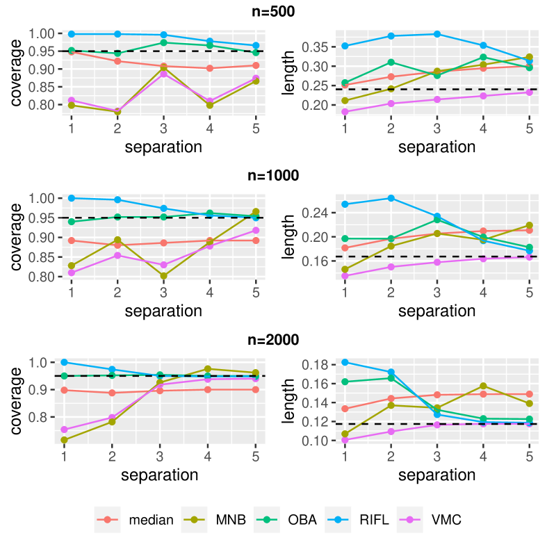
Figure 2: Low-dimensional prediction: coverage and length of $95\%$ CIs for $\beta^{*}=\theta^{*}_{1}$ with 6 majority sites and varying separation levels where $1$ is the lowest (hardest to detect) and $5$ is the highest (easiest to detect). “median” stands for the CI based on the median estimator, “MNB” stands for the m-out-of-n bootstrap CI in (38), “VMC” stands for the voting with maximum clique estimator and its associated CI in (10), “OBA” stands for the oracle bias aware CI in (39), and “RIFL” stands for our proposed CI in (19). Results are based on 500 simulation replications. Dash lines in the left panels correspond to a nominal coverage level of 0.95; in the right panels correspond to the width of an oracle CI knowing the prevailing set.

As reported in Figure 2, the RIFL CIs achieve nominal coverage across all separation levels and have an average length nearly as short as the OBA when the separation level is high. The CI of the VMC estimator shows below nominal coverage when the separation level is low or moderate. Only when the separation level is high, and the sample size is large does the VMC estimator have close to nominal coverage. This happens due to the error in separating the majority group and the remaining sites. As explained in Section 2.4, the CI based on the median estimator has coverage below the nominal level due to its bias. In this case, as the parameter values in the non-majority sites fall on both sides of $\beta^{*}$, the bias is moderate, and the coverage generally only drops to $90\%$. The CIs based on m-out-of-n bootstrap tend to undercover with low or moderate separation levels. This observation matches the discussion in Andrews (2000); Guo et al. (2021a); the MNB may not provide valid inference in non-regular settings. Recall that we chose $m=n^{\upsilon}$ with $\upsilon=0.8$. In Appendix C of the supplementary materials, we present the results of MNB based on various choices of $\upsilon$. Our results indicate that for the range of values of $\upsilon$ we explored, the MNB method tends to undercover when the separation level is low.

6.2 Multi-source high-dimensional prediction simulation

We next examine the performance of RIFL for the high-dimensional multi-source prediction problem described in subsection 5.2 with a continuous outcome and $d=500$ covariates. For $1\leq l\leq L,$ the covariates $\{X_{i}\}_{1\leq i\leq n_{l}}$ are i.i.d. generated from a multivariate normal distribution with mean $\bm{0}$ and covariance $\Sigma/2$, where $\Sigma_{j,k}=0.6^{|j-k|}$ for $1\leq j,k\leq d$. For the $l$-th source site, we generate the outcome $Y^{(l)}$ according to the following model $Y_{i}^{(l)}=\mu_{l}+[X_{i}^{(l)}]^{\top}\theta^{(l)}+\varepsilon_{i}^{(l)},$ for $1\leq i\leq n_{l},$ with $\varepsilon_{i}^{(l)}\sim N(0,1)$. We let $\mu_{l}=0.05$ for $l\in\{1,2,3,7,9\}$ and $0$ otherwise, and set $\theta^{(l)}=\theta^{*}$ for $l\in\{1,\ldots,6\}$ with $\theta^{*}_{j}=(0.1j-0.6)\mathbf{1}(1\leq j\leq 11)$ to represent sparse signal and varying signal strength. For the non-majority sites, we set $\theta_{j}^{(7)}=\theta_{j}^{(8)}=\theta_{j}^{*}+0.2+0.05a$ and $\theta_{j}^{(9)}=\theta_{j}^{(10)}=\theta_{j}^{*}+0.15+0.05a$ for $6\leq j\leq 11$. We define $\beta^{(l)}=\theta_{11}^{(l)}$ and focus on inference for $\beta^{*}=\theta_{11}^{*}$ in the following. Additional results for $\theta_{8}^{*}$ are given in Appendix C in the supplementary materials. We vary $a$ in $\{1,2,3,4,5\}$ to represent varying levels of separation between the majority and non-majority sites. Due to the high computation cost, we do not implement the m-out-of-n bootstrap method.

In Figure 3, we present the empirical coverage and average length of the CIs from different methods. The CI coverage based on the median estimator is even lower compared to the previous example in Section 6.1, suffering from more severe bias since the parameter values in the non-majority sites are biased in the same direction. More specifically, when there are 6 majority sites, the median estimator corresponds to the average of the largest and second-largest site-specific estimators from the majority sites; see more discussions in Section 2.4.

When $n=500$, the VMC CI has consistently low coverage. This is because, with a limited sample size, we do not have enough statistical power to detect even the largest separation level we considered (corresponding to $a=5$.) As a result, some non-majority sites were wrongly included in the estimated prevailing set. When the sample size increases to $n=1000$ and $2000$, the VMC CI achieves nominal coverage when the separation level is sufficiently large but still undercovers when the separation level is low. The OBA and the RIFL CIs achieve the desired coverage across all settings. However, when $n=500$, the OBA interval gets longer as the separation level grows. As we discussed earlier, some non-majority sites were included in the estimated prevailing set regardless of the separation level due to the limited sample size. In fact, the bias of the VMC estimator resulting from these wrongly selected sites increases as the separation level increases since the non-majority sites are further away from the majority sites. The OBA CI accounts for this increasing bias and becomes longer as the separation level increases. Moreover, when $n=1000$, the OBA interval is much longer than the RIFL interval for small to moderate separation levels. This is again due to the OBA interval correcting for the bias of the VMC estimator, which can be as large as the empirical standard error of the VMC estimator. Across all settings, the RIFL CI has a length comparable to that of the OBA and is often shorter.

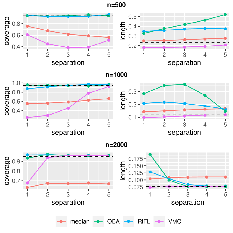
Figure 3: High-dimensional prediction: coverage and length of $95\%$ CIs for $\beta^{*}=\theta^{*}_{11}$ with 6 majority sites and varying separation levels where $1$ is the lowest (hardest to detect) and $5$ is the highest (easiest to detect). “median” stands for the CI based on the median estimator, “VMC” stands for the voting with maximum clique estimator and its associated CI in (10), “OBA” stands for the oracle bias aware CI in (39), and “RIFL” stands for our proposed CI in (19). Results are based on 500 simulation replications. Dash lines in the left panels correspond to a nominal coverage level of 0.95; in the right panels correspond to the width of an oracle CI knowing the prevailing set.

6.3 Multi-source causal simulation

We evaluate the performance of RIFL for the multi-source causal modeling problem where the interest lies in making inferences for the ATE of the target population, as described in subsection 5.3. We consider a 10-dimensional covariate vector, that is, $p=10$. For $l\in\{1,\ldots,L\}$, the covariates $\{X_{i}^{(l)}\}_{1\leq i\leq n_{l}}$ are i.i.d. generated following a multivariate normal distribution with mean $\mu_{X}^{(l)}$ and covariance matrix $\Sigma$ where $\Sigma_{jk}=0.6^{|j-k|}$ for $1\leq j,k\leq p$. For $l\in\{1,2,3,7,9\}$, we set $\mu_{X}^{(l)}$ to $\bm{0}$; and for $l\in\{4,5,6,8,10\}$, we set $\mu_{X}^{(l)}$ to $(0.5,0.5,0,0,\ldots,0)$. For $1\leq i\leq n_{l}$, given $X_{i}^{(l)}$, the treatment assignment is generated according to the conditional distribution $A_{i}^{(l)}|X_{i}^{(l)}\sim\textnormal{Bernoulli}\{\textnormal{expit}(\alpha_{1}^{(l)}X^{(l)}_{i1}+\alpha_{2}^{(l)}X^{(l)}_{i2}+\alpha_{12}^{(l)}X^{(l)}_{i1}X^{(l)}_{i2})\}$, with $\alpha_{1}^{(l)}=0.5$, $\alpha_{2}^{(l)}=-0.5$ and $\alpha_{12}^{(l)}=0.1$. The outcome for the $l$-th site is generated according to $Y_{i}^{(l)}=\mu_{l}+[X_{i}^{(l)}]^{\top}\zeta^{(l)}+\beta^{(l)}A_{i}^{(l)}+\varepsilon_{i}^{(l)},$ with $\varepsilon_{i}^{(l)}\sim N(0,1)$ for $1\leq i\leq n_{l}.$ Here, the regression coefficient $\zeta^{(l)}$ is set to $(0.5,0.5,0.5,0.5,0.5,0.1,0.1,0.1,0,0)$ across all sites and the site-specific intercept $(\mu_{1},\mu_{2},\ldots,\mu_{10})$ is set to $(0.05,-0.05,0.1,-0.1,0.05,-0.05,0.1,-0.1,0,0)$. The coefficient $\beta^{(l)}$ measures the treatment effect. For the majority sites, that is, $l\in\{1,\ldots,6\}$, $\beta^{(l)}=-1$. We set $\beta^{(7)}=\beta^{(8)}=-1-0.2a$ and $\beta^{(9)}=\beta^{(10)}=-1-0.1a$, where $a\in\{1,2,3,4,5\}$ controls the degree of separation. The covariate in the target population is generated from multivariate normal with mean $\bm{0}$ and covariance matrix $\Sigma$. We generated $N=10,000$ realizations of $X$ from the target population when evaluating the ATE.

To estimate the outcome regressions, we fit a linear model with the main effects of each covariate within the treatment arm in each site. The propensity score is estimated via a logistic model with main effects of $X_{\cdot,1}^{(l)}$ and $X_{\cdot,2}^{(l)}$ only within each site. Finally, we assume the following model for the density ratio, $\omega_{l}(X_{i}^{(l)};\bm{\eta}^{(l)})=\exp([\bm{\eta}^{(l)}]^{\top}\widetilde{X}_{i}^{(l)})$, where $\widetilde{X}_{i}^{(l)}=(1,(X_{i}^{(l)})^{\top})^{\top}$. We estimate $\bm{\eta}^{(l)}$ by solving the estimating equation $\sum_{i=1}^{n}\exp([\bm{\eta}^{(l)}]^{\top}\widetilde{X}_{i}^{(l)})\widetilde{X}_{i}^{(l)}/n=\sum_{j=1}^{N}\widetilde{X}_{j}^{\mathcal{T}}/N$, where $\widetilde{X}_{j}^{\mathcal{T}}=(1,(X_{j}^{\mathcal{T}})^{\top})^{\top}$ and $X_{j}^{\mathcal{T}}$ denotes the $j$-th observation in the target dataset, for $j\in\{1,\ldots,N\}$. It is worth noting that, although the propensity score model is misspecified, the double robustness property guarantees that the resulting estimator is still consistent and asymptotically normal given that the outcome regression model is correctly specified.

Plots of empirical coverage and average length of the CIs produced via various methods based on 500 simulation replications are provided in Figure 4 for 6 majority sites. We observe similar patterns as in the low-dimensional prediction example in Section 6.1. In particular, the coverage of VMC CI approaches the nominal level as the level of separation and sample size increase, but is generally below the nominal level when separation is small to moderate. The MNB CI also undercovers when separation is not sufficiently large. Both RIFL and OBA achieve the nominal coverage across all settings and their length are generally comparable. In this case, the coverage of the CI based on the median estimator is low because the average treatment effects in the non-majority sites are all smaller than that in the majority sites, and therefore the median estimator suffers from severe bias.

6.4 Robustness to different choices of tuning parameters

We empirically assess the sensitivity of coverage and precision of the RIFL CIs to the choices of the tuning parameter $\rho(M)$ and the resampling size $M.$ We continue with the low-dimensional multi-source prediction problem in Section 6.1 where the majority rule is satisfied with 6 majority sites and $n_{l}=n=1000$ for $1\leq l\leq 10$. Moreover, we set the separation level $a=3$. As reported in Figure 5, the RIFL CIs vary slightly with different choices of resampling size $M$ (500, 1,000, or 5,000) in terms of both empirical coverage and average length. As discussed in Section 3.3, we choose the smallest $\rho(M)$ such that more than a proportion (prop) of the resampled sets satisfy the majority rule. We test sensitivity to the choice of $\rho(M)$ by varying the proportion (prop) from $5\%$ to $50\%$ with a $5\%$ increment. In Figure 5, we observe that the RIFL CIs with different choices of $\rho(M)$ achieve the desired coverage. The average lengths of the RIFL CIs increase with the proportion.

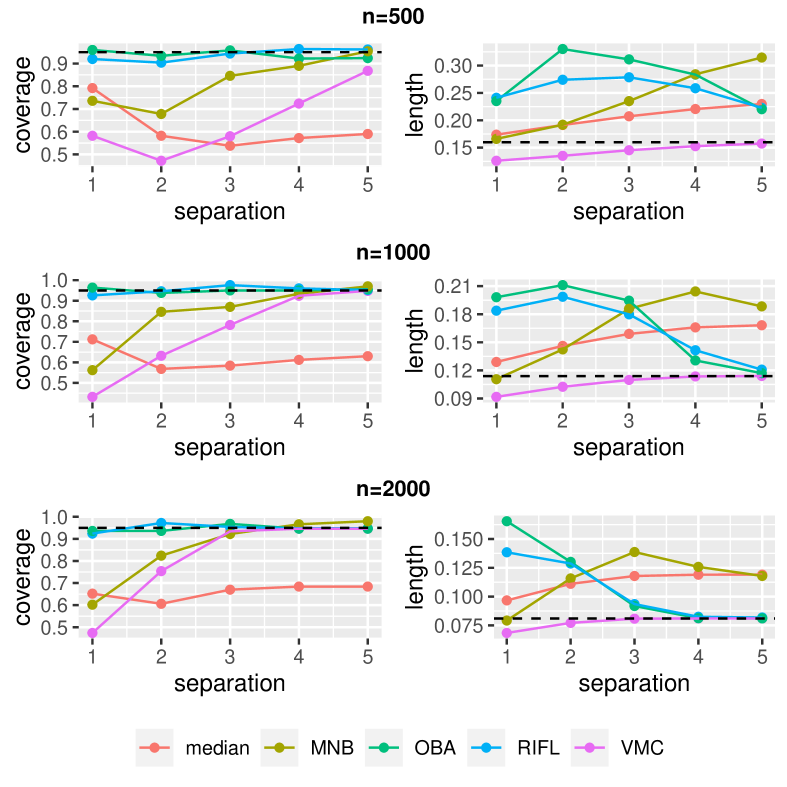
Figure 4: Causal inference: coverage and length of $95\%$ CIs for target ATE of the prevailing sites with 6 majority sites and varying separation levels where $1$ is the lowest (hardest to detect) and $5$ is the highest (easiest to detect). “median” stands for the CI based on the median estimator, “MNB” stands for the m-out-of-n bootstrap CI in (38), “VMC” stands for the voting with maximum clique estimator and its associated CI in (10), “OBA” stands for the oracle bias aware CI in (39), and “RIFL” stands for our proposed CI in (19). Results are based on 500 simulation replications. Dash lines in the left panels correspond to a nominal coverage level of 0.95; in the right panels correspond to the width of an oracle CI knowing the prevailing set.

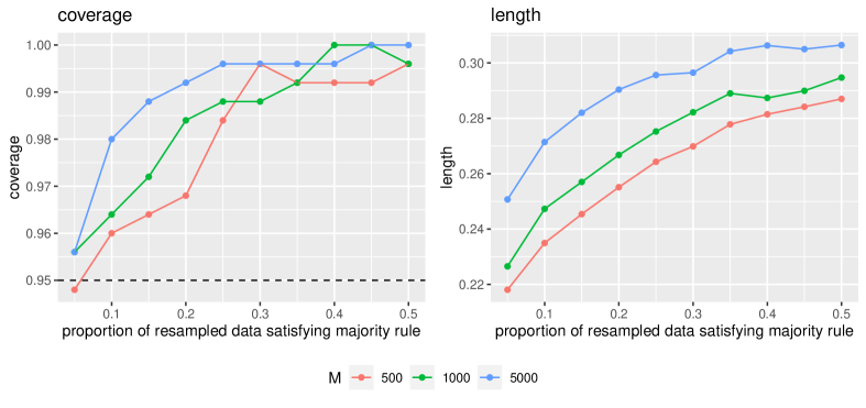
Figure 5: Sensitivity of coverage and the average length of the RIFL CI to different $M$ and $\rho(M)$. Results are based on 200 simulation replications. The x-axis represents the value prop, where the tuning parameter $\rho(M)$ is chosen as the smallest value such that more than prop of the resampled dissimilarity measures produce maximum clique sets satisfying the majority rule.

7 RIFL Integrative Analysis of EHR Studies on COVID-19 Mortality Prediction

Severe acute respiratory syndrome coronavirus 2 (SARS-CoV-2) has led to millions of COVID-19 infections and death. Although most individuals present with only a mild form of viral pneumonia, a fraction of individuals develop severe disease. COVID-19 remains a deadly disease for some, including elderly and those with compromised immune systems (Wu and McGoogan, 2020; Goyal et al., 2020; Wynants et al., 2020). Identifying patients at high risk for mortality can save lives and improve the allocation of resources in resource-scarce health systems.

To obtain a better understanding of mortality risk for patients hospitalized with COVID-19, we implement our RIFL algorithm using data assembled by $L=16$ healthcare centers from four countries, representing $275$ hospitals as part of the multi-institutional Consortium for the Clinical Characterization of COVID-19 by EHR (4CE) (Brat et al., 2020). To be included in the study, patients were required to have a positive SARS-CoV-2 reverse transcription polymerase chain reaction (PCR) test, a hospital admission with a positive PCR test between March 1, 2020 and January 31, 2021, and the hospital admission to have occurred no more than seven days before and no later than 14 days after the date of their first positive PCR test. Patients who died on the day of admission were excluded. In the RIFL analysis, we focused on the subset of sites whose summary level data including the covariance matrices of the mortality regression models were available, resulting in a total of 42,655 patients for analyses. Due to patient privacy constraints, individual-level data remained within the firewalls of the institutions, while summary-level data have been generated for a variety of research projects (e.g., Weber et al., 2022).

We focus on baseline risk factors that were measured in all 16 sites. These baseline risk factors included age group (18-25, 26-49, 50-69, 70-79, 80+), sex, pre-admission Charlson comorbidity score, and nine laboratory test values at admission: albumin, aspartate aminotransferase (AST), AST to alanine aminotransferase ratio (AST/ALT), bilirubin, creatinine, C-reactive protein (CRP), lymphocyte count, neutrophil count, and white blood cell (WBC) count. Laboratory test data had relatively low missingness $(<30\%)$, and missing values were imputed via multivariate imputation by chained equations and averaged over five imputed sets.

We aim to identify and estimate a prevailing mortality risk prediction model to better understand the effect of baseline risk factors on mortality. Specifically, for each healthcare center $l$, $1\leq l\leq 16$, we let $\theta^{(l)}\in\mathbb{R}^{15}$ denote the vector of log hazard ratios associated with the 15 risk factors, that is, the vector of regression coefficients in a multivariate Cox model. We make statistical inferences for the log hazard ratio associated with each risk factor and let $\beta^{(l)}=\theta^{(l)}_{j}$ while varying $j$ from 1 to 15. We fit Cox models with adaptive LASSO penalties to obtain $\widehat{\theta}^{(l)}$, the estimated log hazard ratios of the $15$ baseline risk factors on all-cause mortality within 30-days of hospitalization. Since the sample size is relatively large compared to $p=15$, we expect the oracle property of the adaptive LASSO estimator to hold and hence can rely on asymptotic normality for these local estimators along with consistent estimators of their variances (Zou, 2006).

We implement in Figure 6 both RIFL and VMC to generate $95\%$ CIs for each baseline risk factor. For RIFL, we set $M=500$ and choose the value of $\rho(M)$ according to Section 3.3. That is, we start with a small value (e.g., $1/12$) and set $\rho(M)$ to be the smallest value below 1 such that more than $10\%$ of the resampled dissimilarity measures produce maximum clique sets satisfying the majority rule. The generalizability measures $\{\widehat{p}_{l}\}_{1\leq l\leq 16}$, defined as $\widehat{p}_{l}={\sum_{m\in\mathcal{M}}{\bf 1}(l\in\widetilde{\mathcal{V}}^{[m]})}/{|\mathcal{M}|}$, represent the proportion of times that healthcare center $l$ was included in the majority group. Note that we can calculate a set of generalizability measures for the 16 sites for each risk factor. A visualization of the full generalizability measure is given in Figure C7 in the supplement.

As reported in Figure 6, the RIFL and VMC intervals are mostly comparable, although for some risk factors, the RIFL CI is notably longer than the VMC CI. However, as we demonstrated in the simulation studies, VMC CI may suffer from under-coverage due to site selection errors. Indeed, some sites have low generalizability scores when we focus on a particular risk factor. For example, site 4 has a generalizability measure of 0.020 when we focus on the variable of age group 18-25; and site 2 has a generalizability measure of 0.016 when we focus on the variable of age $>80$. This suggests that these sites are not aligned well with other sites when we study the effect of the corresponding risk factor. However, VMC included these sites in the estimated prevailing sets, and the resulting CIs can be misleading. In general, across all 15 risk factors, most sites except for sites 2 and 4 have high generalizability measures, as shown in Figure C7 of the supplement.

Our results indicate that older age, male sex, higher Charlson comorbidity score, lower serum albumin level, and higher creatinine, CRP and AST levels are associated with higher mortality risk for patients hospitalized with a positive PCR COVID-19 test. The laboratory tests predictive of mortality represent a mix of general health status (e.g., serum albumin), renal function (e.g., creatinine), hepatic function (e.g., AST), and acute inflammatory response (e.g., CRP). These results are consistent with previous findings in related studies of laboratory measurements to predict COVID-19 mortality (Weber et al., 2022). Recent literature suggests that measuring serum albumin can identify COVID-19 infected patients who are more likely to progress to severe disease and that serum albumin can serve as a useful marker for disease progression (Turcato et al., 2022). Our results corroborate this finding. The use of regularly collected laboratory tests, in addition to baseline demographic and comorbidity information, can aid in the development of a clinically useful prediction tool for mortality risk following hospital admission with COVID-19. Patients identified as having a high risk for mortality could then be prioritized for closer monitoring and potentially more aggressive interventions when deemed appropriate by the physician.

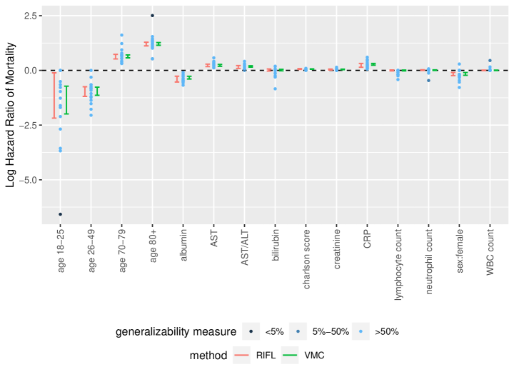
Figure 6: RIFL and VMC $95\%$ CIs for log hazard ratios of mortality within 14 days of hospitalization with COVID-19 for each of the $15$ baseline risk factors. Dots represent the point estimates from individual sites, and darker color of the dots corresponds to lower generalizability measure of individual sites.

8 Conclusion and Discussion

The RIFL confidence interval, robust to the errors in separating the non-majority sites from the majority sites, guarantees uniformly valid coverage of the prevailing model. When the majority of sites are well separated from the other sites, the RIFL CI performs similarly to the oracle CI assuming the knowledge of the majority group.

The majority rule is a crucial assumption for our proposal, and an empirical assessment of the majority rule is vital to validate our proposed procedure. Our proposed RIFL method might provide a heuristic assessment of the majority rule. Suppose the index set $\mathcal{M}$ defined in (16) has the cardinality below $10\%\cdot M$ even for $\rho$ approaching $1$. In that case, we claim that the majority rule may fail since it is difficult to verify the majority rule with most of the resampled data. As a relaxation of the majority rule, we might relax the strict equality of the definition of $\mathcal{V}(\theta)$ in (1) to approximate equality,

$$\mathcal{V}_{\kappa}(\theta)\coloneqq\{1\leq l\leq L:\|\theta^{(l)}-\theta\|_{2}\leq\kappa\},\quad\text{for some}\quad\kappa>0.$$ (40)

When $\kappa$ is sufficiently close to zero, our main results may be generalized to hold under the majority rule (Assumption 1) defined with $\mathcal{V}_{\kappa}(\theta)$.

In practice, domain experts might believe that more than $50\%$ (e.g. $80\%$) of the total sites are similar. Our proposed RIFL can be directly extended to accommodate additional prior information. For example, we may consider the 80% rule; that is, the domain experts expect more than 80% of the sites to share the parameters of interest. We can modify our construction by replacing $L/2$ in (16) and (17) with $80\%\cdot L.$ Importantly, the RIFL methods leveraging either the majority rule or the 80% rule will guarantee uniformly valid CIs for the parameter of the prevailing model, provided that there are indeed more than $80\%$ of the sites in the prevailing set. However, the RIFL leveraging the 80% rule will have a shorter length due to the additional prior information, as shown in Section C.1 of the supplement where we compare the coverage and lengths of RIFL CIs under different prior knowledge. It is also possible to consider alternative strategies for choosing $\rho$ to incorporate further data-adaptive assessment of prevailing set size based on $\{\widehat{p}_{l}\}_{1\leq l\leq L}$. Theoretically justified approaches to adaptively choose $\rho(M)$ warrant further research.

We discuss two possible directions for robust information aggregation when the majority rule or its relaxed version does not hold. Firstly, the target prediction model can be defined as the one shared by the largest number of sites. If we cluster $\{\theta^{(l)}\}_{1\leq l\leq L}$ into subgroups according to their similarity, the group of the largest size naturally defines a target model, even though this largest group does not contain more than $L/2$ sites. Secondly, we can define the set $\mathcal{V}_{\kappa}(\theta)$ in (40) with a relatively large $\kappa$, that is, $\mathcal{V}_{\kappa}(\theta)$ contains all sites with the parameters similar to but possibly different from $\theta$. We may still pool over the information belonging to $\mathcal{V}_{\kappa}(\theta)$ through defining a group distributionally robust model as in Meinshausen and Bühlmann (2015); Hu et al. (2018); Sagawa et al. (2019); Guo (2020). The post-selection problem persists in both settings. It is arguably vital to account for the uncertainty in identifying useful sites. Our proposal is potentially useful to account for the site selection and make inferences for these target models, which is left to future research.

Appendix A Extra Method and Theory

A.1 RIFL Algorithm

Algorithm 1 Proposed sampling method for the multi-source inference

Input: Site-specific estimators $\{\widehat{\beta}^{(l)},\widehat{\sigma}_{l}\}_{1\leq l\leq L};$ dissimilarity measures $\{\widehat{\mathcal{D}}_{l,k}\}_{1\leq l<k\leq L}$ with SE estimates $\{\widehat{\rm SE}(\widehat{\mathcal{D}}_{l,k})\}_{1\leq l<k\leq L}$; $M\geq 1$, $\rho(M)\in(0,1)$, and levels $\nu,\alpha>0$.

Output: Confidence interval ${\rm CI}$; measure of generalizability for each site

1:for $l\leftarrow 1$ to $L-1$ do

2:     for $k\leftarrow l+1$ to $L$ do

3:         Compute $\widehat{{\mathcal{L}}}_{l,k}=\widehat{\beta}^{(l)}-\widehat{\beta}^{(k)}$ and $\widehat{\rm SE}(\widehat{{\mathcal{L}}}_{l,k})=\sqrt{\widehat{\sigma}_{l}^{2}+\widehat{\sigma}_{k}^{2}}$;

4:     end for

5:end for

6:for $m\leftarrow 1$ to $M$ do

7:     Resample the dissimilarity measures $\{\widehat{\mathcal{D}}^{[m]}_{l,k},\widehat{{\mathcal{L}}}^{[m]}_{l,k}\}_{1\leq l<k\leq L}$ as in (11);

8:     Compute the resampled test statistics $\{\widehat{S}^{[m]}_{l,k}\}_{1\leq l<k\leq L}$ as in (12);

9:     Construct the sampled voting matrix $\widehat{H}^{[m]}$ as in (14);

10:     Construct the maximum clique $\widehat{\mathcal{V}}^{[m]}$ as in (15);

11:     Construct the aggregation set $\widetilde{\mathcal{V}}^{[m]}$ as in (17);

12:     Construct the confidence interval ${\rm CI}^{[m]}$ as in (18);

13:end for

14:Construct the index set $\mathcal{M}$ as in (16);

15:Return the ${\rm CI}$ defined in (19);

16:for $l\leftarrow 1$ to $L$ do

17:     Return the generalizability measure $\widehat{p}_{l}={\sum_{m\in\mathcal{M}}{\bf 1}(l\in\widetilde{\mathcal{V}}^{[m]})}/{|\mathcal{M}|}$;

18:end for

A.2 Theoretical properties of $\widehat{\mathcal{D}}_{l,k}$ in high dimensions

We summarize our proposed estimators of high-dimensional distance measures in the following Algorithm 2.

Algorithm 2 High-dimensional Distance Measures

Input: the multi-source data $\{X^{(l)},Y^{(l)}\}_{1\leq l\leq L}$.

Output: $\{\widehat{\beta}^{(l)},\widehat{\rm SE}(\widehat{\beta}^{(l)}),\widehat{\mathcal{D}}_{l,k},\widehat{\rm SE}(\widehat{\mathcal{D}}_{l,k})\}_{1\leq l<k\leq L}$

1:for $l\leftarrow 1$ to $L$ do

2:     Compute the initial $\widetilde{\mu}_{l},\widetilde{\theta}^{(l)}$ as in (29);

3:     Compute $\widehat{\beta}^{(l)}$ and ${\rm SE}(\widehat{\beta}^{(l)})$ satisfying (30);

4:end for

5:Broadcast $\{\widetilde{\mu}_{l},\widetilde{\theta}^{(l)},\widehat{\beta}^{(l)},\widehat{\rm SE}(\widehat{\beta}^{(l)})\}_{1\leq l\leq L}$ to all $L$ sites;

6:for $l\leftarrow 1$ to $L$ do

7:     Compute the projection direction $\{\widehat{u}_{k}^{(l)}\}_{k\neq l}$ as in (33);

8:     Compute $\{\widehat{\delta}^{(l)}_{k}\}_{k\neq l}$ as in (34) and $\{\widehat{\rm V}^{(l)}_{k}\}_{k\neq l}$ as in (35);

9:end for

10:Compute $\{\widehat{\mathcal{D}}_{l,k}\}_{1\leq k<l\leq L}$ as in (36) and $\{\widehat{\rm SE}(\widehat{\mathcal{D}}_{l,k})\}_{1\leq k<l\leq L}$ as in (37).

We shall consider the high-dimensional linear or logistic model and establish the theoretical properties of $\widehat{\mathcal{D}}_{l,k}.$ We recall the notations from the main paper. For $1\leq l\leq L$, we define $\bm{\eta}^{(l)}=(\mu_{l},[\theta^{(l)}]^{\intercal})^{\intercal}\in\mathbb{R}^{d+1}$ and $\widetilde{\bm{\eta}}^{(l)}=(\widetilde{\mu}_{l},[\widetilde{\theta}^{(l)}]^{\intercal})^{\intercal}\in\mathbb{R}^{d+1}$ and $\widetilde{X}^{(l)}_{i}=(1,(X^{(l)}_{i})^{\intercal})^{\intercal}$ for $1\leq i\leq n_{l}.$ Let $\widetilde{\gamma}_{l,k}\coloneqq(0,[\widetilde{\theta}^{(l)}-\widetilde{\theta}^{(k)}]^{\intercal})^{\intercal}$ and $\gamma_{l,k}\coloneqq(0,[\theta^{(l)}-\theta^{(k)}]^{\intercal})^{\intercal}$ for $1\leq l<k\leq L$. When it is clear from the context, we shall write $\widetilde{\gamma}$ and $\gamma$ for $\widetilde{\gamma}_{l,k}$ and $\gamma_{l,k},$ respectively.

Our theoretical analysis follows from that in Guo et al. [2021a]. We generate the model assumptions in Guo et al. [2021a] to the settings with $L$ high-dimensional regression models.

1. For $1\leq l\leq L,$ the rows $\{\widetilde{X}^{(l)}_{i}\}_{1\leq i\leq n}$ are i.i.d. $d$-dimensional Sub-gaussian random vectors with $\Sigma^{(l)}={\mathbf{E}}(\widetilde{X}^{(l)}_{i}[\widetilde{X}^{(l)}_{i}]^{\intercal})$ where $\Sigma^{(l)}$ satisfies $c_{0}\leq\lambda_{\min}\left(\Sigma^{(l)}\right)\leq\lambda_{\max}\left(\Sigma^{(l)}\right)\leq C_{0}$ for some positive constants $C_{0}\geq c_{0}>0$; The high-dimensional vector $\eta^{(l)}$ is assumed to be of less than $s$ non-zero entries.

Condition (A1) imposes the tail condition for the high-dimensional covariates and assumes that the population second-order moment matrix is invertible.

For the high-dimensional logistic regression, we impose the following condition,

1. With probability larger than $1-d^{-c}$, $\min\{h([\widetilde{X}^{(l)}_{i}]^{\intercal}{\eta}^{(l)}),1-h([\widetilde{X}^{(l)}_{i}]^{\intercal}{\eta}^{(l)})\}\geq c_{\min}$ for $1\leq i\leq n$ and some small positive constant $c_{\min}\in(0,1)$.

Condition ${\rm(A2)}$ is imposed such that the case probability is uniformly bounded away from $0$ and $1$. Condition (A2) holds for the setting with bounded $[\widetilde{X}^{(l)}_{i}]^{\intercal}\eta^{(l)}$ for $1\leq i\leq n$ with a high probability.

We assume that the penalized MLE estimator $\widetilde{\theta}^{(l)}$ satisfies the following property:

1. With probability greater than $1-d^{-c}-\exp(-cn)$ for some constant $c>0$,

   $$\|\widetilde{\eta}^{(l)}-\eta^{(l)}\|_{1}\leq Cs\left({\log d}/{n}\right)^{1/2}\quad\text{and}\quad\|\widetilde{\eta}^{(l)}_{S_{l}^{c}}-{\eta}^{(l)}_{S_{l}^{c}}\|_{1}\leq C_{0}\|\widetilde{\eta}^{(l)}_{S_{l}}-{\eta}^{(l)}_{S_{l}}\|_{1}$$

   where $S_{l}$ denotes the support of $\eta^{(l)}$ and $C>0$ and $C_{0}>0$ are positive constants.

In the high-dimensional linear model, Theorem 7.2 of Bickel et al. [2009] established that the Lasso estimator satisfies the condition (B). In the high-dimensional logistic regression, see Proposition 1 of Guo et al. [2021a] for an example of establishing that the penalized MLE estimator $\widetilde{\theta}^{(l)}$ defined in (29) satisfies the condition ${\rm(B)}$; see also the references within there.

Theorem 5

Suppose that Conditions (A1) and (B) hold for the high-dimensional linear regression or Conditions (A1), (A2), and (B) hold for the high-dimensional logistic regression, $\tau_{n}\asymp(\log n)^{1/2}$ defined in (33) satisfies $\tau_{n}{s\log d}/{\sqrt{n}}\rightarrow 0$. For any constant $0<\alpha<1$, the dissimilarity estimator $\widehat{\mathcal{D}}_{l,k}$ defined in (36) and the standard error estimator ${\widehat{\rm SE}(\widehat{\mathcal{D}}_{l,k})}$ defined in (37) satisfy (3) for $1\leq l<k\leq L.$

We present the proof of the above theorem in Section B.5.

A.3 Influence function of the doubly robust ATE estimator

For an i.i.d. sample from the $l$-th source population of size $n_{l}$, we use $X_{i}^{(l)}\in\mathbb{R}^{p}$ to denote the covariate vector in the $i$-th observation and $X_{ij}^{(l)}\in\mathbb{R}$ to denote the $j$-th covariate in the $i$-th observation.

We consider the case where the outcome regression functions and the propensity score are estimated with generalized linear models (GLMs). Specifically, for the propensity score model, we fit the following GLM:

$$\mathbf{E}\left[A^{(l)}|X^{(l)}\right]=h\left(\alpha_{l,0}+\sum_{j=1}^{B}\alpha_{l,j}\psi_{j}(X^{(l)})\right)=h\left(\bm{\alpha}_{l}^{\top}\widetilde{X}^{(l)}\right),$$

where $\{\psi_{1}(\cdot),\ldots,\psi_{B}(\cdot)\}$ is a set of basis functions, $\widetilde{X}^{(l)}=(1,\psi_{1}(X^{(l)}),\ldots,\psi_{B}(X^{(l)}))^{\top}$ and $\bm{\alpha}_{l}=(\alpha_{l,0},\alpha_{l,1},\ldots,\alpha_{l,B})$. One simple example is to take $\psi_{j}(X_{i}^{(l)})=X_{ij}^{(l)}$ for $j\in\{1,\ldots,p\}$, and we get a GLM that includes the main effect of each covariate. We estimate the coefficient by solving the following estimating equation:

$$\frac{1}{n_{l}}\sum_{i=1}^{n_{l}}\widetilde{X}_{i}^{(l)}\left\{A_{i}^{(l)}-h\left(\bm{\alpha}^{\top}\widetilde{X}_{i}^{(l)}\right)\right\}=0,$$

and obtain an estimated coefficient which we denote as $\widehat{\bm{\alpha}}_{l}$.

For the outcome regressions, we fit generalized linear models within each treatment arm in each source site:

$$\mathbf{E}(Y^{(l)}\mid A^{(l)}=a,X^{(l)})=g\left(\bm{\gamma}_{a,0}^{(l)}+\sum_{j=1}^{B_{\bm{\gamma}}}\bm{\gamma}^{(l)}_{a,j}\phi_{j}(X^{(l)})\right)=g\left([W^{(l)}]^{\top}\bm{\gamma}^{(l)}_{a}\right),\quad\textnormal{ for }a\in\{0,1\},$$

where $W^{(l)}=(1,\phi_{1}(X^{(l)}),\ldots,\phi_{B_{\bm{\gamma}}}(X^{(l)}))$ for some set of basis functions $\{\phi_{1}(\cdot),\ldots,\phi_{B_{\bm{\gamma}}}(\cdot)\}$, and $\bm{\gamma}^{(l)}_{a}=(\bm{\gamma}_{a,0}^{(l)},\bm{\gamma}^{(l)}_{a,1},\ldots,\bm{\gamma}^{(l)}_{a,B_{\bm{\gamma}}})$. Let $I\{\cdot\}$ denote the indicator function. We estimate the coefficients $\bm{\gamma}^{(l)}_{a}$ by solving the following estimating equation:

$$\frac{1}{n_{l}}\sum_{i=1}^{n_{l}}I\left\{A^{(l)}_{i}=a\right\}W^{(l)}_{i}\left\{Y^{(l)}_{i}-g\left([W^{(l)}_{i}]^{\top}\bm{\gamma}^{(l)}_{a}\right)\right\}=0,$$

and we denote the estimate as $\widehat{\bm{\gamma}}^{(l)}_{a}$.

For the density ratio, we consider an exponential tilt model, $\omega_{l}(X^{(l)};\bm{\eta}^{(l)})=\exp([\bm{\eta}^{(l)}]^{\top}\widetilde{W}^{(l)})$, where $\widetilde{W}^{(l)}=(1,\varphi_{1}(X^{(l)}),\ldots,\varphi_{B_{\omega}}(X^{(l)}))^{\top}$for a set of basis functions $\{\varphi_{1}(\cdot),\ldots,\varphi_{B_{\omega}}(\cdot)\}$. We estimate the parameter $\bm{\eta}^{(l)}$ by solving the following estimating equation

$$\frac{1}{n_{l}}\sum_{i=1}^{n_{l}}\exp\left([\bm{\eta}^{(l)}]^{\top}\widetilde{W}_{i}^{(l)}\right)\widetilde{W}_{i}^{(l)}=\frac{1}{N}\sum_{j=1}^{N}\widetilde{W}_{j}^{\mathcal{T}}/N$$

where $\widetilde{W}_{j}^{\mathcal{T}}=(1,\varphi_{1}(X_{j}^{\mathcal{T}}),\ldots,\varphi_{B_{\omega}}(X_{j}^{\mathcal{T}}))^{\top}$ and $X_{j}^{\mathcal{T}}$ denotes the $j$-th observation in the target dataset, for $j\in\{1,\ldots,N\}$. We denote the resulting estimate by $\widehat{\bm{\eta}}^{(l)}$. Essentially, we estimate the parameter $\bm{\eta}^{(l)}$ by matching the sample mean of a set of basis functions in the source dataset and the much larger target dataset.

Let $\bm{\alpha}_{l}^{*}$, $\bm{\gamma}_{0}^{(l),*}$,$\bm{\gamma}_{1}^{(l),*}$ and $\bm{\eta}^{(l),*}$ denote the probabilistic limits of $\widehat{\bm{\alpha}}_{l}$, $\widehat{\bm{\gamma}}^{(l)}_{0}$, $\widehat{\bm{\gamma}}^{(l)}_{1}$ and $\widehat{\bm{\eta}}^{(l)}$, respectively. The precise definitions of these population parameters are given in the proof of Theorem 6. Define the following matrices:

$$C_{\bm{\alpha},l} =\mathbf{E}_{l}\left[\widetilde{X}^{(l)}h^{\prime}\left((\bm{\alpha}_{l}^{*})^{\top}\widetilde{X}^{(l)}\right)\left(\widetilde{X}^{(l)}\right)^{\top}\right];$$

$$C_{\bm{\gamma}_{a},l} =\mathbf{E}_{l}\left[I\left\{A^{(l)}=a\right\}W^{(l)}g^{\prime}\left([W^{(l)}]^{\top}\bm{\gamma}^{(l),*}_{a}\right)[W^{(l)}]^{\top}\right],\quad a\in\{0,1\};$$

$$C_{\bm{\eta},l} =-\mathbf{E}_{l}\left[\exp\left([\bm{\eta}^{(l),*}]^{\top}\widetilde{W}^{(l)}\right)\widetilde{W}^{(l)}[\widetilde{W}^{(l)}]^{\top}\right],$$

where $\mathbf{E}_{l}$ denotes the expectation with respect to the joint distribution of $(X^{(l)},A^{(l)},Y^{(l)})$ in the $l$-th source population.

Recall from Section 5.3 that the target ATE estimator takes the form $\widehat{\theta}^{(l)}=\widehat{M}^{(l)}+\widehat{\delta}^{(l)}$ where

$$\widehat{M}^{(l)}=\frac{1}{N}\sum_{i=1}^{N}\left\{m(1,X_{i}^{\mathcal{T}};\widehat{\bm{\gamma}}^{(l)}_{1})-m(0,X_{i}^{\mathcal{T}};\widehat{\bm{\gamma}}^{(l)}_{0})\right\}$$

and

$$\widehat{\delta}^{(l)} =\frac{1}{n_{l}}\sum_{i=1}^{n_{l}}\omega_{l}(X_{i}^{(l)};\widehat{\bm{\eta}}^{(l)})\left\{\sum_{a=0}^{1}\frac{(-1)^{a+1}I\{A_{i}^{(l)}=a\}}{\pi_{l}(a,X^{(l)}_{i};\widehat{\bm{\alpha}}_{l})}\{Y^{(l)}_{i}-m(A_{i}^{(l)},X^{(l)}_{i};\widehat{\bm{\gamma}}^{(l)}_{a})\}\right\}.$$

In this case, we have that

$$m(a,X_{i}^{(l)};\widehat{\bm{\gamma}}_{a}^{(l)}) =g\left([W^{(l)}_{i}]^{\top}\widehat{\bm{\gamma}}^{(l)}_{a}\right);$$

$$m(a,X_{i}^{\mathcal{T}};\widehat{\bm{\gamma}}_{a}^{(l)}) =g\left([W^{\mathcal{T}}_{i}]^{\top}\widehat{\bm{\gamma}}^{(l)}_{a}\right);$$

$$\omega_{l}(X_{i}^{(l)};\widehat{\bm{\eta}}^{(l)}) =\exp\left([\widehat{\bm{\eta}}^{(l)}]^{\top}\widetilde{W}_{i}^{(l)}\right);$$

$$\pi_{l}(a,X^{(l)}_{i};\widehat{\bm{\alpha}}_{l}) =h\left((\widehat{\bm{\alpha}}_{l})^{\top}\widetilde{X}_{i}^{(l)}\right)^{a}\left\{1-h\left((\widehat{\bm{\alpha}}_{l})^{\top}\widetilde{X}_{i}^{(l)}\right)\right\}^{(1-a)}.$$

For the ease of notation, we define the functions $\tau_{\bm{\gamma}_{0},\bm{\gamma}_{1}}(\cdot)$ and $\xi_{\bm{\eta},\bm{\alpha},\bm{\gamma}_{0},\bm{\gamma}_{1}}(\cdot)$ such that

$$\tau_{\bm{\gamma}_{0},\bm{\gamma}_{1}}(x^{(l)})=m(1,x^{(l)};\bm{\gamma}_{1})-m(0,x^{(l)};\bm{\gamma}_{0}),$$

and

$$\xi_{\bm{\eta},\bm{\alpha},\bm{\gamma}_{0},\bm{\gamma}_{1}}(x^{(l)},a^{(l)},y^{(l)})=\omega_{l}(x^{(l)};\bm{\eta})\left\{\sum_{a=0}^{1}\frac{(-1)^{a+1}I\{a^{(l)}=a\}}{\pi_{l}(a,x^{(l)};\bm{\alpha})}\{y^{(l)}-m(a,x^{(l)};\bm{\gamma}_{a}\}\right\}.$$

These functions will appear frequently in the following derivation and in the influence function of $\widehat{\theta}^{(l)}$. Also note that the functions $\tau$ and $\xi$ are indexed by the nuisance model parameters.

Define the following quantities:

$$\bm{d}_{\bm{\gamma}_{0}} =-\mathbf{E}_{\mathcal{T}}\left[g^{\prime}\left([W^{\mathcal{T}}]^{\top}\bm{\gamma}_{0}^{(l),*}\right)W^{\mathcal{T}}\right]+\mathbf{E}_{l}\left[\exp\left([\bm{\eta}^{(l),*}]^{\top}\widetilde{W}^{(l)}\right)\frac{I\{A^{(l)}=0\}}{1-h\left([\widetilde{X}^{(l)}]^{\top}\bm{\alpha}_{l}^{*}\right)}\left\{g^{\prime}\left([W^{(l)}]^{\top}\bm{\gamma}_{0}^{(l),*}\right)W^{(l)}\right\}\right];$$

$$\bm{d}_{\bm{\gamma}_{1}} =\mathbf{E}_{\mathcal{T}}\left[g^{\prime}\left([W^{\mathcal{T}}]^{\top}\bm{\gamma}_{1}^{(l),*}\right)W^{\mathcal{T}}\right]-\mathbf{E}_{l}\left[\exp\left([\bm{\eta}^{(l),*}]^{\top}\widetilde{W}^{(l)}\right)\frac{I\{A^{(l)}=1\}}{h\left([\widetilde{X}^{(l)}]^{\top}\bm{\alpha}_{l}^{*}\right)}\left\{g^{\prime}\left([W^{(l)}]^{\top}\bm{\gamma}_{1}^{(l),*}\right)W^{(l)}\right\}\right];$$

$$\bm{d}_{\bm{\eta}} =\mathbf{E}_{l}\left[\exp\left([\bm{\eta}^{(l),*}]^{\top}\widetilde{W}^{(l)}\right)\widetilde{W}^{(l)}\left\{\sum_{a=0}^{1}\frac{(-1)^{a+1}I\{A^{(l)}=a\}}{\pi_{l}(a,X^{(l)};\bm{\alpha}^{*}_{l})}\left\{Y^{(l)}-g\left([W^{(l)}]^{\top}\bm{\gamma}_{a}^{(l),*}\right)\right\}\right\}\right];$$

$$\bm{d}_{\bm{\alpha}} =\mathbf{E}_{l}\left[\exp\left([\bm{\eta}^{(l),*}]^{\top}\widetilde{W}^{(l)}\right)\left\{\sum_{a=0}^{1}\frac{-I\{A^{(l)}=a\}\pi_{l}^{\prime}(a,X^{(l)};\bm{\alpha}_{l}^{*})}{\pi_{l}^{2}(a,X^{(l)};\bm{\alpha}_{l}^{*})}\left\{Y^{(l)}-g\left([W^{(l)}]^{\top}\bm{\gamma}_{a}^{(l),*}\right)\right\}\right\}\widetilde{X}^{(l)}\right].$$

Theorem 6

When $N\gg n_{l}$, the target ATE estimator $\widehat{\theta}^{(l)}$ is asymptotically linear with influence function $\tau_{\theta}$ such that

$$\tau_{\theta}(x^{(l)},a^{(l)},y^{(l)}) =\xi_{\bm{\eta}^{(l),*},\bm{\alpha}_{l}^{*},\bm{\gamma}_{0}^{(l),*},\bm{\gamma}_{1}^{(l),*}}(x^{(l)},a^{(l)},y^{(l)})$$

$$\quad+\bm{d}_{\bm{\gamma}_{0}}^{\top}C_{\bm{\gamma}_{0},l}^{-1}I\left\{a^{(l)}=0\right\}w^{(l)}\left\{y^{(l)}-g\left([w^{(l)}]^{\top}\bm{\gamma}^{(l),*}_{0}\right)\right\}$$

$$\quad+\bm{d}_{\bm{\gamma}_{1}}^{\top}C_{\bm{\gamma}_{1},l}^{-1}I\left\{a^{(l)}=1\right\}w^{(l)}\left\{y^{(l)}-g\left([w^{(l)}]^{\top}\bm{\gamma}^{(l),*}_{1}\right)\right\}$$

$$\quad+\bm{d}_{\bm{\eta}}^{\top}C_{\bm{\eta},l}^{-1}\left\{\exp\left([\bm{\eta}^{(l),*}]^{\top}\widetilde{w}^{(l)}\right)\widetilde{w}^{(l)}-\mathbf{E}_{\mathcal{T}}\left[\widetilde{W}^{\mathcal{T}}\right]\right\}$$

$$\quad+\bm{d}_{\bm{\alpha}}^{\top}C_{\bm{\alpha},l}^{-1}\widetilde{x}^{(l)}\left\{a^{(l)}-h\left((\bm{\alpha}_{l}^{*})^{\top}\widetilde{x}^{(l)}\right)\right\}.$$

Here the vectors $\widetilde{x}^{(l)}$, $w^{(l)}$ and $\widetilde{w}^{(l)}$ denote the vectors of basis functions derived from the covariate vector $x^{(l)}$.

We present the proof of the above theorem in Section B.6.

The variance of $\widehat{\theta}^{(l)}$ can be consistently estimated by the empirical variance of the function $\widehat{\tau}_{\theta}$ on the source data, where $\widehat{\tau}_{\theta}$ is an estimate of $\tau_{\theta}$ obtained by plugging in the estimates for the nuisance model parameters $(\bm{\eta}^{(l),*},\bm{\alpha}_{l}^{*},\bm{\gamma}_{0}^{(l),*},\bm{\gamma}_{1}^{(l),*})$, the partial derivatives $(\bm{d}_{\bm{\gamma}_{0}},\bm{d}_{\bm{\gamma}_{1}},\bm{d}_{\bm{\eta}},\bm{d}_{\bm{\alpha}})$, and the matrices $C_{\bm{\gamma}_{0},l}$, $C_{\bm{\gamma}_{1},l},C_{\bm{\eta},l}$ and $C_{\bm{\alpha},l}$. Consistent estimators for these partial derivatives and matrices are given in the proof of Theorem 6.

Appendix B Proofs

B.1 Proof of Theorem 1

Denote the observed data by $\mathcal{O}$. We define the following event for the data $\mathcal{O}$,

$$\mathcal{E}=\left\{\max_{1\leq l<k\leq L}\max\left\{\frac{\left|\widehat{\mathcal{D}}_{l,k}-{\mathcal{D}}_{l,k}\right|}{\widehat{\rm SE}(\widehat{\mathcal{D}}_{l,k})},\frac{\left|\widehat{{\mathcal{L}}}_{l,k}-{{\mathcal{L}}}_{l,k}\right|}{\widehat{\rm SE}(\widehat{{\mathcal{L}}}_{l,k})}\right\}\leq z_{\nu/[2L(L-1)]}\right\}.$$ (41)

Since the site-specific estimators $\left\{\widehat{\beta}^{(l)},\widehat{\sigma}_{l}\right\}_{1\leq l\leq L}$ satisfy (2), we establish

$$\limsup_{n\rightarrow\infty}{\mathbf{P}}\left({\left|\widehat{{\mathcal{L}}}_{l,k}-{{\mathcal{L}}}_{l,k}\right|}/{\widehat{\rm SE}(\widehat{{\mathcal{L}}}_{l,k})}\geq z_{\alpha}\right)\leq\alpha\quad\text{for}\quad 0<\alpha<1.$$ (42)

Since the dissimilarly measures $\{\widehat{\mathcal{D}}_{l,k},\widehat{\rm SE}(\widehat{\mathcal{D}}_{l,k})\}_{1\leq l<k\leq L}$ satisfy (3), we apply the union bound and establish

$$\liminf_{n\rightarrow\infty}{\mathbf{P}}(\mathcal{E})\geq 1-\nu.$$ (43)

In the following, we study the theoretical analysis for a given sample size $n$ and then take the limit with respect to $n.$ We define the stacked vectors $\widehat{U},\{{U}^{[m]}\}_{1\leq m\leq M}\in\mathbb{R}^{L(L-1)}$ as

$$\widehat{U}=\begin{pmatrix}\left\{\frac{\widehat{\mathcal{D}}_{l,k}-{\mathcal{D}}_{l,k}}{\widehat{\rm SE}(\widehat{\mathcal{D}}_{l,k})}\right\}_{1\leq l<k\leq L}\\ \left\{\frac{\widehat{{\mathcal{L}}}_{l,k}-{{\mathcal{L}}}_{l,k}}{\widehat{\rm SE}(\widehat{{\mathcal{L}}}_{l,k})}\right\}_{1\leq l<k\leq L}\end{pmatrix}\quad\text{and}\quad{U}^{[m]}=\begin{pmatrix}\left\{\frac{\widehat{\mathcal{D}}_{l,k}-{\mathcal{D}}^{[m]}_{l,k}}{\widehat{\rm SE}(\widehat{\mathcal{D}}_{l,k})}\right\}_{1\leq l<k\leq L}\\ \left\{\frac{\widehat{{\mathcal{L}}}_{l,k}-{{\mathcal{L}}}^{[m]}_{l,k}}{\widehat{\rm SE}(\widehat{{\mathcal{L}}}_{l,k})}\right\}_{1\leq l<k\leq L}\end{pmatrix}.$$

Recall that $\widehat{U}$ is a function of the observed data $\mathcal{O}.$ Let $f(\cdot\mid{\mathcal{O}})$ denote the conditional density function of $U^{[m]}$ given the data $\mathcal{O}$, that is,

$$f({U}^{[m]}=U\mid{\mathcal{O}})=\prod_{1\leq j\leq L(L-1)}\frac{1}{\sqrt{2\pi}}\exp\left(-\frac{U_{j}^{2}}{2}\right).$$

On the event $\mathcal{E}$, we have

$$\sum_{1\leq j\leq L(L-1)}\frac{\widehat{U}_{j}^{2}}{2}\leq\frac{L(L-1)}{2}\left[z_{\nu/[2L(L-1)]}\right]^{2},$$

and further establish

$$f(U^{[m]}=\widehat{U}\mid\mathcal{O})\cdot{\bf 1}_{\mathcal{O}\in\mathcal{E}}\geq c(\nu)\coloneqq\left(\frac{1}{\sqrt{2\pi}}\right)^{L(L-1)}\exp\left(-\frac{L(L-1)}{2}\left[z_{\nu/[2L(L-1)]}\right]^{2}\right).$$ (44)

We use ${\mathbf{P}}(\cdot\mid\mathcal{O})$ to denote the conditional probability with respect to the observed data $\mathcal{O}$. Note that

$${\mathbf{P}}\left(\min_{1\leq m\leq M}\|U^{[m]}-\widehat{U}\|_{\infty}\leq{\rm err}_{n}(M,\nu)\mid\mathcal{O}\right)$$

$$=1-{\mathbf{P}}\left(\min_{1\leq m\leq M}\|U^{[m]}-\widehat{U}\|_{\infty}\geq{\rm err}_{n}(M,\nu)\mid\mathcal{O}\right)$$

$$=1-\prod_{m=1}^{M}\left[1-{\mathbf{P}}\left(\|U^{[m]}-\widehat{U}\|_{\infty}\leq{\rm err}_{n}(M,\nu)\mid\mathcal{O}\right)\right]$$

$$\geq 1-\exp\left[-\sum_{m=1}^{M}{\mathbf{P}}\left(\|U^{[m]}-\widehat{U}\|_{\infty}\leq{\rm err}_{n}(M,\nu)\mid\mathcal{O}\right)\right],$$

where the second equality follows from the conditional independence of $\{U^{[m]}\}_{1\leq m\leq M}$ given the data $\mathcal{O}$ and the last inequality follows from $1-x\leq e^{-x}.$ By applying the above inequality, we establish

$${\mathbf{P}}\left(\min_{1\leq m\leq M}\|U^{[m]}-\widehat{U}\|_{\infty}\leq{\rm err}_{n}(M,\nu)\mid\mathcal{O}\right)\cdot{\bf 1}_{\mathcal{O}\in\mathcal{E}}$$ (45)

$$\geq\left(1-\exp\left[-\sum_{m=1}^{M}{\mathbf{P}}\left(\|U^{[m]}-\widehat{U}\|_{\infty}\leq{\rm err}_{n}(M,\nu)\mid\mathcal{O}\right)\right]\right)\cdot{\bf 1}_{\mathcal{O}\in\mathcal{E}}$$

$$=1-\exp\left[-\sum_{m=1}^{M}{\mathbf{P}}\left(\|U^{[m]}-\widehat{U}\|_{\infty}\leq{\rm err}_{n}(M,\nu)\mid\mathcal{O}\right)\cdot{\bf 1}_{\mathcal{O}\in\mathcal{E}}\right].$$

For the remainder of the proof, we establish a lower bound for

$${\mathbf{P}}\left(\|U^{[m]}-\widehat{U}\|_{\infty}\leq{\rm err}_{n}(M,\nu)\mid\mathcal{O}\right)\cdot{\bf 1}_{\mathcal{O}\in\mathcal{E}},$$ (46)

and apply (45) to establish a lower bound for

$${\mathbf{P}}\left(\min_{1\leq m\leq M}\|U^{[m]}-\widehat{U}\|_{\infty}\leq{\rm err}_{n}(M,\nu)\mid\mathcal{O}\right).$$

We further decompose the targeted probability in (46) as

$${\mathbf{P}}\left(\|U^{[m]}-\widehat{U}\|_{\infty}\leq{\rm err}_{n}(M,\nu)\mid\mathcal{O}\right)\cdot{\bf 1}_{\mathcal{O}\in\mathcal{E}}$$ (47)

$$= \int f(U^{[m]}=U\mid\mathcal{O})\cdot{\bf 1}_{\left\{\|U-\widehat{U}\|_{\infty}\leq{\rm err}_{n}(M,\nu)\right\}}dU\cdot{\bf 1}_{\mathcal{O}\in\mathcal{E}}$$

$$= \int f(U^{[m]}=\widehat{U}\mid\mathcal{O})\cdot{\bf 1}_{\left\{\|U-\widehat{U}\|_{\infty}\leq{\rm err}_{n}(M,\nu)\right\}}dU\cdot{\bf 1}_{\mathcal{O}\in\mathcal{E}}$$

$$+\int[f(U^{[m]}={U}\mid\mathcal{O})-f(U^{[m]}=\widehat{U}\mid\mathcal{O})]\cdot{\bf 1}_{\left\{\|U-\widehat{U}\|_{\infty}\leq{\rm err}_{n}(M,\nu)\right\}}dU\cdot{\bf 1}_{\mathcal{O}\in\mathcal{E}}.$$

By (44), we establish

$$\int f(U^{[m]}=\widehat{U}\mid\mathcal{O})\cdot{\bf 1}_{\left\{\|U-\widehat{U}\|_{\infty}\leq{\rm err}_{n}(M,\nu)\right\}}dU\cdot{\bf 1}_{\mathcal{O}\in\mathcal{E}}$$ (48)

$$\geq{c(\nu)}\cdot\int{\bf 1}_{\left\{\|U-\widehat{U}\|_{\infty}\leq{\rm err}_{n}(M,\nu)\right\}}dU\cdot{\bf 1}_{\mathcal{O}\in\mathcal{E}}$$

$$\geq{c(\nu)}\cdot[2{\rm err}_{n}(M,\nu)]^{L(L-1)}\cdot{\bf 1}_{\mathcal{O}\in\mathcal{E}}.$$

There exists $t\in(0,1)$ such that

$$f(U^{[m]}={U}\mid\mathcal{O})-f(U^{[m]}=\widehat{U}\mid\mathcal{O})=[\triangledown f(\widehat{U}+t(U-\widehat{U}))]^{\intercal}(U-\widehat{U}),$$

with

$$\triangledown f(u)=\left(\frac{1}{\sqrt{2\pi}}\left[-u\cdot\exp\left(-\frac{u^{2}}{2}\right)\right]\right)^{L(L-1)}.$$

Since $\|\triangledown f\|_{2}$ is upper bounded, there exists a positive constant $C>0$ such that

$$\left|f(U^{[m]}={U}\mid\mathcal{O})-f(U^{[m]}=\widehat{U}\mid\mathcal{O})\right|\leq C\sqrt{L(L-1)}\|U-\widehat{U}\|_{\infty}.$$

Then we establish

$$\left|\int[f(U^{[m]}={U}\mid\mathcal{O})-f(U^{[m]}=\widehat{U}\mid\mathcal{O})]\cdot{\bf 1}_{\left\{\|U-\widehat{U}\|_{\infty}\leq{\rm err}_{n}(M,\nu)\right\}}dU\cdot{\bf 1}_{\mathcal{O}\in\mathcal{E}}\right|$$ (49)

$$\leq C\sqrt{L(L-1)}\cdot{\rm err}_{n}(M,\nu)\cdot\int{\bf 1}_{\left\{\|U-\widehat{U}\|_{\infty}\leq{\rm err}_{n}(M,\nu)\right\}}dU\cdot{\bf 1}_{\mathcal{O}\in\mathcal{E}}$$

$$=C\sqrt{L(L-1)}\cdot{\rm err}_{n}(M,\nu)\cdot[2{\rm err}_{n}(M,\nu)]^{L(L-1)}\cdot{\bf 1}_{\mathcal{O}\in\mathcal{E}}.$$

Since ${\rm err}_{n}(M,\nu)\rightarrow 0$ and $c(\nu)$ is a positive constant, then there exists a positive integer $M_{0}$ such that

$$C\sqrt{L(L-1)}\cdot{\rm err}_{n}(M,\nu)\leq\frac{1}{2}c(\nu)\quad\text{for}\quad M\geq M_{0}.$$

We combine the above inequality, (47), (48) and (49) and obtain that for $M\geq M_{0},$

$${\mathbf{P}}\left(\|U-\widehat{U}\|_{\infty}\leq{\rm err}_{n}(M,\nu)\mid\mathcal{O}\right)\cdot{\bf 1}_{\mathcal{O}\in\mathcal{E}}\geq\frac{1}{2}c(\nu)\cdot[2{\rm err}_{n}(M,\nu)]^{L(L-1)}\cdot{\bf 1}_{\mathcal{O}\in\mathcal{E}}.$$

Together with (45), we establish that for $M\geq M_{0},$

$${\mathbf{P}}\left(\min_{1\leq m\leq M}\|U^{[m]}-\widehat{U}\|_{\infty}\leq{\rm err}_{n}(M,\nu)\mid\mathcal{O}\right)\cdot{\bf 1}_{\mathcal{O}\in\mathcal{E}}$$ (50)

$$\geq 1-\exp\left[-M\cdot\frac{1}{2}c(\nu)\cdot[2{\rm err}_{n}(M,\nu)]^{L(L-1)}\cdot{\bf 1}_{\mathcal{O}\in\mathcal{E}}\right]$$

$$=\left(1-\exp\left[-M\cdot\frac{1}{2}c(\nu)\cdot[2{\rm err}_{n}(M,\nu)]^{L(L-1)}\right]\right)\cdot{\bf 1}_{\mathcal{O}\in\mathcal{E}}.$$

With ${\mathbf{E}}_{\mathcal{O}}$ denoting the expectation taken with respect to the observed data $\mathcal{O},$ we further integrate with respect to $\mathcal{O}$ and establish that for $M\geq M_{0},$

$${\mathbf{P}}\left(\min_{1\leq m\leq M}\|U^{[m]}-\widehat{U}\|_{\infty}\leq{\rm err}_{n}(M,\nu)\right)$$

$$={\mathbf{E}}_{\mathcal{O}}\left[{\mathbf{P}}\left(\min_{1\leq m\leq M}\|U^{[m]}-\widehat{U}\|_{\infty}\leq{\rm err}_{n}(M,\nu)\mid\mathcal{O}\right)\right]$$

$$\geq{\mathbf{E}}_{\mathcal{O}}\left[{\mathbf{P}}\left(\min_{1\leq m\leq M}\|U^{[m]}-\widehat{U}\|_{\infty}\leq{\rm err}_{n}(M,\nu)\mid\mathcal{O}\right)\cdot{\bf 1}_{\mathcal{O}\in\mathcal{E}}\right]$$

$$\geq{\mathbf{E}}_{\mathcal{O}}\left[\left(1-\exp\left[-M\cdot\frac{1}{2}c(\nu)\cdot[2{\rm err}_{n}(M,\nu)]^{L(L-1)}\right]\right)\cdot{\bf 1}_{\mathcal{O}\in\mathcal{E}}\right].$$

By the definition ${\rm err}_{n}(M,\nu)=\frac{1}{2}\left[\frac{2\log n}{c(\nu)M}\right]^{\frac{1}{L(L-1)}},$ we establish that for $M\geq M_{0},$

$${\mathbf{P}}\left(\min_{1\leq m\leq M}\|U^{[m]}-\widehat{U}\|_{\infty}\leq{\rm err}_{n}(M,\nu)\right)\geq(1-n^{-1})\cdot{\mathbf{P}}\left(\mathcal{E}\right).$$

We further apply (43) and establish

$$\liminf_{n\rightarrow\infty}\lim_{M\rightarrow\infty}{\mathbf{P}}\left(\min_{1\leq m\leq M}\|U^{[m]}-\widehat{U}\|_{\infty}\leq{\rm err}_{n}(M,\nu)\right)\geq{\mathbf{P}}\left(\mathcal{E}\right)\geq 1-\nu.$$

B.2 Proof of Theorem 2

In the following, we first conduct the analysis by fixing the sample size $n$. Define the separation

$$\mathcal{L}_{\min}(n)=\min_{l\in\mathcal{V}^{c}}|\beta^{(l)}-\beta^{*}|.$$

Note that $\mathcal{L}_{\min}(n)$ is a function of the sample size $n$ and might decrease to zero with a growing sample size $n.$ We define the event

$$\mathcal{E}_{1}=\left\{\min_{1\leq m\leq M}\max_{1\leq l<k\leq L}\max\left\{\left|\frac{\widehat{\mathcal{D}}^{[m]}_{l,k}-\mathcal{D}_{l,k}}{\widehat{\rm SE}(\widehat{\mathcal{D}}_{l,k})}\right|,\left|\frac{\widehat{{\mathcal{L}}}^{[m]}_{l,k}-{\mathcal{L}}_{l,k}}{\widehat{\rm SE}(\widehat{{\mathcal{L}}}_{l,k})}\right|\right\}\leq{\rm err}_{n}(M,\nu)\right\}.$$

On the event $\mathcal{E}_{1}$, we use $m^{*}$ to denote the index such that

$$\max_{1\leq l<k\leq L}\max\left\{\left|\frac{\widehat{\mathcal{D}}^{[m^{*}]}_{l,k}-\mathcal{D}_{l,k}}{\widehat{\rm SE}(\widehat{\mathcal{D}}_{l,k})}\right|,\left|\frac{\widehat{{\mathcal{L}}}^{[m^{*}]}_{l,k}-{\mathcal{L}}_{l,k}}{\widehat{\rm SE}(\widehat{{\mathcal{L}}}_{l,k})}\right|\right\}\leq{\rm err}_{n}(M,\nu).$$ (51)

Recall that $T=z_{\nu/[2L(L-1)]}.$ Note that

$${\mathbf{P}}\left(\theta^{*}\in{\rm CI}\right)\geq{\mathbf{P}}\left(\left\{\theta^{*}\in{\rm CI}\right\}\cap\mathcal{E}_{1}\right)\geq{\mathbf{P}}\left(\left\{\theta^{*}\in{\rm CI}^{[m^{*}]}\right\}\cap\mathcal{E}_{1}\right).$$ (52)

We first investigate the properties of both $\widehat{\mathcal{V}}^{[m^{*}]}$ and $\widetilde{\mathcal{V}}^{[m^{*}]},$ which are useful for the following proof. If ${\rho(M)}\cdot T\geq{\rm err}_{n}(M,\nu),$ then $\mathcal{V}(\theta^{*})$ forms a clique in the graph $\mathcal{G}([L],\widehat{H}^{[m^{*}]})$ and the maximum clique $\widehat{\mathcal{V}}^{[m^{*}]}$ satisfies

$$\left|\widehat{\mathcal{V}}^{[m^{*}]}\right|\geq\left|\mathcal{V}(\theta^{*})\right|>L/2.$$

The above inequality implies that $m^{*}\in\mathcal{M},$ and there exists $1\leq l\leq L$ such that

$$l\in\mathcal{V}\cap\widehat{\mathcal{V}}^{[m^{*}]}.$$ (53)

We introduce the following lemma to quantify the set $\widetilde{\mathcal{V}}^{[m^{*}]}$ defined in (17). The proof of the following lemma is postponed to Section B.2.1.

Lemma 1

Assume that the event $\mathcal{E}_{1}$ holds and the index $m^{*}$ satisfies (51). If the indexes $l,k$ satisfy $\widehat{H}^{[m^{*}]}_{l,k}=1,$ then we have

$$\left|\frac{{\mathcal{L}}_{l,k}}{\widehat{\rm SE}(\widehat{{\mathcal{L}}}_{l,k})}\right|\leq{\rho(M)}\cdot T+{\rm err}_{n}(M,\nu).$$ (54)

In addition, if ${\rho(M)}\cdot T\geq{\rm err}_{n}(M,\nu)$ and

$$2{\rho(M)}\cdot T\cdot\max_{j_{1}\in\mathcal{V},j_{2}\in\mathcal{V}^{c}}\widehat{\rm SE}(\widehat{{\mathcal{L}}}_{j_{1},j_{2}})<\mathcal{L}_{\min}(n)$$ (55)

then

$$\widetilde{\mathcal{V}}^{[m^{*}]}=\mathcal{V}(\theta^{*}).$$ (56)

We now analyze ${\mathbf{P}}\left(\left\{\theta^{*}\in{\rm CI}^{[m^{*}]}\right\}\cap\mathcal{E}_{1}\right)$ and then establish the coverage property by applying (52). For a given $n$, since $\rho(M)\rightarrow 0,$ there exists $M_{n}$ such that if $M\geq M_{n}$, ${\rho(M)}\cdot T\geq{\rm err}_{n}(M,\nu)$ and (55) holds. Hence, for $M\geq M_{n}$, we have

$${\mathbf{P}}\left(\left\{\theta^{*}\in{\rm CI}^{[m^{*}]}\right\}\cap\mathcal{E}_{1}\right) ={\mathbf{P}}\left(\left\{\left|\frac{\sum_{l\in\mathcal{V}}{\left(\widehat{\beta}^{(l)}-\beta^{*}\right)}/{\widehat{\sigma}_{l}^{2}}}{\sqrt{{\sum_{l\in{\mathcal{V}}}1/{\widehat{\sigma}_{l}^{2}}}}}\right|\leq z_{\alpha_{1}/2}\right\}\cap\mathcal{E}_{1}\right)$$

$$\geq{\mathbf{P}}\left(\left|\frac{\sum_{l\in\mathcal{V}}{\left(\widehat{\beta}^{(l)}-\beta^{*}\right)}/{\widehat{\sigma}_{l}^{2}}}{\sqrt{{\sum_{l\in{\mathcal{V}}}1/{\widehat{\sigma}_{l}^{2}}}}}\right|\leq z_{\alpha_{1}/2}\right)-\left[1-{\mathbf{P}}\left(\mathcal{E}_{1}\right)\right].$$

By taking limit with respect to $M$, we have

$$\liminf_{M\rightarrow\infty}{\mathbf{P}}\left(\left\{\theta^{*}\in{\rm CI}^{[m^{*}]}\right\}\cap\mathcal{E}_{1}\right)\geq{\mathbf{P}}\left(\left|\frac{\sum_{l\in\mathcal{V}}{\left(\widehat{\beta}^{(l)}-\beta^{*}\right)}/{\widehat{\sigma}_{l}^{2}}}{\sqrt{{\sum_{l\in{\mathcal{V}}}1/{\widehat{\sigma}_{l}^{2}}}}}\right|\leq z_{\alpha_{1}/2}\right)-1+\liminf_{M\rightarrow\infty}{\mathbf{P}}\left(\mathcal{E}_{1}\right).$$

Together with Theorem 1 and $\left\{\widehat{\beta}^{(l)},\widehat{\sigma}_{l}\right\}_{1\leq l\leq L}$ satisfying (2), we establish Theorem 2.

B.2.1 Proof of Lemma 56

Proof of (54). For $\widehat{H}^{[m^{*}]}_{l,k}=1,$ we apply (14) and establish

$$\left|\frac{\widehat{{\mathcal{L}}}^{[m^{*}]}_{l,k}}{\widehat{\rm SE}(\widehat{{\mathcal{L}}}_{l,k})}\right|\leq{\rho(M)}\cdot T.$$ (57)

We apply (51) and establish

$$\left|\frac{\widehat{{\mathcal{L}}}^{[m^{*}]}_{l,k}-{\mathcal{L}}_{l,k}}{\widehat{\rm SE}(\widehat{{\mathcal{L}}}_{l,k})}\right|\leq{\rm err}_{n}(M,\nu).$$ (58)

We establish (54) by applying (57) and (58) and the triangle inequality

$$\left|\frac{{\mathcal{L}}_{l,k}}{\widehat{\rm SE}(\widehat{{\mathcal{L}}}_{l,k})}\right|\leq\left|\frac{\widehat{{\mathcal{L}}}^{[m^{*}]}_{l,k}-{\mathcal{L}}_{l,k}}{\widehat{\rm SE}(\widehat{{\mathcal{L}}}_{l,k})}\right|+\left|\frac{\widehat{{\mathcal{L}}}^{[m^{*}]}_{l,k}}{\widehat{\rm SE}(\widehat{{\mathcal{L}}}_{l,k})}\right|.$$

Proof of (56). For $k\in\mathcal{V},$ we apply (51) together with the condition ${\rho(M)}\cdot T\geq{\rm err}_{n}(M,\nu)$ and establish $\widehat{H}^{[m^{*}]}_{k,j}=1$ for any $j\in\mathcal{V}.$ By the majority rule, we have $\left\|\widehat{H}^{[m^{*}]}_{k,\cdot}\right\|_{0}>L/2$ for $k\in\mathcal{V}.$

For $k\not\in\mathcal{V},$ we apply (54) together with the condition (55) and establish $\widehat{H}^{[m^{*}]}_{k,j}=0$ for $j\in\mathcal{V}.$ By the majority rule, we have $\left\|\widehat{H}^{[m^{*}]}_{k,\cdot}\right\|_{0}<L/2$ for $k\not\in\mathcal{V}.$ Hence, $\widetilde{\mathcal{V}}^{[m^{*}]}=\mathcal{V}.$

B.3 Proof of Theorem 3

Recall $\mathcal{V}^{*}=\mathcal{V}(\theta^{*}).$ We define the events

$$\mathcal{E}_{2} =\left\{\left|\widehat{{\mathcal{L}}}^{[m]}_{l,k}-\widehat{{\mathcal{L}}}_{l,k}\right|/{\widehat{\rm SE}(\widehat{{\mathcal{L}}}_{l,k})}\leq\sqrt{2\log n+2\log M}\right\}$$

$$\mathcal{E}_{3} =\left\{\left|{{\mathcal{L}}}_{l,k}-\widehat{{\mathcal{L}}}_{l,k}\right|/{\widehat{\rm SE}(\widehat{{\mathcal{L}}}_{l,k})}\leq\sqrt{2\log n}\right\}.$$

By (11) and (42), we apply the union bound and establish

$$\lim_{n\rightarrow\infty}\lim_{M\rightarrow\infty}{\mathbf{P}}(\mathcal{E}_{2}\cap\mathcal{E}_{3})=1.$$ (59)

By the triangle inequality, we have

$$\left|\widehat{{\mathcal{L}}}^{[m]}_{l,k}/{\widehat{\rm SE}(\widehat{{\mathcal{L}}}_{l,k})}-{{\mathcal{L}}}_{l,k}/{\widehat{\rm SE}(\widehat{{\mathcal{L}}}_{l,k})}\right|\leq\left|\widehat{{\mathcal{L}}}^{[m]}_{l,k}-\widehat{{\mathcal{L}}}_{l,k}\right|/{\widehat{\rm SE}(\widehat{{\mathcal{L}}}_{l,k})}+\left|{{\mathcal{L}}}_{l,k}-\widehat{{\mathcal{L}}}_{l,k}\right|/{\widehat{\rm SE}(\widehat{{\mathcal{L}}}_{l,k})}$$ (60)

On the event $\mathcal{E}_{2}\cap\mathcal{E}_{3},$ we have

$$\left|\widehat{{\mathcal{L}}}^{[m]}_{l,k}/{\widehat{\rm SE}(\widehat{{\mathcal{L}}}_{l,k})}-{{\mathcal{L}}}_{l,k}/{\widehat{\rm SE}(\widehat{{\mathcal{L}}}_{l,k})}\right|\leq 2\sqrt{2\log n+2\log M}.$$ (61)

The well-separation condition (25) implies that, for $l\in\mathcal{V}$ and $k\in\mathcal{V}^{c},$

$$\left|{{\mathcal{L}}}_{l,k}/{\widehat{\rm SE}(\widehat{{\mathcal{L}}}_{l,k})}\right|>2\sqrt{2\log n+2\log M}+\rho(M)\cdot T.$$

On the event $\mathcal{E}_{2}\cap\mathcal{E}_{3},$ if $l\in\mathcal{V}$ and $k\in\mathcal{V}^{c}$ satisfies (61), then

$$\left|\widehat{{\mathcal{L}}}^{[m]}_{l,k}/{\widehat{\rm SE}(\widehat{{\mathcal{L}}}_{l,k})}\right|>\rho(M)\cdot T.$$

which is equivalent to $\widehat{H}^{[m]}_{l,k}=0.$ That is, $k\not\in\mathcal{V}^{[m]}$ for $m\in\mathcal{M}.$

The above derivation shows that if all indexes $k\in\mathcal{V}^{c}$ satisfy the well separation condition (61), we have $\mathcal{V}^{[m]}\subset\mathcal{V}^{*}$ for $m\in\mathcal{M}.$ Since $|\mathcal{V}^{[m]}|>L/2$ and $|\mathcal{V}^{*}|=\lfloor L/2\rfloor+1$, we have $\mathcal{V}^{[m]}=\mathcal{V}^{*}$ for $m\in\mathcal{M}.$ This implies ${\mathbf{P}}\left({\rm CI}={\rm CI}_{\rm ora}\right)\geq{\mathbf{P}}(\mathcal{E}_{2}\cap\mathcal{E}_{3}).$ Then the theorem follows from (59).

B.4 Proof of Theorem 4

Define

$${\rm SE}(\widehat{\mathcal{D}}_{l,k})=\sqrt{4{\gamma}^{\intercal}{C}^{(l)}{\gamma}/n_{l}+4{\gamma}^{\intercal}{C}^{(k)}{\gamma}/n_{k}+1/\min\{n_{l},n_{k}\}}$$

and

$${\rm SE}_{0}(\widehat{\mathcal{D}}_{l,k})=\sqrt{4{\gamma}^{\intercal}{C}^{(l)}{\gamma}/n_{l}+4{\gamma}^{\intercal}{C}^{(k)}{\gamma}/n_{k}}.$$

Since $\widehat{\theta}^{(l)}$ and $\widehat{C}^{(l)}$ are consistent estimators of ${\theta}^{(l)}$ and ${C}^{(l)},$ respectively, we have

$$\widehat{\rm SE}(\widehat{\mathcal{D}}_{l,k})/{\rm SE}(\widehat{\mathcal{D}}_{l,k})\overset{d}{\to}1.$$ (62)

Define $c_{n}=(1/\min\{n_{l},n_{k}\})^{1/4}.$ It follows from (26) that

$$\limsup_{n\rightarrow\infty}{\mathbf{P}}\left(\|\widehat{\gamma}-\gamma\|_{2}^{2}/{\widehat{\rm SE}(\widehat{\mathcal{D}}_{l,k})}\geq c_{n}z_{\alpha}\right)=0.$$ (63)

By the decomposition (27), we have

$${\mathbf{P}}\left({\left|\widehat{\mathcal{D}}_{l,k}-{\mathcal{D}}_{l,k}\right|}/{\widehat{\rm SE}(\widehat{\mathcal{D}}_{l,k})}\geq z_{\alpha}\right)$$ (64)

$$\leq{\mathbf{P}}\left({\left|2\langle\widehat{\gamma}-\gamma,\gamma\rangle\right|}/{\widehat{\rm SE}(\widehat{\mathcal{D}}_{l,k})}\geq(1-c_{n})z_{\alpha}\right)+{\mathbf{P}}\left(\|\widehat{\gamma}-\gamma\|_{2}^{2}/{\widehat{\rm SE}(\widehat{\mathcal{D}}_{l,k})}\geq c_{n}z_{\alpha}\right)$$

$$\leq{\mathbf{P}}\left({\left|2\langle\widehat{\gamma}-\gamma,\gamma\rangle\right|}/{\rm SE}_{0}(\widehat{\mathcal{D}}_{l,k})\geq(1-c_{n})z_{\alpha}\cdot\frac{\widehat{\rm SE}(\widehat{\mathcal{D}}_{l,k})}{{\rm SE}(\widehat{\mathcal{D}}_{l,k})}\right)+{\mathbf{P}}\left(\|\widehat{\gamma}-\gamma\|_{2}^{2}/{\widehat{\rm SE}(\widehat{\mathcal{D}}_{l,k})}\geq c_{n}z_{\alpha}\right),$$

where the first inequality follows from the union bound and the second inequality follows from the relation ${\rm SE}(\widehat{\mathcal{D}}_{l,k})\geq{\rm SE}_{0}(\widehat{\mathcal{D}}_{l,k}).$ We establish (3) by combing the above decomposition, (62), (63), and

$$\frac{\langle\widehat{\gamma}-\gamma,\gamma\rangle}{\sqrt{4\gamma^{\intercal}C^{(l)}\gamma/n_{l}+4\gamma^{\intercal}C^{(k)}\gamma/n_{l}}}\overset{d}{\to}N(0,1).$$

B.5 Proof of Theorem 5

The following decomposition is crucial to constructing a consistent estimator of the error component: for any vector $u\in\mathbb{R}^{d},$

$$[\widehat{u}_{k}^{(l)}]^{\intercal}\frac{1}{|\mathcal{S}^{(l)}_{2}|}\sum_{i\in\mathcal{S}^{(l)}_{2}}W^{(l)}_{i}\widetilde{X}^{(l)}_{i}(Y_{i}-h([\widetilde{X}^{(l)}_{i}]^{\intercal}\widetilde{\eta}^{(l)}))-\langle\eta^{(l)}-\widetilde{\eta}^{(l)},\widetilde{\gamma}\rangle$$ (65)

$$= \left(\widehat{\Sigma}^{(l)}\widehat{u}_{k}^{(l)}-\widetilde{\gamma}\right)^{\intercal}(\eta^{(l)}-\widetilde{\eta}^{(l)})+[\widehat{u}_{k}^{(l)}]^{\intercal}\frac{1}{|\mathcal{S}^{(l)}_{2}|}\sum_{i\in\mathcal{S}^{(l)}_{2}}W^{(l)}_{i}\epsilon^{(l)}_{i}\widetilde{X}^{(l)}_{i}+[\widehat{u}_{k}^{(l)}]^{\intercal}\frac{1}{|\mathcal{S}^{(l)}_{2}|}\sum_{i\in\mathcal{S}^{(l)}_{2}}\Delta^{(l)}_{i}\widetilde{X}^{(l)}_{i},$$

with $\widehat{\Sigma}^{(l)}=\frac{1}{|\mathcal{S}^{(l)}_{2}|}\sum_{i\in\mathcal{S}^{(l)}_{2}}\widetilde{X}^{(l)}_{i}\left[\widetilde{X}^{(l)}_{i}\right]^{\intercal}$ and the approximation error $\Delta^{(l)}_{i}$ defined as

$$\Delta^{(l)}_{i}=W^{(l)}_{i}\cdot\int_{0}^{1}(1-t)h^{\prime\prime}([\widetilde{X}^{(l)}_{i}]^{\intercal}\widetilde{\eta}^{(l)}+t[\widetilde{X}^{(l)}_{i}]^{\intercal}[\eta^{(l)}-\widetilde{\eta}^{(l)}])dt\cdot([\widetilde{X}^{(l)}_{i}]^{\intercal}[\eta^{(l)}-\widetilde{\eta}^{(l)}])^{2}.$$ (66)

Note that for the linear outcome model with $h(x)=x$, the approximation error $\Delta^{(l)}_{i}=0.$ Define

$$\widetilde{\mathcal{D}}_{l,k}=\|\widetilde{\theta}^{(l)}-\widetilde{\theta}^{(k)}\|_{2}^{2}+2\widehat{\delta}^{(l)}_{k}-2\widehat{\delta}^{(k)}_{l}.$$

Since $\mathcal{D}_{l,k}\geq 0,$ we have

$$\left|\widehat{\mathcal{D}}_{l,k}-\mathcal{D}_{l,k}\right|\leq\left|\widetilde{\mathcal{D}}_{l,k}-\mathcal{D}_{l,k}\right|.$$

To establish (3), it is sufficient to establish

$$\limsup_{n\rightarrow\infty}{\mathbf{P}}\left({\left|\widetilde{\mathcal{D}}_{l,k}-{\mathcal{D}}_{l,k}\right|}/{\widehat{\rm SE}(\widehat{\mathcal{D}}_{l,k})}\geq z_{\alpha}\right)\leq\alpha\quad\text{for}\quad 0<\alpha<1$$ (67)

where $z_{\alpha}$ denotes the upper quantile of a standard normal distribution.

In the following, we establish (67). We apply (31) and (65) and obtain

$$\widetilde{\mathcal{D}}_{l,k}-\mathcal{D}_{l,k}=-\|\widetilde{\gamma}-\gamma\|_{2}^{2}$$ (68)

$$+\left(\widehat{\Sigma}^{(l)}\widehat{u}_{k}^{(l)}-\widetilde{\gamma}\right)^{\intercal}(\eta^{(l)}-\widetilde{\eta}^{(l)})+[\widehat{u}_{k}^{(l)}]^{\intercal}\frac{1}{|\mathcal{S}^{(l)}_{2}|}\sum_{i\in\mathcal{S}^{(l)}_{2}}W^{(l)}_{i}\epsilon^{(l)}_{i}\widetilde{X}^{(l)}_{i}+[\widehat{u}_{k}^{(l)}]^{\intercal}\frac{1}{|\mathcal{S}^{(l)}_{2}|}\sum_{i\in\mathcal{S}^{(l)}_{2}}\Delta^{(l)}_{i}\widetilde{X}^{(l)}_{i}$$

$$+\left(\widehat{\Sigma}^{(k)}\widehat{u}^{(k)}_{l}-\widetilde{\gamma}\right)^{\intercal}(\eta^{(k)}-\widetilde{\eta}^{(k)})+[\widehat{u}^{(k)}_{l}]^{\intercal}\frac{1}{|\mathcal{S}^{(k)}_{2}|}\sum_{i\in\mathcal{S}^{(k)}_{2}}W^{(k)}_{i}\epsilon^{(k)}_{i}\widetilde{X}^{(k)}_{i}+[\widehat{u}^{(k)}_{l}]^{\intercal}\frac{1}{|\mathcal{S}^{(k)}_{2}|}\sum_{i\in\mathcal{S}^{(k)}_{2}}\Delta^{(k)}_{i}\widetilde{X}^{(k)}_{i}.$$

We apply Lemma 5 in Guo et al. [2021a] and establish

$$\frac{[\widehat{u}_{k}^{(l)}]^{\intercal}\frac{1}{|\mathcal{S}^{(l)}_{2}|}\sum_{i\in\mathcal{S}^{(l)}_{2}}W^{(l)}_{i}\epsilon^{(l)}_{i}\widetilde{X}^{(l)}_{i}+[\widehat{u}^{(k)}_{l}]^{\intercal}\frac{1}{|\mathcal{S}^{(k)}_{2}|}\sum_{i\in\mathcal{S}^{(k)}_{2}}W^{(k)}_{i}\epsilon^{(k)}_{i}\widetilde{X}^{(k)}_{i}}{\sqrt{\widehat{\rm V}^{(l)}_{k}+\widehat{\rm V}^{(k)}_{l}}}\overset{d}{\to}N(0,1)$$ (69)

with

$$\widehat{\rm V}^{(l)}_{k}=\left(\widehat{u}_{k}^{(l)}\right)^{\intercal}\left[\frac{1}{|\mathcal{S}^{(l)}_{2}|^{2}}\sum_{i\in\mathcal{S}^{(l)}_{2}}W^{(l)}_{i}\widetilde{X}^{(l)}_{i}[\widetilde{X}^{(l)}_{i}]^{\intercal}\right]\widehat{u}_{k}^{(l)},$$

and

$$\widehat{\rm V}^{(k)}_{l}=\left(\widehat{u}^{(k)}_{l}\right)^{\intercal}\left[\frac{1}{|\mathcal{S}^{(k)}_{2}|^{2}}\sum_{i\in\mathcal{S}^{(k)}_{2}}W^{(k)}_{i}\widetilde{X}^{(k)}_{i}[\widetilde{X}^{(k)}_{i}]^{\intercal}\right]\widehat{u}^{(k)}_{l}.$$

By condition (B), we have

$$\|\widetilde{\gamma}-\gamma\|_{2}^{2}\leq C\frac{s\log d}{\min\{n_{l},n_{k}\}}.$$ (70)

We apply (22) in Guo et al. [2021a] and establish

$$\left|\left(\widehat{\Sigma}^{(l)}\widehat{u}_{k}^{(l)}-\widetilde{\gamma}\right)^{\intercal}(\eta^{(l)}-\widetilde{\eta}^{(l)})\right| \leq C\frac{s\log d}{n_{l}},\quad\left|\left(\widehat{\Sigma}^{(k)}\widehat{u}^{(k)}_{l}-\widetilde{\gamma}\right)^{\intercal}(\eta^{(k)}-\widetilde{\eta}^{(k)})\right| \leq C\frac{s\log d}{n_{k}}.$$ (71)

We apply (23) in Guo et al. [2021a] and establish

$$\left|[\widehat{u}_{k}^{(l)}]^{\intercal}\frac{1}{|\mathcal{S}^{(l)}_{2}|}\sum_{i\in\mathcal{S}^{(l)}_{2}}\Delta^{(l)}_{i}\widetilde{X}^{(l)}_{i}\right| \leq C\tau_{n}\frac{s\log d}{n_{l}}$$ (72)

$$\left|[\widehat{u}^{(k)}_{l}]^{\intercal}\frac{1}{|\mathcal{S}^{(k)}_{2}|}\sum_{i\in\mathcal{S}^{(k)}_{2}}\Delta^{(k)}_{i}\widetilde{X}^{(k)}_{i}\right| \leq C\tau_{n}\frac{s\log d}{n_{k}}$$

We establish (67) by combining the decomposition (68), the asymptotic limit (69), the error bounds (70), (71), (72), and the condition $\tau_{n}{s\log d}/{\sqrt{n}}\rightarrow 0.$

B.6 Proof of Theorem 6

We let $\bm{\alpha}_{l}^{*}$ denote the probabilistic limit of $\widehat{\bm{\alpha}}_{l}$, which satisfies the following equation:

$$\mathbf{E}_{l}\left[\widetilde{X}^{(l)}\left\{A^{(l)}-h\left((\bm{\alpha}_{l}^{*})^{\top}\widetilde{X}^{(l)}\right)\right\}\right]=0,$$

where $\mathbf{E}_{l}$ denotes the expectation with respect to the joint distribution of $(X^{(l)},A^{(l)},Y^{(l)})$ in the $l$-th source population. By the theory of estimating equations, $\widehat{\bm{\alpha}}_{l}$ admits the following asymptotic linear expansion:

$$\widehat{\bm{\alpha}}_{l}-\bm{\alpha}_{l}^{*}=\frac{1}{n_{l}}\sum_{i=1}^{n_{l}}C_{\bm{\alpha},l}^{-1}\widetilde{X}_{i}^{(l)}\left\{A_{i}^{(l)}-h\left((\bm{\alpha}_{l}^{*})^{\top}\widetilde{X}_{i}^{(l)}\right)\right\}+o_{P}(n_{l}^{-1/2}),$$

where the matrix $C_{\bm{\alpha},l}$ is defined as

$$C_{\bm{\alpha},l}=\mathbf{E}_{l}\left[\widetilde{X}^{(l)}h^{\prime}\left((\bm{\alpha}_{l}^{*})^{\top}\widetilde{X}^{(l)}\right)\left(\widetilde{X}^{(l)}\right)^{\top}\right].$$

Note that $C_{\bm{\alpha},l}$ can be consistently estimated by

$$\widehat{C}_{\bm{\alpha},l}=\frac{1}{n_{l}}\sum_{i=1}^{n_{l}}\widetilde{X}_{i}^{(l)}h^{\prime}\left((\widehat{\bm{\alpha}}_{l})^{\top}\widetilde{X}_{i}^{(l)}\right)\left(\widetilde{X}_{i}^{(l)}\right)^{\top}.$$

Let $\bm{\gamma}_{a}^{(l),*}$ denote the probabilistic limit of $\widehat{\bm{\gamma}}^{(l)}_{a}$, which solves the following equation:

$$\mathbf{E}_{l}\left[I\left\{A^{(l)}=a\right\}W^{(l)}\left\{Y^{(l)}-g\left([W^{(l)}]^{\top}\bm{\gamma}_{a}^{(l),*}\right)\right\}\right]=0.$$

The estimator $\widehat{\bm{\gamma}}^{(l)}_{a}$ admits the following asymptotic linear expansion:

$$\widehat{\bm{\gamma}}^{(l)}_{a}-\bm{\gamma}_{a}^{(l),*}=\frac{1}{n_{l}}\sum_{i=1}^{n_{l}}C_{\bm{\gamma}_{a},l}^{-1}I\left\{A^{(l)}_{i}=a\right\}W^{(l)}_{i}\left\{Y^{(l)}_{i}-g\left([W^{(l)}_{i}]^{\top}\bm{\gamma}^{(l),*}_{a}\right)\right\}+o_{P}(n_{l}^{-1/2}),$$

where the matrix $C_{\bm{\gamma}_{a},l}$ is defined as

$$C_{\bm{\gamma}_{a},l}=\mathbf{E}_{l}\left[I\left\{A^{(l)}=a\right\}W^{(l)}g^{\prime}\left([W^{(l)}]^{\top}\bm{\gamma}^{(l),*}_{a}\right)[W^{(l)}]^{\top}\right].$$

The matrix $C_{\bm{\gamma}_{a},l}$ can be consistently estimated by an empirical version of it,

$$\widehat{C}_{\bm{\gamma}_{a},l}=\frac{1}{n_{l}}\sum_{i=1}^{n_{l}}I\left\{A^{(l)}_{i}=a\right\}W^{(l)}_{i}g^{\prime}\left([W^{(l)}_{i}]^{\top}\widehat{\bm{\gamma}}^{(l)}_{a}\right)[W^{(l)}_{i}]^{\top}.$$

Let $\bm{\eta}^{(l),*}$ denote the probabilistic limit of $\widehat{\bm{\eta}}^{(l)}$ such that

$$\mathbf{E}_{l}\left[\exp\left([\bm{\eta}^{(l),*}]^{\top}\widetilde{W}^{(l)}\right)\widetilde{W}^{(l)}\right]=\mathbf{E}_{\mathcal{T}}\left[\widetilde{W}^{\mathcal{T}}\right],$$

where $\mathbf{E}_{\mathcal{T}}$ denotes the expectation operator with respect to the covariate distribution in the target population. Again by standard theory of estimating equations, the estimator $\widehat{\bm{\eta}}^{(l)}$ is asymptotically linear with the following expansion:

$$\widehat{\bm{\eta}}^{(l)}-\bm{\eta}^{(l),*}=C_{\bm{\eta},l}^{-1}\left\{\frac{1}{n_{l}}\sum_{i=1}^{n_{l}}\exp\left([\bm{\eta}^{(l),*}]^{\top}\widetilde{W}_{i}^{(l)}\right)\widetilde{W}_{i}^{(l)}-\frac{1}{N}\sum_{j=1}^{N}\widetilde{W}_{j}^{\mathcal{T}}\right\}+o_{P}(n_{l}^{-1/2}),$$

where the matrix $C_{\bm{\eta},l}$ is defined as

$$C_{\bm{\eta},l}=-\mathbf{E}_{l}\left[\exp\left([\bm{\eta}^{(l),*}]^{\top}\widetilde{W}^{(l)}\right)\widetilde{W}^{(l)}[\widetilde{W}^{(l)}]^{\top}\right],$$

and can be consistently estimated by

$$\widehat{C}_{\bm{\eta},l}=-\frac{1}{n_{l}}\sum_{i=1}^{n_{l}}\exp\left([\widehat{\bm{\eta}}^{(l)}]^{\top}\widetilde{W}^{(l)}_{i}\right)\widetilde{W}^{(l)}_{i}[\widetilde{W}^{(l)}_{i}]^{\top}.$$

Note that when $N\gg n_{l}$, the asymptotic linear expansion of $\widehat{\bm{\eta}}^{(l)}$ simplifies to

$$\widehat{\bm{\eta}}^{(l)}-\bm{\eta}^{(l),*}=\frac{1}{n_{l}}\sum_{i=1}^{n_{l}}C_{\bm{\eta},l}^{-1}\left\{\exp\left([\bm{\eta}^{(l),*}]^{\top}\widetilde{W}_{i}^{(l)}\right)\widetilde{W}_{i}^{(l)}-\mathbf{E}_{\mathcal{T}}\left[\widetilde{W}^{\mathcal{T}}\right]\right\}+o_{P}(n_{l}^{-1/2}).$$

Now, we derive an asymptotic linear expansion of the site-specific target ATE estimator. Recall from Section 5.3 that the target ATE estimator takes the form $\widehat{\theta}^{(l)}=\widehat{M}^{(l)}+\widehat{\delta}^{(l)}$ where

$$\widehat{M}^{(l)}=\frac{1}{N}\sum_{i=1}^{N}\left\{m(1,X_{i}^{\mathcal{T}};\widehat{\bm{\gamma}}^{(l)}_{1})-m(0,X_{i}^{\mathcal{T}};\widehat{\bm{\gamma}}^{(l)}_{0})\right\}$$

and

$$\widehat{\delta}^{(l)} =\frac{1}{n_{l}}\sum_{i=1}^{n_{l}}\omega_{l}(X_{i}^{(l)};\widehat{\bm{\eta}}^{(l)})\left\{\sum_{a=0}^{1}\frac{(-1)^{a+1}I\{A_{i}^{(l)}=a\}}{\pi_{l}(a,X^{(l)}_{i};\widehat{\bm{\alpha}}_{l})}\{Y^{(l)}_{i}-m(A_{i}^{(l)},X^{(l)}_{i};\widehat{\bm{\gamma}}^{(l)}_{a})\}\right\}.$$

In this case, we have that

$$m(a,X_{i}^{(l)};\widehat{\bm{\gamma}}_{a}^{(l)}) =g\left([W^{(l)}_{i}]^{\top}\widehat{\bm{\gamma}}^{(l)}_{a}\right);$$

$$m(a,X_{i}^{\mathcal{T}};\widehat{\bm{\gamma}}_{a}^{(l)}) =g\left([W^{\mathcal{T}}_{i}]^{\top}\widehat{\bm{\gamma}}^{(l)}_{a}\right);$$

$$\omega_{l}(X_{i}^{(l)};\widehat{\bm{\eta}}^{(l)}) =\exp\left([\widehat{\bm{\eta}}^{(l)}]^{\top}\widetilde{W}_{i}^{(l)}\right);$$

$$\pi_{l}(a,X^{(l)}_{i};\widehat{\bm{\alpha}}_{l}) =h\left((\widehat{\bm{\alpha}}_{l})^{\top}\widetilde{X}_{i}^{(l)}\right)^{a}\left\{1-h\left((\widehat{\bm{\alpha}}_{l})^{\top}\widetilde{X}_{i}^{(l)}\right)\right\}^{(1-a)}.$$

Also recall that we define the following functions $\tau_{\bm{\gamma}_{0},\bm{\gamma}_{1}}(\cdot)$ and $\xi_{\bm{\eta},\bm{\alpha},\bm{\gamma}_{0},\bm{\gamma}_{1}}(\cdot)$ such that

$$\tau_{\bm{\gamma}_{0},\bm{\gamma}_{1}}(x^{(l)})=m(1,x^{(l)};\bm{\gamma}_{1})-m(0,x^{(l)};\bm{\gamma}_{0}),$$

and

$$\xi_{\bm{\eta},\bm{\alpha},\bm{\gamma}_{0},\bm{\gamma}_{1}}(x^{(l)},a^{(l)},y^{(l)})=\omega_{l}(x^{(l)};\bm{\eta})\left\{\sum_{a=0}^{1}\frac{(-1)^{a+1}I\{a^{(l)}=a\}}{\pi_{l}(a,x^{(l)};\bm{\alpha})}\{y^{(l)}-m(a,x^{(l)};\bm{\gamma}_{a}\}\right\}.$$

We introduce the following notations frequently used when dealing with empirical processes: for generic functions $f_{1}$ and $f_{2}$, we define $P_{l}f_{1}=\int f_{1}d{\mathbf{P}}_{l}$ where ${\mathbf{P}}_{l}$ denotes the joint distribution of $(X^{(l)},A^{(l)},Y^{(l)})$ in the $l$-th source population, and $P_{\mathcal{T}}f_{2}=\int f_{2}d{\mathbf{P}}_{\mathcal{T}}$ where ${\mathbf{P}}_{\mathcal{T}}$ denotes the covariate distribution in the target population. Moreover, let $P_{n,l}f_{1}=\sum_{i=1}^{n_{l}}f_{1}(X^{(l)}_{i},A^{(l)}_{i},Y^{(l)}_{i})/n_{l}$ denote the empirical average of $f_{1}$ on the $l$-th source data, and $P_{n,\mathcal{T}}f_{2}=\sum_{i=1}^{N}f_{2}(X^{\mathcal{T}}_{i})/N$ denote the empirical average of $f_{2}$ on the target data. With these notations, we are now ready to linearize $\widehat{\theta}^{(l)}$.

To start, we note that the estimator $\widehat{\theta}^{(l)}$ can be written as

$$\widehat{\theta}^{(l)}=P_{n,\mathcal{T}}\left(\tau_{\widehat{\bm{\gamma}}_{0}^{(l)},\widehat{\bm{\gamma}}_{1}^{(l)}}\right)+P_{n,l}\left(\xi_{\widehat{\bm{\eta}}^{(l)},\widehat{\bm{\alpha}}_{l},\widehat{\bm{\gamma}}_{0}^{(l)},\widehat{\bm{\gamma}}_{1}^{(l)}}\right).$$

Thus, the estimator $\widehat{\theta}^{(l)}$ has the following expansion

$$\widehat{\theta}^{(l)}-\theta^{(l)} =P_{n,\mathcal{T}}\left(\tau_{\widehat{\bm{\gamma}}_{0}^{(l)},\widehat{\bm{\gamma}}_{1}^{(l)}}\right)-P_{\mathcal{T}}\left(\tau_{\bm{\gamma}_{0}^{(l),*},\bm{\gamma}_{1}^{(l),*}}\right)$$

$$\quad+P_{n,l}\left(\xi_{\widehat{\bm{\eta}}^{(l)},\widehat{\bm{\alpha}}_{l},\widehat{\bm{\gamma}}_{0}^{(l)},\widehat{\bm{\gamma}}_{1}^{(l)}}\right)-P_{l}\left(\xi_{\bm{\eta}^{(l),*},\bm{\alpha}_{l}^{*},\bm{\gamma}_{0}^{(l),*},\bm{\gamma}_{1}^{(l),*}}\right)$$

$$=\left(P_{n,\mathcal{T}}-P_{\mathcal{T}}\right)\left(\tau_{\bm{\gamma}_{0}^{(l),*},\bm{\gamma}_{1}^{(l),*}}\right)+P_{\mathcal{T}}\left(\tau_{\widehat{\bm{\gamma}}_{0}^{(l)},\widehat{\bm{\gamma}}_{1}^{(l)}}-\tau_{\bm{\gamma}_{0}^{(l),*},\bm{\gamma}_{1}^{(l),*}}\right)$$

$$\quad+\left(P_{n,l}-P_{l}\right)\left(\xi_{\bm{\eta}^{(l),*},\bm{\alpha}_{l}^{*},\bm{\gamma}_{0}^{(l),*},\bm{\gamma}_{1}^{(l),*}}\right)+P_{l}\left(\xi_{\widehat{\bm{\eta}}^{(l)},\widehat{\bm{\alpha}}_{l},\widehat{\bm{\gamma}}_{0}^{(l)},\widehat{\bm{\gamma}}_{1}^{(l)}}-\xi_{\bm{\eta}^{(l),*},\bm{\alpha}_{l}^{*},\bm{\gamma}_{0}^{(l),*},\bm{\gamma}_{1}^{(l),*}}\right)+o_{P}(n_{l}^{-1/2})$$

$$=\left(P_{n,\mathcal{T}}-P_{\mathcal{T}}\right)\left(\tau_{\bm{\gamma}_{0}^{(l),*},\bm{\gamma}_{1}^{(l),*}}\right)+\left(P_{n,l}-P_{l}\right)\left(\xi_{\bm{\eta}^{(l),*},\bm{\alpha}_{l}^{*},\bm{\gamma}_{0}^{(l),*},\bm{\gamma}_{1}^{(l),*}}\right)+o_{P}(n_{l}^{-1/2})$$

$$\quad+\left\{P_{\mathcal{T}}\left(\frac{\partial\tau_{\bm{\gamma}_{0},\bm{\gamma}_{1}}}{\partial\bm{\gamma}_{0}}\rvert_{(\bm{\gamma}_{0}^{(l),*},\bm{\gamma}_{1}^{(l),*})}\right)+P_{l}\left(\frac{\partial\xi_{\bm{\eta},\bm{\alpha},\bm{\gamma}_{0},\bm{\gamma}_{1}}}{\partial\bm{\gamma}_{0}}\rvert_{(\bm{\eta}^{(l),*},\bm{\alpha}_{l}^{*},\bm{\gamma}_{0}^{(l),*},\bm{\gamma}_{1}^{(l),*})}\right)\right\}^{\top}\left(\widehat{\bm{\gamma}}_{0}^{(l)}-\bm{\gamma}_{0}^{(l),*}\right)$$

$$\quad+\left\{P_{\mathcal{T}}\left(\frac{\partial\tau_{\bm{\gamma}_{0},\bm{\gamma}_{1}}}{\partial\bm{\gamma}_{1}}\rvert_{(\bm{\gamma}_{0}^{(l),*},\bm{\gamma}_{1}^{(l),*})}\right)+P_{l}\left(\frac{\partial\xi_{\bm{\eta},\bm{\alpha},\bm{\gamma}_{0},\bm{\gamma}_{1}}}{\partial\bm{\gamma}_{1}}\rvert_{(\bm{\eta}^{(l),*},\bm{\alpha}_{l}^{*},\bm{\gamma}_{0}^{(l),*},\bm{\gamma}_{1}^{(l),*})}\right)\right\}^{\top}\left(\widehat{\bm{\gamma}}_{1}^{(l)}-\bm{\gamma}_{1}^{(l),*}\right)$$

$$\quad+\left\{P_{l}\left(\frac{\partial\xi_{\bm{\eta},\bm{\alpha},\bm{\gamma}_{0},\bm{\gamma}_{1}}}{\partial\bm{\eta}}\rvert_{(\bm{\eta}^{(l),*},\bm{\alpha}_{l}^{*},\bm{\gamma}_{0}^{(l),*},\bm{\gamma}_{1}^{(l),*})}\right)\right\}^{\top}\left(\widehat{\bm{\eta}}^{(l)}-\bm{\eta}^{(l),*}\right)$$

$$\quad+\left\{P_{l}\left(\frac{\partial\xi_{\bm{\eta},\bm{\alpha},\bm{\gamma}_{0},\bm{\gamma}_{1}}}{\partial\bm{\alpha}}\rvert_{(\bm{\eta}^{(l),*},\bm{\alpha}_{l}^{*},\bm{\gamma}_{0}^{(l),*},\bm{\gamma}_{1}^{(l),*})}\right)\right\}^{\top}\left(\widehat{\bm{\alpha}}_{l}-\bm{\alpha}_{l}^{*}\right).$$

When the sample size in the target data $N$ is such that $N\gg n_{l}$, the term $(P_{n,\mathcal{T}}-P_{\mathcal{T}})\tau_{\bm{\gamma}_{0}^{(l),*},\bm{\gamma}_{1}^{(l),*}}$ is of the order $o_{P}(n_{l}^{-1/2})$ and hence is negligible. The partial derivatives can be calculated explicitly. Specifically,

$$\bm{d}_{\bm{\gamma}_{0}} =P_{\mathcal{T}}\left(\frac{\partial\tau_{\bm{\gamma}_{0},\bm{\gamma}_{1}}}{\partial\bm{\gamma}_{0}}\rvert_{(\bm{\gamma}_{0}^{(l),*},\bm{\gamma}_{1}^{(l),*})}\right)+P_{l}\left(\frac{\partial\xi_{\bm{\eta},\bm{\alpha},\bm{\gamma}_{0},\bm{\gamma}_{1}}}{\partial\bm{\gamma}_{0}}\rvert_{(\bm{\eta}^{(l),*},\bm{\alpha}_{l}^{*},\bm{\gamma}_{0}^{(l),*},\bm{\gamma}_{1}^{(l),*})}\right)$$

$$=-\mathbf{E}_{\mathcal{T}}\left[\frac{\partial m}{\partial\bm{\gamma}_{0}}(0,X^{\mathcal{T}};\bm{\gamma}_{0}^{(l),*})\right]+\mathbf{E}_{l}\left[\omega_{l}(X^{(l)};\bm{\eta}^{(l),*})\frac{I\{A^{(l)}=0\}}{\pi_{l}(0,X^{(l)};\bm{\alpha}_{l}^{*})}\left\{\frac{\partial m}{\partial\bm{\gamma}_{0}}(0,X^{(l)};\bm{\gamma}_{0}^{(l),*})\right\}\right]$$

$$=-\mathbf{E}_{\mathcal{T}}\left[g^{\prime}\left([W^{\mathcal{T}}]^{\top}\bm{\gamma}_{0}^{(l),*}\right)W^{\mathcal{T}}\right]+\mathbf{E}_{l}\left[\exp\left([\bm{\eta}^{(l),*}]^{\top}\widetilde{W}^{(l)}\right)\frac{I\{A^{(l)}=0\}}{1-h\left([\widetilde{X}^{(l)}]^{\top}\bm{\alpha}_{l}^{*}\right)}\left\{g^{\prime}\left([W^{(l)}]^{\top}\bm{\gamma}_{0}^{(l),*}\right)W^{(l)}\right\}\right].$$

$$\bm{d}_{\bm{\gamma}_{1}} =P_{\mathcal{T}}\left(\frac{\partial\tau_{\bm{\gamma}_{0},\bm{\gamma}_{1}}}{\partial\bm{\gamma}_{1}}\rvert_{(\bm{\gamma}_{0}^{(l),*},\bm{\gamma}_{1}^{(l),*})}\right)+P_{l}\left(\frac{\partial\xi_{\bm{\eta},\bm{\alpha},\bm{\gamma}_{0},\bm{\gamma}_{1}}}{\partial\bm{\gamma}_{1}}\rvert_{(\bm{\eta}^{(l),*},\bm{\alpha}_{l}^{*},\bm{\gamma}_{0}^{(l),*},\bm{\gamma}_{1}^{(l),*})}\right)$$

$$=\mathbf{E}_{\mathcal{T}}\left[\frac{\partial m}{\partial\bm{\gamma}_{1}}(1,X^{\mathcal{T}};\bm{\gamma}_{1}^{(l),*})\right]-\mathbf{E}_{l}\left[\omega_{l}(X^{(l)};\bm{\eta}^{(l),*})\frac{I\{A^{(l)}=1\}}{\pi_{l}(1,X^{(l)};\bm{\alpha}_{l}^{*})}\left\{\frac{\partial m}{\partial\bm{\gamma}_{1}}(1,X^{(l)};\bm{\gamma}_{1}^{(l),*})\right\}\right]$$

$$=\mathbf{E}_{\mathcal{T}}\left[g^{\prime}\left([W^{\mathcal{T}}]^{\top}\bm{\gamma}_{1}^{(l),*}\right)W^{\mathcal{T}}\right]-\mathbf{E}_{l}\left[\exp\left([\bm{\eta}^{(l),*}]^{\top}\widetilde{W}^{(l)}\right)\frac{I\{A^{(l)}=1\}}{h\left([\widetilde{X}^{(l)}]^{\top}\bm{\alpha}_{l}^{*}\right)}\left\{g^{\prime}\left([W^{(l)}]^{\top}\bm{\gamma}_{1}^{(l),*}\right)W^{(l)}\right\}\right].$$

$$\bm{d}_{\bm{\eta}} =P_{l}\left(\frac{\partial\xi_{\bm{\eta},\bm{\alpha},\bm{\gamma}_{0},\bm{\gamma}_{1}}}{\partial\bm{\eta}}\rvert_{(\bm{\eta}^{(l),*},\bm{\alpha}_{l}^{*},\bm{\gamma}_{0}^{(l),*},\bm{\gamma}_{1}^{(l),*})}\right)$$

$$=\mathbf{E}_{l}\left[\frac{\partial\omega_{l}}{\partial\bm{\eta}}(X^{(l)};\bm{\eta}^{(l),*})\left\{\sum_{a=0}^{1}\frac{(-1)^{a+1}I\{A^{(l)}=a\}}{\pi_{l}(a,X^{(l)};\bm{\alpha}^{*}_{l})}\{Y^{(l)}-m(a,X^{(l)};\bm{\gamma}^{(l),*}_{a})\}\right\}\right]$$

$$=\mathbf{E}_{l}\left[\exp\left([\bm{\eta}^{(l),*}]^{\top}\widetilde{W}^{(l)}\right)\widetilde{W}^{(l)}\left\{\sum_{a=0}^{1}\frac{(-1)^{a+1}I\{A^{(l)}=a\}}{\pi_{l}(a,X^{(l)};\bm{\alpha}^{*}_{l})}\left\{Y^{(l)}-g\left([W^{(l)}]^{\top}\bm{\gamma}_{a}^{(l),*}\right)\right\}\right\}\right].$$

$$\bm{d}_{\bm{\alpha}} =P_{l}\left(\frac{\partial\xi_{\bm{\eta},\bm{\alpha},\bm{\gamma}_{0},\bm{\gamma}_{1}}}{\partial\bm{\alpha}}\rvert_{(\bm{\eta}^{(l),*},\bm{\alpha}_{l}^{*},\bm{\gamma}_{0}^{(l),*},\bm{\gamma}_{1}^{(l),*})}\right)$$

$$=\mathbf{E}_{l}\left[\omega_{l}(X^{(l)};\bm{\eta}^{(l),*})\left\{\sum_{a=0}^{1}\frac{-I\{A^{(l)}=a\}\pi^{\prime}(a,X^{(l)};\bm{\alpha}_{l}^{*})}{\pi^{2}(a,X^{(l)};\bm{\alpha}_{l}^{*})}\left\{Y^{(l)}-m(a,X^{(l)};\bm{\gamma}_{a}^{(l),*})\right\}\right\}\right]$$

$$=\mathbf{E}_{l}\left[\exp\left([\bm{\eta}^{(l),*}]^{\top}\widetilde{W}^{(l)}\right)\left\{\sum_{a=0}^{1}\frac{-I\{A^{(l)}=a\}\pi_{l}^{\prime}(a,X^{(l)};\bm{\alpha}_{l}^{*})}{\pi_{l}^{2}(a,X^{(l)};\bm{\alpha}_{l}^{*})}\left\{Y^{(l)}-g\left([W^{(l)}]^{\top}\bm{\gamma}_{a}^{(l),*}\right)\right\}\right\}\widetilde{X}^{(l)}\right].$$

These partial derivatives can be estimated by replacing the expectations with the corresponding sample averages, and replacing the unknown population parameters $\bm{\eta}^{(l),*},\bm{\alpha}_{l}^{*},\bm{\gamma}_{0}^{(l),*}$ and $\bm{\gamma}_{1}^{(l),*}$ with their consistent estimators $\widehat{\bm{\eta}}^{(l)},\widehat{\bm{\alpha}}_{l},\widehat{\bm{\gamma}}_{0}^{(l)}$ and $\widehat{\bm{\gamma}}_{1}^{(l)}$, respectively.

As $\widehat{\bm{\eta}}^{(l)},\widehat{\bm{\alpha}}_{l},\widehat{\bm{\gamma}}_{0}^{(l)}$ and $\widehat{\bm{\gamma}}_{1}^{(l)}$ are all asymptotically linear, the expansion we derived for $\widehat{\theta}^{(l)}$ implies that $\widehat{\theta}^{(l)}$ is also asymptotically linear with influence function $\tau_{\theta}$ such that

$$\tau_{\theta}(x^{(l)},a^{(l)},y^{(l)}) =\xi_{\bm{\eta}^{(l),*},\bm{\alpha}_{l}^{*},\bm{\gamma}_{0}^{(l),*},\bm{\gamma}_{1}^{(l),*}}(x^{(l)},a^{(l)},y^{(l)})$$

$$\quad+\bm{d}_{\bm{\gamma}_{0}}^{\top}C_{\bm{\gamma}_{0},l}^{-1}I\left\{a^{(l)}=0\right\}w^{(l)}\left\{y^{(l)}-g\left([w^{(l)}]^{\top}\bm{\gamma}^{(l),*}_{0}\right)\right\}$$

$$\quad+\bm{d}_{\bm{\gamma}_{1}}^{\top}C_{\bm{\gamma}_{1},l}^{-1}I\left\{a^{(l)}=1\right\}w^{(l)}\left\{y^{(l)}-g\left([w^{(l)}]^{\top}\bm{\gamma}^{(l),*}_{1}\right)\right\}$$

$$\quad+\bm{d}_{\bm{\eta}}^{\top}C_{\bm{\eta},l}^{-1}\left\{\exp\left([\bm{\eta}^{(l),*}]^{\top}\widetilde{w}^{(l)}\right)\widetilde{w}^{(l)}-\mathbf{E}_{\mathcal{T}}\left[\widetilde{W}^{\mathcal{T}}\right]\right\}$$

$$\quad+\bm{d}_{\bm{\alpha}}^{\top}C_{\bm{\alpha},l}^{-1}\widetilde{x}^{(l)}\left\{a^{(l)}-h\left((\bm{\alpha}_{l}^{*})^{\top}\widetilde{x}^{(l)}\right)\right\}.$$

Here the vectors $\widetilde{x}^{(l)}$, $w^{(l)}$ and $\widetilde{w}^{(l)}$ denote the vectors of basis functions derived from the covariate vector $x^{(l)}$.

Appendix C Additional Numerical Results

C.1 Simulation results for 8 majority sites and RIFL with $80\%$ rule

We now present simulation results when there are 8 majority sites, and we use an $80\%$-rule in RIFL that utilizes prior information on the number of majority sites. Specifically, we modify the definition of the index set in (16) and define

$$\mathcal{M}_{80\%}\coloneqq\left\{1\leq m\leq M:|\widehat{\mathcal{V}}^{[m]}|\geq 0.8L\right\}.$$ (73)

RIFL with the $80\%$ rule is defined in the same way as the original RIFL except that we replace $\mathcal{M}$ with $\mathcal{M}_{80\%}$.

First, we present results in the low-dimensional prediction example in Section 5.1. For $l\in\{1,2,\ldots,8\}$, we set $\theta^{(l)}=\theta^{*}=(0.5,0.5,0.5,0.5,0.5,0.1,0.1,0.1,0,0)$. For $\theta^{(9)}$ and $\theta^{(10)}$, their last 5 coefficients are the same as $\theta^{*}$ but their first five coefficients are changed to $0.5-0.3a$ and $0.5-0.1a$, respectively, where $a\in\{1,2,3,4,5\}$ controls the separation between the majority sites and non-majority sites. All the other aspects of the simulation setup is the same as in Section 6.1.

We present the empirical coverage and average length of $95\%$ CIs from various methods in Figure C1. We observe that both RIFL and RIFL with the $80\%$ rule achieve the nominal coverage across all settings. In addition, RIFL with the $80\%$ rule results in a CI that is much shorter than the original RIFL CI and comparable to the OBA interval when the separation level is high. The performance of all the other methods show similar pattern as in Section 6.1.

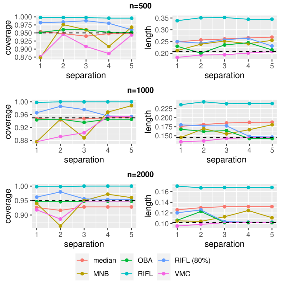
Figure C1: Low-dimensional prediction: coverage and length of $95\%$ CIs for $\beta^{*}=\theta^{*}_{1}$ with 8 majority sites and varying separation levels where $1$ is the lowest (hardest to detect) and $5$ is the highest (easiest to detect). “median” stands for the CI based on the median estimator, “MNB” stands for the m-out-of-n bootstrap CI in (38), “VMC” stands for the voting with maximum clique estimator and its associated CI in (10), “OBA” stands for the oracle bias aware CI in (39), “RIFL” stands for our proposed CI in (19), and “RIFL (80%)” stands for our proposed RIFL CI leveraging 80% rule. Results are based on 500 simulation replications. Dash lines in the left panels correspond to nominal coverage level 0.95; in the right panels correspond to the width of an oracle CI knowing the prevailing set.

Next, we present additional simulation results for the high-dimensional prediction example in Section 5.2 for $\theta_{11}^{*}$ with 8 majority sites. The simulation setup is the same as that in Section 6.2 except that $\theta^{(l)}=\theta^{*}$ for $l\in\{1,\ldots,8\}$ and $\theta_{j}^{(9)}=\theta_{j}^{*}+0.2+0.05a$ and $\theta_{j}^{(10)}=\theta_{j}^{*}+0.15+0.05a$ for $6\leq j\leq 11$ with $a$ varied in $\{1,2,3,4,5\}$ to represent varying levels of separation between the majority and non-majority sites. The results are presented in Figure C2, and we observe similar patterns as in the case with 6 majority sites. Simulation results for $\theta_{8}^{*}$ are presented in Figure C3 and Figure C4 for 6 and 8 majority sites, respectively. Again, we observe similar patterns as in the case for $\theta_{11}^{*}$.

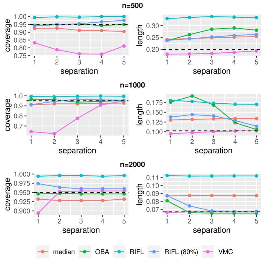
Figure C2: High-dimensional prediction: coverage and length of $95\%$ CIs for $\beta^{*}=\theta^{*}_{11}$ with 8 majority sites and varying separation levels where $1$ is the lowest (hardest to detect) and $5$ is the highest (easiest to detect). “median” stands for the CI based on the median estimator, “VMC” stands for the voting with maximum clique estimator and its associated CI in (10), “OBA” stands for the oracle bias aware CI in (39), “RIFL” stands for our proposed CI in (19), and “RIFL (80%)” stands for our proposed RIFL CI leveraging 80% rule. Results are based on 500 simulation replications. Dash lines in the left panels correspond to nominal coverage level 0.95; in the right panels correspond to the width of an oracle CI knowing the prevailing set.

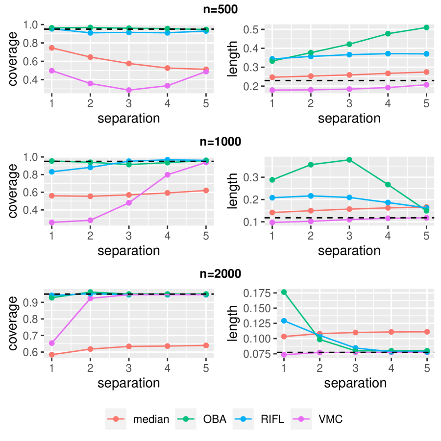
Figure C3: High-dimensional prediction: coverage and length of $95\%$ CIs for $\beta^{*}=\theta^{*}_{8}$ with 6 majority sites and varying separation levels where $1$ is the lowest (hardest to detect) and $5$ is the highest (easiest to detect). “median” stands for the CI based on the median estimator, “VMC” stands for the voting with maximum clique estimator and its associated CI in (10), “OBA” stands for the oracle bias aware CI in (39), “RIFL” stands for our proposed CI in (19), and “RIFL (80%)” stands for our proposed RIFL CI leveraging 80% rule. Results are based on 500 simulation replications. Dash lines in the left panels correspond to nominal coverage level 0.95; in the right panels correspond to the width of an oracle CI knowing the prevailing set.

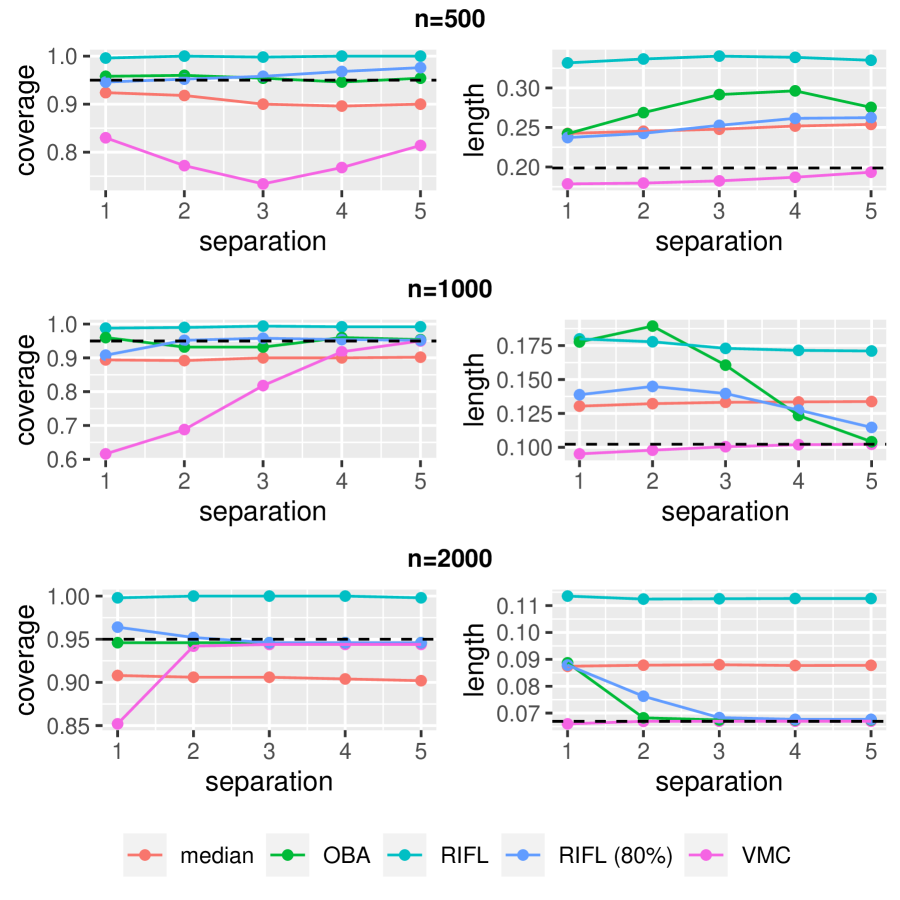
Figure C4: High-dimensional prediction: coverage and length of $95\%$ CIs for $\beta^{*}=\theta^{*}_{8}$ with 8 majority sites and varying separation levels where $1$ is the lowest (hardest to detect) and $5$ is the highest (easiest to detect). “median” stands for the CI based on the median estimator, “VMC” stands for the voting with maximum clique estimator and its associated CI in (10), “OBA” stands for the oracle bias aware CI in (39), “RIFL” stands for our proposed CI in (19), and “RIFL (80%)” stands for our proposed RIFL CI leveraging 80% rule. Results are based on 500 simulation replications. Dash lines in the left panels correspond to nominal coverage level 0.95; in the right panels correspond to the width of an oracle CI knowing the prevailing set.

Finally, we present results for the multi-source causal inference problem discussed in Sections 5.3 and 6.3 when there are 8 majority sites. Recall that the outcome for the $l$-th site is generated according to

$$Y_{i}^{(l)}=\mu_{l}+[X_{i}^{(l)}]^{\top}\zeta^{(l)}+\beta^{(l)}A_{i}^{(l)}+\varepsilon_{i}^{(l)},\quad\varepsilon_{i}^{(l)}\sim N(0,1).$$

For the case with 8 majority sites, we set $\beta^{(l)}=\beta^{*}=-1$ for $l\in\{1,2,\ldots,8\}$, $\beta^{(9)}=-1-0.2a$ and $\beta^{(10)}=-1-0.1a$, with $a$ varied in $\{1,2,3,4,5\}$. All the other aspects of the simulation setup is the same as that in Section 6.3. The results are summarized in Figure C5, and we again observe similar patterns.

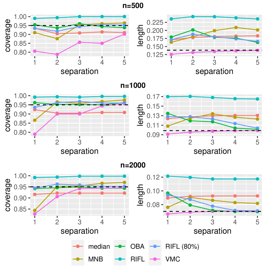
Figure C5: Causal inference: coverage and length of $95\%$ CIs for target ATE of the prevailing sites with 8 majority sites and varying separation levels where $1$ is the lowest (hardest to detect) and $5$ is the highest (easiest to detect). “median” stands for the CI based on the median estimator, “MNB” stands for the m-out-of-n bootstrap CI in (38), “VMC” stands for the voting with maximum clique estimator and its associated CI in (10), “OBA” stands for the oracle bias aware CI in (39), “RIFL” stands for our proposed CI in (19), and “RIFL (80%)” stands for our proposed RIFL CI leveraging 80% rule. Results are based on 500 simulation replications. Dash lines in the left panels correspond to nominal coverage level 0.95; in the right panels correspond to the width of an oracle CI knowing the prevailing set.

C.2 Choices of $\nu$ in m-out-of-n bootstrap

In this section, we present the empirical coverage and average length of the CIs obtained via m-out-of-n bootstrap with different choices of $m$. Specifically, we consider $m=n^{\nu}$ with $\nu$ varied in $\{0.6,0.7,0.8,0.9,1\}$. We focus on the low-dimensional prediction example in Section 6.1 with 6 majority sites and $n_{l}=1000$ for all 10 sites. All other simulation settings are the same as those described in Section 6.1.

The results are presented in Figure C6. We observe similar patterns in coverage for $\nu\in\{0.8,0.9,1\}$. Moreover, out of these 3 values, the choice of $\nu=0.8$ generally produces the shortest CI. For all choices of $\nu$, the MNB CI has coverage below nominal level when the separation level is low to moderate.

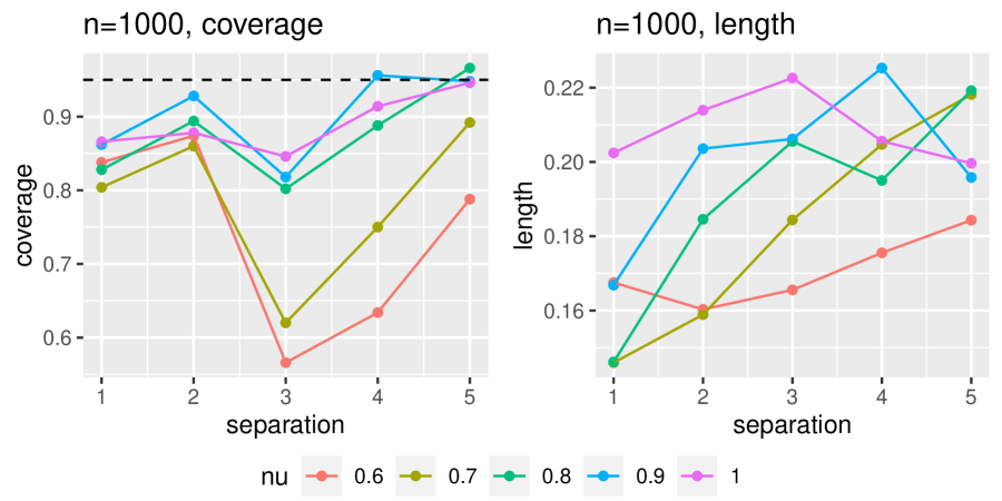
Figure C6: Low-dimensional prediction: coverage and length of $95\%$ CIs for $\beta^{*}=\theta^{*}_{1}$ of m-out-of-n bootstrap (MNB) CI with different choices of $m$. We set $m=n^{\nu}$ and vary $\nu$ in $\{0.6,0.7,0.8,0.9,1\}$. Sample size in each of the 10 sites is 1,000, and there are 6 majority sites. Results are based on 500 simulation replications. Dash lines in the left panels correspond to nominal coverage level 0.95.

C.3 Generalizability measure for the 16 sites in the real data analysis

In Figure C7, we present the full set of generalizability measure for all 16 sites in our Covid-19 real data analysis. Site 4 generally has lower generalizability than the other sites. When we focus on one specific risk factor (corresponding to one specific row of the plot in Figure C7), some sites have low generalizability, indicating that they may not belong to the prevailing set.

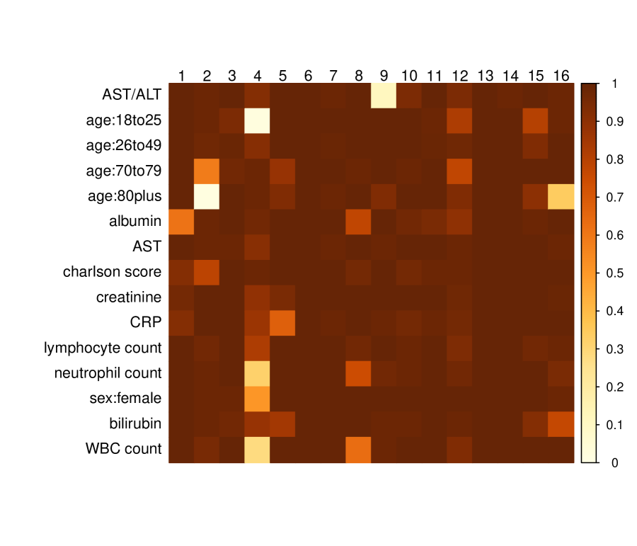
Figure C7: Generalizability measure for all 16 sites for each of the 15 risk factors. Each row corresponds to a risk factor and each column corresponds to a site.

References

• Andrews [2000] Donald WK Andrews. Inconsistency of the bootstrap when a parameter is on the boundary of the parameter space. Econometrica, pages 399–405, 2000.
• Arjovsky et al. [2019] Martin Arjovsky, Léon Bottou, Ishaan Gulrajani, and David Lopez-Paz. Invariant risk minimization. arXiv preprint arXiv:1907.02893, 2019.
• Armstrong et al. [2020] Timothy B Armstrong, Michal Kolesár, and Soonwoo Kwon. Bias-aware inference in regularized regression models. arXiv preprint arXiv:2012.14823, 2020.
• Bang and Robins [2005] Heejung Bang and James M Robins. Doubly robust estimation in missing data and causal inference models. Biometrics, 61(4):962–973, 2005.
• Belloni et al. [2014] Alexandre Belloni, Victor Chernozhukov, and Christian Hansen. Inference on treatment effects after selection among high-dimensional controls. The Review of Economic Studies, 81(2):608–650, 2014.
• Berk et al. [2013] Richard Berk, Lawrence Brown, Andreas Buja, Kai Zhang, and Linda Zhao. Valid post-selection inference. The Annals of Statistics, 41(2):802–837, 2013.
• Bickel and Sakov [2008] Peter J Bickel and Anat Sakov. On the choice of m in the m out of n bootstrap and confidence bounds for extrema. Statistica Sinica, pages 967–985, 2008.
• Bickel et al. [2009] Peter J Bickel, Ya’acov Ritov, and Alexandre B Tsybakov. Simultaneous analysis of lasso and dantzig selector. The Annals of statistics, 37(4):1705–1732, 2009.
• Bowden et al. [2016] Jack Bowden, George Davey Smith, Philip C Haycock, and Stephen Burgess. Consistent estimation in mendelian randomization with some invalid instruments using a weighted median estimator. Genetic epidemiology, 40(4):304–314, 2016.
• Brat et al. [2020] Gabriel A Brat, Griffin M Weber, Nils Gehlenborg, Paul Avillach, Nathan P Palmer, Luca Chiovato, James Cimino, Lemuel R Waitman, Gilbert S Omenn, Alberto Malovini, et al. International electronic health record-derived covid-19 clinical course profiles: the 4ce consortium. NPJ digital medicine, 3(1):1–9, 2020.
• Bühlmann and Meinshausen [2015] Peter Bühlmann and Nicolai Meinshausen. Magging: maximin aggregation for inhomogeneous large-scale data. Proceedings of the IEEE, 104(1):126–135, 2015.
• Bühlmann and van de Geer [2011] Peter Bühlmann and Sara van de Geer. Statistics for high-dimensional data: methods, theory and applications. Springer Science & Business Media, 2011.
• Burgess et al. [2017] Stephen Burgess, Dylan S Small, and Simon G Thompson. A review of instrumental variable estimators for mendelian randomization. Statistical methods in medical research, 26(5):2333–2355, 2017.
• Cai and Guo [2017] T Tony Cai and Zijian Guo. Confidence intervals for high-dimensional linear regression: Minimax rates and adaptivity. The Annals of statistics, 45(2):615–646, 2017.
• Cai and Guo [2020] T. Tony Cai and Zijian Guo. Semisupervised inference for explained variance in high dimensional linear regression and its applications. Journal of the Royal Statistical Society: Series B (Statistical Methodology), 82(2):391–419, 2020.
• Cai et al. [2021a] T Tony Cai, Zijian Guo, and Rong Ma. Statistical inference for high-dimensional generalized linear models with binary outcomes. Journal of the American Statistical Association, pages 1–14, 2021a.
• Cai et al. [2021b] Tianxi Cai, Molei Liu, and Yin Xia. Individual data protected integrative regression analysis of high-dimensional heterogeneous data. Journal of the American Statistical Association, pages 1–15, 2021b.
• Cai et al. [2021c] Tianxi Cai, T Tony Cai, and Zijian Guo. Optimal statistical inference for individualized treatment effects in high-dimensional models. Journal of the Royal Statistical Society: Series B (Statistical Methodology), 83(4):669–719, 2021c.
• Carraghan and Pardalos [1990] Randy Carraghan and Panos M Pardalos. An exact algorithm for the maximum clique problem. Operations Research Letters, 9(6):375–382, 1990.
• Chakraborty et al. [2013] Bibhas Chakraborty, Eric B Laber, and Yingqi Zhao. Inference for optimal dynamic treatment regimes using an adaptive m-out-of-n bootstrap scheme. Biometrics, 69(3):714–723, 2013.
• Chen and Xie [2014] Xueying Chen and Min-ge Xie. A split-and-conquer approach for analysis of extraordinarily large data. Statistica Sinica, pages 1655–1684, 2014.
• Chen et al. [2006] Yixin Chen, Guozhu Dong, Jiawei Han, Jian Pei, Benjamin W Wah, and Jianyong Wang. Regression cubes with lossless compression and aggregation. IEEE Transactions on Knowledge and Data Engineering, 18(12):1585–1599, 2006.
• Chernozhukov et al. [2015] Victor Chernozhukov, Christian Hansen, and Martin Spindler. Post-selection and post-regularization inference in linear models with many controls and instruments. 2015.
• Chodera et al. [2020] John Chodera, Alpha A Lee, Nir London, and Frank von Delft. Crowdsourcing drug discovery for pandemics. Nature Chemistry, 12(7):581–581, 2020.
• Davi et al. [2020] Ruthie Davi, Nirosha Mahendraratnam, Arnaub Chatterjee, C Jill Dawson, and Rachel Sherman. Informing single-arm clinical trials with external controls. Nature Reviews Drug Discovery, 19(12):821–822, 2020.
• Duan et al. [2020] Rui Duan, Chongliang Luo, Martijn J Schuemie, Jiayi Tong, C Jason Liang, Howard H Chang, Mary Regina Boland, Jiang Bian, Hua Xu, John H Holmes, et al. Learning from local to global: An efficient distributed algorithm for modeling time-to-event data. Journal of the American Medical Informatics Association, 27(7):1028–1036, 2020.
• Goyal et al. [2020] Parag Goyal, Justin J Choi, Laura C Pinheiro, Edward J Schenck, Ruijun Chen, Assem Jabri, Michael J Satlin, Thomas R Campion Jr, Musarrat Nahid, Joanna B Ringel, et al. Clinical characteristics of covid-19 in new york city. New England Journal of Medicine, 382(24):2372–2374, 2020.
• Guo [2020] Zijian Guo. Inference for high-dimensional maximin effects in heterogeneous regression models using a sampling approach. arXiv preprint arXiv:2011.07568, 2020.
• Guo [2021] Zijian Guo. Causal inference with invalid instruments: Post-selection problems and a solution using searching and sampling. arXiv preprint arXiv:2104.06911, 2021.
• Guo et al. [2018] Zijian Guo, Hyunseung Kang, T Tony Cai, and Dylan S Small. Confidence intervals for causal effects with invalid instruments by using two-stage hard thresholding with voting. Journal of the Royal Statistical Society: Series B (Statistical Methodology), 80(4):793–815, 2018.
• Guo et al. [2021a] Zijian Guo, Prabrisha Rakshit, Daniel S Herman, and Jinbo Chen. Inference for the case probability in high-dimensional logistic regression. The Journal of Machine Learning Research, 22(1):11480–11533, 2021a.
• Guo et al. [2021b] Zijian Guo, Claude Renaux, Peter Bühlmann, and Tony Cai. Group inference in high dimensions with applications to hierarchical testing. Electronic Journal of Statistics, 15(2):6633–6676, 2021b.
• Han et al. [2018] Larry Han, Angela Chen, Jason J Ong, Juliet Iwelunmor, and Joseph D Tucker. Crowdsourcing in health and health research: a practical guide. 2018.
• Han et al. [2021] Larry Han, Jue Hou, Kelly Cho, Rui Duan, and Tianxi Cai. Federated adaptive causal estimation (face) of target treatment effects. arXiv preprint arXiv:2112.09313, 2021.
• Hastie and Kameda [2005] Reid Hastie and Tatsuya Kameda. The robust beauty of majority rules in group decisions. Psychological review, 112(2):494, 2005.
• Heffernan and Heffernan [2014] Neil T Heffernan and Cristina Lindquist Heffernan. The assistments ecosystem: Building a platform that brings scientists and teachers together for minimally invasive research on human learning and teaching. International Journal of Artificial Intelligence in Education, 24(4):470–497, 2014.
• Hu et al. [2018] Weihua Hu, Gang Niu, Issei Sato, and Masashi Sugiyama. Does distributionally robust supervised learning give robust classifiers? In International Conference on Machine Learning, pages 2029–2037. PMLR, 2018.
• Jahanshahi et al. [2021] Mahta Jahanshahi, Keith Gregg, Gillian Davis, Adora Ndu, Veronica Miller, Jerry Vockley, Cecile Ollivier, Tanja Franolic, and Sharon Sakai. The use of external controls in fda regulatory decision making. Therapeutic Innovation & Regulatory Science, 55(5):1019–1035, 2021.
• Javanmard and Montanari [2014] Adel Javanmard and Andrea Montanari. Confidence intervals and hypothesis testing for high-dimensional regression. The Journal of Machine Learning Research, 15(1):2869–2909, 2014.
• Kang et al. [2016] Hyunseung Kang, Anru Zhang, T Tony Cai, and Dylan S Small. Instrumental variables estimation with some invalid instruments and its application to mendelian randomization. Journal of the American statistical Association, 111(513):132–144, 2016.
• Kang and Schafer [2007] Joseph DY Kang and Joseph L Schafer. Demystifying double robustness: A comparison of alternative strategies for estimating a population mean from incomplete data. Statistical science, 22(4):523–539, 2007.
• Kerr et al. [2004] Norbert L Kerr, R Scott Tindale, et al. Group performance and decision making. Annual review of psychology, 55(1):623–655, 2004.
• Keys et al. [2020] Kevin L Keys, Angel CY Mak, Marquitta J White, Walter L Eckalbar, Andrew W Dahl, Joel Mefford, Anna V Mikhaylova, María G Contreras, Jennifer R Elhawary, Celeste Eng, et al. On the cross-population generalizability of gene expression prediction models. PLoS genetics, 16(8):e1008927, 2020.
• Kraft et al. [2009] Peter Kraft, Eleftheria Zeggini, and John PA Ioannidis. Replication in genome-wide association studies. Statistical science: a review journal of the Institute of Mathematical Statistics, 24(4):561, 2009.
• Lee et al. [2016] Jason D Lee, Dennis L Sun, Yuekai Sun, and Jonathan E Taylor. Exact post-selection inference, with application to the lasso. Annals of Statistics, 44(3):907–927, 2016.
• Lee et al. [2017] Jason D Lee, Qiang Liu, Yuekai Sun, and Jonathan E Taylor. Communication-efficient sparse regression. The Journal of Machine Learning Research, 18(1):115–144, 2017.
• Leeb and Pötscher [2005] Hannes Leeb and Benedikt M Pötscher. Model selection and inference: Facts and fiction. Econometric Theory, pages 21–59, 2005.
• Leek et al. [2010] Jeffrey T Leek, Robert B Scharpf, Héctor Corrada Bravo, David Simcha, Benjamin Langmead, W Evan Johnson, Donald Geman, Keith Baggerly, and Rafael A Irizarry. Tackling the widespread and critical impact of batch effects in high-throughput data. Nature Reviews Genetics, 11(10):733–739, 2010.
• Li et al. [2013] Runze Li, Dennis KJ Lin, and Bing Li. Statistical inference in massive data sets. Applied Stochastic Models in Business and Industry, 29(5):399–409, 2013.
• Li et al. [2020] Sai Li, T Tony Cai, and Hongzhe Li. Transfer learning for high-dimensional linear regression: Prediction, estimation, and minimax optimality. arXiv preprint arXiv:2006.10593, 2020.
• Lian and Fan [2017] Heng Lian and Zengyan Fan. Divide-and-conquer for debiased l 1-norm support vector machine in ultra-high dimensions. The Journal of Machine Learning Research, 18(1):6691–6716, 2017.
• Ling et al. [2022] Wodan Ling, Jiuyao Lu, Ni Zhao, Anju Lulla, Anna M Plantinga, Weijia Fu, Angela Zhang, Hongjiao Liu, Hoseung Song, Zhigang Li, et al. Batch effects removal for microbiome data via conditional quantile regression. Nature Communications, 13(1):1–14, 2022.
• Liu et al. [2021] Molei Liu, Yin Xia, Kelly Cho, and Tianxi Cai. Integrative high dimensional multiple testing with heterogeneity under data sharing constraints. J. Mach. Learn. Res., 22:126–1, 2021.
• Maity et al. [2022] Subha Maity, Yuekai Sun, and Moulinath Banerjee. Meta-analysis of heterogeneous data: integrative sparse regression in high-dimensions. Journal of Machine Learning Research, 23(198):1–50, 2022.
• Mak et al. [2019] Raymond H Mak, Michael G Endres, Jin H Paik, Rinat A Sergeev, Hugo Aerts, Christopher L Williams, Karim R Lakhani, and Eva C Guinan. Use of crowd innovation to develop an artificial intelligence–based solution for radiation therapy targeting. JAMA oncology, 5(5):654–661, 2019.
• Meinshausen and Bühlmann [2015] Nicolai Meinshausen and Peter Bühlmann. Maximin effects in inhomogeneous large-scale data. The Annals of Statistics, 43(4):1801–1830, 2015.
• Ning and Liu [2017] Yang Ning and Han Liu. A general theory of hypothesis tests and confidence regions for sparse high dimensional models. The Annals of Statistics, 45(1):158–195, 2017.
• Peters et al. [2016] Jonas Peters, Peter Bühlmann, and Nicolai Meinshausen. Causal inference by using invariant prediction: identification and confidence intervals. Journal of the Royal Statistical Society: Series B (Statistical Methodology), 78(5):947–1012, 2016.
• Rasmy et al. [2018] Laila Rasmy, Yonghui Wu, Ningtao Wang, Xin Geng, W Jim Zheng, Fei Wang, Hulin Wu, Hua Xu, and Degui Zhi. A study of generalizability of recurrent neural network-based predictive models for heart failure onset risk using a large and heterogeneous ehr data set. Journal of biomedical informatics, 84:11–16, 2018.
• Rothenhäusler et al. [2016] Dominik Rothenhäusler, Nicolai Meinshausen, and Peter Bühlmann. Confidence intervals for maximin effects in inhomogeneous large-scale data. In Statistical Analysis for High-Dimensional Data, pages 255–277. Springer, 2016.
• Sagawa et al. [2019] Shiori Sagawa, Pang Wei Koh, Tatsunori B Hashimoto, and Percy Liang. Distributionally robust neural networks for group shifts: On the importance of regularization for worst-case generalization. arXiv preprint arXiv:1911.08731, 2019.
• Short et al. [2017] Ryan G Short, Dana Middleton, Nicholas T Befera, Raj Gondalia, and Tina D Tailor. Patient-centered radiology reporting: using online crowdsourcing to assess the effectiveness of a web-based interactive radiology report. Journal of the American College of Radiology, 14(11):1489–1497, 2017.
• Sorkin et al. [1998] Robert D Sorkin, Ryan West, and Donald E Robinson. Group performance depends on the majority rule. Psychological Science, 9(6):456–463, 1998.
• Surowiecki [2005] James Surowiecki. The wisdom of crowds. Anchor, 2005.
• Tao and Fu [2019] Yebin Tao and Haoda Fu. Doubly robust estimation of the weighted average treatment effect for a target population. Statistics in medicine, 38(3):315–325, 2019.
• Tian and Feng [2022] Ye Tian and Yang Feng. Transfer learning under high-dimensional generalized linear models. Journal of the American Statistical Association, (just-accepted):1–30, 2022.
• Tong et al. [2022] Jiayi Tong, Chongliang Luo, Md Nazmul Islam, Natalie E Sheils, John Buresh, Mackenzie Edmondson, Peter A Merkel, Ebbing Lautenbach, Rui Duan, and Yong Chen. Distributed learning for heterogeneous clinical data with application to integrating covid-19 data across 230 sites. NPJ digital medicine, 5(1):1–8, 2022.
• Trippa et al. [2015] Lorenzo Trippa, Levi Waldron, Curtis Huttenhower, and Giovanni Parmigiani. Bayesian nonparametric cross-study validation of prediction methods. The Annals of Applied Statistics, 9(1):402–428, 2015.
• Tsiatis [2006] Anastasios A Tsiatis. Semiparametric theory and missing data. 2006.
• Turcato et al. [2022] Gianni Turcato, Arian Zaboli, Irena Kostic, Barbara Melchioretto, Laura Ciccariello, Eleonora Zaccaria, Alessia Olivato, Antonio Maccagnani, Norbert Pfeifer, and Antonio Bonora. Severity of sars-cov-2 infection and albumin levels recorded at the first emergency department evaluation: a multicentre retrospective observational study. Emergency Medicine Journal, 39(1):63–69, 2022.
• van de Geer et al. [2014] Sara van de Geer, Peter Bühlmann, Ya’acov Ritov, and Ruben Dezeure. On asymptotically optimal confidence regions and tests for high-dimensional models. The Annals of Statistics, 42(3):1166–1202, 2014.
• Ventz et al. [2019] Steffen Ventz, Albert Lai, Timothy F Cloughesy, Patrick Y Wen, Lorenzo Trippa, and Brian M Alexander. Design and evaluation of an external control arm using prior clinical trials and real-world datadesign and evaluation of an external control arm. Clinical Cancer Research, 25(16):4993–5001, 2019.
• Vo et al. [2021] Thanh Vinh Vo, Trong Nghia Hoang, Young Lee, and Tze-Yun Leong. Federated estimation of causal effects from observational data. arXiv preprint arXiv:2106.00456, 2021.
• Wang et al. [2020] Cheng Wang, Larry Han, Gabriella Stein, Suzanne Day, Cedric Bien-Gund, Allison Mathews, Jason J Ong, Pei-Zhen Zhao, Shu-Fang Wei, Jennifer Walker, et al. Crowdsourcing in health and medical research: a systematic review. Infectious diseases of poverty, 9(1):1–9, 2020.
• Wang et al. [2021] Ruoyu Wang, Qihua Wang, and Wang Miao. A robust fusion-extraction procedure with summary statistics in the presence of biased sources. arXiv preprint arXiv:2108.12600, 2021.
• Wang et al. [2019] Xiaozhou Wang, Zhuoyi Yang, Xi Chen, and Weidong Liu. Distributed inference for linear support vector machine. Journal of Machine Learning Research, 20(113):1–41, 2019.
• Weber et al. [2022] Griffin M Weber, Chuan Hong, Zongqi Xia, Nathan P Palmer, Paul Avillach, Sehi L’Yi, Mark S Keller, Shawn N Murphy, Alba Gutiérrez-Sacristán, Clara-Lea Bonzel, et al. International comparisons of laboratory values from the 4ce collaborative to predict covid-19 mortality. NPJ digital medicine, 5(1):1–8, 2022.
• Windmeijer et al. [2019] Frank Windmeijer, Helmut Farbmacher, Neil Davies, and George Davey Smith. On the use of the lasso for instrumental variables estimation with some invalid instruments. Journal of the American Statistical Association, 114(527):1339–1350, 2019.
• Windmeijer et al. [2021] Frank Windmeijer, Xiaoran Liang, Fernando P Hartwig, and Jack Bowden. The confidence interval method for selecting valid instrumental variables. Journal of the Royal Statistical Society: Series B (Statistical Methodology), 83(4):752–776, 2021.
• Wu and McGoogan [2020] Zunyou Wu and Jennifer M McGoogan. Characteristics of and important lessons from the coronavirus disease 2019 (covid-19) outbreak in china: summary of a report of 72 314 cases from the chinese center for disease control and prevention. jama, 323(13):1239–1242, 2020.
• Wynants et al. [2020] Laure Wynants, Ben Van Calster, Gary S Collins, Richard D Riley, Georg Heinze, Ewoud Schuit, Marc MJ Bonten, Darren L Dahly, Johanna A Damen, Thomas PA Debray, et al. Prediction models for diagnosis and prognosis of covid-19: systematic review and critical appraisal. bmj, 369, 2020.
• Xie and Wang [2022] Min-ge Xie and Peng Wang. Repro samples method for finite-and large-sample inferences. arXiv preprint arXiv:2206.06421, 2022.
• Xiong et al. [2021] Ruoxuan Xiong, Allison Koenecke, Michael Powell, Zhu Shen, Joshua T Vogelstein, and Susan Athey. Federated causal inference in heterogeneous observational data. arXiv preprint arXiv:2107.11732, 2021.
• Zhang and Zhang [2014] Cun-Hui Zhang and Stephanie S Zhang. Confidence intervals for low dimensional parameters in high dimensional linear models. Journal of the Royal Statistical Society: Series B (Statistical Methodology), 76(1):217–242, 2014.
• Zhao et al. [2016] Tianqi Zhao, Guang Cheng, and Han Liu. A partially linear framework for massive heterogeneous data. Annals of statistics, 44(4):1400, 2016.
• Zhu and Bradic [2018] Yinchu Zhu and Jelena Bradic. Linear hypothesis testing in dense high-dimensional linear models. Journal of the American Statistical Association, 113(524):1583–1600, 2018.
• Zou [2006] Hui Zou. The adaptive lasso and its oracle properties. Journal of the American statistical association, 101(476):1418–1429, 2006.