Robust Consensus Clustering and its Applications for Advertising Forecasting

Abstract

Consensus clustering aggregates partitions in order to find a better fit by reconciling clustering results from different sources/executions. In practice, there exist noise and outliers in clustering task, which, however, may significantly degrade the performance. To address this issue, we propose a novel algorithm – robust consensus clustering that can find common ground truth among experts’ opinions, which tends to be minimally affected by the bias caused by the outliers. In particular, we formalize the robust consensus clustering problem as a constraint optimization problem, and then derive an effective algorithm upon alternating direction method of multipliers (ADMM) with rigorous convergence guarantee. Our method outperforms the baselines on benchmarks. We apply the proposed method to the real-world advertising campaign segmentation and forecasting tasks using the proposed consensus clustering results based on the similarity computed via Kolmogorov-Smirnov Statistics. The accurate clustering result is helpful for building the advertiser profiles so as to perform the forecasting.

Introduction

Consensus clustering reconciles clustering information from different sources (or different executions) to be better fit than the existing clustering results. The consensus clustering results, however can be biased due to different types of features, different executions of algorithms, different definitions of distance metrics and even different parameter settings, as is sharply observed by existing studies (?). All these factors may lead to disparity in clustering results. The major consensus clustering algorithms include Hypergraph partitioning (?),  (?), voting approach (?),  (?), mutual information  (?) (?), co-association approach (?), mixture model (?)  (?), correlation consensus (?), ensemble clustering (?),  (?),  (?),  (?), etc.

One key observation is that in consensus clustering  (?), if there exist noise and outliers in one source of features in any execution of algorithm, the clustering result might be significantly affected due to the least square loss function used in most of the clustering methods (such as k-means, Gaussian mixture model), because the errors are squared. Even worse, most of the time, the users have little prior knowledge of noise, which makes the clustering result more unstable and much harder to interpret with different initializations and parameter settings. For example, if one information source that we used for consensus clustering is not accurate, when we align the consensus clustering results against this “inaccurate” source, we will suffer from these inaccurate annotations. The inaccurate common characteristics extracted from the samples due to the biased clustering results, are in fact, however, less generalizable to those unseen ones.

To address these issues, this paper proposes a robust consensus clustering schema that is minimally affected by the outliers/noise. In particular, we combine multiple experts’ opinions on data clustering using the robust $\ell_{1}$-loss function that aims to find the maximum consistency on the experts’ opinions with minimum conflict. Our work can be viewed as an effective method of data clustering from heterogeneous information sources. The proposed method is practically feasible because it is independent of parameter settings of each clustering algorithm before aggregating the experts’ opinions. Driven by advertising applications, we apply the concensus clustering algorithm to cluster advertiser profiles (?) into different clusters so as to accurately perform performance (e.g.. Click, Conversions) forecasting.

The main contribution of this paper is summarized as follows.

• To address the issue of consensus clustering performance degradation in existence of noise and outliers, we rigorously formulate the problem of robust consensus clustering as an optimization problem using the robust loss function.

• To find the best solution for robust consensus clustering, we develop an effective algorithm upon ADMM to derive the optimal solution, whose convergence can be rigorously proved.

• We experimentally evaluate our proposed method on both benchmarks and real-world advertiser segmentation and forecasting tasks, and show that our method is effective and efficient in producing the better clustering results. As an application, the proposed algorithm is applied for advertising forecasting tasks with more stable and trustful solutions.

Robust consensus clustering Model

Problem setting Assume we have $n$ data points, each data point can generate features from different views (total view number=V). For example, an image can generate features using different descriptors, such as SIFT, HOG, CNN features (?). More formally, let $\mathbf{x}_{i}^{v}\in\Re^{p_{v}}$ be $v$-th ($1\leq v\leq V$) view/modal feature of a data point $i$, $p_{v}$ is the dimensionality of feature extracted from $v$-th view. Consider all data points,

$${\mathbf{X}}^{v}=[\mathbf{x}_{1}^{v},\mathbf{x}^{v}_{2},\cdots,\mathbf{x}^{v}_{n}],$$

where each data column vector is $\mathbf{x}^{v}_{i}\in\Re^{p_{v}\times 1}$. Each data point has the ground-truth label $y_{i}\in\Re^{K}$. Simple concatenation of all data views gives

$${\mathbf{X}}=\left[\begin{array}[]{c}{\mathbf{X}}^{1}\\ {\mathbf{X}}^{2}\\ \vdots\\ {\mathbf{X}}^{V}\\ \end{array}\right]=[\mathbf{x}_{1},\mathbf{x}_{2},\cdots,\mathbf{x}_{n}],\quad\mathbf{x}_{i}=\left(\begin{array}[]{c}\mathbf{x}^{1}_{i}\\ \mathbf{x}^{2}_{i}\\ \vdots\\ \mathbf{x}^{V}_{i}\\ \end{array}\right).$$

Suppose we are given the clustering/partition results (${\cal{P}}$) for data points $\{{\mathbf{X}}^{1},{\mathbf{X}}^{2},\cdots,{\mathbf{X}}^{V}\}$ from $V$ different views, i.e., ${\cal{P}}=\{\mathbf{G}^{1},\mathbf{G}^{2},\cdots,\mathbf{G}^{V}\}$, where $\mathbf{G}^{v}\in\{0,1\}^{n\times K}$ (for K clusters) is the clustering result from view $v$. The clusters/partitions assignment might be different for different views. Let the connectivity matrix (a.k.a co-association matrix) ${\mathbf{M}}\in\{0,1\}^{n\times n}$, where $M_{ij}(\mathbf{G}^{V})$ for view $v$ between data point $i,j$ is:

$$M_{ij}(\mathbf{G}^{v})=\left\{{\begin{array}[]{*{20}c}{1;\;\;\text{{\kern 1.0pt} {\kern 1.0pt} {\kern 1.0pt} (i,j){\kern 1.0pt} {\kern 1.0pt} belongs{\kern 1.0pt} {\kern 1.0pt} {\kern 1.0pt} to{\kern 1.0pt} {\kern 1.0pt} {\kern 1.0pt} the{\kern 1.0pt} {\kern 1.0pt} same{\kern 1.0pt} {\kern 1.0pt} {\kern 1.0pt} clustering}}\\ {0.\;\;\;\;\;\;\;\;\;\;\;\;\;\;\;\;\;\;\;\;\;\;\;\;\;\;\;\;\;\;\;\;\;\;\;\;\;\;\;\;\;\;\;\;\text{otherwise}}\\ \end{array}}\right.$$ (3)

Co-association consensus clustering

Standard consensus clustering looks for a consensus clustering (based on majority agreement) $\mathbf{G}^{*}\in\{0,1\}^{n\times K}$, such that $\mathbf{G}^{*}$ is closest to the all the given partitions, i.e.,

$$\min_{\mathbf{G}^{*}}J(\mathbf{G}^{*})=\frac{1}{V}\sum_{v=1}^{V}\sum_{i=1}^{n}\sum_{j=1}^{n}D(M_{ij}(\mathbf{G}^{v})-M_{ij}(\mathbf{G}^{*})),$$ (4)

where $D(.)$ is a distance function between the optimal solution and the solution from each view. Generally, least square loss is used for function $D(.)$:

$$\min_{\mathbf{G}^{*}}J(\mathbf{G}^{*})=\frac{1}{V}\sum_{v=1}^{V}\sum_{i=1}^{n}\sum_{j=1}^{n}\Big{(}M_{ij}(\mathbf{G}^{v})-M_{ij}(\mathbf{G}^{*})\Big{)}^{2},$$ (5)

Notice that $M_{ij}(\mathbf{G}^{v})={0,1}$, therefore, Eq.(5) can be equivalently written as:

$$\min_{\mathbf{G}^{*}}J_{2}(\mathbf{G}^{*})=\frac{1}{V}\sum_{v=1}^{V}\sum_{i=1}^{n}\sum_{j=1}^{n}|M_{ij}(\mathbf{G}^{v})-M_{ij}(\mathbf{G}^{*})|$$

$$=\frac{1}{V}\sum_{v=1}^{V}\|M(\mathbf{G}^{v})-M(\mathbf{G}^{*})\|_{1},$$ (6)

with $\|X\|_{1}:=\sum_{i,j}|X_{ij}|$.

Let

$$\mathbf{G}_{\ell_{2}}=\operatorname*{arg\,min}_{\mathbf{G}^{*}}J(\mathbf{G}^{*})$$ (7)

$$\mathbf{G}_{\ell_{1}}=\operatorname*{arg\,min}_{\mathbf{G}^{*}}J_{2}(\mathbf{G}^{*}).$$ (8)

Clearly,

$$\mathbf{G}_{\ell_{2}}=\mathbf{G}_{\ell_{1}}.$$ (9)

Analysis Given little (or no) prior information of clustering result from each view, one natural way to compute the associate between data points $i$ and $j$ is to get the expected value of average association $\tilde{M}=[\tilde{M}_{ij}]$, i.e.,

$$\tilde{M}_{ij}=\frac{1}{V}\sum_{v=1}^{V}M_{ij}(\mathbf{G}^{v}).$$ (10)

Back to model of Eq.(Co-association consensus clustering), the upper bound of $J_{2}$ is given by:

$$J_{2}\leq\frac{1}{V}\sum_{v=1}^{V}\|{\mathbf{M}}(\mathbf{G}^{v})-\tilde{{\mathbf{M}}}\|_{1}+\|\tilde{{\mathbf{M}}}-{\mathbf{M}}(\mathbf{G}^{*})\|_{1}$$

$$=C+\|\tilde{{\mathbf{M}}}-{\mathbf{M}}(\mathbf{G}^{*})\|_{1}$$

$$=C+J_{3}(\mathbf{G}^{*})$$ (11)

where

$$J_{3}(\mathbf{G}^{*})=\|\tilde{{\mathbf{M}}}-{\mathbf{M}}(\mathbf{G}^{*})\|_{1}$$ (12)

$$C=\frac{1}{V}\sum_{v=1}^{V}\|{\mathbf{M}}(\mathbf{G}^{v})-\tilde{{\mathbf{M}}}\|_{1}$$ (13)

Note the first term is a constant $C$ because it measures the average difference between the final clustering assignment and the average consensus association $\tilde{{\mathbf{M}}}$. The smaller value of this term gives the closer distance between the final clustering assignment and current partition from a specific view.

On the other hand,

$$J_{3}\leq\frac{1}{V}\sum_{v=1}^{V}\Big{(}\|{\mathbf{M}}(\mathbf{G}^{v})-{\mathbf{M}}(\mathbf{G}^{*})\|_{1}+\|\tilde{{\mathbf{M}}}-{\mathbf{M}}(\mathbf{G}^{v})\|_{1}\Big{)}$$

$$=J_{2}(\mathbf{G}^{*})+C$$ (14)

This analysis indicates that the optimization of $J_{2}$ can be achieved by $J_{3}$.

Clustering indicator One way to optimize $J_{3}$ of $\|\tilde{{\mathbf{M}}}-{\mathbf{M}}(\mathbf{G}^{*})\|_{1}$ of Eq.(12) is to assign the optimal clustering indicator $\mathbf{G}\in\{0,1\}^{n\times K}$, with the constraint that $\sum_{k}G_{ik}=1$, i.e., there is only one ‘1’ in each row of $\mathbf{G}$, and the rest are zeros. The connection between the averaged connectivity matrix ${\mathbf{M}}(\mathbf{G}^{*})$ and $\mathbf{G}$ is:

$${\mathbf{M}}(\mathbf{G}^{*})=\mathbf{G}^{*}\mathbf{G}^{*{\intercal}}.$$ (15)

Therefore the objective of Eq.(12) becomes $J_{4}$, i.e.,

$$\min_{\mathbf{G}}J_{4}(\mathbf{G})=\|\tilde{{\mathbf{M}}}-\mathbf{G}\mathbf{G}^{\intercal}\|_{1}$$

$$\;\;s.t.,\;\;\;\mathbf{G}\in\{0,1\}^{n\times K},\;\;\sum_{k}G_{ik}=1$$ (16)

Relaxation in continuous domain

However, the major difficulty of solving Eq.(16) is that is involves the discrete clustering indicator $\mathbf{G}$ and the algorithm is NP-complete (?). Also the objective involves non-smooth $\ell_{1}$ norm, which generally, is hard to handle. Thus, as most of the spectral clustering solvers, we do normalization on cluster indicators. In particular, we use ${\mathbf{H}}\in\Re^{n\times K}$ to denote the new clustering indicator, i.e.,

$${\mathbf{H}}=\mathbf{G}(\mathbf{G}^{\intercal}\mathbf{G})^{-\frac{1}{2}}.$$

Notice that

$$\mathbf{G}^{\intercal}\mathbf{G}=\left({\begin{array}[]{*{20}c}{n_{1}}&{}\hfil&{}\hfil&{}\hfil&{}\hfil\\ {}\hfil&{n_{2}}&{}\hfil&{}\hfil&{}\hfil\\ {}\hfil&{}\hfil&{...}&{}\hfil&{}\hfil\\ {}\hfil&{}\hfil&{}\hfil&{...}&{}\hfil\\ {}\hfil&{}\hfil&{}\hfil&{}\hfil&{n_{k}}\\ \end{array}}\right),$$ (22)

where $n_{k}$ is the number of data points that falls in category $k$. Let diagonal matrix $\mathbf{D}\in\Re^{k\times k}$, i.e.,

$$\mathbf{D}:=\mathbf{G}^{\intercal}\mathbf{G}.$$

then

$$\mathbf{G}\mathbf{G}^{\intercal}={\mathbf{H}}\mathbf{D}{\mathbf{H}}^{\intercal};$$ (23)

$${\mathbf{H}}^{\intercal}{\mathbf{H}}=\mathbf{G}(\mathbf{G}^{\intercal}\mathbf{G})^{-1}={\mathbf{I}}_{k},$$ (24)

where ${\mathbf{I}}_{k}$ is an identity matrix with size kxk. Therefore the objective function to be solved becomes:

$$\min_{{\mathbf{H}},\mathbf{D}}J_{5}({\mathbf{H}},\mathbf{D})=\|\tilde{{\mathbf{M}}}-{\mathbf{H}}\mathbf{D}{\mathbf{H}}^{\intercal}\|_{1}\;\;$$

$$s.t.,\;\;\;{\mathbf{H}}^{\intercal}{\mathbf{H}}={\mathbf{I}}_{K},\;\;\mathbf{D}\geq 0;\;\;\mathbf{D}\;\;\text{is diagonal},$$ (25)

where $\mathbf{G}={\mathbf{H}}\mathbf{D}^{{\frac{1}{2}}}$ can be obtained in continous domain.

In practice, the solution obtained from $\hat{{\mathbf{M}}}$ may not be accurate due to noise or outliers. For this reason, we term our method as “robust” because we use $\ell_{1}$ distance to measure the differences between the consensus optimal solution and the solution computed from each view. The errors are not squared. Therefore, our model is capable of handling any noises/outliers in some view/execution in data clustering.

Further, we have:

Lemma 1

Set $\hat{{\mathbf{M}}}$ to be the normalized pairwise similarity matrix $\hat{\SS}=\mathbf{D}^{-{\frac{1}{2}}}\SS\mathbf{D}^{-{\frac{1}{2}}}$ ($\SS\in\Re^{n\times n}$ and $S_{ij}$ is the similarity between data point $i$ and $j$), using robust $\ell_{1}$-norm as the loss function, i.e.,

$$\min_{{\mathbf{H}}}J_{0}({\mathbf{H}})=\|\hat{\SS}-{\mathbf{H}}{\mathbf{H}}^{\intercal}\|_{F}^{2}$$

$$\;\;s.t.,\;\;\;{\mathbf{H}}^{\intercal}{\mathbf{H}}={\mathbf{I}}_{k}.$$ (26)

This is identical to normalized cut spectral clustering (?).

Proof Recall that in standard normalized cut spectral clustering, the objective is:

$$\min_{{\mathbf{H}}}{\mbox{Tr}}({\mathbf{H}}^{\intercal}({\mathbf{I}}-\hat{\SS}){\mathbf{H}})$$

$$\;\;s.t.,\;\;\;{\mathbf{H}}^{\intercal}{\mathbf{H}}={\mathbf{I}}_{k},$$ (27)

where $\hat{\SS}=\mathbf{D}^{-{\frac{1}{2}}}\SS\mathbf{D}^{-{\frac{1}{2}}}$. This is equivalent to optimizing:

$$\max_{{\mathbf{H}}}{\mbox{Tr}}({\mathbf{H}}^{\intercal}\hat{\SS}{\mathbf{H}})$$

$$\;\;s.t.,\;\;\;{\mathbf{H}}^{\intercal}{\mathbf{H}}={\mathbf{I}}_{k}.$$ (28)

Notice that

$$\|\hat{\SS}-{\mathbf{H}}{\mathbf{H}}^{\intercal}\|_{F}^{2}={\mbox{Tr}}(\hat{\SS}^{\intercal}\hat{\SS}+{\mathbf{H}}{\mathbf{H}}^{\intercal}{\mathbf{H}}^{\intercal}{\mathbf{H}}-2\hat{\SS}^{\intercal}{\mathbf{H}}{\mathbf{H}}^{\intercal}),$$

${\mbox{Tr}}({\mathbf{H}}{\mathbf{H}}^{\intercal}{\mathbf{H}}^{\intercal}{\mathbf{H}})=\text{const}$, and therefore $\min_{{\mathbf{H}}}\|\hat{\SS}-{\mathbf{H}}{\mathbf{H}}^{\intercal}\|_{F}^{2}$ is equivalent to $\max_{{\mathbf{H}}}{\mbox{Tr}}({\mathbf{H}}^{\intercal}\hat{\SS}{\mathbf{H}})$. This completes the proof.

In this paper next, we discuss how to solve the robust consensus clustering model of Eq.(Relaxation in continuous domain).

Optimization Algorithm

Eq.(Relaxation in continuous domain) seems difficult to solve since it involves non-smooth loss and high-order matrix optimization. We show how to apply alternating direction method of multipliers (ADMM) to solve it. ADMM method decomposes a large optimization problem by breaking them into smaller pieces, each of which are then easier to handle. ADMM combines the benefits of dual decomposition and augmented Lagrangian method for constrained optimization problem (?) and has been applied in many applications. The problem solved by ADMM method usually has the following general forms, i.e.,

$$\min_{{\mathbf{X}},{\mathbf{Z}}}f({\mathbf{X}})+g({\mathbf{Z}}),\;\;\;s.t.\quad\quad{\mathbf{A}}{\mathbf{X}}+\mathbf{B}{\mathbf{Z}}={\mathbf{C}}$$ (29)

After enforcing the Lagrangian multiplier while introducing more variables, the problem can be solved alternatively, i.e.,

$$\ell({\mathbf{X}},{\mathbf{Z}},\mu)=f({\mathbf{X}})+g({\mathbf{Z}})+\Omega^{\top}({\mathbf{A}}{\mathbf{X}}+\mathbf{B}{\mathbf{Z}}-{\mathbf{C}})$$

$$+\frac{\mu}{2}||{\mathbf{A}}{\mathbf{X}}+\mathbf{B}{\mathbf{Z}}-{\mathbf{C}}||_{F}^{2},$$ (30)

$${{\mathbf{X}}}^{t+1}:=\operatorname*{arg\,min}_{{\mathbf{X}}}{\ell({\mathbf{X}},{\mathbf{Z}}^{t},\mu^{t})},$$

$${{\mathbf{Z}}}^{t+1}:=\operatorname*{arg\,min}_{{\mathbf{Z}}}{\ell({\mathbf{X}}^{t+1},{\mathbf{Z}},\mu^{t})},$$

$${\Omega}^{t+1}:={\Omega}^{t}+\mu{({\mathbf{A}}{\mathbf{X}}^{t+1}+\mathbf{B}{\mathbf{X}}^{t+1}-{\mathbf{C}})}.$$

and $\Omega$ is the augmented Lagrangian multiplier, and $\mu$ is the non-negative step size.

Optimization Algorithm to solve Eq.(Relaxation in continuous domain)

According to ADMM algorithm, by imposing constraint variable

$${\mathbf{E}}={\tilde{\mathbf{M}}}-{\mathbf{H}}\mathbf{D}{\mathbf{H}}^{{}^{\intercal}},$$

the problem of Eq.(Relaxation in continuous domain) is equivalent to solving,

$$\min_{{\mathbf{E}},\;{\mathbf{H}},\;\mathbf{D}}\|{\mathbf{E}}\|_{1},$$

$$s.t.\quad\quad{\mathbf{E}}-({\tilde{\mathbf{M}}}-{\mathbf{H}}\mathbf{D}{\mathbf{H}}^{\intercal})=0;$$

$$s.t.,{\mathbf{H}}^{{}^{\intercal}}{\tilde{\mathbf{H}}}={\mathbf{I}}_{K},\;\;\mathbf{D}\geq 0;\;\;\mathbf{D}\;\;\text{is diagonal}$$ (31)

In ADMM algorithm, to solve $f({\mathbf{E}})=\|{\mathbf{E}}\|_{1}$, under the constraint

$$h({\mathbf{E}})={\mathbf{E}}-({\tilde{\mathbf{M}}}-{\mathbf{H}}\mathbf{D}{\mathbf{H}}^{T}),$$

the ADMM function can be formulated as follows,

$$\ell({\mathbf{E}},{\mathbf{H}},\mathbf{D},\Omega,\mu)=f({\mathbf{E}})+\Omega^{\top}h({\mathbf{E}})+\frac{\mu}{2}||h({\mathbf{E}})||_{F}^{2}.$$

where Lagrange multiplier is $\Omega$ and $\mu$ is the penalty constant. We solve a sequence of subproblems

$$\min_{{\mathbf{E}},{\mathbf{H}},\mathbf{D}}\|{\mathbf{E}}\|_{1}+\Omega^{{}^{\top}}({\mathbf{E}}-({\tilde{\mathbf{M}}}-{\mathbf{H}}\mathbf{D}{\mathbf{H}}^{{}^{\intercal}}))$$

$$+\frac{\mu}{2}\|{\mathbf{E}}-({\tilde{\mathbf{M}}}-{\mathbf{H}}\mathbf{D}{\mathbf{H}}^{{}^{\intercal}})\|_{F}^{2}.$$ (32)

with $\Omega$ and $\mu$ updated in a specified pattern:

$$\Omega\leftarrow\Omega+\mu({\mathbf{E}}-({\tilde{\mathbf{M}}}-{\mathbf{H}}\mathbf{D}{\mathbf{H}}^{{}^{\intercal}})),$$

$$\mu\leftarrow\rho\mu.$$

To solve Eq.(Optimization Algorithm to solve Eq.()), we search for optimal ${\mathbf{E}}$, ${\mathbf{H}},\mathbf{D}$ iteratively until the algorithm converges. Now we discuss how to solve ${\mathbf{E}}$, ${\mathbf{H}}$, $\mathbf{D}$ in each step. Alg.1 summarizes the complete algorithm.

Algorithm 1 Solving robust consensus clustering model of Eq.(Relaxation in continuous domain)

Input: clustering results from different views ${\tilde{\mathbf{M}}}$, parameter $\rho>1$.
  Output: final clustering indicator ${\mathbf{H}}$.
  Procedure:

1:  Initialize ${\mathbf{E}}^{0}$, ${\mathbf{H}}^{0},\mathbf{D}^{0}$, $\Omega^{0}$, $\mu^{0}>0$, $t=0$

2:  while Not converge  do

3:     Update ${\mathbf{E}}$ via Eq.(34)

4:     Update ${\mathbf{H}}$ via Eq.(36)

5:     Update $\mathbf{D}$ via Eq.(37)

6:     $\mu^{t+1}:=\rho\mu^{t}$

7:     $\Omega:=\Omega+\mu({\mathbf{E}}-({\tilde{\mathbf{M}}}-{\mathbf{H}}\mathbf{D}{\mathbf{H}}^{{}^{\intercal}}))$

8:     $t:=t+1$

9:  end while

Update ${\mathbf{E}}$

To update the error matrix ${\mathbf{E}}$, we derive Eq.(33) with fixed ${\mathbf{H}},\mathbf{D}$ and obtain the following form:

$$\min_{{\mathbf{E}}}\ \frac{\mu}{2}||{\mathbf{E}}-{\mathbf{A}}||_{F}^{2}+||{\mathbf{E}}||_{1}$$ (33)

where

$${\mathbf{A}}={\mathbf{H}}\mathbf{D}{\mathbf{H}}^{T}-{\tilde{\mathbf{M}}}+\frac{\Omega}{\mu},$$

It is well-known that the solution to the above LASSO type problem (?) is given by

$${\mathbf{E}}_{ij}=sign({\mathbf{A}}_{ij})\max(|{\mathbf{A}}_{ij}|-\frac{1}{\mu},0).$$ (34)

Update ${\mathbf{H}},\mathbf{D}$

To update ${\mathbf{H}},\mathbf{D}$ while fixing ${\mathbf{E}}$, we minimize the relevant part of Eq.(Optimization Algorithm to solve Eq.()) which is

$$\min_{{\mathbf{H}},\mathbf{D}}\frac{\mu}{2}\|\mathbf{B}-{\mathbf{H}}\mathbf{D}{\mathbf{H}}^{T}\|_{F}^{2},$$ (35)

$$s.t.,{\mathbf{H}}^{T}{\mathbf{H}}={\mathbf{I}}_{K},\;\;\mathbf{D}\geq 0;\;\;\mathbf{D}\;\;\text{is diagonal}$$

where

$$\mathbf{B}={\tilde{\mathbf{M}}}-{\mathbf{E}}+\frac{\Omega}{\mu}.$$

It is easy to see the optimal solution ${\mathbf{H}}$ is given by the $k$-largest eigenvectors of $\mathbf{B}$, i.e., ${\mathbf{H}}=[\mathbf{h}_{1},\mathbf{h}_{2},\cdot\cdot\cdot,\mathbf{h}_{k}]$,

$$\mathbf{B}\mathbf{h}_{k}=\lambda_{k}\mathbf{h}_{k},$$ (36)

where $\lambda_{k}$ is the associated eigen-value with respect to eigen-vector $\mathbf{h}_{k}$, and $\Lambda$ is a diagonal matrix, and

$$\Lambda=diag([\lambda_{1},\lambda_{2},\cdot\cdot\cdot,\lambda_{k}]).$$

Then the optimal solution of $\mathbf{D}$ is given by

$$\mathbf{D}=\Lambda.$$ (37)

The completes the algorithm for solving Eq.(Relaxation in continuous domain).

Time Complexity Analysis Since Eq.(Relaxation in continuous domain) is not a convex problem, in each iteration, given $\mu$, $\Sigma$, $\rho$, the algorithm will find its local solution. The convergence of ADMM algorithm has been proved and widely discussed in  (?).

The overall time cost for the algorithm depends on iterations and time cost for each variable updating. The computation of ${\mathbf{E}}$ takes ${\cal O}(nk^{2})$ time. The major burden is from the updating of $\mathbf{D}$ and ${\mathbf{H}}$, which requires computation of top $k$ eigen-vector of $\mathbf{B}$,i.e., ${\cal O}(n^{3})$ time. Overall, the cost of the algorithm 1 is ${\cal O}(T(n^{3}+nk^{2}))$, where $T$ is the iteration number before convergence. To make the solution scalable for large-scale dataset, We can accelerate this via Hessenberg reduction and QR iteration with multi-thread solver using GPU acceleration (?) and also use divide-and-conquer (?) to accelerate the execution.

Experimental Results on Benchmarks

Table 1: dataset descriptions

datasets	#data points	# feature	#class
CSTR	475	1000	4
Glass	214	9	7
Ionosphere	351	34	2
Iris	150	4	3
Reuters	2900	1000	10
Soybean	47	35	4
Wine	178	13	3
Zoo	101	18	7

Table 2: Accuracy on 8 benchmark datasets

datasets	k-means	KC	CSPA	HPGA	NMFC	WC	L2CC	RCC (our method)	ES	CorC
CSTR	0.45	0.38	0.50	0.62	0.56	0.64	0.61	0.65	0.64	0.61
Glass	0.38	0.45	0.43	0.40	0.49	0.49	0.49	0.52	0.52	0.50
Ionosphere	0.70	0.71	0.68	0.52	0.71	0.71	0.71	0.72	0.71	0.70
Iris	0.83	0.72	0.86	0.69	0.89	0.89	0.86	0.89	0.88	0.86
Reuters	0.45	0.44	0.43	0.44	0.43	0.44	0.43	0.45	0.44	0.43
Soybean	0.72	0.82	0.70	0.81	0.89	0.91	0.76	1.00	0.98	0.95
Wine	0.68	0.68	0.69	0.52	0.70	0.72	0.65	0.96	0.84	0.89
Zoo	0.61	0.59	0.56	0.58	0.62	0.70	0.80	0.84	0.79	0.82

Table 3: Clustering accuracy on three multi-view datasets

datasets	LBP	HOG	GIST	Classemes	FC	MVKmean	AP	LCC	RCC (Our method)
MSRC-v1	0.4731	0.6367	0.6283	0.5431	0.7423	0.7871	0.5369	0.7542	0.8017
Caltech-7	0.5236	0.5561	0.5473	0.4983	0.6123	0.6640	0.5359	0.6643	0.6819
Caltech-20	0.3378	0.3679	0.3925	0.3660	0.5489	0.5619	0.3421	0.6287	0.6374

In order to validate the effectiveness of our method, we perform experiments on benchmark datasets. In particular, we use six datasets downloaded from UCI machine learning repository, including Glass, Ionosphere, Iris, Soybean, Wine, zoo. We also adopted two widely used text datasets for document clustering, including CSTR and Reuters. The features we adopt are represented using vector space model after removing the stop words and unnecessary tags and headers. In Reuter dataset, we use the ten most frequent categories.

In our experiment, the consensus co-association matrix is obtained by running k-means algorithm for 40 times and make an average of results using different initializations. All datasets have the ground-truth of clustering labels. We also compare against the following baseline methods:

• k-means on original feature space

• KC: k-means on the consensus similarity matrix;

• NMFCC (?): NMF-based consensus clustering;

• CSPA (?): cluster based similarity partition algorithm

• HPGA (?): Hypergraph partitioning algorithm

• WCC (?): weighted consensus clustering

• L2CC: using standard $\ell_{2}$ loss for solving the consensus clustering on the consensus matrix;

• RCC: proposed robust consensus clustering algorithm

• Correlation Consensus (CorC) (?): Correlation based consensus clustering by exploiting the ranking of different views;

• Ensemble Consensus(ES) (?): ensemble consensus via exploiting Kullback-Leibler divergence of different aspects.

Evaluation metrics As the other clustering tasks, we use the clustering accuracy as the metric to evaluate the performance of our algorithms. Clustering accuracy(ACC) is defined as,

$$ACC=\frac{{\sum\nolimits_{i=1}^{n}{\delta({l_{i}},map({c_{i}}))}}}{n},$$ (38)

where $l_{i}$ is the true class label and $c_{i}$ is the obtained cluster label of $x_{i}$, map(.) is the best mapping function, $\delta(x,y)$ is the delta function where $\delta(x,y)=1$ if $x=y$, and $\delta(x,y)=0$ otherwise. The mapping function map(.) matches the true class label and the obtained clustering label, where the best mapping is solved by Hungarian algorithm. The larger, the better.

Experiment result analysis We report clustering results in Table. 2. Clearly, our method is very robust and outperforms the other methods. The accuracy gain is very significant especially on dataset Soybean, Wine and zoo. In some cases, the clustering result from one execution might be severely biased. This can be addressed by running clustering multiple times to reduce the variance. The Correlation Consensus algorithm (?) is designed for multi-modal data, which did not show very promising performance for the multiple execution of datasets with different initializations.

Experiment results on multi-view datasets

Dataset Our algorithm can be easily extended for processing multi-view data when $\tilde{{\mathbf{M}}}$ of Eq.(Relaxation in continuous domain) is computed using multi-view features. We evaluate this over several public datasets: Caltech101 (?) and Microsoft Research Cambridge Volume 1 (MSRCV1) (?). MSRCV1 has images from 7 classes, i.e., airplane, bicycle, building, car, cow, face, and tree. Each class has 30 images. Caltech-101 is an image dataset of 8677 images and 101 object classes. We follow the same experimental procedure as (?) and extract 7 and 20 classes for each experimental setup. We extract 1984-dimensional LBP (?) features, 4000-dimensional GIST (?) features, 768-dimensional HOG (?) features, 2659-dimensional classemes (?) features from each image.

Comparison results We compare our methods against clustering using each view of features, i.e., LBP, HOG, GIST and Classemes, respectively. We also compare several multi-view clustering methods: Spectral clustering using simple multi-view feature concatenation (denoted as FC), multi-view k-means (denoted as MVKmean) (?), affinity propagation using multi-view features ( denoted as AP) (?), low-rank consensus clustering (denoted as LCC) (?). Table. 3 presents the clustering accuracy results, which demonstrates the superiority of using our method for solving multi-view clusering problems. Moreover, our method is flexible for incorporating any view of features after properly feature extraction. Essentially, our method learns the low-rank subspace using eigen-decomposition using co-association matrix from multi-view data, which plays the similar role as those in (?),  (?).

Applications in Advertising Segmentation

Computational Advertising refers to serving the most relevant advertisement (ads for short) matching to the particular context in internet webs. One import problem is to segment advertisers into different segmentations and provide personalized service for targeting selection (i.e., provide the best target audiences) and forecasting (i.e., predict clicks and conversions for advertisers in winning auctions).

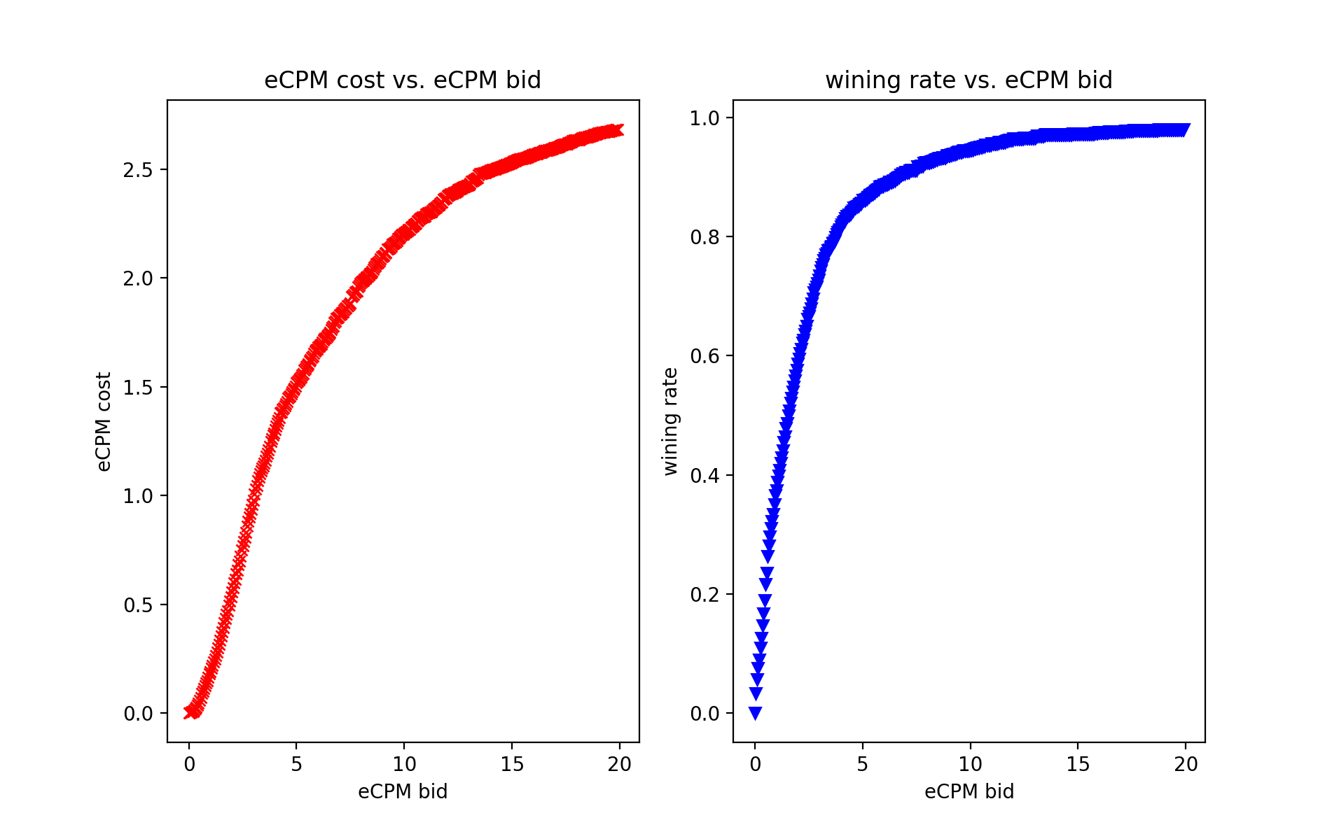
Figure 1: (left) eCPM cost c.d.f vs. eCPM bid; (right) win rate c.d.f vs. eCPM bid.

To cluster advertisers into different segmentations, we have three views of information: (i) advertisers’ textual descriptions; (ii) advertisers’ win-rate cumulative distribution function (i.e., c.d.f for short); (iii) advertisers’ eCPM cost c.d.f. In advertising, win rate is a percentage metric in programmatic media marketing that measures the number of impressions won over the number of impressions bid, and win rate cumulative distribution function (c.d.f) measures the percentages of impressions won blow certain bids. eCPM cost is the effective cost per thousand impressions given the bid, and eCPM cost cumulative distribution function (c.d.f) measures the cost of impressions below certain bids. Fig.1 give an example of advertisers’ win-rate c.d.f and eCPM cost c.d.f (a.k.a bid landscape model that allows one to estimate performance of advertising campaigns under different bidding scenarios). We extract advertisers’ textual description for clustering purpose.

Connection to the proposed robust clustering method Our method consists of two key steps: (i) generating clustering results using each view information and obtain the co-association matrix of $\tilde{M}$ of Eq.(10) (ii) using the robust consensus clustering model of Eq.(Relaxation in continuous domain) to generate the consensus clustering results.

Similarity Computation using KS Statistics Given the pairwise similarity in each view, a natural way is to segment different them into different disjoint $K$ subsets where each subset denotes a clustering using graph cut type algorithm (e.g., Normalized Cut). In order to generate the clustering results using win-rate c.d.f and eCPM cost c.d.f, we refer to Kolmogorov- Smirnov (KS for short) statistics (?), (?), which offers a nonparametric way to quantify the distances between the empirical distribution functions. The traditional way is to compare the mean or median of two distributions with parametric tests (using Z-test or t-test), or non-parametric tests (Mann-Whitney or Kruskal-Wallis test). However, these methods only consider the domain differences of two distributions, not the scale. Moreover, some parametric methods impose strong normal distribution assumption, which is not realistic for ad campaigns.

Suppose we have independent identical distributed (i.i.d) samples $X_{1},\cdots,X_{m}$ of size $m$ with cumulative distribution function (c.d.f) $F(x)$ and the second i.i.d sample $Y_{1},...,Y_{n}$ of size $n$ with c.d.f $G(x)$. One wants to test the null hypothesis ($H_{0}:F=G$) vs. the alternative ($H_{1}:F\neq G$). $F_{m}(x)$ and $G_{n}(x)$ are the corresponding c.d.fs, where

$$F_{m}(x)=\frac{1}{m}\sum_{i=1}^{m}I(X_{i}\leq x),\;\;\;G_{n}(x)=\frac{1}{n}\sum_{i=1}^{n}I(Y_{i}\leq x).$$

The KS test statistic is defined as the maximum value of the absolute difference between two c.d.f.s, i.e.,

$$D_{mn}=\sqrt{\frac{mn}{m+n}}\sup_{x}|F_{m}(x)-G_{n}(x)|$$ (39)

The distribution of KS test statistic doesn’t depend on the known distribution. In addition, it converge to KS distribution, i.e.

$$\lim_{m,n\rightarrow\infty}P(D_{mn}\leq z)=1-2\sum_{i=1}^{\infty}(-1)^{i-1}exp(-2i^{2}z^{2})$$ (40)

This nice property enables the wide application of KS-statistics for solving real-world problems. In the context of advertiser clustering, let $f_{m}(i)$ be the winning rate function c.d.f for advertiser $i$ generated from $m$ observations, and $f_{n}(j)$ be the win rate function c.d.f for advertiser $j$ generated from $n$ observations, then distance $dist(i,j)$ between $i$ and $j$ is defined as:

$$dist(i,j|m,n)=\sqrt{\frac{mn}{m+n}}\sup_{x}|f_{m}(BF_{i})-f_{n}(BF_{j})|.$$ (41)

Therefore the similarity (denoted as $S^{\text{win}}_{ij}$) of pairwise advertisers $i,j$ is computed based on

$$S^{\text{win}}_{ij}=\left\{\begin{matrix}1;\;\;\;\text{if}\;\;\;dist(i,j|m,n)\leq C_{\alpha}\\ 0;\;\;\;\;\;\;\;\;\;\;\;\;\;\;\;\;\;\text{otherwise},\end{matrix}\right.$$ (42)

where $C_{\alpha}$ is the confidence value set corresponding to $p$-value. In particular, if one chooses a critical value $C_{\alpha}$ such that

$$\Pr(dist(i,j|m,n)>C_{\alpha})=\alpha,$$

then a band of width $C_{\alpha}$ around the distribution of $dist(i,j|m,n)$ will entirely contain the estimated value with probability $(1-\alpha)$. eCPM cost similarity is computed using the same way.

Experimental Results

The ad campaign data are collected from a major web portal. In this study, we consider 1,268 advertisers over a week. As is introduced in Kolmogorov-Smirnov statistics, we set $p$-value = $\{0.01,0.05,0.1\}$ ($p=0.01$ lower bound and $p=0.1$ upper bound). Table 4 shows the clustering number using the win rate c.d.f and eCPM cost c.d.f features respectively. Clearly, when $p$-value increases, the critical $C_{\alpha}$-value for determination of similar campaigns decreases because there are smaller chances for advertisers falling in the range of $P(dist(i,j|m,n))>C_{\alpha}$ using Eq.(42).

Table 4: # of clusterings at different $p$

Category	$p=0.01$	$p=0.05$	$p=0.1$
win rate	65	47	32
eCPM	73	51	40

Consistency of clustering For any pairwise advertisers, if both win rate c.d.f and eCPM cost c.d.f cluster them to the same group (or the different group), then they are viewed as true consistency, otherwise, if one method clusters them in the same group while the other clusters them in different groups, then viewed as inconsistency (FPN). More mathematically, let $C_{i},C_{j}$ be the cluster label obtained using eCPM cost for $i,j$ and let $\ell_{i},\ell_{j}$ be the cluster using win rate for $i$ and $j$ , then

$${TPN}=\sum_{i<j}\Big{[}\Big{(}I_{C_{i}=C_{j}}\Big{)}\bigcap\Big{(}I_{\ell_{i}=\ell_{j}}\Big{)}\Big{]}\bigcup\Big{[}\Big{(}I_{C_{i}\neq C_{j}}\Big{)}\bigcap\Big{(}I_{\ell_{i}\neq\ell_{j}}\Big{)}\Big{]}$$

$${FPN}=\sum_{i<j}\Big{[}\Big{(}I_{C_{i}=C_{j}}\Big{)}\bigcap\Big{(}I_{\ell_{i}\neq\ell_{j}}\Big{)}\Big{]}\bigcup\Big{[}\Big{(}I_{C_{i}\neq C_{j}}\Big{)}\bigcap\Big{(}I_{\ell_{i}=\ell_{j}}\Big{)}\Big{]}$$

Table 5: Consistency of clustering using win rate c.d.f and eCPM cost c.d.f

Category	Percentage %
TPN	74.21%
FPN	25.79%

Table 5 shows the consensus clustering results using these two views of features. Clearly, around three fourth advertisers share very similar results even using different features.

Table 6: Forecast impression error (the smaller, the better)

Feature type	# forecasting error
win c.d.f	18.10%
eCPM c.d.f	20.31%
textual	30.98%
consensus clustering	17.87%
propose method	15.96%

Table 7: Forecast spend error (the smaller, the better)

Feature type	# forecasting error
win c.d.f	12.34%
eCPM c.d.f	13.56%
textual	25.78%
consensus clustering	12.78%
propose method	9.64%

Clustering performance Given the fact that we do not have ground-truth for advertiser clustering results, we cannot directly evaluate the performance of our method. Instead, we view the robust consensus clustering result as the advertiser segmentation result, and use it to re-generate the eCPM cost and win-rate c.d.ds using all the information from the same advertiser clusters. With the updated eCPM cost (?) and win-rate c.d.f.s, we forecast the clicks and spend, and compute the relative percentage errors to validate the performance of updated eCPM cost and win-rate distributions. In particular, if the clustering result is better, then the re-generated eCPM and win-rate distributions are more accurate.

$$\texttt{ \text{\# Impression} = \text{Total supply}}\times\texttt{\text{win-rate} }$$

$$\texttt{\text{\# Spend } = \text{\# Impression}}\times\texttt{ \text{ eCPM cost}}$$

which is to say, the forecasted impression (# Impression) is equal to the total number of supplies by applying the win-rate, and the forecasted spend is equal to the forecasted impressions multiplied by eCPM cost for per impression. The accurate estimation of win-rate and eCPM will make the forecasted impressions and spend more accurate.

Therefore, we re-generate the eCPM and win-rate distributions using the following several consensus clustering results: (i) only ads textual; (ii) only win-rate; (iii) only eCPM cost; (iv) proposed robust consensus clustering; (v) consensus clustering using $\ell_{2}$ distance; and compare their performances. The mean of absolute percentage error is defined as: $MAPE=\frac{1}{n}\sum_{i=1}^{n}\frac{|y_{i}-\hat{y}_{i}|}{y_{i}},$ where $y_{i}$ is the ground-truth for advertiser $i$ and $\hat{y}_{i}$ is the forecasted impression (or spend) for advertiser $i$. The smaller of these values, the better performance of clustering. Tables 6,  7 show the forecasted impression and spend errors, respectively. Thanks to the proposed robust consensus clustering algorithm, the forecasting error has been dropped significantly for both forecasted clicks and spend.

Conclusion

This paper presents a novel approach for consensus clustering. The new clustering objective is more robust to noise and outliers. We formulate the problem rigorously and show that the optimal solution can be derived using ADMM algorithm. We apply our method to solve real-world advertiser segmentation problem, where the consensus clustering produces better forecasting results.

References

- [Azimi and Fern 2009] Azimi, J., and Fern, X. 2009. Adaptive cluster ensemble selection. In IJCAI, 992–997.
- [Bertsekas 1996] Bertsekas, D. 1996. Constrained Optimization and Lagrange Multiplier Methods. Athena Scientific.
- [Cai, Nie, and Huang 2013] Cai, X.; Nie, F.; and Huang, H. 2013. Multi-view k-means clustering on big data. In IJCAI, 2598–2604.
- [Cui et al. 2011] Cui, Y.; Zhang, R.; Li, W.; and Mao, J. 2011. Bid landscape forecasting in online ad exchange marketplace. In Proceedings of the 17th ACM SIGKDD International Conference on Knowledge Discovery and Data Mining, KDD ’11, 265–273.
- [Dalal and Triggs 2005] Dalal, N., and Triggs, B. 2005. Histograms of oriented gradients for human detection. In CVPR, 886–893 vol. 1.
- [Domeniconi and Al-Razgan 2009] Domeniconi, C., and Al-Razgan, M. 2009. Weighted cluster ensembles: Methods and analysis. ACM Trans. Knowl. Discov. Data 2(4):17:1–17:40.
- [Dudoit and Fridlyand 2003] Dudoit, S., and Fridlyand, J. 2003. Bagging to improve the accuracy of a clustering procedure. Bioinformatics 19(9):1090–1099.
- [Dueck and Frey 2007] Dueck, D., and Frey, B. J. 2007. Non-metric affinity propagation for unsupervised image categorization. In ICCV, 1–8.
- [Fei-Fei, Fergus, and Perona 2007] Fei-Fei, L.; Fergus, R.; and Perona, P. 2007. Learning generative visual models from few training examples: An incremental bayesian approach tested on 101 object categories. Comput. Vis. Image Underst. 106(1):59–70.
- [Fern and Brodley 2004] Fern, X. Z., and Brodley, C. E. 2004. Solving cluster ensemble problems by bipartite graph partitioning. In Proceedings of the Twenty-first International Conference on Machine Learning, ICML ’04. New York, NY, USA: ACM.
- [Filkov and Skiena 2004] Filkov, V., and Skiena, S. 2004. Integrating microarray data by consensus clustering. International Journal on Artificial Intelligence Tools 13(4):863–880.
- [Gao 2016] Gao, Junning; Yamada, M. K. S. M. H. Z. S. 2016. A robust convex formulation for ensemble clustering. IJCAI, 1476–1482.
- [Gates, Haidar, and Dongarra 2014] Gates, M.; Haidar, A.; and Dongarra, J. 2014. Accelerating eigenvector computation in the nonsymmetric eigenvalue problem. In VECPAR 2014.
- [Girshick et al. 2013] Girshick, R. B.; Donahue, J.; Darrell, T.; and Malik, J. 2013. Rich feature hierarchies for accurate object detection and semantic segmentation. CoRR abs/1311.2524.
- [Huang, Lai, and Wang 2016] Huang, D.; Lai, J.; and Wang, C. 2016. Robust ensemble clustering using probability trajectories. IEEE Transactions on Knowledge & Data Engineering 28(5):1312–1326.
- [Jain, Murty, and Flynn 1999] Jain, A. K.; Murty, M. N.; and Flynn, P. J. 1999. Data clustering: A review. ACM Comput. Surv. 31(3):264–323.
- [Kolmogorov 1933] Kolmogorov, A. N. 1933. Sulla determinazione empirica di una legge di distribuzione. Giornale dell’Istituto Italiano degli Attuari 4(1):83–91.
- [Li and Ding 2008] Li, T., and Ding, C. H. Q. 2008. Weighted consensus clustering. In Proceedings of the SIAM International Conference on Data Mining, SDM 2008, April 24-26, 2008, Atlanta, Georgia, USA, 798–809.
- [Li, Ding, and Jordan 2007] Li, T.; Ding, C.; and Jordan, M. I. 2007. Solving consensus and semi-supervised clustering problems using nonnegative matrix factorization. In Proceedings of the 2007 Seventh IEEE International Conference on Data Mining, ICDM ’07, 577–582.
- [Liu, Latecki, and Yan 2010] Liu, H.; Latecki, L. J.; and Yan, S. 2010. Robust clustering as ensembles of affinity relations. In NIPS, 1414–1422.
- [Mahdian and Wang 2009] Mahdian, M., and Wang, G. 2009. Clustering-based bidding languages for sponsored search. In Algorithms - ESA 2009, 17th Annual European Symposium, Copenhagen, Denmark, September 7-9, 2009. Proceedings, 167–178.
- [OJA 1996] 1996. A comparative study of texture measures with classification based on featured distributions. Pattern Recognition 29(1):51 – 59.
- [Oliva and Torralba 2001] Oliva, A., and Torralba, A. 2001. Modeling the shape of the scene: A holistic representation of the spatial envelope. Int. J. Comput. Vision 42(3):145–175.
- [Roth et al. 2003] Roth, V.; Laub, J.; Kawanabe, M.; and Buhmann, J. M. 2003. Optimal cluster preserving embedding of nonmetric proximity data. IEEE Trans. Pattern Anal. Mach. Intell. 25(12):1540–1551.
- [Shi and Malik 2000] Shi, J., and Malik, J. 2000. Normalized cuts and image segmentation. IEEE Trans. Pattern Anal. Mach. Intell. 22(8):888–905.
- [Smirnov 1948] Smirnov, N. 1948. Table for estimating the goodness of fit of empirical distributions. The Annals of Mathematical Statistics 19(2):279–281.
- [Strehl and Ghosh 2003] Strehl, A., and Ghosh, J. 2003. Cluster ensembles — a knowledge reuse framework for combining multiple partitions. J. Mach. Learn. Res. 3:583–617.
- [Talwalkar et al. 2013] Talwalkar, A.; Mackey, L. W.; Mu, Y.; Chang, S.; and Jordan, M. I. 2013. Distributed low-rank subspace segmentation. In ICCV, 3543–3550.
- [Tao et al. 2017] Tao, Z.; Liu, H.; Li, S.; Ding, Z.; and Fu, Y. 2017. From ensemble clustering to multi-view clustering. In IJCAI-17, 2843–2849.
- [Topchy, Jain, and Punch 2004] Topchy, A. P.; Jain, A. K.; and Punch, W. F. 2004. A mixture model for clustering ensembles. In SDM, 379–390.
- [Torresani, Szummer, and Fitzgibbon 2010] Torresani, L.; Szummer, M.; and Fitzgibbon, A. 2010. Efficient object category recognition using classemes. In ECCV, 776–789.
- [Wang et al. 2014] Wang, Y.; Lin, X.; Wu, L.; Zhang, W.; and Zhang, Q. 2014. Exploiting correlation consensus: Towards subspace clustering for multi-modal data. In ACM MM’14, 981–984. ACM.
- [Wang, She, and Cao 2013] Wang, C.; She, Z.; and Cao, L. 2013. Coupled clustering ensemble: Incorporating coupling relationships both between base clusterings and objects. In ICDE, Brisbane, Australia, 374–385.
- [Winn and Jojic 2005] Winn, J., and Jojic, N. 2005. Locus: learning object classes with unsupervised segmentation. In ICCV, 756–763 Vol. 1.
- [Wright et al. 2009] Wright, J.; Yang, A. Y.; Ganesh, A.; Sastry, S. S.; and Ma, Y. 2009. Robust face recognition via sparse representation. IEEE Trans. Pattern Anal. Mach. Intell. 31(2):210–227.
- [Xu and Wunsch 2005] Xu, R., and Wunsch, II, D. 2005. Survey of clustering algorithms. Trans. Neur. Netw. 16(3):645–678.
- [Zhou et al. 2015] Zhou, P.; Du, L.; Wang, H.; Shi, L.; and Shen, Y.-D. 2015. Learning a robust consensus matrix for clustering ensemble via kullback-leibler divergence minimization. In IJCAI, 4112–4118.