RIS-Assisted Receive Quadrature Spatial Modulation with Low-Complexity
Greedy Detection

Abstract

In this paper, we propose a novel reconfigurable intelligent surface (RIS)-assisted wireless communication scheme which uses the concept of spatial modulation, namely RIS-assisted receive quadrature spatial modulation (RIS-RQSM). In the proposed RIS-RQSM system, the information bits are conveyed via both the indices of the two selected receive antennas and the conventional in-phase/quadrature (IQ) modulation. We propose a novel methodology to adjust the phase shifts of the RIS elements in order to maximize the signal-to-noise ratio (SNR) and at the same time to construct two separate PAM symbols at the selected receive antennas, as the in-phase and quadrature components of the desired IQ symbol. An energy-based greedy detector (GD) is implemented at the receiver to efficiently detect the received signal with minimal channel state information (CSI) via the use of an appropriately designed one-tap pre-equalizer. We also derive a closed-form upper bound on the average bit error probability (ABEP) of the proposed RIS-RQSM system. Then, we formulate an optimization problem to minimize the ABEP in order to improve the performance of the system, which allows the GD to act as a near-optimal receiver. Extensive numerical results are provided to demonstrate the error rate performance of the system and to compare with that of a prominent benchmark scheme. The results verify the remarkable superiority of the proposed RIS-RQSM system over the benchmark scheme.

I Introduction

In the past few years, various wireless communication technologies have emerged with an aim to support high demands for connectivity and an immense increase in mobile data traffic. Among these, reconfigurable intelligent surfaces (RISs), also known as intelligent reflecting surfaces (IRSs), represents a key innovation that has drawn significant attention from researchers in both academia and industry [1] and is foreseen to be a potential candidate for 6th generation (6G) networks [2, 3]. An RIS is a surface of electromagnetic meta-material consisting of a large number of small, low-cost and energy-efficient reflecting elements that are able to control the scattering and propagation in the channel by inducing a pre-designed phase shift to the impinging wave. From this perspective, RIS technology represents a revolutionary paradigm that can transform the uncontrollable disruptive propagation environment into a smart radio environment [2, 4], thus enhancing the received signal quality [5, 6].

On the other hand, spatial modulation (SM) [7, 8] and its variants such as generalized spatial modulation (GSM) [9], receive spatial modulation (RSM) [10, 11], and quadrature spatial modulation (QSM) [12], have been widely investigated in the last two decades as a promising technology for beyond-5th-generation (B5G) networks. SM uses the indices of the transmit/receive antennas to convey the information bits. It exploits the channel attributes to simplify the transceiver structure in order to provide a more energy-efficient solution compared with other conventional multiple-input multiple-output (MIMO) techniques [13].

The implicit advantages of both RIS and SM technology have motivated researchers to combine these two advanced technologies to obtain a reliable energy-efficient approach in order to achieve so-called green or sustainable wireless communications. Specifically, in [14], two fundamental RIS-based index modulation (IM) techniques were proposed, i.e., RIS-space-shift keying (RIS-SSK) and RIS-spatial modulation (RIS-SM). In both scenarios, the RIS-access point (RIS-AP) approach was implemented, in which the RIS forms part of the transmitter, and the index of the receive antennas is used to convey the data bits. The numerical results confirm a significant superiority of these RIS-aided schemes compared to conventional MIMO schemes. Various principles of RIS-based SM (also known as metasurface-based modulation) were introduced in [15]. The authors of [16] proposed an RIS-SSK system with multiple transmit antennas in which the information bits map to the transmit antenna index and the single-antenna receiver receives the signal reflected from the RIS. Various scenarios with ideal and non-ideal transceivers were investigated and the error rate performance of each scenario was analyzed. The results indicate that maximizing the signal-to-noise ratio (SNR) at the receiver is not a good approach for the transmit RIS-SSK setting, and in fact shows a relatively poor performance. In light of this, in [17] the authors proposed an optimization algorithm for the transmit RIS-SSK system to maximize the minimum Euclidean distance among the received symbols. Using this approach, a performance improvement is achieved at the expense of an increased computational complexity. Moreover, in [18], adopting a similar approach, the authors proposed a joint optimization of the power allocation matrix and the phase shifts of the RIS elements. An RIS-based SM system with both the transmit and receive antenna index modulation was proposed in [19] to increase the spectral efficiency. However, the results show that the error rate performance of the transmit SM bits is extensively lower than that of the receive SM bits; this is due to a reduction in the resulting channel-imprinted Euclidean distances. RIS-aided receive quadrature reflecting modulation (RIS-RQRM) proposed in [20] is another interesting approach in which QSM is applied within the receive antenna array. In this scenario, the RIS is divided into two halves, and each half targets the real or imaginary part of the signal at the two selected receive antennas in order to double the throughput; however, the SNR at the receiver is significantly reduced due the reduction in the number of RIS elements per targeted antenna. Inspired by RIS-RQRM and [19], an IRS-assisted transceiver QSM (IRS-TQSM) scheme was proposed in [21] which applies QSM at both the transmitter and the receiver. In [22, 23], generalized SSK (GSSK) and GSM approaches have been implemented in an RIS-assisted wireless system. In both scenarios, the RIS is divided into multiple parts to target multiple antennas at the receiver; hence, the throughput can be increased at the expense of a decrease in the SNR at the target antennas. The concept of SM has also been applied within the RIS entity in [24, 25, 26] in order to transmit additional data bits. This is an exciting approach to transmit the environmental data collected by the RIS; however, experimental results show a very large degradation in the error rate performance of the SM symbol, that is due to the similarity within the possible (noise-free) received signals. In order to tackle the problem of the SNR decrease due to grouping of the RIS elements, in [27] we proposed a new paradigm, namely RIS-assisted receive quadrature space-shift keying (RIS-RQSSK) in order to simultaneously target two receive antennas. An optimization problem was defined to maximize the SNR of the real part of the signal at one antenna and, at the same time, of the imaginary part of the signal at the second antenna. The spectral efficiency of this approach is increased without any degradation in the SNR. However, the throughput of the RIS-RQSSK system is limited and can only be increased by increasing the number of receive antennas which is not a viable option in practice.

Against this background, in this paper we introduce a new RIS-assisted quadrature scheme in which, in addition to mapping the information bits independently to two indices of receive antennas, additional bits are transmitted via conventional in-phase/quadrature (IQ) modulation. The contributions of this paper are as follows:

• To improve the spectral efficiency of RIS-RQSSK while preserving its excellent performance, we propose an RIS-assisted receive quadrature spatial modulation (RIS-RQSM) system. In particular, all RIS elements target two independently selected receive antennas to convey the information bits. In this scenario, we introduce a novel idea to optimize the phase shifts of the RIS elements in order to not only maximize the SNR components associated to the real and imaginary parts of the signal at the receive antennas, but also to help in constructing the in-phase (I) and quadrature (Q) components of the symbol at the two separate antennas. Specifically, the phase of the desired IQ symbol is created by adjusting the phase shift of the RIS elements, while a positive symbol selected from a specific pre-designed PAM constellation forms the amplitude of that IQ symbol. That is, in the proposed RIS-RQSM system, in contrast to conventional IQ modulation, the transmitter constructs the IQ symbol at the receiver with the aid of the RIS elements and a single radio frequency (RF) chain.

• We propose an energy-based greedy detector (GD) at the receiver to detect the indices of the selected antennas with low complexity. Then, the I and Q symbols can be detected independently by using a one-dimensional maximum likelihood (ML) detector at each of the detected antennas. We also propose and design a one-tap zero-forcing (ZF) pre-equalizer which remarkably reduces the channel state information (CSI) requirement at the receiver. This yields a significant reduction in the feedback payload.

• We analyze the average bit error probability (ABEP) of the proposed RIS-RQSM system with the GD receiver and derive a closed-form upper bound which is tight, especially at high SNR values. Then, we propose an optimization problem to design an IQ modulation scheme in order to minimize the ABEP. We utilize some accurate approximations to reduce the complexity of the optimization problem and derive an analytical solution. Indeed, optimizing the IQ modulation enables the system to use the GD as an alternative to the ML detector. The results show that the GD in the RIS-RQSM system with optimized constellation performs considerably close to the ML detector, such that the performance gap is negligible.

• Finally, we compare the bit error rate (BER) performance results with those of the most prominent benchmark scheme. The results show that the proposed RIS-RQSM system substantially outperforms the benchmark scheme. This performance improvement improves with an increasing number of receive antennas.

The rest of this paper is organized as follows. The RIS-RQSM system model is described in Section II. In Section III, we summarize the transceiver design of the RIS-RQSSK system of [27], which forms the baseline model for the proposed system. The transmitter and receiver structure design for the proposed RIS-RQSM system is presented in detail in Section IV. The ABEP performance of the proposed RIS-RQSM system is analyzed in Section V. In Section VI, we formulate the optimization problem to minimize the system error rate performance and determine its analytical solution. In Section VII, we provide numerical results and comparisons with the benchmark scheme. Finally, Section VIII concludes this paper.

Notation: Boldface lower-case letters denote column vectors, and boldface upper-case letters denote matrices. $\left(\cdot\right)^{\mathcal{R}}$ and $\left(\cdot\right)^{\mathcal{I}}$ denote the real and imaginary components of a scalar/vector, respectively. $\left(\cdot\right)^{\star}$ represents the optimum value of a scalar/vector variable. $\mathsf{\mathbb{E}}\left\{\cdot\right\}$ and $\mathbb{V}\left\{\cdot\right\}$, respectively, denote the expectation and variance operator. $\mathcal{N}\left(\mu,\sigma^{2}\right)$ (resp., $\mathcal{CN}\left(\mu,\sigma^{2}\right)$) represents the normal (resp., complex normal) distribution with mean $\mu$ and variance $\sigma^{2}$. For a real/complex scalar $s$, $\left|s\right|$ denotes the absolute value, while for a set $\mathcal{S}$, $\left|\mathcal{S}\right|$ denotes its cardinality. $\text{sgn}\left(\cdot\right)$ represents the sign function which determines the sign of a real variable, i.e., for $x\neq 0$, it is defined as $\text{sgn}\left(x\right)=\left\{+1\text{ if }x>0,\,-1\text{ if }x<0\right\}$. Finally, the set of complex matrices of size $m\times n$ is denoted by $\mathbb{C}^{m\times n}$.

II System Model

In this section, we describe the system model for the proposed RIS-assisted receive quadrature spatial modulation (RIS-RQSM) scheme. A schematic of the RIS-RQSM system is presented in Fig. 1. We consider the RIS-AP model [5, 6], where the RIS forms part of the transmitter and reflects the incident wave emitted from a single transmit antenna which is located in the vicinity of the RIS such that the path loss and scattering of the link between the RIS and the transmit antenna is negligible. The RIS is comprised of $N$ reflecting elements whose vector of phase shifts $\boldsymbol{\theta}\in\mathbb{C}^{N\times 1}$ is controlled by the transmitter to convey information. Here we assume lossless reflection from the RIS, i.e., $\left|\theta_{i}\right|=1$ for $i=1,2,\dots,N$. The receiver is equipped with $N_{r}$ antennas and is placed far from the transmitter. We assume that the receiver can only receive the signal reflected from the RIS elements through the wireless fading channel $\mathbf{H}\in\mathbb{C}^{N_{r}\times N}$, whose elements are assumed to be independent and identically distributed (i.i.d.) according to $\mathcal{CN}\left(0,1\right)$. In this scenario, the input data stream is split into packets of $\log_{2}MN_{r}^{2}$ bits. The first $\log_{2}N_{r}^{2}$ bits are used to independently select two receive antennas to convey the spatial symbol, and the remaining $\log_{2}M$ bits determine the desired IQ symbol that is selected from an $M$-ary QAM constellation. Unlike in conventional communication systems, in the RIS-RQSM system the selected IQ symbol is not transmitted through a single-antenna transmitter, but is created at the selected receive antennas via both adjusting the RIS phase shifts and emitting a specific PAM symbol from the transmit antenna, with a property that the I component appears on the first selected antenna, while the Q component appears on the second selected antenna. Thus, the RIS-RQSM scheme represents a significant generalization of the RIS-assisted receive quadrature space-shift keying (RIS-RQSSK) system described in [27]. In RIS-RQSSK, an RF source is used to transmit a constant signal toward the RIS; therefore, only a spatial symbol can be transmitted, while the PAM signal in RIS-RQSM enables the transmitter to transfer additional data bits via IQ modulation. In the next section, we will provide a brief overview of the RIS-RQSSK system. Then, the proposed RIS-RQSM system will be described in Section IV.

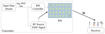
Figure 1: A schematic representation of RIS-assisted receive quadrature spatial modulation (RIS-RQSM) system (in RIS-RQSSK system, an RF source with constant energy is used).

III RIS-Assisted Receive Quadrature Space-Shift Keying [27]

In this section, we summarize the system model of the RIS-RQSSK scheme of [27] and outline its phase shift optimization procedure. In the RIS-RQSSK system, the transmitter is equipped with an RF source with constant energy $E_{s}$. In this scenario, two receive antennas are independently selected according to two packets of $\log_{2}N_{r}$ input data bits. Then, the transmitter reflects the signal to the receiver through the RIS, aiming to simultaneously maximize the SNR associated to the real part of the signal at the first selected receive antenna $m$, while also maximizing the signal-to-noise ratio (SNR) associated to the imaginary part of the signal at the second selected receive antenna $n$. For this system, the real and imaginary components of the baseband received signal at the selected antennas $m$ and $n$, respectively, are given by

$$y_{m}^{\mathcal{R}} =\sqrt{E_{s}}\left[\mathbf{h}_{m}^{\mathcal{R}}\boldsymbol{\theta}^{\mathcal{R}}-\mathbf{h}_{m}^{\mathcal{I}}\boldsymbol{\theta}^{\mathcal{I}}\right]+n_{m}^{\mathcal{R}},$$ (1)

$$y_{n}^{\mathcal{I}} =\sqrt{E_{s}}\left[\mathbf{h}_{n}^{\mathcal{R}}\boldsymbol{\theta}^{\mathcal{I}}+\mathbf{h}_{n}^{\mathcal{I}}\boldsymbol{\theta}^{\mathcal{R}}\right]+n_{n}^{\mathcal{I}},$$ (2)

where $\mathbf{h}_{l}=\left[h_{l,1},h_{l,2},\dots,h_{l,N}\right]$ is the $l$-th row of $\mathbf{H}$, and $n_{l}\in\mathbb{C}$ is the additive white Gaussian noise at the $l$-th receive antenna that is distributed according to $\mathcal{CN}\left(0,N_{0}\right)$. To maximize both SNR components associated to the real and imaginary parts of the selected receive antennas $m$ and $n$, a max-min optimization problem was defined as

$$\underset{\boldsymbol{\theta}^{\mathcal{R}},\boldsymbol{\theta}^{\mathcal{I}}}{\max} \ \min\left(\left|\mathbf{h}_{m}^{\mathcal{R}}\boldsymbol{\theta}^{\mathcal{R}}-\mathbf{h}_{m}^{\mathcal{I}}\boldsymbol{\theta}^{\mathcal{I}}\right|,\left|\mathbf{h}_{n}^{\mathcal{R}}\boldsymbol{\theta}^{\mathcal{I}}+\mathbf{h}_{n}^{\mathcal{I}}\boldsymbol{\theta}^{\mathcal{R}}\right|\right)$$ (3)

s.t. $$\ \left(\theta_{i}^{\mathcal{R}}\right)^{2}+\left(\theta_{i}^{\mathcal{I}}\right)^{2}=1,\ \mbox{for all}\;i=1,2,\dots,N.$$

Taking the case where the noise-free signal components in (1) and (2) are positive, the optimal values of $\left\{\theta_{i}^{\mathcal{R}}\right\}$ and $\left\{\theta_{i}^{\mathcal{I}}\right\}$ are given by

$$\theta_{i}^{\mathcal{R}\star}=\frac{\lambda A_{i}+\left(1-\lambda\right)B_{i}}{\sqrt{\left(\lambda A_{i}+\left(1-\lambda\right)B_{i}\right)^{2}+\left(\lambda C_{i}+\left(1-\lambda\right)D_{i}\right)^{2}}},$$ (4)

for all $i=1,2,\dots,N$, and

$$\theta_{i}^{\mathcal{I}\star}=\frac{\lambda C_{i}+\left(1-\lambda\right)D_{i}}{\sqrt{\left(\lambda A_{i}+\left(1-\lambda\right)B_{i}\right)^{2}+\left(\lambda C_{i}+\left(1-\lambda\right)D_{i}\right)^{2}}},$$ (5)

for all $i=1,2,\dots,N$, where we define

$$A_{i}=h_{m,i}^{\mathcal{R}},\ B_{i}=h_{n,i}^{\mathcal{I}},\ C_{i}=-h_{m,i}^{\mathcal{I}},\ \text{and}\ D_{i}=h_{n,i}^{\mathcal{R}},$$ (6)

to simplify the notation, and where, for $N\gg 1$, the value of $\lambda\in(0,1)$ is the solution to

$$f(\lambda)\triangleq\sum_{i=1}^{N}\frac{\left(A_{i}-B_{i}\right)\left(\lambda A_{i}+\left(1-\lambda\right)B_{i}\right)+\left(C_{i}-D_{i}\right)\left(\lambda C_{i}+\left(1-\lambda\right)D_{i}\right)}{\sqrt{\left(\lambda A_{i}+\left(1-\lambda\right)B_{i}\right)^{2}+\left(\lambda C_{i}+\left(1-\lambda\right)D_{i}\right)^{2}}}=0.$$ (7)

In addition, with the optimal phase shift values given in (4) and (5), the resulting SNR components have the same value, i.e., we have

$$\mathbf{h}_{m}^{\mathcal{R}}\boldsymbol{\theta}^{\mathcal{R}\star}-\mathbf{h}_{m}^{\mathcal{I}}\boldsymbol{\theta}^{\mathcal{I}\star}=\mathbf{h}_{n}^{\mathcal{R}}\boldsymbol{\theta}^{\mathcal{I}\star}+\mathbf{h}_{n}^{\mathcal{I}}\boldsymbol{\theta}^{\mathcal{R}\star}.$$

Finally, at the receiver, a simple but effective greedy detector (GD) is employed to detect the selected receive antennas without the need for any knowledge of the CSI at the receiver. The GD operates via

$$\hat{m} =\arg\max_{m\in\{1,2,\dots,N_{r}\}}\left\{\left(y_{m}^{\mathcal{R}}\right)^{2}\right\},$$ (8)

$$\hat{n} =\arg\max_{n\in\{1,2,\dots,N_{r}\}}\left\{\left(y_{n}^{\mathcal{I}}\right)^{2}\right\}.$$ (9)

The performance results have demonstrated the superiority of the RIS-RQSSK system over comparable benchmark schemes. This motivates us to extend this scheme to the context of QSM, which is the subject of the next section.

IV RIS-Assisted Receive Quadrature Spatial Modulation

In general, while the spectral efficiency of an SSK system can be increased by extending it to the corresponding quadrature SSK system, it can be further improved by implementing a conventional IQ modulation on top of the antenna index modulation. In the conventional receive quadrature SM (RQSM), the transmit vector can be designed to place the real and imaginary parts of the symbol separately at a specific position of the real and imaginary receive vector. On the other hand, in the RIS-RQSM scheme, the transmitter is equipped with only one antenna and therefore can only transmit one symbol in each symbol interval. In addition, since the real and imaginary parts of the desired symbol needs to be separated at the receiver, the transmitter can only perform amplitude modulation through the RF source to be detectable at the receiver (as also suggested in [20] for the RIS-RQRM scheme), i.e., it is not feasible to transmit a QAM symbol and receive the I and Q components separately at two different receive antennas. To tackle this problem, in the proposed RIS-RQSM system we introduce a new paradigm in order to construct an $M$-ary QAM symbol (in fact, two independent symbols from identical $\sqrt{M}$-ary PAM constellations) at the receiver via the adjustment of both the amplitude of the RF source and the phase shifts of the RIS elements. Therefore, in the RIS-RQSM system the rate is $R=\log_{2}M+2\log_{2}N_{r}$ bits per channel use (bpcu). In this scenario, the desired received signal components are given by

$$y_{m}^{\mathcal{R}} =\left[\mathbf{h}_{m}^{\mathcal{R}}\boldsymbol{\theta}^{\mathcal{R}}-\mathbf{h}_{m}^{\mathcal{I}}\boldsymbol{\theta}^{\mathcal{I}}\right]Gs+n_{m}^{\mathcal{R}},$$ (10)

$$y_{n}^{\mathcal{I}} =\left[\mathbf{h}_{n}^{\mathcal{R}}\boldsymbol{\theta}^{\mathcal{I}}+\mathbf{h}_{n}^{\mathcal{I}}\boldsymbol{\theta}^{\mathcal{R}}\right]Gs+n_{n}^{\mathcal{I}},$$ (11)

where $s$ is the transmit symbol selected from a specific positive real PAM constellation, denoted by $\mathcal{P}_{\mathrm{RF}}$. The amplitudes in $\mathcal{P}_{\mathrm{RF}}$ are the magnitudes of the complex symbols in an $M$-ary QAM constellation $\mathcal{M}$ with average energy $E_{s}$, i.e., $s=\left|x\right|$ where $x\in\mathcal{M}$ is the desired IQ symbol, and $G>0$ is a one-tap zero-forcing (ZF) pre-equalizer to be defined later.

To produce the desired $M$-ary QAM signal at the receiver, we modify the problem in (3) to accommodate both the index modulation and IQ modulation as

$$\underset{\boldsymbol{\theta}^{\mathcal{R}},\boldsymbol{\theta}^{\mathcal{I}}}{\max} \ \min\left(Y_{R},\delta Y_{I}\right)$$ (12a)

s.t. $$\;Y_{R}=\text{sgn}\left(x^{\mathcal{R}}\right)\left(\mathbf{h}_{m}^{\mathcal{R}}\boldsymbol{\theta}^{\mathcal{R}}-\mathbf{h}_{m}^{\mathcal{I}}\boldsymbol{\theta}^{\mathcal{I}}\right),$$ (12b)

$$\;Y_{I}=\text{sgn}\left(x^{\mathcal{I}}\right)\left(\mathbf{h}_{n}^{\mathcal{R}}\boldsymbol{\theta}^{\mathcal{I}}+\mathbf{h}_{n}^{\mathcal{I}}\boldsymbol{\theta}^{\mathcal{R}}\right),$$ (12c)

$$\ \left(\theta_{i}^{\mathcal{R}}\right)^{2}+\left(\theta_{i}^{\mathcal{I}}\right)^{2}=1,\ \mbox{for all}\;i=1,2,\dots,N,$$ (12d)

where $\delta>0$ is the absolute value of the ratio of the real to the imaginary part of $x$, i.e., $\delta=\left|x^{\mathcal{R}}/x^{\mathcal{I}}\right|$. It can be seen that this optimization problem is similar to the optimization problem for the RIS-RQSSK scenario; hence, it can be solved by a similar approach to that used in [27] (we omit the details for brevity). As a result, $\left\{\theta_{i}^{\mathcal{R}\star}\right\}$ and $\left\{\theta_{i}^{\mathcal{I}\star}\right\}$ are again given by (4) and (5), respectively, and $\lambda$ can also be evaluated by solving (7); however, it is required to re-define the variables in (6) accordingly as

$$A_{i}=\text{sgn}\left(x^{\mathcal{R}}\right)h_{m,i}^{\mathcal{R}},\ B_{i}=\delta\,\text{sgn}\left(x^{\mathcal{I}}\right)h_{n,i}^{\mathcal{I}},\ C_{i}=\text{sgn}\left(x^{\mathcal{R}}\right)\left(-h_{m,i}^{\mathcal{I}}\right),\ \text{and}\ D_{i}=\delta\,\text{sgn}\left(x^{\mathcal{I}}\right)h_{n,i}^{\mathcal{R}}.$$ (13)

Note that the maximization problem forces $Y_{R}$ and $Y_{I}$ to be positive. As a result, the sign functions in (12) determine the signs of the noise-free received signal components. To elucidate the functionality of the optimization problem above, we take symbol $x=1-3j$ as an example; then, we have $\text{sgn}\left(x^{\mathcal{R}}=1\right)=+1$ and $\text{sgn}\left(x^{\mathcal{I}}=-3\right)=-1$. Therefore, we obtain $Y_{R}=+\left(\mathbf{h}_{m}^{\mathcal{R}}\boldsymbol{\theta}^{\mathcal{R}}-\mathbf{h}_{m}^{\mathcal{I}}\boldsymbol{\theta}^{\mathcal{I}}\right)>0$ and $Y_{I}=-\left(\mathbf{h}_{n}^{\mathcal{R}}\boldsymbol{\theta}^{\mathcal{I}}+\mathbf{h}_{n}^{\mathcal{I}}\boldsymbol{\theta}^{\mathcal{R}}\right)>0$, which indicates that the real component of the constructed received symbol is positive and its imaginary component is negative, similar to the selected symbol $x$. It is also worth pointing out that at the optimal point, the values involved in the minimization are equal, i.e., with the values $\left\{\theta_{i}^{\mathcal{R}\star}\right\}$ and $\left\{\theta_{i}^{\mathcal{I}\star}\right\}$ we have $Y_{R}^{\star}=\delta Y_{I}^{\star}$, where $Y_{R}^{\star}$ and $Y_{I}^{\star}$ are the optimum values of $Y_{R}$ and $Y_{I}$ produced by (12). Hence, we can conclude that the phase of the desired QAM symbol is correctly designed. Next, in order to explain why the PAM constellation $\mathcal{P}_{\mathrm{RF}}$ must be utilized at the transmitter, we need to ascertain how the RIS-aided channel acts for various values of $\delta$.

Due to the presence of random variables in (7), $\lambda$ also presents a random behavior. It is not easy to determine the stochastic characteristics (e.g., mean and variance) of $\lambda$ from (7); however, experimental results provide strong evidence that the mean value of $\lambda$ is $\mathbb{E}\left\{\lambda\right\}=\bar{\lambda}=\frac{\delta^{2}}{1+\delta^{2}}$ and that its variance tends to zero with an increasing number of RIS elements $N$. This observation can be further used to approximate the average value of the optimum objective in (12), which is provided in the following theorem.

Theorem 1.

For large values of $N$, the means $\mathbb{E}\left\{Y_{R}^{\star}\right\}$ and $\mathbb{E}\left\{Y_{I}^{\star}\right\}$ can be closely approximated by

$$\mathbb{E}\left\{Y_{R}^{\star}\right\}\approx\sqrt{\bar{\lambda}}\frac{N\sqrt{\pi}}{2},\ \mathbb{E}\left\{Y_{I}^{\star}\right\}\approx\sqrt{1-\bar{\lambda}}\frac{N\sqrt{\pi}}{2}.$$

Proof:

The proof is provided in Appendix A. ∎

From Theorem 1, it can be observed that the mean value of the complex symbol created by the received signal components at the selected antennas lies on a circle with radius $\beta=\frac{N\sqrt{\pi}}{2}$ for any value of $\delta$. Therefore, in addition to optimizing the phase angles of the RIS elements, an appropriate positive PAM symbol $s\in\mathcal{P}_{\mathrm{RF}}$ is required to be modulated at the RF source in order to adjust the magnitude of the received signal to accommodate the desired QAM symbol in a predefined constellation. In other words, the phase of the QAM symbol is determined by the RIS elements while its amplitude is determined by the PAM symbol. Therefore, the transmit symbol $s=\left|x\right|$ is required at the RF source.

The symbol $s$ is then multiplied by $G$ at the transmitter to ensure that the gain of the link is constant at all times (i.e., for each symbol and for each channel realization). Therefore, we design $G$ via

$$G=\frac{\mathbb{E}\left\{Y_{R}^{\star}\right\}}{Y_{R}^{\star}}=\frac{\mathbb{E}\left\{\mathbf{h}_{m}^{\mathcal{R}}\boldsymbol{\theta}^{\mathcal{R}\star}-\mathbf{h}_{m}^{\mathcal{I}}\boldsymbol{\theta}^{\mathcal{I}\star}\right\}}{\mathbf{h}_{m}^{\mathcal{R}}\boldsymbol{\theta}^{\mathcal{R}\star}-\mathbf{h}_{m}^{\mathcal{I}}\boldsymbol{\theta}^{\mathcal{I}\star}},$$ (14)

where $\boldsymbol{\theta}^{\star}$ is the optimum vector of phase shifts of the RIS elements associated to the desired transmit symbol. Note that $G$ has a value that is specific to each symbol $x$ and channel realization $\mathbf{H}$. In fact, $G$ can be realized as a one-tap ZF pre-equalizer. As a result, the receiver only needs to know the effective gain of the RIS-assisted wireless channel, i.e, the gain of the equivalent Gaussian channel which is obtained by the aid of the RIS elements, which is equal to $\beta^{2}$; no additional CSI is necessary for the GD detector, which significantly reduces the feedback payload of the system. On the other hand, the CSI must be available at the transmitter in order to adjust the phase shifts of the RIS elements and implement the one-tap pre-equalizer.

Theorem 2.

Under the assumption of a large number of RIS elements, the mean values of $G$ and $G^{2}$ both tend to unity, i.e., $\underset{N\rightarrow\infty}{\lim}\mathbb{E}\left\{G\right\}=1$ and $\underset{N\rightarrow\infty}{\lim}\mathbb{E}\left\{G^{2}\right\}=1$.

Proof:

Here we only prove that $\underset{N\rightarrow\infty}{\lim}\mathbb{E}\left\{G^{2}\right\}=1$. The convergence of the mean value of $G$ can be derived in a similar manner. The mean value of $G^{2}$ is given by

$$\mathbb{E}\left\{G^{2}\right\}=\mathbb{E}\left\{\frac{\mathbb{E}^{2}\left\{Y_{R}^{\star}\right\}}{\left(Y_{R}^{\star}\right)^{2}}\right\}=\mu^{2}\mathbb{E}\left\{\frac{1}{\left(Y_{R}^{\star}\right)^{2}}\right\},$$

where $\mu=\mathbb{E}\left\{Y_{R}^{\star}\right\}=\sqrt{\bar{\lambda}}\frac{N\sqrt{\pi}}{2}$. According to the central limit theorem (CLT), $Y_{R}^{\star}$ is distributed as $Y_{R}^{\star}\sim\mathcal{N}\left(\mu,\sigma^{2}\right)$, where $\sigma^{2}\propto N$. Then, the average of $G^{2}$ can be expressed as

$$\mathbb{E}\left\{G^{2}\right\} =\mu^{2}\mathbb{E}\left\{\frac{1}{\left(Y_{R}^{\star}\right)^{2}}\right\}=\frac{\mu^{2}}{\sqrt{2\pi\sigma^{2}}}\int_{-\infty}^{\infty}\frac{1}{y^{2}}e^{-\frac{\left(y-\mu\right)^{2}}{2\sigma^{2}}}\mathrm{d}y$$

$$=\frac{1}{\sqrt{2\pi}}\frac{\mu^{2}}{\sigma^{2}}\int_{-\infty}^{\infty}\frac{1}{\left(u+\frac{\mu}{\sigma}\right)^{2}}e^{-\frac{u^{2}}{2}}\mathrm{d}u,$$

where we used the change of variable $u=\frac{y-\mu}{\sigma}$. Since $\frac{\mu}{\sigma}\propto\sqrt{N}\rightarrow\infty$ as $N\rightarrow\infty$, we can write

$$\lim_{N\to\infty}\mathbb{E}\left\{G^{2}\right\}=\lim_{\frac{\mu}{\sigma}\to\infty}\frac{1}{\sqrt{2\pi}}\frac{\mu^{2}}{\sigma^{2}}\int_{-\infty}^{\infty}\frac{1}{\left(u+\frac{\mu}{\sigma}\right)^{2}}e^{-\frac{u^{2}}{2}}\mathrm{d}u=\frac{1}{\sqrt{2\pi}}\int_{-\infty}^{\infty}e^{-\frac{u^{2}}{2}}\mathrm{d}u=1.$$

∎

Note that in practice, the number of RIS elements is large enough so that the expressions in Theorem 2 serve as accurate approximations for our design. Theorem 2 implies that the pre-equalizer $G$ does not change the average transmit power of the system, i.e., $\mathbb{E}\left\{\left(Gs\right)^{2}\right\}=E_{s}$; hence the SNR is simply given by $E_{s}/N_{0}$.

Receiver Structure

Similar to the RIS-RQSSK scheme, the receiver can employ a GD to detect the selected antenna indices via (8) and (9). After this, the receiver can demodulate the desired I and Q symbols via

$$\hat{x}^{\mathcal{R}}=\arg\underset{x^{\mathcal{R}}}{\min}\left\{\left(y_{m}^{\mathcal{R}}-\beta x^{\mathcal{R}}\right)^{2}\right\},$$ (15)

$$\hat{x}^{\mathcal{I}}=\arg\underset{x^{\mathcal{I}}}{\min}\left\{\left(y_{n}^{\mathcal{I}}-\beta x^{\mathcal{I}}\right)^{2}\right\},$$ (16)

where $\beta=\frac{N\sqrt{\pi}}{2}$ is the effective channel coefficient.

On the other hand, the maximum likelihood (ML) detector for the proposed RIS-RQSM system operates via

$$\left(\hat{m},\hat{n},\hat{x}\right)=\arg\min_{m,n,x}\sum_{l=1}^{N_{r}}\left(y_{l}-\mathbf{h}_{l}\boldsymbol{\theta}^{\star}Gs\right)^{2},$$ (17)

where we note that $\boldsymbol{\theta}^{\star}$ is a multi-variable function of $(m,n,x)$, and $s=\left|x\right|$. While the GD is CSI-free, the ML detector relies on having full CSI at the receiver. Furthermore, it can be seen that the ML detector needs to compute $\boldsymbol{\theta}^{\star}$ for all combinations of the selected receive antennas and then search over all possible combinations of the spatial symbols and IQ modulation symbols. These facts make the ML detector significantly more complex than GD. Although the ML detector provides an optimum receiver, we will show later in Sections VI and VII that optimizing the IQ constellation, in addition to increasing the performance of the system, can also leverage the GD efficiency such that it competes very strongly with the ML detector (i.e., the performance gap is negligible).

V Performance Analysis

In this section, we analyze the average bit error probability (ABEP) of the proposed RIS-RQSM system. This analysis focuses on the GD receiver. Here we only perform the analysis for the detection of the antenna $m$ with active real part along with the real part of the corresponding modulated IQ symbol, $x^{\mathcal{R}}$; due to the inherent symmetry in the expressions, it is easy to show that the ABEP expression for the detection of the antenna $n$ with active imaginary part along with the imaginary part of the corresponding modulated IQ symbol $x^{\mathcal{I}}$ is identical. An upper bound on the ABEP, which is tight especially at high SNR, is given by

$$\mathrm{ABEP}\leq\frac{1-P_{e}\left(m\right)}{\sqrt{M}\log_{2}\left(\sqrt{M}N_{r}\right)}\sum_{x^{\mathcal{R}}}\sum_{\hat{x}^{\mathcal{R}}\neq x^{\mathcal{R}}}\mathrm{PEP}\left(x^{\mathcal{R}}\rightarrow\hat{x}^{\mathcal{R}}|m=\hat{m}\right)e\left(x^{\mathcal{R}}\rightarrow\hat{x}^{\mathcal{R}}\right)+0.5P_{e}\left(m\right),$$ (18)

where $P_{e}\left(m\right)$ is the probability of erroneous detection of the selected receive antenna $m$, $\mathrm{PEP}\left(x^{\mathcal{R}}\rightarrow\hat{x}^{\mathcal{R}}|m=\hat{m}\right)$ is the pairwise error probability (PEP) associated with the real part of the symbols $x$ and $\hat{x}$ conditioned on correct detection of the antenna index, and $e\left(x^{\mathcal{R}}\rightarrow\hat{x}^{\mathcal{R}}\right)$ is the Hamming distance between the binary representations of the real parts of the symbols $x$ and $\hat{x}$. Here we assume that half of the bits are in error under the condition of erroneous index detection (note that this assumption represents the worst-case scenario), so that $P_{e}\left(m\right)$ can be written as

$$P_{e}\left(m\right)=\left(N_{r}-1\right)\overline{\mathrm{PEP}}\left(m\rightarrow\hat{m}\right),$$ (19)

where $\overline{\mathrm{PEP}}\left(m\rightarrow\hat{m}\right)$ is the average PEP associated with the antenna indices $m$ and $\hat{m}$, and is given by

$$\overline{\mathrm{PEP}}\left(m\rightarrow\hat{m}\right) =\frac{1}{\sqrt{M}}\sum_{x^{\mathcal{R}}}\mathrm{PEP}\left(m\rightarrow\hat{m}|x^{\mathcal{R}}\right)$$

$$=\frac{1}{\sqrt{M}}\sum_{x^{\mathcal{R}}\in\mathcal{M}_{R}}\frac{2}{\sqrt{M}}\sum_{\delta\in\mathcal{D}_{x^{\mathcal{R}}}}\mathrm{PEP}\left(m\rightarrow\hat{m}|x^{\mathcal{R}},\delta\right),$$ (20)

where $\mathcal{M}_{R}$ is the set consisting of all possible values of $x^{\mathcal{R}}$, the real component of symbols in $\mathcal{M}$, with $\left|\mathcal{M}_{R}\right|=\sqrt{M}$, and $\mathcal{D_{\xi}}=\left\{\left|\frac{x^{\mathcal{R}}}{x^{\mathcal{I}}}\right||x^{\mathcal{R}}=\xi,x^{\mathcal{I}}\in\mathcal{M}_{I}\right\}$ with $\left|\mathcal{D}_{\xi}\right|=\frac{\sqrt{M}}{2}$ (where $\mathcal{M}_{I}$ is the set consisting of all possible values of $x^{\mathcal{I}}$); for instance, for a conventional 16-QAM constellation we have $\mathcal{M}_{R}=\mathcal{M}_{I}=\left\{-3,-1,1,3\right\}$, and for $x^{\mathcal{R}}=\left\{-1,1\right\}$ we have $\mathcal{D}_{-1}=\mathcal{D}_{1}=\left\{1,1/3\right\}$, while for $x^{\mathcal{R}}=\left\{-3,3\right\}$ we have $\mathcal{D}_{-3}=\mathcal{D}_{3}=\left\{1,3\right\}$. Considering the use of GD at the receiver, the PEP associated with the selected antenna $m$ and the detected antenna $\hat{m}\neq m$ conditioned on the selected symbol $x$ (i.e., given $x^{\mathcal{R}}$ and $\delta$) is given by

$$\mathrm{PEP}\left(m\rightarrow\hat{m}|x^{\mathcal{R}},\delta\right)= \Pr\left\{\left(y_{m}^{\mathcal{R}}\right)^{2}<\left(y_{\hat{m}}^{\mathcal{R}}\right)^{2}|x^{\mathcal{R}},\delta\right\}$$

$$= \Pr\left\{\left(\left[\mathbf{h}_{m}^{\mathcal{R}}\boldsymbol{\theta}^{\mathcal{R}\star}-\mathbf{h}_{m}^{\mathcal{I}}\boldsymbol{\theta}^{\mathcal{I}\star}\right]Gs+n_{m}^{\mathcal{R}}\right)^{2}\right.$$

$$\left.<\left(\left[\mathbf{h}_{\hat{m}}^{\mathcal{R}}\boldsymbol{\theta}^{\mathcal{R}\star}-\mathbf{h}_{\hat{m}}^{\mathcal{I}}\boldsymbol{\theta}^{\mathcal{I}\star}\right]Gs+n_{\hat{m}}^{\mathcal{R}}\right)^{2}|x^{\mathcal{R}},\delta\right\}$$

$$\approx \Pr\left\{\left|Z_{1}\right|<\left|Z_{2}\right|\right\},$$ (21)

where we define $Z_{1}\triangleq\left[\mathbf{h}_{m}^{\mathcal{R}}\boldsymbol{\theta}^{\mathcal{R}\star}-\mathbf{h}_{m}^{\mathcal{I}}\boldsymbol{\theta}^{\mathcal{I}\star}\right]\frac{\left|x^{\mathcal{R}}\right|}{\sqrt{\bar{\lambda}}}+n_{m}^{\mathcal{R}}$ and $Z_{2}\triangleq\left[\mathbf{h}_{\hat{m}}^{\mathcal{R}}\boldsymbol{\theta}^{\mathcal{R}\star}-\mathbf{h}_{\hat{m}}^{\mathcal{I}}\boldsymbol{\theta}^{\mathcal{I}\star}\right]\frac{\left|x^{\mathcal{R}}\right|}{\sqrt{\bar{\lambda}}}+n_{\hat{m}}^{\mathcal{R}}$, and we have used the approximations stated in Theorem 2, i.e., $\mathbb{E}\left\{G\right\}\approx 1$ and $\mathbb{V}\left\{G\right\}=\mathbb{E}\left\{G^{2}\right\}-\mathbb{E}\left\{G\right\}^{2}\approx 0$, and we know that $s=\frac{\left|x^{\mathcal{R}}\right|}{\sqrt{\bar{\lambda}}}$, since $\bar{\lambda}=\frac{\delta^{2}}{1+\delta^{2}}$. To calculate the probability above, the distributions of $Z_{1}$, in the cases where $m=n$ and $m\neq n$, and $Z_{2}$, in the cases where $\hat{m}=n$ and $\hat{m}\neq n$, are required. In [27, Theorems 1-3], the distributions of the random variables (RVs) $Z_{1}$ and $Z_{2}$ were derived for the case of RIS-RQSSK (in that case it was shown that $\bar{\lambda}=1/2$). The distributions of $Z_{1}$ and $Z_{2}$ for the more general case of RIS-RQSM can be derived in a similar manner (we omit the details for brevity).

In the case where $m=n$, with reference to the CLT, $Z_{1}$ is approximately distributed according to $\mathcal{N}\left(\mu_{1},\sigma_{1}^{2}\right)$, where $\mu_{1}=\frac{N\sqrt{\pi}}{2}x^{\mathcal{R}}$ and $\sigma_{1}^{2}=N\left(x^{\mathcal{R}}\right)^{2}\frac{4-\pi}{4}+\frac{N_{0}}{2}$. In the case where $m\neq n$, the mean $\mu_{1}$ is given by the same expression as in the case where $m=n$, and experimental results provide strong evidence that the variance of $Z_{1}$ is also exactly the same as in the case where $m=n$.

On the other hand, $Z_{2}$ is approximately distributed according to $\mathcal{N}\left(0,\sigma_{2}^{2}\right)$, where the variance in each case of $\hat{m}=n$ and $\hat{m}\neq n$ is given by

1) $\hat{m}\neq n$:

$$\sigma_{2}^{2}=\rho_{1}^{2}\triangleq\frac{N\left(x^{\mathcal{R}}\right)^{2}}{2\bar{\lambda}}+\frac{N_{0}}{2},$$ (22)

2) $\hat{m}=n$:

$$\sigma_{2}^{2}=\rho_{2}^{2}\triangleq\frac{N\left(x^{\mathcal{R}}\right)^{2}}{2}+\frac{N_{0}}{2}.$$ (23)

Therefore, to calculate the PEP, two different events need to be taken into consideration: i) $\left\{\mathcal{E}_{1}:m,\hat{m}\in\left\{1,2,\dots,N_{r}\right\},\ \hat{m}\neq n\right\}$, and ii) $\left\{\mathcal{E}_{2}:m\in\left\{1,2,\dots,N_{r}\right\},\ \hat{m}=n\right\}$.

It is worth pointing out that $Z_{1}$ and $Z_{2}$ represent the real part of the signal received at the selected antenna $m$ (having mean $\mu_{1}\propto N\gg 1$) and at a non-selected antenna $\hat{m}$ (having mean zero), respectively. This is the reason that the GD is able to easily detect the index of the selected receive antenna.

Next, we consider the instance where $x^{\mathcal{R}}>0$ (it is clear that the PEP for $x^{\mathcal{R}}<0$ is the same). Considering the distribution of $Z_{1}$, it can be seen that $\frac{\mu_{1}}{\sigma_{1}}\propto\sqrt{N}$ for relatively high SNR values, so that $\frac{\mu_{1}}{\sigma_{1}}\gg 1$; as a result, we have $Z_{1}>0$ with extremely high probability. Hence, the PEP can be written as

$$\mathrm{PEP}\left(m\rightarrow\hat{m}|x^{\mathcal{R}},\delta\right)= \mathrm{PEP}\left(m\rightarrow\hat{m}|x^{\mathcal{R}}>0,\delta\right)$$

$$\approx \frac{N_{r}-1}{N_{r}}\Pr\left\{Z_{1}<\left|Z_{2}\right||\mathcal{E}_{1}\right\}+\frac{1}{N_{r}}\Pr\left\{Z_{1}<\left|Z_{2}\right||\mathcal{E}_{2}\right\}$$

$$= \frac{N_{r}-1}{N_{r}}\int_{0}^{\infty}\Pr\left\{Z_{1}=\alpha,\left|Z_{2}\right|>\alpha|\mathcal{E}_{1}\right\}\mathrm{d}\alpha$$

$$+\frac{1}{N_{r}}\int_{0}^{\infty}\Pr\left\{Z_{1}=\alpha,\left|Z_{2}\right|>\alpha|\mathcal{E}_{2}\right\}\mathrm{d}\alpha.$$

The above two integrals can be evaluated in a unified manner via

$$\mathrm{I}_{i}\triangleq \int_{0}^{\infty}\Pr\left\{Z_{1}=\alpha,\left|Z_{2}\right|>\alpha|\mathcal{E}_{i}\right\}\mathrm{d}\alpha=2\int_{0}^{\infty}p_{z_{1}|\mathcal{E}_{i}}\left(\alpha\right)\Pr\left\{Z_{2}>\alpha|\mathcal{E}_{i}\right\}\mathrm{d}\alpha$$

$$= \frac{\sqrt{2}}{\sigma_{1}\sqrt{\pi}}\int_{0}^{\infty}e^{-\frac{1}{2}\left(\frac{\mu_{1}-\alpha}{\sigma_{1}}\right)^{2}}\mathrm{Q}\left(\frac{\alpha}{\rho_{i}}\right)\mathrm{d}\alpha,\;i=1,2.$$ (24)

Applying the exponential approximation of the Q-function as $\mathrm{Q}\left(x\right)\approx\frac{1}{12}e^{-\frac{x^{2}}{2}}+\frac{1}{4}e^{-\frac{2x^{2}}{3}}$ from [28], $\mathrm{I}_{i}$ is approximately given by

$$\mathrm{I}_{i}\approx\frac{\sqrt{2}}{\sigma_{1}\sqrt{\pi}}\int_{0}^{\infty}e^{-\frac{1}{2}\left(\frac{\mu_{1}-\alpha}{\sigma_{1}}\right)^{2}}\left[\frac{1}{12}e^{-\frac{1}{2}\left(\frac{\alpha}{\rho_{i}}\right)^{2}}+\frac{1}{4}e^{-\frac{2}{3}\left(\frac{\alpha}{\rho_{i}}\right)^{2}}\right]\mathrm{d}\alpha,\;i=1,2.$$

After some manipulations we obtain

$$\mathrm{I}_{i} \approx\frac{\sqrt{2}}{\sigma_{1}\sqrt{\pi}}\left[\frac{1}{12}e^{u_{0,i}}\int_{0}^{\infty}e^{-\frac{1}{2}\left(\frac{\alpha-m_{0,i}}{s_{0,i}}\right)^{2}}\mathrm{d}\alpha+\frac{1}{4}e^{u_{1,i}}\int_{0}^{\infty}e^{-\frac{1}{2}\left(\frac{\alpha-m_{1,i}}{s_{1,i}}\right)^{2}}\mathrm{d}\alpha\right]$$

$$=\frac{1}{\sigma_{1}}\left[\frac{1}{6}e^{u_{0,i}}s_{0,i}\mathrm{Q}\left(-\frac{m_{0,i}}{s_{0,i}}\right)+\frac{1}{2}e^{u_{1,i}}s_{1,i}\mathrm{Q}\left(-\frac{m_{1,i}}{s_{1,i}}\right)\right],\;i=1,2,$$ (25)

where

$$u_{0,i}=-\frac{1}{2}\frac{\mu_{1}^{2}}{\sigma_{1}^{2}+\rho_{i}^{2}},\;s_{0,i}=\frac{\sigma_{1}\rho_{i}}{\sqrt{\sigma_{1}^{2}+\rho_{i}^{2}}},\;m_{0,i}=\frac{\mu_{1}\rho_{i}^{2}}{\sigma_{1}^{2}+\rho_{i}^{2}},$$

$$u_{1,i}=-\frac{2}{3}\frac{\mu_{1}^{2}}{\frac{4}{3}\sigma_{1}^{2}+\rho_{i}^{2}},\;s_{1,i}=\frac{\sigma_{1}\rho_{i}}{\sqrt{\frac{4}{3}\sigma_{1}^{2}+\rho_{i}^{2}}},\;m_{1,i}=\frac{\mu_{1}\rho_{i}^{2}}{\frac{4}{3}\sigma_{1}^{2}+\rho_{i}^{2}},\;i=1,2.$$

It is easy to see that $\frac{m_{0,i}}{s_{0,i}}$ and $\frac{m_{1,i}}{s_{1,i}}$, $i=1,2$, have relatively large values for large $N$, such that the approximations $\mathrm{Q}\left(-\frac{m_{0,i}}{s_{0,i}}\right)\approx\mathrm{Q}\left(-\frac{m_{1,i}}{s_{1,i}}\right)\approx 1$ are very accurate; therefore, $\mathrm{I}_{i}$ can be written as

$$\mathrm{I}_{i}\approx\frac{\rho_{i}}{6\sqrt{\sigma_{1}^{2}+\rho_{i}^{2}}}e^{-\frac{1}{2}\frac{\mu_{1}^{2}}{\sigma_{1}^{2}+\rho_{i}^{2}}}+\frac{\rho_{i}}{2\sqrt{\frac{4}{3}\sigma_{1}^{2}+\rho_{i}^{2}}}e^{-\frac{2}{3}\frac{\mu_{1}^{2}}{\frac{4}{3}\sigma_{1}^{2}+\rho_{i}^{2}}},\;i=1,2.$$ (26)

Hence, $P_{e}\left(m\right)$ is given by

$$P_{e}\left(m\right)=\frac{2\left(N_{r}-1\right)}{M}\sum_{x^{\mathcal{R}}}\sum_{\delta}\left(\frac{N_{r}-1}{N_{r}}\mathrm{I}_{1}+\frac{1}{N_{r}}\mathrm{I}_{2}\right).$$ (27)

Finally, $\mathrm{PEP}\left(x^{\mathcal{R}}\rightarrow\hat{x}^{\mathcal{R}}|m=\hat{m}\right)$ can be expressed as

$$\mathrm{PEP}\left(x^{\mathcal{R}}\rightarrow\hat{x}^{\mathcal{R}}|m=\hat{m}\right)=\mathrm{Q}\left(\sqrt{\frac{\beta^{2}\left(x^{\mathcal{R}}-\hat{x}^{\mathcal{R}}\right)^{2}}{2N_{0}}}\right).$$ (28)

Substituting (27) and (28) into (18), an accurate closed-form approximation for the ABEP of the RIS-RQSM system can be obtained.

VI IQ Modulation Design

A significant advantage of the proposed RQSM system is that the receiver employs a simple GD which can perform symbol detection with low complexity and with a minimal CSI requirement. However, as will be shown later, if a conventional QAM constellation is used, the system shows a drop in error rate performance with higher modulation orders, since the symbols with lowest energy in the QAM constellation dominate the performance of the GD. This phenomenon has a greater impact in the case of RIS-RQSM than in the RIS-SM system of [14], as in the former a higher average energy is received at the non-selected antennas, which results in reducing the performance of the GD. This fact motivates us to design a new QAM constellation in order to favor the GD. Hence, in this section we optimize the constellation to minimize the BER of the RIS-RQSM system with GD. In order to lower the complexity, we employ a number of approximations in this section to simplify the ABEP upper bound which will then serve as our objective function. However, the extensive numerical results included in Table I and in the next section verify the accuracy of these approximations and show that the proposed approach is practical and yields excellent results.

Thanks to the symmetry in the RIS-RQSM system, the real and imaginary dimensions of the constellation can be designed separately following the same method, which simplifies the optimization procedure. Hence, the optimization problem is defined as

$$\underset{\mathcal{M}_{R}}{\min} \ \mathrm{ABEP}_{\mathrm{ub}}$$ (29)

s.t. $$\ \sum_{i=1}^{\sqrt{M}}\left(x^{\mathcal{R}}\right)^{2}\leq\frac{\sqrt{M}E_{s}}{2},$$

where $\mathrm{ABEP}_{\mathrm{ub}}$ is the approximate upper bound on the ABEP expressed in (18). It is trivial to observe that the signal constellation should be symmetric about the origin. Therefore, we define the one-dimensional “normalized” $\sqrt{M}$-PAM constellation for the real and imaginary dimensions according to Fig. 2, such that the minimum-energy symbol has distance $d_{0}\sqrt{E_{s}}$ from the origin, while the distance between the $i$-th and $(i+1)$-th symbols is denoted by $d_{i}\sqrt{E_{s}}$, $i=1,2,\dots,\frac{\sqrt{M}}{2}-1$. Due to the symmetry about the origin, there exist $\sqrt{M}/2$ parameters that need to be optimized. For example, in 2-PAM, there is only one parameter $d_{0}$; it is clear that in this case $d_{0}=1/\sqrt{2}$, so that this optimization framework is not necessary in that case. In a 4-PAM constellation there are two parameters $d_{0}$ and $d_{1}$ that should be optimized such that $d_{0}$ is increased and $d_{1}$ is decreased with respect to the values for conventional PAM, i.e., the two “inner” symbols are moved further away from the origin and the two “outer” symbols are moved towards the origin; this adjustment of the constellation points provides a balance between the spatial domain symbol error probability and the IQ modulation domain symbol error probability.

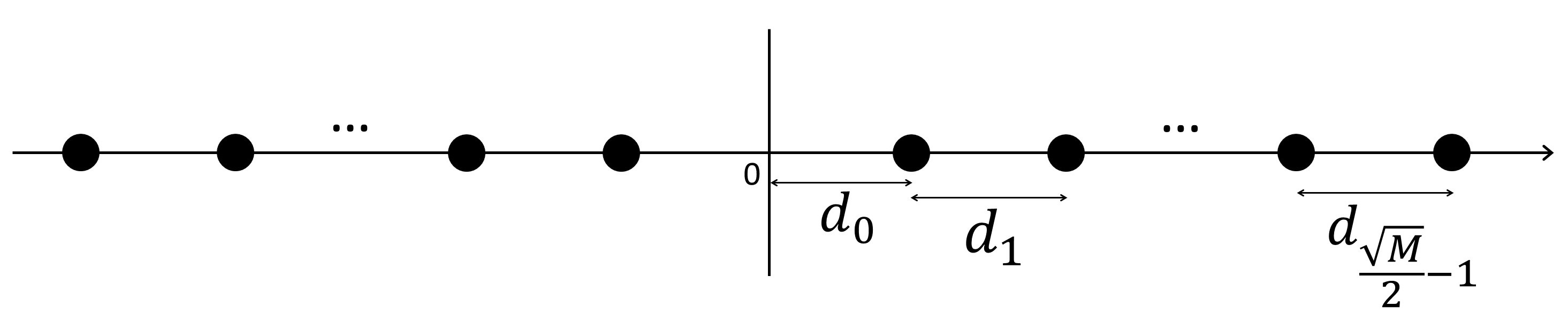
Figure 2: Normalized PAM constellation design for the RIS-RQSM system.

The expression for $\mathrm{ABEP}_{\mathrm{ub}}$ in (18) is a relatively complex function of the parameters $\left\{d_{i}\right\}$ due to the summation over all symbols in calculating $P_{e}\left(m\right)$ and in calculating $\mathrm{PEP}\left(x^{\mathcal{R}}\rightarrow\hat{x}^{\mathcal{R}}|m=\hat{m}\right)$ associated with all of these distances. Hence, to simplify the solution for the optimization problem in (29) we adopt some accurate approximations for evaluating the upper bound on the ABEP that are valid at high SNR and with large $N$.

It is well-known that at high SNR values the IQ modulation domain bit error probability (BEP) is dominated by the pairs of constellation points separated by the minimum Euclidean distance, and it is also clear that the minimum-energy symbols control the BEP in the spatial domain. Hence, considering Gray coding for the constellation, an approximate upper bound on the ABEP is given by

$$\mathrm{ABEP}_{\mathrm{ub}}\approx\frac{4}{\sqrt{M}\log_{2}\left(\sqrt{M}N_{r}\right)}\sum_{i=1}^{\frac{\sqrt{M}}{2}-1}\mathrm{Q}\left(\sqrt{\frac{\beta^{2}E_{s}d_{i}^{2}}{2N_{0}}}\right)+0.5\tilde{P}_{e}\left(m\right),$$ (30)

where $\tilde{P}_{e}\left(m\right)$ is the corresponding approximate value of $P_{e}\left(m\right)$, given by

$$\tilde{P}_{e}\left(m\right)=\frac{4\left(N_{r}-1\right)}{M}\sum_{\delta\in\mathcal{D}_{d_{0}\sqrt{E_{s}}}}\mathrm{PEP}\left(m\rightarrow\hat{m}|x^{\mathcal{R}}=d_{0}\sqrt{E_{s}},\delta\right),$$ (31)

where $\mathcal{D}_{d_{0}\sqrt{E_{s}}}=\Bigl{\{}1,\frac{d_{0}}{d_{0}+d_{1}},\dots,\frac{d_{0}}{d_{0}+d_{1}+\cdots+d_{\frac{\sqrt{M}}{2}-1}}\Bigr{\}}$, and we use the fact that $\tilde{P}_{e}\left(m\right)\ll 1$, hence $1-\tilde{P}_{e}\left(m\right)\approx 1$ (note that the optimization function increases the distance between two inner symbols, so that in (30), we did not consider the distance between the pair of inner symbols as the minimum distance). Then, the optimization problem can be updated as

$$\underset{\left\{d_{i}\right\}}{\min} \ \mathrm{ABEP}_{\mathrm{ub}}\mbox{ in (\ref{eq:Approx_ABEP})}$$ (32)

s.t. $$\ \sum_{i=0}^{\frac{\sqrt{M}}{2}-1}\left(\sum_{j=0}^{i}d_{j}\right)^{2}\leq\frac{\sqrt{M}}{4}.$$

Solving the above optimization problem is not a straightforward task and requires the use of exhaustive search methods. However, standard lattice constellation structures, such as QAM or PAM, suggest that equal distances between adjacent pairs of symbols admit a very simple approach which provides a near-optimal solution in terms of the symbol error rate performance. Hence, in the following, we assume that the distances between “positive” adjacent symbols are equal (it is worth recalling that there is a symmetry about the origin, hence the distances between negative adjacent symbols are also equal).

Special case where $d_{1}=d_{2}=\dots=d_{\frac{\sqrt{M}}{2}-1}$

In this case, the problem consists of optimizing the two variables $d_{0}$ and $d_{1}$. Hence, the optimization problem reduces to

$$\underset{\left\{d_{0},d_{1}\right\}}{\min} \ \frac{4}{\sqrt{M}\log_{2}\left(\sqrt{M}N_{r}\right)}M^{\prime}\mathrm{Q}\left(\sqrt{\frac{\beta^{2}E_{s}d_{1}^{2}}{2N_{0}}}\right)+0.5\tilde{P}_{e}\left(m\right),$$ (33)

s.t. $$\ 2d_{0}^{2}+\frac{M^{\prime}\left(2M^{\prime}+1\right)}{3}d_{1}^{2}+2M^{\prime}d_{0}d_{1}\leq 1,$$

where we define $M^{\prime}=\frac{\sqrt{M}}{2}-1.$ From the inequality constraint, $d_{1}$ can be obtained as a function of $d_{0}$ (here we force equality in the constraint above to maximize the achievable SNR at the receiver. It will be shown later in this section that equality indeed holds at the optimum point). Then, by performing a grid search over variable $d_{0}$, we can find the minimum value of the $\mathrm{ABEP}_{\mathrm{ub}}$. However, taking the equal positive distance into account, it is more valuable to find an analytical solution; this is the subject of the remainder of this section.

Analytical approach - asymptotic analysis

In order to find an efficient analytical solution for the optimization problem, we analyze the distributions of $Z_{1}$ and $Z_{2}$ in more detail in order to obtain a more tractable approximate expression for $\mathrm{ABEP}_{\mathrm{ub}}$. We see that the variance of $Z_{2}$ (i.e., the average received energy of the signal on a non-selected receive antenna) in the event $\mathcal{E}_{1}$ increases with decreasing $\bar{\lambda}=\frac{\delta^{2}}{1+\delta^{2}}$, or equivalently, with decreasing $\delta=\left|\frac{x^{\mathcal{R}}}{x^{\mathcal{I}}}\right|$; in other words, $\rho_{1}^{2}$ in (22) is maximized when $\delta$ is minimized. There are two consequences of this fact: first, the BEP related to the spatial domain is dominated by those symbols bearing the minimum energy in the real part while their corresponding imaginary parts have the maximum energy, i.e., the PEP associated with $\delta_{\min}=\frac{\min\left|x^{\mathcal{R}}\right|}{\max\left|x^{\mathcal{I}}\right|}=\frac{d_{0}}{d_{0}+M^{\prime}d_{1}}$ dominates (31); secondly, comparing the two events $\mathcal{E}_{1}$ and $\mathcal{E}_{2}$, the event $\mathcal{E}_{2}$ has a minor impact on the value of $\mathrm{PEP}\left(m\rightarrow\hat{m}|x^{\mathcal{R}},\delta\right)$, as the variance of $Z_{2}$ in the event $\mathcal{E}_{1}$ is significantly greater than that in the event $\mathcal{E}_{2}$ due to the appearance of $\bar{\lambda}$ in the denominator. In summary, considering the above comments, the PEP associated to $\delta_{\min}$ dominates and the event $\mathcal{E}_{2}$ can be eliminated from the PEP analysis, therefore $\tilde{P}_{e}\left(m\right)$ can be approximated as

$$\tilde{P}_{e}\left(m\right) \approx\frac{4\left(N_{r}-1\right)}{M}\mathrm{PEP}\left(m\rightarrow\hat{m}|x^{\mathcal{R}}=d_{0}\sqrt{E_{s}},\delta=\delta_{\min}\right)$$

$$\approx\frac{4\left(N_{r}-1\right)^{2}}{MN_{r}}\mathrm{I}_{1}\left(\mu_{1},\rho_{1},\sigma_{1}\right).$$ (34)

In addition, by substituting $\bar{\lambda}=\frac{\delta_{\min}^{2}}{1+\delta_{\min}^{2}}$ into (22) and performing some minor algebraic manipulations, the variance of $Z_{2}$ in the event $\mathcal{E}_{1}$ can be expressed as

$$\rho_{1}^{2}=\frac{NE_{s}}{2}\left(d_{0}^{2}+\left(d_{0}+M^{\prime}d_{1}\right)^{2}\right)+\frac{N_{0}}{2}.$$

Note that $\bar{E}\triangleq d_{0}^{2}+\left(d_{0}+M^{\prime}d_{1}\right)^{2}$ is the sum of the energies associated with the symbols with minimum and maximum distance from the origin. It is clear that $1\leq\bar{E}<\epsilon_{M}$, where equality holds for $M=16$, and $\epsilon_{M}$ is defined as the total energy of the inner and outer symbols in the conventional $\sqrt{M}$-PAM constellation (since the conventional constellation is the worst-case scenario, $\bar{E}$ can be upper bounded by $\epsilon_{M}$), so that we obtain $\epsilon_{M}=\frac{3(M-2\sqrt{M}+2)}{2(M-1)}$ (note that the average energy of the PAM constellation is $1/2$). Therefore, we can write

$$\frac{NE_{s}}{2}+\frac{N_{0}}{2}\leq\rho_{1}^{2}<\frac{NE_{s}}{2}\epsilon_{M}+\frac{N_{0}}{2}.$$

In addition, it is easy to prove that (34) is monotonically increasing with respect to $\rho_{1}$. Hence, $\tilde{P}_{e}\left(m\right)$ can be expressed as

$$\tilde{P}_{e}\left(m\right) \approx\left.\tilde{P}_{e}\left(m\right)\right|_{\rho_{1}^{2}=\frac{NE_{s}}{2}+\frac{N_{0}}{2}},\ M=16,$$

$$\tilde{P}_{e}\left(m\right) \lesssim\left.\tilde{P}_{e}\left(m\right)\right|_{\rho_{1}^{2}=\frac{NE_{s}}{2}\epsilon_{M}+\frac{N_{0}}{2}},\ M>16.$$

Finally, from the formula $\sigma_{1}^{2}=N\left(x^{\mathcal{R}}\right)^{2}\frac{4-\pi}{4}+\frac{N_{0}}{2}$ applied to the minimum energy symbol $x^{\mathcal{R}}=d_{0}\sqrt{E_{s}}$ and considering the fact that $d_{0}^{2}\ll 1$, the variance of $Z_{1}$ can be approximated as $\sigma_{1}^{2}\approx\frac{N_{0}}{2}$.

Therefore, after some manipulations we obtain $\tilde{P}_{e}\left(m\right)$ as

$$\tilde{P}_{e}\left(m\right)\approx \frac{2\left(N_{r}-1\right)^{2}}{MN_{r}}\left(\frac{1}{3}\sqrt{\frac{NE_{s}+N_{0}}{NE_{s}+2N_{0}}}e^{-\frac{\pi N^{2}E_{s}d_{0}^{2}}{4NE_{s}+8N_{0}}}+\sqrt{\frac{NE_{s}+N_{0}}{NE_{s}+\frac{7}{3}N_{0}}}e^{-\frac{\pi N^{2}E_{s}d_{0}^{2}}{3NE_{s}+7N_{0}}}\right),\ M=16,$$

$$\tilde{P}_{e}\left(m\right)\lesssim \frac{2\left(N_{r}-1\right)^{2}}{MN_{r}}\left(\frac{1}{3}\sqrt{\frac{NE_{s}\epsilon_{M}+N_{0}}{NE_{s}\epsilon_{M}+2N_{0}}}e^{-\frac{\pi N^{2}E_{s}d_{0}^{2}}{4NE_{s}\epsilon_{M}+8N_{0}}}+\sqrt{\frac{NE_{s}\epsilon_{M}+N_{0}}{NE_{s}\epsilon_{M}+\frac{7}{3}N_{0}}}e^{-\frac{\pi N^{2}E_{s}d_{0}^{2}}{3NE_{s}\epsilon_{M}+7N_{0}}}\right),$$

$$M>16.$$

Also applying the exponential approximation of the Q-function in (33), the optimization problem becomes

$$\underset{\left\{d_{0},d_{1}\right\}}{\min} \ \mathrm{ABEP}_{\mathrm{ub}}\approx a_{0}e^{-b_{0}d_{0}^{2}}+a_{1}e^{-b_{1}d_{0}^{2}}+M^{\prime}a_{2}\left(\frac{1}{12}e^{-b_{2}d_{1}^{2}}+\frac{1}{4}e^{-\frac{4}{3}b_{2}d_{1}^{2}}\right)$$ (35)

s.t. $$\ 2d_{0}^{2}+\frac{M^{\prime}\left(2M^{\prime}+1\right)}{3}d_{1}^{2}+2M^{\prime}d_{0}d_{1}\leq 1,$$

where we define

$$a_{0}=\frac{\left(N_{r}-1\right)^{2}}{3MN_{r}}\sqrt{\frac{NE_{s}\epsilon_{M}+N_{0}}{NE_{s}\epsilon_{M}+2N_{0}}},\;b_{0}=\frac{\pi N^{2}E_{s}}{4NE_{s}\epsilon_{M}+8N_{0}},$$

$$a_{1}=\frac{\left(N_{r}-1\right)^{2}}{MN_{r}}\sqrt{\frac{NE_{s}\epsilon_{M}+N_{0}}{NE_{s}\epsilon_{M}+\frac{7}{3}N_{0}}},\;b_{1}=\frac{\pi N^{2}E_{s}}{3NE_{s}\epsilon_{M}+7N_{0}},$$

$$a_{2}=\frac{4}{\sqrt{M}\log_{2}\left(\sqrt{M}N_{r}\right)},\ b_{2}=\frac{\pi N^{2}E_{s}}{16N_{0}}.$$

The problem in (35) is not a convex optimization problem, as the objective function is not convex in the domain of $d_{0},d_{1}\in\mathbb{R}_{+}$. However, it is easy to see that (35) satisfies the convexity condition $\nabla^{2}\mathrm{ABEP_{ub}}\geq 0$ when $d_{0}\geq\frac{1}{\sqrt{2b_{i}}}$, $i=0,1$, and $d_{1}\geq\frac{1}{\sqrt{2b_{2}}}$. For sufficiently high values of $\frac{N^{2}E_{s}}{N_{0}}$ (note that $N\gg 1$), it can be concluded that $\left\{b_{0},b_{1},b_{2}\right\}$ are sufficiently large such that the optimized $\left\{d_{0},d_{1}\right\}$ lie in the convex region of the objective function. For such $\left\{b_{0},b_{1},b_{2}\right\}$, the problem is convex and can be solved using the following procedure.

The Karush-Kuhn-Tucker (KKT) [29] conditions associated to the above problem hold and are given by

$$1.\;f_{1}\left(d_{0}^{\star},d_{1}^{\star}\right)\leq 0;\quad 2.\;\nu^{\star}\geq 0;\quad 3.\;\nu^{\star}f_{1}\left(d_{0}^{\star},d_{1}^{\star}\right)=0;$$

$$4.\;-2a_{0}b_{0}d_{0}^{\star}e^{-b_{0}d_{0}^{\star^{2}}}-2a_{1}b_{1}d_{0}^{\star}e^{-b_{1}d_{0}^{\star^{2}}}+\nu^{\star}\left(4d_{0}^{\star}+2M^{\prime}d_{1}^{\star}\right)=0;$$

$$5.\;-\frac{1}{6}M^{\prime}a_{2}b_{2}d_{1}^{\star}e^{-b_{2}d_{1}^{\star^{2}}}-\frac{2}{3}M^{\prime}a_{2}b_{2}d_{1}^{\star}e^{-\frac{4}{3}b_{2}d_{1}^{\star^{2}}}+\nu^{\star}\left(\frac{2M^{\prime}\left(2M^{\prime}+1\right)}{3}d_{1}^{\star}+2M^{\prime}d_{0}^{\star}\right)=0;$$

where $\nu$ is the Lagrange multiplier associated with the inequality constraint. From condition 3, we see that $\nu^{\star}=0$ or $f_{1}\left(d_{0}^{\star},d_{1}^{\star}\right)=0$. However, if $\nu^{\star}=0$, from conditions 4 and 5 we obtain $d_{0}^{\star}=d_{1}^{\star}=+\infty$, where clearly contradicts condition 1. Therefore, we have

$$2d_{0}^{\star^{2}}+\frac{M^{\prime}\left(2M^{\prime}+1\right)}{3}d_{1}^{\star^{2}}+2M^{\prime}d_{0}^{\star}d_{1}^{\star}-1=0,$$

which yields

$$d_{0}^{\star}=\frac{-2M^{\prime}d_{1}^{\star}+\sqrt{4M^{\prime^{2}}d_{1}^{\star^{2}}-8\left(\frac{M^{\prime}\left(2M^{\prime}+1\right)}{3}d_{1}^{\star^{2}}-1\right)}}{4}.$$ (36)

Then, from conditions 4 and 5, we obtain

$$\nu^{\star}=a_{0}b_{0}d_{0}^{\star^{2}}e^{-b_{0}d_{0}^{\star^{2}}}+a_{1}b_{1}d_{0}^{\star^{2}}e^{-b_{1}d_{0}^{\star^{2}}}+\frac{1}{12}M^{\prime}a_{2}b_{2}d_{1}^{\star^{2}}e^{-b_{2}d_{1}^{\star^{2}}}+\frac{1}{3}M^{\prime}a_{2}b_{2}d_{1}^{\star^{2}}e^{-\frac{4}{3}b_{2}d_{1}^{\star^{2}}}.$$ (37)

Substituting for $\nu^{\star}$ from (37) and subsequently for $d_{0}^{\star}$ from (36) into condition 5, the optimization problem reduces to a single-variable equation in $d_{1}^{\star}$. This equation does not admit a closed-form analytical solution; however it is easy to solve numerically.

We conclude this section by providing a numerical example in Table I. In this table, we compare the optimal $\{d_{i}\}$ obtained by an exhaustive search to minimize the ABEP in (18) with the corresponding values with equal positive distances obtained via the proposed analytical approach, where $N=256$, $N_{r}=4$ and $M=64$. It can be seen that positive distances $\{d_{i}\}$, $i>0$, obtained via exhaustive search are almost equal, and that these values become more similar with increasing SNR. In addition, the ABEP values acquired by using the optimal values from the proposed analytical approach are quite comparable to the equivalent ABEP obtained by optimal values of the grid search, which serves as a proof that the assumptions we made to offer a straightforward analytical solution to the optimization problem were indeed accurate.

TABLE I: Comparison between optimal $\{d_{i}\}$ values obtained via minimizing (18) by grid search and the corresponding values obtained by the analytical approach of (35), where $N=256$, $N_{r}=4$ and $M=64$.

Minimized ABEP based on (18) using grid search						Minimized ABEP by using analytical approach of (35)
SNR (dB)	$d_{0}$	$d_{1}$	$d_{2}$	$d_{3}$	ABEP	$d_{0}$	$d_{1}$	ABEP
-23	0.2609	0.250	0.257	0.272	$6.97\times 10^{-4}$	0.2481	0.2632	$7.62\times 10^{-4}$
-21	0.2695	0.248	0.253	0.262	$6.46\times 10^{-5}$	0.2661	0.2543	$6.67\times 10^{-5}$
-19	0.2890	0.240	0.243	0.248	$2.90\times 10^{-6}$	0.2891	0.2426	$2.96\times 10^{-6}$
-17	0.3169	0.227	0.228	0.232	$5.71\times 10^{-8}$	0.3179	0.2278	$5.82\times 10^{-8}$

VII Numerical Results

In this section, we demonstrate the error rate performance of the proposed RIS-RQSM system via numerical simulations. First, we investigate the performance of the proposed RIS-RQSM system using conventional QAM constellations and provide comparisons with corresponding systems using QAM constellations that are optimized based on the approach proposed in Section VI. Next, we compare the results obtained by the optimized constellations with the error rate performance of the most prominent recently proposed RIS-SM [14] system, which serves as the benchmark scheme for the proposed approach.

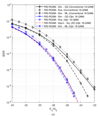
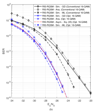
Figure 3: Analytical and simulation BER results of the proposed RIS-RQSM system with and without optimized constellation. Here $M=16$, $N=256$, and (a) $N_{r}=4$ ($R=8$ bpcu), (b) $N_{r}=8$ ($R=10$ bpcu).

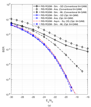
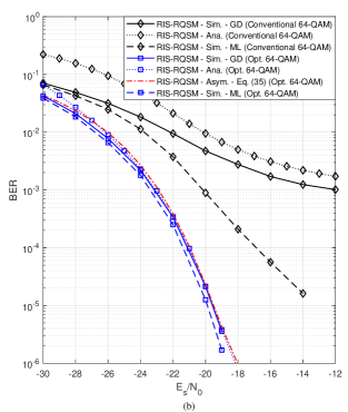
Figure 4: Analytical and simulation BER results of the proposed RIS-RQSM system with and without optimized constellation. Here $M=64$, $N=256$, and (a) $N_{r}=4$ ($R=10$ bpcu), (b) $N_{r}=8$ ($R=12$ bpcu).

Fig. 3 shows the BER performance of the proposed RIS-RQSM system with $N=256$ for the cases of $N_{r}=4$ and $N_{r}=8$. In this figure, we also compare the performance of the RIS-RQSM system using conventional 16-QAM modulation with that of the system implementing our optimized 16-QAM constellation. The curves demonstrate the effectiveness of the proposed constellation design method; it can be observed that optimizing the design of the constellation significantly enhances the performance of the system. The proposed constellation for RIS-RQSM provides approximately 3.2 dB and 3.8 dB improvement over the conventional constellation in systems with $N_{r}=4$ and $N_{r}=8$, respectively, at a BER of $10^{-5}$. We also compare the performance of the GD with that of the ML detector. We see that there is a very large gap between the performance of the GD and ML detector in the case of the conventional constellation, while the performance of the GD in the system using the optimized constellation is considerably close to that of the ML detector such that the performance gap is negligible. In order to observe the effect of optimizing the constellation in a system with higher-order modulation, we present the BER performance of the RIS-RQSM system with 64-QAM in Fig. 4. Here, we see that in systems with regular QAM constellations, an error floor occurs with the GD. This is due to the fact that with critical symbols, i.e., minimum-energy symbols, $\bar{\lambda}$ can attain a very small value; hence, non-selected antennas can have a relatively high average received energy compared to the selected antenna. However, we see that optimizing the constellation eliminates this error floor and substantially improves the error rate performance. Similar to systems with 16-QAM constellation, the performance of the GD is very close to that of ML detector with optimized constellations. In fact, here the GD becomes feasible only with the optimized 64-QAM. In Figs. 3 and 4, we also present the analytical ABEP performance of each system. For systems with conventional QAM constellations, we evaluate and plot the analytical ABEP upper bounds based on (18); we see that upper bound curves are quite tight and validate the accuracy of the analytical results. For systems with optimized constellation we also plot the asymptotic result in (35). These curves show that the utilized approximations in Section VI are completely valid and accurate, especially at high SNR.

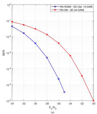
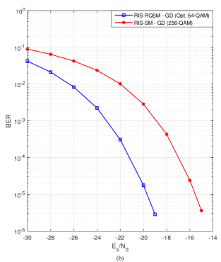
Figure 5: Comparison of the BER performance of the proposed RIS-RQSM system with that of RIS-SM system for $N=256$, $N_{r}=4$, and (a) $R=8$ bpcu, (b) $R=10$ bpcu.

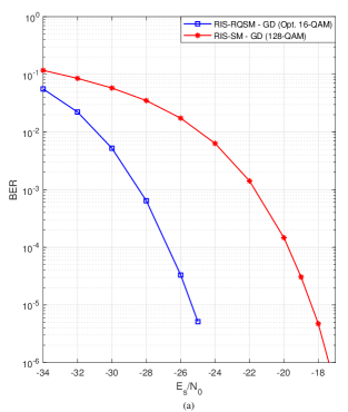
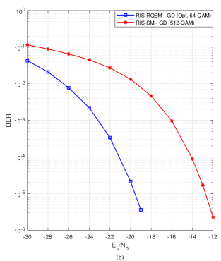
Figure 6: Comparison of the BER performance of the proposed RIS-RQSM system with that of RIS-SM system for $N=256$, $N_{r}=8$, and (a) $R=10$ bpcu, (b) $R=12$ bpcu.

Next, in Fig. 5, we compare the BER performance of the proposed RIS-RQSM system with that of the benchmark scheme, i.e., RIS-SM, in systems with $N=256$ and $N_{r}=4$. Fig. 5(a) shows the performance of the RIS-RQSM and RIS-SM systems where the bit rate is $R=8$ bpcu. Hence, the proposed RIS-RQSM system uses 16-QAM modulation, while the RIS-SM system uses 64-QAM modulation. The constellation used in the proposed RIS-RQSM system is optimized to achieve the best performance. Fig. 5(b) presents the performance results in systems with $R=10$ bpcu, i.e., where RIS-RQSM and RIS-SM apply 64-QAM and 256-QAM, respectively. The results show that the proposed RIS-RQSM system substantially outperforms the benchmark scheme. This is mainly due to the fact that the RIS-SM system needs to employ a higher-order modulation technique in order to compensate the additional bits transmitted by the quadrature index modulation in the proposed RIS-RQSM system. Hence, the superiority over the benchmark scheme increases by increasing number of receive antennas, as shown in Fig. 6. In this figure, we provide comparisons between the BER performance of the RIS-RQSM and RIS-SM systems where $N=256$ and $N_{r}=8$. As expected, the superiority over the RIS-SM system considerably increases in a system with larger number of receive antennas, as a higher modulation order is required for the RIS-SM system. The proposed RIS-RQSM system achieves approximately 4.3 dB and 7 dB performance improvement over the RIS-SM system for systems with $N_{r}=4$ and $N_{r}=8$, respectively, at a BER of $10^{-5}$. It is worth pointing out that the receiver in the proposed RIS-RQSM system requires minimal CSI due to the use of the pre-equalizer $G$; this CSI consists only of the average gain of the effective channel, which is simply a function of the number of RIS elements, as shown in Section II.

VIII Conclusion

The RIS-assisted receive quadrature spatial modulation (RIS-RQSM) system was proposed in this paper as a general approach to RIS-assisted receive SM with excellent performance. The proposed system increases the spectral efficiency by implementing both quadrature spatial modulation and IQ modulation, while maintaining the signal quality at the receiver. In the proposed RIS-RQSM system, the phase shifts of the RIS elements are designed to construct an IQ symbol at the receiver; this enables the system to transmit two separate PAM symbols in the presence of the RIS. We introduced a one-tap pre-equalizer to allow the proposed low-complexity GD to detect the symbols with minimum CSI requirement. Analytical results and numerical simulations both verify the excellent performance of the system and extensively demonstrate its superiority over comparable benchmark schemes in the literature. The many advantages of the RIS-RQSM system makes it a viable candidate for next-generation wireless communication networks.

Appendix A Proof of Theorem 1

Here we analyze the average of

$$Y_{R}^{\star}=\text{sgn}\left(x^{\mathcal{R}}\right)\left(\mathbf{h}_{m}^{\mathcal{R}}\boldsymbol{\theta}^{\mathcal{R}\star}-\mathbf{h}_{m}^{\mathcal{I}}\boldsymbol{\theta}^{\mathcal{I}\star}\right)=\sum_{i=1}^{N}\frac{\lambda A_{i}^{2}+\lambda C_{i}^{2}+\left(1-\lambda\right)A_{i}B_{i}+\left(1-\lambda\right)C_{i}D_{i}}{\sqrt{\left(\lambda A_{i}+\left(1-\lambda\right)B_{i}\right)^{2}+\left(\lambda C_{i}+\left(1-\lambda\right)D_{i}\right)^{2}}}.$$

As stated before, for large values of $N$, we have $\mathbb{V}\left\{\lambda\right\}\approx 0$; therefore, we replace $\lambda$ by $\bar{\lambda}$ in calculating the average of $Y_{R}^{\star}$; this yields

$$\mathbb{E}\left\{Y_{R}^{\star}\right\} \approxeq\mathbb{E}\left\{\sum_{i=1}^{N}\frac{\bar{\lambda}A_{i}^{2}+\bar{\lambda}C_{i}^{2}+\left(1-\bar{\lambda}\right)A_{i}B_{i}+\left(1-\bar{\lambda}\right)C_{i}D_{i}}{\sqrt{\left(\bar{\lambda}A_{i}+\left(1-\bar{\lambda}\right)B_{i}\right)^{2}+\left(\bar{\lambda}C_{i}+\left(1-\bar{\lambda}\right)D_{i}\right)^{2}}}\right\}$$

$$=N\mathbb{E}\left\{\frac{\bar{\lambda}A_{i}^{2}+\bar{\lambda}C_{i}^{2}+\left(1-\bar{\lambda}\right)A_{i}B_{i}+\left(1-\bar{\lambda}\right)C_{i}D_{i}}{\sqrt{\left(\bar{\lambda}A_{i}+\left(1-\bar{\lambda}\right)B_{i}\right)^{2}+\left(\bar{\lambda}C_{i}+\left(1-\bar{\lambda}\right)D_{i}\right)^{2}}}\right\},$$

where we used the fact that each of the summands has an identical distribution. In the following, we evaluate the average of the terms in the above summation individually and we omit the index $i$ to simplify the notation; hence we define

$$W_{1}\triangleq\bar{\lambda}\frac{A^{2}}{\sqrt{Z}},\;W_{2}\triangleq\bar{\lambda}\frac{C^{2}}{\sqrt{Z}},\;W_{3}\triangleq\left(1-\bar{\lambda}\right)\frac{AB}{\sqrt{Z}},\;W_{4}\triangleq\left(1-\bar{\lambda}\right)\frac{CD}{\sqrt{Z}},$$

where $Z\triangleq\left(\bar{\lambda}A+\left(1-\bar{\lambda}\right)B\right)^{2}+\left(\bar{\lambda}C+\left(1-\bar{\lambda}\right)D\right)^{2}$.

According to the law of total expectation, the expected value of $W_{1}$ can be expressed as

$$\mathbb{E}\left\{W_{1}\right\}=\mathbb{E}_{A}\left\{\mathbb{E}_{W_{1}|A}\left\{W_{1}|A\right\}\right\}=\bar{\lambda}\mathbb{E}_{A}\left\{A^{2}\mathbb{E}_{Z|A}\left\{Z^{-\frac{1}{2}}|A\right\}\right\},$$ (38)

where $\mathbb{E}_{Z|A}\left\{Z^{-\frac{1}{2}}|A\right\}$ is the inverse-fractional moment of $Z$ where $A$ is given, i.e., where $A$ is a constant. For a given $A$, using $\bar{\lambda}=\frac{\delta^{2}}{1+\delta^{2}}$ we have $\left(\bar{\lambda}A+\left(1-\bar{\lambda}\right)B\right)\sim\mathcal{N}\left(\bar{\lambda}A,\frac{\bar{\lambda}\left(1-\bar{\lambda}\right)}{2}\right)$, and $\left(\bar{\lambda}C+\left(1-\bar{\lambda}\right)D\right)\sim\mathcal{N}\left(0,\frac{\bar{\lambda}}{2}\right)$. Hence, the random variable (RV) $(Z|A)$ is the sum of two independent chi-square RVs each having one degree of freedom. The inverse-fractional moment of $\left(Z|A\right)$ can be computed by using the following equation [30]

$$\mathbb{E}_{Z|A}\left\{Z^{-c}|A\right\}=\frac{1}{\Gamma\left(c\right)}\int_{0}^{\infty}s^{c-1}\mathbb{E}_{Z|A}\left\{e^{-sZ}|A\right\}\mathrm{d}s,$$ (39)

where $\mathbb{E}_{Z|A}\left\{e^{-sZ}|A\right\}=\mathcal{L}_{s}\left(f_{Z}\left(Z|A\right)\right)$ is the Laplace transform (LT) of $f_{Z}\left(Z|A\right)$. We know that the LT of the probability density function (PDF) of the sum of independent RVs is equal to the product of the LTs of their individual PDFs, and that the LT of the PDF of an RV $X=\sum_{i=1}^{n}X_{i}^{2}$ with $X_{i}\sim\mathcal{N}\left(\mu_{i},\sigma^{2}\right)$ is given by

$$\mathcal{L}_{s}\left(f_{X}(X)\right)=\left(\frac{1}{1+2\sigma^{2}s}\right)^{\frac{n}{2}}\exp\left(\frac{-\mu^{2}s}{1+2\sigma^{2}s}\right),$$ (40)

where $\mu^{2}=\sum_{i=1}^{n}\mu_{i}^{2}$. Hence, the LT of $f_{Z}\left(Z|A\right)$ is calculated as

$$\mathcal{L}_{s}\left(f_{Z}\left(Z|A\right)\right)=\left(\frac{1}{1+\bar{\lambda}s}\right)^{\frac{1}{2}}\left(\frac{1}{1+\bar{\lambda}\left(1-\bar{\lambda}\right)s}\right)^{\frac{1}{2}}\exp\left(\frac{-\bar{\lambda}^{2}A^{2}s}{1+\bar{\lambda}\left(1-\bar{\lambda}\right)s}\right).$$ (41)

Then, (38) can be written as

$$\mathbb{E}\left\{W_{1}\right\}= \frac{\bar{\lambda}}{\Gamma^{2}\left(\frac{1}{2}\right)}\int_{0}^{\infty}s^{\frac{1}{2}-1}\left(\frac{1}{1+\bar{\lambda}s}\right)^{\frac{1}{2}}\left(\frac{1}{1+\bar{\lambda}\left(1-\bar{\lambda}\right)s}\right)^{\frac{1}{2}}$$

$$\times\left(\int_{-\infty}^{\infty}A^{2}\exp\left(-A^{2}\frac{1+\bar{\lambda}s}{1+\bar{\lambda}\left(1-\bar{\lambda}\right)s}\right)\mathrm{d}A\right)\mathrm{d}s,$$

where we used the fact that $f_{A}\left(A\right)=\frac{1}{\Gamma\left(\frac{1}{2}\right)}\exp\left(-A^{2}\right)$. Since $\int_{-\infty}^{\infty}x^{2}\exp\left(-\frac{x^{2}}{2\sigma^{2}}\right)\mathrm{d}x=\Gamma\left(\frac{1}{2}\right)\sigma^{2}\sqrt{2\sigma^{2}}$, we have

$$\int_{-\infty}^{\infty}A^{2}\exp\left(-A^{2}\frac{1+\bar{\lambda}s}{1+\bar{\lambda}\left(1-\bar{\lambda}\right)s}\right)\mathrm{d}A=\frac{\Gamma\left(\frac{1}{2}\right)}{2}\left(\frac{1+\bar{\lambda}\left(1-\bar{\lambda}\right)s}{1+\bar{\lambda}s}\right)^{\frac{3}{2}}.$$

It follows that

$$\mathbb{E}\left\{W_{1}\right\} =\bar{\lambda}\frac{1}{2\Gamma\left(\frac{1}{2}\right)}\int_{0}^{\infty}s^{\frac{1}{2}-1}\frac{1+\bar{\lambda}\left(1-\bar{\lambda}\right)s}{\left(1+\bar{\lambda}s\right)^{2}}\mathrm{d}s$$

$$=\bar{\lambda}\left(1-\bar{\lambda}\right)\frac{1}{2\Gamma\left(\frac{1}{2}\right)}\left(\int_{0}^{\infty}s^{\frac{1}{2}-1}\left(1+\bar{\lambda}s\right)^{-1}\mathrm{d}s+\frac{\bar{\lambda}}{1-\bar{\lambda}}\int_{0}^{\infty}s^{\frac{1}{2}-1}\left(1+\bar{\lambda}s\right)^{-2}\mathrm{d}s\right).$$

Recalling the definition of the type-2 beta function $\mathrm{B}\left(\alpha,\beta\right)=\int_{0}^{\infty}\frac{t^{\alpha-1}}{\left(1+t\right)^{\alpha+\beta}}\mathrm{d}t=\frac{\Gamma\left(\alpha\right)\Gamma\left(\beta\right)}{\Gamma\left(\alpha+\beta\right)}$, after some minor manipulations we obtain

$$\mathbb{E}\left\{W_{1}\right\}=\bar{\lambda}^{\frac{1}{2}}\left(1-\bar{\lambda}\right)\frac{1}{2\Gamma\left(\frac{1}{2}\right)}\left(\frac{\Gamma\left(\frac{1}{2}\right)\Gamma\left(\frac{1}{2}\right)}{\Gamma\left(1\right)}+\frac{\bar{\lambda}}{1-\bar{\lambda}}\frac{\Gamma\left(\frac{1}{2}\right)\Gamma\left(\frac{3}{2}\right)}{\Gamma\left(2\right)}\right)=\frac{\sqrt{\pi}}{4}\left(2\bar{\lambda}^{\frac{1}{2}}-\bar{\lambda}^{\frac{3}{2}}\right).$$

By symmetry it is clear that $\mathbb{E}\left\{W_{2}\right\}=\mathbb{E}\left\{W_{1}\right\}$.

Next we determine $\mathbb{E}\left\{W_{3}\right\}=\mathbb{E}\left\{\left(1-\bar{\lambda}\right)\frac{AB}{\sqrt{Z}}\right\}$. Using the law of total expectation, we can write

$$\mathbb{E}\left\{W_{3}\right\} =\left(1-\bar{\lambda}\right)\mathbb{E}_{A}\left\{A\mathbb{E}_{B}\left\{B\mathbb{E}_{Z|(A,B)}\left\{Z^{-\frac{1}{2}}|(A,B)\right\}\right\}\right\}.$$

Given constant $(A,B)$, we have

$$\mathcal{L}_{s}\left(f_{Z}\left(Z|(A,B)\right)\right)=\left(\frac{1}{1+\bar{\lambda}s}\right)^{\frac{1}{2}}\exp\left(-\left(\bar{\lambda}A+\left(1-\bar{\lambda}\right)B\right)^{2}s\right).$$ (42)

Using (39), we have

$$\mathbb{E}\left\{W_{3}\right\}=\left(1-\bar{\lambda}\right)\mathbb{E}_{A}\Biggl{\{}A\mathbb{E}_{B}\Biggl{\{}\frac{B}{\Gamma\left(\frac{1}{2}\right)}\int_{0}^{\infty}s^{\frac{1}{2}-1}\left(\frac{1}{1+\bar{\lambda}s}\right)^{\frac{1}{2}}\exp\left(-\left(\bar{\lambda}A+\left(1-\bar{\lambda}\right)B\right)^{2}s\right)ds\Biggr{\}}\Biggr{\}}.$$

Then, using $f_{A}\left(A\right)=\frac{1}{\Gamma\left(\frac{1}{2}\right)}\exp\left(-A^{2}\right)$ and $f_{B}\left(B\right)=\frac{\left(1-\bar{\lambda}\right)^{\frac{1}{2}}}{\bar{\lambda}^{\frac{1}{2}}\Gamma\left(\frac{1}{2}\right)}\exp\left(-\frac{1-\bar{\lambda}}{\bar{\lambda}}B^{2}\right)$, after some algebraic manipulations we obtain

$$\mathbb{E}\left\{W_{3}\right\}= \frac{\left(1-\bar{\lambda}\right)^{\frac{3}{2}}}{\bar{\lambda}^{\frac{1}{2}}}\frac{1}{\Gamma^{3}\left(\frac{1}{2}\right)}\int_{0}^{\infty}s^{\frac{1}{2}-1}\left(\frac{1}{1+\bar{\lambda}s}\right)^{\frac{1}{2}}$$

$$\times\left[\int_{-\infty}^{\infty}A\exp\left(-A^{2}\frac{1+\bar{\lambda}s}{1+\bar{\lambda}\left(1-\bar{\lambda}\right)s}\right)\left(\int_{-\infty}^{\infty}B\exp\left(-\frac{\left(B+\frac{\bar{\lambda}^{2}As}{1+\bar{\lambda}\left(1-\bar{\lambda}\right)s}\right)^{2}}{\frac{\bar{\lambda}/(1-\bar{\lambda})}{\left(1+\bar{\lambda}\left(1-\bar{\lambda}\right)s\right)}}\right)\mathrm{d}B\right)\mathrm{d}A\right]\mathrm{d}s.$$ (43)

The inner integral over $B$ can be evaluated as

$$\int_{-\infty}^{\infty}B\exp\left(-\frac{\left(B+\frac{\bar{\lambda}^{2}As}{1+\bar{\lambda}\left(1-\bar{\lambda}\right)s}\right)^{2}}{\frac{\frac{\bar{\lambda}}{1-\bar{\lambda}}}{1+\bar{\lambda}\left(1-\bar{\lambda}\right)s}}\right)\mathrm{d}B=-\Gamma\left(\frac{1}{2}\right)\frac{\bar{\lambda}^{\frac{5}{2}}As}{\left(1-\bar{\lambda}\right)^{\frac{1}{2}}\left(1+\bar{\lambda}\left(1-\bar{\lambda}\right)s\right)^{\frac{3}{2}}}.$$

Substituting this into (43), the average of $W_{3}$ is given by

$$\mathbb{E}\left\{W_{3}\right\} =\bar{\lambda}^{2}\left(1-\bar{\lambda}\right)\frac{-1}{2\Gamma\left(\frac{1}{2}\right)}\int_{0}^{\infty}s^{\frac{3}{2}-1}\frac{1}{\left(1+\bar{\lambda}s\right)^{2}}\mathrm{d}s$$

$$=\bar{\lambda}^{\frac{1}{2}}\left(1-\bar{\lambda}\right)\frac{-1}{2\Gamma\left(\frac{1}{2}\right)}\mathrm{B}\left(\frac{3}{2},\frac{1}{2}\right)=-\frac{\sqrt{\pi}}{4}\bar{\lambda}^{\frac{1}{2}}\left(1-\bar{\lambda}\right).$$

Also, by symmetry we have $\mathbb{E}\{W_{4}\}=\mathbb{E}\{W_{3}\}$. Finally, the average of $Y_{R}^{\star}$ is given by

$$\mathbb{E}\left\{Y_{R}^{\star}\right\}\approx 2N\left(\mathbb{E}\left\{W_{1}\right\}+\mathbb{E}\left\{W_{3}\right\}\right)=\bar{\lambda}^{\frac{1}{2}}\frac{N\sqrt{\pi}}{2}.$$

Then, using $\bar{\lambda}=\frac{\delta^{2}}{1+\delta^{2}}$, $\mathbb{E}\left\{Y_{I}^{\star}\right\}$ is given by

$$\mathbb{E}\left\{Y_{I}^{\star}\right\}=\frac{1}{\delta}\mathbb{E}\left\{Y_{R}^{\star}\right\}\approx(1-\bar{\lambda})^{\frac{1}{2}}\frac{N\sqrt{\pi}}{2}.$$

References

- [1] R. Liu, Q. Wu, M. Di Renzo, and Y. Yuan, “A path to smart radio environments: An industrial viewpoint on reconfigurable intelligent surfaces,” IEEE Wireless Communications, vol. 29, pp. 202–208, Feb. 2022.
- [2] M. Di Renzo et al., “Smart radio environments empowered by reconfigurable intelligent surfaces: How it works, state of research, and the road ahead,” IEEE J. Sel. Areas Commun., vol. 38, pp. 2450–2525, Nov. 2020.
- [3] R. Alghamdi et al., “Intelligent surfaces for 6G wireless networks: A survey of optimization and performance analysis techniques,” IEEE Access, vol. 8, pp. 202795–202818, 2020.
- [4] M. Di Renzo et al., “Smart radio environments empowered by reconfigurable AI meta-surfaces: An idea whose time has come,” EURASIP J. Wireless Commun. Netw., vol. 2019, pp. 1–20, May 2019.
- [5] E. Basar, “Transmission through large intelligent surfaces: A new frontier in wireless communications,” in Proc. Eur. Conf. Netw. Commun. (EuCNC), Valencia, Spain, Jun. 2019, pp. 112–117.
- [6] E. Basar, M. Di Renzo, J. De Rosny, M. Debbah, M.-S. Alouini, and R. Zhang, “Wireless communications through reconfigurable intelligent surfaces,” IEEE Access, vol. 7, pp. 116753–116773, 2019.
- [7] R. Y. Mesleh, H. Haas, S. Sinanovic, C. W. Ahn, and S. Yun, “Spatial modulation,” IEEE Transactions on Vehicular Technology, vol. 57, pp. 2228–2241, Jul. 2008.
- [8] M. Di Renzo, H. Haas, and P. M. Grant, “Spatial modulation for multiple-antenna wireless systems: A survey,” IEEE Communications Magazine, vol. 49, pp. 182–191, Dec. 2011.
- [9] A. Younis, N. Serafimovski, R. Mesleh, and H. Haas, “Generalised spatial modulation,” in 2010 Conference Record of the Forty Fourth Asilomar Conference on Signals, Systems and Computers, pp. 1498–1502, 2010.
- [10] L.-L. Yang, “Transmitter preprocessing aided spatial modulation for multiple-input multiple-output systems,” in 2011 IEEE 73rd Vehicular Technology Conference (VTC Spring), pp. 1–5, 2011.
- [11] A. Stavridis, S. Sinanovic, M. Di Renzo, and H. Haas, “Transmit precoding for receive spatial modulation using imperfect channel knowledge,” in 2012 IEEE 75th Vehicular Technology Conference (VTC Spring), pp. 1–5, 2012.
- [12] R. Mesleh, S. S. Ikki, and H. M. Aggoune, “Quadrature spatial modulation,” IEEE Trans. Veh. Technol., vol. 64, pp. 2738–2742, Jun. 2015.
- [13] M. Di Renzo, H. Haas, A. Ghrayeb, S. Sugiura, and L. Hanzo, “Spatial modulation for generalized MIMO: Challenges, opportunities, and implementation,” Proceedings of the IEEE, vol. 102, pp. 56–103, Jan. 2014.
- [14] E. Basar, “Reconfigurable intelligent surface-based index modulation: A new beyond MIMO paradigm for 6G,” IEEE Trans. Commun., vol. 68, pp. 3187–3196, May 2020.
- [15] Q. Li, M. Wen, and M. Di Renzo, “Single-RF MIMO: From spatial modulation to metasurface-based modulation,” IEEE Wireless Communications, vol. 28, pp. 88–95, Aug. 2021.
- [16] A. E. Canbilen, E. Basar, and S. S. Ikki, “On the performance of RIS-assisted space shift keying: Ideal and non-ideal transceivers,” IEEE Transactions on Communications, vol. 70, pp. 5799–5810, Sep. 2022.
- [17] Q. Li, M. Wen, S. Wang, G. C. Alexandropoulos, and Y.-C. Wu, “Space shift keying with reconfigurable intelligent surfaces: Phase configuration designs and performance analysis,” IEEE Open J. Commun. Soc., vol. 2, pp. 322–333, 2021.
- [18] S. Luo, P. Yang, Y. Che, K. Yang, K. Wu, K. C. Teh, and S. Li, “Spatial modulation for RIS-assisted uplink communication: Joint power allocation and passive beamforming design,” IEEE Transactions on Communications, vol. 69, pp. 7017–7031, Oct. 2021.
- [19] T. Ma, Y. Xiao, X. Lei, P. Yang, X. Lei, and O. A. Dobre, “Large intelligent surface assisted wireless communications with spatial modulation and antenna selection,” IEEE J. Sel. Areas Commun., vol. 38, pp. 2562–2574, Nov. 2020.
- [20] J. Yuan, M. Wen, Q. Li, E. Basar, G. C. Alexandropoulos, and G. Chen, “Receive quadrature reflecting modulation for RIS-empowered wireless communications,” IEEE Trans. Veh. Technol., vol. 70, pp. 5121–5125, May 2021.
- [21] K. S. Sanila and N. Rajamohan, “Intelligent reflecting surface assisted transceiver quadrature spatial modulation,” IEEE Communications Letters, vol. 26, pp. 1653–1657, Jul. 2022.
- [22] C. Zhang, Y. Peng, J. Li, and F. Tong, “An IRS-aided GSSK scheme for wireless communication system,” IEEE Communications Letters, vol. 26, pp. 1398–1402, Jun. 2022.
- [23] H. Albinsaid, K. Singh, A. Bansal, S. Biswas, C.-P. Li, and Z. J. Haas, “Multiple antenna selection and successive signal detection for SM-based IRS-aided communication,” IEEE Signal Process. Lett., vol. 28, pp. 813–817, 2021.
- [24] S. Lin, B. Zheng, G. C. Alexandropoulos, M. Wen, M. Di Renzo, and F. Chen, “Reconfigurable intelligent surfaces with reflection pattern modulation: Beamforming design and performance analysis,” IEEE Trans. Wireless Commun., vol. 20, pp. 741–754, Feb. 2021.
- [25] S. Lin, F. Chen, M. Wen, Y. Feng, and M. Di Renzo, “Reconfigurable intelligent surface-aided quadrature reflection modulation for simultaneous passive beamforming and information transfer,” IEEE Transactions on Wireless Communications, vol. 21, pp. 1469–1481, Mar. 2022.
- [26] F. Shu, L. Yang, X. Jiang, W. Cai, W. Shi, M. Huang, J. Wang, and X. You, “Beamforming and transmit power design for intelligent reconfigurable surface-aided secure spatial modulation,” IEEE Journal of Selected Topics in Signal Processing, vol. 16, pp. 933–949, Aug. 2022.
- [27] M. H. Dinan, N. S. Perović, and M. F. Flanagan, “RIS-assisted receive quadrature space-shift keying: A new paradigm and performance analysis,” IEEE Transactions on Communications, vol. 70, pp. 6874–6889, Oct. 2022.
- [28] M. Chiani, M. Z. Win, and A. Zanella, “On the capacity of spatially correlated MIMO Rayleigh-fading channels,” IEEE Transactions on Information Theory, vol. 49, pp. 2363–2371, Oct. 2003.
- [29] S. Boyd and L. Vandenberghe, Convex Optimization. Cambridge, U.K.: Cambridge Univ. Press, 2004.
- [30] A. M. Mathai and S. B. Provost, Quadratic Forms in Random Variables: Theory and Applications. New York, NY, USA: Marcel Dekker, 1992.