Replica Symmetry Breaking & Far Beyond

Abstract

The chapter starts with a historical summary of first attempts to optimize the spin glass Hamiltonian, comparing it to recent results on searching largest cliques in random graphs. Exact algorithms to find ground states in generic spin glass models are then explored in Section 1.2, while Section 1.3 is dedicated to the bidimensional case where polynomial algorithms exist and allow for the study of much larger systems. Finally Section 1.4 presents a summary of results for the assignment problem where the finite size corrections for the ground state can be studied in great detail.

footnote

Chapter 1 Simulated annealing, optimization, searching for ground states

1.1 Introduction

A theme which unites this chapter is the study by simulation of finite random systems in order to test the predictions and insights that arose as new kinds of order were defined and realized in spin glasses. The tools of this chapter have found use in many applied contexts. In physics typically phase spaces of physical systems have been considered. In applied mathematics, problems, either idealized or based on real-world data, are solved to optimize target functions or to satisfy constraints. Over the years is has been gradually accepted in mathematics and physics communities that these two realms are very similar to each other.

Replicas, when introduced by Brout [1], were large patches of a perfectly ordered lattice. Edwards and Anderson (EA) [2] looked for order in the similarity of behavior across multiple identical copies of random spins and their interactions. In the Brout and EA work, the free energy was extracted as the linear term in an expansion of the partition function in powers of $n$, the number of replicas. EA defined order as a self-correlation of spin orientation in different replicas, since this could represent correlation over long times. Sherrington and Kirkpatrick(SK) [3], after simplifying the problem to an infinite ranged Ising system with i.i.d. random Gaussian interactions of strength $1/\sqrt{N}$ in hopes of making it soluble, explicitly used the identity,

$$\ln Z=\lim_{n\to 0}\frac{Z^{n}-1}{n}\;,$$ (1.1)

despite the obvious fact that the meaning of $Z^{n}$ anywhere except at integer values of $n$ was unclear. A careful treatment of the extrapolation of the resulting equations for the free energy, $F$, showed an entropy at zero temperature which was negative, an impossibility in a discrete model, while other features such as a susceptibility cusp seemed plausible. The predicted ground state energy, $E_{0}=(2/\pi)^{1/2}=-0.798...$, could be tested in simulation.

Fortunately, computers in 1975 had almost reached the point where they might be able to address questions about asymptotic values of quantities such as $E_{0}$. Powerful generally available computers such as IBM’s 370-168 and later 3033 could hold as much as 10 MB of data in random access memory, and process instructions at a few MIPS. (The first supercomputer, the Cray-1, in 1975 also had no more than about 10 MB of RAM, but ran its instructions 4-6 times faster.) This amount of RAM permitted simulating a small number of samples with 500-1000 spins, so with a floating point coprocessor attached to their IBM mainframe to provide more Cray-like processing speeds, Kirkpatrick and Sherrington (KS) [4] in 1978 could report that $E_{0}$ was in fact between $-0.75$ and $-0.77$, excluding the replica symmetric result. Improvements on that estimate have continued for the next 30+ years. The most recent estimate of the asymptotic result, using Parisi’s full RSB formulas and Padé approximants to extrapolate both upper and lower bounds to $E_{0}$, yields the currently accepted value of $-0.76321...$ [5]. The improvements in theory that have made this the accepted result required several decades, and are discussed elsewhere. Improving the experiments to test it also required some years for computing speeds to increase so that better statistics could emerge from simulations. Graphs with $N$ up to 2000 sites have been studied [6], but understanding the size dependence of $E_{0}$ remains a subject of research. Simulations agree with theory, and have grown more accurate as the bounds on the theoretical result have also grown tighter. New methods of finding the ground state energies in the simulated model were required, intially and as the models got larger and the accuracy required grew narrower. These methods, such as simulated annealing, have taken on a life of their own, with many applications in complex systems outside of the simple models of statistical mechanics.

Simulated annealing [7] is an obvious idea if you are statistical physicists, like KS when first studying their spin glass model, and also V. Černỳ [8] and K. Wilson [9]. Kirkpatrick and Černỳ studied the Travelling Salesman as an easily described example. Wilson used annealing to optimize packing of parallel processor code generated in a compiler he wrote for his quantum chromodynamics simulations. All of us realized that allowing a Markov chain of states to evolve at a series of decreasing finite temperatures (annealing) would tend to reach larger and deeper minima of a complex function space with many local minima than simple gradient descent.

At the time the preferred methods used gradient descent with many random restarts and tricks to jump to new starting points, applied only when a search gets stuck. The large number of possible local minima, mostly at higher energies, makes this ineffective. In addition, study of properties such as susceptibilities and specific heat (obtained from the fluctuations of a Boltzmann system) could guide the development of effective annealing schedules. Ranges of temperature at which large fluctuations were seen, possibly signalling a phase boundary, give a signal to slow the annealing process to allow large changes to occur.

Kirkpatrick and IBM colleagues [7] were also at the time studying the problems presented by design automation tools used to place and route transistors and small VLSI circuits in IBM’s next-generation computers, and included simplified examples of both practical problems in their paper. These tools were successfully used and incorporated into IBM’s internal product development tool sets, and adopted in other industries.

The IBM group learned important lessons from exposure to the engineering environment. First, expressing complex constraints as energetic costs in a Hamiltonian framework provided valuable flexibility, and the annealing framework met the constraints simultaneously or in order of importance rather than one at a time. Second, they soon realized that finding the exact optimum in a problem like circuit design was not really the objective of an engineering team, who simply needed to find solutions that were good enough, soon enough, to ship as products. For that sort of objective, robustness of a methodology and the ability to incorporate many esoteric constraints was at least as important as its efficiency. Optimality of the solution obtained, if possible, was a bonus, but not the only objective.

Simulated annealing has been accepted as another tool for at least approximately solving messy but useful and important problems. Probably its greater impact has been to stimulate the incorporation of statistical physics frameworks as an active part of applied mathematics. One recent review by a respected practitioner of constraint satisfaction [10] considers the 1990s to be the era of phase transitions, with the 2000s introducing more refined techniques such as survey propagation [11] and cavity constructions [12]. Phase diagrams with pictures of changes in the shapes of possible sets of solutions and different degrees of ergodicity in the phase space of a problem’s solutions [13, 14] now shape the discussions of the fundamental differences between different complexity classes of combinatorial and computational problems [15].

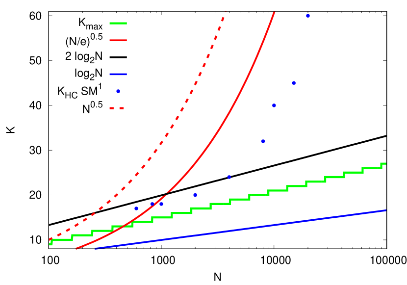
Figure 1.1: Hidden clique sizes $K_{HC}$ of interest in $G(N,p=0.5)$ lie between the $K_{\text{max}}$ staircase and the proven or experimentally observed lower limits that can be found with spectral methods (dashed red line) or message-passing techniques (solid red line). Sizes of the smallest hidden cliques identified by a simple greedy search from all initial sites, stopping as soon as evidence for the hidden clique is found, are shown with blue dots and lie well below both limits.

The simplest problems in combinatorial optimization are proving explicitly some property of a random graph, or proving that the property doesn’t hold in that graph. An example would be testing if the maximum size of a clique, or completely connected cluster of sites, of size $K$ exists in an Erdős-Rényi graph $G(N,p=0.5)$ of size $N$, with half of the bonds, selected at random, the rest absent. This is a stylization of a common question data scientists might ask of the social networks in tracking interaction on today’s network, where such graphs may describe populations of billions, and the bonds might be demonstrated common interests or communication. We know what is possible by just calculating expectations. The largest cliques, of size $K_{\text{max}}$, that form naturally in this model will not exceed $2\log_{2}N$ in size, with finite-size corrections making the actual limiting size of such a MaxClique much less. Simple linear algorithms, with costs proportional to the number of bonds, thus $N^{2}$, fail to find solutions with clique size $K$ more than a few sites bigger than $\log_{2}N$. A staircase of steps at which increasingly larger maximum cliques are found thus bounds a hard phase in which large numbers of cliques with sizes greater than $\log_{2}N$ must exist, but cannot be found without introducing some more expensive nonlinear search, such as backtracking.

A popular extension of this problem is to add a hidden clique to the random graph which is larger than those which occur at random. Since this clique is unique, it should be easier to find, but the best methods proven to work with quasi-linear cost (but large prefactors) can only find hidden cliques of size greater than $\sqrt{N/e}$. So an easy region for this related problem exists when the hidden clique is bigger than this line. The resulting phase diagram is shown in Fig. 1.1 [16].

Some recent work has returned to the original intuition of EA that correlations of activity between identical replicas of random, symmetry-less systems were an indication of ordering that might serve in place of a traditional order parameter. Consider simulating the evolution of multiple copies of a random system at steadily lowered temperatures, or at a number of different temperatures, and passing information about improved solutions between the different replicas, a methodology called parallel tempering in physics [17]. This has proved capable of finding hidden cliques in very large graphs when the hidden clique barely exceeds the size of naturally occurring cliques [18], as well as to find maximum independent sets very efficiently [19]. Annealing multiple replicas in this way has the disadvantage that it cannot be proven to have only polynomial cost (in the size of the problem) asymptotically, although experience and empirical knowledge of the problem may allow tuning the method for affordable costs on large practical problems. It may also provide a path to overcoming the confusion that impedes the search for optimal configurations in combinatorial problems where many suboptimal configurations overlap and confuse any local search, such as coloring or maximum clique [16].

The extra search power that parallel tempering seems to provide suggests that there may be other ways to exploit the original insight of Edwards and Anderson, that ordering in random systems might show up as a correlation between behavior observed in multiple copies or regions of a complex system. Replica symmetry breaking implies ordering which may take on a range of values, and study of the correlations seen in multiple replicas at low temperatures may add physical insight into such ordering. A further step could be to model systems which are basically similar but subject to weak local environmental corrections with a set of replicas, each slightly different. The objective would be to identify from the differences between solutions in each replica a functional variation of the response of ordering to the different local influences. Such local variations are typical of much of the vast amounts of social data available for study in today’s highly instrumented world. This is just one more possible, but as yet unrealized, impact of spin glasses on applied mathematics and statistics.

The original SK Ising model with Gaussian-distributed interactions is only one of the situations which has stimulated further exploration to tease out the lowest energy ground states. Different ways of combining different tools of optimization have proved valuable in this and different lessons emerge, as covered in the further sections of this chapter.

1.2 Focusing on Ground States

Consider the spin-glass (SG) model in zero field with Hamiltonian [2]

$${\cal H}=-\sum_{\langle i,j\rangle}J_{ij}s_{i}s_{j}.$$ (1.2)

We focus on Ising spins $s_{i}=\pm 1$ placed on the vertices of a graph, but other symmetries of the order parameter have been considered. The Ising symmetry has the advantage that the related statistical physics problems are combinatorial. The sum $\langle i,j\rangle$ runs over all edges of the graph. For the Edwards-Anderson (EA) model the graph is a hyper-cubic lattice in $d$ dimensions, but also other graph structures like the fully connected Sherrington-Kirkpatrick model corresponding to the $d\to\infty$ limit of (1.2) have been studied. As discussed in Chapter 1, the physics of this mean-field problem is well understood, in many aspects since the 1980s. The situation in low dimensions is less clear and so much of the work in recent decades has focused on studying the problem in 2, 3 and 4 dimensions with numerical methods.

Next to Monte Carlo simulations used to study the vicinity of the spin-glass transition and the behavior in the ordered phase (see Chapter 5), much work has been invested in studying ground states and low-lying excitations above them in order to gauge the low-temperature behavior. Alternative theories for the nature of the spin-glass phase make contrasting predictions about the energetic and geometric properties of such excitations. Based on generalizations of Peierls’ argument for the stability of the ferromagnetic phase, researchers have argued that excitations with energies diverging with length will lead to spin-glass phases that are stable against thermal fluctuations, such that one of the prime goals of studying ground states for spin-glass systems is to understand the nature of the prevalent low-energy excitations and how their sizes and energies are related.

The search for ground states for spin glasses with discrete symmetry amounts to a combinatorial optimization problem as there is a countable number of candidate solutions [20]. Such problems can hence be solved by a brute-force enumeration of all configurations, with an effort that grows exponentially with the number of spins. As discussed in section 1.3, a clever organization of this enumeration can lead to massive gains in efficiency of this process, but will not alter the overall exponential scaling of the process. This corresponds to the fact that the problem in $d\geq 3$ is known to be NP hard [21]. In some special cases, however, the ground-state problem can be mapped onto auxiliary optimization problems that permit solutions in polynomial time. This will be explained in section 1.4. Beyond the ground states of spin glasses, many optimization problems have caught the attention of physicists [22, 23]. An example for a recently studied model is the assignment problem, which is discussed in section 1.5.

1.3 Exact Algorithms for hard problems

Here, exact and general algorithms for finding ground states (GSs) for Ising SGs are considered, although the presented methods are very general. As an extension of Eq. (1.2), here also an interaction with local fields $h_{i}$ is included. For most studied systems no local field is present, but for some of the algorithms presented below, such a term might arise for sub-problems to be solved. In this case, the energy of a SG is given by the Hamiltonian

$${\cal H}(s)=-\sum_{i<j}J_{ij}s_{i}s_{j}\,-\sum_{i}h_{i}s_{i}\,,$$ (1.3)

where $s=(s_{1},\ldots,s_{N})$ is a configuration and the bonds $J_{ij}$, corresponding to the edges of the graph, are quenched random variables. The sum runs here, in the most general case, over all pairs of spins. Thus, if all bonds are nonzero, the system is of mean-field type. For finite-dimensional lattices, most bonds are zero, suitably selected. The nonzero bonds are typically drawn from a Gaussian or a bimodal $J_{ij}=\pm 1$ distribution.

Here, three types of algorithms are presented, which have frequently been used to calculate exact GSs for three-dimensional SGs. First, the branch-and-bound method is explained, which is based on enumerating many states in a sophisticated way. Next, the linear programming approach is outlined, which is based on rewriting the Hamiltonian as a linear function, relaxing the condition $s_{i}=\pm 1$, plus adding additional constraints, called cutting planes or cuts. Finally, the combination of both approaches, the branch-and-cut algorithm is presented, which yields the currently fastest exact method to obtain spin-glass ground states.

1.3.1 Branch-and-bound

The basic idea of the branch-and-bound approach [24] to find the minima of Eq. (1.3) is to represent all spin configurations as a binary tree, where at each node the configuration space is, for a node-dependent selected spin $i_{0}$, subdivided into the configurations with $s_{i_{0}}=+1$ and those with $s_{i_{0}}=-1$, respectively. The spin configurations are given by the $2^{N}$ leafs of this tree. The simplest approach to the GS problem would be to obtain all configurations by enumeration, and simply pick those with the minimum energy, yielding an $O(2^{N})$ running time.

This running time can be improved, although still being exponential in the worst case, by omitting parts of this tree via considering bounds on the achievable energies in sub-trees [25]. Here we present the refined algorithm described in Ref. [26]. The branching is performed always on the last spin of the sub-problem, i.e., it starts with spin $N$. The energies for the sub problems with $s_{N}=+1$ and $s_{N}=-1$ can be written using Eq. (1.3) for $\overline{s}=(s_{1},\ldots,s_{N-1})$ as follows:

$${\cal H}^{+}(\overline{s}) = -{\sum_{i<j}}^{\prime}J_{ij}s_{i}s_{j}-{\sum_{i}}^{\prime}h_{i}s_{i}-{\sum_{i}}^{\prime}J_{iN}s_{i}-h_{N}\;,$$ (1.4)

$${\cal H}^{-}(\overline{s}) = -{\sum_{i<j}}^{\prime}J_{ij}s_{i}s_{j}-{\sum_{i}}^{\prime}h_{i}s_{i}+{\sum_{i}}^{\prime}J_{iN}s_{i}+h_{N}\;,$$ (1.5)

where the sums $\sum^{\prime}$ run from $1$ to $N-1$. If one defines

$${\cal H}^{*}_{N-1}=\min_{s_{1},\ldots,s_{N-1}}-{\sum_{i<j}}^{\prime}J_{ij}s_{i}s_{j}\;,$$ (1.6)

one obtains, using the relation $\min_{s}(f_{1}(s)+f_{2}(s))\geq\min_{s}f_{1}(s)+\min_{s}f_{2}(s)$, the bounds

$${\cal H}^{+}(\overline{s}) \geq {\cal H}^{*}+\min_{s_{1},\ldots,s_{N-1}}{\sum_{i}}^{\prime}(-h_{i}-J_{in})s_{i}-h_{n}\;,$$ (1.7)

$${\cal H}^{-}(\overline{s}) \geq {\cal H}^{*}+\min_{s_{1},\ldots,s_{N-1}}-{\sum_{i}}^{\prime}(-h_{i}+J_{in})s_{i}+h_{n}\;.$$ (1.8)

These bounds are available because the minima ${\cal H}^{*}_{N-1}$, ${\cal H}^{*}_{N-2},\ldots$ can be obtained recursively while the branching tree is built. Furthermore, the minimum of a linear function $\sum_{s}\sum_{i}a_{i}s_{i}$, here $a_{i}=-h_{i}-J_{in}$ or $a_{i}=-h_{i}+J_{in}$, respectively, is simply given by $-\sum_{i}|a_{i}|$. Thus, as a first way to restrict the size of the branching tree, if one or two of the branches exhibit bounds above a known threshold, the corresponding branches can be omitted. Such thresholds may come from low lying configurations found already in other branches or by heuristic algorithms, or simply given as part of the problem in case an enumeration of a specified range of low-lying configurations is sought.

A second type of bound [26] works as follows. Using $d(\overline{s})=-2{\sum_{i}}^{\prime}J_{iN}s_{i}-2h_{N}$ one can rewrite Eqs. (1.4) and (1.5) as ${\cal H}^{+}(\overline{s})={\cal H}^{-}(\overline{s})+2d(\overline{s})$. Therefore, we obtain the implications

$$\max_{s_{1},\ldots,s_{N-1}}d(\overline{s})=2\sum_{i}|J_{iN}|-2h_{N}\leq 0 \,\Longrightarrow\, {\cal H}^{+}(\overline{s})\geq{\cal H}^{-}(\overline{s})\;,$$

$$\min_{s_{1},\ldots,s_{N-1}}d(\overline{s})=-2\sum_{i}|J_{iN}|-2h_{N}\geq 0 \,\Longrightarrow\, {\cal H}^{+}(\overline{s})\leq{\cal H}^{-}(\overline{s})\;.$$

These bounds are easy to calculate and allow sometimes for omitting one of the two branches, before any branch has to be evaluated.

Such branch-and-bound algorithms have been used, e.g., to analyze the low-temperature landscape [27, 28, 29, 30] of SGs. More broadly, in the field of statistical mechanics of optimization problems [22, 23], the branch-and-bound approach has been applied to other problems like the satisfiability problem [31] or the vertex-cover problem [32]. For the latter one, a branch-and-bound approach was used, where the variable to branch on was not selected in a given order but determined by a local heuristics for further reduction of the branching tree. For simple variants of these algorithms, it has also been possible to calculate analytically the typical running time for ensembles of random problems, which exhibit transitions between typically polynomial and typically exponential behavior [33, 34].

1.3.2 Linear programming and cutting planes

A different approach works by translating the quadratic Hamiltonian into a linear problem. For convenience, here we consider the form of Eq. (1.2) Note that the field term present in Eq. (1.3) can be written as quadratic term by introducing a “ghost spin” $s_{0}=1$ matching the given equation.

We describe the system by a graph $G=(V,E)$ where $V$ denotes the set of sites where the spins are located and $E$ the set of edges $\{i,j\}$ between the interacting sites. For any set $V^{\prime}\subset V$ in $G$ the cut $\delta(V^{\prime})\subset E$ denotes the set of edges where one endpoint is in $V^{\prime}$ and the other is not, i.e., those connecting the two sets $V^{\prime}$ and $V\setminus V^{\prime}$. For each configuration, the spins can be partitioned into two sets $V^{+}=\{i|s_{i}=+1\}$ of “up” spins and $V^{+}=\{i|s_{i}=-1\}=V\setminus V^{+}$ of “down” spins. If two spins $s_{i}$ and $s_{j}$ are oriented identically, they contribute the energy $-J_{ij}=+0-J_{ij}$, while they contribute the energy $J_{ij}=2J_{ij}-J_{ij}$ if they are oriented differently. Thus, using the cut, we can write

$${\cal H}(s)=2\sum_{\{i,j\}\in\delta(V^{+})}J_{ij}-\sum_{ij}J_{ij}\,.$$ (1.9)

By introducing $c_{ij}=-J_{ij}$, $S=\sum_{ij}J_{ij}$ and variables $x_{ij}=1$ if $\{i,j\}\in\delta(V^{+})$ and $x_{ij}=0$ else, this reads

$${\cal H}(x)=-2\sum_{i,j}c_{ij}x_{ij}-S\,,$$ (1.10)

where $\sum_{i,j}c_{ij}x_{ij}$ is called the weight of the cut represented by $x$. Therefore, since $S$ is only a constant, finding the minimum energy of Eq. (1.2) corresponds to finding the maximum cut in a graph with edge weights $c_{ij}$. Note that Eq. (1.10) is a linear function with integer variables, which means we have transformed the quadratic optimization problem into a linear one, but with additional constraints since $x$ must describe a cut. This problem is called integer linear program.

To include the constraints describing the cut, we note that for any cycle in the graph $G$ the cut must be crossed an even number of times. This can be conveniently described by linear inequalities [35] for the variables $x$ as follows: For any cycle $C\subset E$, i.e., a path which starts and ends at the same vertex, and any odd cardinality subset $Q\subset C$,

$$\sum_{\{i,j\}\in Q}x_{ij}-\sum_{\{i,j\}\in C\setminus Q}x_{ij}\leq|Q|-1$$ (1.11)

must hold, which defines a cut comprehensively.

The basic idea of the cutting-plane approach is now to relax the variables $x_{ij}=0,1$ to $0\leq x_{ij}\leq 1$ and look for a maximum of Eq. (1.10) given the linear inequalities Eq. (1.11). The name cutting plane comes from the fact that all inequalities describe hyper-planes which cut off one part from the space of possible solutions. The resulting problem is called a linear program (LP). The good news is that LPs, i.e., with the relaxed variables, can be solved [36] in worst-case polynomial time in the problem size using the ellipsoid method. Still, in a practical context methods like the simplex approach [37] or the dual simplex approach, which exhibit no polynomial bound, perform much faster. Still, the bad news is that the number of inequalities is in principle exponentially large, which would yield an exponential running time right-on. Therefore, instead of adding all constraints immediately to the LP, one starts with no or few constraints and calculates a first solution. Since fewer constraints than necessary are contained in the relaxed problem, typically the obtained cut weight will be higher, i.e., an upper bound of the true maximum cut for the integer LP. Hence, the obtained solution will typically not correspond to a cut and not be pure integer-valued. Thus, there may be some of the exponentially many inequalities which are violated. The second basic idea of the cutting plane approach is to look specifically for violated inequalities, without searching all possible ones, and add the violated ones to a growing set of inequalities included in the LP. An exact polynomial algorithm to find violated inequalities is based on solving a series of shortest-path problems [35], which can be done in $O(N^{3})$. This is polynomial but rather slow. Fortunately, there exist, in particular for physical lattice structures, several heuristics which run in linear $O(N)$ time [38] and are most of the time sufficient to generate additional inequalities for violated conditions. If at some point no further violated inequalities are found and the solution is fully integer-valued, a true optimum has been found, and the algorithm stops. But if on the contrary some variables are still non-integer, one can resort to branching as explained in the next subsection.

Nevertheless, for some combinatorial problems it has been observed that a cutting plane approach alone may lead to a valid optimum solution of the integer problem. For example for vertex-cover problems on Erdős-Rényi random graphs a different kind of cycle inequalities has been considered [39]. When varying the average number $c$ of neighbor nodes in the graphs, a phase transition has been observed. In the thermodynamic limit $N\to\infty$, for small values $c<c^{*}=e\approx 2.71$, typically all instances can be solved completely in a polynomial running time, while for larger values of $c$ this is not possible. Interestingly, this easy-hard transition coincides with the critical connectivity where replica-symmetry breaking of the vertex-cover problem occurs [32]. At this point a complex structure of the solution space has been observed [40], where the so-called leaf-removal core [41] starts to percolate.

Finally, note that there is a set of cutting planes, so called Gomory cuts [42], which can be constructed generally for all relaxed linear problems. They are based on identifying violated inequalities directly from a given non-integer solution, actually in the so-called tableau [36] used by the simplex algorithm to solve the LP. It is proven that this, possibly exponentially large, set of inequalities is complete, i.e. any integer programming problem can be solved in principle by generating just these cutting planes. Still, in practice, any finite numerical accuracy leads to convergence problems, such that this and many other cutting-plane approaches turned out to be actually efficient in combination with branching, as explained next.

1.3.3 Branch-and-cut

If for a relaxed linear system describing maximum cuts the solution is still non-integer, one considers for some variable $x_{ij}\neq 0,1$ both possibilities $x_{ij}=0$ and $x_{ij}=1$ and solves the corresponding sub-problems recursively. This means one branches. The combination of these approaches is therefore called branch-and-cut [43, 38]. Note that here several other bounds, in addition to those mentioned above, can be used. This can be lower bounds obtained from the cut weight of any valid cut $x^{*}$ or upper bounds obtained from suitable relaxations like the LP.

Currently, the branch-and-cut approach can be considered as the most powerful exact algorithm to obtain GSs for hard SG instances. A publicly accessible implementation of a branch-and-cut algorithm is the spin-glass server [44] hosted by the University of Bonn. The server was originally implemented at the University of Cologne by several members and collaborators of the research groups of F. Liers and M. Jünger. At the server, you can submit SG instances as a file and, if the system is not too large, a corresponding GS will be returned.

Branch-and-cut approaches have been applied to finite-dimensional SGs in several occasions. To our knowledge the largest three-dimensional instances were $N=12^{3}$ as considered in a study of low-lying excitations [45].

The approach has also been applied for a mean-field random-bond Ising model, which is a generalization of the standard SG with a variable fraction of negative bond as controlled by a non-zero mean of the bond values. Here, a phase transition of the typical branch-and-cut running time, as measured by the number of LPs solved, between an easy and a hard phase has been observed near the transition between ferromagnetic and SG behavior [46].

1.4 Ground states in two dimensions

We now turn to the case of ground-state problems permitting a polynomial-time solution. For the EA model of Eq. (1.2) this is the case in dimensions $d<3$. Since the 1d problem is rather trivial, the much more interesting case of this type is the EA model in two dimensions.

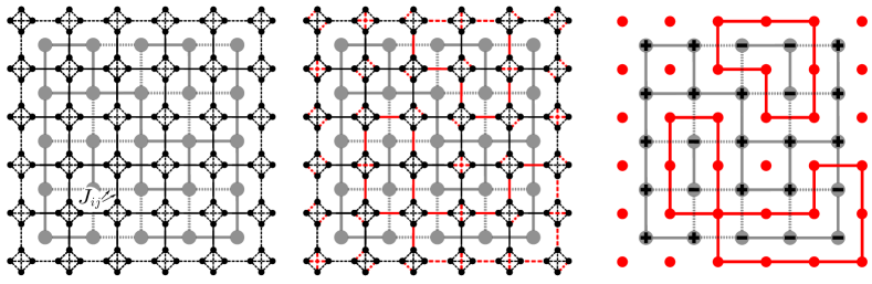
Figure 1.2: Mapping of the Ising ground-state problem to a matching problem on an auxiliary graph with Kasteleyn cities. Left: expansion of the Ising lattice, replacing each vertex by a complete graph $K_{4}$. Edge weights in the $K_{4}$ subgraphs are set to 0, the remaining weights are $J_{ij}$. Middle: A minimum-weight perfect matching on the auxiliary graph. Right: Back-transformation from the decorated graph to the original lattice. The matching then results in a set of closed loops separating up from down spins.

A relevant mapping of the EA ground state to a minimum-weight perfect matching (MWPM) problem on an auxiliary graph was first proposed in Ref. [47]. It is based on the observation that frustrated plaquettes [48], i.e., elementary lattice faces including an odd number of antiferromagntic couplings, must have an odd number of broken bonds with $J_{ij}s_{i}s_{j}<0$, while non-frustrated plaquettes have an even number of broken bonds. Hence a spin configuration can be depicted as a configuration of defect lines of broken bonds that start and end at frustrated plaquettes. A ground state configuration is then a perfect pairing (matching) of frustrated plaquettes through defect lines of minimum total weight. MWPM can be solved in polynomial time based on the blossom algorithm [49] and its variants [50]. However, this approach is still not ideal as it operates on the complete graph of the $F$ frustrated plaquettes with $F(F-1)$ edges, and the edge weights need to be computed in a preparatory step using a suitable approach such as Dijkstra’s algorithm [51] before attacking the matching problem. This approach allows one to study systems of a typical maximum linear size of $L\approx 500$ [52].

As was shown more recently [53, 54], an alternative mapping is significantly more efficient as it operates on a sparse graph with similar connectivity as the original lattice. It relies on an auxiliary graph that replaces each vertex of the lattice by a complete graph $K_{4}$ of four nodes, also known as Kasteleyn city. Edge weights are set to $J_{ij}$ for the original edges and to zero for the internal $K_{4}$ bonds. The solution of a matching problem on this graph then corresponds to a set of closed loops on the original lattice, separating domains of opposite spin orientations, cf. the illustration in Fig. 1.2. The configuration of minimum weight corresponds to a ground state of the spin-glass sample. Due to the sparsity of the auxiliary graph, significantly larger systems can be studied with this method as compared to the one proposed in [47], and calculations for square lattices up to $L=10\,000$ have been reported in Ref. [55].

A widely applied method for studying the excitations out of the ground states that take a central role in the theory of the spin-glass phase, consists of systematic modifications of boundary conditions (BCs). It is argued that the defect energy connected to a change from periodic to antiperiodic BCs in one direction,

$$E_{\mathrm{def}}=|E_{\mathrm{P}}-E_{\mathrm{AP}}|,$$ (1.12)

can act as a proxy for a typical low-energy excitation of the system [56]. Here, $E_{\mathrm{P}}$ and $E_{\mathrm{AP}}$ refers to the ground-state energy for periodic and antiperiodic BCs, respectively. One expects that $E_{\mathrm{def}}$ scales as [57, 58],

$$E_{\mathrm{def}}\sim L^{\theta}$$ (1.13)

with the spin-stiffness exponent $\theta$, where $\theta>0$ should indicate the stability of the spin-glass phase at non-zero temperatures, while for $\theta<0$ the transition temperature $T_{\mathrm{SG}}=0$ and $\theta=-1/\nu$ governs the divergence of the spin-glass correlation length as $T\to T_{\mathrm{SG}}$ [59]. For Gaussian exchange couplings $J_{ij}$ one finds a stiffness exponent $\theta\approx-0.3$ [52], with the most accurate estimate being [55],

$$\theta=-0.2793(3).$$ (1.14)

This is illustrated in Fig. 1.3(a) showing the scaling of defect energies over a wide range of system sizes. The change of boundary conditions induces a domain-wall defect that spans the system; a typical configuration of the overlap between the ground states for periodic and antiperiodic BCs is shown in the left panel of Fig. 1.4. The boundary of the flipped domain is a fractal curve, and the domain-wall length is hence expected to show fractal scaling of the form

$$\langle\ell\rangle_{J}=A_{\ell}L^{d_{\mathrm{f}}}.$$ (1.15)

As is illustrated in Fig. 1.3(b), this is indeed borne out in the data to high accuracy, and the fractal dimension is estimated as $d_{\mathrm{f}}=1.27319(9)$.

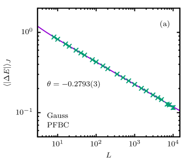
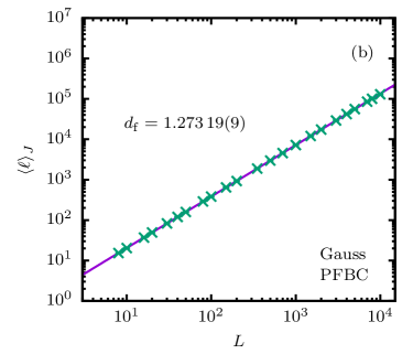
Figure 1.3: (a) Scaling of defect energies $E_{\mathrm{def}}$ for the Gaussian EA model on the square lattice with periodic boundaries in $x$ direction and free boundaries in $y$ direction. The line shows a fit of the data to the functional form $E_{\mathrm{def}}=A_{\theta}L^{\theta}+C_{\theta}/L^{2}$ [55]. (b) Scaling of the domain-wall length between periodic and antiperiodic BCs. The line corresponds to a fit of the functional form (1.15) to the data.

For technical reasons the matching approach can only handle samples on planar graphs, i.e., lattices with periodic boundary conditions in at most one direction [47]. More precisely, runs for systems with fully periodic boundaries yield the same result for periodic and for antiperiodic BCs in each of the two directions, such that the configuration returned is a ground state for one out of four possible BCs. As pointed out in Ref. [53], the approach hence effectively optimizes over BCs as well as spin variables. To circumvent this problem and allow treatment of systems with fully periodic BCs with the resulting smaller scaling corrections, one may use a windowing technique as illustrated in the right panel of Fig. 1.4: since MWPM can be used to find exact ground states for planar graphs, in order to treat a periodic $L\times L$ system one applies it to a square subset of edge length $L-2$ (“window”) while keeping the relative orientation of the outside spins fixed. Randomly displacing the window location over the (periodic) lattice, repeated applications of the window optimizations lead to a quick convergence of the result. This prescription results in a stochastic algorithm, whose success probability can be arbitrarily improved by using $m$ independent runs,

$$P_{s}(\{J_{ij}\})=1-[1-P_{n}(\{J_{ij}\})]^{m}.$$ (1.16)

Numerically, one finds that the number of required repetitions for a given success probability is independent of system size, such that the computational complexity of the algorithm remains the same as that of the MWPM approach for planar graphs, which scales as $L^{\kappa}$ with $\kappa\approx 2.2$ [55] for the Blossom V algorithm [50].

     

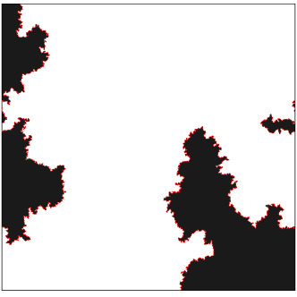
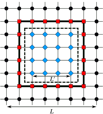
Figure 1.4: Left: The domain wall separating regions of equal and opposite ground-state configurations for a specific disorder sample considered with periodic and with antiperiodic boundaries. Right: Setup used for the windowing technique to compute ground states for samples with fully periodic boundary conditions.

The system with bimodal couplings can also be studied with matching techniques. Here, one finds no asymptotic decay of $E_{\mathrm{def}}$, but a convergence to a positive limiting value as $L\to\infty$ [52]. While this was initially taken as evidence for a lower-critical dimension $d_{l}=2$, it was later on realized that it is rather a signature of an additional zero-temperature renormalization-group fixed point that is not relevant for the physics at non-zero temperatures [60] and, instead, there is evidence for $d_{l}=2.5$ [61, 62]. A signature of this system is the extensive degeneracy of the ground state, leading to a finite ground-state entropy. This creates a difficulty for the matching approach as it does not pick the individual ground states with equal probabilities. In its simplest form, it is deterministic and will hence always return the same ground state. Some simple randomizations through changing the order of considering bonds or adding some noise onto the couplings improve on this, but still lead to biased sampling methods [55]. Unbiased sampling can be achieved via a suitably constructed Monte Carlo sampling technique in the ground-state manifold, thus allowing for estimates of the domain-wall fractal dimensions and related quantities [55].

Matching techniques can also be used to sample other excitations than the domain-wall perturbations induced by a change of boundary conditions. Different types of droplet-shaped excitations can be studied by fixing the relative orientation of spins through “hard” bonds [63, 64]. Also, while matching is the most widely used technique for this problem, an alternative approach based on a calculation of the partition function through the use of Pfaffians allows to also study finite-temperature properties exactly and in polynomial time [65, 66, 67]. Recently, such methods have been extended to also enable the study of correlation functions and further related properties [68, 69, 70].

1.5 The assignment problem

In this section we will discuss some new results in the assignment problem. In order to define the question in its simplest version we have to consider a square matrix of size $n$, $W:=\{w_{ij}\}_{i,j=1}^{n}$, with real entries. For each permutation $\pi$ in the symmetric group ${\mathcal{S}}_{n}$ consider the matrix $\Pi:=\{\pi_{ij}\}_{i,j=1}^{n}$ with entries zero or one, such that

$$\pi_{ij}=\delta_{j,\pi(i)}=\begin{cases}1&\hbox{\rm if\, }\pi(i)=j\\ 0&\hbox{\rm elsewhere}\end{cases}$$ (1.17)

and ask for a permutation of the columns of $W$ in order to get a minimum of the trace, that is of the Hamiltonian

$${\mathcal{H}}(\Pi,W):=\operatorname{tr}\left(W^{T}\cdot\Pi\right)=\sum_{i,j=1}^{n}w_{ij}\pi_{ij}=\sum_{i,j=1}^{n}w_{ij}\delta_{j,\pi(i)}=\sum_{i=1}^{n}w_{i,\pi(i)}\,.$$ (1.18)

Without loss of generality we can take the entries of $W$ to be nonnegative: $w_{ij}\geq 0$. Indeed, in combinatorial optimization they are usually referred to as costs. In different words, this is the classical matching problem on the bipartite complete graph ${\mathcal{K}}_{n,n}$. The solution of the problem is a permutation $\pi^{*}$, with corresponding matrix $\Pi^{*}(W)$ , that realizes the minimum cost and brings to the determination of

$${\mathcal{H}}^{*}(W):=\min_{\pi\in{\mathcal{S}}_{n}}{\mathcal{H}}(\Pi,W)={\mathcal{H}}\left(\Pi^{*}(W),W\right)$$ (1.19)

the optimal value of the total cost. The optimal solution can be seen as the ground state of the Hamiltonian of a disordered system defined by the cost-matrix $W$, an analogy which can be made useful, for example, by simulated annealing [7].

The introduction of a probability on the space of the possible costs allows the investigation of the properties of the typical solutions and the artillery from statistical physics shows its whole power [71, 22, 23]. In their seminal works Mézard and Parisi  [72, 73, 74] (but see also [75]) could solve, by using the replica trick, the matching, the assignment and the Travelling Salesman Problem in the case in which the entries $w_{ij}$ are independent random variables, equally distributed, with a probability distribution density of the form

$$\rho(w)=w^{r}\sum_{k=0}^{\infty}\eta_{k}w^{k}$$ (1.20)

with $\eta_{0}\neq 0$. More precisely, in the asymptotic limit of an infinitely large size $n$, replica symmetry is not broken, and the optimal solution is determined by the application of the saddle-point method as the solution of an integral equation in which only the parameter $r$ enters. In particular

$$E_{n}:=\mathbb{E}\left[{\mathcal{H}}^{*}(W)\right]\sim\,n^{1-\frac{1}{r+1}}\,,$$ (1.21)

where the expectation value is taken on the possible weights and with $\sim$ we indicate that both sides of the relation scale with large $n$ in the same way so that their ratio converges in the limit of an infinite number of points. For a recent work in which the first finite-size corrections are reconsidered after [76, 77] and the extension to non-integer value of the parameter $r$ see [78].

A new class of problems arises when the vertices of the graph ${\mathcal{K}}_{n,n}$ are identified with points in $\Omega\subset{\mathbb{R}}^{d}$ seen as a subset of a Euclidean space. We thus have two sets of points of cardinality $n$: we denote them as the red points $\mathcal{R}$, respectively blue points $\mathcal{B}$, with positions $x_{i}\in{\mathbb{R}}^{d}$, respectively $y_{i}\in{\mathbb{R}}^{d}$, with $i\in\{1,\dots,n\}=[n]$. Then the cost of the assignment of the $i$-th red point with the $j$-th blue point is assumed to be a function of the Euclidean distance between the two points $|x_{i}-y_{j}|$. We shall restrict to the cases

$$w_{ij}=f(|x_{i}-y_{j}|)=|x_{i}-y_{j}|^{p}$$ (1.22)

parametrized by the real number $p\in{\mathcal{R}}$. Let us introduce the empirical probability measures associated to the two sets of points

$$\rho_{\mathcal{R}}(x)=\frac{1}{n}\sum_{i=1}^{n}\delta(x-x_{i})\,;\qquad\rho_{\mathcal{B}}(y)=\frac{1}{n}\sum_{i=1}^{n}\delta(y-y_{j})$$ (1.23)

and look, for $p\geq 1$, at the $p$-th Wasserstein (elsewhere associated to the names of Kantorovich and Rubinstein) distance of two probability measures, that is at the variational problem

$$W_{p}(\rho_{1},\rho_{2}):=\left(\inf_{\gamma\in\Gamma(\rho_{1},\rho_{2})}\int dx\,dy\,\gamma(x,y)\,|x-y|^{p}\right)^{\frac{1}{p}}\,,$$ (1.24)

where $\Gamma(\rho_{1},\rho_{2})$ is the set of measures on $\Omega\times\Omega$ with marginals $\rho_{1}$ and $\rho_{2}$. This is nothing but the optimal transport (or Monge-Kantorovich) problem of a unit mass distributed according to $\rho_{1}$ to a distribution $\rho_{2}$ [79, 80]. A function $\gamma(x,y)$ defines a transportation plan, indeed, the marginality conditions

$$\int dx\,\gamma(x,y)=\rho_{2}(y)\,;\qquad\int dy\,\gamma(x,y)=\rho_{1}(x)$$ (1.25)

constraining the mass moved into the point $y$ and from the point $x$ are what is required. In the case of the two empirical probability measures the possible transportation plans reduce to the set of permutations and therefore their Wasserstein distance is simply related to the optimal cost [81]

$${\mathcal{H}}^{*}(W)=n\,W_{p}^{p}(\rho_{\mathcal{R}},\rho_{\mathcal{B}}).$$ (1.26)

A random matrix, whose elements depend on the Euclidean distance between points randomly distributed in space is called Euclidean. The spectra of Euclidean random matrices have been studied in [82].

In order to fix the ideas, let us consider the case in which $\Omega=[0,1]^{d}$, periodic boundary conditions are chosen, so that we are really on a torus of unit volume and the positions of red and blue points are taken at random with flat probability. A natural length-scale is therefore $n^{-\frac{1}{d}}$ and one can simply assume that for each red point there is at least a blue point to match in a ball of radius of order $n^{-\frac{1}{d}}$, so that we can guess that

$$E_{n}\sim n^{1-\frac{p}{d}}\,.$$ (1.27)

But it is well known [83] that this can be true only in $d\geq 2$. It was proven that in $d=2$

$$E_{n}\sim n\,\left(\frac{\log n}{n}\right)^{\frac{p}{2}}$$ (1.28)

a logarithmic violation appears. A much more detailed analysis is possible in $d=1$ [84] where an intriguing relation with Brownian processes is explored [85]. It is shown that, for a generic distribution probability $\rho$ with cumulative $\Phi$, the average total cost is

$$E_{n}=n^{1-\frac{p}{2}}\frac{2^{p}}{\sqrt{\pi}}\Gamma\left(\frac{p+1}{2}\right)\int_{0}^{1}dx\frac{[\Phi(x)(1-\Phi(x))]^{\frac{p}{2}}}{\rho^{p-1}(x)}+o(n^{-\frac{p}{2}})$$ (1.29)

at least when the integral is convergent. Otherwise an anomalous scaling emerges [86]. In the case of open boundary conditions, with flat distribution, the average cost can be evaluated even for finite size by means of Selberg integrals [87]

$$E_{n}=n\,\frac{\Gamma\left(1+\frac{p}{2}\right)}{p+1}\frac{\Gamma(n+1)}{\Gamma\left(n+1+\frac{p}{2}\right)}\,.$$ (1.30)

Also the case $p\leqslant 0$ has been studied [88], where, instead, for flat distribution

$$\lim_{n\to\infty}\frac{E_{n}}{n}=\frac{1}{2^{p}}\,.$$ (1.31)

When $0<p<1$ the cost function becomes concave. In [89] it is argued that

$$E_{n}\sim\begin{cases}n^{1-p}&\hbox{\rm for\,}0<p<\frac{1}{2}\,,\\ \sqrt{n}\log n&\hbox{\rm for\,}p=\frac{1}{2}\,,\\ \sqrt{n}&\hbox{\rm for\,}\frac{1}{2}<p<1\,,\\ \end{cases}$$ (1.32)

so that a change in the phase diagram occurs at $p=\frac{1}{2}$.

An amusing exact result has been obtained for the flat distribution in $d=2$ for the particular value $p=2$, in [90, 91], that is

$$\lim_{n\to\infty}\frac{E_{n}}{\log n}=\frac{1}{2\pi}.$$ (1.33)

This has been rigorously proven in [92] (see also [93] for improvements). Let us follow the field theoretic approach introduced in [94] and let us introduce the vector transport field $\mu(x)$ which joins the red point in $x$ to the blue point in $y=x+\mu(x)$ and consider the Lagrangian

$${\mathcal{L}}[\mu,\phi]:=\frac{1}{2}\int\mu^{2}(x)\rho_{\mathcal{R}}(dx)+\int\left[\phi(x+\mu(x))\rho_{\mathcal{R}}(dx)-\phi(x)\rho_{\mathcal{B}}(dx)\right]$$ (1.34)

to be minimized, where the scalar field $\phi(x)$ is a Lagrangian multiplier which implements a matching between blue and red points. In the limit of a large number of points $n$, when the red and blue points are extracted with the same distribution $\rho$ so that $\delta\rho:=\rho_{\mathcal{R}}-\rho_{\mathcal{B}}$ and the optimal $\mu$ goes to zero and we expect a good approximation by using the only the quadratic terms in the Lagrangian, that is

$${\mathcal{L}}[\mu,\phi]:=\int\left[\frac{1}{2}\mu^{2}(x)+\mu(x)\cdot\nabla\phi(x)\rho(dx)\right]+\int\phi(x)\delta\rho(dx)\,,$$ (1.35)

which has Euler-Lagrangian equations

$$\mu=-\nabla\phi\,,\qquad\nabla\cdot[\rho\,\mu]=\delta\rho\,,$$ (1.36)

revealing a strict analogy with an electrostatic problem where $\mu$ plays the role of the electric field, $\phi$ is the scalar potential and indeed is the Lagrangian multiplier which implements the Gauss law, red and blue points have opposite unit charge, being null the total charge, while $\rho$ is the dielectric function of a linear dielectric medium. As a consequence

$$-\nabla\cdot[\rho\,\nabla\phi]=\rho$$ (1.37)

is solved by means of the classical Green’s function $G_{\rho}(x,y)$ of the operator $-\nabla\cdot[\rho\,\nabla\bullet]$, so that an explicit approximate solution at fixed disorder is given by

$$\mu(x)=\int\nabla_{x}G_{\rho}(x,y)\,\delta\rho(dy)\,.$$ (1.38)

After averaging over disorder, in the simple case of a flat measure (see [95] for non-constant case) we get

$$\lim_{n\to\infty}E_{n}(\Omega)=-2\operatorname{tr}\Delta^{-1}_{\Omega}\,,$$ (1.39)

where the Laplacian $\Delta_{\Omega}$ is defined on the domain $\Omega$. This formula is correct in $d=1$ but it simply provides a divergence on both sides for $d>1$. It is an ultraviolet divergence which has been introduced by the linearization in the infinite number of modes, but the approximation cannot be true at very short distances. In the exact non-linear theory higher modes are cut off and we expect that

$$E_{n}(\Omega)=2\int_{0^{+}}^{\infty}\frac{F\left(\frac{\lambda}{n}\right)}{\lambda}\,d\mathcal{N}_{\Omega}(\lambda)\,,$$ (1.40)

where $\mathcal{N}_{\Omega}(\lambda)$ is number of the eigenvalue less than $\lambda$ for the Laplace operator and the unknown function $F$ interpolates between 1 for $\lambda\lesssim n$ and 0 for $\lambda\gtrsim n$.

By the Weyl law [96] on the asymptotics of the eigenvalue counting function for the Laplace-Beltrami operator we know that, for a 2-$d$ manifold with unit volume (under Neumann boundary conditions which are appropriate for our problem)

$$\mathcal{N}_{\Omega}(\lambda)=\frac{1}{4\pi}\left(\lambda+\sqrt{\lambda}\,|\partial\Omega|\right)+o\left(\sqrt{\lambda}\right)\,.$$ (1.41)

In $d=2$ it is easy now to evaluate the leading logarithmic singularity in the number of points and in agreement with [97] we expect that

$$E_{n}(\Omega)=\frac{1}{2\pi}\log n+2c_{*}(n)+2c_{\Omega}+o(1)\,,$$ (1.42)

where $c_{*}(n)=O(\log n)$ is a universal function not depending on $\Omega$. As a further consequence,

$$\lim_{n\to\infty}\left[E_{n}(\Omega)-E_{n}(\Omega^{\prime})\right]=2\lim_{n\to\infty}\int_{0^{+}}^{\infty}\frac{F\left(\frac{\lambda}{n}\right)}{\lambda}\,\left[d\mathcal{N}_{\Omega}(\lambda)-d\mathcal{N}_{\Omega^{\prime}}(\lambda)\right]\,,$$ (1.43)

but the r.h.s. is convergent even in the absence of regularization thus

$$\lim_{n\to\infty}\left[E_{n}(\Omega)-E_{n}(\Omega^{\prime})\right]=2\int_{0^{+}}^{\infty}\frac{d\mathcal{N}_{\Omega}(\lambda)-d\mathcal{N}_{\Omega^{\prime}}(\lambda)}{\lambda}\,,$$ (1.44)

an expression that has been tested in [98] on various 2$d$ manifolds, by using both the Green’s function method as other classical tools as the Dedekind’s limit formulas, thus confirming the predictions of the field theoretic approach.

For a similar method applied to a more general context see [99, 100, 101].

Once more this relatively simple combinatorial optimization problem is revealing intriguing and fruitful connections with so many different research fields.

References

- [1] R. Brout, Statistical mechanical theory of a random ferromagnetic system, Phys. Rev. 115(4), 824, (1959).
- [2] S. F. Edwards and P. W. Anderson, Theory of spin glasses, J. Phys. F. 5, 965, (1975).
- [3] D. Sherrington and S. Kirkpatrick, Solvable model of a spin-glass, Phys. Rev. Lett. 35(26), 1792, (1975).
- [4] S. Kirkpatrick and D. Sherrington, Infinite-ranged models of spin-glasses, Phys. Rev. B. 17(11), 4384, (1978).
- [5] A. Crisanti and T. Rizzo, Analysis of the replica symmetry breaking solution of the Sherrington-Kirkpatrick model, Phys. Rev. E. 65(4), 046137, (2002).
- [6] S.-Y. Kim, S. J. Lee, and J. Lee, Ground-state energy and energy landscape of the Sherrington-Kirkpatrick spin glass, Phys. Rev. B. 76(18), 184412, (2007).
- [7] S. Kirkpatrick, C. D. Gelatt, and M. P. Vecchi, Optimization by simulated annealing, Science. 220(4598), 671–680, (1983). URL http://science.sciencemag.org/content/220/4598/671.long.
- [8] V. Černỳ, Thermodynamical approach to the traveling salesman problem: An efficient simulation algorithm, Journal of optimization theory and applications. 45(1), 41–51, (1985).
- [9] K. G. Wilson. Personal communication to Scott Kirkpatrick, (1990).
- [10] B. Selman. The next generation of automated reasoning methods, (2021). Slides of lecture CS6700 at Cornell University.
- [11] M. Mézard, G. Parisi, and R. Zecchina, Analytic and algorithmic solution of random satisfiability problems, Science. 297(5582), 812–815, (2002).
- [12] M. Mézard and G. Parisi, The cavity method at zero temperature, J. Stat. Phys. 111(1), 1–34, (2003).
- [13] F. Krzakała, A. Montanari, F. Ricci-Tersenghi, G. Semerjian, and L. Zdeborová, Gibbs states and the set of solutions of random constraint satisfaction problems, Proc. Natl. Acad. Sci. U.S.A. 104(25), 10318–10323, (2007).
- [14] L. Zdeborova, Statistical physics of hard optimization problems, Acta Physica Slovaca. 59, (2009).
- [15] D. Gamarnik, The overlap gap property: A topological barrier to optimizing over random structures, Proc. Natl. Acad. Sci. U.S.A. 118(41), e2108492118, (2021).
- [16] R. Marino and S. Kirkpatrick, Hard optimization problems have soft edges, arXiv:2209.04824. (2022).
- [17] K. Hukushima and K. Nemoto, Exchange Monte Carlo method and application to spin glass simulations, J. Phys. Soc. Jpn. 65(6), 1604–1608, (1996).
- [18] M. C. Angelini, Parallel tempering for the planted clique problem, J. Stat. Mech.: Theory Exp. 2018(7), 073404, (2018).
- [19] M. C. Angelini and F. Ricci-Tersenghi, Monte Carlo algorithms are very effective in finding the largest independent set in sparse random graphs, Phys. Rev. E. 100(1), 013302, (2019).
- [20] A. K. Hartmann and H. Rieger, Optimization Algorithms in Physics. (Wiley, Berlin, 2002).
- [21] F. Barahona, On the computational complexity of Ising spin glass models, J. Phys. A. 15, 3241, (1982). URL http://dx.doi.org/10.1088/0305-4470/15/10/028.
- [22] A. K. Hartmann and M. Weigt, Phase Transitions in Combinatorial Optimization Problems: Basics, Algorithms and Statistical Mechanics. (Wiley, 2006).
- [23] M. Mézard and A. Montanari, Information, physics, and computation. (Oxford University Press, 2009).
- [24] A. H. Land and A. G. Doig, An automatic method for solving discrete programming problems, Exonometrica. 28, 497, (1960).
- [25] S. Kobe and A. Hartwig, Exact ground state of finite amorphous Ising systems, Comp. Phys. Commun. 16(1), 1–4, (1978). ISSN 0010-4655. https://doi.org/10.1016/0010-4655(78)90102-9.
- [26] A. Hartwig, F. Daske, and S. Kobe, A recursive branch-and-bound algorithm for the exact ground state of Ising spin-glass models, Comp. Phys. Commun. 32(2), 133–138, (1984). ISSN 0010-4655. https://doi.org/10.1016/0010-4655(84)90066-3.
- [27] T. Klotz and S. Kobe, Geometry of ground-state clusters in the configuration space of finite 3d j spin glasses, J. Magn. Magn. Mat. 177-181, 1359–1360, (1998). ISSN 0304-8853. https://doi.org/10.1016/S0304-8853(96)00775-5. International Conference on Magnetism (Part II).
- [28] T. Klotz, S. Schubert, and K. H. Hoffmann, The state space of short-range Ising spin glasses: the density of states, Europ. Phys. J. B. 2(3), 313–317 (Apr, 1998). ISSN 1434-6036. 10.1007/s100510050254.
- [29] J. Krawczyk and S. Kobe, Low-temperature dynamics of spin glasses: walking in the energy landscape, Physica A. 315(1), 302–307, (2002). ISSN 0378-4371. https://doi.org/10.1016/S0378-4371(02)01227-X. Slow Dynamical Processes in Nature.
- [30] S. Schubert and K. H. Hoffmann, The structure of enumerated spin glass state spaces, Comp. Phys. Commun. 174(3), 191–197, (2006). ISSN 0010-4655. https://doi.org/10.1016/j.cpc.2004.02.019.
- [31] R. Monasson, R. Zecchina, S. Kirkpatrick, B. Selman, and L. Troyansky, Determining computational complexity from characteristic phase transitions, Nature. 400, 133, (1999).
- [32] M. Weigt and A. K. Hartmann, The number guards needed by a museum – a phase transition in vertex covering of random graphs, Phys. Rev. Lett. 84, 6118, (2000).
- [33] S. Cocco and R. Monasson, Trajectories in phase diagrams, growth processes, and computational complexity: How search algorithms solve the 3-satisfiability problem, Phys. Rev. Lett. 86, 1654, (2001).
- [34] M. Weigt and A. K. Hartmann, The typical-case complexity of a vertex-covering algorithm on finite-connectivity random graphs, Phys. Rev. Lett. 86, 1658, (2001).
- [35] F. Barahona and A. R. Mahjoub, On the cut polytope, Math. Program. 36(2), 157–173 (Jun, 1986). ISSN 1436-4646. 10.1007/BF02592023.
- [36] M. Padberg, Linear Programming and extensions. (Springer, Berlin, 1995).
- [37] G. B. Dantzig, Programming in a linear structure, Bull. Amer. Math. Soc. 54, 1074–1074, (1948).
- [38] F. Liers, M. Jünger, G. Reinelt, and G. Rinaldi. Computing exact ground states of hard Ising spin glass problems by Branch-and-cut. In eds. A. K. Hartmann and H. Rieger, New Optimization Algorithms in Physics, p. 47. Whiley-VCH, Weinheim, (2004).
- [39] T. Dewenter and A. K. Hartmann, Phase transition for cutting-plane approach to vertex-cover problem, Phys. Rev. E. 86, 041128, (2012). 10.1103/PhysRevE.86.041128.
- [40] W. Barthel and A. K. Hartmann, Clustering analysis of the ground-state structure of the vertex-cover problem, Phys. Rev. E. 70, 066120, (2004).
- [41] M. Bauer and O. Golinelli, Core percolation in random graphs: a critical phenomena analysis, Eur. Phys. J. B. 24, 339, (2001).
- [42] R. E. Gomory, Outline of an algorithm for integer solutions to linear programs, Bull. Am. Math. Soc. 64(5), 275–278, (1958).
- [43] F. Barahona, M. Grötschel, M. Jünger, and G. Reinelt, An application of combinatorial optimization to statistical physics and circuit layout design, Operations Research. 36(3), 493, (1988). ISSN 0030364X.
- [44] S. Mallach. Spin-glass Server. http://spinglass.uni-bonn.de/, (2022). Accessed: 2022-05-04.
- [45] M. Palassini, F. Liers, M. Jünger, and A. P. Young, Low-energy excitations in spin glasses from exact ground states, Phys. Rev. B. 68, 064413 (Aug, 2003). 10.1103/PhysRevB.68.064413.
- [46] F. Liers, M. Palassini, A. K. Hartmann, and M. Jünger, Ground state of the Bethe lattice spin glass and running time of an exact optimization algorithm, Phys. Rev. B. 68, 094406 (Sep, 2003). 10.1103/PhysRevB.68.094406.
- [47] I. Bieche, R. Maynard, R. Rammal, and J. P. Uhry, On the ground-states of the frustration model of a spin-glass by a matching method of graph-theory, J. Phys. A. 13, 2553, (1980). URL http://dx.doi.org/10.1088/0305-4470/13/8/005.
- [48] G. Toulouse, Theory of frustration effect in spin glasses 1, Commun. Phys. 2, 115, (1977). URL http://dx.doi.org/10.1142/9789812799371_0009.
- [49] J. Edmonds, J. Res. Natl. Bur. Stand. B. 69, 125, (1965).
- [50] V. Kolmogorov, Blossom V: a new implementation of a minimum cost perfect matching algorithm, Math. Prof. Comp. 1, 43, (2009). URL http://dx.doi.org/10.1007/s12532-009-0002-8.
- [51] A. Gibbons, Algorithmic Graph Theory. (Cambridge University Press, Cambridge, 1985).
- [52] A. K. Hartmann and A. P. Young, Lower critical dimension of Ising spin glasses, Phys. Rev. B. 64(18), 180404, (2001). URL http://dx.doi.org/10.1103/physrevb.64.180404.
- [53] C. K. Thomas and A. A. Middleton, Matching Kasteleyn cities for spin glass ground states, Phys. Rev. B. 76, 220406, (2007). URL http://dx.doi.org/10.1103/PhysRevB.76.220406.
- [54] G. Pardella and F. Liers, Exact ground states of large two-dimensional planar Ising spin glasses, Phys. Rev. E. 78, 056705, (2008). URL http://dx.doi.org/10.1103/PhysRevE.78.056705.
- [55] H. Khoshbakht and M. Weigel, Domain-wall excitations in the two-dimensional Ising spin glass, Phys. Rev. B. 97, 064410, (2018). URL http://arxiv.org/abs/1710.01670.
- [56] J. R. Banavar and M. Cieplak, Nature of ordering in spin-glasses, Phys. Rev. Lett. 48, 832, (1982).
- [57] A. J. Bray and M. A. Moore, Lower critical dimension of Ising spin glasses: a numerical study, J. Phys. C. 17, (1984).
- [58] W. L. McMillan, Scaling theory of Ising spin glasses, J. Phys. C. 17, 3179, (1984).
- [59] A. J. Bray and M. A. Moore. Scaling theory of the ordered phase of spin glasses. In eds. J. L. van Hemmen and I. Morgenstern, Heidelberg Colloquium on Glassy Dynamics, p. 121, Heidelberg, (1987). Springer.
- [60] T. Jörg and F. Krzakala, The nature of the different zero-temperature phases in discrete two-dimensional spin glasses: entropy, universality, chaos and cascades in the renormalization group flow, J. Stat. Mech.: Theory Exp. 2012(01), L01001, (2012). URL http://dx.doi.org/10.1088/1742-5468/2012/01/l01001.
- [61] S. Boettcher, Stiffness of the Edwards-Anderson model in all dimensions, Phys. Rev. Lett. 95, 197205, (2006).
- [62] A. Maiorano and G. Parisi, Support for the value 5/2 for the spin glass lower critical dimension at zero magnetic field, Proc. Natl. Acad. Sci. U.S.A. 115(20), 5129–5134, (2018).
- [63] A. K. Hartmann and M. A. Moore, Corrections to scaling are large for droplets in two-dimensional spin glasses, Phys. Rev. Lett. 90, 127201, (2003).
- [64] A. K. Hartmann, Droplets in the two-dimensional Ising spin glass, Phys. Rev. B. 77, 144418, (2008). URL http://dx.doi.org/10.1103/physrevb.77.144418.
- [65] J. A. Blackman and J. Poulter, Gauge-invariant method for the spin-glass model, Phys. Rev. B. 44, 4374–4386, (1991). URL http://dx.doi.org/10.1103/physrevb.44.4374.
- [66] L. Saul and M. Kardar, Exact integer algorithm for the two-dimensional Ising spin glass, Phys. Rev. E. 48(5), R3221, (1993). URL http://dx.doi.org/10.1103/PhysRevE.48.R3221.
- [67] A. Galluccio, M. Loebl, and J. Vondrák, New algorithm for the Ising problem: Partition function for finite lattice graphs, Phys. Rev. Lett. 84(26), 5924, (2000). URL http://dx.doi.org/10.1103/PhysRevLett.84.5924.
- [68] C. K. Thomas and A. A. Middleton, Exact algorithm for sampling the two-dimensional Ising spin glass, Phys. Rev. E. 80, 046708, (2009). URL http://dx.doi.org/10.1103/PhysRevE.80.046708.
- [69] C. K. Thomas, D. A. Huse, and A. A. Middleton, Zero- and low-temperature behavior of the two-dimensional Ising spin glass, Phys. Rev. Lett. 107, 047203, (2011). URL http://dx.doi.org/10.1103/physrevlett.107.047203.
- [70] C. K. Thomas and A. A. Middleton, Numerically exact correlations and sampling in the two-dimensional Ising spin glass, Phys. Rev. E. 87, 043303 (Apr, 2013). URL https://link.aps.org/doi/10.1103/PhysRevE.87.043303.
- [71] M. Mézard, G. Parisi, and M. Virasoro, Spin glass theory and beyond: An Introduction to the Replica Method and Its Applications. vol. 9, (World Scientific Publishing Company, 1987).
- [72] M. Mézard and G. Parisi, Replicas and optimization, J. Phys. (Paris) - Lettres. 46(17), 771–778, (1985). ISSN 0302-072X. 10.1051/jphyslet:019850046017077100. URL http://www.edpsciences.org/10.1051/jphyslet:019850046017077100.
- [73] M. Mézard and G. Parisi, A replica analysis of the travelling salesman problem, J. Phys. (Paris). 47(1986), 1285–1296, (1986). URL http://jphys.journaldephysique.org/index.php?option=com{_}article{&}access=doi{&}doi=10.1051/jphys:019860047080128500.
- [74] M. Mézard and G. Parisi, Mean-field equations for the matching and the travelling salesman problems, Europhysics Letters. 2(12), 913–918, (1986).
- [75] H. Orland, Mean-field theory for optimization problems, Le J. Phys. (Paris) - Lettres. 46(17), 773–770, (1985). 10.1051/jphyslet:019850046017076300. URL https://jphyslet.journaldephysique.org/articles/jphyslet/abs/1985/17/jphyslet_1985__46_17_763_0/jphyslet_1985__46_17_763_0.html.
- [76] M. Mézard and G. Parisi, On the solution of the random link matching problems, J. Phys. (Paris). 48(9), 1451–1459, (1987). ISSN 0302-0738. 10.1051/jphys:019870048090145100. URL http://jphys.journaldephysique.org/index.php?option=com{_}article{&}access=doi{&}doi=10.1051/jphys:019870048090145100http://www.edpsciences.org/10.1051/jphys:019870048090145100.
- [77] G. Parisi and M. Ratiéville, On the finite size corrections to some random matching problems, Eur. Phys. J. B. 29(3), 457–468 (oct, 2002). ISSN 1434-6028. 10.1140/epjb/e2002-00326-3.
- [78] S. Caracciolo, M. P. D’Achille, E. M. Malatesta, and G. Sicuro, Finite size corrections in the random assignment problem, Phys. Rev. E. 95, 052129, (2017). 10.1103/PhysRevE.95.052129. URL https://journals-aps-org.pros.lib.unimi.it:2050/pre/abstract/10.1103/PhysRevE.95.052129.
- [79] C. Villani, Optimal transport: old and new. vol. 338, (Springer Science & Business Media, 2008).
- [80] L. Ambrosio, Mathematical Aspects of Evolving Interfaces, vol. 1812, Lecture Notes in Mathematics (Fondazione C.I.M.E., Firenze), chapter Lecture notes on optimal transport problems, pp. 1–52. Springer, Berlin, Heidelberg, (2003).
- [81] H. Brezis, Remarks on the Monge–Kantorovich problem in the discrete setting, Comptes Rendus Mathematique. 356(2), 207 – 213, (2018). ISSN 1631-073X. https://doi.org/10.1016/j.crma.2017.12.008. URL http://www.sciencedirect.com/science/article/pii/S1631073X1730328X.
- [82] M. Mézard, G. Parisi, and A. Zee, Spectra of Euclidean random matrices, Nuclear Physics B. 559(3), 689 – 701, (1999). ISSN 0550-3213. https://doi.org/10.1016/S0550-3213(99)00428-9. URL http://www.sciencedirect.com/science/article/pii/S0550321399004289.
- [83] M. Ajtai, J. Komlós, and G. Tusnády, On optimal Matchings, Combinatorica. 4(4), 259–264, (1984).
- [84] E. Boniolo, S. Caracciolo, and A. Sportiello, Correlation function for the Grid-Poisson Euclidean matching on a line and on a circle, J. Stat. Mech. 11, P11023, (2014). 10.1088/1742-5468/2014/11/P11023.
- [85] S. Caracciolo and G. Sicuro, On the one dimensional Euclidean matching problem: exact solutions, correlation functions and universality, Phys. Rev. E. 90, 042112, (2014). 10.1103/PhysRevE.90.042112. URL https://journals-aps-org.pros.lib.unimi.it/pre/abstract/10.1103/PhysRevE.90.042112.
- [86] S. Caracciolo, M. P. D’Achille, and G. Sicuro, Anomalous scaling of the optimal cost in the one-dimensional random assignment problem, J. Stat. Phys. 174(4), 846–864, (2019). 10.1007/s10955-018-2212-9. URL https://link.springer.com/article/10.1007%2Fs10955-018-2212-9.
- [87] S. Caracciolo, A. Di Gioacchino, E. M. Malatesta, and L. G. Molinari, Selberg integrals in 1D random Euclidean optimization problems, J. Stat. Mech. p. 063401, (2019). 10.1088/1742-5468/ab11d7. URL https://iopscience-iop-org.pros.lib.unimi.it:2050/article/10.1088/1742-5468/ab11d7/pdf.
- [88] S. Caracciolo, M. P. D’Achille, and G. Sicuro, Random Euclidean matching problems in one dimension, Phys. Rev. E. 96, 042102, (2017). 10.1103/PhysRevE.96.042102. URL https://journals-aps-org.pros.lib.unimi.it/pre/pdf/10.1103/PhysRevE.96.042102.
- [89] S. Caracciolo, M. P. D’Achille, V. Erba, and A. Sportiello, The Dyck bound in the concave 1-dimensional random assignment model, J. Phys. A: Math. Theor. 53(6), 064001 (25pp), (2020). 10.1088/1751-8121/ab4a34. URL https://doi.org/10.1088%2F1751-8121%2Fab4a34.
- [90] S. Caracciolo, C. Lucibello, G. Parisi, and G. Sicuro, Scaling hypothesis for the Euclidean bipartite matching problem, Phys. Rev. E. 90, 012118, (2014). 10.1103/PhysRevE.90.012118. URL https://journals-aps-org.pros.lib.unimi.it/pre/abstract/10.1103/PhysRevE.90.012118.
- [91] S. Caracciolo and G. Sicuro, Scaling hypothesis for the Euclidean bipartite matching problem. II. Correlation functions, Phys. Rev. E. 91, 062125, (2015). http://dx.doi.org/10.1103/PhysRevE.91.062125. URL https://journals-aps-org.pros.lib.unimi.it/pre/abstract/10.1103/PhysRevE.91.062125.
- [92] L. Ambrosio, F. Stra, and D. Trevisan, A PDE approach to a -dimensional matching problem, Probab. Theory Relat. Fields. 173, 433–477, (2019). 10.1007/s00440-018-0837-x. URL https://doi.org/10.1007/s00440-018-0837-x.
- [93] L. Ambrosio, F. Glaudo, and D. Trevisan, On the optimal map in the 2-dimensional random matching problem, Discrete Cont. Dyn. A. 39, 1078–0947, (2019). 10.3934/dcds.2019304. URL http://aimsciences.org//article/id/17beca52-6bdd-4a1a-a9c9-4b2145874254.
- [94] S. Caracciolo and G. Sicuro, Quadratic stochastic Euclidean bipartite matching problem, Phys. Rev. Lett. 115(23), 230601, (2015). http://dx.doi.org/10.1103/PhysRevLett.115.230601. URL http://journals.aps.org/prl/abstract/10.1103/PhysRevLett.115.230601.
- [95] D. Benedetto and E. Caglioti, Euclidean random matching in 2d for non-constant densities, J. Stat. Phys. 181, 854–869, (2020).
- [96] V. Ivrii, 100 years of Weyl’s law, Bull. Math. Sci. 6(3), 379–452, (2016). 10.1007/s13373-016-0089-y.
- [97] L. Ambrosio and F. Glaudo, Finer estimates on the 2-dimensional matching problem, J. Éc. Polytech. Math. 6, 737–765, (2019).
- [98] D. Benedetto, E. Caglioti, S. Caracciolo, M. P. D’Achille, G. Sicuro, and A. Sportiello, Random assignment problem on manifolds, J. Stat. Phys. 183, 34, (2021). 10.1007/s10955-021-02768-4. URL https://arxiv.org/abs/2008.01462.
- [99] P. Koehl, M. Delarue, and H. Orland, Statistical physics approach to the optimal transport problem, Phys. Rev. Lett. 123, 040603, (2019). 10.1103/PhysRevLett.123.040603. URL https://link.aps.org/doi/10.1103/PhysRevLett.123.040603.
- [100] P. Koehl and H. Orland, Fast computation of exact solutions of generic and degenerate assignment problems, Phys. Rev. E. 103, 042101, (2021). 10.1103/PhysRevE.103.042101. URL https://link.aps.org/doi/10.1103/PhysRevE.103.042101.
- [101] P. Koehl, M. Delarue, and H. Orland, Physics approach to the variable-mass optimal-transport problem, Phys. Rev. E. 103, 012113, (2021). 10.1103/PhysRevE.103.012113. URL https://link.aps.org/doi/10.1103/PhysRevE.103.012113.