Abstract

We use a modified Einstein-Maxwell gravity to study stability of an electrostatic spherical star. Correction terms in this model are scalers which are made from contraction of Ricci tensor and electromagnetic vector potential. Our motivation to use this kind of exotic EM gravity is inevitable influence of cosmic magnetic field in inflation of the universe which is observed now but its intensity suppresses in the usual gauge invariant EM gravity. In this work we use dynamical systems approach to obtain stability conditions of such a star and investigation of affects of interaction parts of the model on the stability.

1 Introduction

To describe the stability of a stellar compact object, in usual way, it is necessary to consider the Tolman-Oppenheimer-Volkoff equations [1] and the equation of state of the star. Stability criteria of relativistic spherically symmetric compact objects with isotropic pressure in the framework of general relativity include boundary conditions, non-singularity, electric charge, surface redshift, energy conditions, the speed of sound in causal conditions and relativistic adiabatic index. In a stable model, the energy and pressure densities are finite at the center of compact object and decrease uniformly toward the boundary. The metric potentials are regular and the electric field intensity is zero at the center and increases towards the surface. In addition, the gravitational redshift follows $Z_{s}<2$ and four energy conditions are satisfied, the speed of sound is less than the speed of light and decreases uniformly toward the surface. In addition, the adiabatic index is strongly higher than $\frac{4}{3}$ [2]. Relativistic compact objects with gravity and strong internal density have two different pressures, radial and tangential [3]. The stability of a stellar model can be increased by an anisotropic repulsive force that $\Delta=p_{t}-p_{r}>0$. This property leads to more compact stable configurations compared to the states of isotropic [4]. Hydrostatic equilibrium of solutions of anisotropic relativistic stars in scale-dependent gravity, where Newton’s constant is allowed to vary with radial coordinates across the star, shows that a decrease in Newton’s constant across objects leads to slightly more massive and compact stars [5]. A stability analysis for Einstein-Klein-Gordon model with static real scalar field interaction express that the initial value of the field at the origin is a function of the energy density of the matter at the origin and in the far regions the field behaves Yukawa-like potential. Such a model for compact stellar object is stable if the gradient of the total mass versus energy density is positive and the weak energy condition is satisfied (positive total density) [6]. The stability of the star can be investigated in the presence of both electric and magnetic fields. Solving the Einstein-Maxwell field equations for compact objects with the charged anisotropic fluid model gives more stable solutions than for neutral stars. The presence of charges creates a repulsive force against the gravitational force, and this factor causes denser stable stars, higher maximum mass and larger redshift [7]. Charged quarks can create more stable quark stars than neutron nuclei. Also, for a white dwarf with a charged perfect fluid, there is a direct correlation between the increase in electric charge and its size. Near the surface of the star, the radial pressure is close to zero and the electric charge density is non-zero, leading to a stable star with more mass [8]. The mass-radius relation of some kinds of neutron stars, which can contain a core of quark matter, has a large frequency range of radial fluctuations near the transition point in their core versus mass. These induce nonlinear general relativistic effects which cause to be the stars unstable dynamically. The core of the neutron stars becomes several times larger, making the neutron stars highly unstable [9]. While for the charged boson-fermion stars with a charged fluid related to fermion and a complex scalar field related to boson, the charge increase can reduce the stellar radius and create a denser and more massive star. In the whole parameter space, the critical curve can show stable and unstable regions [10]. If the number of baryons in compact pulsar-like stars exceeds the critical value $10^{9}$, the strangeon star model is proposed. In fact the strangeon star atmosphere model describes the radiation from interstellar medium accreted plasma atmosphere on a strangeon star surface and its spectrum. This object could simply be regarded as the upper layer of a normal neutron star because the radiation from strangeon matter can be neglected [11]. The atmosphere is in radiative, thermal equilibrium and two-temperature. The strangeon star spectrum is based on bremsstrahlung from an extremely thin hydrogen plasma. More details of this model are described in [12]. Since the extra strange flavor provides more degrees of freedom to lower the Fermi energy in the free quark approximation, macroscopic bulk strong matter with 3-flavor symmetry (up, down, and strange quarks) is more stable than up quark matter. The difference in the strangeness level between a strange star and a typical neutron star can have a profound effect on the magnetospheres activity associated with the coherent radio emission of the compact stars. After to describe several kind of stellar compact object in summary, we say now about this work and its content as follows:
In section 2 we describe a particular generalized Einstein Maxwell gravity model which we consider here. In section 3 we obtain Field equations for a general spherically symmetric static metric. These are nonlinear second order differential equations and so we use dynamical systems approach to solve them. We assume that the electromagnetic source behave same as anisotropic perfect fluid and generate corresponding density function and radial pressure and transverse pressure versus the fields. In this section we generate the Tolman-Oppenheimer-Volkoff equation from conservation equation of energy tensor field. To solve field equations in the dynamical systems approach and determine stability of the obtained solutions one should calculate Jacobi matrix of the set of differential equations of the system and then determine sign of its eigenvalues. These are done in the sections 4 and 5 and 6 respectively. The last section dedicated to concluding remarks and outlook of the work.

2 The gravity model

Let us start with the following exotic non-minimally coupled Einstein Maxwell gravity [13]

$$I=-\int dx^{4}\sqrt{g}\bigg{[}\frac{1}{4}F_{\mu\nu}F^{\mu\nu}+\frac{\alpha}{2}A^{2}R+\frac{\beta}{2}R_{\mu\nu}A^{\mu}A^{\nu}\bigg{]},$$ (2.1)

where $g$ is absolute value of determinant of the metric field and anti symmetric electromagnetic tensor field $F_{\mu\nu}$ is defined versus the partial derivatives of the four vector electromagnetic potential $A_{\mu}$ as follows.

$$F_{\mu\nu}=\nabla_{\mu}A_{\nu}-\nabla_{\nu}A_{\mu}=\partial_{\mu}A_{\nu}-\partial_{\nu}A_{\mu}$$ (2.2)

with $A^{2}=g_{\mu\nu}A^{\mu}A^{\nu}$ and $R_{\mu\nu}$ is Ricci tensor. It is easy to check that this model has not gauge invariance symmetry same as [15] in which the action functional remain unchanged by transforming $A_{\mu}\to A_{\mu}+\partial_{\mu}\xi$ because $F_{\mu\nu}\to F_{\mu\nu}$. In this transformation $\xi$ is called gauge field. As we said in the abstract section this model and other exotic forms of EM gravity models were presented in the ref. [13]. Physical motivation for presentation of these kind of models are influence of the cosmic magnetic field which is observed now throughout the universe while it can not be interpreted by ordinary well known gauge invariant EM gravity. This is because in the cosmic inflation of the universe the vacuum energy density components such as quintessence and etc. are dominant terms and density of cosmic magnetic field is suppress suddenly at duration of inflation. To keep as non vanishing term in the energy density of an accelerating expanding universe we must be use other exotic models such as the above mentioned theory. On the other hand, it has not been found still in the nature that gauge invariance symmetry must be maintained in electromagnetic interactions, therefore we are theoretically free to use models in which gauge symmetry is broken. Of course, provided that we can reach logical predictions that are compatible with empirical nature. As an application of the model (2.1) canonical quantum gravity approach of this model is studied recently by one of us for a spherically symmetric electric star and obtained quantum stability conditions of this kind of stars in ref. [14]. However we like to investigate in this work effects of the electromagnetic fields on stability of an electrostatic stellar object in the classical approach. To do so we need to solve Einstein metric equations to obtain internal metric of an electrostatic spherical perfect fluid by regarding conservation condition of stress energy tensor.
By varying the above action functional with respect to the electromagnetic vector field $A^{\mu}$ one can obtain modified Maxwell equation as

$$\nabla^{\mu}F_{\mu\nu}=\frac{\partial^{\mu}\big{(}\sqrt{g}F_{\mu\nu}\big{)}}{\sqrt{g}}=\alpha RA_{\nu}+\beta R_{\mu\nu}A^{\mu}$$ (2.3)

where right side shows electric four current which comes from interaction of gravity and the electromagnetic fields. Also one can vary the above action functional with respect to the metric field $g^{\mu\nu}$ to obtain modified Einstein metric field equation such that

$$G_{\mu\nu} =\frac{2}{\alpha A^{2}}\bigg{(}\xi T_{\mu\nu}-\frac{T_{\mu\nu}^{EM}}{2}-\frac{\alpha}{2}A_{\mu}A_{\nu}R+\frac{\beta}{4}g_{\mu\nu}R_{\kappa\lambda}A^{\kappa}A^{\lambda}$$

$$-\frac{1}{4}(\nabla_{\lambda}\nabla_{\nu}\theta_{\mu}^{\lambda}+\nabla_{\lambda}\nabla_{\mu}\theta_{\nu}^{\lambda})+\frac{1}{4}g_{\mu\nu}\partial_{\kappa}\big{(}\nabla_{\lambda}\theta^{\kappa\lambda}\big{)}+\frac{1}{4}\Box\theta_{\mu\nu}\bigg{)}$$ (2.4)

where $T_{\mu\nu}$ is additional arbitrary other sources which we will dropped in what follows and the vacuum sector of the EM field stress energy tensor is

$$T^{EM}_{\mu\nu}=\frac{1}{2}\bigg{(}F_{\mu\kappa}F_{\nu}^{\kappa}+F_{\nu\lambda}F_{\mu}^{\lambda}\bigg{)}-\frac{1}{4}g_{\mu\nu}F^{2},~{}~{}~{}F^{2}=F_{\zeta\sigma}F^{\zeta\sigma}$$ (2.5)

and also we defined

$$\theta_{\mu\nu}=\alpha A^{2}g_{\mu\nu}+\beta A_{\mu}A_{\nu}.$$ (2.6)

Covariant conservation of total matter stress energy tensor (right side in eq. (2)) or equivalently Bianchi identity ($\nabla^{\mu}G_{\mu\nu}=0$) reduce to Tolman-Oppenheimer-Volkoff equation which we present in the subsequent section. In fact, this equation describes variation of radial pressure $p_{r}(r)$ of the stellar fluid versus the matter density $\rho(r)$ and transverse pressure $p_{t}(r)$ and mass function $m(r)$ of the stellar fluid, if total matter stress tensor in right side of the equation (2) behaves same as anisotropic spherically symmetric perfect fluid such that

$$(T^{\mu}_{\nu})_{total}=diag[\rho(r),p_{r}(r),p_{t}(r),p_{t}(r)]$$ (2.7)

in which $r$ is a radial coordinate in a local spherically symmetric coordinates system and the metric field equation (2) reads to a simplest form as

$$G^{\mu}_{\nu}=(T^{\mu}_{\nu})_{total}\equiv\left(\begin{array}[]{cccc}\rho(r)&0&0&0\\ 0&p_{r}(r)&0&0\\ 0&0&p_{t}(r)&0\\ 0&0&0&p_{t}(r)\\ \end{array}\right)$$ (2.8)

where we suppressed the factor $8\pi G.$

3 Tolman-Oppenheimer-Volkoff equation

For spherically symmetric time-independent static metric

$$ds^{2}=U(r)dt^{2}-V(r)dr^{2}-r^{2}(d\theta^{2}+\sin^{2}\theta d\varphi^{2})$$ (3.1)

it is easy to check that

$$A_{\mu}(r)=\phi(r)\delta_{\mu t}$$ (3.2)

is only non-vanishing component of the electromagnetic vector potential in which $\delta$ is Kronecker delta function. By substituting (3.2) into the Maxwell equation (2.3) together with the line element (3.1) we obtain

$$\psi^{\prime} +(\beta+2\alpha)f^{\prime}$$

$$+(\frac{\psi}{2}+\frac{2\alpha}{r}+\frac{(\beta-2\alpha)f}{2})\frac{V^{\prime}}{V}$$

$$=\psi f-\frac{2\psi}{r}-\psi^{2}+(\beta-6\alpha)f^{2}-\frac{2(\beta+2\alpha)f}{r}-\frac{2\alpha(V-1)}{r^{2}}$$ (3.3)

where $\prime$ is derivative versus the $r$ coordinate and we defined

$$\psi(r)=\frac{\phi^{\prime}}{\phi},~{}~{}~{}f(r)=-\frac{1}{2}\frac{U^{\prime}}{U}.$$ (3.4)

By comparing (2) and (2.8) and by substituting (3.1), (3.2) and (3.4) one can find

$$\rho(r) =\frac{(\beta-8\alpha)}{2\alpha}\frac{f^{\prime}}{V}-(\beta+2\alpha)\frac{\psi^{\prime}}{V}+\bigg{[}\frac{(\beta V+3\alpha)}{2\alpha}\psi+\frac{(10\alpha-\beta)f}{4\alpha}$$

$$-\frac{2}{r}\bigg{]}\frac{V^{\prime}}{V^{2}}+\frac{2(1-V)}{r^{2}V}-3(\beta+3\alpha)\frac{\psi f}{V}-\frac{2\beta}{\alpha}\frac{\psi}{rV}$$

$$+\frac{(1-4\beta-8\alpha)}{2\alpha}\frac{\psi^{2}}{V}-\frac{(4\alpha+7\beta)}{2\alpha}\frac{f^{2}}{V}+\frac{(\beta-6\alpha)}{\alpha}\frac{f}{rV}$$ (3.5)

$$p_{r}(r) =\frac{\beta}{2\alpha}\frac{f^{\prime}}{V}+\bigg{[}\frac{\psi}{2}+\bigg{(}1-\frac{\beta}{2\alpha}\bigg{)}\frac{f}{2}\bigg{]}\frac{V^{\prime}}{V^{2}}+\bigg{(}1+\frac{5\beta}{2\alpha}\bigg{)}\frac{f^{2}}{V}$$

$$+\bigg{(}1+\frac{2\beta}{\alpha}\bigg{)}\frac{f\psi}{V}-\frac{2\psi}{rV}+\bigg{(}\frac{\beta}{\alpha}-2\bigg{)}\frac{f}{rV}+\frac{\psi^{2}}{2\alpha V}$$ (3.6)

$$p_{t}(r) =\frac{(\beta-4\alpha)}{2\alpha}\frac{f^{\prime}}{V}+\bigg{[}\frac{3}{2}\psi+\frac{(12\alpha-\beta)f}{4\alpha}\bigg{]}\frac{V^{\prime}}{V^{2}}$$

$$-\frac{(1+8\alpha)}{2\alpha}\frac{\psi^{2}}{V}-\frac{(6\alpha+\beta)}{2\alpha}\frac{f^{2}}{V}+\frac{\beta f}{\alpha rV}-\frac{7f\psi}{V}.$$ (3.7)

For spherically symmetric line element same as (3.1) even if to be non-static with $(t,r)$ dependency, one can show that the Maxwell tensor field $F_{\mu\nu}(t,r)$ can be rewritten versus the polar components of the electric $\overrightarrow{E}(t,r)$ and magnetic $\overrightarrow{B}(t,r)$ fields such that

$$F_{\mu\nu}=\left(\begin{array}[]{cccc}0&-E_{r}&-rE_{\theta}&-r\sin\theta E_{\varphi}\\ E_{r}&0&rB_{\varphi}&-r\sin\theta B_{\theta}\\ rE_{\theta}&-rB_{\varphi}&0&r^{2}\sin\theta B_{r}\\ r\sin\theta E_{\varphi}&r\sin\theta B_{\theta}&-r^{2}\sin\theta B_{r}&0\\ \end{array}\right).$$ (3.8)

In the static form of the metric field where the electromagnetic fields should be only $r$ dependent then all components of the above matrix vanish except radial electric component $E_{r}(r)$ given by (3.2). In fact covariant conservation condition of the matter stress tensor or Bianchi‘s identity (2.8) gives a relation between the matter density and pressures together with the mass function (in unites $c=G=1$)

$$m(r)=4\pi\int_{0}^{r}\rho(\bar{r})\bar{r}^{2}d\bar{r}$$ (3.9)

which is called Tolman Oppenheimer-Volkoff (TOV) equation such that

$$p^{\prime}_{r}=-(\rho+p_{r})f+\frac{2(p_{t}-p_{r})}{r}$$ (3.10)

where we use the following ansatz for the metric components of the line element (3.1).

$$V(r)=\bigg{(}1-\frac{2m(r)}{r}\bigg{)}^{-1}$$ (3.11)

and

$$U(r)=\exp\bigg{(}-2\int_{r}^{\infty}f(\bar{r})d\bar{r}\bigg{)}$$ (3.12)

in which

$$f(r)=\frac{m(r)+4\pi r^{3}p_{r}(r)}{r[r-2m(r)]}$$ (3.13)

is the locally measured gravitational acceleration, and is pointing inwards for positive gravitational acceleration $g(r)$ (see [18] and [19] for more details). The TOV equation describes variation of radial pressure of an anisotropic stellar compact fluid versus its density and transverse pressure and the metric field. To solve the TOV equation we need another equation which relates pressures to the density function. It is called equation of state and come from statistical distribution of fundamental particles which make the stellar fluid. By having a known equation of state and some suitable boundary conditions for stellar object one can solve the above TOV equation and then find the interior metric solutions (3.12) and (3.11). Regardless of the anisotropies, it is well known that for many astrophysical systems the matter satisfies a polytropic form of equation of state as $p_{r}=p_{t}=p=K\rho^{1+\frac{1}{n}}$ where $K$ and $n$ are constants related to relative heat capacities as $1+\frac{1}{n}=\frac{C_{p}}{C_{V}}$ in which $C_{p}$ and $C_{V}$ are heat capacities at constant pressure $p$ and volume $V$. $n$ is so called the polytropic index. In particular case $n\to\infty$ this equation of state reads $p=K\rho$ in which $K$ is so called the barotropic index and the star is in isothermal state while for $n=0$ density of the star under consideration is constant and for $n=1.5$ the star is in convection equilibrium. In the model under consideration the dynamical field equations have not simple forms and so we can not obtain exact analytic solutions. Hence we must be use approximation methods. One of these methods is use of dynamical systems approach and obtain some analytic exact solutions around some assumed critical points. To do so we should first obtain closed form of the equations such as follows.
By solving the equations (3), (3), (3) and (3) versus $\psi^{\prime},f^{\prime},V^{\prime}$ and $p_{t}$ one can obtain

$$V^{\prime} =\frac{-2V\Sigma_{V}(f,V,\psi,\rho,p_{r};r)}{r\Sigma(f,V,\psi;r)},$$

$$~{}~{}~{}f^{\prime}=\frac{\Sigma_{f}(f,V,\psi,\rho,p_{r};r)}{r\Sigma(f,V,\psi;r)},$$

$$~{}~{}~{}\psi^{\prime}=-\frac{\Sigma_{\psi}(f,V,\psi,\rho,p_{r};r)}{r^{2}\Sigma(f,V,\psi;r)},$$ (3.14)

and

$$p_{t}=-\frac{\Sigma_{p_{t}}(f,V,\psi,\rho,p_{r};r)}{\alpha rV\Sigma(f,V,\psi;r)}$$ (3.15)

where definitions of the functions $\Sigma$ and $\Sigma_{V,f,\psi,p_{t}}$ are given in the appendix I. The equations (3) together with the TOV equation (3.10) are all dynamical equations which determine interior metric of a compact stellar object. They are set of nonlinear first order differential equations and can be solve via dynamical system approach. To do so we first make them as closed form which means that each derivative functions in (3) and (3.10) should defined just with fields $V,f,\psi,p_{r}.$ This is done by defining equation of states $p_{r}(\rho)$ and $p_{t}(\rho)$ where we use the ansatz $p_{r}=K\rho^{1+\frac{1}{n}}$ for radial pressure. Also by looking at the critical points obtained at below section we infer that it is better to choose $p_{t}=\gamma\rho$ for transverse pressure.

4 Critical points

In the dynamical systems approach the critical points

$$\{V_{c},f_{c},\psi_{c},p_{rc},p_{tc},\rho_{c}\}\equiv constant$$ (4.1)

are obtained by solving the equations

$$V^{\prime}=0=f^{\prime}=\psi^{\prime}=p_{r}^{\prime}$$ (4.2)

for each critical radius $r_{c}.$ To obtain physical solutions of the above dynamical equations around given critical points we must be use some physical initial conditions. To have interior metric of a compact stellar object we assume $r_{c}=R$ to be radius of a compact stellar object with total mass $M=m_{c}=m(r_{c})$ in which the critical radial pressure must be vanish at the stable state namely $p_{rc}=0$ while the transverse pressure may not be vanish $p_{tc}\neq 0.$ Hence we choose the following ansatz for initial state of stellar compact object

$$p_{rc}(R)=0,~{}~{}~{}\{V_{c}(R),f_{c}(R),\psi_{c}(R),p_{tc}(R),\rho_{c}(R)\}\neq 0.$$ (4.3)

By regarding the above initial condition on the surface of a compact stellar object the equations (3.11) and (3.13) give us

$$V_{c}(R)=1+2Rf_{c}(R),$$ (4.4)

and

$$\frac{2M}{R}=\frac{2Rf_{c}(R)}{1+2Rf_{c}(R)}<1$$ (4.5)

which means that we have a star at the critical radius $R$ which is larger than the corresponding Schwarzschild radius $2M$. By substituting these relations into the critical equations (4.2) we obtain

$$Rf_{c}(R)=\frac{2p_{tc}(R)}{\rho_{c}(R)}=2\gamma,~{}~{}~{}\psi_{c}=\frac{\sigma}{R},~{}~{}~{}\rho_{c}=\frac{\eta}{R^{2}}$$ (4.6)

where

$$\alpha =\frac{\sigma(5\gamma^{2}-\gamma\sigma-\sigma^{2}-4\gamma-2\sigma-1)}{2(32\gamma^{3}+13\gamma^{2}\sigma+22\gamma^{2}+6\gamma\sigma+6\gamma+\sigma)}$$

$$\beta=-\frac{\sigma(4\gamma^{3}+6\gamma^{2}\sigma-\gamma\sigma^{2}-8\gamma^{2}+2\gamma\sigma+\sigma^{2}+4\gamma+2\sigma)}{4\gamma(32\gamma^{3}+13\gamma^{2}\sigma+22\gamma^{2}+6\gamma\sigma+6\gamma+\sigma)}$$

$$\eta=-\frac{2}{\gamma}(28\gamma^{4}+42\gamma^{3}\sigma+4\gamma^{2}\sigma^{2}-9\gamma\sigma^{3}-2\sigma^{4}$$

$$-18\gamma^{3}-27\gamma^{2}\sigma-20\gamma\sigma^{2}-4\sigma^{3}-12\gamma^{2}-4\gamma\sigma-\sigma^{2}+2\gamma+\sigma)/(20\gamma^{3}$$

$$-4\gamma^{2}\sigma-4\gamma\sigma^{2}-11\gamma^{2}-9\gamma\sigma-\sigma^{2}-8\gamma-2\sigma-1)$$ (4.7)

and the two parameters $\gamma$ and $\sigma\neq 0$ satisfy the following equation.

$$(15\gamma^{2}+2\gamma+1)\sigma^{6}-(27\gamma^{3}-135\gamma^{2}-42\gamma-10)\sigma^{5}$$

$$-(569\gamma^{4}-389\gamma^{3}-519\gamma^{2}-148\gamma-17)\sigma^{4}$$

$$-(846\gamma^{5}+1085\gamma^{4}-1491\gamma^{3}-177\gamma-895\gamma^{2}-6)\sigma^{3}$$

$$-(1614\gamma^{6}+7314\gamma^{5}+750\gamma^{4}-624\gamma^{2}-1680\gamma^{3}-18\gamma+4)\sigma^{2}$$

$$-(4936\gamma^{7}+12416\gamma^{6}+6552\gamma^{5}-400\gamma^{4}-728\gamma^{3}-8\gamma^{2}+32\gamma)\sigma$$

$$+768\gamma^{8}-240\gamma^{7}-1408\gamma^{6}+432\gamma^{5}+432\gamma^{4}+64\gamma^{3}-48\gamma^{2}=0.$$ (4.8)

By looking at the equation (4.6) we see that at critical point $p_{tc}=\gamma\rho_{c}$ and so we are allowed to use

$$p_{t}=\gamma\rho$$ (4.9)

for transverse part of equation of state which we pointed at the previous section. For radial part of equation of state $p_{r}(\rho)=K\rho^{1+\frac{1}{n}}$ is useful to write versus a dimensionless parameter function $y(x)$ such that

$$p_{r}=p_{0r}y^{n+1}(x),~{}~{}~{}\rho=\rho_{0}y^{n}(x),~{}~{}~{}x=\frac{r}{R},~{}~{}~{}K=\frac{p_{0r}}{\rho_{0}^{1+\frac{1}{n}}}$$ (4.10)

where $R$ is radius of the compact star and $\rho_{0}$ and $p_{0r}$ are central density and radial pressure respectively. With this definition one can show that the transverse equation of state can be rewritten as follows.

$$p_{t}=\gamma\rho_{0}y^{n}(x).$$ (4.11)

By substituting these definitions into the TOV equation (3.10) we can rewrite it versus $y(x)$ as follows.

$$\dot{y}=-\frac{u(x)}{(1+n)}\bigg{(}\frac{1}{\delta}+y\bigg{)}+\frac{2}{(1+n)}\bigg{(}\frac{\gamma}{\delta}-y\bigg{)}\frac{1}{x}$$ (4.12)

where we defied dimensionless quantities

$$\delta=\frac{p_{0r}}{\rho_{0}}=K\rho_{0}^{\frac{1}{n}},~{}~{}~{}u(x)=Rf(xR)\equiv Rf(x)$$ (4.13)

and $\dot{~{}}$ is derivative with respect to $x.$ It is useful to write a dimensionless form for the differential equations (3) by defining

$$z=R\psi(x)$$ (4.14)

which in small scales limits $0<x<1(\equiv r<R)$ reads to the following forms.

$$\dot{V} \approx\frac{h_{1}}{x}V(1-V)$$ (4.15)

$$\dot{u}\approx\frac{h_{2}}{x}zV+\frac{h_{3}}{x}z+\frac{h_{4}}{x}uV+\frac{h_{5}}{x}u$$

$$\dot{z}\approx-\frac{h_{6}}{x^{2}}(1-V)$$

where we defined

$$h_{1}=\frac{4\alpha^{2}+2\alpha\beta-1}{2(2\alpha^{2}+\alpha\beta-1)},~{}~{}~{}h_{2}=\frac{\alpha(4\alpha^{2}+2\alpha\beta-1)}{2\beta(2\alpha^{2}+\alpha\beta-1)}$$ (4.16)

$$h_{3}=\frac{\alpha(12\alpha^{2}+6\alpha\beta-7)}{2\beta(2\alpha^{2}+\alpha\beta-1)},~{}~{}~{}h_{4}=\frac{(2\alpha-\beta)[2\alpha(2\alpha+\beta)-1]}{4\beta(2\alpha^{2}+\alpha\beta-1)}$$

$$h_{5}=\frac{(2\alpha-\beta)[6\alpha(2\alpha+\beta)-7]}{4\beta(2\alpha^{2}+\alpha\beta-1)},~{}~{}~{}h_{6}=\frac{\alpha}{(2\alpha^{2}+\alpha\beta-1)}.$$

The equations (4.15) and the TOV equation (4.12) have closed form which means each derivative function can be described just with other fields and there is not every extra field in right side of these equations with no derivative function. This closed form make a 4D phase space $\{V,u,z,y\}.$ In the subsequent section we apply to solve these equations via dynamical systems approach and investigate stability conditions of the obtained metric solutions.

5 Metric solutions

At first step in the dynamical systems approach, we should linearized the set of differential equations (4.12) and(4.15) by calculating the Jacobi matrix $J_{ij}=\frac{\partial\dot{X}_{i}}{\partial X_{j}}$. In the dynamical systems approach each set of nonlinear first order differential equations with closed form can be linearized versus the Jacobi matrix and the fields as $\dot{X}_{i}=\Sigma_{j=1}^{n}J_{ij}X_{j}$ where $i,j=1,2,3,\cdots n$ for $n$ dimensional phase space of the system and $J_{ij}$ should be calculated at critical points. For set of the equations (4.15) and (4.12) we obtain the following critical points by solving the equations $\dot{y}=0=\dot{V}=\dot{u}=\dot{z}.$

$$V_{c}=1,~{}~{}~{}y_{c}=\frac{1}{\delta}\bigg{(}\frac{2\gamma-u_{c}}{2+u_{c}}\bigg{)},~{}~{}~{}z_{c}=-\bigg{(}\frac{h_{4}+h_{5}}{h_{2}+h_{3}}\bigg{)}u_{c},~{}~{}~{}x_{c}=1.$$ (5.1)

These critical points are parametric and can be fixed by physical boundary condition as follows. It is important to note that on the star surface $x_{c}=1$ the radial pressure vanishes $y_{c}=0$ which by substituting these into the above parametric critical points we obtain finally

$$c.p:~{}~{}~{}\{V_{c}=1,~{}~{}~{}y_{c}=0,~{}~{}~{}u_{c}=2\gamma,~{}~{}z_{c}=-2\gamma\bigg{(}\frac{h_{4}+h_{5}}{h_{2}+h_{3}}\bigg{)}\}_{|_{x_{c}=1}}.$$ (5.2)

One can use this critical point to calculate $J_{ij}$ such that

$${J_{ij}}_{\big{|}_{c.p}}=\left(\begin{array}[]{cccc}J_{11}&0&J_{13}&0\\ 0&J_{22}&0&0\\ 0&J_{32}&J_{33}&J_{34}\\ 0&J_{42}&0&0\end{array}\right)\\$$ (5.3)

where

$$J_{11}=\frac{\partial\dot{y}}{\partial y}{\Big{|}_{c.p}}=-2\bigg{(}\frac{1+\gamma}{1+n}\bigg{)},~{}~{}~{}J_{13}=\frac{\partial\dot{y}}{\partial u}{\Big{|}_{c.p}}=\frac{-1}{\delta(1+n)}$$ (5.4)

$$J_{22}=\frac{\partial\dot{V}}{\partial V}{\Big{|}_{c.p}}=-h_{1},~{}~{}~{}J_{32}=\frac{\partial\dot{u}}{\partial V}{\Big{|}_{c.p}}=2\gamma\bigg{(}\frac{h_{3}h_{4}-h_{2}h_{5}}{h_{2}+h_{3}}\bigg{)}$$

$$J_{33}=\frac{\partial\dot{u}}{\partial u}{\Big{|}_{c.p}}=h_{4}+h_{5},~{}~{}~{}J_{34}=\frac{\partial\dot{u}}{\partial z}{\Big{|}_{c.p}}=h_{2}+h_{3},~{}~{}~{}J_{42}=\frac{\partial\dot{z}}{\partial V}{\Big{|}_{c.p}}=h_{6}.$$

Near the critical point (5.2) the dynamical equations can be written as $\dot{X}_{i}=\Sigma_{j=1}^{n}J_{ij}X_{j}$ such that

$$\frac{d}{dx}\left(\begin{array}[]{c}y\\ V\\ u\\ z\\ \end{array}\right)=\left(\begin{array}[]{cccc}J_{11}&0&J_{13}&0\\ 0&J_{22}&0&0\\ 0&J_{32}&J_{33}&J_{34}\\ 0&J_{42}&0&0\end{array}\right)\\ \left(\begin{array}[]{c}y\\ V\\ u\\ z\\ \end{array}\right)$$ (5.5)

which have solutions as follows.

$$V(x)=e^{J_{22}(x-1)}$$ (5.6)

$$z(x)=z_{c}+\frac{J_{42}}{J_{22}}\bigg{[}e^{J_{22}(x-1)}-1\bigg{]}$$

$$u(x)=\frac{(J_{32}J_{22}+J_{34}J_{42})}{J_{22}(J_{22}-J_{33})}\big{[}e^{J_{22}(x-1)}-e^{J_{33}(x-1)}\big{]}$$

$$+\frac{J_{34}}{J_{33}}\bigg{(}z_{c}-\frac{J_{42}}{J_{22}}\bigg{)}\big{[}e^{J_{33}(x-1)}-1\big{]}+u_{c}e^{J_{33}(x-1)}$$

$$y(x)=A[1-e^{J_{11}(x-1)}]+B[e^{J_{11}(x-1)}-e^{J_{22}(x-1)}]+C[e^{J_{33}(x-1)}-e^{J_{11}(x-1)}]$$

where we defined

$$A=\frac{J_{13}J_{34}}{J_{11}J_{33}}\bigg{(}z_{c}-\frac{J_{42}}{J_{22}}\bigg{)}$$ (5.7)

$$B=\frac{J_{13}(J_{22}J_{32}+J_{34}J_{42})}{J_{22}(J_{11}-J_{22})(J_{22}-J_{33})}$$

$$C=\frac{J_{13}}{(J_{11}-J_{33})}\bigg{[}\frac{J_{32}J_{22}+J_{34}J_{42}}{J_{22}(J_{22}-J_{33})}-\frac{J_{34}}{J_{33}}\bigg{(}z_{c}-\frac{J_{42}}{J_{22}}\bigg{)}-u_{c}\bigg{]}.$$

Using the above solutions one can show that

$$\ln\bigg{(}\frac{\phi}{\phi_{c}}\bigg{)}=\bigg{(}z_{c}-\frac{J_{42}}{J_{22}}\bigg{)}(x-1)+\frac{J_{42}}{J_{22}^{2}}\bigg{[}e^{J_{22}(x-1)}-1\bigg{]}$$ (5.8)

with dimensionless electric field

$$\bar{E}_{r}=\frac{RE_{r}}{\phi_{c}}=z(x)\exp\bigg{\{}\bigg{(}z_{c}-\frac{J_{42}}{J_{22}}\bigg{)}(x-1)+\frac{J_{42}}{J_{22}^{2}}[e^{J_{22}(x-1)}-1]\bigg{\}}$$ (5.9)

in which we defined $\phi_{c}=\phi(x=1)$ and

$$U(r)=e^{-2\int u(x)dx},~{}~{}~{}\rho=\rho_{0}y^{n},~{}~{}~{}p_{r}=p_{0r}y^{n+1},~{}~{}~{}p_{t}=\gamma\rho_{0}y^{n}$$ (5.10)

with mass-radius relation

$$\frac{2m}{r}=\frac{2xu(x)-x^{2}y^{n+1}(x)}{2xu(x)+1},~{}~{}~{}8\pi R^{2}p_{0r}=1$$ (5.11)

which is obtained from the equation (3.13). To determine stability conditions of the above obtained solutions we must be solve secular equation of the above jacobi matrix defined by $\det(J_{ij}-\varepsilon\delta_{ij})=0$ and determine sign of the eigenvalues $\varepsilon.$ If four eigenvalues take real negative (positive) sign then the obtained solutions become stable (unstable). If they become complex numbers with negative (positive) sign for the real part of complex eigenvalues then nature of the obtained solutions will be spiral stable (unstable) state. In case where some of eigenvalues are zero then the system will be degenerate and stability/instability of its future are dependent to effects of other external perturbations forces (see introduction section of ref. [16] for more discussions about the dynamical systems approach). In the next section we analyzes the eigenvalues of the system under consideration as follows.

6 Eigenvalues

It is easy to show that the secular equation $\det(J_{ij}-\varepsilon\delta_{ij})=0$ for the Jacobi matrix (5.3) reads

$$\varepsilon(J_{11}-\varepsilon)(J_{22}-\varepsilon)(J_{33}-\varepsilon)=0$$ (6.1)

which has solutions

$$\varepsilon_{1}=J_{11}=-2\bigg{(}\frac{1+\gamma}{1+n}\bigg{)}$$ (6.2)

$$\varepsilon_{2}=J_{22}=-h_{1}=\frac{-1}{2}\bigg{(}\frac{4\alpha^{2}+2\alpha\beta-1}{2\alpha^{2}+\alpha\beta-1}\bigg{)}=\frac{-1}{1-1/(4\alpha^{2}+2\alpha\beta-1)}$$

$$\varepsilon_{3}=J_{33}=h_{4}+h_{5}=2\bigg{(}\frac{2\alpha}{\beta}-1\bigg{)}$$

$$\varepsilon_{4}=0.$$

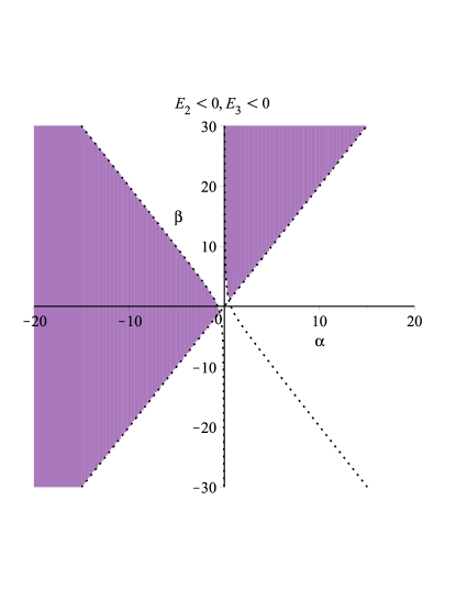
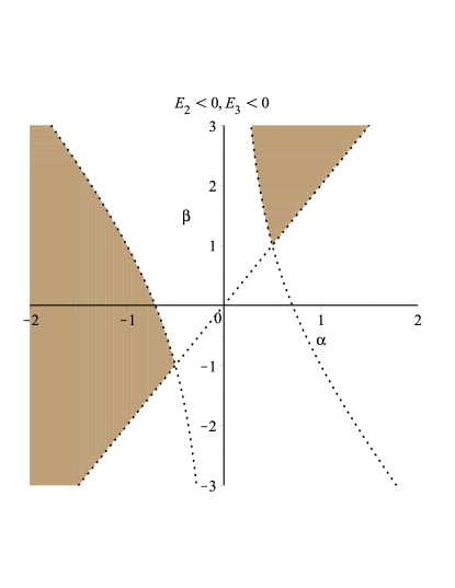
Figure 1: permissible values for $\alpha$ and $\beta$ parameters with stable state of the solutions (negative eigenvalues $E_{2,3}<0$)

The presence of a zero root $\varepsilon_{4}=0$ indicates that the system is degenerated at all and by adding some other perturbation sources may reaches to stable or unstable states and we will investigate this case as our future work. Regardless to this zero eigenvalue which can be resolve by considering a time evolution of the collapsing compact stellar object, we must set $\varepsilon_{1,2,3}<0$ for which $\varepsilon_{3}$ gives us $2\alpha<\beta$ and $\varepsilon_{2}$ gives us $4\alpha^{2}+2\alpha\beta-1>1.$ These inequalities are shown in figure 1 for permissable values of the parameters $\alpha,\beta$ which make $\varepsilon_{2,3}<0.$ For $\varepsilon_{1}<0$ we know that $n>0$ and so we must be choose $\gamma>-1.$ For instance if we set $\gamma=-\frac{1}{3}$ then the barotropic index for transverse pressure behaves as quintessence dark energy while for $\gamma=-\frac{2}{3}$ this behaves as fantom phase of the dark energy. For super fluid (supper sonic) the sound speed reaches to a maximum value such that $\gamma=1$ which we consider here such that $\varepsilon_{1}=\frac{-4}{1+n}.$ In the latter case we have degenerate state $\varepsilon_{0}=0$ for isothermal star with $n\to\infty$ and for constant density with $n=0$ we have $\varepsilon_{1}=-4$ while for star in convection equilibrium with $n=1.5$ we have $\varepsilon_{1}=-1.6.$ Furthermore in central region of a compact stellar objects we can consider the fluid behaves as isotropic and homogenous namely

$$\delta=\frac{p_{0r}}{\rho_{0}}=\gamma=\frac{p_{0t}}{\rho_{0}}.$$ (6.3)

In summary, by looking at the figure 1 we choose anstaz

$$\alpha=1,~{}~{}~{}\beta=3,~{}~{}~{}\gamma=\delta=1$$ (6.4)

for numerical studies in what follows and obtain

$$\varepsilon_{1}=\frac{-4}{1+n},~{}~{}~{}\varepsilon_{2}=-\frac{9}{8},~{}~{}~{}\varepsilon_{3}=-\frac{2}{3},~{}~{}~{}n>0$$ (6.5)

and

$$h_{1}=\frac{9}{8},~{}~{}~{}h_{2}=\frac{3}{8},~{}~{}~{}h_{3}=\frac{22}{24},~{}~{}~{}h_{4}=-\frac{3}{16},~{}~{}~{}h_{5}=-\frac{23}{48},~{}~{}~{}h_{6}=\frac{1}{4}$$ (6.6)

$$u_{c}=2,~{}~{}~{}z_{c}=1,~{}~{}~{}J_{11}=\frac{-1}{1+n},~{}~{}~{}J_{22}=-\frac{9}{8},~{}~{}~{}J_{33}=-\frac{2}{3},~{}~{}~{}J_{13}=\frac{-1}{1+n},$$

$$J_{32}=0,~{}~{}~{}J_{34}=\frac{4}{3},~{}~{}~{}J_{42}=\frac{1}{4},~{}~{}~{}A=-\frac{11}{18},~{}~{}~{}B=\frac{512}{99(9n-23)}$$

$$C=\frac{18}{11(5-n)}.$$

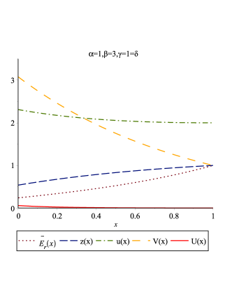
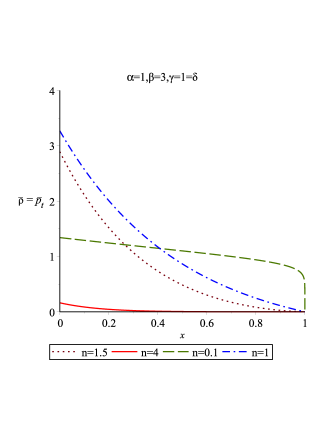
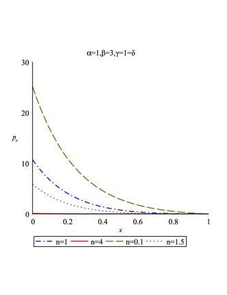
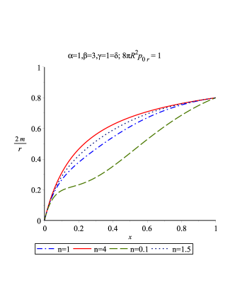
Figure 2: Diagrams of the fields for sample permissible values of the parameters $\alpha=1,\beta=3,\delta=\gamma=1$

For these numeric values we plotted dimensionless radial electric field $\bar{E}_{r}(x),$ dimensionless matter density $\bar{\rho}=\frac{\rho(x)}{\rho_{0}}$, dimensionless pressures $\bar{p}_{r}=\frac{p_{r}}{p_{0r}}$ and $\bar{p}_{t}=\frac{p_{t}}{p_{0t}}$ and mass per radius relation $\frac{2m}{r}$ in figures 2 for different values of the polytropic index $n$ parameter. By looking at the figure 2-a one can infer that by rasing the radial distance the electric field intensity increases and take on its maximum value on the surface of star. While internal metric components decreases. The figure 2-b shows that decreasing slope of the density function decreases faster by raising he radial distance of the star from its center and vanishes on the star surface. There is similar behavior for the transverse pressure and radial pressure but with larger scale. For smallest value of the polytropic index $n$ slope of density diagram by raising the radial distance of the star is very slow but it is dropped suddenly near the star radius. The figure 2-d shows variations of the mass per radius relation of the compact star with positive slope such that its maximum value does not reach to Schwarzschild radius means that our obtained stellar object is really an visible star and not a black hole. In summary, by looking at these diagrams one can infer that the obtained solutions describe a electrostatic spherically symmetric anisotropic star with maximal stability at classical regimes of the field. This results obey results of the quantum regimes of the field given in the ref. [14] which is investigated recently by one of us. In the next section discuss outputs of the work and future ideas for extension of the work.

7 Concluding remarks

In this work we added a nonminimal directionally interaction Lagrangian between geometry and the electromagnetic vector potential for Einstein-Maxwell gravity and investigated this additional contribution on internal space time of spherically symmetric static stellar compact object. After to solve the Euler-Lagrange equations of the fields via dynamical systems approach, we determined stabilization conditions of the obtained solutions near parametric critical points in phase space. We obtained permissable numeric values of the parameters of the interaction Lagrangian parts which give stable nature for the obtained solutions. This results are found by determining sign of eigenvalues of the Jacobi matrix of the dynamical equations of the system. One of the four eigenvalues is zero value while other tree eigenvalues were parametric which by choosing suitable numeric values for the parameters they become negative sign. However in the dynamical system approach the system become full stable if all eigenvalues become negative real numbers. If one of the is zero then the system become quasi stable. Hence to make negative values for zero eigenvalue we should consider other sources which can be break this degeneracy. This will done in our future work by considering the magnetic field (see [15] for magnetic monopole application). However by choosing a polytropic form of the equation of state we show that the stability of the system is dependent to particular values of the polytropic index of the system together with the two coupling constant of the gravity model under consideration.

8 Appendix I

$$\Sigma =8\alpha^{3}\beta+4\alpha^{2}\beta^{2}-4\alpha\beta$$

$$r[(8\alpha^{2}-8\alpha^{4}-8\alpha^{3}\beta+2\alpha^{2}\beta^{2}+2\alpha\beta^{3})f$$

$$+(2\alpha\beta-8\alpha^{4}-8\alpha^{3}\beta-2\alpha^{2}\beta^{2}+V\beta^{2}+2\alpha^{2}\beta+\alpha\beta^{2}+8\alpha^{2})\psi]$$ (8.1)

$$\Sigma_{V} =(4\alpha^{3}\beta+2\alpha^{2}\beta^{2}-\alpha\beta)V-4\alpha^{3}\beta-2\alpha^{2}\beta^{2}+\alpha\beta$$

$$r[(16\alpha^{4}+16\alpha^{3}\beta+4\alpha^{2}\beta^{2}+4\alpha^{2}\beta-16\alpha^{2}+2\alpha\beta)\psi$$

$$+(16\alpha^{4}+16\alpha^{3}\beta+4\alpha^{2}\beta^{2}-6\alpha^{2}\beta+\alpha\beta^{2}-16\alpha^{2}+10\alpha\beta-\beta^{2})f]$$

$$r^{2}[(-4\alpha^{3}-2\alpha^{2}\beta-4\alpha\beta-2\beta^{2}+4\alpha)\psi^{2}+(-8\alpha^{4}-24\alpha^{3}\beta-18\alpha^{2}\beta^{2}$$

$$-4\alpha\beta^{3}-11\alpha^{2}\beta-4\alpha\beta^{2}+8\alpha^{2}+15\alpha\beta-2\beta^{2})f\psi$$

$$+((8\alpha^{4}+8\alpha^{3}\beta+2\alpha^{2}\beta^{2}-8\alpha^{2}+\alpha\beta)p_{r}-\alpha\beta\rho)V$$

$$+(-8\alpha^{4}-16\alpha^{3}\beta-18\alpha^{2}\beta^{2}-6\alpha\beta^{3}+8\alpha^{2}+17\alpha\beta-6\beta^{2})f^{2}]$$ (8.2)

$$\Sigma_{f} =\psi[(8\alpha^{4}+4\alpha^{3}\beta-2\alpha^{2})V+24\alpha^{4}+12\alpha^{3}\beta-14\alpha^{2}]$$

$$+f[(8\alpha^{4}-2\alpha^{2}\beta^{2}-2\alpha^{2}+\alpha\beta)V+24\alpha^{4}-6\alpha^{2}\beta^{2}-14\alpha^{2}+7\alpha\beta]$$

$$+r[f^{2}(-16\alpha^{4}-32\alpha^{3}\beta-20\alpha^{2}\beta^{2}-4\alpha\beta^{3}-12\alpha^{3}+8\alpha^{2}\beta-\alpha\beta^{2}$$

$$+28\alpha^{2}+8\alpha\beta+\beta^{2})+\psi f(-16\alpha^{4}-24\alpha^{3}\beta-8\alpha^{2}\beta^{2}+4V\alpha\beta-2V\beta^{2}$$

$$+4\alpha^{3}-2\alpha^{2}\beta-2\alpha\beta^{2}+40\alpha^{2}+8\alpha\beta)+(16\alpha^{4}+8\alpha^{3}\beta-8\alpha^{2})Vp_{r}$$

$$+4V\alpha\beta\psi^{2}+(8\alpha^{3}+12\alpha^{2}+4\alpha)\psi^{2}]+r^{2}[f^{3}(32\alpha^{4}+16\alpha^{3}\beta-8\alpha^{2}\beta^{2}$$

$$-4\alpha\beta^{3}-14\alpha^{2}-29\alpha\beta+6\beta^{2})+f^{2}\psi(32\alpha^{4}+24\alpha^{3}\beta-4\alpha^{2}\beta^{2}$$

$$-4\alpha\beta^{3}-2V\alpha\beta-5V\beta^{2}-26\alpha^{3}-9\alpha^{2}\beta-\alpha\beta^{2}-20\alpha^{2}-41\alpha\beta+2\beta^{2})$$

$$f\psi^{2}(-2V\alpha\beta-4V\beta^{2}-18\alpha^{3}-18\alpha^{2}\beta-6\alpha\beta^{2}-14\alpha^{2}-12\alpha\beta+2\beta^{2}$$

$$-4\alpha)+fV\rho(-2\alpha^{2}+\alpha\beta)+fVp_{r}(-8\alpha^{4}+2\alpha^{2}\beta^{2}+10\alpha^{2}-\alpha\beta)]$$

$$\Sigma_{\psi} =4\alpha^{2}\beta(1-V)+r[(8\alpha^{2}\beta^{2}+20\alpha^{3}-26\alpha^{2}\beta-9\alpha\beta)\psi+\psi V(12\alpha^{3}+2\alpha^{2}\beta$$

$$-2\alpha\beta^{2}+\alpha\beta)+2\psi V^{3}\alpha\beta^{2}+f\psi(24\alpha^{3}\beta-4\alpha^{2}\beta^{2}+20\alpha^{3}-54\alpha^{2}\beta+2\alpha\beta^{2})$$

$$+fV\psi(12\alpha^{3}-2\alpha^{2}\beta+2\alpha\beta^{2})]+r^{2}[(16\alpha^{3}-12\alpha^{2}\beta)Vp_{r}+(-24\alpha^{4}-8\alpha^{3}\beta$$

$$+14\alpha^{2}\beta^{2}-2\alpha\beta^{3}+24\alpha^{3}+4\alpha^{2}\beta+26\alpha\beta^{2}+2\beta^{3})f^{2}+fV\psi(8\alpha^{2}\beta+4\alpha\beta^{2})$$

$$+(-24\alpha^{4}+20\alpha^{3}\beta+10\alpha^{2}\beta^{2}+4\alpha\beta^{3}+48\alpha^{3}+46\alpha^{2}\beta+17\alpha\beta^{2}+32\alpha^{2}$$

$$-6\alpha\beta+\beta^{2})\psi f+(8\alpha^{2}\beta+4\alpha\beta^{2}+2\beta^{2})\psi^{2}V+4\alpha^{2}\beta\rho V+(-8\alpha^{3}\beta-4\alpha^{2}\beta^{2}$$

$$+24\alpha^{3}+28\alpha^{2}\beta+10\alpha\beta^{2}+24\alpha^{2}+2\alpha\beta)\psi^{2}]+r^{3}[(4\alpha^{2}\beta+2\alpha\beta^{2})V^{2}\psi p_{r}$$

$$+(12\alpha^{3}+6\alpha^{2}\beta+8\alpha^{2}-\alpha\beta)V\psi p_{r}+(4\alpha^{3}+18\alpha^{2}\beta-2\alpha\beta^{2})Vfp_{r}$$

$$+(-2V\alpha\beta-16\alpha^{3}-16\alpha^{2}\beta-4\alpha\beta^{2}+4\alpha^{2}+4\alpha\beta+2\beta^{2}-4\alpha)\psi^{3}$$

$$+(-36\alpha^{4}-30\alpha^{3}\beta-6\alpha^{2}\beta^{2}-28\alpha^{3}-37\alpha^{2}\beta-5\alpha\beta^{2}+4\beta^{3}-8\alpha^{2}$$

$$-25\alpha\beta+2\beta^{2})f\psi^{2}+(-4\alpha^{2}\beta-10\alpha\beta^{2}-4\beta^{3}-\beta^{2})Vf\psi^{2}$$

$$+(-36\alpha^{4}-30\alpha^{3}\beta+12\alpha^{2}\beta^{2}+6\alpha\beta^{3}+24\alpha^{3}-76\alpha^{2}\beta-58\alpha\beta^{2}$$

$$+4\beta^{3}-16\alpha^{2}-17\alpha\beta+6\beta^{2})f^{2}\psi+(-4\alpha^{2}\beta-6\alpha\beta^{2}-6\beta^{3})f^{2}\psi V$$

$$+(-4\alpha^{3}-2\alpha^{2}\beta+\alpha\beta)\rho\psi V+(36\alpha^{3}-54\alpha^{2}\beta-46\alpha\beta^{2}+12\beta^{3})f^{3}$$

$$+(-4\alpha^{3}-2\alpha^{2}\beta+2\alpha\beta^{2})\rho Vf]$$ (8.4)

and

$$\Sigma_{p_{t}} =(16\alpha^{5}+16\alpha^{4}\beta+4\alpha^{3}\beta^{2}-4\alpha^{3}-2\alpha^{2}\beta)V\psi$$

$$+(48\alpha^{5}-12\alpha^{3}\beta^{2}-28\alpha^{3}+10\alpha^{2}\beta)\psi$$

$$+(16\alpha^{5}+20\alpha^{4}\beta+6\alpha^{3}\beta^{2}-4\alpha^{3}-3\alpha^{2}\beta)Vf$$

$$+(48\alpha^{5}-36\alpha^{4}\beta-30\alpha^{3}\beta^{2}-28\alpha^{3}+27\alpha^{2}\beta)f$$

$$+r[(64\alpha^{5}+64\alpha^{4}\beta+16\alpha^{3}\beta^{2}-24\alpha^{4}-14\alpha^{3}\beta+3\alpha^{2}\beta^{2}$$

$$-40\alpha^{3}+50\alpha^{2}\beta-15\alpha\beta^{2})f^{2}+(8\alpha^{2}\beta-6\alpha\beta^{2})V\psi f$$

$$+((8\alpha^{2}\beta-6\alpha\beta^{2})V+10\alpha^{2}\beta-10\alpha\beta^{2}+160\alpha^{4}\beta+60\alpha^{3}\beta^{2}$$

$$+4\alpha^{2}\beta^{3}-4\alpha^{2}\beta^{2}+112\alpha^{5}+8\alpha^{4}-64\alpha^{3})\psi f$$

$$+(8\alpha^{2}\beta-2\alpha\beta^{2})V\psi^{2}+(48\alpha^{5}+80\alpha^{4}\beta+28\alpha^{3}\beta^{2}+16\alpha^{4}$$

$$+12\alpha^{3}\beta+2\alpha^{2}\beta^{2}-24\alpha^{3}-16\alpha^{2}\beta+8\alpha^{2}-4\alpha\beta)\psi^{2}$$

$$+(32\alpha^{5}+8\alpha^{4}\beta-4\alpha^{3}\beta^{2}-16\alpha^{3}+4\alpha^{2}\beta)Vp_{r}]$$

$$+r^{2}[(-4\alpha^{3}-2\alpha^{2}\beta)\psi V\rho+(-4\alpha^{3}-3\alpha^{2}\beta)fV\rho+(4\alpha^{2}\beta-\alpha\beta^{2})\psi V^{2}p_{r}$$

$$+(24\alpha^{5}+24\alpha^{4}\beta+6\alpha^{3}\beta^{2}+8\alpha^{4}+2\alpha^{3}\beta-\alpha^{2}\beta^{2}-12\alpha^{3})\psi Vp_{r}$$

$$+(32\alpha^{5}+48\alpha^{4}\beta+12\alpha^{3}\beta^{2}-2\alpha^{2}\beta^{3}-28\alpha^{3}+3\alpha^{2}\beta)fVp_{r}$$

$$+(4\alpha\beta^{2}-2\alpha\beta+\beta^{2})\psi^{3}V+(-4\alpha^{2}\beta+2\beta^{3})f\psi^{2}V$$

$$+(-4\alpha^{2}\beta-6\alpha\beta^{2}+3\beta^{3})f^{2}\psi V$$

$$+(-32\alpha^{5}-32\alpha^{4}\beta-8\alpha^{3}\beta^{2}-8\alpha^{4}+2\alpha^{2}\beta^{2}+12\alpha^{3}$$

$$-8\alpha^{2}\beta-3\alpha\beta^{2}+12\alpha^{2}+2\alpha\beta)\psi^{3}$$

$$+(-112\alpha^{5}-160\alpha^{4}\beta-60\alpha^{3}\beta^{2}-4\alpha^{2}\beta^{3}-64\alpha^{4}$$

$$-60\alpha^{3}\beta-6\alpha^{2}\beta^{2}+4\alpha\beta^{3}+84\alpha^{3}+18\alpha^{2}\beta-6\alpha\beta^{2}+20\alpha^{2})f\psi^{2}$$

$$+(-88\alpha^{5}-240\alpha^{4}\beta-166\alpha^{3}\beta^{2}-26\alpha^{2}\beta^{3}+4\alpha\beta^{4}-52\alpha^{4}$$

$$-65\alpha^{3}\beta-12\alpha^{2}\beta^{2}+3\alpha\beta^{3}+112\alpha^{3}+75\alpha^{2}\beta-12\alpha\beta^{2})f^{2}\psi$$

$$+(-8\alpha^{5}-104\alpha^{4}\beta-122\alpha^{3}\beta^{2}-24\alpha^{2}\beta^{3}$$

$$+6\alpha\beta^{4}+44\alpha^{3}+51\alpha^{2}\beta-18\alpha\beta^{2})f^{3}].$$ (8.5)

References

- [1] F. Sandin, P. Ciarcelluti, ‘ Effects of mirror dark matter on neutron stars‘, Astroparticle Physics Volume 32, Issue 5, Pages 278-284 (2009); arXiv:0809.2942 [astro-ph]
- [2] J. Kumar and P. Bharti, ‘An isotropic compact stellar model in curvature coordinate system consistent with observational data‘, arXiv:2102.12754 [astro-ph.GA]
- [3] J. D. V. Arbañil, ‘M. Malheiro, Equilibrium and stability of charged strange quark stars‘ ,Phys. Rev. D 92, 084009 (2015); arXiv:1509.07692 [astro-ph.SR]
- [4] P. Bhar, P. Rej, P. Mafa Takisa, M. Zubair,‘Relativistic compact stars in Tolman spacetime via an anisotropic approach‘ Eur. Phys. J. C, vol81, 531, (2021); arXiv:2106.10425 [gr-qc]
- [5] G. Panotopoulos, A. Rincon, I. Lopes, ‘Interior solutions of relativistic stars with anisotropic matter in scale-dependent gravity‘, Eur. Phys. J. C vol81, 63, (2021); arXiv:2101.06649 [gr-qc]
- [6] D.S. Fontanella and A. Cabo, ‘A stability analysis of the static EKG Boson Stars‘, arXiv:2101.04681 [gr-qc]
- [7] B. Dayanandan, S.K. Maurya, S. T. T, ‘Modeling of charged anisotropic compact stars in general relativity‘, Eur. Phys. J. A vol53, 141, (2017); arXiv:1611.00320 [gr-qc]
- [8] J. D. V. Arbail, M. Malheiro, ‘Equilibrium and stability of charged strange quark stars‘, Phys. Rev. D 92, 084009 (2015); arXiv:1509.07692 [astro-ph.SR]
- [9] J. C. Jimnez, E. S. Fraga, ‘Radial oscillations in neutron stars from QCD‘, Phys. Rev. D 104, 014002 (2021); arXiv:2104.13480 [hep-ph]
- [10] B. Kain, ‘Fermion-charged-boson stars‘, Phys. Rev. D 104, 043001 ( 2021); arXiv:2108.01404 [gr-qc]
- [11] W. Wang, Y. Feng, X. Lai, Y. Li, J. Lu, X. Chen and R. Xu, ‘The optical/UV excess of X-ray-dim isolated neutron star II. nonuniformity of plasma on strangeon star surface‘,Res. Astron. Astrophys. 18 082 (2018), arXiv:1705.03763 [astro-ph.HE]
- [12] W. Wang, J. Lu, H. Tong, M. Ge, Z. Li, Y. Men, R. Xu, ‘The optical/UV excess of X-ray dim isolated neutron star: I. bremsstrahlung emission from a strangeon star plasma atmosphere‘,ApJ 837 81 (2017), arXiv:1603.08288 [astro-ph.HE]
- [13] M. S. Turner and L. M. Widrow, ‘Inflation Produced, Large Scale Magnetic Fields‘, Phys.Rev. D 37, 2743 (1988).
- [14] H. Ghaffarnejad, ‘Canonical quantization of modified non-gauge invariant Einstein-Maxwell gravity and stability of spherically symmetric electrostatic stars‘, Phys. Scr.98, 075018, (2023); arXiv:2306.10285 [gr-qc]
- [15] H. Ghaffarnejad and L. Naderi, ‘Modified Gauge Invariance Einstein Maxwell Gravity and Stability of Spherical Stars with Magnetic Monopoles ‘, arXiv:2212.09485 [gr-qc]
- [16] H. Ghaffarnejad, E. Yaraie,‘Dynamical system approach to scalar-vector-tensor cosmology‘,Gen. Relativ Gravit 49, 49 (2017); arXiv:1604.06269 [physics.gen-ph]
- [17] H. Ghaffarnejad and H. Gholipour, ‘Bianchi I metric solutions with nonminimally coupled Einstein-Maxwell gravity theory‘, Gen. Relativ. Gravit 53, 1 (2021); arXiv:2003.14216 [gr-qc]
- [18] C. Catton, T. Faber and M. Visser, ‘Gravastars must have anisotropic pressures‘, Class. Quant. Grav.22:4189 (2005): gr-qc/0505137.
- [19] M. P. Hobson, G. P. Erstathiou and A. N. Lasenby ‘General Relativity‘ An Introduction for Physicists, Cambridge University Press (2006).