Parametric “Non-nested” Discriminants
for Multiplicities of Univariate Polynomials

Abstract

We consider the problem of complex root classification, i.e., finding the conditions on the coefficients of a univariate polynomial for all possible multiplicity structures on its complex roots. It is well known that such conditions can be written as conjunctions of several polynomial equations and one inequation in the coefficients. Those polynomials in the coefficients are called discriminants for multiplicities. It is also known that discriminants can be obtained by using repeated parametric gcd’s. The resulting discriminants are usually nested determinants, that is, determinants of matrices whose entries are determinants, and so on. In this paper, we give a new type of discriminants which are not based on repeated gcd’s. The new discriminants are simpler in the sense that they are non-nested determinants and have smaller maximum degrees.

12D10, 68W30

1 Introduction

In this paper, we consider the problem of complex root classification, i.e., finding the conditions on the coefficients of a polynomial over the complex field $\mathbb{C}$ for every potential multiplicity structure its complex roots may have. For example, consider a quintic polynomial $F=a_{5}x^{5}+a_{4}x^{4}+a_{3}x^{3}+a_{2}x^{2}+a_{1}x+a_{0}$ where $a_{i}$’s take values over $\mathbb{C}$. We would like to find conditions $C_{0},C_{1},\ldots,C_{6}$ on $a=(a_{0},\ldots,a_{5})$ such that

$$\text{multiplicity structure of }F=\left\{\begin{array}[c]{lll}\left(1,1,1,1,1\right),&\text{if }&C_{0}\left(a\right)\ \text{holds;}\\ (2,1,1,1),&\text{if}&C_{1}\left(a\right)\ \text{holds};\\ (2,2,1),&\text{if}&C_{2}\left(a\right)\ \text{holds};\\ (3,1,1),&\text{if}&C_{3}\left(a\right)\ \text{holds};\\ (3,2),&\text{if}&C_{4}\left(a\right)\ \text{holds};\\ \left(4,1\right),&\text{if}&C_{5}\left(a\right)\ \text{holds};\\ \left(5\right),&\text{if}&C_{6}\left(a\right)\ \text{holds}.\end{array}\right.$$

In general, the problem is stated as follows:

Problem: For every $\bm{\mu}=\left(\mu_{1},\ldots,\mu_{m}\right)$ such that $\mu_{1}\geq\ldots\geq\mu_{m}>0$ and $\mu_{1}+\cdots+\mu_{m}=n$, find a condition on the coefficients of a polynomial $F$over $\mathbb{C}$ of degree $n$ such that the multiplicity structure of $F$ is $\bm{\mu}$.

The problem is important because many tasks in mathematics, science and engineering can be reduced to the problem. Due to its importance, the problem and several related problems have been already carefully studied [5, 7, 8, 9, 10, 13].

The problem can be viewed as a generalization of the well known problem of finding a condition on coefficients such that the polynomial has the given number of distinct roots. This subproblem has been extensively studied. For instance, the subdiscriminant theory provides a complete solution to the subproblem: a univariate polynomial of degree $n$ has $m$ distinct roots if and only if its $0$-th, $\ldots$, $(n-m-1)$-th psd’s (i.e., principal subdiscriminant coefficient) vanish and the $(n-m)$-th psd does not. For details, see standard textbooks on computational algebra (e.g., [1]).

In [13], Yang, Hou and Zeng gave an algorithm to generate conditions for discriminating different multiplicity structures of a univariate polynomial (referred as YHZ’s condition hereinafter) by making use of repeated gcd computation for parametric polynomials [3, 4, 11]. It is based on a similar idea adopted by Gonzalez-Vega et al. [5] for solving the real root classification and quantifier elimination problems by using Sturm-Habicht sequences. The conditions produced by these methods are conjunctions of several polynomial equations and one inequation on the coefficients. Those polynomials in the coefficients are called discriminants for multiplicities. The maximum degree of the discriminants grows exponentially in the degree of $F$. Furthermore, each discriminant is a “nested” determinant, that is, it is a determinant of a matrix whose entries are again determinants and so on.

In [7], the authors developed a new type of multiplicity discriminants to distinguish different multiplicities when the number of distinct roots is fixed. The main idea is to convert the multiplicity condition expressed as a permanent inequation in roots into a sum of determinants in coefficients. In order to generate conditions for all the possible multiplicity structures of a univariate polynomial, one may first use subdiscriminants in classical resultant theory to decide the number of distinct complex roots and then add one more inequation to discriminate different multiplicity structures with the same number of distinct roots. In the new condition, the maximum degree of the discriminants grows linearly in the degree of $F$, which makes the size of discriminants significantly smaller. However, the form of resulting discriminants is a sum of many determinants, which makes the further analysis (reasoning) difficult.

The main contribution in this paper is to provide a new type of discriminants, which are non-nested determinants and whose maximum degrees are smaller than those in the previous methods. The method is based on a significantly different theory and techniques from the previous methods (which are essentially based on repeated parametric gcd or subdiscriminant theory). The new condition is given by a newly devised multiplicity discriminant in coefficients for every potential multiplicity vector of a given degree, which can be viewed as a generalization of subdiscriminant theory to higher order derivatives. To build up the connection between the new discriminants and multiple roots, we first convert it into the ratio of two determinants in terms of generic roots (without considering the multiplicities). Then by making use of the connection between divided difference with multiple nodes and the derivatives of higher orders at the nodes, we integrate the multiplicity information into the expression and convert it into an expression in terms of multiple roots. After careful manipulation, it is shown that the new discriminant can capture the multiplicity information.

The paper is structured as follows. In Section 2, we first present the problem to be solved in a formal way. In Section 3, we give a precise statement of the main result of the paper (Theorem 3.5). Then a proof of Theorem 3.5 is provided in Section 4. The proof is long thus we divide the proof into three subsections which are interesting on their own. In Section 5, we compare the form and size of polynomials in the multiplicity-discriminant condition in Theorem 3.5 and those given by previous works.

2 Problem

Definition 2.1 (Multiplicity vector).

Let $F\in\mathbb{C}\left[x\right]$ with $m$ distinct complex roots, say $r_{1},\ldots,r_{m}$, with multiplicities $\mu_{1},\ldots,\mu_{m}$ respectively. Without losing generality, we assume that $\mu_{1}\geq\cdots\geq\mu_{m}>0$. Then the multiplicity vector of $F$, written as $\operatorname*{mult}\left(F\right)$, is defined by

$$\operatorname*{mult}\left(F\right)=\left(\mu_{1},\ldots,\mu_{m}\right).$$

Example 2.2.

Let $F=x^{5}-5x^{4}+7x^{3}+x^{2}-8x+4$. Then $\operatorname*{mult}\left(F\right)=\left(2,2,1\right)$, since it can be verified that $F$ $=\left(x-1\right)^{2}\left(x+1\right)^{1}\left(x-2\right)^{2}$. Note that the multiplicity vector is a partition of $5,$ which is the degree of $F$.

Definition 2.3 (Potential multiplicity vectors).

Let $n$ be a positive integer. Let $\mathcal{M}(n)$ stand for the set of all the potential multiplicity vectors of polynomials of degree $n$, equivalently, the set of all partitions of $n,$ that is,

$$\mathcal{M}(n)=\left\{(\mu_{1},\ldots,\mu_{m}):\,\mu_{1}+\cdots+\mu_{m}=n,\mu_{1}\geq\cdots\geq\mu_{m}>0\right\}.$$

Example 2.4.

$\mathcal{M}\left(5\right)=\left\{\ \left(1,1,1,1,1\right),\ \ \left(2,1,1,1\right),\ \left(2,2,1\right),\ \left(3,1,1\right),\ \left(3,2\right),\ \left(4,1\right),\ \left(5\right)\ \right\}$.

Problem 2.5 (Parametric multiplicity problem).

The parametric multiplicity problem is stated as:

1. $n$, a positive integer standing for the polynomial of degree $n$ with parametric coefficients $a$, that is,

   $$F=\sum_{i=0}^{n}a_{i}x^{i}\ \ \text{where}\ \ a_{n}\neq 0.$$

2. For each $\bm{\mu}\in\mathcal{M}(n)$, find a condition $C_{\bm{\mu}}\$on $a\$such that $\operatorname*{mult}\left(F\right)=\bm{\mu}$.

3 Main Result

Definition 3.1 (Determinant polynomial).

Consider a vector of univariate polynomials

$$P=\left[\begin{array}[c]{c}P_{0}\\ \vdots\\ P_{k}\end{array}\right]\in\mathbb{C}[x]^{k+1}$$

where $\deg P_{i}\leq k\ \ \text{and}\ \ P_{i}=\sum_{0\leq j\leq k}a_{ij}x^{j}.$ The coefficient matrix of $P,$ written as $C\left(P\right),$ is defined by

$$C\left(P\right)=\operatorname*{coef}\left(P\right)=\begin{bmatrix}\operatorname*{coef}\left(P_{0}\right)\\ \vdots\\ \operatorname*{coef}\left(P_{k}\right)\end{bmatrix}=\begin{bmatrix}a_{0k}&\cdots&a_{00}\\ \vdots&&\vdots\\ a_{kk}&\cdots&a_{k0}\end{bmatrix}.$$

The determinant polynomial of $P,$ written as $\operatorname*{dp}\left(P\right),$ is defined by

$$\operatorname*{dp}\left(P\right)=|C\left(P\right)|.$$

Definition 3.2 (Multiplicity Discriminant).

Let $F=\sum_{i=0}^{n}a_{i}x^{i}\ \$where$\ \ a_{n}\neq 0$. Let $\bm{\gamma}=\left(\gamma_{1},\ldots,\gamma_{s}\right)\in\mathcal{M}\left(n\right)$. The the $\bm{\gamma}$-discriminant of $F$, written as $D\left(\bm{\gamma}\right),\$is defined by

$$D\left(\bm{\gamma}\right)=\frac{1}{a_{n}}\operatorname*{dp}\left[\begin{array}[c]{l}F^{(0)}x^{\gamma_{0}-1}\\ ~{}~{}~{}~{}\ \vdots\\ F^{(0)}x^{0}\\ \hline\cr F^{(1)}x^{\gamma_{1}-1}\\ ~{}~{}~{}~{}\ \vdots\\ F^{(1)}x^{0}\\ \hline\cr~{}~{}~{}~{}\ \vdots\\ \hline\cr F^{(s)}x^{\gamma_{s}-1}\\ ~{}~{}~{}~{}\ \vdots\\ F^{(s)}x^{0}\end{array}\right]$$

where $\gamma_{0}$ is the smallest so that the above matrix is square and $F^{(i)}$ is the $i$-th derivative of $F$ in terms of $x$. It is straightforward to show that $\gamma_{0}=\gamma_{1}-1$.

Example 3.3.

Let $n=5$ and $F=\sum_{i=0}^{n}a_{i}x^{i}$ and $a_{n}\neq 0$. Then

$$\begin{array}[c]{lll}D\left(5\right)&=&\operatorname*{dp}\left[\begin{array}[c]{l}F^{(0)}x^{3}\\ F^{(0)}x^{2}\\ F^{(0)}x^{1}\\ F^{(0)}x^{0}\\ \hline\cr F^{(1)}x^{4}\\ F^{(1)}x^{3}\\ F^{(1)}x^{2}\\ F^{(1)}x^{1}\\ F^{(1)}x^{0}\end{array}\right]=\dfrac{1}{a_{5}}\left|\begin{array}[c]{ccccccccc}a_{5}&a_{4}&a_{3}&a_{2}&a_{1}&a_{0}&&&\\ &a_{5}&a_{4}&a_{3}&a_{2}&a_{1}&a_{0}&&\\ &&a_{5}&a_{4}&a_{3}&a_{2}&a_{1}&a_{0}&\\ &&&a_{5}&a_{4}&a_{3}&a_{2}&a_{1}&a_{0}\\ \hline\cr 5a_{5}&4a_{4}&3a_{3}&2a_{2}&1a_{1}&&&&\\ &5a_{5}&4a_{4}&3a_{3}&2a_{2}&1a_{1}&&&\\ &&5a_{5}&4a_{4}&3a_{3}&2a_{2}&1a_{1}&&\\ &&&5a_{5}&4a_{4}&3a_{3}&2a_{2}&1a_{1}&\\ &&&&5a_{5}&4a_{4}&3a_{3}&2a_{2}&1a_{1}\end{array}\right|,\\ D\left(4,1\right)&=&\operatorname*{dp}\left[\begin{array}[c]{l}F^{(0)}x^{2}\\ F^{\left(0\right)}x^{1}\\ F^{(0)}x^{0}\\ \hline\cr F^{(1)}x^{3}\\ F^{(1)}x^{2}\\ F^{(1)}x^{1}\\ F^{(1)}x^{0}\\ \hline\cr F^{(2)}x^{0}\end{array}\right]=\dfrac{1}{a_{5}}\left|\begin{array}[c]{cccccccc}a_{5}&a_{4}&a_{3}&a_{2}&a_{1}&a_{0}&&\\ &a_{5}&a_{4}&a_{3}&a_{2}&a_{1}&a_{0}&\\ &&a_{5}&a_{4}&a_{3}&a_{2}&a_{1}&a_{0}\\ \hline\cr 5a_{5}&4a_{4}&3a_{3}&2a_{2}&1a_{1}&&&\\ &5a_{5}&4a_{4}&3a_{3}&2a_{2}&1a_{1}&&\\ &&5a_{5}&4a_{4}&3a_{3}&2a_{2}&1a_{1}&\\ &&&5a_{5}&4a_{4}&3a_{3}&2a_{2}&1a_{1}\\ \hline\cr&&&&5\cdot 4a_{5}&4\cdot 3a_{4}&3\cdot 2a_{3}&2\cdot 1a_{2}\end{array}\right|,\\ D\left(3,2\right)&=&\operatorname*{dp}\left[\begin{array}[c]{l}F^{(0)}x^{1}\\ F^{(0)}x^{0}\\ \hline\cr F^{(1)}x^{2}\\ F^{(1)}x^{1}\\ F^{(1)}x^{0}\\ \hline\cr F^{(2)}x^{1}\\ F^{(2)}x^{0}\end{array}\right]=\dfrac{1}{a_{5}}\left|\begin{array}[c]{ccccccc}a_{5}&a_{4}&a_{3}&a_{2}&a_{1}&a_{0}&\\ &a_{5}&a_{4}&a_{3}&a_{2}&a_{1}&a_{0}\\ \hline\cr 5a_{5}&4a_{4}&3a_{3}&2a_{2}&1a_{1}&&\\ &5a_{5}&4a_{4}&3a_{3}&2a_{2}&1a_{1}&\\ &&5a_{5}&4a_{4}&3a_{3}&2a_{2}&1a_{1}\\ \hline\cr&&5\cdot 4a_{5}&4\cdot 3a_{4}&3\cdot 2a_{3}&2\cdot 1a_{2}&\\ &&&5\cdot 4a_{5}&4\cdot 3a_{4}&3\cdot 2a_{3}&2\cdot 1a_{2}\end{array}\right|,\end{array}$$

$$\begin{array}[c]{lll}D\left(3,1,1\right)&=&\operatorname*{dp}\left[\begin{array}[c]{l}F^{(0)}x^{1}\\ F^{(0)}x^{0}\\ \hline\cr F^{(1)}x^{2}\\ F^{(1)}x^{1}\\ F^{(1)}x^{0}\\ \hline\cr F^{(2)}x^{0}\\ \hline\cr F^{(3)}x^{0}\end{array}\right]=\dfrac{1}{a_{5}}\left|\begin{array}[c]{ccccccc}a_{5}&a_{4}&a_{3}&a_{2}&a_{1}&a_{0}&\\ &a_{5}&a_{4}&a_{3}&a_{2}&a_{1}&a_{0}\\ \hline\cr 5a_{5}&4a_{4}&3a_{3}&2a_{2}&1a_{1}&&\\ &5a_{5}&4a_{4}&3a_{3}&2a_{2}&1a_{1}&\\ &&5a_{5}&4a_{4}&3a_{3}&2a_{2}&1a_{1}\\ \hline\cr&&&5\cdot 4a_{5}&4\cdot 3a_{4}&3\cdot 2a_{3}&2\cdot 1a_{2}\\ \hline\cr&&&&5\cdot 4\cdot 3a_{5}&4\cdot 3\cdot 2a_{4}&3\cdot 2\cdot 1a_{3}\end{array}\right|,\\ D\left(2,2,1\right)&=&\operatorname*{dp}\left[\begin{array}[c]{l}F^{(0)}x^{0}\\ \hline\cr F^{(1)}x^{1}\\ F^{(1)}x^{0}\\ \hline\cr F^{(2)}x^{1}\\ F^{(2)}x^{0}\\ \hline\cr F^{(3)}x^{0}\end{array}\right]=\dfrac{1}{a_{5}}\left|\begin{array}[c]{cccccc}a_{5}&a_{4}&a_{3}&a_{2}&a_{1}&a_{0}\\ \hline\cr 5a_{5}&4a_{4}&3a_{3}&2a_{2}&1a_{1}&\\ &5a_{5}&4a_{4}&3a_{3}&2a_{2}&1a_{1}\\ \hline\cr&5\cdot 4a_{5}&4\cdot 3a_{4}&3\cdot 2a_{3}&2\cdot 1a_{2}&\\ &&5\cdot 4a_{5}&4\cdot 3a_{4}&3\cdot 2a_{3}&2\cdot 1a_{2}\\ \hline\cr&&&5\cdot 4\cdot 3a_{5}&4\cdot 3\cdot 2a_{4}&3\cdot 2\cdot 1a_{3}\end{array}\right|,\\ D\left(2,1,1,1\right)&=&\operatorname*{dp}\left[\begin{array}[c]{l}F^{(0)}x^{0}\\ \hline\cr F^{(1)}x^{1}\\ F^{(1)}x^{0}\\ \hline\cr F^{(2)}x^{0}\\ \hline\cr F^{(3)}x^{0}\\ \hline\cr F^{(4)}x^{0}\end{array}\right]=\dfrac{1}{a_{5}}\left|\begin{array}[c]{cccccc}a_{5}&a_{4}&a_{3}&a_{2}&a_{1}&a_{0}\\ \hline\cr 5a_{5}&4a_{4}&3a_{3}&2a_{2}&1a_{1}&\\ &5a_{5}&4a_{4}&3a_{3}&2a_{2}&1a_{1}\\ \hline\cr&&5\cdot 4a_{5}&4\cdot 3a_{4}&3\cdot 2a_{3}&2\cdot 1a_{2}\\ \hline\cr&&&5\cdot 4\cdot 3a_{5}&4\cdot 3\cdot 2a_{4}&3\cdot 2\cdot 1a_{3}\\ \hline\cr&&&&5\cdot 4\cdot 3\cdot 2a_{5}&4\cdot 3\cdot 2\cdot 1a_{4}\end{array}\right|,\\ D\left(1,1,1,1,1\right)&=&\operatorname*{dp}\left[\begin{array}[c]{l}F^{(1)}x^{0}\\ \hline\cr F^{(2)}x^{0}\\ \hline\cr F^{(3)}x^{0}\\ \hline\cr F^{(4)}x^{0}\\ \hline\cr F^{\left(5\right)}x^{0}\end{array}\right]=\dfrac{1}{a_{5}}\left|\begin{array}[c]{cccccc}{5a_{5}}&{4a_{4}}&{3a_{3}}&{2a_{2}}&{1a_{1}}\\ \hline\cr&5\cdot 4a_{5}&4\cdot 3a_{4}&3\cdot 2a_{3}&2\cdot 1a_{2}\\ \hline\cr&&5\cdot 4\cdot 3a_{5}&4\cdot 3\cdot 2a_{4}&3\cdot 2\cdot 1a_{3}\\ \hline\cr&&&5\cdot 4\cdot 3\cdot 2a_{5}&4\cdot 3\cdot 2\cdot 1a_{4}\\ \hline\cr&&&&5\cdot 4\cdot 3\cdot 2\cdot 1a_{5}\end{array}\right|.\end{array}$$

Note that the last one $D\left(1,1,1,1,1\right)=5^{5}4^{4}3^{3}2^{2}1^{1}a_{5}^{4}$. Since $a_{5}\neq 0$, we see that $D\left(1,1,1,1,1\right)\neq 0$.

To present the main theorem, we recall the following definition for the conjugate of $\bm{\mu}\in\mathcal{M}(n)$.

Definition 3.4 (Conjugate).

Let $\bm{\mu}=\left(\mu_{1},\ldots,\mu_{m}\right)\in\mathcal{M}(n)$. Then the conjugate $\overline{\bm{\mu}}=\left(\overline{\mu}_{1},\ldots,\overline{\mu}_{s}\right)$ of $\bm{\mu}$ is defined by

$$s =\max_{1\leq i\leq m}\mu_{i}=\mu_{1},$$

$$\overline{\mu}_{i} =\#\left\{\mu_{j}:\mu_{j}\geq i\right\}\ \ \ \text{for }i=1,\ldots,s.$$

Theorem 3.5 (Main Result).

Let $F=\sum_{i=0}^{n}a_{i}x^{i}\ \$where$\ \ a_{n}\neq 0$. Let $\mathcal{M}(n)=\left\{\bm{\mu}_{0},\bm{\mu}_{1},\ldots,\bm{\mu}_{p}\right\}$ where the entries are ordered in the lexicographically decreasing order in their conjugates $\overline{\bm{\mu}_{i}}$’s. Then we have the following conditions for the multiplicity vectors.

$$\operatorname*{mult}(F)=\left\{\begin{array}[c]{llll}{\bm{\mu}_{0}},&\text{if }&{D}\left({\overline{\bm{\mu}_{0}}}\right)&\neq 0;\\ \ \vdots&\vdots&\ {\vdots}&\\ {\bm{\mu}_{p-1},}&\text{else\ if}&{D}\left({\overline{\bm{\mu}_{p-1}}}\right)&\neq 0;\\ {\bm{\mu}_{p},}&\text{else\ if}&{D}\left({\overline{\bm{\mu}_{p}}}\right)&\neq 0.\end{array}\right.$$

Equivalently,

$$\operatorname*{mult}(F)={\bm{\mu}_{i}}\ \ \ \Longleftrightarrow\ \ \ D\left({\overline{\bm{\mu}_{0}}}\right)=\cdots=D\left({\overline{\bm{\mu}_{i-1}}}\right)=0\wedge D\left({\overline{\bm{\mu}_{i}}}\right)\neq 0.$$

Example 3.6.

We have the following condition for each multiplicity vector for degree $5$.

$$\operatorname*{mult}(F)=\left\{\begin{array}[c]{llll}\left(1,1,1,1,1\right),&\text{if }&D\left(5\right)&\neq 0;\\ (2,1,1,1),&\text{else\ if}&{D}\left(4,1\right)&\neq 0;\\ (2,2,1),&\text{else\ if}&{D}\left(3,2\right)&\neq 0;\\ (3,1,1),&\text{else\ if}&{D}\left(3,1,1\right)&\neq 0;\\ (3,2),&\text{else\ if}&{D}\left(2,2,1\right)&\neq 0;\\ \left(4,1\right),&\text{else\ if}&{D}\left(2,1,1,1\right)&\neq 0;\\ \left(5\right),&\text{else\ if}&{D}\left(1,1,1,1,1\right)&\neq 0.\end{array}\right.$$

Equivalently, for instance,

$$\operatorname*{mult}(F)=\left(2,2,1\right)\ \ \ \Longleftrightarrow\ \ \ D\left(5\right)={D}\left(4,1\right)=0\wedge D\left(3,2\right)\neq 0.$$

Remark 3.7.

Note that ${\overline{\bm{\mu}_{p}}}=(1,\ldots,1)$ and

$${D}\left({\overline{\bm{\mu}_{p}}}\right)=\frac{1}{a_{n}}\left|\begin{array}[c]{cccc}na_{n}&\cdots&\cdots&1a_{1}\\ &n\left(n-1\right)a_{n}&\cdots&2\cdot 1a_{2}\\ &&\ddots&\vdots{}{}{}\\ &&&n\left(n-1\right)\cdots 1a_{n}\end{array}\right|=\prod_{i=1}^{n}i^{i}\cdot a_{n}^{n-1}\neq 0.$$

Hence the last condition is always satisfied and there is no need to check the condition.

4 Proof of the Main Theorem

Here is a high level view of the proof. We start with converting ${D}\left(\bm{\mu}\right)$ into the equivalent symmetric polynomials in generic roots (though displayed as a ratio of two determinants) which is easier to embed the multiplicity information. Then by making use of the connection between divided difference with multiple nodes and the derivatives of higher orders at the nodes, we convert the expression in generic roots to that in distinct roots with multiplicity information integrated. The theorem will be proved by eliminating the entries in the determinantal expression obtained from the second stage which may vanish under the given multiplicity structure.

4.1 Multiplicity discriminant in terms of roots

We first understand what the multiplicity discriminants look like in terms of roots. .

Notation 4.1.

$V(\alpha_{1},\ldots,\alpha_{n}):=\left|\begin{array}[c]{ccc}\alpha_{1}^{n-1}&\cdots&\alpha_{n}^{n-1}\\ \vdots&&\vdots\\ \alpha_{1}^{0}&\cdots&\alpha_{n}^{0}\end{array}\right|$.

Lemma 4.2 (Multiplicity discriminant in generic roots).

Let $F=a_{n}(x-\alpha_{1})\cdots(x-\alpha_{n})$ and $\bm{\gamma}=(\gamma_{1},\ldots,\gamma_{s})\in\mathcal{M}(n)$. Then

$$D(\bm{\gamma})=\dfrac{a_{n}^{\gamma_{1}-2}\cdot\left|\begin{array}[c]{lcl}F^{(1)}(\alpha_{1})\alpha_{1}^{\gamma_{1}-1}&\cdots&F^{(1)}(\alpha_{n})\alpha_{n}^{\gamma_{1}-1}\\ ~{}~{}~{}~{}~{}~{}~{}\vdots&&~{}~{}~{}~{}~{}~{}~{}\vdots\\ F^{(1)}(\alpha_{1})\alpha_{1}^{0}&\cdots&F^{(1)}(\alpha_{n})\alpha_{n}^{0}\\ \hline\cr~{}~{}~{}~{}~{}~{}~{}\vdots&&~{}~{}~{}~{}~{}~{}~{}\vdots\\ \hline\cr F^{(s)}(\alpha_{1})\alpha_{1}^{\gamma_{s}-1}&\cdots&F^{(s)}(\alpha_{n})\alpha_{n}^{\gamma_{s}-1}\\ ~{}~{}~{}~{}~{}~{}~{}\vdots&&~{}~{}~{}~{}~{}~{}~{}\vdots\\ F^{(s)}(\alpha_{1})\alpha_{1}^{0}&\cdots&F^{(s)}(\alpha_{n})\alpha_{n}^{0}\end{array}\right|}{V(\alpha_{1},\ldots,\alpha_{n})}.$$ (1)

Proof 4.3.

1. Since $\gamma_{1}\geq\cdots\geq\gamma_{s}$ and $\gamma_{0}=\gamma_{1}-1$, we have

   $$\deg(F^{(0)}x^{n-2})>\cdots>\deg(F^{(0)}x^{\gamma_{1}-1})>\max({\deg(F^{(0)}x^{\gamma_{0}-1}),\deg(F^{(1)}x^{\gamma_{1}-1}),\ldots,\deg(F^{(s)}x^{\gamma_{s}-1})}).$$

   Thus

   $$D(\bm{\gamma})=\frac{1}{a_{n}}\operatorname*{dp}\left[\begin{array}[c]{l}F^{(0)}x^{\gamma_{1}-2}\\ ~{}~{}~{}~{}\vdots\\ F^{(0)}x^{0}\\ \hline\cr F^{(1)}x^{\gamma_{1}-1}\\ ~{}~{}~{}~{}\vdots\\ F^{(1)}x^{0}\\ \hline\cr~{}~{}~{}~{}\vdots\\ \hline\cr F^{(s)}x^{\gamma_{s}-1}\\ ~{}~{}~{}~{}\vdots\\ F^{(s)}x^{0}\end{array}\right]=\frac{1}{a_{n}}\cdot a_{n}^{\gamma_{1}-n}\operatorname*{dp}\left[\begin{array}[c]{l}F^{(0)}x^{n-2}\\ ~{}~{}~{}~{}\vdots\\ F^{(0)}x^{\gamma_{1}-1}\\ F^{(0)}x^{\gamma_{1}-2}\\ ~{}~{}~{}~{}\vdots\\ F^{(0)}x^{0}\\ \hline\cr F^{(1)}x^{\gamma_{1}-1}\\ ~{}~{}~{}~{}\vdots\\ F^{(1)}x^{0}\\ \hline\cr~{}~{}~{}~{}\vdots\\ \hline\cr F^{(s)}x^{\gamma_{s}-1}\\ ~{}~{}~{}~{}\vdots\\ F^{(s)}x^{0}\end{array}\right]=a_{n}^{\gamma_{1}-n-1}\operatorname*{dp}\left[\begin{array}[c]{l}F^{(0)}x^{n-2}\\ ~{}~{}~{}~{}\vdots\\ F^{(0)}x^{0}\\ \hline\cr F^{(1)}x^{\gamma_{1}-1}\\ ~{}~{}~{}~{}\vdots\\ F^{(1)}x^{0}\\ \hline\cr~{}~{}~{}~{}\vdots\\ \hline\cr F^{(s)}x^{\gamma_{s}-1}\\ ~{}~{}~{}~{}\vdots\\ F^{(s)}x^{0}\end{array}\right].$$

2. Now we recall the following result from [7] which is the key for proving the lemma. Let $G_{1},\ldots,G_{n}\in\mathbb{C}\left[x\right]_{2n-2}$ where $\mathbb{C}\left[x\right]_{2n-2}$ consists of all the polynomials in $x$ with degree no greater than $2n-2$. Then

   $$\operatorname*{dp}\left[\begin{array}[c]{l}F^{(0)}x^{n-2}\\ ~{}~{}~{}~{}\vdots\\ F^{(0)}x^{0}\\ ~{}~{}~{}~{}G_{1}\\ ~{}~{}~{}~{}\vdots\\ ~{}~{}~{}~{}G_{n}\end{array}\right]=\dfrac{a_{n}^{n-1}\cdot\left|\begin{array}[c]{ccc}G_{1}(\alpha_{1})&\cdots&G_{1}(\alpha_{n})\\ \vdots&&\vdots\\ G_{n}(\alpha_{1})&\cdots&G_{n}\left(\alpha_{n}\right)\end{array}\right|}{V(\alpha_{1},\ldots,\alpha_{n})}.$$ (2)

3. After specializing $G_{1},\ldots,G_{n}$ in (2) with $F^{(1)}x^{\gamma_{1}-1},\ldots,F^{(1)}x^{0},\ldots,F^{(s)}x^{\gamma_{s}-1},\ldots,F^{(s)}x^{0}$, respectively, we have

   $$D(\bm{\gamma})=a_{n}^{\gamma_{1}-n-1}\cdot\dfrac{a_{n}^{n-1}\cdot\left|\begin{array}[c]{lcl}\left(F^{(1)}x^{\gamma_{1}-1}\right)(\alpha_{1})&\cdots&\left(F^{(1)}x^{\gamma_{1}-1}\right)(\alpha_{n})\\ ~{}~{}~{}~{}~{}~{}~{}\vdots&&~{}~{}~{}~{}~{}~{}~{}\vdots\\ \left(F^{(1)}x^{0}\right)(\alpha_{1})&\cdots&\left(F^{(1)}x^{0}\right)(\alpha_{n})\\ \hline\cr~{}~{}~{}~{}~{}~{}~{}\vdots&&~{}~{}~{}~{}~{}~{}~{}\vdots\\ \hline\cr\left(F^{(s)}x^{\gamma_{s}-1}\right)(\alpha_{1})&\cdots&\left(F^{(s)}x^{\gamma_{s}-1}\right)(\alpha_{n})\\ ~{}~{}~{}~{}~{}~{}~{}\vdots&&~{}~{}~{}~{}~{}~{}~{}\vdots\\ \left(F^{(s)}x^{0}\right)(\alpha_{1})&\cdots&\left(F^{(s)}x^{0}\right)(\alpha_{n})\end{array}\right|}{V(\alpha_{1},\ldots,\alpha_{n})}$$

   which can be easily simplified into (1).

Remark 4.4.

It is very important to note that the right hand side is a polynomial function in $\alpha_{1},\ldots,\alpha_{n}$, even though written as a rational function, since the numerator is exactly divisible by the denominator. Hence the above definition should be read as follows:

1. Treating $\alpha_{1},\ldots,\alpha_{n}$ as distinct indeterminates, carry out the exact division obtaining a polynomial.

2. Treating $\alpha_{1},\ldots,\alpha_{n}$ as numbers, evaluate the resulting polynomial.

Lemma 4.5 (Multiplicity discriminant in multiple roots).

Let $F$ be of degree $n$ with $m$ distinct roots $r_{1},\ldots,r_{m}$, of multiplicities $\mu_{1},\ldots,\mu_{m}$, that is $\mu_{1}+\cdots+\mu_{m}=n$. Let $\bm{\gamma}=\left(\gamma_{1},\ldots,\gamma_{s}\right)\in\Gamma(n)$. Then we have

$$D(\bm{\gamma})=\frac{c\cdot\left|\begin{array}[c]{lcl|c|lcl}({F^{(1)}x^{\gamma_{1}-1}})^{(0)}(r_{1})&\cdots&({F^{(1)}x^{\gamma_{1}-1}})^{(\mu_{1}-1)}(r_{1})&\cdots\cdots&({F^{(1)}x^{\gamma_{1}-1}})^{(0)}(r_{m})&\cdots&({F^{(1)}x^{\gamma_{1}-1}})^{(\mu_{m}-1)}(r_{m})\\ ~{}~{}~{}~{}~{}~{}~{}~{}\vdots&&~{}~{}~{}~{}~{}~{}~{}~{}\vdots&&~{}~{}~{}~{}~{}~{}~{}~{}\vdots&&~{}~{}~{}~{}~{}~{}~{}~{}\vdots\\ ({F^{(1)}x^{0}})^{(0)}(r_{1})&\cdots&({F^{(1)}x^{0}})^{(\mu_{1}-1)}(r_{1})&\cdots\cdots&({F^{(1)}x^{0}})^{(0)}(r_{m})&\cdots&({F^{(1)}x^{0}})^{(\mu_{m}-1)}(r_{m})\\ \hline\cr~{}~{}~{}~{}~{}~{}~{}~{}\vdots&&~{}~{}~{}~{}~{}~{}~{}~{}\vdots&&~{}~{}~{}~{}~{}~{}~{}~{}\vdots&&~{}~{}~{}~{}~{}~{}~{}~{}\vdots\\ \hline\cr({F^{(s)}}x^{\gamma_{s}-1})^{(0)}(r_{1})&\cdots&({F}^{(s)}x^{\gamma_{s}-1})^{(\mu_{1}-1)}(r_{1})&\cdots\cdots&({F^{(s)}}x^{\gamma_{s}-1})^{(0)}(r_{m})&\cdots&({F}^{(s)}x^{\gamma_{s}-1})^{(\mu_{m}-1)}(r_{m})\\ ~{}~{}~{}~{}~{}~{}~{}~{}\vdots&&~{}~{}~{}~{}~{}~{}~{}~{}\vdots&&~{}~{}~{}~{}~{}~{}~{}~{}\vdots&&~{}~{}~{}~{}~{}~{}~{}~{}\vdots\\ ({F^{(s)}}x^{0})^{(0)}(r_{1})&\cdots&({F^{(s)}}x^{0})^{(\mu_{1}-1)}(r_{1})&\cdots\cdots&({F^{(s)}}x^{0})^{(0)}(r_{m})&\cdots&({F^{(s)}}x^{0})^{(\mu_{m}-1)}(r_{m})\end{array}\right|}{\prod\limits_{1\leq i<j\leq m}(r_{i}-r_{j})^{\mu_{i}\mu_{j}}}$$ (3)

where $c=\pm 1\Big{/}\left(\prod_{i=1}^{m}\prod_{j=0}^{\mu_{i}-1}j!\right)\cdot a_{n}^{\gamma_{1}-2}$.

Proof 4.6.

1. Let $F=a_{n}(x-\alpha_{1})\cdots(x-\alpha_{n})$. When $\alpha_{1},\ldots,\alpha_{n}$ are treated as numbers, without loss of generality, we may assume that $\alpha_{1},\ldots,\alpha_{n}$ are grouped into $m$ sets as follows:

   $$\begin{array}[c]{llccccc}\mathcal{S}_{1}:=&\{\alpha_{1}&\cdots&\cdots&\cdots&\cdots&\alpha_{\mu_{1}}\},\\ \mathcal{S}_{2}:=&\{\alpha_{\mu_{1}+1}&\cdots&\cdots&\cdots&\alpha_{\mu_{1}+\mu_{2}}\},&\\ \qquad\vdots&&&&&&\\ \mathcal{S}_{m}:=&\{\alpha_{\mu_{1}+\cdots+\mu_{m-1}+1}&\cdots&\alpha_{\mu_{1}+\cdots+\mu_{m-1}+\mu_{m}}\}.&&&\end{array}$$

   where elements in $\mathcal{S}_{i}$ are all equal to $r_{i}$.

2. Recall that

   $${D}(\bm{\gamma})=a_{n}^{\gamma_{1}-2}\cdot{\left|\begin{array}[c]{lcl}({F}^{(1)}x^{\gamma_{1}-1})(\alpha_{1})&\cdots&({F}^{(1)}x^{\gamma_{1}-1})(\alpha_{n})\\ ~{}~{}~{}~{}~{}~{}\vdots&&~{}~{}~{}~{}~{}~{}\vdots\\ ({F}^{(1)}x^{0})(\alpha_{1})&\cdots&({F}^{(1)}x^{0})(\alpha_{n})\\ \hline\cr~{}~{}~{}~{}~{}~{}\vdots&&~{}~{}~{}~{}~{}~{}\vdots\\ ~{}~{}~{}~{}~{}~{}\vdots&&~{}~{}~{}~{}~{}~{}\vdots\\ \hline\cr({F}^{(s)}x^{\gamma_{s}-1})(\alpha_{1})&\cdots&({F}^{(s)}x^{\gamma_{s}-1})(\alpha_{n})\\ ~{}~{}~{}~{}~{}~{}\vdots&&~{}~{}~{}~{}~{}~{}\vdots\\ ({F}^{(s)}x^{0})(\alpha_{1})&\cdots&({F}^{(s)}x^{0})(\alpha_{n})\end{array}\right|\big{/}V(\alpha_{1},\ldots,\alpha_{n}).}$$

   Next we will treat $\alpha_{1},\ldots,\alpha_{n}$ as indeterminates and carry out the exact division so that difference between the collapsed $\alpha_{i}$’s do not appear in the denominator.

3. For the sake of simplicity, we use the follow shorthand notion:

   $$\bm{F}:=\left[F^{(1)}x^{\gamma_{1}-1},\ldots,F^{(1)}x^{0},\ldots,F^{(s)}x^{\gamma_{s}-1},\ldots,F^{(s)}x^{0}\right]^{T}.$$

4. Let $P[x_{1},\ldots,x_{i}]$ denote the $(i-1)$th divided difference of $P\in\mathbb{C}[x]$ at $x_{1},\ldots,x_{i}$ defined recursively as follows:

   $$P[x_{1},\ldots,x_{i}]=\left\{\begin{array}[]{ll}P(x_{1}),&\text{if}\ i=1;\\[3.0pt] \dfrac{P[x_{1},\ldots,x_{i-2},x_{i}]-P[x_{1},\ldots,x_{i-2},x_{i-1}]}{x_{i}-x_{i-1}},&\text{if}\ i>1.\end{array}\right.$$

   Let

   $$\bm{F}[\alpha_{1},\ldots,\alpha_{i}]:= \left[(F^{(1)}x^{\gamma_{1}-1})[\alpha_{1},\ldots,\alpha_{i}],\ldots,(F^{(1)}x^{0})[\alpha_{1},\ldots,\alpha_{i}],\right.$$

   $$\left.\quad\ldots\ldots,(F^{(s)}x^{\gamma_{s}-1})[\alpha_{1},\ldots,\alpha_{i}],\ldots,(F^{(s)}x^{0})[\alpha_{1},\ldots,\alpha_{i}]\right]^{T}.$$

5. It follows that

   $$D(\bm{\gamma}) =a_{n}^{\gamma_{1}-2}\cdot\frac{\left|\begin{array}[c]{ccc}\bm{F}(\alpha_{1})&\cdots&\bm{F}(\alpha_{n})\end{array}\right|}{V(\alpha_{1},\ldots,\alpha_{n})}$$

   $$=a_{n}^{\gamma_{1}-2}\cdot\frac{\left|\begin{array}[c]{cccccc}\bm{F}[\alpha_{1}]&\cdots&\bm{F}[\alpha_{\mu_{1}}]&\bm{F}[\alpha_{\mu_{1}+1}]&\cdots&\bm{F}[\alpha_{n}]\end{array}\right|}{\prod\limits_{\begin{subarray}{c}\alpha_{i},\alpha_{j}\in\mathcal{S}_{1}\\ j-i>0\end{subarray}}(\alpha_{i}-\alpha_{j})\prod\limits_{\begin{subarray}{c}\alpha_{i},\alpha_{j}\notin\mathcal{S}_{1}\\ j-i>0\end{subarray}}(\alpha_{i}-\alpha_{j})\prod\limits_{\begin{subarray}{c}\alpha_{i}\in\mathcal{S}_{1}\\ \alpha_{j}\notin\mathcal{S}_{1}\end{subarray}}(\alpha_{i}-\alpha_{j})}$$

   $$=\pm a_{n}^{\gamma_{1}-2}\cdot\frac{\left|\begin{array}[c]{ccccccc}\bm{F}[\alpha_{1}]&\bm{F}[\alpha_{1},\alpha_{2}]&\cdots&\bm{F}[\alpha_{\mu_{1}-1},\alpha_{\mu_{1}}]&\bm{F}[\alpha_{\mu_{1}+1}]&\cdots&\bm{F}[\alpha_{n}]\end{array}\right|}{\prod\limits_{\begin{subarray}{c}\alpha_{i},\alpha_{j}\in\mathcal{S}_{1}\\ j-i>1\end{subarray}}(\alpha_{i}-\alpha_{j})\prod\limits_{\begin{subarray}{c}\alpha_{i},\alpha_{j}\notin\mathcal{S}_{1}\\ j-i>0\end{subarray}}(\alpha_{i}-\alpha_{j})\prod\limits_{\begin{subarray}{c}\alpha_{i}\in\mathcal{S}_{1}\\ \alpha_{j}\notin\mathcal{S}_{1}\end{subarray}}(\alpha_{i}-\alpha_{j})}$$

   $$=\pm a_{n}^{\gamma_{1}-2}\cdot\frac{\left|\begin{array}[c]{cccccccc}\bm{F}[\alpha_{1}]&\bm{F}[\alpha_{1},\alpha_{2}]&\bm{F}[\alpha_{1},\alpha_{2},\alpha_{3}]&\cdots&\bm{F}[\alpha_{\mu_{1}-2},\alpha_{\mu_{1}-1},\alpha_{\mu_{1}}]&\bm{F}[\alpha_{\mu_{1}+1}]&\cdots&\bm{F}[\alpha_{n}]\end{array}\right|}{\prod\limits_{\begin{subarray}{c}\alpha_{i},\alpha_{j}\in\mathcal{S}_{1}\\ j-i>2\end{subarray}}(\alpha_{i}-\alpha_{j})\prod\limits_{\begin{subarray}{c}\alpha_{i},\alpha_{j}\notin\mathcal{S}_{1}\\ j-i>0\end{subarray}}(\alpha_{i}-\alpha_{j})\prod\limits_{\begin{subarray}{c}\alpha_{i}\in\mathcal{S}_{1}\\ \alpha_{j}\notin\mathcal{S}_{1}\end{subarray}}(\alpha_{i}-\alpha_{j})}$$

   $$~{}\vdots$$

   $$=\pm a_{n}^{\gamma_{1}-2}\cdot\frac{\left|\begin{array}[c]{ccccccc}\bm{F}[\alpha_{1}]&\bm{F}[\alpha_{1},\alpha_{2}]&\cdots&\bm{F}[\alpha_{1},\ldots,\alpha_{\mu_{1}}]&\bm{F}(\alpha_{\mu_{1}+1})&\cdots&\bm{F}(\alpha_{n})\end{array}\right|}{\prod\limits_{\begin{subarray}{c}\alpha_{i},\alpha_{j}\notin\mathcal{S}_{1}\\ j-i>0\end{subarray}}(\alpha_{i}-\alpha_{j})\prod\limits_{\begin{subarray}{c}\alpha_{i}\in\mathcal{S}_{1}\\ \alpha_{j}\notin\mathcal{S}_{1}\end{subarray}}(\alpha_{i}-\alpha_{j})}.$$

6. Repeating the procedure for $\alpha_{j}$’s in each $\mathcal{S}_{i}$ for $i=2,\ldots,m$ successively, we get

   $$D(\bm{\gamma})=\pm a_{n}^{\gamma_{1}-2}\cdot\frac{\left|\begin{array}[c]{ccc|cc|ccc}\bm{F}[\alpha_{1}]&\cdots&\bm{F}[\alpha_{1},\ldots,\alpha_{\mu_{1}}]&\cdots&\cdots&\bm{F}[\alpha_{\mu_{1}+\cdots+\mu_{m-1}+1}]&\cdots&\bm{F}[\alpha_{\mu_{1}+\cdots+\mu_{m-1}+1},\ldots,\alpha_{n}]\end{array}\right|}{\prod\limits_{1\leq i<j\leq m}\prod\limits_{\begin{subarray}{c}\alpha_{p}\in\mathcal{S}_{i}\\ \alpha_{q}\in\mathcal{S}_{j}\end{subarray}}(\alpha_{p}-\alpha_{q})}.$$

7. Now we substitute $\alpha_{1}=\cdots=\alpha_{\mu_{1}}=r_{1}$, …, $\alpha_{\mu_{1}+\cdots+\mu_{m-1}+1}=\cdots=\alpha_{n}=r_{m}$ into $D(\bm{\gamma})$ and obtain

   $$D(\bm{\gamma})=\pm a_{n}^{\gamma_{1}-2}\cdot\frac{\left|\begin{array}[c]{ccc|cc|ccc}\bm{F}[r_{1}]&\cdots&\bm{F}[r_{1},\ldots,r_{1}]&\cdots&\cdots&\bm{F}[r_{m}]&\cdots&\bm{F}[r_{m},\ldots,r_{m}]\end{array}\right|}{\prod\limits_{1\leq i<j\leq m}(r_{i}-r_{j})^{\mu_{i}\mu_{j}}}.$$ (4)

8. By [12, Equation (2.1.5.7a)], for any given polynomial $P\in\mathbb{C}[x]$,

   $$P[\underbrace{r_{i},\ldots,r_{i}}_{k\ r_{i}\text{'s}}]=\frac{P^{(k-1)}(r_{i})}{(k-1)!}.$$

   Hence

   $$\bm{F}[\underbrace{r_{i},\ldots,r_{i}}_{k\ r_{i}\text{'s}}]=\left[\frac{({F^{(1)}x^{\gamma_{1}-1}})^{(k-1)}(r_{i})}{(k-1)!},\ldots,\frac{({F^{(1)}x^{0}})^{(k-1)}(r_{i})}{(k-1)!},\ldots,\frac{({F}^{(s)}x^{\gamma_{s}-1})^{(k-1)}(r_{i})}{(k-1)!},\ldots,\frac{({F}^{(s)}x^{0})^{(k-1)}(r_{i})}{(k-1)!}\right]^{T}.$$ (5)

9. Substituting (5) into (4) , we have

   $$D(\bm{\gamma}) =\pm a_{n}^{\gamma_{1}-2}\cdot\frac{\left|\begin{array}[c]{lcl|c|lcl}\frac{({F^{(1)}x^{\gamma_{1}-1}})^{(0)}(r_{1})}{0!}&\cdots&\frac{({F^{(1)}x^{\gamma_{1}-1}})^{(\mu_{1}-1)}(r_{1})}{(\mu_{1}-1)!}&\cdots\cdots&\frac{({F^{(1)}x^{\gamma_{1}-1}})^{(0)}(r_{m})}{0!}&\cdots&\frac{({F^{(1)}x^{\gamma_{1}-1}})^{(\mu_{m}-1)}(r_{m})}{(\mu_{m}-1)!}\\ ~{}~{}~{}~{}~{}~{}~{}~{}\vdots&&~{}~{}~{}~{}~{}~{}~{}~{}\vdots&&~{}~{}~{}~{}~{}~{}~{}~{}\vdots&&~{}~{}~{}~{}~{}~{}~{}~{}\vdots\\ \frac{({F^{(1)}x^{0}})^{(0)}(r_{1})}{0!}&\cdots&\frac{({F^{(1)}x^{0}})^{(\mu_{1}-1)}(r_{1})}{(\mu_{1}-1)!}&\cdots\cdots&\frac{({F^{(1)}x^{0}})^{(0)}(r_{m})}{0!}&\cdots&\frac{({F^{(1)}x^{0}})^{(\mu_{m}-1)}(r_{m})}{(\mu_{m}-1)!}\\ \hline\cr~{}~{}~{}~{}~{}~{}~{}~{}\vdots&&~{}~{}~{}~{}~{}~{}~{}~{}\vdots&&~{}~{}~{}~{}~{}~{}~{}~{}\vdots&&~{}~{}~{}~{}~{}~{}~{}~{}\vdots\\ \hline\cr\frac{({F}^{(s)}x^{\gamma_{s}-1})^{(0)}(r_{1})}{0!}&\cdots&\frac{({F}^{(s)}x^{\gamma_{s}-1})^{(\mu_{1}-1)}(r_{1})}{(\mu_{1}-1)!}&\cdots\cdots&\frac{({F}^{(s)}x^{\gamma_{s}-1})^{(0)}(r_{m})}{0!}&\cdots&\frac{({F^{(s)}}x^{\gamma_{s}-1})^{(\mu_{m}-1)}(r_{m})}{(\mu_{m}-1)!}\\ ~{}~{}~{}~{}~{}~{}~{}~{}\vdots&&~{}~{}~{}~{}~{}~{}~{}~{}\vdots&&~{}~{}~{}~{}~{}~{}~{}~{}\vdots&&~{}~{}~{}~{}~{}~{}~{}~{}\vdots\\ \frac{({F}^{(s)}x^{0})^{(0)}(r_{1})}{0!}&\cdots&\frac{({F^{(s)}}x^{0})^{(\mu_{1}-1)}(r_{1})}{(\mu_{1}-1)!}&\cdots\cdots&\frac{({F^{(s)}}x^{0})^{(0)}(r_{m})}{0!}&\cdots&\frac{({F^{(s)}}x^{0})^{(\mu_{m}-1)}(r_{m})}{(\mu_{m}-1)!}\end{array}\right|}{\prod\limits_{1\leq i<j\leq m}(r_{i}-r_{j})^{\mu_{i}\mu_{j}}}$$

   $$=\frac{c\cdot\left|\begin{array}[c]{lcl|c|lcl}({F^{(1)}x^{\gamma_{1}-1}})^{(0)}(r_{1})&\cdots&({F^{(1)}x^{\gamma_{1}-1}})^{(\mu_{1}-1)}(r_{1})&\cdots\cdots&({F^{(1)}x^{\gamma_{1}-1}})^{(0)}(r_{m})&\cdots&({F^{(1)}x^{\gamma_{1}-1}})^{(\mu_{m}-1)}(r_{m})\\ ~{}~{}~{}~{}~{}~{}~{}~{}\vdots&&~{}~{}~{}~{}~{}~{}~{}~{}\vdots&&~{}~{}~{}~{}~{}~{}~{}~{}\vdots&&~{}~{}~{}~{}~{}~{}~{}~{}\vdots\\ ({F^{(1)}x^{0}})^{(0)}(r_{1})&\cdots&({F^{(1)}x^{0}})^{(\mu_{1}-1)}(r_{1})&\cdots\cdots&({F^{(1)}x^{0}})^{(0)}(r_{m})&\cdots&({F^{(1)}x^{0}})^{(\mu_{m}-1)}(r_{m})\\ \hline\cr~{}~{}~{}~{}~{}~{}~{}~{}\vdots&&~{}~{}~{}~{}~{}~{}~{}~{}\vdots&&~{}~{}~{}~{}~{}~{}~{}~{}\vdots&&~{}~{}~{}~{}~{}~{}~{}~{}\vdots\\ \hline\cr({F^{(s)}}x^{\gamma_{s}-1})^{(0)}(r_{1})&\cdots&({F}^{(s)}x^{\gamma_{s}-1})^{(\mu_{1}-1)}(r_{1})&\cdots\cdots&({F^{(s)}}x^{\gamma_{s}-1})^{(0)}(r_{m})&\cdots&({F}^{(s)}x^{\gamma_{s}-1})^{(\mu_{m}-1)}(r_{m})\\ ~{}~{}~{}~{}~{}~{}~{}~{}\vdots&&~{}~{}~{}~{}~{}~{}~{}~{}\vdots&&~{}~{}~{}~{}~{}~{}~{}~{}\vdots&&~{}~{}~{}~{}~{}~{}~{}~{}\vdots\\ ({F^{(s)}}x^{0})^{(0)}(r_{1})&\cdots&({F^{(s)}}x^{0})^{(\mu_{1}-1)}(r_{1})&\cdots\cdots&({F^{(s)}}x^{0})^{(0)}(r_{m})&\cdots&({F^{(s)}}x^{0})^{(\mu_{m}-1)}(r_{m})\end{array}\right|}{\prod\limits_{1\leq i<j\leq m}(r_{i}-r_{j})^{\mu_{i}\mu_{j}}}$$

   where $c=\pm 1\Big{/}\left(\prod_{i=1}^{m}\prod_{j=0}^{\mu_{i}-1}j!\right)\cdot a_{n}^{\gamma_{1}-2}$.

4.2 Connection between the multiplicity discriminants and multiplicity vectors

By decompiling Theorem 3.5, we identify the two essential ingredients therein, which are re-stated as Lemmas 4.8 and 4.10 below. From now on, we will use $\overline{\bm{\gamma}}$ to denote the conjugate of $\bm{\gamma}\in\mathcal{M}(n)$. To prove the lemmas, we recall the following well known fact [2] which depicts the connection between $\gamma$ and its conjugate.

Lemma 4.7.

Let $\gamma\in\mathcal{M}(n)$. Then $\overline{\overline{\gamma}}=\gamma$. Moreover, if $\gamma$ and $\mu$ are conjugates to each other, then $\#\{\mu_{j}:\mu_{j}\geq i\}=\gamma_{i}$ and $\#\{\lambda_{j}:\lambda_{j}\geq i\}=\mu_{i}$.

Lemma 4.8.

Let $\operatorname*{mult}(F)=\bm{\mu}$. Then $D(\bar{\bm{\mu}})\neq 0$.

Proof 4.9.

In order to convey the main underlying ideas effectively, we will show the proof for a particular case first. After that, we will generalize the ideas to arbitrary cases.

Particular case: Consider the case $n=5$ and $\operatorname*{mult}(F)=\bm{\mu}=\left(3,2\right)$.

1. Assume that $r_{1}$ and $r_{2}$ are the two distinct roots with multiplicities $3$ and $2,$ respectively. In other words, $F=a_{5}(x-r_{1})^{3}(x-r_{2})^{2}$.

2. Let $\bm{\gamma}=\bar{\bm{\mu}}$. Then

   $$\gamma_{1}=\#\{\mu_{j}:\,\mu_{j}\geq 1\}=2,\quad\gamma_{2}=\#\{\mu_{j}:\,\mu_{j}\geq 2\}=2,\quad\gamma_{3}=\#\{\mu_{j}:\,\mu_{j}\geq 3\}=1.$$

   Thus $\bm{\gamma}=(2,2,1)$.

3. By Lemma 4.5,

   $$D(\bm{\gamma}) =\frac{c\cdot\left|\begin{array}[c]{lcl|cc}({F^{(1)}x^{1}})^{(0)}(r_{1})&({F^{(1)}x^{1}})^{(1)}(r_{1})&({F^{(1)}x^{1}})^{(2)}(r_{1})&({F^{(1)}x^{1}})^{(0)}(r_{2})&({F^{(1)}x^{1}})^{(1)}(r_{2})\\ ({F^{(1)}x^{0}})^{(0)}(r_{1})&({F^{(1)}x^{0}})^{(1)}(r_{1})&({F^{(1)}x^{0}})^{(2)}(r_{1})&({F^{(1)}x^{0}})^{(0)}(r_{2})&({F^{(1)}x^{0}})^{(1)}(r_{2})\\ \hline\cr({F^{(2)}x^{1}})^{(0)}(r_{1})&({F^{(2)}x^{1}})^{(1)}(r_{1})&({F^{(2)}x^{1}})^{(2)}(r_{1})&({F^{(2)}x^{1}})^{(0)}(r_{2})&({F^{(2)}x^{1}})^{(1)}(r_{2})\\ ({F^{(2)}x^{0}})^{(0)}(r_{1})&({F^{(2)}x^{0}})^{(1)}(r_{1})&({F^{(2)}x^{0}})^{(2)}(r_{1})&({F^{(2)}x^{0}})^{(0)}(r_{2})&({F^{(2)}x^{0}})^{(1)}(r_{2})\\ \hline\cr({F^{(3)}x^{0}})^{(0)}(r_{1})&({F^{(3)}x^{0}})^{(1)}(r_{1})&({F^{(3)}x^{0}})^{(2)}(r_{1})&({F^{(3)}x^{0}})^{(0)}(r_{2})&({F^{(3)}x^{0}})^{(1)}(r_{2})\end{array}\right|}{(r_{1}-r_{2})^{6}}$$

   where

   $$c=\pm 1\big{/}\left[(0!\cdot 1!\cdot 2!)\cdot(0!\cdot 1!)\right]\cdot a_{5}^{0}=\pm 1/2.$$

4. Since

   $$F^{(i)}(r_{1})\left\{\begin{array}[c]{ll}=0,&\text{for}\ i=0,1,2;\\ \neq 0,&\text{for}\ i=3;\end{array}\right.\qquad F^{(i)}(r_{2})\left\{\begin{array}[c]{ll}=0,&\text{for}\ i=0,1;\\ \neq 0,&\text{for}\ i=2,\end{array}\right.$$ (6)

   by the Leibniz’s rule for derivatives, we immediately know

   $$\begin{array}[c]{l}({F^{(1)}x^{1}})^{(0)}(r_{1})=0,\ ({F^{(1)}x^{1}})^{(1)}(r_{1})=0,\ ({F^{(1)}x^{1}})^{(2)}(r_{1})=F^{(3)}(r_{1})r_{1}^{1},\ ({F^{(1)}x^{1}})^{(0)}(r_{2})=0,\ ({F^{(1)}x^{1}})^{(1)}(r_{2})=F^{(2)}(r_{2})r_{2}^{1},\\[2.0pt] ({F^{(1)}x^{0}})^{(0)}(r_{1})=0,\ ({F^{(1)}x^{0}})^{(1)}(r_{1})=0,\ ({F^{(1)}x^{0}})^{(2)}(r_{1})=F^{(3)}(r_{1})r_{1}^{0},\ ({F^{(1)}x^{0}})^{(0)}(r_{2})=0,\ ({F^{(1)}x^{0}})^{(1)}(r_{2})=F^{(2)}(r_{2})r_{2}^{0},\\[2.0pt] ({F^{(2)}x^{1}})^{(0)}(r_{1})=0,\ ({F^{(2)}x^{1}})^{(1)}(r_{1})=F^{(3)}(r_{1})r_{1}^{1},\hskip 85.50014pt({F^{(2)}x^{1}})^{(0)}(r_{2})={F^{(2)}(r_{2})r_{2}^{1}},\\[2.0pt] ({F^{(2)}x^{0}})^{(0)}(r_{1})=0,\ ({F^{(2)}x^{0}})^{(1)}(r_{1})=F^{(3)}(r_{1})r_{1}^{0},\hskip 85.50014pt({F^{(2)}x^{0}})^{(0)}(r_{2})={F^{(2)}(r_{2})r_{2}^{0}},\\[2.0pt] ({F^{(3)}x^{0}})^{(0)}(r_{1})=F^{(3)}(r_{1})r_{1}^{0}.\end{array}$$

5. Therefore,

   $$D(\bm{\gamma})=\frac{c\cdot\left|\begin{array}[c]{ccc|cc}0&0&F^{(3)}(r_{1})r_{1}^{1}&0&F^{(2)}(r_{2})r_{2}^{1}\\ 0&0&F^{(3)}(r_{1})r_{1}^{0}&0&F^{(2)}(r_{2})r_{2}^{0}\\ \hline\cr 0&F^{(3)}(r_{1})r_{1}^{1}&\cdot&F^{(2)}(r_{2})r_{2}^{1}&\cdot\\ 0&F^{(3)}(r_{1})r_{1}^{0}&\cdot&F^{(2)}(r_{2})r_{2}^{0}&\cdot\\ \hline\cr F^{(3)}(r_{1})r_{1}^{0}&\cdot&\cdot&\cdot&\cdot\end{array}\right|}{(r_{1}-r_{2})^{6}}.$$

6. By rearranging the columns of the determinant in the numerator, we have

   $$D(\bm{\gamma}) =\pm\frac{c\cdot\left|\begin{array}[c]{c|cc|cc}&&&F^{(3)}(r_{1})r_{1}^{1}&F^{(2)}(r_{2})r_{2}^{1}\\ &&&F^{(3)}(r_{1})r_{1}^{0}&F^{(2)}(r_{2})r_{2}^{0}\\ \hline\cr&F^{(3)}(r_{1})r_{1}^{1}&F^{(2)}(r_{2})r_{2}^{1}&\cdot&\cdot\\ &F^{(3)}(r_{1})r_{1}^{0}&F^{(2)}(r_{2})r_{2}^{0}&\cdot&\cdot\\ \hline\cr F^{(3)}(r_{1})r_{1}^{0}&\cdot&\cdot&\cdot&\cdot\end{array}\right|}{(r_{1}-r_{2})^{6}}$$

   $$=\pm\frac{c\cdot\left|\begin{array}[c]{ccc}&&M_{1}\\ &M_{2}&\cdot\\ M_{3}&\cdot&\cdot\end{array}\right|}{(r_{1}-r_{2})^{6}}$$

   where

   $$M_{1}=\left[\begin{array}[c]{cc}F^{(3)}(r_{1})r_{1}^{1}&F^{(2)}(r_{2})r_{2}^{1}\\ F^{(3)}(r_{1})r_{1}^{0}&F^{(2)}(r_{2})r_{2}^{0}\end{array}\right],\qquad M_{2}=\left[\begin{array}[c]{cc}F^{(3)}(r_{1})r_{1}^{1}&F^{(2)}(r_{2})r_{2}^{1}\\ F^{(3)}(r_{1})r_{1}^{0}&F^{(2)}(r_{2})r_{2}^{0}\end{array}\right],\qquad M_{3}=\left[F^{(3)}(r_{1})r_{1}^{0}\right].$$

7. Obviously,

   $$D(\bm{\gamma})=\pm\frac{c\cdot\left|M_{1}\right|\cdot\left|M_{2}\right|\cdot\left|M_{3}\right|}{(r_{1}-r_{2})^{6}}.$$

   We only need to show that $M_{i}\neq 0$ for $i=1,2,3$. The claim follows from the following observations:

   $$\left|M_{1}\right| =F^{(3)}(r_{1})F^{(2)}(r_{2})V(r_{1},r_{2})\neq 0,$$

   $$\left|M_{2}\right| =F^{(3)}(r_{1})F^{(2)}(r_{2})V(r_{1},r_{2})\neq 0,$$

   $$\left|M_{3}\right| =F^{(3)}(r_{1})V(r_{1})\neq 0.$$

   The proof is completed.

Arbitrary case. Now we generalize the above ideas to arbitrary cases.

1. Let $\bm{\mu}=(\mu_{1},\ldots,\mu_{m})$. Assume that $r_{1},\ldots,r_{m}$ are the $m$ distinct roots with multiplicities $\mu_{1},\ldots,\mu_{m}$ respectively. In other words, $F=a_{n}(x-r_{1})^{\mu_{1}}\cdots(x-r_{m})^{\mu_{m}}$.

2. Let $\bm{\gamma}=\bar{\bm{\mu}}=(\gamma_{1},\ldots,\gamma_{s})$, i.e., $\gamma_{i}=\#\{\mu_{j}:\,\mu_{j}\geq i\}$. Note that $\gamma_{1}=m$ and $s=\mu_{1}$ since $\mu_{1}\geq\cdots\geq\mu_{m}\geq 1$.

3. Recall that

   $$D(\bm{\gamma})=\frac{c\cdot\left|\begin{array}[c]{lcl|c|lcl}({F^{(1)}x^{\gamma_{1}-1}})^{(0)}(r_{1})&\cdots&({F^{(1)}x^{\gamma_{1}-1}})^{(\mu_{1}-1)}(r_{1})&\cdots\cdots&({F^{(1)}x^{\gamma_{1}-1}})^{(0)}(r_{m})&\cdots&({F^{(1)}x^{\gamma_{1}-1}})^{(\mu_{m}-1)}(r_{m})\\ ~{}~{}~{}~{}~{}~{}~{}~{}\vdots&&~{}~{}~{}~{}~{}~{}~{}~{}\vdots&&~{}~{}~{}~{}~{}~{}~{}~{}\vdots&&~{}~{}~{}~{}~{}~{}~{}~{}\vdots\\ ({F^{(1)}x^{0}})^{(0)}(r_{1})&\cdots&({F^{(1)}x^{0}})^{(\mu_{1}-1)}(r_{1})&\cdots\cdots&({F^{(1)}x^{0}})^{(0)}(r_{m})&\cdots&({F^{(1)}x^{0}})^{(\mu_{m}-1)}(r_{m})\\ \hline\cr~{}~{}~{}~{}~{}~{}~{}~{}\vdots&&~{}~{}~{}~{}~{}~{}~{}~{}\vdots&&~{}~{}~{}~{}~{}~{}~{}~{}\vdots&&~{}~{}~{}~{}~{}~{}~{}~{}\vdots\\ \hline\cr({F^{(\mu_{1})}}x^{\gamma_{\mu_{1}}-1})^{(0)}(r_{1})&\cdots&({F}^{(\mu_{1})}x^{\gamma_{\mu_{1}}-1})^{(\mu_{1}-1)}(r_{1})&\cdots\cdots&({F^{(\mu_{1})}}x^{\gamma_{\mu_{1}}-1})^{(0)}(r_{m})&\cdots&({F}^{(\mu_{1})}x^{\gamma_{\mu_{1}}-1})^{(\mu_{m}-1)}(r_{m})\\ ~{}~{}~{}~{}~{}~{}~{}~{}\vdots&&~{}~{}~{}~{}~{}~{}~{}~{}\vdots&&~{}~{}~{}~{}~{}~{}~{}~{}\vdots&&~{}~{}~{}~{}~{}~{}~{}~{}\vdots\\ ({F^{(\mu_{1})}}x^{0})^{(0)}(r_{1})&\cdots&({F^{(\mu_{1})}}x^{0})^{(\mu_{1}-1)}(r_{1})&\cdots\cdots&({F^{(\mu_{1})}}x^{0})^{(0)}(r_{m})&\cdots&({F^{(\mu_{1})}}x^{0})^{(\mu_{m}-1)}(r_{m})\end{array}\right|}{\prod\limits_{1\leq i<j\leq m}(r_{i}-r_{j})^{\mu_{i}\mu_{j}}}$$ (7)

   where $c=\pm 1\Big{/}\left(\prod_{i=1}^{m}\prod_{j=0}^{\mu_{i}-1}j!\right)\cdot a_{n}^{\gamma_{1}-2}$.

4. Since $F$ and its first $\mu_{j}-1$ derivatives are equal to zero at $x=r_{j}$, by the Leibniz’s rule for derivatives, we immediately know that for $i=1,\ldots,s$ and $j$ satisfying $\mu_{j}\geq i$:

   $$(F^{(i)}x^{k})^{(\ell)}(r_{j})=\left\{\begin{array}[]{ll}0,&\text{if}\ \ell<\mu_{j}-i;\\ F^{(\mu_{j})}(r_{j})\cdot r_{j}^{k},&\text{if}\ \ell=\mu_{j}-i;\\ ,&\text{if}\ \ell>\mu_{j}-i.\end{array}\right.$$ (8)

5. Plugging (8) into (7), we have

   $$D(\bm{\gamma})=\frac{c\cdot{\footnotesize\left|\begin{array}[c]{lcll|c|lcll|l}~{}~{}~{}~{}~{}~{}~{}~{}0&\cdots&~{}~{}~{}~{}~{}~{}~{}~{}0&F^{(\mu_{1})}(r_{1})r_{1}^{\gamma_{1}-1}&\cdots&~{}~{}~{}~{}~{}~{}~{}~{}0&\cdots&~{}~{}~{}~{}~{}~{}~{}~{}0&\quad F^{(\mu_{i})}(r_{i})r_{i}^{\gamma_{1}-1}&\cdots\\ ~{}~{}~{}~{}~{}~{}~{}~{}\vdots&&~{}~{}~{}~{}~{}~{}~{}~{}\vdots&~{}~{}~{}~{}~{}~{}~{}~{}\vdots&&~{}~{}~{}~{}~{}~{}~{}~{}\vdots&&~{}~{}~{}~{}~{}~{}~{}~{}\vdots&~{}~{}~{}~{}~{}~{}~{}~{}\vdots&\\ ~{}~{}~{}~{}~{}~{}~{}~{}0&\cdots&~{}~{}~{}~{}~{}~{}~{}~{}0&F^{(\mu_{1})}(r_{1})r_{1}^{0}&\cdots&~{}~{}~{}~{}~{}~{}~{}~{}0&\cdots&~{}~{}~{}~{}~{}~{}~{}~{}0&\quad F^{(\mu_{i})}(r_{i})r_{i}^{0}&\cdots\\ \hline\cr~{}~{}~{}~{}~{}~{}~{}~{}0&\cdots&F^{(\mu_{1})}(r_{1})r_{1}^{\gamma_{2}-1}&~{}~{}~{}~{}~{}~{}~{}~{}\,\cdot&\cdots&~{}~{}~{}~{}~{}~{}~{}~{}0&\cdots&F^{(\mu_{i})}(r_{i})r_{i}^{\gamma_{2}-1}&~{}~{}~{}~{}~{}~{}~{}~{}\,\cdot&\cdots\\ ~{}~{}~{}~{}~{}~{}~{}~{}\vdots&&~{}~{}~{}~{}~{}~{}~{}~{}\vdots&~{}~{}~{}~{}~{}~{}~{}~{}\vdots&&~{}~{}~{}~{}~{}~{}~{}~{}\vdots&&~{}~{}~{}~{}~{}~{}~{}~{}\vdots&~{}~{}~{}~{}~{}~{}~{}~{}\vdots&\\ ~{}~{}~{}~{}~{}~{}~{}~{}0&\cdots&F^{(\mu_{1})}(r_{1})r_{1}^{0}&~{}~{}~{}~{}~{}~{}~{}~{}\,\cdot&\cdots&~{}~{}~{}~{}~{}~{}~{}~{}0&\cdots&F^{(\mu_{i})}(r_{i})r_{i}^{0}&~{}~{}~{}~{}~{}~{}~{}~{}\,\cdot&\cdots\\ \hline\cr~{}~{}~{}~{}~{}~{}~{}~{}\vdots&&~{}~{}~{}~{}~{}~{}~{}~{}\vdots&~{}~{}~{}~{}~{}~{}~{}~{}\vdots&&~{}~{}~{}~{}~{}~{}~{}~{}\vdots&&~{}~{}~{}~{}~{}~{}~{}~{}\vdots&~{}~{}~{}~{}~{}~{}~{}~{}\vdots&\\ \hline\cr~{}~{}~{}~{}~{}~{}~{}~{}0&&~{}~{}~{}~{}~{}~{}~{}~{}\,\cdot&~{}~{}~{}~{}~{}~{}~{}~{}\cdot&\cdots&F^{(\mu_{i})}(r_{i})r_{i}^{\gamma_{\mu_{i}}-1}&&~{}~{}~{}~{}~{}~{}~{}~{}\,\cdot&~{}~{}~{}~{}~{}~{}~{}~{}\,\cdot&\cdots\\ ~{}~{}~{}~{}~{}~{}~{}~{}\vdots&&~{}~{}~{}~{}~{}~{}~{}~{}\vdots&~{}~{}~{}~{}~{}~{}~{}~{}\vdots&&~{}~{}~{}~{}~{}~{}~{}~{}\vdots&&~{}~{}~{}~{}~{}~{}~{}~{}\vdots&~{}~{}~{}~{}~{}~{}~{}~{}\vdots&\\ ~{}~{}~{}~{}~{}~{}~{}~{}0&&~{}~{}~{}~{}~{}~{}~{}~{}\,\cdot&~{}~{}~{}~{}~{}~{}~{}~{}\cdot&\cdots&F^{(\mu_{i})}(r_{i})r_{i}^{0}&&~{}~{}~{}~{}~{}~{}~{}~{}\,\cdot&~{}~{}~{}~{}~{}~{}~{}~{}\,\cdot&\cdots\\ \hline\cr~{}~{}~{}~{}~{}~{}~{}~{}\vdots&&~{}~{}~{}~{}~{}~{}~{}~{}\vdots&~{}~{}~{}~{}~{}~{}~{}~{}\vdots&&~{}~{}~{}~{}~{}~{}~{}~{}\vdots&&~{}~{}~{}~{}~{}~{}~{}~{}\vdots&~{}~{}~{}~{}~{}~{}~{}~{}\vdots&\\ \hline\cr F^{(\mu_{1})}(r_{1})r_{1}^{\gamma_{\mu_{1}}-1}&\cdots&~{}~{}~{}~{}~{}~{}~{}~{}\,\cdot&~{}~{}~{}~{}~{}~{}~{}~{}\,\cdot&\cdots&~{}~{}~{}~{}~{}~{}~{}~{}\,\cdot&\cdots&~{}~{}~{}~{}~{}~{}~{}~{}\,\cdot&~{}~{}~{}~{}~{}~{}~{}~{}\,\cdot&\cdots\\ ~{}~{}~{}~{}~{}~{}~{}~{}\vdots&&~{}~{}~{}~{}~{}~{}~{}~{}\vdots&~{}~{}~{}~{}~{}~{}~{}~{}\vdots&&~{}~{}~{}~{}~{}~{}~{}~{}\vdots&&~{}~{}~{}~{}~{}~{}~{}~{}\vdots&~{}~{}~{}~{}~{}~{}~{}~{}\vdots&\\ F^{(\mu_{1})}(r_{1})r_{1}^{0}&&~{}~{}~{}~{}~{}~{}~{}~{}\,\cdot&~{}~{}~{}~{}~{}~{}~{}~{}\,\cdot&\cdots&~{}~{}~{}~{}~{}~{}~{}~{}\,\cdot&\cdots&~{}~{}~{}~{}~{}~{}~{}~{}\,\cdot&~{}~{}~{}~{}~{}~{}~{}~{}\,\cdot&\cdots\end{array}\right|}}{\prod\limits_{1\leq i<j\leq m}(r_{i}-r_{j})^{\mu_{i}\mu_{j}}}$$

   where the block $D_{ij}$ at the $i$-th row and the $j$-th column is a matrix $\begin{pmatrix}0&\cdots&0&F^{(\mu_{j})}(r_{j})r_{j}^{\gamma_{i}-1}&*&\cdots&*\\ \vdots&\ddots&\vdots&\vdots&\vdots&\ddots&\vdots&\\ 0&\cdots&0&F^{(\mu_{j})}(r_{j})&*&\cdots&*\end{pmatrix}$ of size $\gamma_{i}\times\mu_{j}$.

6. By rearranging the columns of the determinant in the numerator, we have

   $$D(\bm{\gamma}) =\pm\frac{c\cdot{\scriptsize\left|\begin{array}[c]{lcl|ccc|lcl|lcl}&&&&&&&&&F^{(\mu_{1})}(r_{1})r_{1}^{\gamma_{1}-1}&\cdots&F^{(\mu_{m})}(r_{m})r_{m}^{\gamma_{1}-1}\\ &&&&&&&&&~{}~{}~{}~{}~{}~{}~{}~{}\vdots&&~{}~{}~{}~{}~{}~{}~{}~{}\vdots\\ &&&&&&&&&F^{(\mu_{1})}(r_{1})r_{1}^{0}&\cdots&F^{(\mu_{m})}(r_{m})r_{m}^{0}\\ \hline\cr&&&&&&F^{(\mu_{1})}(r_{1})r_{1}^{\gamma_{2}-1}&\cdots&F^{(\mu_{\gamma_{2}})}(r_{\gamma_{2}})r_{\gamma_{2}}^{\gamma_{2}-1}&~{}~{}~{}~{}~{}~{}~{}~{}\,\cdot&\cdots&~{}~{}~{}~{}~{}~{}~{}~{}\,\cdot\\ &&&&&&~{}~{}~{}~{}~{}~{}~{}~{}\vdots&&~{}~{}~{}~{}~{}~{}~{}~{}\vdots&~{}~{}~{}~{}~{}~{}~{}~{}\vdots&&~{}~{}~{}~{}~{}~{}~{}~{}\vdots\\ &&&&&&F^{(\mu_{1})}(r_{1})r_{1}^{0}&\cdots&F^{(\mu_{\gamma_{2}})}(r_{\gamma_{2}})r_{\gamma_{2}}^{0}&~{}~{}~{}~{}~{}~{}~{}~{}\,\cdot&\cdots&~{}~{}~{}~{}~{}~{}~{}~{}\,\cdot\\ \hline\cr&&&\cdot&\cdots&\cdot&~{}~{}~{}~{}~{}~{}~{}~{}\,\cdot&\cdots&~{}~{}~{}~{}~{}~{}~{}~{}\,\cdot&~{}~{}~{}~{}~{}~{}~{}~{}\,\cdot&\cdots&~{}~{}~{}~{}~{}~{}~{}~{}\,\cdot\\ &&&\vdots&&\vdots&~{}~{}~{}~{}~{}~{}~{}~{}\vdots&&~{}~{}~{}~{}~{}~{}~{}~{}\vdots&~{}~{}~{}~{}~{}~{}~{}~{}\vdots&&~{}~{}~{}~{}~{}~{}~{}~{}\vdots\\ &&&\cdot&\cdots&\cdot&~{}~{}~{}~{}~{}~{}~{}~{}\,\cdot&\cdots&~{}~{}~{}~{}~{}~{}~{}~{}\,\cdot&~{}~{}~{}~{}~{}~{}~{}~{}\,\cdot&\cdots&~{}~{}~{}~{}~{}~{}~{}~{}\,\cdot\\ \hline\cr F^{(\mu_{1})}(r_{1})r_{1}^{\gamma_{\mu_{1}}-1}&\cdots&F^{(\mu_{\gamma_{\mu_{1}}})}(r_{\gamma_{\mu_{1}}})r_{\gamma_{\mu_{1}}}^{\gamma_{\mu_{1}}-1}&\cdot&\cdots&\cdot&~{}~{}~{}~{}~{}~{}~{}~{}\,\cdot&\cdots&~{}~{}~{}~{}~{}~{}~{}~{}\,\cdot&~{}~{}~{}~{}~{}~{}~{}~{}\,\cdot&\cdots&~{}~{}~{}~{}~{}~{}~{}~{}\,\cdot\\ ~{}~{}~{}~{}~{}~{}~{}~{}\vdots&&~{}~{}~{}~{}~{}~{}~{}~{}\vdots&\vdots&&\vdots&~{}~{}~{}~{}~{}~{}~{}~{}\vdots&&~{}~{}~{}~{}~{}~{}~{}~{}\vdots&~{}~{}~{}~{}~{}~{}~{}~{}\vdots&&~{}~{}~{}~{}~{}~{}~{}~{}\vdots\\ F^{(\mu_{1})}(r_{1})r_{1}^{0}&\cdots&F^{(\mu_{\gamma_{\mu_{1}}})}(r_{\gamma_{\mu_{1}}})r_{\gamma_{\mu_{1}}}^{0}&\cdot&\cdots&\cdot&~{}~{}~{}~{}~{}~{}~{}~{}\,\cdot&\cdots&~{}~{}~{}~{}~{}~{}~{}~{}\,\cdot&~{}~{}~{}~{}~{}~{}~{}~{}\,\cdot&\cdots&~{}~{}~{}~{}~{}~{}~{}~{}\,\cdot\end{array}\right|}}{\prod\limits_{1\leq i<j\leq m}(r_{i}-r_{j})^{\mu_{i}\mu_{j}}}$$

   $$=\pm\frac{c\cdot\left|\begin{array}[c]{cccc}&&&M_{1}\\ &&M_{2}&\cdot\\[3.0pt] &\!\!\!\!\!\!\!\begin{sideways}$\ddots$\end{sideways}&&\cdot\\ M_{\mu_{1}}&\cdots&\cdot&\cdot\end{array}\right|}{\prod\limits_{1\leq i<j\leq m}(r_{i}-r_{j})^{\mu_{i}\mu_{j}}}$$

   where

   $$M_{i}=\left[\begin{array}[c]{lcl}F^{(\mu_{1})}(r_{1})r_{1}^{\gamma_{i}-1}&\cdots&F^{(\mu_{\gamma_{i}})}(r_{\gamma_{i}})r_{\gamma_{i}}^{\gamma_{i}-1}\\ ~{}~{}~{}~{}~{}~{}~{}~{}\vdots&&~{}~{}~{}~{}~{}~{}~{}~{}\vdots\\ F^{(\mu_{1})}(r_{1})r_{1}^{0}&\cdots&F^{(\mu_{\gamma_{i}})}(r_{\gamma_{i}})r_{\gamma_{i}}^{0}\end{array}\right]$$

   for $i=1,\ldots,\mu_{1}$. Then

   $$D(\bm{\gamma})=\pm\frac{c\cdot\left|M_{1}\right|\cdots\left|M_{\mu_{1}}\right|}{\prod\limits_{1\leq i<j\leq m}(r_{i}-r_{j})^{\mu_{i}\mu_{j}}}.$$

7. It only remains to show that $\left|M_{i}\right|\neq 0$. The claim follows from the following observations:

   $$\left|M_{i}\right|=\left(\prod_{j=1}^{\gamma_{i}}F^{(\mu_{j})}(r_{j})\right)V(r_{1},\ldots,r_{\gamma_{i}})\neq 0\ \ \text{for}\ \ i=1,\ldots,\mu_{1}.$$

   The proof is completed.

Lemma 4.10.

Let $\operatorname*{mult}(F)=\bm{\mu}$. Then $D(\bm{\lambda})=0$ for any $\bm{\lambda}$ such that $\bm{\bar{\mu}}\prec_{\operatorname*{lex}}\bm{\lambda}$.

Proof 4.11.

In order to convey the main underlying ideas, we will show the proof for a particular case first. After that, we will generalize the ideas to arbitrary cases.

Particular case: Consider the case $n=5$ and $\operatorname*{mult}(F)=\bm{\mu}=\left(3,2\right)$. Let $\bm{\gamma}=\bar{\bm{\mu}}=(2,2,1)$ and $\bm{\lambda}=(3,1,1)$. Obviously, $\bar{\bm{\mu}}\prec_{\operatorname*{lex}}\bm{\lambda}$. We will show that $D(\bm{\lambda})=0$.

1. Assume that $r_{1}$ and $r_{2}$ are the two distinct roots with multiplicities $3$ and $2,$ respectively. In other words, $F=a_{5}(x-r_{1})^{3}(x-r_{2})^{2}$.

2. By Lemma 4.5,

   $$D(\bm{\lambda}) =\frac{c\cdot\left|\begin{array}[c]{lcl|cc}({F^{(1)}x^{2}})^{(0)}(r_{1})&({F^{(1)}x^{2}})^{(1)}(r_{1})&({F^{(1)}x^{1}})^{(2)}(r_{1})&({F^{(1)}x^{2}})^{(0)}(r_{2})&({F^{(1)}x^{2}})^{(1)}(r_{2})\\ ({F^{(1)}x^{1}})^{(0)}(r_{1})&({F^{(1)}x^{1}})^{(1)}(r_{1})&({F^{(1)}x^{1}})^{(2)}(r_{1})&({F^{(1)}x^{1}})^{(0)}(r_{2})&({F^{(1)}x^{1}})^{(1)}(r_{2})\\ ({F^{(1)}x^{0}})^{(0)}(r_{1})&({F^{(1)}x^{0}})^{(1)}(r_{1})&({F^{(1)}x^{0}})^{(2)}(r_{1})&({F^{(1)}x^{0}})^{(0)}(r_{2})&({F^{(1)}x^{0}})^{(1)}(r_{2})\\ \hline\cr({F^{(2)}x^{0}})^{(0)}(r_{1})&({F^{(2)}x^{0}})^{(1)}(r_{1})&({F^{(2)}x^{0}})^{(2)}(r_{1})&({F^{(2)}x^{0}})^{(0)}(r_{2})&({F^{(2)}x^{0}})^{(1)}(r_{2})\\ \hline\cr({F^{(3)}x^{0}})^{(0)}(r_{1})&({F^{(3)}x^{0}})^{(1)}(r_{1})&({F^{(3)}x^{0}})^{(2)}(r_{1})&({F^{(3)}x^{0}})^{(0)}(r_{2})&({F^{(3)}x^{0}})^{(1)}(r_{2})\end{array}\right|}{(r_{1}-r_{2})^{6}}$$

   where

   $$c=\pm 1/\big{[}(0!\cdot 1!\cdot 2!)\cdot(0!\cdot 1!)]\cdot a_{5}^{1}=\pm a_{5}/2.$$

3. Recall (6). Then we immediately have

   $$\begin{array}[c]{l}({F^{(1)}x^{2}})^{(0)}(r_{1})=0,\ ({F^{(1)}x^{2}})^{(1)}(r_{1})=0,\ ({F^{(1)}x^{2}})^{(2)}(r_{1})=F^{(3)}(r_{1})r_{1}^{2},\ ({F^{(1)}x^{2}})^{(0)}(r_{2})=0,\ ({F^{(1)}x^{2}})^{(1)}(r_{2})=F^{(2)}(r_{2})r_{2}^{2},\\[2.0pt] ({F^{(1)}x^{1}})^{(0)}(r_{1})=0,\ ({F^{(1)}x^{1}})^{(1)}(r_{1})=0,\ ({F^{(1)}x^{1}})^{(2)}(r_{1})=F^{(3)}(r_{1})r_{1}^{1},\ ({F^{(1)}x^{1}})^{(0)}(r_{2})=0,\ ({F^{(1)}x^{1}})^{(1)}(r_{2})=F^{(2)}(r_{2})r_{2}^{1},\\[2.0pt] ({F^{(1)}x^{0}})^{(0)}(r_{1})=0,\ ({F^{(1)}x^{0}})^{(1)}(r_{1})=0,\ ({F^{(1)}x^{0}})^{(2)}(r_{1})=F^{(3)}(r_{1})r_{1}^{0},\ ({F^{(1)}x^{0}})^{(0)}(r_{2})=0,\ ({F^{(1)}x^{0}})^{(1)}(r_{2})=F^{(2)}(r_{2})r_{2}^{0},\\[2.0pt] ({F^{(2)}x^{0}})^{(0)}(r_{1})=0,\ ({F^{(2)}x^{0}})^{(1)}(r_{1})=F^{(3)}(r_{1})r_{1}^{0},\hskip 85.50014pt({F^{(2)}x^{0}})^{(0)}(r_{2})={F^{(2)}(r_{2})r_{2}^{0}},\\[2.0pt] ({F^{(3)}x^{0}})^{(0)}(r_{1})=F^{(3)}(r_{1})r_{1}^{0}.\end{array}$$

   Therefore,

   $$D(\bm{\lambda})=\frac{c\cdot\left|\begin{array}[c]{ccc|cc}0&0&F^{(3)}(r_{1})r_{1}^{2}&0&F^{(2)}(r_{2})r_{2}^{2}\\ 0&0&F^{(3)}(r_{1})r_{1}^{1}&0&F^{(2)}(r_{2})r_{2}^{1}\\ 0&0&F^{(3)}(r_{1})r_{1}^{0}&0&F^{(2)}(r_{2})r_{2}^{0}\\ \hline\cr 0&F^{(3)}(r_{1})r_{1}^{0}&\cdot&F^{(2)}(r_{2})r_{2}^{0}&\cdot\\ \hline\cr F^{(3)}(r_{1})r_{1}^{0}&\cdot&\cdot&\cdot&\cdot\end{array}\right|}{(r_{1}-r_{2})^{6}}.$$

4. By rearranging the columns of the determinant in the numerator, we have

   $$D(\bm{\lambda}) =\pm\frac{c\cdot\left|\begin{array}[c]{c|cc|cc}&&&F^{(3)}(r_{1})r_{1}^{2}&F^{(2)}(r_{2})r_{2}^{2}\\ &&&F^{(3)}(r_{1})r_{1}^{1}&F^{(2)}(r_{2})r_{2}^{1}\\ &&&F^{(3)}(r_{1})r_{1}^{0}&F^{(2)}(r_{2})r_{2}^{0}\\ \hline\cr&F^{(3)}(r_{1})r_{1}^{0}&F^{(2)}(r_{2})r_{2}^{0}&\cdot&\cdot\\ \hline\cr F^{(3)}(r_{1})r_{1}^{0}&\cdot&\cdot&\cdot&\cdot\end{array}\right|}{(r_{1}-r_{2})^{6}}$$

   $$=\pm\frac{c\cdot\left|\begin{array}[c]{ccc}&&M_{1}\\ &M_{2}&\cdot\\ M_{3}&\cdot&\cdot\end{array}\right|}{(r_{1}-r_{2})^{6}}$$

   where

   $$M_{1}=\left[\begin{array}[c]{ll}F^{(3)}(r_{1})r_{1}^{2}&F^{(2)}(r_{2})r_{2}^{2}\\ F^{(3)}(r_{1})r_{1}^{1}&F^{(2)}(r_{2})r_{2}^{1}\\ F^{(3)}(r_{1})r_{1}^{0}&F^{(2)}(r_{2})r_{2}^{0}\end{array}\right],\quad M_{2}=\left[\begin{array}[c]{ll}F^{(3)}(r_{1})r_{1}^{0}&F^{(2)}(r_{2})r_{2}^{0}\end{array}\right],\quad M_{3}=\left[\begin{array}[c]{l}F^{(3)}(r_{1})r_{1}^{0}\end{array}\right].$$

5. We repartition the columns so that the reverse diagonal consists of two square matrices and obtain the following:

   $$D(\bm{\lambda}) =\pm\frac{c\cdot\left|\begin{array}[c]{cc|ccc}&&&F^{(3)}(r_{1})r_{1}^{2}&F^{(2)}(r_{2})r_{2}^{2}\\ &&&F^{(3)}(r_{1})r_{1}^{1}&F^{(2)}(r_{2})r_{2}^{1}\\ &&&F^{(3)}(r_{1})r_{1}^{0}&F^{(2)}(r_{2})r_{2}^{0}\\ \hline\cr&F^{(3)}(r_{1})r_{1}^{0}&F^{(2)}(r_{2})r_{2}^{0}&\cdot&\cdot\\ F^{(3)}(r_{1})r_{1}^{0}&\cdot&\cdot&\cdot&\cdot\end{array}\right|}{(r_{1}-r_{2})^{6}}$$

   $$=\pm\frac{c\cdot\left|\begin{array}[c]{cc}&T\\ B&\cdot\end{array}\right|}{(r_{1}-r_{2})^{6}}$$

   where the size of the square matrix $T$ is $\lambda_{1}=3$, namely,

   $$T=\left[\begin{array}[c]{cc}0&M_{1}\end{array}\right],$$

   where $0$ is the $\lambda_{1}\times(\lambda_{1}-\gamma_{1})$ matrix.

6. Since $\lambda_{1}-\gamma_{1}=3-2>0$, the first column of $T$ is all zeros. Hence $|T|=0$ and in turn $D(\bm{\lambda})=0$.

Arbitrary case. Now we generalize the above ideas to arbitrary cases.

1. Let $\bm{\mu}=(\mu_{1},\ldots,\mu_{m})$. Assume that $r_{1},\ldots,r_{m}$ are the $m$ distinct roots of $F$ with multiplicities $\mu_{1},\ldots,\mu_{m}$ respectively. In other words, $F=a_{n}(x-r_{1})^{\mu_{1}}\cdots(x-r_{m})^{\mu_{m}}$.

2. Let $\bm{\gamma}=\bar{\bm{\mu}}=(\gamma_{1},\ldots,\gamma_{s})$. By the definition of conjugate, $\gamma_{i}=\#\{\mu_{j}:\,\mu_{j}\geq i\}$. Note that $\gamma_{1}=m$ and $s=\mu_{1}$ since $\mu_{1}\geq\cdots\geq\mu_{m}\geq 1$.

3. Consider $\bm{\lambda}=(\lambda_{1},\ldots,\lambda_{t})\in\mathcal{M}(n)$ such that $\bm{\gamma}\prec_{\text{lex}}\bm{\lambda}$. By Lemma 4.5, we have

   $$D(\bm{\lambda})=\frac{c\cdot{\footnotesize\left|\begin{array}[c]{lcl|c|lcl}({F^{(1)}x^{\lambda_{1}-1}})^{(0)}(r_{1})&\cdots&({F^{(1)}x^{\lambda_{1}-1}})^{(\mu_{1}-1)}(r_{1})&\cdots\cdots&({F^{(1)}x^{\lambda_{1}-1}})^{(0)}(r_{m})&\cdots&({F^{(1)}x^{\lambda_{1}-1}})^{(\mu_{m}-1)}(r_{m})\\[-2.0pt] ~{}~{}~{}~{}~{}~{}~{}~{}\vdots&&~{}~{}~{}~{}~{}~{}~{}~{}\vdots&&~{}~{}~{}~{}~{}~{}~{}~{}\vdots&&~{}~{}~{}~{}~{}~{}~{}~{}\vdots\\[-2.0pt] ({F^{(1)}x^{0}})^{(0)}(r_{1})&\cdots&({F^{(1)}x^{0}})^{(\mu_{1}-1)}(r_{1})&\cdots\cdots&({F^{(1)}x^{0}})^{(0)}(r_{m})&\cdots&({F^{(1)}x^{0}})^{(\mu_{m}-1)}(r_{m})\\[-2.0pt] \hline\cr~{}~{}~{}~{}~{}~{}~{}~{}\vdots&&~{}~{}~{}~{}~{}~{}~{}~{}\vdots&&~{}~{}~{}~{}~{}~{}~{}~{}\vdots&&~{}~{}~{}~{}~{}~{}~{}~{}\vdots\\[-2.0pt] \hline\cr({F^{(t)}}x^{\lambda_{t}-1})^{(0)}(r_{1})&\cdots&({F}^{(t)}x^{\lambda_{t}-1})^{(\mu_{1}-1)}(r_{1})&\cdots\cdots&({F^{(t)}}x^{\lambda_{t}-1})^{(0)}(r_{m})&\cdots&({F}^{(t)}x^{\lambda_{t}-1})^{(\mu_{m}-1)}(r_{m})\\[-2.0pt] ~{}~{}~{}~{}~{}~{}~{}~{}\vdots&&~{}~{}~{}~{}~{}~{}~{}~{}\vdots&&~{}~{}~{}~{}~{}~{}~{}~{}\vdots&&~{}~{}~{}~{}~{}~{}~{}~{}\vdots\\[-2.0pt] ({F^{(t)}}x^{0})^{(0)}(r_{1})&\cdots&({F^{(t)}}x^{0})^{(\mu_{1}-1)}(r_{1})&\cdots\cdots&({F^{(t)}}x^{0})^{(0)}(r_{m})&\cdots&({F^{(t)}}x^{0})^{(\mu_{m}-1)}(r_{m})\end{array}\right|}}{\prod_{i<j}(r_{i}-r_{j})^{\mu_{i}\mu_{j}}}$$ (9)

   where $c=\pm 1\Big{/}\left(\prod_{i=1}^{m}\prod_{j=0}^{\mu_{i}-1}j!\right)\cdot a_{n}^{\lambda_{1}-2}$.

4. Recall (8) and plug (8) into (9). Then we get

   $$D(\bm{\gamma})=\frac{c\cdot{\scriptsize\left|\begin{array}[c]{lcll|c|lcll|l}~{}~{}~{}~{}~{}~{}~{}~{}0&\cdots&~{}~{}~{}~{}~{}~{}~{}~{}0&F^{(\mu_{1})}(r_{1})r_{1}^{\lambda_{1}-1}&\cdots&~{}~{}~{}~{}~{}~{}~{}~{}0&\cdots&~{}~{}~{}~{}~{}~{}~{}~{}0&\quad F^{(\mu_{i})}(r_{i})r_{i}^{\lambda_{1}-1}&\cdots\\[-2.0pt] ~{}~{}~{}~{}~{}~{}~{}~{}\vdots&&~{}~{}~{}~{}~{}~{}~{}~{}\vdots&~{}~{}~{}~{}~{}~{}~{}~{}\vdots&&~{}~{}~{}~{}~{}~{}~{}~{}\vdots&&~{}~{}~{}~{}~{}~{}~{}~{}\vdots&~{}~{}~{}~{}~{}~{}~{}~{}\vdots&\\[-2.0pt] ~{}~{}~{}~{}~{}~{}~{}~{}0&\cdots&~{}~{}~{}~{}~{}~{}~{}~{}0&F^{(\mu_{1})}(r_{1})r_{1}^{0}&\cdots&~{}~{}~{}~{}~{}~{}~{}~{}0&\cdots&~{}~{}~{}~{}~{}~{}~{}~{}0&\quad F^{(\mu_{i})}(r_{i})r_{i}^{0}&\cdots\\[-2.0pt] \hline\cr~{}~{}~{}~{}~{}~{}~{}~{}0&\cdots&F^{(\mu_{1})}(r_{1})r_{1}^{\lambda_{2}-1}&~{}~{}~{}~{}~{}~{}~{}~{}\,\cdot&\cdots&~{}~{}~{}~{}~{}~{}~{}~{}0&\cdots&F^{(\mu_{i})}(r_{i})r_{i}^{\lambda_{2}-1}&~{}~{}~{}~{}~{}~{}~{}~{}\,\cdot&\cdots\\[-2.0pt] ~{}~{}~{}~{}~{}~{}~{}~{}\vdots&&~{}~{}~{}~{}~{}~{}~{}~{}\vdots&~{}~{}~{}~{}~{}~{}~{}~{}\vdots&&~{}~{}~{}~{}~{}~{}~{}~{}\vdots&&~{}~{}~{}~{}~{}~{}~{}~{}\vdots&~{}~{}~{}~{}~{}~{}~{}~{}\vdots&\\[-2.0pt] ~{}~{}~{}~{}~{}~{}~{}~{}0&\cdots&F^{(\mu_{1})}(r_{1})r_{1}^{0}&~{}~{}~{}~{}~{}~{}~{}~{}\,\cdot&\cdots&~{}~{}~{}~{}~{}~{}~{}~{}0&\cdots&F^{(\mu_{i})}(r_{i})r_{i}^{0}&~{}~{}~{}~{}~{}~{}~{}~{}\,\cdot&\cdots\\[-2.0pt] \hline\cr~{}~{}~{}~{}~{}~{}~{}~{}\vdots&&~{}~{}~{}~{}~{}~{}~{}~{}\vdots&~{}~{}~{}~{}~{}~{}~{}~{}\vdots&&~{}~{}~{}~{}~{}~{}~{}~{}\vdots&&~{}~{}~{}~{}~{}~{}~{}~{}\vdots&~{}~{}~{}~{}~{}~{}~{}~{}\vdots&\\[-2.0pt] \hline\cr~{}~{}~{}~{}~{}~{}~{}~{}0&&~{}~{}~{}~{}~{}~{}~{}~{}\,\cdot&~{}~{}~{}~{}~{}~{}~{}~{}\cdot&\cdots&F^{(\mu_{i})}(r_{i})r_{i}^{\lambda_{\mu_{i}}-1}&&~{}~{}~{}~{}~{}~{}~{}~{}\,\cdot&~{}~{}~{}~{}~{}~{}~{}~{}\,\cdot&\cdots\\[-2.0pt] ~{}~{}~{}~{}~{}~{}~{}~{}\vdots&&~{}~{}~{}~{}~{}~{}~{}~{}\vdots&~{}~{}~{}~{}~{}~{}~{}~{}\vdots&&~{}~{}~{}~{}~{}~{}~{}~{}\vdots&&~{}~{}~{}~{}~{}~{}~{}~{}\vdots&~{}~{}~{}~{}~{}~{}~{}~{}\vdots&\\[-2.0pt] ~{}~{}~{}~{}~{}~{}~{}~{}0&&~{}~{}~{}~{}~{}~{}~{}~{}\,\cdot&~{}~{}~{}~{}~{}~{}~{}~{}\cdot&\cdots&F^{(\mu_{i})}(r_{i})r_{i}^{0}&&~{}~{}~{}~{}~{}~{}~{}~{}\,\cdot&~{}~{}~{}~{}~{}~{}~{}~{}\,\cdot&\cdots\\ \hline\cr~{}~{}~{}~{}~{}~{}~{}~{}\vdots&&~{}~{}~{}~{}~{}~{}~{}~{}\vdots&~{}~{}~{}~{}~{}~{}~{}~{}\vdots&&~{}~{}~{}~{}~{}~{}~{}~{}\vdots&&~{}~{}~{}~{}~{}~{}~{}~{}\vdots&~{}~{}~{}~{}~{}~{}~{}~{}\vdots&\\[-2.0pt] \hline\cr F^{(\mu_{1})}(r_{1})r_{1}^{\lambda_{\mu_{1}}-1}&\cdots&~{}~{}~{}~{}~{}~{}~{}~{}\,\cdot&~{}~{}~{}~{}~{}~{}~{}~{}\,\cdot&\cdots&~{}~{}~{}~{}~{}~{}~{}~{}\,\cdot&\cdots&~{}~{}~{}~{}~{}~{}~{}~{}\,\cdot&~{}~{}~{}~{}~{}~{}~{}~{}\,\cdot&\cdots\\[-2.0pt] ~{}~{}~{}~{}~{}~{}~{}~{}\vdots&&~{}~{}~{}~{}~{}~{}~{}~{}\vdots&~{}~{}~{}~{}~{}~{}~{}~{}\vdots&&~{}~{}~{}~{}~{}~{}~{}~{}\vdots&&~{}~{}~{}~{}~{}~{}~{}~{}\vdots&~{}~{}~{}~{}~{}~{}~{}~{}\vdots&\\[-2.0pt] F^{(\mu_{1})}(r_{1})r_{1}^{0}&&~{}~{}~{}~{}~{}~{}~{}~{}\,\cdot&~{}~{}~{}~{}~{}~{}~{}~{}\,\cdot&\cdots&~{}~{}~{}~{}~{}~{}~{}~{}\,\cdot&\cdots&~{}~{}~{}~{}~{}~{}~{}~{}\,\cdot&~{}~{}~{}~{}~{}~{}~{}~{}\,\cdot&\cdots\end{array}\right|}}{\prod\limits_{1\leq i<j\leq m}(r_{i}-r_{j})^{\mu_{i}\mu_{j}}}.$$

5. By rearranging the columns of the determinant in the numerator, we have

   $$D(\bm{\lambda}) =\pm\frac{c\cdot{\scriptsize\left|\begin{array}[c]{lcl|ccc|lcl|lcl}&&&&&&&&&F^{(\mu_{1})}(r_{1})r_{1}^{\lambda_{1}-1}&\cdots&F^{(\mu_{\gamma_{1}})}(r_{\gamma_{1}})r_{\gamma_{1}}^{\lambda_{1}-1}\\ &&&&&&&&&~{}~{}~{}~{}~{}~{}~{}~{}\vdots&&~{}~{}~{}~{}~{}~{}~{}~{}\vdots\\ &&&&&&&&&F^{(\mu_{1})}(r_{1})r_{1}^{0}&\cdots&F^{(\mu_{\gamma_{1}})}(r_{\gamma_{1}})r_{\gamma_{1}}^{0}\\ \hline\cr&&&&&&F^{(\mu_{1})}(r_{1})r_{1}^{\lambda_{2}-1}&\cdots&F^{(\mu_{\gamma_{2}})}(r_{\gamma_{2}})r_{\gamma_{2}}^{\lambda_{2}-1}&~{}~{}~{}~{}~{}~{}~{}~{}\,\cdot&\cdots&~{}~{}~{}~{}~{}~{}~{}~{}\,\cdot\\ &&&&&&~{}~{}~{}~{}~{}~{}~{}~{}\vdots&&~{}~{}~{}~{}~{}~{}~{}~{}\vdots&~{}~{}~{}~{}~{}~{}~{}~{}\vdots&&~{}~{}~{}~{}~{}~{}~{}~{}\vdots\\ &&&&&&F^{(\mu_{1})}(r_{1})r_{1}^{0}&\cdots&F^{(\mu_{\gamma_{2}})}(r_{\gamma_{2}})r_{\gamma_{2}}^{0}&~{}~{}~{}~{}~{}~{}~{}~{}\,\cdot&\cdots&~{}~{}~{}~{}~{}~{}~{}~{}\,\cdot\\ \hline\cr&&&\cdot&\cdots&\cdot&~{}~{}~{}~{}~{}~{}~{}~{}\,\cdot&\cdots&~{}~{}~{}~{}~{}~{}~{}~{}\,\cdot&~{}~{}~{}~{}~{}~{}~{}~{}\,\cdot&\cdots&~{}~{}~{}~{}~{}~{}~{}~{}\,\cdot\\ &&&\vdots&&\vdots&~{}~{}~{}~{}~{}~{}~{}~{}\vdots&&~{}~{}~{}~{}~{}~{}~{}~{}\vdots&~{}~{}~{}~{}~{}~{}~{}~{}\vdots&&~{}~{}~{}~{}~{}~{}~{}~{}\vdots\\ &&&\cdot&\cdots&\cdot&~{}~{}~{}~{}~{}~{}~{}~{}\,\cdot&\cdots&~{}~{}~{}~{}~{}~{}~{}~{}\,\cdot&~{}~{}~{}~{}~{}~{}~{}~{}\,\cdot&\cdots&~{}~{}~{}~{}~{}~{}~{}~{}\,\cdot\\ \hline\cr F^{(\mu_{1})}(r_{1})r_{1}^{\lambda_{t}-1}&\cdots&F^{(\mu_{\gamma_{s}})}(r_{\gamma_{s}})r_{\gamma_{s}}^{\lambda_{t}-1}&\cdot&\cdots&\cdot&~{}~{}~{}~{}~{}~{}~{}~{}\,\cdot&\cdots&~{}~{}~{}~{}~{}~{}~{}~{}\,\cdot&~{}~{}~{}~{}~{}~{}~{}~{}\,\cdot&\cdots&~{}~{}~{}~{}~{}~{}~{}~{}\,\cdot\\ ~{}~{}~{}~{}~{}~{}~{}~{}\vdots&&~{}~{}~{}~{}~{}~{}~{}~{}\vdots&\vdots&&\vdots&~{}~{}~{}~{}~{}~{}~{}~{}\vdots&&~{}~{}~{}~{}~{}~{}~{}~{}\vdots&~{}~{}~{}~{}~{}~{}~{}~{}\vdots&&~{}~{}~{}~{}~{}~{}~{}~{}\vdots\\ F^{(\mu_{1})}(r_{1})r_{1}^{0}&\cdots&F^{(\mu_{\gamma_{s}})}(r_{\gamma_{s}})r_{\gamma_{s}}^{0}&\cdot&\cdots&\cdot&~{}~{}~{}~{}~{}~{}~{}~{}\,\cdot&\cdots&~{}~{}~{}~{}~{}~{}~{}~{}\,\cdot&~{}~{}~{}~{}~{}~{}~{}~{}\,\cdot&\cdots&~{}~{}~{}~{}~{}~{}~{}~{}\,\cdot\end{array}\right|}}{\prod\limits_{1\leq i<j\leq m}(r_{i}-r_{j})^{\mu_{i}\mu_{j}}}$$

   $$=\pm\frac{c\cdot\left|\begin{array}[c]{cccc}&&&M_{1}\\ &&M_{2}&\cdot\\[3.0pt] &\!\!\!\!\!\!\!\begin{sideways}$\ddots$\end{sideways}&&\cdot\\ M_{\mu_{1}}&\cdots&\cdot&\cdot\end{array}\right|}{\prod\limits_{1\leq i<j\leq m}(r_{i}-r_{j})^{\mu_{i}\mu_{j}}}$$

   where $M_{i}$ is $\lambda_{i}$ by $\gamma_{i}$.

6. Since $\bm{\gamma}\prec_{\text{lex}}\bm{\lambda}$, there exists $\ell$ such that $\gamma_{j}=\lambda_{j}$ for $j<\ell$ and $\gamma_{\ell}<\lambda_{\ell}$. Thus

   $$\gamma_{1}+\cdots+\gamma_{\ell}<\lambda_{1}+\cdots+\lambda_{\ell}.$$

7. We repartition the numerator matrix so that the reverse diagonal consists of two square matrices $T$ and $B$ as follows:

   $$D(\bm{\lambda})=\pm\frac{c\cdot\left|\begin{array}[c]{cc}&T\\ B&{\cdot}\end{array}\right|}{\prod\limits_{1\leq i<j\leq m}(r_{i}-r_{j})^{\mu_{i}\mu_{j}}}$$

   where the size of the square matrix $T$ is $\lambda_{1}+\cdots+\lambda_{\ell}$, namely,

   $$T=\left[\begin{array}[c]{c|ccc}&&&M_{1}\\ 0{}&&\begin{sideways}$\ddots$\end{sideways}&\vdots\\ &M_{\ell}&\cdots&\cdot\end{array}\right],$$

   where again $0$ is the $\gamma_{\ell}\times p$ and $p=(\lambda_{1}+\cdots+\lambda_{\ell})-(\gamma_{1}+\cdots+\gamma_{\ell})$.

8. Obviously,

   $$D(\bm{\lambda})=\pm\frac{c\cdot\left|T\right|\cdot\left|B\right|}{\prod\limits_{1\leq i<j\leq m}(r_{i}-r_{j})^{\mu_{i}\mu_{j}}}.$$

9. Since $p>0$, the first column of $T$ is all zeros. Hence $\left|T\right|=0$, which implies that $D(\bm{\lambda})=0$.

4.3 Proof of Theorem 3.5

Now we are ready to prove Theorem 3.5.

Proof 4.12 (Proof of Theorem 3.5).

Theorem 3.5 is equivalent to the following claim: let

$$\bm{\delta}=\max\limits_{\begin{subarray}{c}\bm{\gamma}\in\mathcal{M}(n)\\ D(\bm{\gamma})\neq 0\end{subarray}}\bm{\gamma}$$

where $\max$ is with respect to the lexicographic ordering $\prec_{\operatorname*{lex}}$. Then $\operatorname*{mult}(F)=\overline{\bm{\delta}}$.

Next we will show the correctness of the claim.

1. Assume that $\text{mult}(F)=\bm{\mu}$. We will show $\bm{\mu}=\overline{\bm{\delta}}$ by disproving $\bm{\delta}\prec_{\text{lex}}\overline{\bm{\mu}}$ and $\overline{\bm{\mu}}~{}\prec_{\text{lex}}\bm{\delta}$.

2. If $\bm{\delta}\prec_{\text{lex}}\overline{\bm{\mu}}$, then by the condition for determining $\bm{\delta}$, we immediately have $D(\overline{\bm{\mu}})=0$, leading to a contradiction with Lemma 4.8.

3. If $\overline{\bm{\mu}}\prec_{\text{lex}}\bm{\delta}$, then by Lemma 4.10, $D(\bm{\delta})=0.$ However, it contradicts the condition for determining $\bm{\delta}$.

4. Therefore, the only possibility is $\bm{\mu}=\overline{\bm{\delta}}$.

5 Comparison

In this section, we compare the multiplicity discriminant condition given by Theorem 3.5 (mentioned as HY22 hereinafter) and that given by a complex root version of YHZ’s condition [13] as well as the one given by the authors in [7, Theorem 6] (mentioned as HY21 hereinafter). In particular, we will make comparison on the forms and the maximum degrees of discriminants appearing in the conditions.

5.1 Form of discriminants

We will illustrate the forms of conditions generated by the three methods for a fixed $\bm{\mu}$. For example, we consider the polynomial $F=a_{5}x^{5}+a_{4}x^{4}+a_{3}x^{3}+a_{2}x^{2}+a_{1}x+a_{0}$ and $\bm{\mu}=(2,2,1)$. The condition for $F$ having the multiplicity structure $\bm{\mu}$ is given as follows:

1. YHZ’s condition: $P_{1}=0\wedge P_{2}=0\wedge P_{3}\neq 0$ where

   $$P_{1}= \left|\begin{array}[c]{ccccccccc}a_{5}&a_{4}&a_{3}&a_{2}&a_{1}&a_{0}&&&\\[-2.0pt] &a_{5}&a_{4}&a_{3}&a_{2}&a_{1}&a_{0}&&\\[-2.0pt] &&a_{5}&a_{4}&a_{3}&a_{2}&a_{1}&a_{0}&\\[-2.0pt] &&&a_{5}&a_{4}&a_{3}&a_{2}&a_{1}&a_{0}\\[-2.0pt] 5a_{5}&4a_{4}&3a_{3}&2a_{2}&a_{1}&&&&\\[-2.0pt] &5a_{5}&4a_{4}&3a_{3}&2a_{2}&a_{1}&&&\\[-2.0pt] &&5a_{5}&4a_{4}&3a_{3}&2a_{2}&a_{1}&&\\[-2.0pt] &&&5a_{5}&4a_{4}&3a_{3}&2a_{2}&a_{1}&\\[-2.0pt] &&&&5a_{5}&4a_{4}&3a_{3}&2a_{2}&a_{1}\end{array}\right|,$$

   $$P_{2}= \left|\begin{array}[c]{ccccccc}a_{5}&a_{4}&a_{3}&a_{2}&a_{1}&a_{0}&\\[-2.0pt] &a_{5}&a_{4}&a_{3}&a_{2}&a_{1}&a_{0}\\[-2.0pt] &&a_{5}&a_{4}&a_{3}&a_{2}&a_{1}\\[-2.0pt] 5a_{5}&4a_{4}&3a_{3}&2a_{2}&a_{1}&&\\[-2.0pt] &5a_{5}&4a_{4}&3a_{3}&2a_{2}&a_{1}&\\[-2.0pt] &&5a_{5}&4a_{4}&3a_{3}&2a_{2}&a_{1}\\[-2.0pt] &&&5a_{5}&4a_{4}&3a_{3}&2a_{2}\end{array}\right|,$$

   $$P_{3}= \left|\begin{array}[c]{rrr}\left|\begin{array}[c]{ccccc}a_{5}&a_{4}&a_{3}&a_{2}&a_{1}\\[-2.0pt] &a_{5}&a_{4}&a_{3}&a_{2}\\[-2.0pt] 5a_{5}&4a_{4}&3a_{3}&2a_{2}&a_{1}\\[-2.0pt] &5a_{5}&4a_{4}&3a_{3}&2a_{2}\\[-2.0pt] &&5a_{5}&4a_{4}&3a_{3}\end{array}\right|&\left|\begin{array}[c]{ccccc}a_{5}&a_{4}&a_{3}&a_{2}&a_{0}\\[-2.0pt] &a_{5}&a_{4}&a_{3}&a_{1}\\[-2.0pt] 5a_{5}&4a_{4}&3a_{3}&2a_{2}&\\[-2.0pt] &5a_{5}&4a_{4}&3a_{3}&a_{1}\\[-2.0pt] &&5a_{5}&4a_{4}&2a_{2}\end{array}\right|&\left|\begin{array}[c]{ccccc}a_{5}&a_{4}&a_{3}&a_{2}&\\[-2.0pt] &a_{5}&a_{4}&a_{3}&a_{0}\\[-2.0pt] 5a_{5}&4a_{4}&3a_{3}&2a_{2}&\\[-2.0pt] &5a_{5}&4a_{4}&3a_{3}&\\[-2.0pt] &&5a_{5}&4a_{4}&a_{1}\end{array}\right|\\[35.0pt] 2\left|\begin{array}[c]{ccccc}a_{5}&a_{4}&a_{3}&a_{2}&a_{1}\\[-2.0pt] &a_{5}&a_{4}&a_{3}&a_{2}\\[-2.0pt] 5a_{5}&4a_{4}&3a_{3}&2a_{2}&a_{1}\\[-2.0pt] &5a_{5}&4a_{4}&3a_{3}&2a_{2}\\[-2.0pt] &&5a_{5}&4a_{4}&3a_{3}\end{array}\right|&\left|\begin{array}[c]{ccccc}a_{5}&a_{4}&a_{3}&a_{2}&a_{0}\\[-2.0pt] &a_{5}&a_{4}&a_{3}&a_{1}\\[-2.0pt] 5a_{5}&4a_{4}&3a_{3}&2a_{2}&\\[-2.0pt] &5a_{5}&4a_{4}&3a_{3}&a_{1}\\[-2.0pt] &&5a_{5}&4a_{4}&2a_{2}\end{array}\right|&\\[35.0pt] &2\left|\begin{array}[c]{ccccc}a_{5}&a_{4}&a_{3}&a_{2}&a_{1}\\[-2.0pt] &a_{5}&a_{4}&a_{3}&a_{2}\\[-2.0pt] 5a_{5}&4a_{4}&3a_{3}&2a_{2}&a_{1}\\[-2.0pt] &5a_{5}&4a_{4}&3a_{3}&2a_{2}\\[-2.0pt] &&5a_{5}&4a_{4}&3a_{3}\end{array}\right|&\left|\begin{array}[c]{ccccc}a_{5}&a_{4}&a_{3}&a_{2}&a_{0}\\[-2.0pt] &a_{5}&a_{4}&a_{3}&a_{1}\\[-2.0pt] 5a_{5}&4a_{4}&3a_{3}&2a_{2}&\\[-2.0pt] &5a_{5}&4a_{4}&3a_{3}&a_{1}\\[-2.0pt] &&5a_{5}&4a_{4}&2a_{2}\end{array}\right|\end{array}\right|.$$

2. HY21’s condition: ${Q_{1}=0\wedge Q_{2}=0}\wedge Q_{3}\neq 0\wedge Q_{4}\neq 0$ where $Q_{1}=P_{1}$, $Q_{2}=P_{2}$ and

   $$\hskip 32.00002ptQ_{3}= \left|\begin{array}[c]{ccccc}a_{5}&a_{4}&a_{3}&a_{2}&a_{1}\\[-2.0pt] &a_{5}&a_{4}&a_{3}&a_{2}\\[-2.0pt] 5a_{5}&4a_{4}&3a_{3}&2a_{2}&a_{1}\\[-2.0pt] &5a_{5}&4a_{4}&3a_{3}&2a_{2}\\[-2.0pt] &&5a_{5}&4a_{4}&3a_{3}\end{array}\right|,$$

   $$Q_{4}= \left|\begin{array}[c]{ccccccccc}a_{5}&a_{4}&a_{3}&a_{2}&a_{1}&a_{0}&&&\\[-2.0pt] &a_{5}&a_{4}&a_{3}&a_{2}&a_{1}&a_{0}&&\\[-2.0pt] &&a_{5}&a_{4}&a_{3}&a_{2}&a_{1}&a_{0}&\\[-2.0pt] &&&a_{5}&a_{4}&a_{3}&a_{2}&a_{1}&a_{0}\\[-2.0pt] &10a_{5}&6a_{4}&3a_{3}&a_{2}&&&&\\[-2.0pt] &&10a_{5}&6a_{4}&3a_{3}&a_{2}&&&\\[-2.0pt] &&&10a_{5}&6a_{4}&3a_{3}&a_{2}&&\\[-2.0pt] &&&&10a_{5}&6a_{4}&3a_{3}&a_{2}&\\[-2.0pt] &&&&5a_{5}&4a_{4}&3a_{3}&2a_{2}&a_{1}\end{array}\right|+\left|\begin{array}[c]{ccccccccc}a_{5}&a_{4}&a_{3}&a_{2}&a_{1}&a_{0}&&&\\[-2.0pt] &a_{5}&a_{4}&a_{3}&a_{2}&a_{1}&a_{0}&&\\[-2.0pt] &&a_{5}&a_{4}&a_{3}&a_{2}&a_{1}&a_{0}&\\[-2.0pt] &&&a_{5}&a_{4}&a_{3}&a_{2}&a_{1}&a_{0}\\[-2.0pt] &10a_{5}&6a_{4}&3a_{3}&a_{2}&&&&\\[-2.0pt] &&10a_{5}&6a_{4}&3a_{3}&a_{2}&&&\\[-2.0pt] &&&10a_{5}&6a_{4}&3a_{3}&a_{2}&&\\[-2.0pt] &&&5a_{5}&4a_{4}&3a_{3}&2a_{2}&a_{1}&\\[-2.0pt] &&&&&10a_{5}&6a_{4}&3a_{3}&a_{2}\end{array}\right|$$

   $$+ \left|\begin{array}[c]{ccccccccc}a_{5}&a_{4}&a_{3}&a_{2}&a_{1}&a_{0}&&&\\[-2.0pt] &a_{5}&a_{4}&a_{3}&a_{2}&a_{1}&a_{0}&&\\[-2.0pt] &&a_{5}&a_{4}&a_{3}&a_{2}&a_{1}&a_{0}&\\[-2.0pt] &&&a_{5}&a_{4}&a_{3}&a_{2}&a_{1}&a_{0}\\[-2.0pt] &10a_{5}&6a_{4}&3a_{3}&a_{2}&&&&\\[-2.0pt] &&10a_{5}&6a_{4}&3a_{3}&a_{2}&&&\\[-2.0pt] &&5a_{5}&4a_{4}&3a_{3}&2a_{2}&a_{1}&&\\[-2.0pt] &&&&10a_{5}&6a_{4}&3a_{3}&a_{2}&\\[-2.0pt] &&&&&10a_{5}&6a_{4}&3a_{3}&a_{2}\end{array}\right|+\left|\begin{array}[c]{ccccccccc}a_{5}&a_{4}&a_{3}&a_{2}&a_{1}&a_{0}&&&\\[-2.0pt] &a_{5}&a_{4}&a_{3}&a_{2}&a_{1}&a_{0}&&\\[-2.0pt] &&a_{5}&a_{4}&a_{3}&a_{2}&a_{1}&a_{0}&\\[-2.0pt] &&&a_{5}&a_{4}&a_{3}&a_{2}&a_{1}&a_{0}\\[-2.0pt] &10a_{5}&6a_{4}&3a_{3}&a_{2}&&&&\\[-2.0pt] &5a_{5}&4a_{4}&3a_{3}&2a_{2}&a_{1}&&&\\[-2.0pt] &&&10a_{5}&6a_{4}&3a_{3}&a_{2}&&\\[-2.0pt] &&&&10a_{5}&6a_{4}&3a_{3}&a_{2}&\\[-2.0pt] &&&&&10a_{5}&6a_{4}&3a_{3}&a_{2}\end{array}\right|$$

   $$+ \left|\begin{array}[c]{ccccccccc}a_{5}&a_{4}&a_{3}&a_{2}&a_{1}&a_{0}&&&\\[-2.0pt] &a_{5}&a_{4}&a_{3}&a_{2}&a_{1}&a_{0}&&\\[-2.0pt] &&a_{5}&a_{4}&a_{3}&a_{2}&a_{1}&a_{0}&\\[-2.0pt] &&&a_{5}&a_{4}&a_{3}&a_{2}&a_{1}&a_{0}\\[-2.0pt] 5a_{5}&4a_{4}&3a_{3}&2a_{2}&a_{1}&&&&\\[-2.0pt] &&10a_{5}&6a_{4}&3a_{3}&a_{2}&&&\\[-2.0pt] &&&10a_{5}&6a_{4}&3a_{3}&a_{2}&&\\[-2.0pt] &&&&10a_{5}&6a_{4}&3a_{3}&a_{2}&\\[-2.0pt] &&&&&10a_{5}&6a_{4}&3a_{3}&a_{2}\end{array}\right|.$$

3. HY22’s condition: ${R_{1}}=0\wedge R_{2}=0\wedge R_{3}\neq 0$ where $R_{1}=P_{1}$ and

   $$R_{2}= \frac{1}{a_{5}}\left|\begin{array}[c]{cccccccc}a_{5}&a_{4}&a_{3}&a_{2}&a_{1}&a_{0}&&\\[-2.0pt] &a_{5}&a_{4}&a_{3}&a_{2}&a_{1}&a_{0}&\\[-2.0pt] &&a_{5}&a_{4}&a_{3}&a_{2}&a_{1}&a_{0}\\[-2.0pt] 5a_{5}&4a_{4}&3a_{3}&2a_{2}&a_{1}&&&\\[-2.0pt] &5a_{5}&4a_{4}&3a_{3}&2a_{2}&a_{1}&&\\[-2.0pt] &&5a_{5}&4a_{4}&3a_{3}&2a_{2}&a_{1}&\\[-2.0pt] &&&5a_{5}&4a_{4}&3a_{3}&2a_{2}&a_{1}\\[-2.0pt] &&&&20a_{5}&12a_{4}&6a_{3}&2a_{2}\end{array}\right|$$

   $$R_{3}= \frac{1}{a_{5}}\left|\begin{array}[c]{ccccccc}a_{5}&a_{4}&a_{3}&a_{2}&a_{1}&a_{0}&\\ &a_{5}&a_{4}&a_{3}&a_{2}&a_{1}&a_{0}\\ 5a_{5}&4a_{4}&3a_{3}&2a_{2}&a_{1}&&\\ &5a_{5}&4a_{4}&3a_{3}&2a_{2}&a_{1}&\\ &&5a_{5}&4a_{4}&3a_{3}&2a_{2}&a_{1}\\ &&20a_{5}&12a_{4}&6a_{3}&2a_{2}&\\ &&&20a_{5}&12a_{4}&6a_{3}&2a_{2}\end{array}\right|$$

From the above conditions, we make the following observations which are also true in general.

1. YHZ’s discriminant involves one nested determinant;

2. HY21’s discriminant involves a sum of several non-nested determinants;

3. HY22’s discriminant involves one non-nested determinant.

5.2 Maximum degree of discriminants

For the sake of simplicity, we use the following short-hands:

• $d_{\mathrm{YHZ}}$ : the maximum of the degrees of the polynomials appearing in YHZ’s conditions ([13]);

• $d_{\mathrm{HY21}}$ : the maximum of the degrees of the polynomials appearing in HY21’s conditions ([7]);

• $d_{\mathrm{HY22}}$ : the maximum of the degrees of the polynomials appearing in the new conditions (Theorem 3.5).

Lemma 5.1.

Let $d_{\mathrm{YHZ}}(\bm{\mu})$,$d_{\mathrm{HY21}}(\bm{\mu})$ and $d_{\mathrm{HY22}}(\bm{\mu})$ denote the maximum degrees of the polynomials appearing in YHZ’s condition, HY21’s condition and HY22’s condition for a given $\bm{\mu}=(\mu_{1},\ldots,\mu_{m})\in\mathcal{M}(n)$, respectively. Then we have:

1. Under some minor and reasonable assumption (see [6, Assumption 2]),

   $$d_{\mathrm{YHZ}}(\bm{\mu})=\left\{\begin{array}[c]{ll}\prod\limits_{j=1}^{\mu_{2}}(2\,m_{j}-1)\left\{\begin{array}[c]{lll}1&\text{if}&\mu_{1}=\mu_{2}\\ 1+\frac{2}{2m_{\mu_{2}}-1}&\text{if}&\mu_{1}=\mu_{2}+1\\ \left(2\left(\mu_{1}-\mu_{2}\right)-1\right)&\text{if}&\mu_{1}>\mu_{2}+1\end{array}\right.\;\;\;\;\;\;\geq\;\;2n+3^{\mu_{2}}-4\mu_{2},&\text{for}\ m>1;\\ 2n-1,&\text{for}\ m=1,\end{array}\right.$$

   where $m_{i}=\#\{\mu_{k}:\,\mu_{k}\geq i\}$;

2. $d_{\mathrm{HY21}}(\bm{\mu})=2n-1;$

3. $d_{\mathrm{HY22}}(\bm{\mu})=2n-2.$

Proof 5.2.

1. When $m=1$, $\bm{\mu}=(n)$. In this case, the condition for the polynomial having multiplicity structure $\bm{\mu}$ is given by the $0$-th,…,$(n-1)$-th subdiscriminants. Thus the maximum degree $d_{\mathrm{YHZ}}(\bm{\mu})$ is $2n-1$, achieved at the $0$-th subdiscriminant.

   When $m>1$, see [6, Appendix] for a detailed proof.

2. Recall that HY21’s condition consists of two parts: (i) the $0$-th,…,$(n-m)$-th subdiscriminants whose highest degree is $2n-1$; (ii) the multiplicity discriminant given by

   $$\sum_{{\sigma}\in S_{p}}\operatorname*{dp}\left[\begin{array}[c]{c}x^{n-\mu_{m}-1}F\\ \vdots\\ x^{0}F\\ x^{n-1}F^{\left(\sigma_{{}_{1}}\right)}/\sigma_{1}!\\ \vdots\\ x^{0}F^{\left(\sigma_{{}_{n}}\right)}/\sigma_{n}!\end{array}\right]$$

   where $p=(\underset{\mu_{1}}{\underbrace{\mu_{1},\ldots,\mu_{1}}},\ldots,$ $\underset{\mu_{m}}{\underbrace{\mu_{m},\ldots,\mu_{m}}})$ and $S_{p}$ is the set of all permutations of $p$. It is easy to see that the degree of the multiplicity discriminant is $2n-\mu_{m}$. Hence the maximum degree of the above discriminants is $2n-1$.

3. HY22’s condition only consists of the multiplicity discriminants given by

   $$D\left(\bm{\gamma}\right)=\frac{1}{a_{n}}\operatorname*{dp}\left[\begin{array}[c]{l}F^{(0)}x^{\gamma_{0}-1}\\ ~{}~{}~{}~{}\ \vdots\\ F^{(0)}x^{0}\\ \hline\cr F^{(1)}x^{\gamma_{1}-1}\\ ~{}~{}~{}~{}\ \vdots\\ F^{(1)}x^{0}\\ \hline\cr~{}~{}~{}~{}\ \vdots\\ \hline\cr F^{(s)}x^{\gamma_{s}-1}\\ ~{}~{}~{}~{}\ \vdots\\ F^{(s)}x^{0}\end{array}\right]$$

   where $\bm{\gamma}=(\gamma_{1},\ldots,\gamma_{s})$ ranges over $\overline{\bm{\mu}}\prec_{\operatorname*{lex}}\cdots\prec_{\operatorname*{lex}}(n)$. Note that the highest degree is achieved when $\bm{\gamma}=(n)$. In this case, the degree of $D\left(\bm{\gamma}\right)$ is $2n-2$.

Remark 5.3.

It is noted that in HY21’s condition, the multiplicity discriminant is always divisible by the leading coefficient $a_{n}$ and thus with this division carried out, the degree can be made smaller by $1$.

By Lemma 5.1, the maximum degree in YHZ’s condition grows exponentially with respect to $n$ while the maximum degrees in HY21 and HY22’s conditions grow linearly. Below we show a comparison with examples where $n<10$.

$n$	$d_{\mathrm{YHZ}}$	$d_{\mathrm{HY21}}$	$d_{\mathrm{HY22}}$
3	5	5	4
4	9	7	6
5	15	9	8
6	27	11	10
7	45	13	12
8	81	15	14
9	135	17	16

Table 1: Comparison on the maximal degrees
of polynomials in the conditions generated with
the three methods

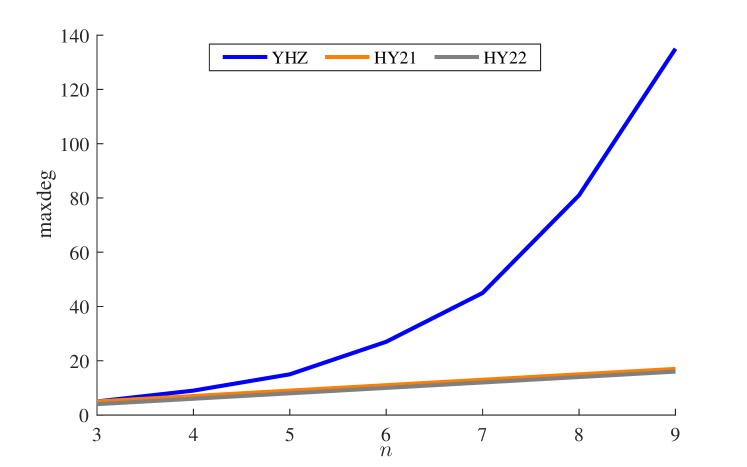
Figure 1: An illustration on the changes of maximal degrees of polynomials in the conditions generated with the three methods along with the degree $n$

Hoon Hong’s work was supported by National Science Foundations of USA (Grant Nos: 2212461 and 1813340). Jing Yang’s work was supported by National Natural Science Foundation of China (Grant Nos.: 12261010 and 11801101).

References

- [1] Basu S, Pollack R, Roy M-F. Algorithms in real algebraic geometry. Springer-Verlag, Berlin-Heidelberg, 2006
- [2] Bóna M. A Walk Through Combinatorics: An Introduction to Enumeration and Graph Theory (4th edition). World Scientific Publishing, 2016
- [3] Brown W, Traub J. On Euclid’s algorithm and the theory of subresultants. Journal of the Association for Computing Machinery, 1971, 18:505–514
- [4] Collins G. Subresultants and reduced polynomial remainder sequences. Journal of the Association for Computing Machinery, 1967, 14:128–142
- [5] González-Vega L, Recio T, Lombardi H, et al. Sturm-Habicht Sequences, Determinants and real roots of univariate polynomials. In Quantifier Elimination and Cylindrical Algebraic Decomposition. Texts and Monographs in Symbolic Computation (A Series of the Research Institute for Symbolic Computation, Johannes-Kepler-University, Linz, Austria). Springer, 1998, 300–316
- [6] Hong H, Yang J. A condition for multiplicity structure of univariate polynomials. arXiv:2001.02388, 2020
- [7] Hong H, Yang J. A condition for multiplicity structure of univariate polynomials. Journal of Symbolic Computation, 2021, 104:523–538
- [8] Liang S, Jeffrey D J. An algorithm for computing the complete root classification of a parametric polynomial. In Calmet J, Ida T, Wang D, eds. Proceedings of the Artificial Intelligence and Symbolic Computation (AISC 2006). Lecture Notes in Computer Science, vol 4120. Springer Berlin Heidelberg, 2006, 116–130
- [9] Liang S, Jeffrey D J, Maza M M. The complete root classification of a parametric polynomial on an interval. In Proceedings of the Twenty-first International Symposium on Symbolic and Algebraic Computation (ISSAC’08). New York: ACM, 2008, 189–196
- [10] Liang S, Zhang J. A complete discrimination system for polynomials with complex coefficients and its automatic generation. Science in China Series E: Technological Sciences, 1999, 42:113–128
- [11] Loos R. Generalized polynomial remainder sequences. In Computer Algebra. Computing Supplementa (Computing), vol 4. Springer Vienna, 1983, 115–137
- [12] Stoer J, Bulirsch R. Interpolation. In: Introduction to Numerical Analysis. Texts in Applied Mathematics, vol 12. Springer, New York, 2002, 37–144
- [13] Yang L, Hou X, Zeng Z. A complete discrimination system for polynomials. Science in China (Series E), 1996, 39(6):628–646