Causal Deep Learning

Abstract

We derive a set of causal deep neural networks whose architectures are a consequence of tensor (multilinear) factor analysis. Forward causal questions are addressed with a neural network architecture composed of causal capsules and a tensor transformer. The former estimate a set of latent variables that represent the causal factors, and the latter governs their interaction. Causal capsules and tensor transformers may be implemented using shallow autoencoders, but for a scalable architecture we employ block algebra and derive a deep neural network composed of a hierarchy of autoencoders. An interleaved kernel hierarchy pre-processes the data resulting in a hierarchy of kernel tensor factor models. Inverse causal questions are addressed with a neural network that implements multilinear projection and estimates the causes of effects. As an alternative to aggressive bottleneck dimension reduction or regularized regression that may camouflage an inherently underdetermined inverse problem, we prescribe modeling different aspects of the mechanism of data formation with piecewise tensor models whose multilinear projections are well-defined and produce multiple candidate solutions. Our forward and inverse neural network architectures are suitable for asynchronous parallel computation.

I Introduction

Building upon prior representation learning efforts aimed at disentangling the causal factors of data variation [28][8][92] [72][71], we derive a set of causal deep neural networks that are a consequence of tensor (multilinear) factor analysis. Tensor factor analysis is a transparent framework for modeling a hypothesized multi-causal mechanisms of data formation, computing invariant causal representations, and estimating the effects of interventions [103][100][108][105]. The validity and strength of causal explanations depend on causal model specifications in conjunction with experimental designs for acquiring suitable training data [81].

Unlike conventional statistics and machine learning which model observed data distributions and make predictions about one variable co-observed with another, or perform time series forecasting, causal inference is a hypothesis-driven process, as opposed to a data-driven process, that models the mechanism of data formation and estimates the effects of interventions [78][46][89][103][99]. Inverse causal “inference” estimates the causes of effects given an estimated forward model and constraints on the solution set [32][100][109].

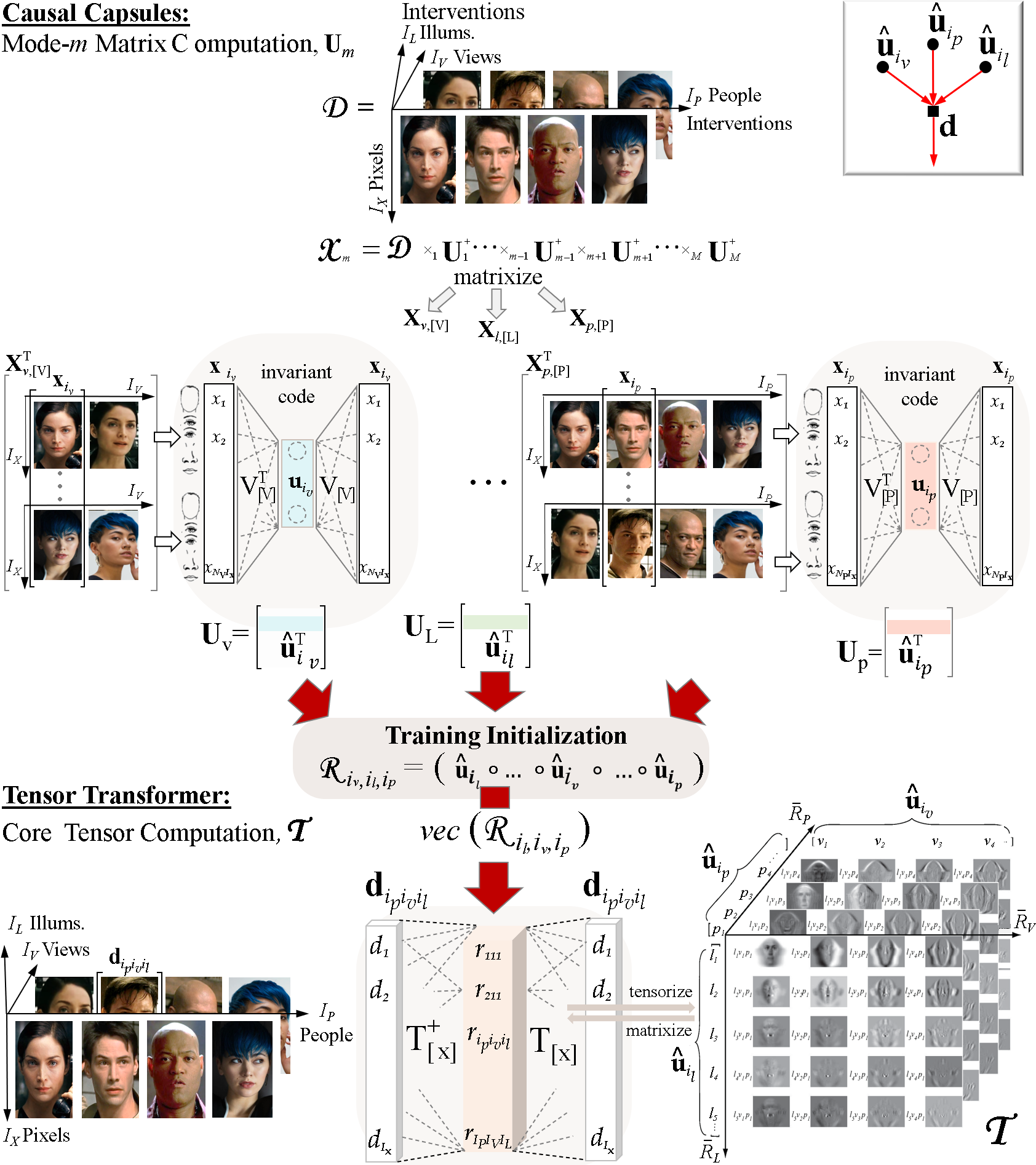
Figure 1: A forward causal neural network is composed of a set of causal capsules and a tensor transformer. Causal capsules estimate the causal factor representations ${\mathbf{U}}_{\mbox{\tiny{m}}}$, and a tensor transformer ${\mathbf{\mathcal{T}}}$ governs their interaction. Causal capsules and tensor transformers can be implemented with a set of shallow autoencoders and tensor autoencoders, respectively. For a scalable architecture, each autoencoder is replaced with a deep neural network composed of a part based hierarchy of autoencoders (Fig. 3f). The above neural network depicts the M-mode SVD [106][105], a parallel multilinear rank decomposition. (In practice, images are vectorized and centered.)

Causal Inference Versus Regression

Neural networks and tensor factorization methods may be causal in nature and perform causal inference, or simply perform regression from which no causal conclusions are drawn. For causal inference, hypothesis-driven experimental design for generating training data [81], and model specifications (Fig. 2) trump algorithmic design and analysis.

I-A Causal Neural Networks

Causal neural networks are composed of causal capsules and tensor transformers (Fig. 1). Causal capsules estimate the latent variables that represent the causal factors of data formation. A tensor transformer governs the interaction of the latent variables. Causal capsules may be implemented as shallow Hebb autoencoders, which perform principal component analysis (PCA) [87][83][82][1][75] (see supplemental Sec VI-A) when the neurons are linear with non-deterministic activation [4][48]. The tensor transformer may be implemented as a tensor autoencoder, a shallow autoencoder whose code is the tensor product of the latent variables.

Causal deep neural networks are composed of stacking Hebb and tensor autoencoders. Each causal capsule or tensor transformer in a shallow causal neural network is replaced by mathematically equivalent deep architectures composed either of a part-based hierarchy of Hebb autoencoders or of a part-based hierarchy of tensor autoencoders. An interleaved hierarchy of kernel functions [86] serves as a pre-processor that warps the data manifold for optimal tensor factor analysis. The resulting deep causal neural network models the mechanism of data formation with a hierarchy of tensor factor models [103][102][99, Sec 4.4] (see Supplemental Section VI-C).

Inverse causal neural networks implement the multilinear projection algorithm to estimate the causes of effects [109][100]. A neural network that addresses an underdetermined inverse problem is characterized by a wide hidden layer. Dimensionality reduction removes noise and nuisance variables [38, 93], and has the added benefit of reducing the widths of hidden layers. However, aggressive bottleneck dimensionality reduction may camouflage an inherently ill-posed problem. Alternatively or in addition to dimensionality reduction and regularized regression, we prescribe modeling different aspects of the data formation process with piecewise tensor (multilinear) models (mixture of experts) whose projections are well-defined [104]. Candidate solutions are gated to yield a unique solution.

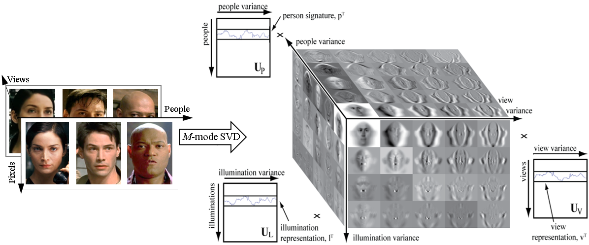
(a)

(b)

Figure 2: Same data, same algorithm, but two different model specifications (problem setups) result in two semantically different decompositions. (a) Causal Inference: The $M$-mode SVD (Algorithm 1) factorizes a “data tensor” of vectorized observations into a set of latent variables that represent the causal factors. (b) Regression: The $M$-mode SVD factorizes a “data tensor” composed of images as a “data matrix” into the image column and row space as well as the normalized PCA coefficients. (Images represent their vectorized versions except in Fig. 2b.)

Input ${\mathbf{\mathcal{D}}}\in\mathbb{C}^{I_{0}\times\dots\times I_{\mbox{\tiny{M}}}}$, dimensions $R_{\mbox{\tiny{0}}},R_{\mbox{\tiny{1}}}\dots R_{\mbox{\tiny{m}}}\dots R_{\mbox{\tiny{M}}}$

1. Initialize ${\mathbf{U}}_{\mbox{\tiny{m}}}\mathrel{\mathop{:}}={\mathbf{I}}$ or random matrix, $0\leq m\leq M$

2. Iterate until convergence

• For $m\mathrel{\mathop{:}}=0,\dots,M$,

  • $\mathbin{\mathchoice{\hbox to5.74991pt{\hfil\raise 0.0pt\hbox{\scalebox{0.75}{\lower 0.0pt\hbox{$\displaystyle\bullet$}}}\hfil}}{\hbox to5.74991pt{\hfil\raise 0.0pt\hbox{\scalebox{0.75}{\lower 0.0pt\hbox{$\textstyle\bullet$}}}\hfil}}{\hbox to4.79156pt{\hfil\raise 0.0pt\hbox{\scalebox{0.75}{\lower 0.0pt\hbox{$\scriptstyle\bullet$}}}\hfil}}{\hbox to4.15268pt{\hfil\raise 0.0pt\hbox{\scalebox{0.75}{\lower 0.0pt\hbox{$\scriptscriptstyle\bullet$}}}\hfil}}}$ ${\mathbf{\mathcal{X}}}\mathrel{\mathop{:}}={\mathbf{\mathcal{D}}}\times_{\mbox{\tiny{0}}}{\mathbf{U}}{}^{\hbox{\tiny{T}}}_{\mbox{\tiny{0}}}\times\dots\times_{\mbox{\tiny{m-1}}}{\mathbf{U}}{}^{\hbox{\tiny{T}}}_{\mbox{\tiny{m-1}}}\times_{\mbox{\tiny{m+1}}}{\mathbf{U}}{}^{\hbox{\tiny{T}}}_{\mbox{\tiny{m+1}}}\dots\times{\mathbf{U}}{}^{\hbox{\tiny{T}}}_{\mbox{\tiny{M}}}$

  • $\mathbin{\mathchoice{\hbox to5.74991pt{\hfil\raise 0.0pt\hbox{\scalebox{0.75}{\lower 0.0pt\hbox{$\displaystyle\bullet$}}}\hfil}}{\hbox to5.74991pt{\hfil\raise 0.0pt\hbox{\scalebox{0.75}{\lower 0.0pt\hbox{$\textstyle\bullet$}}}\hfil}}{\hbox to4.79156pt{\hfil\raise 0.0pt\hbox{\scalebox{0.75}{\lower 0.0pt\hbox{$\scriptstyle\bullet$}}}\hfil}}{\hbox to4.15268pt{\hfil\raise 0.0pt\hbox{\scalebox{0.75}{\lower 0.0pt\hbox{$\scriptscriptstyle\bullet$}}}\hfil}}}$ Set ${\mathbf{U}}_{m}$ to the $\tilde{R}_{m}$ leading left-singular vectors of the SVD of ${{\mathbf{X}}}_{\mbox{\tiny{$[m]$}}}$ or SVD of $[{{\mathbf{X}}}_{\mbox{\tiny{$[m]$}}}{{\mathbf{X}}{}^{\hbox{\tiny{T}}}}_{\mbox{\tiny{$[m]$}}}]$. ^,

3. Set ${\mathbf{\mathcal{Z}}}\mathrel{\mathop{:}}={\mathbf{\mathcal{D}}}\times_{0}{\mathbf{U}}{}^{\hbox{\tiny{T}}}_{\mbox{\tiny{0}}}\dots\times_{\mbox{\tiny{m}}}{\mathbf{U}}{}^{\hbox{\tiny{T}}}_{\mbox{\tiny{m}}}\dots\times_{\mbox{\tiny{M}}}{\mathbf{U}}{}^{\hbox{\tiny{T}}}_{\mbox{\tiny{M}}}\mathrel{\mathop{:}}={\mathbf{\mathcal{X}}}\times{\mathbf{U}}{}^{\hbox{\tiny{T}}}_{\mbox{\tiny{M}}}$

Output mode matrices ${\mathbf{U}}_{0},{\mathbf{U}}_{\mbox{\tiny{1}}},\dots,{\mathbf{U}}_{\mbox{\tiny{M}}}$ and core tensor ${\mathbf{\mathcal{Z}}}$.  

Algorithm 1 $M$-mode SVD (parallel computation)[106, 105]

Input the data tensor ${\mathbf{\mathcal{D}}}\in\mathbb{C}^{I_{0}\times\dots\times I_{M}}$, where mode $m=0$ is the measurement mode, and the desired ranks are $\tilde{R}_{1},\dots,\tilde{R}_{M}$. Initialize ${\mathbf{C}}_{\mbox{\tiny{m}}}={\mathbf{I}}$ or random matrix, $\forall$ $0\leq m\leq M$

Iterate until convergence.

1. For $m\mathrel{\mathop{:}}=1,\dots,M$

   1. Set ${\mathbf{\mathcal{X}}}_{\mbox{\tiny{m}}}\mathrel{\mathop{:}}={\mathbf{\mathcal{D}}}\times_{1}{\mathbf{C}}_{1}^{+}\dots\times_{m-1}{\mathbf{C}}_{m-1}^{+}\times_{m+1}{\mathbf{C}}_{m+1}^{+}\dots\times_{M}{\mathbf{C}}_{M}^{+}.$

   2. Compute the elements of the mode-$m$ covariance matrix, for $j,k\mathrel{\mathop{:}}=1,\dots,I_{m}$:

      $$\hskip 18.06749pt\left[{{\mathbf{X}}}_{\mbox{\tiny{$[m]$}}}{{\mathbf{X}}}_{\mbox{\tiny{$[m]$}}}{}^{\hbox{\tiny{T}}}\right]_{\mbox{\tiny{jk}}}\hskip-1.8063pt\mathrel{\mathop{:}}=\sum_{i_{1}=1}^{I_{1}}...\hskip-3.61371pt\sum_{i_{\mbox{\tiny{m-1}}}=1}^{I_{m-1}}~{}\sum_{i_{\mbox{\tiny{m+1}}}=1}^{I_{\mbox{\tiny{m+1}}}}...\sum_{i_{\mbox{\tiny{M=1}}}}^{I_{M}}\hskip-1.4457ptK({\mathbf{x}}_{i_{\mbox{\tiny{1}}}...i_{\mbox{\tiny{m-1}}}\,j\,i_{\mbox{\tiny{m+1}}}...i_{\mbox{\tiny{M}}}},{\mathbf{x}}_{i_{\mbox{\tiny{1}}}...i_{\mbox{\tiny{m-1}}}\,k\,i_{\mbox{\tiny{m+1}}}...i_{\mbox{\tiny{M}}}}).$$ (1)

   3. $\begin{cases}\text{\sl For K-MPCA:}&\text{Set ${\mathbf{C}}_{\mbox{\tiny{m}}}\mathrel{\mathop{:}}={\mathbf{U}}$ to the left matrix of the SVD, of $\left[{{\mathbf{X}}}_{\mbox{\tiny{$[m]$}}}{{\mathbf{X}}}_{\mbox{\tiny{$[m]$}}}{}^{\hbox{\tiny{T}}}\right]={\mathbf{U}}_{\mbox{\tiny{m}}}{\mathbf{\Sigma}}^{2}{\mathbf{U}}{}^{\hbox{\tiny{T}}}_{\mbox{\tiny{m}}}$ from (\ref{eq:kernelized subspace})}\\[-3.0pt] &\text{Truncate to $\tilde{R}_{m}$ columns ${\mathbf{U}}_{\mbox{\tiny{m}}}\in\mathbb{C}^{I_{m}\times\tilde{R}_{m}}$.}\\[4.0pt] \text{\sl For K-MICA:}&\text{Set ${\mathbf{C}}_{\mbox{\tiny{m}}}\mathrel{\mathop{:}}={\mathbf{U}}_{\mbox{\tiny{m}}}{\mathbf{W}}^{-1\lower 2.0pt\hbox{\hskip-2.0pt\hbox{\tiny${}$}}}_{\mbox{\tiny{m}}}$. The additional invertible matrix ${\mathbf{W}}_{\mbox{\tiny{m}}}$ may be computed based on negentropy, }\\ &\text{mutual information, or higher-order cumulants~{}\cite[cite]{[\@@bibref{}{Vasilescu05}{}{}]}. }\\ &\text{The initial SVD of $\left[{{\mathbf{X}}}_{\mbox{\tiny{$[m]$}}}{{\mathbf{X}}}_{\mbox{\tiny{$[m]$}}}\right]{}^{\hbox{\tiny{T}}}$ (\ref{eq:kernelized subspace}) truncates the subspace to $\tilde{R}_{m}$.}\end{cases}$

2. Set ${\mathbf{\mathcal{B}}}\mathrel{\mathop{:}}={\mathbf{\mathcal{X}}}_{\mbox{\tiny{M}}}\times_{M}{\mathbf{C}}_{M}^{+}$. For K-MPCA, ${\mathbf{C}}^{+\lower 2.0pt\hbox{\hskip-2.0pt\mbox{\tiny${}$}}}_{\mbox{\tiny{M}}}={\mathbf{C}}{}^{\hbox{\tiny{T}}}_{\mbox{\tiny{M}}}.$

Output the converged extended core tensor ${\mathbf{\mathcal{T}}}\in\mathbb{C}^{I_{0}\times\tilde{R}_{1}\times\dots\times\tilde{R}_{M}}$ and causal factor mode matrices ${\mathbf{C}}_{1},\dots,{\mathbf{C}}_{M}$.

Algorithm 2 Kernel Tensor Factor Analysis [99, Sec 4.4][108]
Kernel Multilinear Independent Component Analysis (K-MICA) and Kernel Principal Component Analysis (K-MPCA).

Linear kernel: $K({\mathbf{u}},{\mathbf{v}})={\mathbf{u}}{}^{\hbox{\tiny{T}}}{\mathbf{v}}={\mathbf{u}}\cdot{\mathbf{v}}$ Polynomial kernel of degree $d$: $K({\mathbf{u}},{\mathbf{v}})=({\mathbf{u}}{}^{\hbox{\tiny{T}}}{\mathbf{v}})^{d}$ Polynomial kernel up to degree $d$: $K({\mathbf{u}},{\mathbf{v}})=({\mathbf{u}}{}^{\hbox{\tiny{T}}}{\mathbf{v}}+1)^{d}$ Sigmoidal kernel: $K({\mathbf{u}},{\mathbf{v}})=\tanh(\alpha\,{\mathbf{u}}{}^{\hbox{\tiny{T}}}{\mathbf{v}}+\beta)$ Gaussian (radial basis function (RBF)) kernel: $K({\mathbf{u}},{\mathbf{v}})=\exp\left(-{\|{\mathbf{u}}-{\mathbf{v}}\|^{2}\over 2\sigma^{2}}\right)$ TABLE I: Common kernel functions. Kernel functions are symmetric, positive semi-definite functions corresponding to symmetric, positive semi-definite Gram matrices. The linear kernel does not modify or warp the feature space.

II Forward Causal Question: “What if?”

Forward causal inference is a hypothesis-driven process that addresses the “what if” question. Causal hypotheses drive both the experimental design for generating training data and the causal model specification.

Training Data: For modeling the unit level effects of causes, the training data is generated by combinatorially varying each causal factor while holding the other factors fixed. The best causal evidence comes from randomized experimental studies. When physical, or statistical experiments for generating training data are unethical or infeasible, experiments may be approximated with carefully designed observational studies [81], such as natural experiments [2][16][47]. The certainty of causal conclusions are dependent on the type of evidence employed.

Models: Within the tensor mathematical framework (Supplemental Section VI-B) a “data tensor,” ${\mathbf{\mathcal{D}}}\in\mathbb{C}^{I_{\mbox{\tiny{0}}}\times I_{\mbox{\tiny{1}}}\dots\times I_{\mbox{\tiny{m}}}\dots\times I_{\mbox{\tiny{M}}}}$, contains a collection of vectorized and centered observations, ${\mathbf{d}}_{i_{\mbox{\tiny{1}}}\dots i_{\mbox{\tiny{m}}}\dots i_{\mbox{\tiny{M}}}}\in\mathbb{C}^{I_{\mbox{\tiny{0}}}}$ that are the result of $M$ causal factors. Causal factor $m$ ($1\leq m\leq M$) takes one of $I_{m}$ values that are indexed by $i_{m}$, $1\leq i_{m}\leq I_{m}$. An observation and a data tensor are modeled by a multilinear equation with multimode latent variables:

$${\mathbf{\mathcal{D}}} = {\mathbf{\mathcal{T}}}\times_{\mbox{\tiny{1}}}{\mathbf{U}}_{\mbox{\tiny{1}}}\dots\times{\mathbf{U}}_{\mbox{\tiny{m}}}\times_{\mbox{\tiny{M}}}{\mathbf{U}}_{\mbox{\tiny{M}}}+{\mathbf{\mathcal{E}}},$$ (2)

$${\mathbf{d}}_{i_{\mbox{\tiny{1}}},\dots,i_{\mbox{\tiny{M}}}} = {\mathbf{\mathcal{T}}}\times_{\mbox{\tiny{1}}}({\mathbf{\hat{u}}}{}^{\hbox{\tiny{T}}}_{i_{\mbox{\tiny{1}}}}+\epsilon{}^{\hbox{\tiny{T}}}_{i_{\mbox{\tiny{1}}}})\dots\times_{\mbox{\tiny{M}}}({\mathbf{\hat{u}}}{}^{\hbox{\tiny{T}}}_{i_{\mbox{\tiny{M}}}}+\epsilon{}^{\hbox{\tiny{T}}}_{i_{\mbox{\tiny{M}}}})+\xi_{i_{\mbox{\tiny{1}}},\dots,i_{\mbox{\tiny{M}}}},$$

where ${\mathbf{\mathcal{T}}}$ is the extended core that contains the basis vectors and governs the interaction between the latent variables ${\mathbf{\hat{u}}}{}^{\hbox{\tiny{T}}}_{i_{\mbox{\tiny{m}}}}$ (row $i$ of ${\mathbf{U}}_{\mbox{\tiny{m}}}$) that represent the causal factors of data formation, ${\mathbf{\bm{\epsilon}}}_{i_{\mbox{\tiny{m}}}}\in{\mathbf{\mathcal{N}}}({\mathbf{0}},{\mathbf{\Sigma}}_{\mbox{\tiny{m}}})$ are disturbances with Gaussian distribution, and $\xi_{i_{\mbox{\tiny{1}}},\dots,i_{\mbox{\tiny{M}}}}$ is a Gaussian measurement error.

Minimizing the cost function

$$L = \|{\mathbf{\mathcal{D}}}-{\mathbf{\mathcal{T}}}\times_{\mbox{\tiny{1}}}{\mathbf{U}}_{\mbox{\tiny{1}}}...\times_{\mbox{\tiny{m}}}{\mathbf{U}}_{\mbox{\tiny{m}}}...\times_{\mbox{\tiny{M}}}{\mathbf{U}}_{\mbox{\tiny{M}}}\|+\sum_{m=1}^{M}\lambda_{\mbox{\tiny{m}}}\|{\mathbf{U}}_{\mbox{\tiny{m}}}{\mathbf{U}}{}^{\hbox{\tiny{T}}}_{\mbox{\tiny{m}}}-{\mathbf{I}}\|\vspace{-.05in}$$

is equivalent to maximum likelihood estimation [27] of the causal factor parameters, assuming the data was generated by the model with additive Gaussian noise. The optimal mode matrices ${\mathbf{U}}_{\mbox{\tiny{m}}}$ are computed by employing a set of $M$ alternating least squares optimizations.

$$L_{\mbox{\tiny{m}}} = \|{\mathbf{\mathcal{X}}}_{\mbox{\tiny{m}}}-{\mathbf{\mathcal{T}}}\times_{\mbox{\tiny{m}}}{\mathbf{U}}_{\mbox{\tiny{m}}}\|+\lambda_{\mbox{\tiny{m}}}\|{\mathbf{U}}{}^{\hbox{\tiny{T}}}_{\mbox{\tiny{m}}}\times{\mathbf{U}}_{\mbox{\tiny{m}}}-{\mathbf{I}}\|,\hskip 3.61371pt\mbox{where}$$

$${\mathbf{\mathcal{X}}}_{\mbox{\tiny{m}}} \mathrel{\mathop{:}}= {{\mathbf{\mathcal{D}}}\times_{\mbox{\tiny{1}}}...\times_{\mbox{\tiny{m-1}}}{\mathbf{U}}{}^{\hbox{\tiny{T}}}_{\mbox{\tiny{m-1}}}\times_{\mbox{\tiny{m+1}}}{\mathbf{U}}{}^{\hbox{\tiny{T}}}_{\mbox{\tiny{m+1}}}...\times_{\mbox{\tiny{M}}}{\mathbf{U}}{}^{\hbox{\tiny{T}}}_{\mbox{\tiny{M}}}}\hskip 1.8063pt\mbox{- parallel}$$ (3)

$$= {\mathbf{\mathcal{X}}}_{\mbox{\tiny{m}}}\mbox{\small$(t-1)$}\times_{\mbox{\tiny{n}}}{\mathbf{U}}{}^{\hbox{\tiny{T}}}_{\mbox{\tiny{n}}}\mbox{\small$(t)$}{\mathbf{U}}_{\mbox{\tiny{n}}}\mbox{\small$(t-1)$},\hskip 1.8063pt\forall\mbox{\small$n\neq m$},\hskip 1.4457pt\mbox{- asynchronous~{}~{}}$$ (4)

$$= ({\mathbf{\mathcal{X}}}_{\mbox{\tiny{m-1}}}\times_{\mbox{\tiny{m-1}}}{\mathbf{U}}{}^{\hbox{\tiny{T}}}_{\mbox{\tiny{m-1}}})\times_{\mbox{\tiny{m}}}{\mathbf{U}}_{\mbox{\tiny{m}}}={\mathbf{\mathcal{T}}}\times_{\mbox{\tiny{m}}}{\mathbf{U}}_{\mbox{\tiny{m}}}\hskip 9.03374pt\mbox{- sequential}$$ (5)

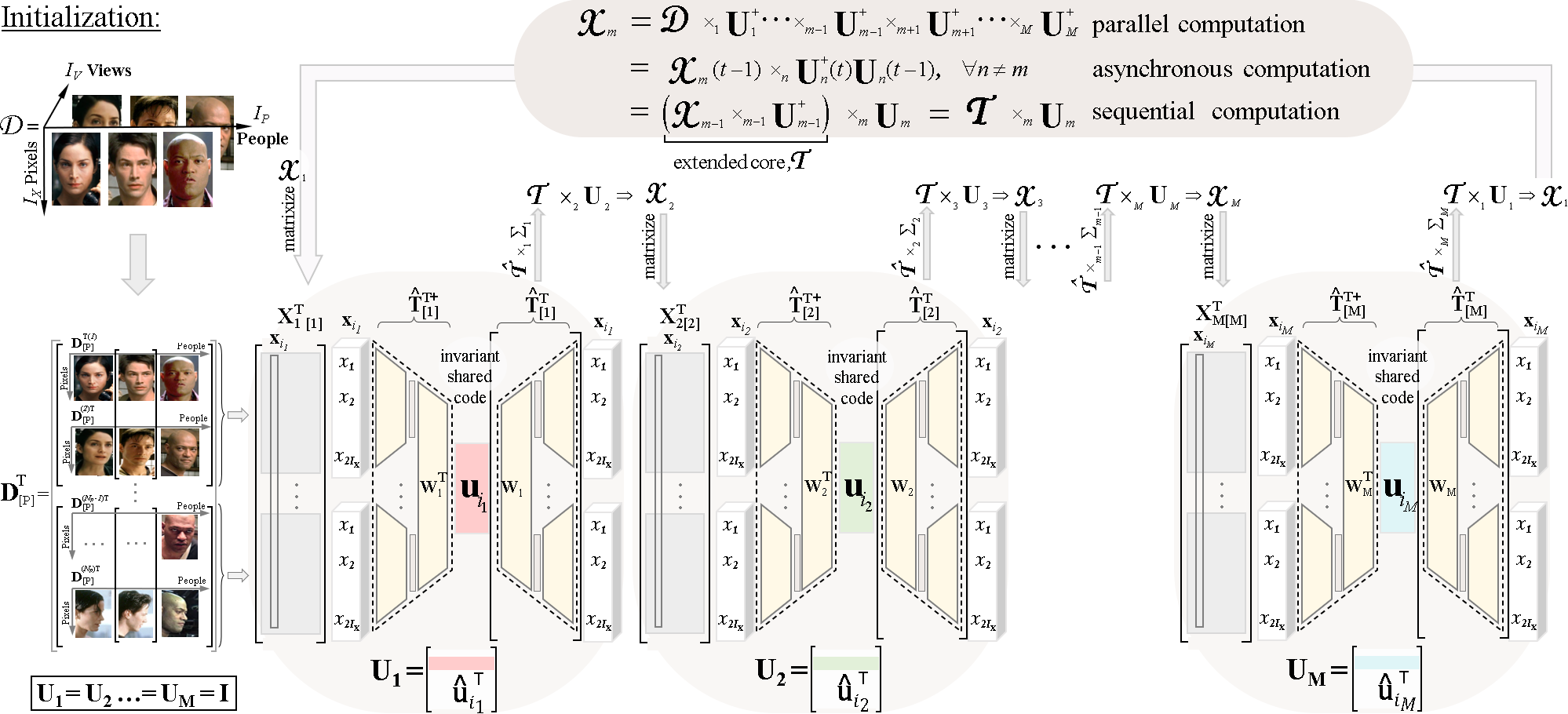
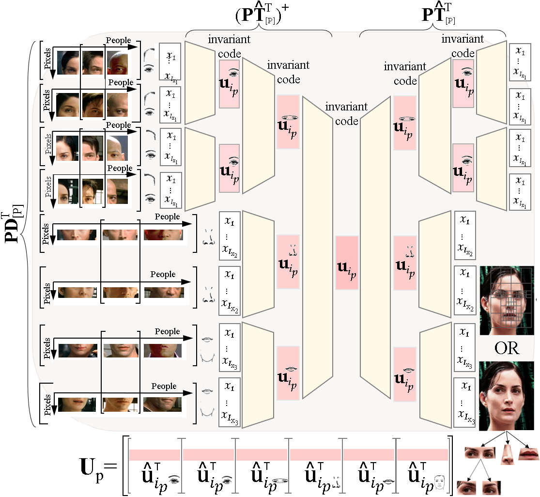
(a)
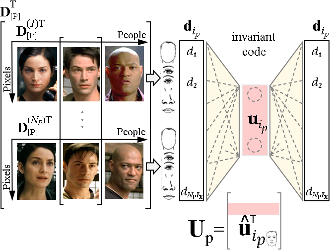
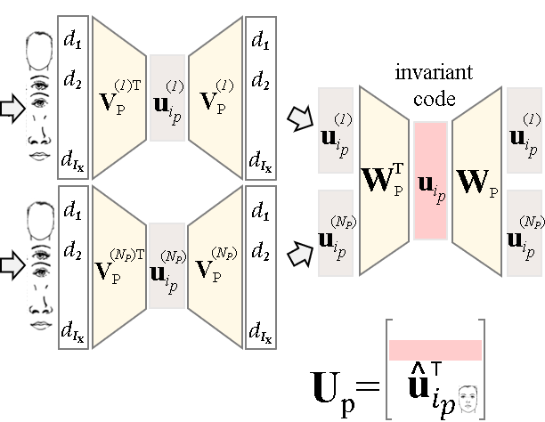
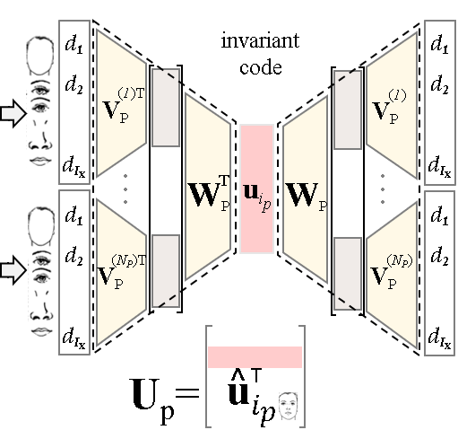
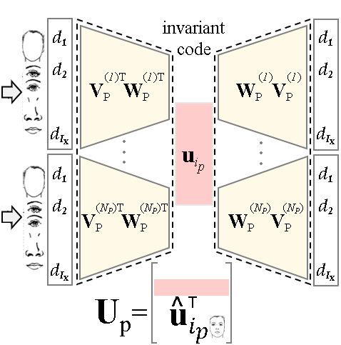
                     (b)                   (c) (d) (e)                                                  (f)                                                                  (g)

Figure 3: Deep neural network. Subfigures (a-e) depict (21–29) [99, pg.38-40]. (a) The mode matrix computation ${\mathbf{U}}_{\mbox{\tiny{m}}}$ is a constrained cluster-based PCA that is rewritten in terms of block SVDs. Matrixizing may be viewed as a concatenation of “cluster” data. The matrix ${\mathbf{W}}$ transforms the basis matrix ${\mathbf{U}}^{(n)}_{\mbox{\tiny{0}}}$ such that the causal factor representation ${\mathbf{U}}_{\mbox{\tiny{m}}}$ is the same regardless of cluster membership. (b) Mode matrix ${\mathbf{U}}_{\mbox{\tiny{m}}}$ computation using a single autoencoder-decoder. (c) Mode matrix computation as a hierarchy of autoencoder-decoders, (d) Mode matrix computation written as a deep learning model (e) Concurrent-autoencoders; i.e., constrained cluster-based autoencoders. (f) Forward causal model with a set of capsules implemented by deep neural networks. For parallel computation, we break the chain links and shuttle causal information between capsules. (g) Each capsule in (f) may be replaced with a part-based deep neural network by permuting the rows in ${{\mathbf{D}}{}^{\hbox{\tiny{T}}}}_{\mbox{\tiny{$[m]$}}}$, and segmenting them based on adaptive subdivision [96]. The capsules are efficiently trained with a part-based hierarchy of autoencoders (Fig. 4).

The $M$-mode SVD [105] (Algorithm 1) minimizes $M$ alternating least squares in closed form by employing $M$ different SVDs. It is suitable for parallel computation, but can be performed asynchronously or sequentially by employing (4) and (5), respectively. The core tensor ${\mathbf{\mathcal{T}}}$ is computed by multiplying the data tensor with the inverse mode matrices, ${\mathbf{\mathcal{T}}}={\mathbf{\mathcal{D}}}\times_{\mbox{\tiny{1}}}{\mathbf{U}}{}^{\hbox{\tiny{T}}}_{\mbox{\tiny{1}}}\dots\times_{\mbox{\tiny{m}}}{\mathbf{U}}{}^{\hbox{\tiny{T}}}_{\mbox{\tiny{m}}}\dots\times_{\mbox{\tiny{M}}}{\mathbf{U}}{}^{\hbox{\tiny{T}}}_{\mbox{\tiny{M}}}$, or more efficiently as ${\mathbf{\mathcal{T}}}={\mathbf{\mathcal{X}}}_{\mbox{\tiny{m}}}\times{\mathbf{U}}{}^{\hbox{\tiny{T}}}_{\mbox{\tiny{m}}}$.

II-A Kernel Tensor Factor Analysis:

When data ${\mathbf{\mathcal{D}}}$ are a combination of non-linear independent causal factors ${\mathbf{C}}$,

$${\mathbf{\mathcal{D}}} = {\mathbf{\mathcal{B}}}\times_{\mbox{\tiny{1}}}\phi({\mathbf{C}}_{\mbox{\tiny{1}}})\dots\times\phi({\mathbf{C}}_{\mbox{\tiny{m}}})\dots\times_{\mbox{\tiny{M}}}\phi({\mathbf{C}}_{\mbox{\tiny{M}}})+{\mathbf{\mathcal{E}}}\hskip 3.61371pt$$ (6)

$${\mathbf{C}}_{\mbox{\tiny{m}}} = {\mathbf{U}}_{\mbox{\tiny{m}}}{\mathbf{W}}^{-1\lower 2.0pt\hbox{\hskip-2.0pt\hbox{\tiny${}$}}}{}+{\mathbf{E}}_{\mbox{\tiny{m}}},$$

kernel multilinear independent component analysis (K-MICA) [99, Ch 4.4] models the mechanism of data formation. K-MICA employs the “kernel trick” [85][110] as a pre-processing step which makes the data suitable for multilinear independent component analysis [108] (Algorithm 2), where the additional rotation matrix ${\mathbf{W}}_{\mbox{\tiny{m}}}$ may be computed based on negentropy, mutual information, or higher-order cumulants. K-MICA is a tensor generalization of the kernel PCA [86] and kernel ICA [3][114].

To accomplish this analysis, recall that the computation of covariance matrix ${{\mathbf{D}}}_{\mbox{\tiny{$[m]$}}}{{\mathbf{D}}}_{\mbox{\tiny{$[m]$}}}{}^{\hbox{\tiny{T}}}$ involves inner products ${\mathbf{d}}{}^{\hbox{\tiny{T}}}_{i_{\mbox{\tiny{1}}}\dots i_{\mbox{\tiny{m-1}}}\,j\,i_{\mbox{\tiny{m+1}}}\dots i_{\mbox{\tiny{M}}}}{\mathbf{d}}_{i_{\mbox{\tiny{2}}}\dots i_{\mbox{\tiny{m-1}}}\,k\,i_{\mbox{\tiny{m+1}}}\dots i_{\mbox{\tiny{M}}}}$ between pairs of data points in the data tensor ${\mathbf{\mathcal{D}}}$ associated with causal factor mode $m$, for $m=1,\dots,M$ (Step 2.2 in Algorithm 1). We replace the inner products with a generalized distance measure between images, $K({\mathbf{d}}_{i_{1}\dots i_{m-1}\,j\,i_{m+1}\dots i_{\mbox{\tiny{M}}}},{\mathbf{d}}_{i_{2}\dots i_{m-1}\,k\,i_{m+1}\dots i_{\mbox{\tiny{M}}}})$, where $K(\cdot,\cdot)$ is a suitable kernel function (Table I) that corresponds to an inner product in some expanded feature space. This generalization naturally leads us to a Kernel Multilinear PCA (K-MPCA) Algorithm, where the covariance computation is replaced by

$$\left[{{\mathbf{D}}}_{\mbox{\tiny{$[m]$}}}{{\mathbf{D}}}_{\mbox{\tiny{$[m]$}}}{}^{\hbox{\tiny{T}}}\right]_{jk} \mathrel{\mathop{:}}= \sum_{i_{1}=1}^{I_{1}}\cdots\sum_{i_{m-1}=1}^{I_{m-1}}~{}\sum_{i_{m+1}=1}^{I_{m+1}}\cdots\sum_{i_{\mbox{\tiny{M}}}=1}^{I_{\mbox{\tiny{M}}}}$$

$$K({\mathbf{d}}_{i_{1}\dots i_{m-1}\,j\,i_{m+1}\dots i_{\mbox{\tiny{M}}}},{\mathbf{d}}_{i_{1}\dots i_{m-1}\,k\,i_{m+1}\dots i_{\mbox{\tiny{M}}}}).$$

When a causal factor is a combination of multiple independent sources that are causal in nature, we employ a rotation matrix ${\mathbf{W}}$ to identify them. The rotation matrix is computed by employing either mutual information, negentropy, or higher-order cumulants [23][6][45][5]. A Kernel Multilinear ICA (K-MICA) Algorithm is a kernel generalization of the multilinear independent component analysis (MICA) algorithm [108]. Algorithm 2 simultaneously specifies both K-MPCA and K-MICA algorithms. A scalable tensor factor analysis represents an observation as a hierarchy of parts and wholes [103][102].

III Neural network architecture

Causal neural networks (Fig. 1) parallel the functionality and composition of tensor factor analysis models. Causal neural networks are composed of a set of causal capsules and a tensor transformer. The capsules compute the latent variables, ${\mathbf{U}}_{\mbox{\tiny{m}}}$, that represent the causal factors. The tensor transformer, ${\mathbf{\mathcal{T}}}$, encodes the interaction between the causal factors.

Tensor factor analysis models are transformed into causal neural networks by using Hebb autoencoders and tensor autoencoders as building blocks. The M-mode SVD (Algorithm 1) is transformed into a causal neural network (Fig. 1) by replacing every SVD step with gradient descent optimization, which is outsourced to a Hebb autoencoder (Supplemental Section VI-A). For effectiveness, we employ stochastic gradient descent [12][80]. The extended core tensor ${{\mathbf{T}}}_{\mbox{\tiny{$[0]$}}}$ is computed by defining and employing a tensor autoencoder, an autoencoder whose code is initialized to the tensor product of the causal factor representations, ${{\mathbf{D}}}_{\mbox{\tiny{$[0]$}}}={{\mathbf{T}}}_{\mbox{\tiny{$[0]$}}}({\mathbf{U}}_{i_{\mbox{\tiny{M}}}}\otimes\dots\otimes{\mathbf{U}}_{i_{\mbox{\tiny{m}}}}\dots\otimes{\mathbf{U}}_{i_{\mbox{\tiny{1}}}}){}^{\hbox{\tiny{T}}}.$ To address a set of arbitrarily non-linear causal factors, each autoencoder employs kernel activation functions (Table I).

III-A Causal Deep Networks and Scalable Tensor Factor Analysis:

For a scalable architecture, we leverage the properties of block algebra. Shallow autoencoders are replaced with either a mathematically equivalent deep neural network that requires end-to-end training, a part-based hierarchy of autoencoders [103], or a set of concurrent autoencoders (Fig. 3).

For example, the orthonormal subspace of a data matrix, ${\mathbf{D}}\in\mathbb{C}^{I_{\mbox{\tiny{0}}}\times I_{\mbox{\tiny{1}}}}$ that has $I_{\mbox{\tiny{0}}}$ measurements and $I_{\mbox{\tiny{1}}}$ observations may be computed by recursively subdividing the data and analyzing the data blocks,

$${\mathbf{D}} = \left[\begin{array}[]{cc}{\mathbf{D}}_{\mbox{\tiny{A}}}\\ {\mathbf{D}}_{\mbox{\tiny{B}}}\end{array}\right]=\left[\begin{array}[]{c}{\mathbf{U}}_{\mbox{\tiny{A}}}{\mathbf{S}}_{\mbox{\tiny{A}}}{\mathbf{V}}{}^{\hbox{\tiny{T}}}_{\mbox{\tiny{A}}}\\ {\mathbf{U}}_{\mbox{\tiny{B}}}{\mathbf{S}}_{\mbox{\tiny{B}}}{\mathbf{V}}{}^{\hbox{\tiny{T}}}_{\mbox{\tiny{B}}}\end{array}\right]=\left[\begin{array}[]{cc}{\mathbf{U}}_{\mbox{\tiny{A}}}&{\mathbf{0}}\\ {\mathbf{0}}&{\mathbf{U}}_{\mbox{\tiny{B}}}\end{array}\right]\underbrace{\left[\begin{array}[]{c}{\mathbf{S}}_{\mbox{\tiny{A}}}{\mathbf{V}}{}^{\hbox{\tiny{T}}}_{\mbox{\tiny{A}}}\\ {\mathbf{S}}_{\mbox{\tiny{B}}}{\mathbf{V}}{}^{\hbox{\tiny{T}}}_{\mbox{\tiny{B}}}\end{array}\right]}_{\mbox{SVD}}=$$ (15)

$$= \left[\begin{array}[]{cc}{\mathbf{U}}_{\mbox{\tiny{A}}}&{\mathbf{0}}\\ {\mathbf{0}}&{\mathbf{U}}_{\mbox{\tiny{B}}}\end{array}\right]{\mathbf{W}}{\mathbf{\Sigma}}{\mathbf{V}}{}^{\hbox{\tiny{T}}}=\left[\begin{array}[]{c}{\mathbf{U}}_{\mbox{\tiny{A}}}{\mathbf{W}}_{\mbox{\tiny{A}}}\\ {\mathbf{U}}_{\mbox{\tiny{B}}}{\mathbf{W}}_{\mbox{\tiny{B}}}\end{array}\right]{\mathbf{\Sigma}}{\mathbf{V}}{}^{\hbox{\tiny{T}}}={\mathbf{U}}{\mathbf{\Sigma}}{\mathbf{V}}{}^{\hbox{\tiny{T}}},$$ (20)

where ${\mathbf{W}}$ is a rotation matrix that transforms the basis matrices, ${\mathbf{U}}_{\mbox{\tiny{A}}}$ and ${\mathbf{U}}_{\mbox{\tiny{B}}}$, spanning the data blocks, ${\mathbf{D}}_{\mbox{\tiny{A}}}$ and ${\mathbf{D}}_{\mbox{\tiny{B}}}$, such that their observations have the same representations. This approach can be applied bottom up to a recursively partioned data matrix. The above equalities provide mathematical justification for greedy layer training of deep neural networks [9](Fig. 3a-e).

Computing the mode matrices ${\mathbf{U}}_{\mbox{\tiny{m}}}$ of a tensor model may be viewed as equivalent to computing a set of mutually constrained, cluster-based PCAs [99, pg.38-40] (Fig. 3a). When dealing with data that can be separated into clusters, the standard machine learning approach is to compute a separate PCA. When data from different clusters are generated by the same underlying process (e.g., facial images of the same people under different viewing conditions), the underlying data can be concatenated in the measurement mode and the common causal factor can be modeled by one PCA.

Thus, we define a constrained, cluster-based PCA as the computation of a set of PCA basis vectors that are rotated such that the latent representation is constrained to be the invariant of the cluster membership.

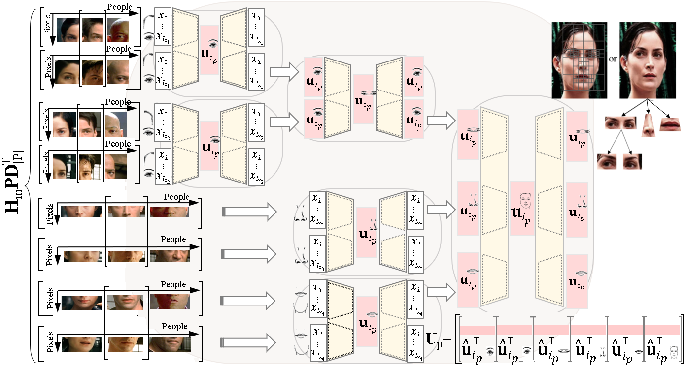
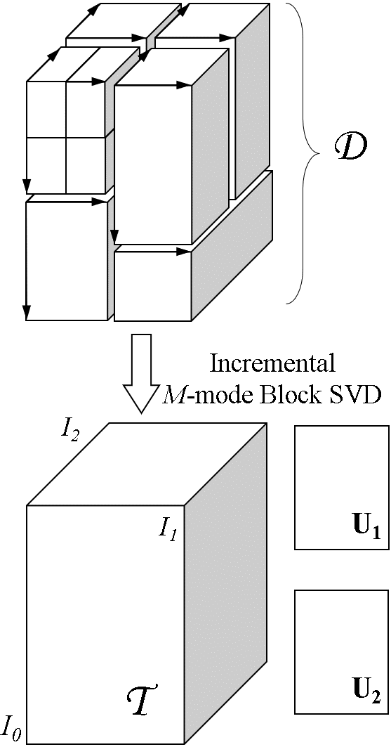
(a)	(b)

Figure 4: (a) Causal capsules may be implemented with a part-based hierarchy of autoencoders. The dataset is permuted by ${\mathbf{P}}$, filtered and segmented by ${\mathbf{H}}_{\mbox{\tiny{m}}}$ that is mode dependent. Subdivision into parts can be determined with adaptive subdivision [96].(b) Implementing the capsules with a part-based hierarchy of autoencoders is equivalent to performing Incremental M-mode Block SVD[103, Sec IV][98].

In the context of our multifactor data analysis, we define a cluster as a set of observations for which all factors are fixed but one. For every tensor mode, there are $N_{\mbox{\tiny{m}}}=I_{1}I_{2}\dots I_{m-1}I_{m+1}\dots I_{\mbox{\tiny{M}}}$ possible clusters and the data in each cluster varies with the same causal mode. The constrained, cluster-based PCA concatenates the clusters in the measurement mode and analyzes the data with a linear model, such as PCA or ICA [5, 23, 26].

To see this, let ${\mathbf{\mathcal{D}}}_{i_{1}\dots i_{m-1}i_{m+1}\dots i_{\mbox{\tiny{M}}}}\in\mathbb{C}^{I_{0}\times 1\times 1\dots\times 1\times I_{\mbox{\tiny{m}}}\times 1\dots\times 1}$ denote a subtensor of ${\mathbf{\mathcal{D}}}$ that is obtained by fixing all causal factor modes but mode $m$ and mode 0 (the measurement mode). Matrixizing this subtensor in the measurement mode we obtain ${{\mathbf{D}}_{i_{1}\dots i_{m-1}i_{m+1}\dots i_{\mbox{\tiny{M}}}}}_{\mbox{\tiny{$[0]$}}}\in\mathbb{C}^{I_{0}\times I_{\mbox{\tiny{m}}}}$. This data matrix comprises a cluster of data obtained by varying causal factor $m$, to which one can traditionally apply PCA. Since there are $N_{\mbox{\tiny{m}}}=I_{1}I_{2}\dots I_{m-1}I_{m+1}\dots I_{\mbox{\tiny{M}}}$ possible clusters that share the same underlying space associated with factor $m$, the data can be concatenated and PCA performed in order to extract the same representation for factor $m$ regardless of the cluster. Now, consider the MPCA computation of mode matrix ${\mathbf{U}}_{\mbox{\tiny{m}}}$ (Fig. 3a), which can be written in terms of matrixized subtensors as

$${{\mathbf{D}}_{\mbox{\tiny{m}}}}=\left[\begin{array}[]{c}{{{\mathbf{D}}_{1\dots 11\dots 1}}_{\mbox{\tiny{$[m]$}}}}{}^{\hbox{\tiny{T}}}\\ {\tiny\vdots}\\ {{\mathbf{D}}_{I_{1}\dots 11\dots 1}}_{\mbox{\tiny{$[m]$}}}{}^{\hbox{\tiny{T}}}\\ {\tiny\vdots}\\ {{{\mathbf{D}}_{I_{1}\dots I_{m-1}I_{m+1}\dots I_{\mbox{\tiny{M}}}}}_{\mbox{\tiny{$[m]$}}}}{}^{\hbox{\tiny{T}}}\end{array}\right]^{{}^{\hbox{\tiny{T}}}}={\mathbf{U}}_{\mbox{\tiny{m}}}{\mathbf{\Sigma}}_{\mbox{\tiny{m}}}{\mathbf{V}}_{\mbox{\tiny{m}}}{}^{\hbox{\tiny{T}}}.$$ (21)

This is equivalent to computing a set of $N_{\mbox{\tiny{m}}}=I_{1}I_{2}\dots I_{m-1}I_{m+1}\dots I_{\mbox{\tiny{M}}}$ cluster-based PCAs concurrently by combining them into a single statistical model and representing the underlying causal factor $m$ common to the clusters. Thus, rather than computing a separate linear PCA model for each cluster, MPCA concatenates the clusters into a single statistical model and computes a representation (coefficient vector) for mode $m$ that is invariant relative to the other causal factor modes $1,...,(m-1),(m+1),...,M$. Thus, MPCA is a multilinear, constrained, cluster-based PCA.

Figure 5: An inverse causal neural network is an inverted forward model where the operations are performed in reverse order  [100][109].

To clarify the relationship, let us number each of the matrices ${{\mathbf{D}}_{i_{1}\dots i_{m-1}i_{m+1}\dots i_{\mbox{\tiny{M}}}}}_{\mbox{\tiny{$[m]$}}}={\mathbf{D}}_{\mbox{\tiny{m}}}^{(n)}$ with a parenthetical superscript $1\leq n=1+\sum_{k=1,k\neq m}^{M}(i_{n}-1)\prod_{l=1,l\neq m}^{k-1}I_{l}\leq N_{\mbox{\tiny{m}}}$.

Let each of the cluster SVDs be ${\mathbf{D}}_{\mbox{\tiny{m}}}^{(n)}={\mathbf{U}}_{\mbox{\tiny{m}}}^{(n)}{\mathbf{\Sigma}}_{\mbox{\tiny{m}}}^{(n)}{{\mathbf{V}}_{m}^{(n)}}{}^{\hbox{\tiny{T}}}$, and

$${{\mathbf{D}}}_{\mbox{\tiny{$[m]$}}}\hskip-9.03374pt = \hskip-7.22743pt\underbrace{\left[\hskip-3.61371pt\begin{array}[]{c}{\mathbf{U}}_{\mbox{\tiny{m}}}^{(1)}{\mathbf{\Sigma}}_{\mbox{\tiny{m}}}^{(1)}\dots\mathbf{U}_{\mbox{\tiny{m}}}^{(N_{\mbox{\tiny{M}}})}{\mathbf{\Sigma}}_{\mbox{\tiny{m}}}^{(N_{\mbox{\tiny{m}}})}\end{array}\hskip-3.61371pt\right]}_{\mbox{SVD}}\mathop{\mathrm{diag}}([\hskip-3.61371pt\begin{array}[]{c}{\mathbf{V}}^{(1)}_{\mbox{\tiny{m}}}\dots\mathbf{V}^{(N_{\mbox{\tiny{m}}})}_{\mbox{\tiny{m}}}\end{array}\hskip-3.61371pt]){}^{\hbox{\tiny{T}}}$$ (24)

$$= {\mathbf{U}}_{\mbox{\tiny{m}}}{\mathbf{\Sigma}}_{\mbox{\tiny{m}}}{\mathbf{W}}{}^{\hbox{\tiny{T}}}_{\mbox{\tiny{m}}}\mathop{\mathrm{diag}}([\begin{array}[]{ccc}{\mathbf{V}}_{\mbox{\tiny{m}}}^{(1)}&\dots&{\mathbf{V}}_{\mbox{\tiny{m}}}^{(N_{\mbox{\tiny{m}}})}\end{array}]){}^{\hbox{\tiny{T}}},$$ (26)

$$= {\mathbf{U}}_{\mbox{\tiny{m}}}{\mathbf{\Sigma}}_{\mbox{\tiny{m}}}[\begin{array}[]{ccc}{\mathbf{V}}^{(1)}_{\mbox{\tiny{m}}}{\mathbf{W}}^{(1)}_{\mbox{\tiny{m}}}&\dots&{\mathbf{V}}^{(N_{\mbox{\tiny{m}}})}_{\mbox{\tiny{m}}}{\mathbf{W}}^{(N_{\mbox{\tiny{m}}})}_{\mbox{\tiny{m}}}\end{array}]{}^{\hbox{\tiny{T}}}$$ (28)

$$= {\mathbf{U}}_{\mbox{\tiny{m}}}{\mathbf{\Sigma}}_{\mbox{\tiny{m}}}{\mathbf{V}}_{\mbox{\tiny{m}}}{}^{\hbox{\tiny{T}}},$$ (29)

where $\mathop{\mathrm{diag}}(\cdot)$ denotes a diagonal matrix whose elements are each of the elements of its vector argument. The mode matrix ${\mathbf{V}}^{(n_{\mbox{\tiny{m}}})}_{\mbox{\tiny{m}}}$ is the measurement matrix ${\mathbf{U}}^{(n_{\mbox{\tiny{m}}})}_{\mbox{\tiny{0}}}$ (${\mathbf{U}}^{(n_{\mbox{\tiny{m}}})}_{\mbox{\tiny{x}}}$ when the measurements are image pixels) that contains the eigenvectors spanning the observed data in cluster $n_{\mbox{\tiny{m}}}$, $1\leq n_{\mbox{\tiny{m}}}\leq N_{\mbox{\tiny{m}}}$. MPCA can be thought as computing a rotation matrix, ${\mathbf{W}}_{\mbox{\tiny{m}}}$, that contains a set of blocks ${\mathbf{W}}^{(n)}_{\mbox{\tiny{m}}}$ along the diagonal that transform the PCA cluster eigenvectors ${\mathbf{V}}^{(n_{\mbox{\tiny{m}}})}_{\mbox{\tiny{m}}}$ such that the mode matrix ${\mathbf{U}}_{\mbox{\tiny{m}}}$ is the same regardless of cluster membership (24–29)(Fig 3). The constrained “cluster”-based PCAs may also be implemented with a set of concurrent “cluster”-based PCAs.

Causal factors of object wholes may be computed efficiently from their parts, by applying a permutation matrix ${\mathbf{P}}$ and creating part-based data clusters with a segmentation filter ${\mathbf{H}}_{\mbox{\tiny{m}}}$, where ${\mathbf{\mathcal{D}}}\hskip 3.61371pt\,\times^{\hskip-11.0pt\hbox{\tiny{}T}}_{\mbox{\tiny{m}}}{\mathbf{H}}_{\mbox{\tiny{m}}}{\mathbf{P}}\Leftrightarrow{\mathbf{H}}_{\mbox{\tiny{m}}}{\mathbf{P}}{{{\mathbf{D}}}_{\mbox{\tiny{$[m]$}}}}{}^{\hbox{\tiny{T}}}$, but leaving prior analysis intact (Fig. 3g). A deep neural network can be efficiently trained with a hierarchy of part-based autoencoders (Fig. 4). A computation that employs a part-based hierarchy of autoencoders parallels the Incremental M-mode Block SVD [103, Sec. IV][102][98] (Supplemental VI-C).

A data tensor is recursively subdivided into data blocks, analyzed in a bottom-up fashion, and the results merged as one moves through the hierarchy. The computational cost is the cost of training one autoencoder, $\mathcal{O}(T)$, times $\mathcal{O}(logN_{\mbox{\tiny{M}}})$, the total number of autoencoders trained for each factor matrix, $\mathcal{O}(TlogN_{\mbox{\tiny{m}}})$. If the causal neural network is trained sequentially, the training cost for one-time iteration is $\mathcal{O}(MTlog\bar{N})$, where $\bar{N}$ is the average number of clusters across the $M$ modes.

IV Inverse Causal Question: “Why?”

Inverse causal inference addresses the “why” question and estimates the causes of effects given an estimated forward causal model and a set of constraints that reduce the solution set and render the problem well-posed [32][100][109].

Multilinear tensor factor analysis constrains causal factor representations to be unitary vectors. Multilinear projection [109][100] relies on this constraint and performs multiple regularized regressions. One or more unlabeled test observations that are not part of the training data set are simultaneously projected into the causal factor spaces

$$\hskip 18.06749pt{\mathbf{\mathcal{T}}}^{+\lower 2.0pt\hbox{\hskip-2.0pt\mbox{\tiny${}_{\mbox{\tiny{x}}}$}}}\times^{\hskip-1.0pt\hbox{\tiny{}T}}_{\mbox{\tiny{x}}}{{\mathbf{d}}}_{\mbox{\tiny{test}}} = {\mathbf{\mathcal{R}}}\mbox{~{}~{}~{}~{} ($M$-mode SVD or CP)}$$

$$\approx {{\mathbf{r}}}_{\mbox{\tiny{1}}}...\circ{{\mathbf{r}}}_{\mbox{\tiny{m}}}...\circ{{\mathbf{r}}}_{\mbox{\tiny{M}}},\mbox{and~{}}\|{\mathbf{r}}_{\mbox{\tiny{m}}}\|=1.$$

An autoencoder-decoder neural network architecture that implements a multilinear projection architecture (Fig. 5) is an inverted (upside down) forward neural network architecture that reverses the operation order of the forward model.

Neural architectures addressing underdetermined inverse problems are characterized by hidden layers that are wider than the input layer; i.e., the dimensionality of $vec({\mathbf{\mathcal{R}}})$ is larger than the number of measurements in ${\mathbf{d}}$. Dimensionality reduction reduces noise, and the width of the hidden layers [38, 93]. Adding sparsity, non-negativity constraints, etc., can further reduce the solution set. Alternatively or in addition, one can determine a set of candidate solutions by modeling different aspects of the mechanism of data formation as piecewise tensor (multilinear) factor models, such that each of their inverses is well-posed. A single multilinear projection [109][100] is replaced with multiple multilinear projections that are well-posed. Vasilescu and Terzopoulos [104][99, Ch.7] rewrote the forward multilinear model in terms of multiple piecewise linear models that were employed to perform multiple well-posed linear projections and produced multiple candidate solutions.

V Conclusion

We derive a set of causal deep neural networks that are a consequence of tensor factor analysis. Causal deep neural networks encode hypothesized mechanisms of data formation as a part-based hierarchy of kernel tensor models, where “A causes B” means “the effect of A is B”, a measurable and experimentally repeatable quantity [39]. The causal deep architectures are composed of causal capsules and tensor transformers.

The former estimate the causal factor representations, whose interaction are governed by the latter. Inverse causal questions estimate the causes of effects and implement the multilinear projection. For an underdetermined inverse problem, as an alternative to aggressive “bottleneck” dimensionality reduction, the mechanism of data formation is modeled as piecewise tensor (multilinear) models, and inverse causal inference performs multiple well-posed multilinear projections that result in multiple candidate solutions, which are gated to yield a unique solution.

VI Causal Deep Learning
(Supplemental Document)

M. Alex O. Vasilescu,${}^{\textsuperscript{\href https://orcid.org/0000-0001-6581-6930}}$ maov@cs.ucla.edu
IPAM, University of California, Los Angeles
Tensor Vision Technologies, Los Angeles

We denote scalars by lower case italic letters $(\it{a,b,...})$, vectors by bold lower case letters $({\mathbf{a,b,...}})$, matrices by bold uppercase letters $({\mathbf{A}},{\mathbf{B}},...)$, and higher-order tensors by bold uppercase calligraphic letters $({\mathbf{\mathcal{A}}},{\mathbf{\mathcal{B}}},...)$. Index upper bounds are denoted by italic uppercase letters (i.e., $1\leq a\leq A$ or $1\leq i\leq I$). The zero matrix is denoted by ${\mathbf{0}}$, and the identity matrix is denoted by ${\mathbf{I}}$. The TensorFaces paper [105] is a gentle introduction to tensor factor analysis, [58] is a great survey of tensor methods and references [99, 25, 13] provide an in depth treatment of tensor factor analysis.

VI-A PCA computation with a Hebb autoencoder

A Hebb autoencoder-decoder minimizes the least squares function,

$$l = \sum^{I}_{\mbox{\tiny{i=1}}}\|{\mathbf{d}}_{\mbox{\tiny{i}}}-{\mathbf{B}}{\mathbf{c}}_{\mbox{\tiny{i}}}\|+\lambda\|{\mathbf{B}}{}^{\hbox{\tiny{T}}}{\mathbf{B}}-{\mathbf{I}}\|,$$ (30)

and learns a set of weights, $b_{i_{\mbox{\tiny{0}}},r}$, that are identical to the elements of the PCA basis matrix [19, p. 58], ${\mathbf{B}}\in\mathbb{C}^{I_{\mbox{\tiny{0}}}\times R}$, when employing non-deterministic linear neurons. The weights are computed sequentially by training on a set of observations ${{\mathbf{d}}_{\mbox{\tiny{i}}}\in\mathbb{C}^{I_{\mbox{\tiny{0}}}}}$ with $I_{\mbox{\tiny{0}}}$ measurements (Fig. 6). The autoencoder is implemented with a cascade of Hebb neurons[36].

The contribution of each neuron, $c_{\mbox{\tiny{1}}},\dots,c_{\mbox{\tiny{r}}}$, is sequentially computed, subtracted from a centered training data set, and the difference is driven through the next Hebb neuron, $c_{\mbox{\tiny{r+1}}}$ [87, 83, 82, 1, 75].

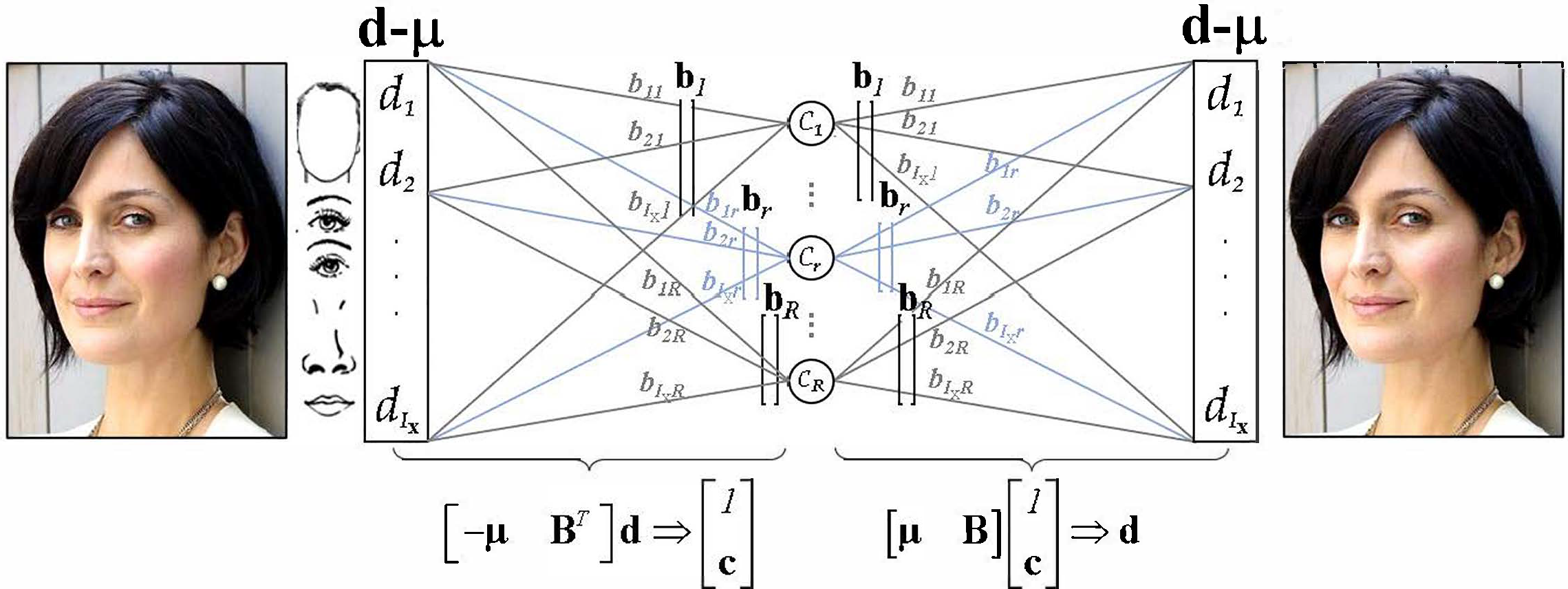
Figure 6: Autoencoder-decoder architecture and Principal Component Analysis. (All images have been vectorized, but they are displayed as a grid of numbers. )

The weights of a Hebb neuron, $c_{\mbox{\tiny{r}}}$, are updated by

$$\Delta{\mathbf{b}}_{\mbox{\tiny{r}}}(t+1)\hskip-7.22743pt = \hskip-7.22743pt\eta\left({\mathbf{d}}-{\sum_{i_{\mbox{\tiny{r}}}=1}^{r}}{\mathbf{b}}_{{i}_{\mbox{\tiny{r}}}}(t)c_{i_{\mbox{\tiny{r}}}}(t)\right)c_{\mbox{\tiny{r}}}(t)$$

$$= \hskip-7.22743pt\eta\left({\mathbf{d}}-{\sum_{i_{\mbox{\tiny{r}}}=1}^{r}}{\mathbf{b}}_{i_{\mbox{\tiny{r}}}}(t){\mathbf{b}}{}^{\hbox{\tiny{T}}}_{i_{\mbox{\tiny{r}}}}(t){\mathbf{d}}\right){\mathbf{d}}{}^{\hbox{\tiny{T}}}{\mathbf{b}}_{r}(t),$$

$${\mathbf{b}}_{\mbox{\tiny{r}}}(t+1) = \hskip-7.22743pt\frac{\left({\mathbf{b}}_{\mbox{\tiny{r}}}(t)+\Delta{\mathbf{b}}_{\mbox{\tiny{r}}}(t+1)\right)}{\|{\mathbf{b}}_{\mbox{\tiny{r}}}(t)+\Delta{\mathbf{b}}_{\mbox{\tiny{r}}}(t+1)\|}$$

where ${\mathbf{d}}\in\mathbb{C}^{I_{\mbox{\tiny{0}}}}$ is a vectorized centered observation with $I_{\mbox{\tiny{0}}}$ measurements, $0\leq\eta\leq{2}/{\|B\|^{2}}=\sigma_{\mbox{\tiny{max,B}}}$ is the learning rate, ${\mathbf{b}}_{\mbox{\tiny{r}}}$ are the autoencoder weights of the $r^{\hbox{\small th}}$ neuron, $c_{\mbox{\tiny{r}}}$ is the activation, and $t$ is the time iteration. Back-propagation[64, 65] performs PCA gradient descent [19, p. 58][51]. An autoencoder may be trained and the weights updated with a data batch, ${\mathbf{D}}$,

$$\Delta{\mathbf{b}}_{\mbox{\tiny{i}}}\mbox{\small$(t+1)$} = \left({\mathbf{D}}-{\mathbf{B}}_{\mbox{\tiny{r}}}\mbox{\small$(t)$}{\mathbf{B}}{}^{\hbox{\tiny{T}}}_{\mbox{\tiny{r}}}\mbox{\small$(t)$}{\mathbf{D}}\right){\mathbf{D}}{}^{\hbox{\tiny{T}}}{\mathbf{b}}_{\mbox{\tiny{r}}}\mbox{\small$(t)$}$$

$$= \left({\mathbf{D}}{\mathbf{D}}{}^{\hbox{\tiny{T}}}-{\sum_{i_{\mbox{\tiny{r}}}=1}^{r}}{\mathbf{b}}_{i_{\mbox{\tiny{r}}}}\mbox{\small$(t)$}{\mathbf{b}}{}^{\hbox{\tiny{T}}}_{i_{\mbox{\tiny{r}}}}\mbox{\small$(t)$}{\mathbf{D}}{\mathbf{D}}{}^{\hbox{\tiny{T}}}\right){\mathbf{b}}_{r}\mbox{\small$(t)$}.$$

Computational speed-ups are achieved with stochastic gradient descent [12][80].

VI-B Relevant Tensor Algebra

Briefly, the natural generalization of matrices (i.e., linear operators defined over a vector space), tensors define multilinear operators over a set of vector spaces. A “data tensor” denotes an $M$-way data array.

Definition 1 (Tensor)

Tensors are multilinear mappings over a set of vector spaces, $\mathbb{C}^{I_{\mbox{\tiny{m}}}}$, $1\leq m\leq M$, to a range vector space $\mathbb{C}^{I_{0}}$:

$$\hskip 36.135pt{\mathbf{\mathcal{A}}}:\left\{\mathbb{C}^{I_{1}}\times\mathbb{C}^{I_{2}}\times\dots\times\mathbb{C}^{I_{\mbox{\tiny{M}}}}\right\}\mapsto\mathbb{C}^{I_{0}}.$$ (32)

The order of tensor ${\mathbf{\mathcal{A}}}\in\mathbb{C}^{I_{0}\times I_{1}\times\dots\times I_{\mbox{\tiny{M}}}}$ is $M+1$. An element of ${\mathbf{\mathcal{A}}}$ is denoted as ${\mathbf{\mathcal{A}}}_{i_{0}i_{1}\dots i_{\mbox{\tiny{m}}}\dots i_{\mbox{\tiny{M}}}}$ or $a_{i_{0}i_{1}\dots i_{\mbox{\tiny{m}}}\dots i_{\mbox{\tiny{M}}}}$, where $1\leq i_{\mbox{\tiny{m}}}\leq I_{\mbox{\tiny{m}}}$.

The mode-$m$ vectors of an $M^{\hbox{\small th}}$-order tensor ${\mathbf{\mathcal{A}}}\in\mathbb{C}^{I_{0}\times I_{1}\times\dots\times I_{\mbox{\tiny{M}}}}$ are the $I_{\mbox{\tiny{m}}}$-dimensional vectors obtained from ${\mathbf{\mathcal{A}}}$ by varying index $i_{\mbox{\tiny{m}}}$ while keeping the other indices fixed. In tensor terminology, column vectors are the mode-0 vectors and row vectors as mode-1 vectors. The mode-$m$ vectors of a tensor are also known as fibers. The mode-$m$ vectors are the column vectors of matrix ${{\mathbf{A}}}_{\mbox{\tiny{$[m]$}}}$ that results from matrixizing (a.k.a. flattening) the tensor ${\mathbf{\mathcal{A}}}$.

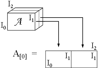
Figure 7: Matrixizing a $3^{\hbox{\small rd}}$ order tensor, ${\mathbf{\mathcal{A}}}$.

Definition 2 (Mode-$m$ Matrixizing)

The mode-$m$ matrixizing of tensor ${\mathbf{\mathcal{A}}}\in\mathbb{C}^{I_{0}\times I_{1}\times\dots I_{\mbox{\tiny{M}}}}$ is defined as the matrix ${{\mathbf{A}}}_{\mbox{\tiny{$[m]$}}}\in\mathbb{C}^{I_{\mbox{\tiny{m}}}\times(I_{0}\dots I_{m-1}I_{m+1}\dots I_{\mbox{\tiny{M}}})}$. As the parenthetical ordering indicates, the mode-$m$ column vectors are arranged by sweeping all the other mode indices through their ranges, with smaller mode indexes varying more rapidly than larger ones; thus,

$$\hskip-27.10124pt\left[{{\mathbf{A}}}_{\mbox{\tiny{$[m]$}}}\right]_{jk}\hskip-3.61371pt=a_{i_{1}\dots i_{\mbox{\tiny{m}}}\dots i_{\mbox{\tiny{M}}}},\quad\mbox{where}$$ (33)

$$\hskip-10.84006pt\quad j=i_{\mbox{\tiny{m}}}\quad\mbox{and}\quad k=1+\sum_{n=0\atop n\neq m}^{M}(i_{n}-1)\prod_{l=0\atop l\neq m}^{n-1}I_{l}.\vspace{-.2in}$$

Input the data tensor ${\mathbf{\mathcal{D}}}\in\mathbb{C}^{I_{0}\times\dots\times I_{\mbox{\tiny{M}}}}$.

1. For $m\mathrel{\mathop{:}}=0,\dots,M$,
   Let ${\mathbf{U}}_{\mbox{\tiny{m}}}$ be the left orthonormal matrix of $\left[{\mathbf{U}}_{\mbox{\tiny{m}}}{\mathbf{S}}_{\mbox{\tiny{m}}}{\mathbf{V}}{}^{\hbox{\tiny{T}}}_{\mbox{\tiny{m}}}\right]\mathrel{\mathop{:}}=\mbox{svd}({{\mathbf{D}}}_{\mbox{\tiny{$[m]$}}})$

2. Set ${\mathbf{\mathcal{Z}}}\mathrel{\mathop{:}}={\mathbf{\mathcal{D}}}\times_{0}{\mathbf{U}}_{0}{}^{\hbox{\tiny{T}}}\times_{1}{\mathbf{U}}_{1}{}^{\hbox{\tiny{T}}}\dots\times_{\mbox{\tiny{m}}}{\mathbf{U}}_{\mbox{\tiny{m}}}{}^{\hbox{\tiny{T}}}...\times_{\mbox{\tiny{M}}}{\mathbf{U}}_{\mbox{\tiny{M}}}{}^{\hbox{\tiny{T}}}$.

Output mode matrices ${\mathbf{U}}_{0},{\mathbf{U}}_{\mbox{\tiny{1}}},...,{\mathbf{U}}_{\mbox{\tiny{M}}}$, and the core tensor ${\mathbf{\mathcal{Z}}}$.

Algorithm 3 $M$-mode SVD algorithm.[105]

A generalization of the product of two matrices is the product of a tensor and a matrix [25, 18].

Definition 3 (Mode-$m$ Product, $\times_{\mbox{\tiny{m}}}$)

The mode-$m$ product of a tensor ${\mathbf{\mathcal{A}}}\in\mathbb{C}^{I_{1}\times I_{2}\times\dots\times I_{\mbox{\tiny{m}}}\times\dots\times I_{\mbox{\tiny{M}}}}$ and a matrix ${\mathbf{B}}\in\mathbb{C}^{J_{\mbox{\tiny{m}}}\times I_{\mbox{\tiny{m}}}}$, denoted by ${\mathbf{\mathcal{A}}}\times_{\mbox{\tiny{m}}}{\mathbf{B}}$, is a tensor of dimensionality $\mathbb{C}^{I_{1}\times\dots\times I_{m-1}\times J_{\mbox{\tiny{m}}}\times I_{m+1}\times\dots\times I_{\mbox{\tiny{M}}}}$ whose entries are computed by

$$\vspace{-.1in}[{\mathbf{\mathcal{A}}}\times_{\mbox{\tiny{m}}}{\mathbf{B}}]_{i_{1}...i_{m-1}j_{\mbox{\tiny{m}}}i_{m+1}...i_{\mbox{\tiny{M}}}} = \sum_{i_{\mbox{\tiny{m}}}}a_{i_{1}...i_{m-1}i_{\mbox{\tiny{m}}}i_{m+1}...i_{\mbox{\tiny{M}}}}b_{j_{\mbox{\tiny{m}}}i_{\mbox{\tiny{m}}}},$$

$$\vspace{-.2in}{\mathbf{\mathcal{C}}}={\mathbf{\mathcal{A}}}\times_{\mbox{\tiny{m}}}{\mathbf{B}}.\hskip 3.61371pt \mathrel{\vbox{\hbox{ \leavevmode\hbox to46.62pt{\vbox to26.24pt{\text{[drawing]}}} }}} {{\mathbf{C}}}_{\mbox{\tiny{$[m]$}}}={\mathbf{B}}{{\mathbf{A}}}_{\mbox{\tiny{$[m]$}}}.\vspace{-.25in}$$ (38)

The $M$-mode SVD, Algorithm 3 proposed by Vasilescu and Terzopoulos [105] is a “generalization” of the conventional matrix (i.e., 2-mode) SVD which may be written in tensor notation as

$$\vspace{+.035in}\hskip-18.06749pt{\mathbf{D}}={\mathbf{U}}_{0}{\mathbf{S}}{\mathbf{U}}_{1}{}^{\hbox{\tiny{T}}}\hskip 14.45377pt\Leftrightarrow\hskip 14.45377pt{\mathbf{D}}={\mathbf{S}}\times_{0}{\mathbf{U}}_{0}\times_{1}{\mathbf{U}}_{1}\vspace{+.035in}$$

The $M$-mode SVD orthogonalizes the $M$ spaces and decomposes a tensor as the mode-m product, denoted $\times_{\mbox{\tiny{m}}}$ , of $M$-orthonormal mode matrices, and a core tensor ${\mathbf{\mathcal{Z}}}$

$$\hskip-21.68121pt{\mathbf{\mathcal{D}}} \hskip-7.22743pt= \hskip-7.22743pt{{\mathbf{\mathcal{Z}}}}\times_{0}{{\mathbf{U}}}_{0}\dots\times_{\mbox{\tiny{m}}}{{\mathbf{U}}}_{\mbox{\tiny{m}}}\dots\times_{\mbox{\tiny{M}}}{{\mathbf{U}}}_{\mbox{\tiny{M}}}.$$ (39)

$${{\mathbf{D}}}_{\mbox{\tiny{$[m]$}}} \hskip-7.22743pt= \hskip-7.22743pt{\mathbf{U}}_{\mbox{\tiny{m}}}{{\mathbf{Z}}}_{\mbox{\tiny{$[m]$}}}\left({{\mathbf{U}}}_{\mbox{\tiny{M}}}\dots\otimes{{\mathbf{U}}}_{\mbox{\tiny{m+1}}}\otimes_{\mbox{\tiny{m-1}}}{{\mathbf{U}}}\dots\otimes{{\mathbf{U}}}_{0}\right){}^{\hbox{\tiny{T}}},$$ (40)

$$vec({\mathbf{\mathcal{D}}}) \hskip-7.22743pt= \hskip-7.22743pt\left({{\mathbf{U}}}_{\mbox{\tiny{M}}}\dots\otimes{{\mathbf{U}}}_{\mbox{\tiny{m+1}}}\otimes{{\mathbf{U}}}_{\mbox{\tiny{m-1}}}\dots\otimes{{\mathbf{U}}}_{0}\right)vec({\mathbf{\mathcal{Z}}}).$$ (41)

The latter two equations express the decomposition in matrix form and in terms of $vec$ operators.

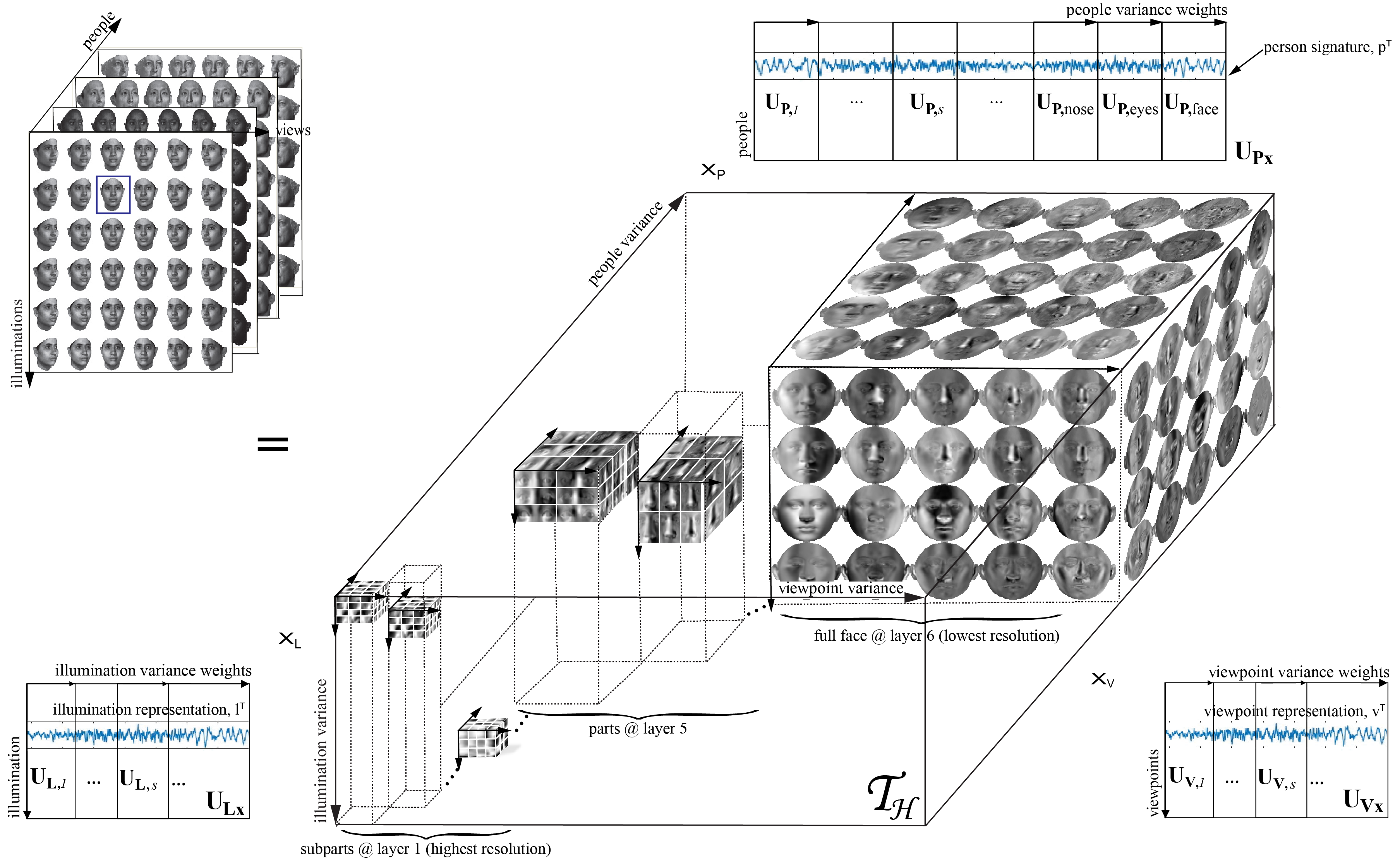
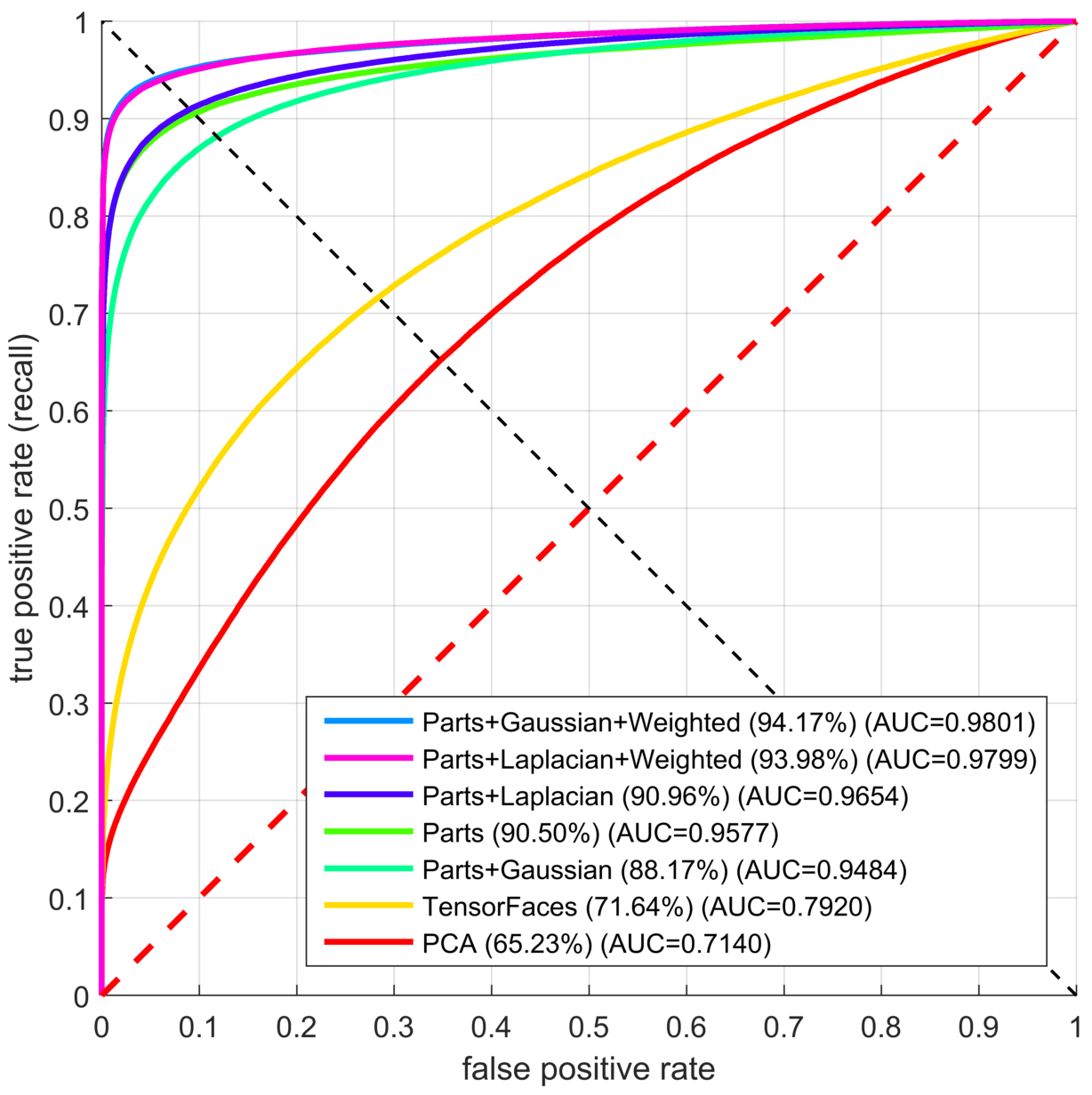
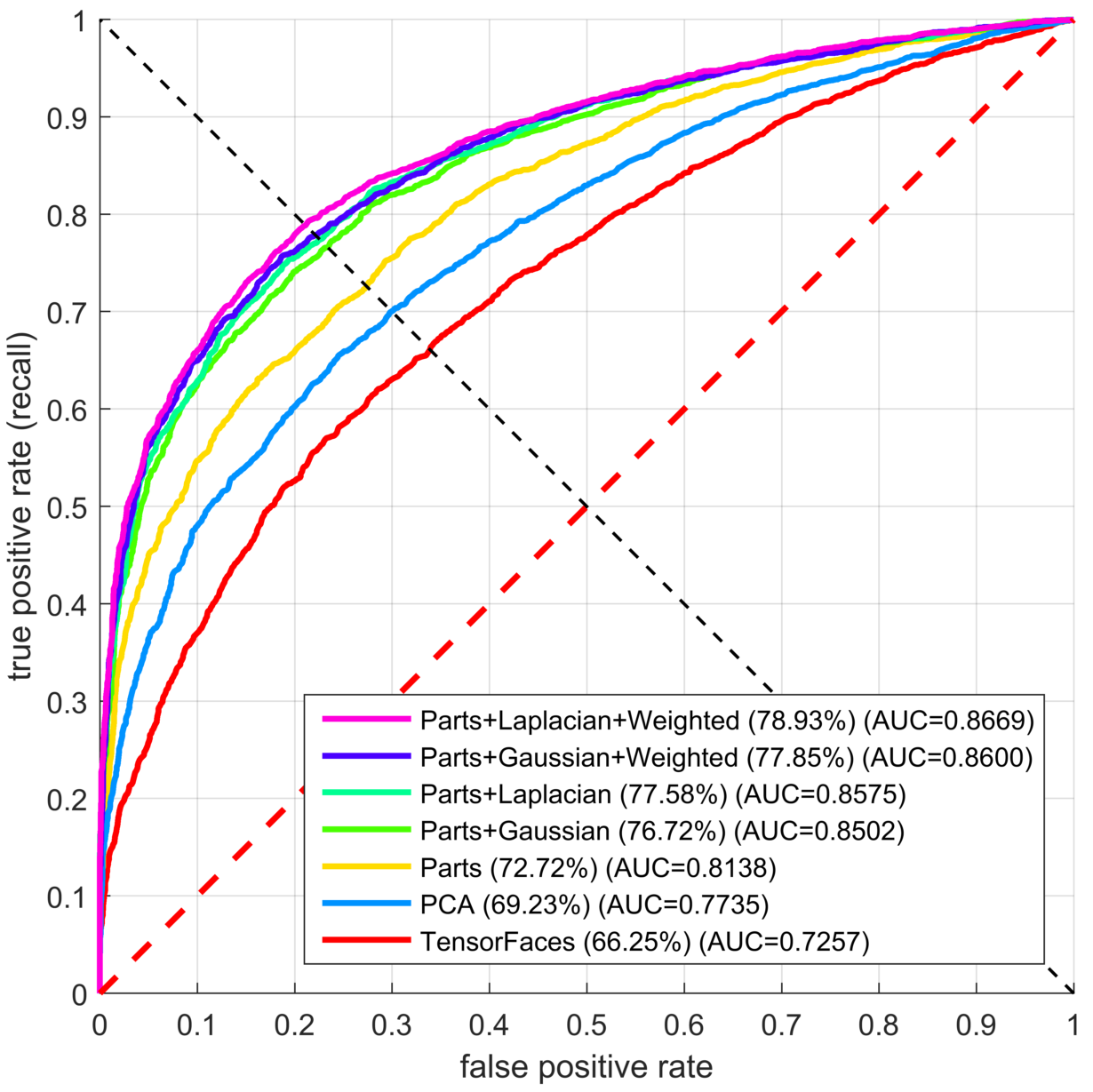
                (b)                   (c)

Figure 8: Compositional Hierarchical Block TensorFaces learns a hierarchy of features, and reesents each person as a part-based compositional representation. Figure depicts the training data factorization, ${\mathbf{\mathcal{D}}}={\mathbf{\mathcal{T}}}{{}_{\mbox{\tiny${\mathbf{\mathcal{H}}}$}}}\times_{\mbox{\tiny{L}}}{\mathbf{U}}_{\mbox{\tiny{L}}}\times_{\mbox{\tiny{V}}}{\mathbf{U}}_{\mbox{\tiny{V}}}\times_{\mbox{\tiny{P}}}{\mathbf{U}}_{\mbox{\tiny{P}}}$, where an observation is represented as ${\mathbf{d}}({\mathbf{p}},{\mathbf{v}},{\mathbf{l}})={\mathbf{\mathcal{T}}}{{}_{\mbox{\tiny${\mathbf{\mathcal{H}}}$}}}\times_{\mbox{\tiny{L}}}{\mathbf{l}}{}^{\hbox{\tiny{T}}}\times_{\mbox{\tiny{V}}}{\mathbf{v}}{}^{\hbox{\tiny{T}}}\times_{\mbox{\tiny{P}}}{\mathbf{p}}{}^{\hbox{\tiny{T}}}$ and ${\mathbf{\mathcal{T}}}_{\mbox{\tiny${\mathbf{\mathcal{H}}}$}}$ spans the hierarchical causal factor variance. (b) ROC curves for the University of Freiburg 3D Morphable Faces dataset. (c) ROC curves for the LFW dataset. The average accuracies are listed next to each method, along with the area under the curve (AUC). Parts refers to using compositional hierarchical Block TensorFaces models to separately analyze facial parts. Gaussian, Laplacian refers to using compositional hierarchical Block TensorFaces on a Gaussian/Laplacian data pyramid.

Training Dataset	Test Dataset	PCA	TensorFaces	Compositional Hierarchical Block TensorFaces
				Pixels	Gaussian Pyramid	Weighted Gaussian Pyramid	Laplacian Pyramid	Weighted Laplacian Pyramid
Freiburg	Freiburg	65.23%	71.64%	90.50%	88.17%	94.17%	90.96%	93.98%
Freiburg	LFW (grey level images)	69.23% $\scriptstyle\pm$1.51	66.25% $\scriptstyle\pm$1.60	72.72% $\scriptstyle\pm$2.14	76.72% $\scriptstyle\pm$1.65	77.85% $\scriptstyle\pm$1.83	77.58% $\scriptstyle\pm$1.45	78.93% $\scriptstyle\pm$1.77

Figure 9: Empirical results reported for Freiburg and Labeled Faces in the Wild (LFW) using PCA, TensorFaces and Compositional Hierarchical Block TensorFaces representations. Pixels denotes independent facial part analysis Gaussian/Laplacian use a multi resolution pyramid to analyze facial features at different scales. Weighted denotes a weighted composite signature.
Freiburg Experiment:
Train on Freiburg: 6 views ($\scriptstyle\pm$60^∘,$\scriptstyle\pm$30^∘,$\scriptstyle\pm$5^∘); 6 illuminations ($\scriptstyle\pm$60^∘,$\scriptstyle\pm$30^∘,$\scriptstyle\pm$5^∘), 45 people
Test on Freiburg:    9 views ($\scriptstyle\pm$50^∘, $\scriptstyle\pm$40^∘, $\scriptstyle\pm$20^∘, $\scriptstyle\pm$10^∘, 0^∘), 9 illums ($\scriptstyle\pm$50^∘, $\scriptstyle\pm$40^∘, $\scriptstyle\pm$20^∘, $\scriptstyle\pm$10^∘, 0^∘), 45 different people
Labeled Faces in the Wild (LFW) Experiment:
Models were trained on approximately half of one percent ($0.5\%<1\%$) of the $4.4$M images used to train DeepFace.
Train on Freiburg:
15 views ($\scriptstyle\pm$60^∘,$\scriptstyle\pm$50^∘, $\scriptstyle\pm$40^∘,$\scriptstyle\pm$30^∘, $\scriptstyle\pm$20^∘, $\scriptstyle\pm$10^∘,$\scriptstyle\pm$5^∘, 0^∘), 15 illuminations ($\scriptstyle\pm$60^∘,$\scriptstyle\pm$50^∘, $\scriptstyle\pm$40^∘,$\scriptstyle\pm$30^∘, $\scriptstyle\pm$20^∘, $\scriptstyle\pm$10^∘,$\scriptstyle\pm$5^∘, 0^∘), 100 people
Test on LFW: We report the mean accuracy and standard deviation across standard literature partitions [43], following the
Unrestricted, labeled outside data supervised protocol.

VI-C Compositional Hierarchical Block TensorFaces

Training Data: In our experiments, we employed gray-level facial training images rendered from 3D scans of 100 subjects. The scans were recorded using a CyberwareTM 3030PS laser scanner and are part of the 3D morphable faces database created at the University of Freiburg [11]. Each subject was combinatoriall y imaged in Maya from 15 different viewpoints ($\theta=-60^{\circ}$ to $+60^{\circ}$ in $10^{\circ}$ steps on the horizontal plane, $\phi=0^{\circ}$) with $15$ different illuminations ( $\theta=-35^{\circ}$ to $+35^{\circ}$ in $5^{\circ}$ increments on a plane inclined at $\phi=45^{\circ}$).

Data Preprocessing: Facial images were warped to an average face template by a piecewise affine transformation given a set of facial landmarks obtained by employing Dlib software [57, 53, 88, 67, 35]. Illumination was normalized with an adaptive contrast histogram equalization algorithm, but rather than performing contrast correction on the entire image, subtiles of the image were contrast normalized, and tiling artifacts were eliminated through interpolation. Histogram clipping was employed to avoid over-saturated regions.

Experiments:We ran five experiments with five facial part-based hierarchies from which a person representation was computed, Fig. 9. Each image, ${\mathbf{d}}\in\mathbb{R}^{I_{\mbox{\tiny{0}}}\times 1}$, was convolved with a Gaussian and a Laplacian filter bank $\{{\mathbf{H}}_{\mbox{\tiny{s}}}\|s=1...S\}$ that contained five filters, $S=5$. The filtered images, ${\mathbf{d}}\times_{\mbox{\tiny{0}}}{\mathbf{H}}_{\mbox{\tiny{s}}}$, resulted in five facial part hierarchies composed of (i) independent pixel parts (ii) parts segmented from different layers of a Gaussian pyramid that were equally or (iii) unequally weighed, (iv) parts were segmented from a Laplacian pyramid that were equally or (v) unequally weighed.

The composite person signature was computed for every test image by employing the multilinear projection algorithm [101, 109], and signatures were compared with a nearest neighbor classifier.

To validate the effectiveness of our system on real-world images, we report results on “LFW” dataset (LFW) [43]. This dataset contains 13,233 facial images of 5,749 people. The photos are unconstrained (i.e., “in the wild”), and include variation due to pose, illumination, expression, and occlusion. The dataset consists of 10 train/test splits of the data. We report the mean accuracy and standard deviation across all splits in Table 9. Fig. 9(b-c) depicts the experimental ROC curves. We follow the supervised “Unrestricted, labeled outside data” framework.

Results: While we cannot celebrate closing the gap on human performance, our results are promising. DeepFace, a CNN model, improved the prior art verification rates on LFW from $70\%$ to $97.35\%$, by training on $4.4M$ images of $200\times 200$ pixels from $4,030$ people, the same order of magnitude as the number of people in the LFW database.

We trained on less than one percent ($1\%$) of the $4.4$M total images used to train DeepFace. Images were rendered from 3D scans of 100 subjects with an the intraocular distance of approximately 20 pixels and with a facial region captured by $10,414$ pixels (image size $\approx 100\times 100$ pixels). We have currently achieved verification rates just shy of $80\%$ on LFW.

Summary: Compositional Hierarchical Block TensorFaces models cause-and-effect as a hierarchical block tensor interaction between intrinsic and extrinsic causal factors of data formation [103][98].

A data tensor expressed as a part-based a hierarchy is a unified tensor model of wholes and parts. The resulting causal factor representations are interpretable, hierarchical, and statistically invariant to all other causal factors. While we have not closed the gap on human performance, we report encouraging face verification results on two test data sets–the Freiburg, and the Labeled Faces in the Wild datasets by training on a very small set of synthetic images. We have currently achieved verification rates just shy of eighty percent on LFW by employing synthetic images from 100 people, 15 viewpoints and 15 illuminations, for a total that constitutes less than one percent ($1\%$) of the total images employed by DeepFace. CNN verification rates improved the $70\%$ prior art to $97.35\%$ only when they employed $4.4$M images from $4,030$ people, the same order of magnitude as the number of people in the LFW database.

References

- [1] D. H. Ackley, G. A. Hinton, and T. J. Sejnowski. A learning algorithm for Boltzmann machines. Cognitive Science, 9(1):147–169, 1985.
- [2] J. D. Angrist. Lifetime earnings and the vietnam era draft lottery: evidence from social security administrative records. The American Economic Review, pages 313–336, 1990.
- [3] F. R. Bach and M. I. Jordan. Kernel independent component analysis. Journal of Machine Learning Research, 3(Jul):1–48, 2002.
- [4] P. Baldi and K. Hornik. Neural networks and principal component analysis: Learning from examples without local minima. Neural networks, 2(1):53–58, 1989.
- [5] M. Bartlett, J. Movellan, and T. Sejnowski. Face recognition by independent component analysis. IEEE Transactions on Neural Networks, 13(6):1450–64, 2002.
- [6] A. J. Bell and T. J. Sejnowski. An information-maximization approach to blind separation and blind deconvolution. Neural Computation, (6):1004–1034, 1995.
- [7] J. Benesty, C. Paleologu, L. Dogariu, and S. Ciochină. Identification of linear and bilinear systems: A unified study. Electronics, 10(15), 2021.
- [8] Y. Bengio and A. Courville. Handbook on Neural Information Processing, chapter 1.Deep Learning of Representations, pages 1–28. Springer Berlin Heidelberg, Berlin, Heidelberg, 2013.
- [9] Y. Bengio, P. Lamblin, D. Popovici, H. Larochelle, and U. Montreal. Greedy layer-wise training of deep networks. volume 19, 01 2007.
- [10] P. Bentler and S. Lee. A statistical development of three-mode factor analysis. British J. of Math. and Stat. Psych., 32(1):87–104, 1979.
- [11] V. Blanz and T. A. Vetter. Morphable model for the synthesis of 3D faces. In Proc. ACM SIGGRAPH 99 Conf., pages 187–194, 1999.
- [12] L. Bottou et al. Online learning and stochastic approximations. On-line learning in neural networks, 17(9):142, 1998.
- [13] R. Bro. Parafac: Tutorial and applications. In Chemom. Intell. Lab Syst., Special Issue 2nd Internet Cont. in Chemometrics (INCINC’96), volume 38, pages 149–171, 1997.
- [14] A. Bulat, J. Kossaifi, G. Tzimiropoulos, and M. Pantic. Incremental multi-domain learning with network latent tensor factorization. In The Thirty-Fourth AAAI Conference on Artificial Intelligence, AAAI, pages 10470–10477. AAAI Press, 2020.
- [15] C. Cadieu and B. Olshausen. Learning transformational invariants from natural movies. In Proc. 19th Inter. Conf. on Neural Information Processing Systems, NIPS’09, page 209–216, 2009.
- [16] D. Card and A. B. Krueger. Minimum wages and employment: A case study of the fast food industry in New Jersey and Pennsylvania, 1993.
- [17] J. D. Carroll and J. J. Chang. Analysis of individual differences in multidimensional scaling via an N-way generalization of ‘Eckart-Young’ decomposition. Psychometrika, 35:283–319, 1970.
- [18] J. D. Carroll, S. Pruzansky, and J. B. Kruskal. CANDELINC: A general approach to multidimensional analysis of many-way arrays with linear constraints on parameters. Psychometrika, 45:3–24, 1980.
- [19] C. Chatfield and A. Collins. Introduction to Multivariate Analysis, 1983.
- [20] J. C. Chen, R. Ranjan, A. Kumar, C. H. Chen, V. M. Patel, and R. Chellappa. An end-to-end system for unconstrained face verification with deep convolutional neural networks. In IEEE International Conf. on Computer Vision Workshop (ICCVW), pages 360–368, Dec 2015.
- [21] W. Chu and Z. Ghahramani. Probabilistic models for incomplete multi-dimensional arrays. volume 5 of Proceedings of Machine Learning Research, pages 89–96, Hilton Clearwater Beach Resort, Clearwater Beach, Florida USA, 16–18 Apr 2009. PMLR.
- [22] D. C. Cireşan, U. Meier, J. Masci, L. M. Gambardella, and J. Schmidhuber. Flexible, high performance convolutional neural networks for image classification. In Proceedings of the Twenty-Second International Joint Conference on Artificial Intelligence - Volume Volume Two, IJCAI’11, page 1237–1242. AAAI Press, 2011.
- [23] P. Common. Independent component analysis, a new concept? Signal Processing, 36:287–314, 1994.
- [24] J. Davis and H. Gao. Recognizing human action efforts: An adaptive three-mode PCA framework. In Proc. IEEE Inter. Conf. on Computer Vision, (ICCV), pages 1463–69, Nice, France, Oct 13-16 2003.
- [25] L. de Lathauwer. Signal Processing Based on Multilinear Algebra. PhD dissertation, Katholieke Univ. Leuven, Belgium, 1997.
- [26] L. De Lathauwer, P. Comon, B. De Moor, and J. Vandewalle. Higher-order power method - application in independent component analysis. Proc. of the International Symposium on Nonlinear Theory and its Applications (NOLTA’95), pages 91–96, 1995.
- [27] A. P. Dempster, N. M. Laird, and D. B. Rubin. Maximum likelihood from incomplete data via the em algorithm. Journal of the Royal Statistical Society: Series B (Methodological), 39(1):1–22, 1977.
- [28] G. Desjardins, A. Courville, and Y. Bengio. Disentangling factors of variation via generative entangling. arXiv:1210.5474, 2012.
- [29] H. Fan, B. Xiong, K. Mangalam, Y. Li, Z. Yan, J. Malik, and C. Feichtenhofer. Multiscale vision transformers. In Proceedings of the IEEE/CVF International Conference on Computer Vision, pages 6824–6835, 2021.
- [30] R. P. Feynman. Knowing versus Understanding. 1961.
- [31] T. Gebru, J. Morgenstern, B. Vecchione, J. W. Vaughan, H. Wallach, H. D. III, and K. Crawford. Datasheets for datasets. Communications of the ACM, 64(12):86–92, 2021.
- [32] A. Gelman and G. Imbens. Why ask why? Forward causal inference and reverse causal questions. Tech.report, Nat.Bureau of Econ. Research, 2013.
- [33] G. Grindlay and M. A. O. Vasilescu. A multilinear (tensor) framework for hrtf analysis and synthesis. In 2007 IEEE International Conference on Acoustics, Speech and Signal Processing - ICASSP ’07, volume 1, pages I–161–164, 2007.
- [34] R. Harshman. Foundations of the PARAFAC procedure: Model and conditions for an explanatory factor analysis. Tech. Report Working Papers in Phonetics 16, UCLA, CA, Dec 1970.
- [35] A. Hatamizadeh, D. Terzopoulos, and A. Myronenko. End-to-end boundary aware networks for medical image segmentation. In Inter. Workshop on Machine Learning in Medical Imaging, pages 187–194. Springer, 2019.
- [36] D. O. Hebb. The organization of behavior: A neuropsychological theory. John Wiley And Sons, Inc., New York, 1949.
- [37] G. E. Hinton, S. Osindero, and Y.-W. Teh. A fast learning algorithm for deep belief nets. Neural Comput., 18(7):1527–54, Jul 2006.
- [38] G. E. Hinton and R. R. Salakhutdinov. Reducing the dimensionality of data with neural networks. Science, 313(5786):504–507, 2006.
- [39] P. W. Holland. Statistics and causal inference: Rejoinder. J. of the American Statistical Association, 81(396):968–970, 1986.
- [40] R. C. Hoover, K. Caudle, and K. Braman. A new approach to multilinear dynamical systems and control, 2021.
- [41] E. Hsu, K. Pulli, and J. Popovic. Style translation for human motion. ACM Transactions on Graphics, 24(3):1082–89, 2005.
- [42] G. B. Huang. Learning hierarchical representations for face verification with convolutional deep belief networks. In IEEE Conf. on Computer Vision and Pattern Recognition (CVPR), pages 2518–25, Jun 2012.
- [43] G. B. Huang, M. Ramesh, T. Berg, and E. Learned-Miller. Labeled faces in the wild: A database for studying face recognition in unconstrained environments. Technical Report 07-49, University of Massachusetts, Amherst, Oct 2007.
- [44] H.Wang and N.Ahuja. Facial expression decomposition. In Proc, 9th IEEE Inter. Conf. on Computer Vision (ICCV), pages 958–65,v.2, 2003.
- [45] A. Hyvärinen, J. Karhunen, and E. Oja. Independent Component Analysis. Wiley, New York, 2001.
- [46] G. Imbens and D. Rubin. Causal Inference for Statistics, Social and Biomedical Sciences: An Introduction. Cambridge Univ. Press, 2015.
- [47] G. W. Imbens and J. D. Angrist. Identification and estimation of local average treatment effects. Econometrica, 62(2):467–475, 1994.
- [48] L. Ingber. Simulated annealing: Practice versus theory. Mathematical and computer modelling, 18(11):29–57, 1993.
- [49] M. A. Iwen, D. Needell, E. Rebrova, and A. Zare. Lower memory oblivious (tensor) subspace embeddings with fewer random bits: modewise methods for least squares. SIAM Journal on Matrix Analysis and Applications, 42(1):376–416, 2021.
- [50] K. Jarrett, K. Kavukcuoglu, M. Ranzato, and Y. LeCun. What is the best multi-stage architecture for object recognition? In Proc. Inter. Conf. on Computer Vision (ICCV 2009), page 2146—53. IEEE, 2009.
- [51] I. Jolliffe. Principal Component Analysis. Springer-Verlag, New York, 1986.
- [52] A. Kapteyn, H. Neudecker, and T. Wansbeek. An approach to -mode component analysis. Psychometrika, 51(2):269–275, Jun 1986.
- [53] V. Kazemi and J. Sullivan. One millisecond face alignment with an ensemble of regression trees. In Proc. IEEE Conf. on Computer Vision and Pattern Recognition, CVPR ’14, pages 1867–74, Washington, DC, USA, 2014. IEEE Computer Society.
- [54] D. S. Kermany, M. Goldbaum, W. Cai, C. C. Valentim, H. Liang, S. L. Baxter, A. McKeown, G. Yang, X. Wu, F. Yan, J. Dong, M. K. Prasadha, J. Pei, M. Y. Ting, J. Zhu, C. Li, S. Hewett, J. Dong, I. Ziyar, A. Shi, R. Zhang, L. Zheng, R. Hou, W. Shi, X. Fu, Y. Duan, V. A. Huu, C. Wen, E. D. Zhang, C. L. Zhang, O. Li, X. Wang, M. A. Singer, X. Sun, J. Xu, A. Tafreshi, M. A. Lewis, H. Xia, and K. Zhang. Identifying medical diagnoses and treatable diseases by image-based deep learning. Cell, 172(5):1122–1131.e9, 2018.
- [55] V. Khrulkov. Geometrical Methods in Machine Learning and Tensor Analysis. PhD dissertation, Skolkovo Institute, 2020.
- [56] Y. Kim, E. Park, S. Yoo, T. Choi, L. Yang, and D. Shin. Compression of deep convolutional neural networks for fast and low power mobile applications. CoRR, abs/1511.06530, 2015.
- [57] D. E. King. Dlib-ml: A machine learning toolkit. Journal of Machine Learning Research, 10:1755–1758, 2009.
- [58] T. G. Kolda and B. W. Bader. Tensor decompositions and applications. SIAM review, 51(3):455–500, 2009.
- [59] J. Kossaifi, Z. C. Lipton, A. Kolbeinsson, A. Khanna, T. Furlanello, and A. Anandkumar. Tensor regression networks. Journal of Machine Learning Research, 21(123):1–21, 2020.
- [60] P. M. Kroonenberg and J. de Leeuw. Principal component analysis of three-mode data by means of alternating least squares algorithms. Psychometrika, 45:69–97, 1980.
- [61] H. Larochelle, D. Erhan, A. Courville, J. Bergstra, and Y. Bengio. An empirical evaluation of deep architectures on problems with many factors of variation. In Proceedings of the 24th International Conference on Machine Learning, page 473–480, New York, NY, USA, 2007.
- [62] V. Lebedev, Y. Ganin, M. Rakhuba, I. V. Oseledets, and V. S. Lempitsky. Speeding-up convolutional neural networks using fine-tuned cp-decomposition. CoRR, abs/1412.6553, 2014.
- [63] Y. LeCun, Y. Bengio, and G. Hinton. Deep learning. Nature, 521(7553):436–444, 2015.
- [64] Y. LeCun, L. Bottou, Y. Bengio, and P. Haffner. Gradient-based learning applied to document recognition. Proceedings of the IEEE, 86(11):2278–2324, Nov 1998.
- [65] Y. A. LeCun, L. Bottou, G. B. Orr, and K.-R. Müller. Efficient BackProp, pages 9–48. Springer Berlin Heidelberg, Berlin, Heidelberg, 2012.
- [66] Z. Liu, Y. Lin, Y. Cao, H. Hu, Y. Wei, Z. Zhang, S. Lin, and B. Guo. Swin transformer: Hierarchical vision transformer using shifted windows. In Proceedings of the IEEE/CVF International Conference on Computer Vision, pages 10012–10022, 2021.
- [67] I. Macedo, E. V. Brazil, and L. Velho. Expression transfer between photographs through multilinear aam’s. pages 239–246, Oct 2006.
- [68] A. Madani, M. Moradi, A. Karargyris, and T. Syeda-Mahmood. Semi-supervised learning with generative adversarial networks for chest x-ray classification with ability of data domain adaptation. In 2018 IEEE 15th International Symposium on Biomedical Imaging (ISBI 2018), pages 1038–1042, 2018.
- [69] J. Magnus and H. Neudecker. Matrix Differential Calculus with Applications in Statistics and Econometrics. John Wiley & Sons, 1988.
- [70] J. Masci, U. Meier, D. Cireşan, and J. Schmidhuber. Stacked convolutional auto-encoders for hierarchical feature extraction. In T. Honkela, W. Duch, M. Girolami, and S. Kaski, editors, Artificial Neural Networks and Machine Learning – ICANN 2011, pages 52–59, Berlin, Heidelberg, 2011. Springer Berlin Heidelberg.
- [71] M. F. Mathieu, J. J. Zhao, J. Zhao, A. Ramesh, P. Sprechmann, and Y. LeCun. Disentangling factors of variation in deep representation using adversarial training. Advances in neural information processing systems, 29, 2016.
- [72] R. Memisevic and G. E. Hinton. Learning to Represent Spatial Transformations with Factored Higher-Order Boltzmann Machines. Neural Computation, 22(6):1473–1492, 06 2010.
- [73] V. Nair and G. E. Hinton. 3D object recognition with deep belief nets. In Proc. 22Nd Inter. Conf. on Neural Information Processing Systems, NIPS’09, pages 1339–47, USA, 2009. Curran Associates Inc.
- [74] A. Novikov, D. Podoprikhin, A. Osokin, and D. P. Vetrov. Tensorizing neural networks. In C. Cortes, N. D. Lawrence, D. D. Lee, M. Sugiyama, and R. Garnett, editors, Advances in Neural Information Processing Systems 28, pages 442–450. Curran Associates, Inc., 2015.
- [75] E. Oja. A simplified neuron model as a principal component analyzer. 15:267–2735, 1982.
- [76] C. C. Onu, J. E. Miller, and D. Precup. A fully tensorized recurrent neural network. CoRR, abs/2010.04196, 2020.
- [77] I. V. Oseledets. Tensor-train decomposition. SIAM J. on Scientific Computing, 33(5):2295–2317, 2011.
- [78] J. Pearl. Causality: Models, Reasoning, and Inference. Cambridge Univ. Press, 2000.
- [79] M. Ranzato, C. Poultney, S. Chopra, and Y. LeCun. Efficient learning of sparse representations with an energy-based model. In Proc. 19th Inter. Conf. on Neural Information Processing Systems, NIPS’06, pages 1137–44, Cambridge, MA, USA, 2006. MIT Press.
- [80] H. Robbins and S. Monro. A stochastic approximation method. The annals of mathematical statistics, pages 400–407, 1951.
- [81] D. B. Rubin. For objective causal inference, design trumps experimental analysis. The Annals of Applied Statistics, 2(3):808 – 840, 2008.
- [82] D. E. Rumelhart, G. E. Hinton, and R. J. Williams. Learning internal representations by error propagation. 1986.
- [83] T. Sanger. Optimal unsupervised learnig in a single layer linear feedforward neural network. 12:459–473, 1989.
- [84] J. Schmidhuber. Deep learning in neural networks: An overview. Neural networks, 61:85–117, 2015.
- [85] B. Scholkopf, A. J. Smola, and K. R. Muller. Kernel principal component analysis. Lecture notes in computer science, 1327:583–588, 1997.
- [86] B. Schölkoph, A. Smola, and K.-R. Muller. Nonlinear component analysis as a kernel eigenvalue problem. Neural Computation, 10(5):1299–1319, 1998.
- [87] T. Sejnowski, S. Chattarji, and P. Sfanton. Induction of Synaptic Plasticity by Hebbian Covariance in the Hippocampus, pages 105–124. Addison-Wesley, 1989.
- [88] W. Si, K. Yamaguchi, and M. A. O. Vasilescu. Face Tracking with Multilinear (Tensor) Active Appearance Models. Jun 2013.
- [89] P. Spirtes, C. N. Glymour, R. Scheines, and D. Heckerman. Causation, prediction, and search. MIT press, 2000.
- [90] Y. Sun, X. Wang, and X. Tang. Hybrid deep learning for face verification. In Proc. IEEE International Conf. on Computer Vision (ICCV), pages 1489–96, Dec 2013.
- [91] Y. Taigman, M. Yang, M. Ranzato, and L. Wolf. Deepface: Closing the gap to human-level performance in face verification. In Proc. IEEE Conf. on Computer Vision and Pattern Recognition, pages 1701–08, 2014.
- [92] Y. Tang, R. Salakhutdinov, and G. Hinton. Tensor analyzers. volume 28 of Proceedings of Machine Learning Research, pages 163–171, Atlanta, Georgia, USA, 17–19 Jun 2013.
- [93] N. Tishby and N. Zaslavsky. Deep learning and the information bottleneck principle. In 2015 IEEE Information Theory Workshop (ITW), pages 1–5, 2015.
- [94] E. J. Topol. High-performance medicine: the convergence of human and artificial intelligence. Nature Medicine, 25(1):44–56, 2019.
- [95] L. R. Tucker. Some mathematical notes on three-mode factor analysis. Psychometrika, 31:279–311, 1966.
- [96] M. Vasilescu and D. Terzopoulos. Adaptive meshes and shells: Irregular triangulation, discontinuities, and hierarchical subdivision. In Proc. IEEE Conf. on Computer Vision and Pattern Recognition (CVPR’92), pages 829–832, Champaign, IL, Jun 1992.
- [97] M. A. O. Vasilescu. Human motion signatures: Analysis, Synthesis, Recognition. In Proc. Int. Conf. on Pattern Recognition, volume 3, pages 456–460, Quebec City, Aug 2002.
- [98] M. A. O. Vasilescu. Incremental Multilinear SVD. In Proc. Conf. on ThRee-way methods In Chemistry And Psychology (TRICAP 06), 2006.
- [99] M. A. O. Vasilescu. A Multilinear (Tensor) Algebraic Framework for Computer Graphics, Computer Vision, and Machine Learning. PhD dissertation, University of Toronto, 2009.
- [100] M. A. O. Vasilescu. Multilinear projection for face recognition via canonical decomposition. In Proc. IEEE Inter. Conf. on Automatic Face Gesture Recognition (FG 2011), pages 476–483, Mar 2011.
- [101] M. A. O. Vasilescu. Multilinear projection for face recognition via canonical decomposition. In Proc. IEEE Inter. Conf. on Automatic Face Gesture Recognition (FG 2011), pages 476–483, Mar 2011.
- [102] M. A. O. Vasilescu and E. Kim. Compositional hierarchical tensor factorization: Representing hierarchical intrinsic and extrinsic causal factors. In The 25th ACM SIGKDD Conf. on Knowledge Discovery and Data Mining (KDD 2019): Tensor Methods for Emerging Data Science Challenges Workshop, Aug. 5 2019.
- [103] M. A. O. Vasilescu, E. Kim, and X. S. Zeng. CausalX: Causal eXplanations and block multilinear factor analysis. In 2020 25th International Conference of Pattern Recognition (ICPR 2020), pages 10736–10743, Jan 2021.
- [104] M. A. O. Vasilescu and D. Terzopoulos. Multilinear analysis for facial image recognition. In Proc. Int. Conf. on Pattern Recognition, volume 2, pages 511–514, Quebec City, Aug 2002.
- [105] M. A. O. Vasilescu and D. Terzopoulos. Multilinear analysis of image ensembles: TensorFaces. In Proc. European Conf. on Computer Vision (ECCV 2002), pages 447–460, Copenhagen, Denmark, May 2002.
- [106] M. A. O. Vasilescu and D. Terzopoulos. Multilinear subspace analysis of image ensembles. In Proc. IEEE Conf. on Computer Vision and Pattern Recognition, volume II, pages 93–99, Madison, WI, 2003.
- [107] M. A. O. Vasilescu and D. Terzopoulos. TensorTextures: Multilinear Image-Based Rendering. ACM Transactions on Graphics, 23(3):336–342, Aug 2004. Proc. ACM SIGGRAPH 2004 Conf., Los Angeles, CA.
- [108] M. A. O. Vasilescu and D. Terzopoulos. Multilinear independent components analysis. In Proc. IEEE Conf. on Computer Vision and Pattern Recognition, pages 547–553, v.I, San Diego, CA, 2005.
- [109] M. A. O. Vasilescu and D. Terzopoulos. Multilinear projection for appearance-based recognition in the tensor framework. In Proc. 11th IEEE Inter. Conf. on Computer Vision (ICCV’07), pages 1–8, 2007.
- [110] J.-P. Vert, K. Tsuda, and B. Schölkopf. A primer on kernel methods. Kernel methods in computational biology, 47:35–70, 2004.
- [111] D. Vlasic, M. Brand, H. Pfister, and J. Popovic. Face transfer with multilinear models. ACM Transactions on Graphics (TOG), 24(3):426–433, Jul 2005.
- [112] H. Wang and N. Ahuja. A tensor approximation approach to dimensionality reduction. Inter. J. of Computer Vision, 6(3):217–29, Mar 2008.
- [113] W. Wang, E. Xie, X. Li, D.-P. Fan, K. Song, D. Liang, T. Lu, P. Luo, and L. Shao. Pyramid vision transformer: A versatile backbone for dense prediction without convolutions. In Proceedings of the IEEE/CVF International Conference on Computer Vision, pages 568–578, 2021.
- [114] J. Yang, X. Gao, D. Zhang, and J. Yang. Kernel ICA: An alternative formulation and its application to face recognition. Pattern Recognition, 38(10):1784–87, 2005.
- [115] J. Ye. Generalized low rank approximations of matrices. Machine Learning, 61(1):167–191, 2005.
- [116] Q. Zhao, G. Zhou, S. Xie, L. Zhang, and A. Cichocki. Tensor ring decomposition. arXiv preprint arXiv:1606.05535, 2016.