Guided Hybrid Quantization for Object Detection in Multimodal Remote Sensing Imagery via One-to-one Self-teaching

Abstract

Recently, deep convolution neural networks (CNNs) have promoted accuracy in the computer vision field. However, the high computation and memory cost prevents its development in edge devices with limited resources, such as intelligent satellites and unmanned aerial vehicles. Considering the computation complexity, we propose a Guided Hybrid Quantization with One-to-one Self-Teaching (GHOST) framework. More concretely, we first design a structure called guided quantization self-distillation (GQSD), which is an innovative idea for realizing lightweight through the synergy of quantization and distillation. The training process of the quantization model is guided by its full-precision model, which is time-saving and cost-saving without preparing a huge pre-trained model in advance. Second, we put forward a hybrid quantization (HQ) module to obtain the optimal bit width automatically under a constrained condition where a threshold for distribution distance between the center and samples is applied in the weight value search space. Third, in order to improve information transformation, we propose a one-to-one self-teaching (OST) module to give the student network a ability of self-judgment. A switch control machine (SCM) builds a bridge between the student network and teacher network in the same location to help the teacher to reduce wrong guidance and impart vital knowledge to the student. This distillation method allows a model to learn from itself and gain substantial improvement without any additional supervision. Extensive experiments on a multimodal dataset (VEDAI) and single-modality datasets (DOTA, NWPU, and DIOR) show that object detection based on GHOST outperforms the existing detectors. The tiny parameters ($<$9.7 MB) and Bit-Operations (BOPs) ($<$2158 G) compared with any remote sensing-based, lightweight or distillation-based algorithms demonstrate the superiority in the lightweight design domain. Our code and model will be released at https://github.com/icey-zhang/GHOST.

I Introduction

Object detection in aerial images plays an important role in military security aiming to locate interested objects (e.g., vehicles, airplanes) on the ground and identifying their categories [1]. From universal detectors for natural images such as YOLOv3 [2], Faster R-CNN [3], FCOS [4] are widely introduced in the field of remote sensing (RS); more and more dedicated detectors for RS scene are designed and improved with the requirements of objects tasks. However, the large complexity of the object detection network is under-investigated, which limits the practical deployment under resource-limited scenarios and bring a heavy burden to process massive multimodal images collected from satellites, drone, and airplanes. Hence, a series of compression schemes have been proposed to settle this problem, such as pruning [5], quantization [6, 7, 8] and distillation [9, 10].

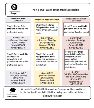
Figure 1: Comparison of training complexity, and accuracy between traditional distillation, traditional quantization and proposed mixed-bit self distillation (reported on VEDAI).

Quantization algorithms [11, 12] directly compress the cumbersome network, effectively reducing the computation cost and model size with a great compression potential. However, trivially applying quantization to CNNs usually leads to inferior performance if the compression bit decreases to a low level. Some knowledge distillation methods [13, 14, 15] are proven to be valid to elevate the performance of the lightweight model but have to pre-train a huge teacher model as a guidance of the student model which is time-consuming and resource-consuming [16]. Self-distillation methods [17, 16, 18] overcome this problem via the transfer of information inside the model itself without introducing extra huge storage and time consuming from the teacher model.

The above view naturally leads to a question: What research results will we get if we combine quantization and distillation by using a small full-precise network to guide the learning process of a quantization for this full-precision network? In this way, the tremendous compression capacity of quantified networks and the performance of full precision networks can be collaborative and cooperative.

In this paper, we design an adaptive one-to-one educational policy pertaining the full-precision network and the quantization network. We propose a simple yet novel approach that allows quantization network to reinforce presentation learning of itself relative full-precision network without the need of additional labels and external supervision. Our approach is named as Guided Hybrid Quantization with One-to-one Self-Teaching (GHOST) based on the guided quantization self-distillation (GQSD) framework. As the name implies, GHOST allows a network to exploit useful and vital knowledge derived from its own full-precision layers as the distillation targets for its quantization layers. GHOST opens a new possibility of training accurate tiny object detection networks.

As shown in Fig. 1, in order to train a small compact model to achieve as high accuracy as possible with less computation cost, we propose mixed-bit self distillation framework. Instead of implementing two steps in traditional distillation, which means that to train a large teacher model comes first, following by distilling the knowledge from it to the student model, we propose a two-step mixed-bit self distillation framework, in which the training process of the second quantization step is based on the pretrained small full-precision model. The proposed framework not only requires less computation cost (from 20797 G BOPs to 692 G BOPs on VEDAI dataset, a 30X faster training cost), but also can accomplish much higher accuracy (from 75.84% in traditional quantization to 80.31% on SuperYOLO) The main contributions of our work are as follows:

• We propose a unified guided quantization thought based on self-distillation called GQSD, which can tackle the lightweight object detectors’ quantization optimization problem in remote sensing. We are the first to formulate an adaptive one-to-one education policy between the full-precision network and the quantization network at the same structure in object detection.

• For the finding of weight value distribution features of remote sensing images, we design a hybrid quantization module, whose adaptive selection of the core information of the weights for quantization with a constrained preset condition can keep the balance of accuracy and efficiency.

• Aiming to offset the loss of the quantization information, the switch control machine is adopted to enable the student to distinguish and close the teacher’s wrong guidance and mine the correct and vital knowledge from self-distillation.

The rest of this paper is organized as follows: Section II give a rough overview of the spacific related work to this paper. Section III presents our proposed method in detail. Section IV introduces experimental results and analysis. Section V concludes this paper and discusses the future work.

II Related Work

In this section, we reviewed related work from object detection and network compression and acceleration in detail.

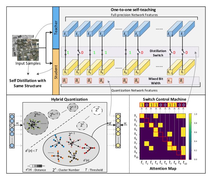
Figure 2: Overview of our proposed framework. An attention-based model determines similarities between the teacher and student features. Knowledge from each teacher feature is transferred to the student with similarities identified by Switch control machine (SCM) by self-distillation with the same structure. The mixed bit widths of the student network for quantization are based on the search results of the full-precision weights research space of teacher network in the same layer.

II-A Object Detection with Deep Learning

Various CNN-based object detection architectures have shown promising performance, bringing the field to a new level. The architectures can be roughly divided into two main domains: two-stage, and one-stage according to the change process of proposals.

Two-stage Detectors: A typical method is selective search work [19], where the first stage is to generate a large set of proposed region candidates that are required to cover the whole objects and then filter out most negative positions, and then the second stage is to complete classification for each region. R-CNN [20] creates a new era as one of the most successive two-stage algorithms owing to the upgrading of the second-stage classifier to a convolution network. Fast-RCNN [21] extractes features over the images before proposing regions and integrates the extractor and classifier by employing a soft layer rather than SVM classifier. Faster R-CNN [3] introduces a CNN-based region proposal network to further integrate proposal generation with the second-stage classifier into a single convolution network.

One-stage Detectors: One-stage detectors aim to jointly predict the classification and location of objects by integrating the detection and classification process. Recently, a series of SSD [22, 23, 24] and YOLO [25, 26, 2, 27] have renewed interest in the one-stage object detection. SSD implements independent detection on multiscale feature maps, while the YOLO utilizes combined detection. These methods have paid more attention to speed, but their accuracy trails behind that of tow-stage methods. YOLOv2 [26] modifies the location regression pattern depending on bounding boxes. YOLOv3 [2] considers multiscale objects and detects them in the three scales, which can realize the detection of multiple sizes of objects. YOLOv4 [27] introduces more data augmentation tricks, activation functions, backbone structures, and IoU loss metrics to enhance the robustness of the network. YOLOv5 [28] releases four different size models, where the basic structures are identical, which allows YOLOv5 to have higher flexibility and versatility in practical applications. To solve the dilemma of the category imbalance, RetinaNet [29] reduces the weight of massive amounts of simple negative samples in training by designing a focal term for cross-entropy loss. As FCOS [4] which belongs to anchor-free methods is proposed, adjusting hyperparameters and calculations related to anchor boxes has been avoided. ATSS [30] selects positive samples adaptively to enhance the detection performance.

II-B Deep Network Compression and Acceleration

Although the speed of the one-stage detection network is superior, its large model and high computation complexity still deserves to explore. Some researches focus on the design of a lightweight backbone. MobileNetV2 [31] utilizes the depthwise separable convolutions to build a lightweight model. ShuffleNet [32], and SqueezeNet [33] also effectively reduces the memory footprint during inference and speed up the detection. In the literature, a potential direction of model compression is knowledge distillation (KD) which concentrates on transferring knowledge from a heavy model (teacher) to a light one (teacher) to improve the light model’s performance without introducing extra costs [34, 35]. Whereas the knowledge distillation enables utilizing the larger network in a condensed manner, the pretraining of the large network requires extra substantial computation resources to prepare the teacher network [17]. The preparation of the pretrained teacher network is time-consuming and cost-consuming. The self-knowledge distillation [17, 16, 18] can overcome this problem by distilling its own knowledge without prior preparation of the teacher network. Quantization is another way to compact the model directly and compress the ponderous network by using low-bit representation. Mixed-precision quantization method uses different numbers of bits for a given data type to represent values in weight tensor. Many works [11, 36, 37, 37] have shown that the mixed-precision method is efficient for quantizing network layers that have different importance and sensitiveness for the bit width. However, trivially applying quantization to CNNs usually leads to inferior performance if the compression bit decreases to a low level.

III Network Architecture

In this section, we first revisit conventional KD and describe the proposed GHOST framework in Sec. III-A. Then, we present the details of the inspired hybrid quantization algorithm (Sec. III-B) and this quantization training process is guided by a one-to-one self-teaching method illustrated in Sec. III-C.

III-A Overview

KD is a widely-applied method that can be expressed as a knowledge transformer from teacher to student. Given a teacher model $\rm T$ and a student model $\rm S$, the $x$ is the data examples of models, here they can be the same for the teacher and the student model. In general, the KD machine can be uniformly expressed as:

$$\min{{\mathcal{L}}_{KD}}=\min\sum\limits_{{x_{i}}\in x}{\mathcal{L}}\left({{\rm{T}}\left({{x_{i}}}\right),{\rm{S}}\left({{x_{i}}}\right)}\right),$$ (1)

where $\mathcal{L}$ is the loss function that penalizes the differences between the teacher and the student.

The student model size is commonly designed in a small size to achieve the purpose of model compression in which the performance of the student can chase the teacher but consumes a computing-friendly resource. Nonetheless, the computation cost of the student model is larger than the pruning method directly completed on the teacher model. This demonstrates that the existing KD-based quantization algorithms still have great potential room for improvement.

We aim at developing a novel and generic baseline network with a focus on the learnable knowledge characteristics, making it well-applicable to the highly accurate and fine object detection of RS images with less computational costs. The key to model quantization with knowledge learning is to reduce the discrepancy which can be punished by distance or angle loss function between full-precision model $\rm P$ (teacher) and low-precision model $\rm Q$ (student) through optimizing $\rm Q$, which can be expressed as:

$$\mathrm{Q^{*}}=\min_{\mathrm{Q}}\sum_{x_{i}\in x}\mathcal{L}({\mathrm{P}}(x_{i}),{\mathrm{Q}}(x_{i})).$$ (2)

The weights of the teacher are frozen without gradient propagation when the teacher network guides the training of the student network. Based on the above presentation, we design an effective teacher-student distillation framework called GQSD which can be represented as:

$$\begin{split}\min\mathcal{L}_{KD}&=\min\sum\limits_{{x_{i}}\in x}\mathcal{L}({\rm P}({x_{i}}),{\rm Q}({x_{i}}),{\rm R}({x_{i}})),\\ s.t.&\quad W_{Q}=W_{init},B_{Q}=B.\end{split}$$ (3)

Specifically, the full precision network is the import fundamental teacher which not only provides the initial weights $W_{init}$ and bit width $B$ of the quantization model but also guides the quantization process to mine the vital knowledge from the teacher in specific features selected by a control ${\mathrm{R}}$. As shown in Fig 2, we propose a GHOST framework that concludes a hybrid quantization (HQ) module and a one-to-one self-teaching (OST) module. The mixed bit widths of the student network for quantization are based on the search results of the full-precision weights research space of the teacher network in the same layer. Inspired by the idea of harnessing intermediate features to improve performance in knowledge distillation [38, 39, 40], we design a Switch Control Machine (SCM) as ${\mathrm{R}}$ to generate an attention map that gains intermediate feature similarities between the teacher and student. The SCM controls the distillation switch and determines which knowledge should be delivered dynamically. Knowledge from each teacher feature is transferred to the student with similarities identified by SCM by self-distillation with the same structure. With a pretrained full-precision model as a initial weight, the quantization and distillation processes are conducted simultaneously to ultimately obtain a small lightweight model with little loss of accuracy. The details of the modules will be described separately as follows.

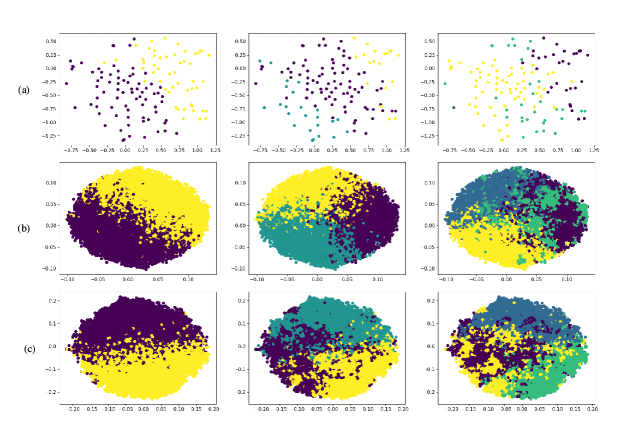
Figure 3: In the bottom layer of a trained network, the feature distributions of different categories intervene with each other severely as (a) shows. Many delicate neurons are needed to distinguish the overlapped distributions. And as the network propagates forward, the feature distribution of the same category gathers gradually in (b) and (c). At the end of the hidden layers, there exist clear margins between the semantic feature distributions of different classes in (d). With the improvement of separability among the feature manifolds, a neuron with lower-precision parameters is able to extract robust features.

III-B Hybrid Quantization

Powerful deep networks normally benefit from large model capacities but induce high computational and storage costs. Modal quantization is a promising approach to compress deep neural networks, making it possible to be deployed on edge devices. The quantization operator divides the weight into different fixed values by a quantization function which can be regarded as a cluster of convolution kernels in substance. The different scale weights are clustered to a certain value.

To illustrate this intuition explicitly, a SuperYOLO [41] network model which consists of 60 convolutional layers is trained based on the VEDAI dataset. After training, test samples are fed into the model. The convolution weight is firstly clustered into different categories by k-means and then transformed into 2 dimensions by t-SNE [42] to realize the visualization. As shown in Fig. 3, the convolution kernel weight in the (a) $0^{th}$, (b) $26^{th}$ and (c) $52^{nd}$ convolutional layer are clustered in different numbers. In Fig. 3 (a), the distance between different categories is relatively far which indicates that the weight distribution is dispersed and complicated in the initial layer. This is due to the fact that the color and texture features, which are detailed and multifarious, are captured in the shallow layer. As the layer propagates forward (Fig. 3 (b) and Fig. 3 (c)), the convolution weight becomes converging gradually. In other words, the semantic features in the deep layer are more robust and condensed so that with the deepening of the network layers, the clustering categories of weights can be relatively reduced.

Based on this finding, the hybrid quantization idea is introduced to search for the optimal bit width definition in the weight value space. We initially design a hyperparameter $T$ as a threshold to constrain the research space to control the compression rate of the quantization model. The search strategy can be described as:

$$\begin{split}B=&argmax(d(n))\\ s.t.&\quad d(n)<T.\end{split}$$ (4)

where the function $d(x)$ denotes the measurement of clustering extent at the $n$ bit width for each convolution layer. This definition aims to find the limited minimum clustering categories (maximum clustering extent) for each layer, hence the smallest quantization model with a minimum bit width is obtained at the preset ratio constraint. The hybrid quantization of the whole network definitely can be collected as:

$$B=[B^{1},B^{2},...,B^{l}]$$ (5)

where the $l$ is the total convolution layer and the $B_{l}$ is the $l^{t}h$ bit width of each layer weight parameter, and the bit width decreases progressively as the network propagates forward. We utilize the distribution distance defined as follows to determine the final bit width for quantization of the $l^{th}$ convolution layer weight:

$$d^{l}(n)=\frac{1}{M}\sum\limits_{j=0}^{M}{\sum\limits_{i=0}^{2^{n}}{{{({w^{l}_{ij}}-{c^{l}_{i}})}^{2}}}},$$ (6)

where the $M$ is the total number of kernel weights which correspond to $M=C_{in}\times C_{out}\times K\times K$. The $C_{in}$, $C_{out}$, and $K$ are the input channels, output channels and kernel size of the convolution layer. The whole weight values of each convolution layer complete the kmeans++ algorithm on the different cluster numbers. While the $2^{n}$ represents the cluster number. $c^{l}_{i}$ and $w^{l}_{ij}$ are the cluster centers and samples, as shown respectively in Fig. 4. We set the initial bit width as 8 and then select the superior and adaptive bit width by

$$B^{l}=\min(n|{d^{l}(n)}<T)\quad n=b_{min},b_{min}+1,...,8,$$ (7)

where the $b_{min}$ is a limit of the minimum bit width in the quantization process. When the $d^{l}(n)$ is smaller than a manual threshold $T$ set in advance, the bit width of the current convolution layer is updated as $B_{l}$. The activation following this convolution layer keeps the same bit-width.

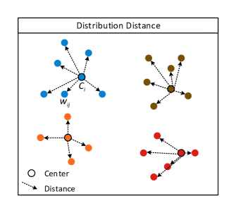
Figure 4: The distribution distance of kmeans++ cluster method.

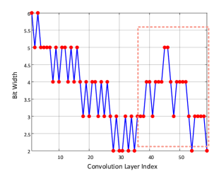
Figure 5: The bit width results of each convolution layer at the threshold $T=50$. The values of bit width progressively decrease with the deepening of the network layer. In addition, the bit width of the convolution layer before the detection module may be relevant large to maintaining more location discrimination information.

Take the distance threshold $T=50$ as an example, the Fig. 5 demonstrates the judgment results of bit width for each convolution layer. It can be indicated that the values of bit width progressively decrease with the deepening of the network layer. In addition, the bit width of the convolution layer before the detection process may be relevantly large to maintain more location discrimination information.

Algorithm 1 The Hybrid Quantization Method

1:The weights of $l^{th}$ certain convolution layer ${\bf{W}}\in\mathbb{R}{{}^{H\times W\times K\times K}}$, The manual distance threshold $T$ and the minimum bit width $b_{min}$

2:The bit width of the current convolution layer and activation $B_{l}$

3:Initialize the $B_{l}$ as 8

4:for $n$ in range ($b_{min}$,8) do

5:     Cluster weights into $2^{n}$ clusters via the kmeans++ algorithm and then get the centers $c_{i}$ and samples $w_{ij}$ of the $i^{th}$ cluster.

6:     Calculate the distribution distance according to Eq. 6.

7:     Update the bit width $B_{l}$ by Eq. 7

8:Complete the quantization for the convolution layer weight and activation by Eq. 9 and Eq. 10, respectively.

We use a simple-yet-effective quantization method which refers to [8] for both weights and activations. The uniform quantization function $q(\centerdot)$ is defined as:

$$q\left(v,k\right)=\frac{1}{{{2}^{k}}-1}round(({{2}^{k}}-1)v),$$ (8)

where $v$ is a real number indicating the full-precision (float32) value, $v\in[0,1]$. the output $q(v,k)$ of quantization function is a $k$ bits real number, $q(v,k)\in[0,1]$. The quantization calculations of $l_{th}$ convolution layer weight and activation are defined respectively as follows:

$${{w}^{l}_{o}}=2q(\frac{\tanh({{w}^{l}_{i}})}{2\max(\left|\tanh({{w}^{l}_{i}})\right|)}+\frac{1}{2},B^{l})-1,$$ (9)

$${{a}^{l}_{o}}=q({{a}^{l}_{i}},B^{l}).$$ (10)

The activation $a^{l}_{i}$ is the range in $[0,1]$ determined by a bounded activation function while the weight $w^{l}_{i}$ is not restricted in a limit boundary. Here, the quantization result of weight $w^{l}_{o}$ is the range in $[-1,1]$, and the quantization result of activation $a^{l}_{o}$ is the range in $[0,1]$. The Algorithm 1 clarifies the process of the hybrid quantization method. As described in [8], the first and last layers in the network are sensitive to performance during the process of quantization. Based on this intuition, the last detection layer keeps intact to avoid potential degradation of detection performance.

III-C One-to-one Self-teaching

Previous mixed quantization approaches pay more attention to the bit-width selection [7] which costs a lot of resources to obtain the optimal decision. Our hybrid quantization method can make a quick decision with less computation cost. The loss of performance is fixed by the guide of distillation. In general, previous distillation algorithms are a full precision network, so the network weights are in the same order of magnitude, and the feature maps generated by the teacher network or the student network are similar. However, for the quantitative network, the feature map generated by the quantitative network as a student network will have obvious weight information loss due to the increase of the zero content, resulting in some differences between the feature map of the teacher network and the feature map of the student network, which makes it difficult for the teacher network to directly restrict the quantitative student network from the feature layer. Therefore we proposed an OST to conquer this question. SCM first calculates the inner connected relationship between the full-precision and quantization network. The distillation switch (DS) chooses the core information between matched student and teacher features by this relationship matrix. We sketch the architecture of self-feature distillation in Fig. 2.

Let $\mathbf{s={s_{1},s_{2},...,s_{l}}}$ represent a set of multiscale feature maps for the student network and $\mathbf{t={t_{1},t_{2},...,t_{l}}}$ for the teacher. To calculate the attention map similar to [39] between the student feature and teacher feature, we define that each teacher feature generates a query $\bf{q_{i}}$, and each student feature produces a key $\bf{k_{j}}$:

$$\mathbf{q_{i}=W_{i}\cdot GAP(s_{i})},$$ (11)

$$\mathbf{k_{j}=W_{j}\cdot GAP(t_{j})}.$$ (12)

$\bf{GAP}(\cdot)$ represents a global average pooling. $\bf{W_{t}}$ and $\bf{W_{s}}$ are the liner transition parameters for the $i^{th}$ query and the $j^{th}$ key. Then the attention map that reveals the inner relationship between teacher and student features is defined as:

$$a=({{\bf{q}}\cdot{\bf{k^{T}}}})/\sqrt{d}.$$ (13)

Here, we introduce the Gumble-Softmax trick [43] to convert the values greater than the threshold to 1 and the rest to 0. Formally, the decision at $i^{th}$ entry of $a$ is derived in the following way:

$$\mathbf{A_{i,k}}=\frac{\exp({\log(\mathbf{a_{i,k}}+\mathbf{G_{i,k}})/\tau})}{\sum\limits_{j=1}^{K}{\exp}({\log(\mathbf{a_{i,j}}+\mathbf{G_{i,j}})/\tau})}\quad k=1,2,\ldots,K,$$ (14)

where K is set as $2$ for binary decision [44] in our case. $\bf G_{i}$ is the Gumbel distribution. Temperature $\tau$ is used to control the smoothness of $\bf A_{i}$. With a better attention map to mining the internal correlation of features, we generate a DS mask that can automatically determine whether to transfer the information from the teacher to the student at the same site in the network.

$$\alpha=\bf{Diag}(A).$$ (15)

where SCM digs out the diagonal elements from the attention map matrix $\bf A$. We devise the self-feature distillation loss as follows:

$$\mathcal{L}_{F}=\sum_{i=0}^{m}\alpha_{i}\|\bf{CAP}(t_{i})-\bf{CAP}(s_{i})\|_{2},$$ (16)

where $\bf{CAP}$ represents a channel-wise average pooling. $m$ is the total features utilized for distillation.

$$\mathcal{L}_{total}=\beta\mathcal{L}_{F}+\mathcal{L}_{dec},$$ (17)

Finally, the distillation loss terms are combined with detection loss and minimized in an end-to-end manner as Eq. 17. $\mathcal{L}_{dec}$ includes the objectness, location, and classification. The hyper-parameter $\beta$ indicates the impact balance between the detection and distillation.

IV Experimental Results

In this section, we evaluate the proposed method on the multimodal dataset for remote sensing object detection and four widely adopted CNNs with different scales. We first demonstrate the experience set up, including the introductions of datasets and networks, implementation details, and evaluation metrics. Then, we report the performance of our method on a dataset in detail, mean average precision and compression ratio are calculated to measure the comprehensive performance in the accuracy and computation cost.

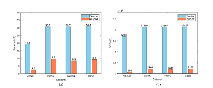
Figure 6: Comparisons of the teacher model and lightweight model by parameters and BOPs on the four datasets (VEDAI, DOTA, NWPU, and DIOR). The BOPs and parameters of the lightweight model are smaller, and the inference speed is faster. (a) Params (MB). (b) BOPs

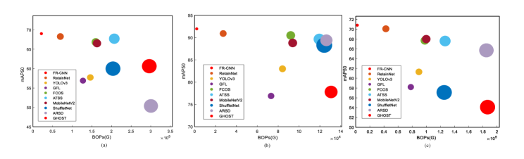
Figure 7: Comparison of the efficiency between the current SOTA methods and our method on the three datasets. The bigger size of cycles represents costing more parameters. (a) DOTA. (b) NWPU, and (c) DIOR.

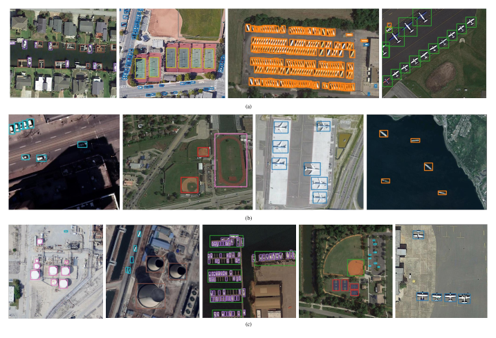
Figure 8: Three sets of visualization results. (a) DOTA. (b) NWPU, and (c) DIOR.

IV-A Dataset Description

The publicly available dataset VEDAI [45] designed for multimodal remote sensing image object detection is adopted in our experiments. In addition to validation on the multimodal object detection dataset, three single modal datasets (DOTA [46], NWPU [47] and DIOR [48]) are utilized in experiments to verify the generation of our proposed algorithm.

1) VEDAI: The VEDAI dataset consists of 1246 smaller images cropped from the much larger Utah Automated Geographic Reference Center (AGRC) dataset. Each image collected from the same altitude in AGRC has approximately $16,000\times 16,000$ pixels, with a resolution of about $12.5cm\times 12.5cm$ per pixel. The main scenes of VEDAI include grass, highway, mountains, and urban areas. The size of the image is fixed to $512\times 512$.

2) DOTA: The DOTA dataset was proposed by Xia et al. in 2018 for object detection of remote sensing. It contains 2806 large images and 188 282 instances, which are divided into 15 categories. The size of each original image is $4000\times 4000$, and the images are cropped into $1024\times 1024$ pixels with an overlap of 200 pixels in the experiment. We select half of the original images as the training set, 1/6 as the validation set, and 1/3 as the testing set. The size of the image is fixed to $512\times 512$.

3) NWPU VHR-10: The dataset of NWPU VHR-10 was proposed by Cheng et al. in 2016. It contains 800 images, of which 650 pictures contain objects, so we use 520 images as the training set and 130 images as the testing set. The dataset contains 10 categories, and the size of the image is fixed to $512\times 512$.

4) DIOR: The DIOR dataset was proposed by Li et al. in 2020 for the task of object detection, which involves 23 463 images and 192 472 instances. The size of each image is $800\times 800$. We choose 11 725 images as the training set and 11 738 images as the testing set.

TABLE I: Training Strategy

Dataset	Image Size	Batch Size	Lr	Epoch
VEDAI	512	2	0.01	300
DOTA	512	16	0.01	100
NWPU	512	8	0.01	150
DIOR	512	16	0.01	150

TABLE II: The comparison result of the tranditonal quantization method and our mixed-bit quantization and we use the same abbreviation in the following sections.

Bit Width	T	Max	Min	Car	Pickup	Camping	Truck	Other	Tractor	Boat	Van	mAP50	mAP	Params(MB)	BOPs(G)
32W32A	-	32	32	89.20	87.10	79.50	86.80	58.20	88.00	70.30	88.30	80.93	50.80	19.30	17023.76
8W8A	-	8	8	88.25	85.86	75.78	69.94	48.42	80.29	66.10	92.32	75.87	47.08	4.83	1201.10
HQ	0.1	7	8	86.58	83.06	69.90	76.45	69.77	76.75	69.77	99.51	79.57	48.55	4.34	1123.12
6W6A	-	6	6	86.81	87.16	69.77	75.72	61.58	81.99	60.46	83.87	75.92	45.63	3.63	727.04
HQ	4	3	8	90.94	86.57	74.45	73.35	55.92	79.70	68.63	97.84	78.42	46.32	2.49	691.88
4W4A	-	4	4	88.74	82.65	71.71	58.14	61.32	86.58	59.03	84.99	74.14	44.85	2.43	382.91
HQ	70	3	8	84.72	83.41	75.13	65.39	61.41	87.77	63.52	84.73	75.76	46.00	1.87	371.23

TABLE III: The validation result of the self-destillation method in the different model size.

HQ	T	Max	Min	OST	Car	Pickup	Camping	Truck	Other	Tractor	Boat	Van	mAP50	mAP
$\checkmark$	0.1	2	8		89.00	87.28	77.30	69.80	59.79	84.12	64.91	91.77	78.00	46.59
$\checkmark$	0.1	2	8	$\checkmark$	91.14	87.72	74.85	82.22	64.57	84.99	60.21	82.98	78.59	47.14
$\checkmark$	4	2	8		90.94	86.57	74.45	73.35	55.92	79.7	68.63	97.84	78.42	46.32
$\checkmark$	4	2	8	$\checkmark$	88.58	86.16	71.84	75.18	68.57	88.14	70.44	86.80	79.46	48.57
$\checkmark$	52	2	8		89.46	80.71	68.41	72.16	66.65	88.02	53.56	78.18	74.64	44.29
$\checkmark$	52	2	8	$\checkmark$	88.47	83.47	71.4	72.45	60.2	83.66	66.14	89.82	76.99	46.91

TABLE IV: The comparison with sota distillation method for detectors on the VEDAI .

Distillation	HQ	Car	Pickup	Camping	Truck	Other	Tractor	Boat	Van	mAP50	mAP
-	$\checkmark$	89.00	87.28	77.30	69.80	59.79	84.12	64.91	91.77	78.00	46.59
ZAQ [38]	$\checkmark$	88.04	85.86	70.51	79.45	45.16	88.14	67.76	84.03	76.12	46.48
AFD [39]	$\checkmark$	88.52	85.56	71.35	73.35	58.71	89.14	59.76	80.49	75.86	45.44
ReviewKD [40]	$\checkmark$	85.11	84.52	72.89	73.69	58.46	84.36	68.88	94.06	77.75	47.35
OST	$\checkmark$	91.14	87.72	74.85	82.22	64.57	84.99	60.21	82.98	78.59	47.14

TABLE V: mAP comparisons of different $\beta$ value.

	$\beta$	0	100	200	300	400	500
T	0.1	46.59	47.17	48.26	46.72	49.17	46.29
	4	46.32	48.57	47.05	47.96	47.29	49.05
	52	44.29	46.91	44.20	45.14	46.48	47.03

TABLE VI: Performance of different algorithms on VEDAI testing set.

Method	Car	Pickup	Camping	Truck	Other	Tractor	Boat	Van	mAP50	mAP	Params(MB)	BOPs(G)
YOLOv3	83.5	71.7	64.2	67.5	45.5	62.8	42.0	63.4	62.6	37.2	246	50,749
YOLOv4	86.2	70.9	71.9	75.3	54.9	69.3	30.7	66.6	65.7	40.9	210	39,076
YOLOv5s	81.1	71.3	70.8	66.4	58.1	67.3	27.0	55.7	62.2	34.6	28	5,427
YOLOv5m	81.6	73.9	59.0	70.0	57.2	77.7	30.5	65.5	64.4	38.2	84	16,599
YOLOv5l	84.3	76.8	74.0	75.0	51.5	61.3	30.3	57.4	63.9	37.9	186	37,530
YOLOv5x	84.7	66.4	66.8	72.4	65.8	67.2	29.2	58.8	63.9	37.8	349	71,301
Teacher	89.2	87.1	79.5	86.8	58.2	88.0	70.3	88.3	80.93	50.80	19.3	17,024
GHOST	88.82	86.06	74.33	86.96	61.28	86.00	71.76	87.26	80.31	49.05	2.5	692

TABLE VII: Performance of different algorithms on DOTA, NWPU and DIOR testing set.

	DOTA-v1.0			NWPU			DIOR
Method	mAP50	Params(MB)	BOPs(G)	mAP50	Params(MB)	BOPs(G)	mAP50	Params(MB)	BOPs(G)
Faster R-CNN	60.64	240	296,192	77.80	164	130,764	54.10	240	186,572
RetainNet	50.39	221	300,400	89.40	145	126,228	65.70	221	184,954
YOLOv3	60.00	246	203,694	88.30	246	124,180	57.10	247	125,153
GFL	66.53	76	163,000	88.80	76	93,931	68.00	76	99,768
FCOS	67.72	126	207,001	89.65	127	119,429	67.60	127	126,474
ATSS	66.84	75	159,754	90.50	75	92,057	67.70	75	97,792
MobileNetV2	56.91	41	127,221	76.90	41	73,205	58.20	41	77,926
ShuffleNet	57.73	48	146,022	83.00	48	84,142	61.30	48	89,405
O2-DNet	71.10	836	-	-	-	-	68.3	836	-
FMSSD	72.43	544	-	-	-	-	69.5	544	-
Teacher	71.65	203	291,491	93.21	127	122,234	71.7	203	178,176
ARSD	68.28 -3.37	52	69,662	90.92 -2.29	46	27,289	70.10 -1.6	52	42,598
Teacher	69.99	30.8	21,390	93.30	30.7	21,357	71.95	30.8	21,428
GHOST	69.02 -0.97	9.7	2,146	91.97 -1.33	8.5	1,927	71.53 -0.4	9.3	2158

IV-B Implementation Details

IV-B1 Networks

To demonstrate superior performance, SuperYOLO [41] is tested as a teacher model with our method. For the multimodal VEDAI dataset, the number of convolution layers is 47 including one detection layer on the small scale. For a single modal dataset (DOTA, NWPU, and DIOR), the number of convolution layers is 61 including three detection layers on the small, medium, and large scale. To verify the superiority of the GHOST proposed in this paper, we selected 12 generic methods for comparison:

one-stage algorithms (YOLOv3 [2], YOLOv4 [27], YOLOv5 [28], SuperYOLO, FCOS [4], ATSS [30], RetainNet [29], GFL [49]);

two-stage method (Faster R-CNN [3]);

lightweight models (MobileNetV2 [31] and ShuffleNet [32]);

distillation-based methods (ARSD [15]);

remote sensing designed approaches (FMSSD [50] and O2DNet [51]).

IV-B2 Training Strategy

Our proposed framework is implemented in PyTorch and runs on a workstation with an NVIDIA A100-SXM4-80GB GPU. We also use different training strategies for different datasets, and the detail is illustrated in TABLE I. In addition, data is augmented with Hue Saturation Value (HSV), multi-scale, translation, left-right flip, and mosaic. The augmentation strategy is canceled in the test stage. The standard Stochastic Gradient Descent (SGD) is used to train the network with a momentum of 0.937, weight decay of 0.0005 for the Nesterov accelerated gradients utilized, and a batch size of 2. The learning rate is set to 0.01 initially. All the baseline training process is completed from scratch without any pre-trained model while the GHOST is carried on the baseline model. In the test stage, the IoU threshold of non-maximum suppression is 0.6 on NWPU VHR-10 and VEDAI, and it is 0.4 on DOTA and DIOR.

IV-B3 Evaluation Metric

For the detection result, the IoU is defined as the ratio of the intersection and union of two boxes. During the evaluation, according to the IoU of predicted boxes and ground truths, each sample will be assigned attributes: true positive (TP) for correctly matching, false positive (FP) for wrongly predicting the background as an object, and false negative (FN) for the undetected object. During the evaluation, all the detection boxes are sorted in order of confidence score from high two low and then traversed. In the traversed process, the calculations of the precision and recall metrics can be defined as:

$$Precision=\frac{TP}{TP+FP},$$ (18)

$$Recall=\frac{TP}{TP+FN}.$$ (19)

The precision and recall are correlated with the commission and omission errors, respectively. The AP values use an integral method to calculate the area enclosed by the Precision-Recall curve and coordinate axis of all categories. Hence, the AP can be calculated by

$$AP=\int_{0}^{1}{p(r)dr},$$ (20)

where $p$ denotes Precision, $r$ denotes Recall. The mAP is a comprehensive indicator obtained by averaging APs for all classes. Moreover, we choose Bit-Operations (BOPs) count [52] and parameters to measure the compression performance. The Bops of convolution are calculated as:

$$BOPs_{l}=c_{l-1}\times c_{l}\times w_{l}\times h_{l}\times k_{w}\times k_{h}\times b_{w,l}\times b_{a,l-1}.$$ (21)

The $h_{l}$, $w_{l}$, and $c_{l}$ are the with, height, and several channels of the $l-th$ layer output feature map, respectively. $b_{w,l}$ and $b_{a,l}$ denote $l-th$ layer weight and activation bit-weight. The parameters (params) are defined as:

$$params=\frac{c_{l-1}\times c_{l}\times k_{h}\times k_{w}\times b_{w,l}}{8bit}(B).$$ (22)

IV-C Ablation Study

In this section, we conduct the ablation experiments of our GHOST framework. We explore how each module (HQ and OST) compresses the model and promotes the performance of the small student model. Besides, the experiments of different distillation algorithms and distillation hyperparameters’ optimization are carried out. We conduct ablation experiments on the dataset of VEDAI for object detection.

Validation of HQ: Distribution distance hybrid quantization can integrate device n-bit settings for the network, so we experiment with such variations of integrated hybrid n-bit quantization. To analyze the performance of differences, we compare fixed DoReFa-Net [8] and various hybrid DoReFa-Net quantization methods on the SuperYOLO detection network. As illustrated in TABLE II, the HQ is the proposed hybrid quantization method, and the $\cdot W\cdot A$ presents the traditional unified bit width quantization algorithm except $32W32A$ represents the full precision network. Max and Min denote the maximum and minimum bit width in the quantization model. Hybrid quantization enables the quantization model to preserve the significant information to achieve the minimal accuracy loss possible. As shown in TABLE II, the hybrid quantization module accomplishes the optimal consequence and detection accuracy has reached $79.57\%$, $78.42\%$, and $75.76\%$ respectively, which are more $3.7\%$, $2.5\%$, and $1.62\%$ than fixed quantization at the different computation orders. The hybrid quantization achieves better accuracy in the VEDAI dataset than the accuracy of fixed quantization costing fewer computation resources (parameters and BOPs).

Effect of OST Module: After the HQ module has been added to the network, we also adopt one-to-one self-teaching within the three-quantization scale. Table III is based on SuperYOLO which is used as the teacher network and student network simultaneously. The experiments are carried out on the VEDAI dataset. The OST module enables the typical detection network to recover the performance of the quantization detection network improved by $0.59\%$, $1.04\%$, and $2.35\%$, respectively no matter what kind of bit width.

Comparison with the SOTA Distillation Method: In addition, Table IV shows the comparisons between the proposed OST module and existing distillation frameworks. OST achieves superior performance in the field of remote sensing under the premise of the same computation cost while the ZAQ, AFD, and ReviewKD lead to an accuracy degradation of the quantization network. And also it can be proved that OST distillation is a benefit for the guidance between the full-precision model and the quantization model.

Hyperparameters Optimization: As presented in Section III-C, $\beta$ is the distillation weights of the OST module, so we compare the performance of the distillation in the different weights which are shown in TABLE V. We conduct the hyperparameter experiment on the VEDAI dataset on GHOST to find the best $\beta$. As shown in the TABLE V shows, the model reaches the best when $\beta=400$ at the $T=0.1$ and when $\beta=400$ at the $T=4$ or $T=52$.

Lightweight Analysis: Owning to the GQSD design idea, our student model is very lightweight. We compare the GHOST and the teacher model in terms of parameters and BOPs on the four datasets. As Fig. 6 shows, GHOST has smaller model parameters, and fewer BOPs compared with the teacher model no matter in which dataset. Hence, our compression strategy for the lightweight model is more practical to be deployed on intelligent terminals.

IV-D Comparison with the SOTA Detectors

In this part, we compare our lightweight model with other classic heavy object detection methods. As shown in TABLE VI and TABLE VII. Experiments on the four datasets prove the efficiency and efficacy of the GHOST framework. Not only does our lightweight have higher accuracy but also it has strong information retention capability under extreme model compression.

1) VEDAI: Our GHOST achieves 80.31% mAP50 compared with other detectors, surpassing the one-stage series mentioned in TABLE VI. Our model achieves the lowest model parameters (2.5 MB) and BOPs (692 G).

2) DOTA: As presented in TABLE VII, our GHOST achieves the optimal detection result (69.02% mAP50) and the model parameters (9.7 MB) and BOPs (2,146 G) are much smaller than other SOTA detectors regardless of the two-stage, one-stage, anchor-free or distillation-based method. We also compare two detectors designed for remote sensing imagery such as FMSSD [50] and O2DNet [51]. Although these models have a close performance with our lightweight model, the huger parameters and BOPs seem to be a massive cost in computation resources. Hence, our model has a better balance in consideration of detection efficiency and efficacy. Compare to the distillation-based method ARSD (-3.37%), the GHOST obtains an even smaller accuracy gap (-0.97%) between the student network and the teacher network. It demonstrates that our GHOST method can transfer sufficient knowledge to guide the learning of the student model and the misunderstanding between both models can be reduced by the SCM training strategy.

3) NWPU: We compare the results of our method with other approaches on the NWPU dataset. As shown in TABLE VII, our GHOST obtains the best result (91.97% mAP50) with the smallest amount of model parameters (8.5 MB) and the fewer BOPs (1,927 G).

4) DIOR: As illustrated in TABLE VII, our GHOST achieves the optimal detection result (69.02% mAP50) and the model parameters (9.3 MB) and BOPs (2,158 G) are much smaller than other SOTA detectors regardless of the two-stage, one-stage, anchor-free lightweight, distillation-based methods. It reveals the strong ability to compress models and the power capacity of object detection in remote sensing imagery. The accuracy of the student GHOST is only a bit less 0.4% than teacher network, compared with ARSD (1.6%).

In order to show the performance of our algorithm more intuitively, We compare the detection accuracy, parameters, and BOPs of various algorithms in Fig. 7. It can be obvious that GHOST has a better trade-off between performance and lightweight. The visualization results on the three datasets are illustrated in Fig. 8 in which we can see that the GHOST can have an outstanding detection of objects at different scales.

V Conclusion

In this paper, we propose a GHOST framework for a lightweight object detection method in remote sensing imagery. We first design a guided quantization self-distillation structure which is not only a training technique to preserve model performance but also a method to compress and accelerate models. Although most of the previous research focuses on knowledge transfer among different models, we believe that inside distillation is also very promising. Secondly, we propose a hybrid quantization that captures the optimal bit width selection based on an adaptive way in the weight value research space to break the limit of the fixed quantization model accuracy. Thirdly, the proposed one-to-one self-teaching module gives the student network of self-judgment through a switch control machine that accurately handles the knowledge transformation. It can dynamically discriminate the wrong guidance and mine the effective knowledge from the teacher. The experiments based on the VEDAI, DOTA, NWPU, and DIOR datasets certify that our GHOST achieves SOTA performance compared with other detectors. It can well balance the tradeoff between accuracy and specific resource constraints.

References

- [1] J. Ding, N. Xue, Y. Long, G.-S. Xia, and Q. Lu, “Learning roi transformer for oriented object detection in aerial images,” in Proc. IEEE Conf. Comput. Vis. Pattern Recognit. (CVPR), 2019, pp. 2844–2853.
- [2] J. Redmon and A. Farhadi, “YOLOv3: An incremental improvement,” arXiv, 2018. [Online]. Available: https://arxiv.org/abs/1804.02767
- [3] S. Ren, K. He, R. Girshick, and J. Sun, “Faster r-cnn: Towards real-time object detection with region proposal networks,” Proc. Adv. Neural Inf. Process. Syst., vol. 28, 2015.
- [4] Z. Tian, C. Shen, H. Chen, and T. He, “Fcos: Fully convolutional one-stage object detection,” in Proc. IEEE Int. Conf. Comput. Vis., 2019, pp. 9627–9636.
- [5] J.-H. Luo and J. Wu, “Neural network pruning with residual-connections and limited-data,” in Proc. IEEE Conf. Comput. Vis. Pattern Recognit. (CVPR), 2020, pp. 1455–1464.
- [6] R. Li, Y. Wang, F. Liang, H. Qin, J. Yan, and R. Fan, “Fully quantized network for object detection,” in Proc. IEEE Conf. Comput. Vis. Pattern Recognit. (CVPR), 2019, pp. 2810–2819.
- [7] Z. Wang, H. Xiao, J. Lu, and J. Zhou, “Generalizable mixed-precision quantization via attribution rank preservation,” in Proc. IEEE Int. Conf. Comput. Vis., 2021, pp. 5291–5300.
- [8] S. Zhou, Y. Wu, Z. Ni, X. Zhou, H. Wen, and Y. Zou, “Dorefa-net: Training low bitwidth convolutional neural networks with low bitwidth gradients,” arXiv preprint arXiv:1606.06160, 2016.
- [9] G.-H. Wang, Y. Ge, and J. Wu, “Distilling knowledge by mimicking features,” IEEE Trans. Pattern Anal. Mach. Intell., 2021.
- [10] X. Dai, Z. Jiang, Z. Wu, Y. Bao, Z. Wang, S. Liu, and E. Zhou, “General instance distillation for object detection,” in Proc. IEEE Conf. Comput. Vis. Pattern Recognit. (CVPR), 2021, pp. 7842–7851.
- [11] H. Yang, L. Duan, Y. Chen, and H. Li, “Bsq: Exploring bit-level sparsity for mixed-precision neural network quantization,” arXiv preprint arXiv:2102.10462, 2021.
- [12] Z. Liu, Z. Shen, M. Savvides, and K.-T. Cheng, “Reactnet: Towards precise binary neural network with generalized activation functions,” in Proc. Eur. Conf. Comput. Vis. Springer, 2020, pp. 143–159.
- [13] G. Hinton, O. Vinyals, J. Dean et al., “Distilling the knowledge in a neural network,” arXiv preprint arXiv:1503.02531, vol. 2, no. 7, 2015.
- [14] J. Gou, B. Yu, S. J. Maybank, and D. Tao, “Knowledge distillation: A survey,” Int. J. Comput. Vis., vol. 129, no. 6, pp. 1789–1819, 2021.
- [15] Y. Yang, X. Sun, W. Diao, H. Li, Y. Wu, X. Li, and K. Fu, “Adaptive knowledge distillation for lightweight remote sensing object detectors optimizing,” IEEE Trans. on Geosci. and Remote Sens., 2022.
- [16] L. Zhang, J. Song, A. Gao, J. Chen, and K. Ma, “Be your own teacher: Improve the performance of convolutional neural networks via self distillation,” in Proc. IEEE Int. Conf. Comput. Vis., 2019.
- [17] M. Ji, S. Shin, S. Hwang, G. Park, and I.-C. Moon, “Refine myself by teaching myself: Feature refinement via self-knowledge distillation,” in Proc. IEEE Conf. Comput. Vis. Pattern Recognit. (CVPR), 2021, pp. 10 664–10 673.
- [18] Y. Hou, Z. Ma, C. Liu, and C. C. Loy, “Learning lightweight lane detection cnns by self attention distillation,” in Proc. IEEE Int. Conf. Comput. Vis., 2019, pp. 1013–1021.
- [19] J. R. R. Uijlings, K. E. A. Van De Sande, T. Gevers, and A. W. M. Smeulders, “Selective search for object recognition,” Int. J. Comput. Vis., vol. 104, no. 2, pp. 154–171, 2013.
- [20] R. Girshick, D. Jeff, D. Trevor, and M. Jitendra, “Rich feature hierarchies for accurate object detection and semantic segmentation,” in Proc. IEEE Conf. Comput. Vis. Pattern Recognit. (CVPR), 2014, pp. 580–587.
- [21] R. Girshick, “Fast r-cnn,” in Proc. IEEE Int. Conf. Comput. Vis., 2015, pp. 1440–1448.
- [22] W. Liu, D. Anguelov, D. Erhan, C. Szegedy, S. Reed, C.-Y. Fu, and A. C. Berg, “SSD: Single shot multibox detector,” in Proc. Eur. Conf. Comput. Vis. Springer, 2016, pp. 21–37.
- [23] C.-Y. Fu, W. Liu, A. Ranga, A. Tyagi, and A. C. Berg, “DSSD: Deconvolutional single shot detector,” arXiv preprint arXiv:1701.06659, 2017.
- [24] L. Cui, R. Ma, P. Lv, X. Jiang, Z. Gao, B. Zhou, and M. Xu, “MDSSD: multi-scale deconvolutional single shot detector for small objects,” arXiv preprint arXiv:1805.07009, 2018.
- [25] J. Redmon, S. Divvala, R. Girshick, and A. Farhadi, “You only look once: Unified, real-time object detection,” in Proc. IEEE Conf. Comput. Vis. Pattern Recognit. (CVPR), 2016, pp. 779–788.
- [26] J. Redmon and A. Farhadi, “Yolo9000: better, faster, stronger,” in Proc. IEEE Conf. Comput. Vis. Pattern Recognit. (CVPR), 2017, pp. 7263–7271.
- [27] A. Bochkovskiy, C. Wang, and H. M. Liao, “YOLOv4: Optimal speed and accuracy of object detection,” arXiv, 2020. [Online]. Available: https://arxiv.org/abs/2004.10934v1
- [28] G. J. et al., “ultralytics/yolov5: v5.0,” 2021. [Online]. Available: https://github.com/ultralytics/yolov5
- [29] T.-Y. Lin, P. Goyal, R. Girshick, K. He, and P. Dollár, “Focal loss for dense object detection,” in Proc. IEEE Int. Conf. Comput. Vis., 2017, pp. 2980–2988.
- [30] S. Zhang, C. Chi, Y. Yao, Z. Lei, and S. Z. Li, “Bridging the gap between anchor-based and anchor-free detection via adaptive training sample selection,” in Proc. IEEE Conf. Comput. Vis. Pattern Recognit. (CVPR), 2020, pp. 9759–9768.
- [31] M. Sandler, A. Howard, M. Zhu, A. Zhmoginov, and L.-C. Chen, “Mobilenetv2: Inverted residuals and linear bottlenecks,” in Proc. IEEE Conf. Comput. Vis. Pattern Recognit. (CVPR), 2018, pp. 4510–4520.
- [32] X. Zhang, X. Zhou, M. Lin, and J. Sun, “Shufflenet: An extremely efficient convolutional neural network for mobile devices,” in Proc. IEEE Conf. Comput. Vis. Pattern Recognit. (CVPR), 2018, pp. 6848–6856.
- [33] F. N. Iandola, S. Han, M. W. Moskewicz, K. Ashraf, W. J. Dally, and K. Keutzer, “Squeezenet: Alexnet-level accuracy with 50x fewer parameters and <0.5 mb model size,” arXiv preprint arXiv:1602.07360, 2016.
- [34] B. Zhao, Q. Cui, R. Song, Y. Qiu, and J. Liang, “Decoupled knowledge distillation,” arXiv preprint arXiv:2203.08679, 2022.
- [35] Y. Zhang, Z. Yan, X. Sun, W. Diao, K. Fu, and L. Wang, “Learning efficient and accurate detectors with dynamic knowledge distillation in remote sensing imagery,” IEEE Trans. on Geosci. and Remote Sens., 2021.
- [36] Y. Cai, Z. Yao, Z. Dong, A. Gholami, M. W. Mahoney, and K. Keutzer, “Zeroq: A novel zero shot quantization framework,” in Proc. IEEE Conf. Comput. Vis. Pattern Recognit. (CVPR), 2020, pp. 13 169–13 178.
- [37] Z. Dong, Z. Yao, D. Arfeen, A. Gholami, M. W. Mahoney, and K. Keutzer, “Hawq-v2: Hessian aware trace-weighted quantization of neural networks,” Proc. Adv. Neural Inf. Process. Syst., vol. 33, pp. 18 518–18 529, 2020.
- [38] Y. Liu, W. Zhang, and J. Wang, “Zero-shot adversarial quantization,” in Proc. IEEE Conf. Comput. Vis. Pattern Recognit. (CVPR), 2021, pp. 1512–1521.
- [39] M. Ji, B. Heo, and S. Park, “Show, attend and distill: Knowledge distillation via attention-based feature matching,” in Proc. AAAI Conf. Artif. Intell., vol. 35, no. 9, 2021, pp. 7945–7952.
- [40] P. Chen, S. Liu, H. Zhao, and J. Jia, “Distilling knowledge via knowledge review,” in Proc. IEEE Conf. Comput. Vis. Pattern Recognit. (CVPR), 2021, pp. 5008–5017.
- [41] J. Zhang, J. Lei, W. Xie, Z. Fang, Y. Li, and Q. Du, “Superyolo: Super resolution assisted object detection in multimodal remote sensing imagery,” arXiv preprint arXiv:2209.13351, 2022.
- [42] L. Van der Maaten and G. Hinton, “Visualizing data using t-sne,” J. Mach. Learn. Res., vol. 9, no. 11, 2008.
- [43] I. Ng, S. Zhu, Z. Fang, H. Li, Z. Chen, and J. Wang, “Masked gradient-based causal structure learning,” in Proc. SIAM Int. Conf. Data Min. (SDM). SIAM, 2022, pp. 424–432.
- [44] L. Meng, H. Li, B.-C. Chen, S. Lan, Z. Wu, Y.-G. Jiang, and S.-N. Lim, “Adavit: Adaptive vision transformers for efficient image recognition,” in Proc. IEEE Conf. Comput. Vis. Pattern Recognit. (CVPR), 2022, pp. 12 309–12 318.
- [45] S. Razakarivony and F. Jurie, “Vehicle detection in aerial imagery: A small target detection benchmark,” J. Vis. Commun. Image Represent., vol. 34, pp. 187–203, 2016.
- [46] G.-S. Xia, X. Bai, J. Ding, Z. Zhu, S. Belongie, J. Luo, M. Datcu, M. Pelillo, and L. Zhang, “Dota: A large-scale dataset for object detection in aerial images,” in Proc. IEEE Conf. Comput. Vis. Pattern Recognit. (CVPR), 2018, pp. 3974–3983.
- [47] G. Cheng, P. Zhou, and J. Han, “Learning rotation-invariant convolutional neural networks for object detection in vhr optical remote sensing images,” IEEE Trans. on Geosci. and Remote Sens., vol. 54, no. 12, pp. 7405–7415, 2016.
- [48] K. Li, G. Wan, G. Cheng, L. Meng, and J. Han, “Object detection in optical remote sensing images: A survey and a new benchmark,” ISPRS J. Photogramm. Remote Sens., vol. 159, pp. 296–307, 2020.
- [49] X. Li, W. Wang, L. Wu, S. Chen, X. Hu, J. Li, J. Tang, and J. Yang, “Generalized focal loss: Learning qualified and distributed bounding boxes for dense object detection,” Proc. Adv. Neural Inf. Process. Syst., vol. 33, pp. 21 002–21 012, 2020.
- [50] P. Wang, X. Sun, W. Diao, and K. Fu, “Fmssd: Feature-merged single-shot detection for multiscale objects in large-scale remote sensing imagery,” IEEE Trans. on Geosci. and Remote Sens., vol. 58, no. 5, pp. 3377–3390, 2020.
- [51] H. Wei, Y. Zhang, Z. Chang, H. Li, H. Wang, and X. Sun, “Oriented objects as pairs of middle lines,” ISPRS J. Photogramm. Remote Sens., vol. 169, pp. 268–279, 2020.
- [52] Y. Wang, Y. Lu, and T. Blankevoort, “Differentiable joint pruning and quantization for hardware efficiency,” in Proc. Eur. Conf. Comput. Vis. Springer, 2020, pp. 259–277.