Accuracy-Guaranteed Collaborative DNN Inference in Industrial IoT via Deep Reinforcement Learning

Abstract

Collaboration among industrial Internet of Things (IoT) devices and edge networks is essential to support computation-intensive deep neural network (DNN) inference services which require low delay and high accuracy. Sampling rate adaption which dynamically configures the sampling rates of industrial IoT devices according to network conditions, is the key in minimizing the service delay. In this paper, we investigate the collaborative DNN inference problem in industrial IoT networks. To capture the channel variation and task arrival randomness, we formulate the problem as a constrained Markov decision process (CMDP). Specifically, sampling rate adaption, inference task offloading and edge computing resource allocation are jointly considered to minimize the average service delay while guaranteeing the long-term accuracy requirements of different inference services. Since CMDP cannot be directly solved by general reinforcement learning (RL) algorithms due to the intractable long-term constraints, we first transform the CMDP into an MDP by leveraging the Lyapunov optimization technique. Then, a deep RL-based algorithm is proposed to solve the MDP. To expedite the training process, an optimization subroutine is embedded in the proposed algorithm to directly obtain the optimal edge computing resource allocation. Extensive simulation results are provided to demonstrate that the proposed RL-based algorithm can significantly reduce the average service delay while preserving long-term inference accuracy with a high probability.

I Introduction

With the development of advanced neural network techniques and ubiquitous industrial Internet of Things (IoT) devices, deep neural network (DNN) is widely applied in extensive industrial IoT applications, such as facility monitoring and fault diagnosis [1]. Industrial IoT devices (e.g., vibration sensors) can sense the industrial operating environment and feed sensing data to a DNN, and then the DNN processes the sensing data and renders inference results, namely DNN inference. Although DNN inference can achieve high inference accuracy as compared to traditional alternatives (e.g., decision tree), executing DNN inference tasks requires extensive computation resource due to tremendous multiply-and-accumulation operations [2]. A device-only solution that purely executes DNN inference tasks at resource-constrained industrial IoT devices, becomes intractable due to prohibitive energy consumption and a high service delay. For example, processing an image using AlexNet incurs up to 0.45 W energy consumption [3]. An edge-only solution which purely offloads large-volume sensing data to resource-rich edge nodes, e.g., access point (AP), suffers from an unpredictable service delay due to time-varying wireless channel [4]. Hence, neither a device-only nor an edge-only solution can effectively support low-delay DNN inference services.

Collaborative inference, which coordinates resource-constrained industrial IoT devices and the resource-rich AP, becomes a de-facto paradigm to provide low-delay and high-accuracy inference services [5]. Within the collaborative inference, sensing data from industrial IoT devices can be either processed locally or offloaded to the AP. At industrial IoT devices, light-weight compressed DNNs (i.e., neural networks are compressed without significantly decreasing their performance) are deployed due to constrained on-board computing capability, which saves computing resource at the cost of inference accuracy [6, 7]. At the AP, uncompressed DNNs are deployed to provide high-accuracy inference services at the cost of network resources. Through the resource allocation (e.g., task offloading) between industrial IoT devices and the AP, the overall service performance can be enhanced.

However, the sampling rate adaption technique that dynamically configures the sampling rates of industrial IoT devices, is seldom considered. Through dynamically adjusting the sampling rates according to channel conditions and AP’s workload, sensing data from industrial IoT devices can be compressed, thereby reducing not only the offloaded data volume, but also task computation workload. In our experiments, we implement AlexNet to conduct bearing fault diagnosis based on the collected bearing vibration signal from dataset [8]. As shown in Fig. 1, inference accuracy grows sub-linearly with the sampling rate. For example, when the sampling rate increases from 18 KHz to 24 KHz, the accuracy increases from 95% to 98.7%. Hence, when the channel condition is poor or edge computation workload is heavy, decreasing the sampling rate can reduce the offloaded data volume and requested computation workload, thereby reducing the service delay at the cost of limited inference accuracy. When channel condition is good and edge computation workload is light, increasing the sampling rate can help deliver a high-accuracy service with an acceptable service delay. Hence, sampling rate adaption can effectively reduce the service delay, which should be incorporated in the collaborative DNN inference.

The sampling rate adaption and resource allocation for collaborative DNN inference are entangled with the following challenges. Firstly, due to time-varying channel conditions and random task arrivals, sampling rate and resource allocation should be dynamically adjusted to achieve the minimum service delay. Minimizing the long-term service delay requires the stochastic information of network dynamics. Secondly, in addition to minimizing the service delay, the long-term accuracy requirements should be guaranteed for different inference services. The long-term accuracy performance is determined by decisions of sampling rate adaption and resource allocation over time, and hence the optimal decisions require future network information. To address the above two challenges, a reinforcement learning (RL) technique is leveraged to interact with the unknown environment to capture the network dynamics, and then a Lyapunov optimization technique is utilized within the RL framework to guarantee the long-term accuracy requirements without requiring future network information.

In this paper, we investigate the collaborative DNN inference problem in industrial IoT networks. Firstly, we formulate the problem as a constrained Markov decision process (CMDP) to account for time-varying channel conditions and random task arrivals. Specifically, sampling rates of industrial IoT devices, task offloading, and edge computation resource allocation are optimized to minimize the average service delay while guaranteeing the long-term accuracy requirements of multiple services. Secondly, since traditional RL algorithms target at optimizing a long-term reward without considering policy constraints, they cannot be applied to solve CMDP with long-term constraints. To solve the problem, we transform the CDMP into an MDP via the Lyapunov optimization technique. The core idea is to construct accuracy deficit queues to characterize the satisfaction status of the long-term accuracy constraints, thereby guiding the learning agent to meet the long-term accuracy constraints. Thirdly, to solve the MDP, a learning-based algorithm is developed based on the deep deterministic policy gradient (DDPG) algorithm. Within the learning algorithm, to reduce the training complexity, edge computing resource allocation is directly solved via an optimization subroutine based on convex optimization theory, since it only impacts one-shot delay performance according to theoretical analysis. Extensive simulations are conducted to validate the effectiveness of the proposed algorithm in reducing the average service delay while preserving the long-term accuracy requirements.

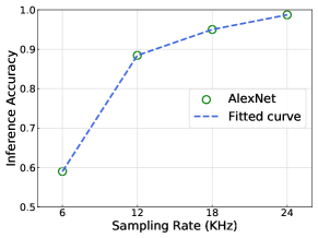
Fig. 1: Inference accuracy with respect to sampling rates on the bearing vibration dataset [8].

Our main contributions in this paper are summarized as follows:

• We formulate the collaborative DNN inference problem as a CMDP, in which the objective is to minimize the average service delay while guaranteeing the long-term accuracy constraints;

• We transform the CMDP into an MDP via the Lyapunov optimization technique which constructs accuracy deficit queue to characterize the satisfaction status of the long-term accuracy constraints;

• We propose a deep RL-based algorithm to make the optimal sampling rate adaption and resource allocation decisions. To reduce the training complexity, an optimization subroutine is embedded in the proposed algorithm for the optimal edge computing resource allocation.

The remainder of this paper is organized as follows. Section II reviews related works. The system model and problem formulation are presented in Section III. Section IV proposes a learning-based solution. Simulation results are given in Section V. Finally, Section VI concludes this paper.

II Related Work

DNN inference for resource-constrained industrial IoT devices has garnered much attention recently. A device-only solution aims to facilitate DNN inference services resorting to on-board computing resources. To reduce the computational complexity, DNN compression techniques are applied, such as weight pruning [6] and knowledge distillation [9]. Considering the widely-equipped energy-harvesting functionality in IoT devices, Gobieski et al. designed a light-weight DNN inference model, which can dynamically compress the model size in order to balance inference accuracy and energy efficiency [2]. In another line of research, edge-assisted DNN inference solutions can provide high-accuracy inference services by utilizing powerful edge computing servers. To facilitate low-delay and accurate DNN-based video analytics, Yang et al. proposed an online video quality and computing resource allocation strategy to maximize video analytic accuracy [10]. Another inspiring work proposed a novel device-edge collaborative inference scheme, in which the DNN model is partitioned and deployed at both the device and the edge, and intermediate results are transferred via wireless links [5]. The above works can provide possible resource allocation solutions to enhance DNN inference performance. Different from existing works, our work takes the sampling rate adaption of industrial IoT devices into account, aiming at providing accuracy-guaranteed inference services in dynamic industrial IoT networks.

RL algorithms have been widely applied in allocating network resources in wireless networks, such as service migration in vehicular networks [11], network slicing in cellular networks [12], content caching in edge networks [13], and task scheduling in industrial IoT networks [14]. Hence, RL algorithms are considered as plausible solutions to manage network resources for DNN inference services. However, DNN inference services require minimizing the average delay while satisfying the long-term accuracy constraints. Traditional RL algorithms, e.g., DDPG, can be applied to solve MDPs, in which learning agents seek to optimize a long-term reward without policy constraints, while they cannot deal with constrained long-term optimization problems [15, 16]. Our proposed deep RL-based algorithm can address long-term constraints within the RL framework by the modification of reward based on the Lyapunov optimization technique. In addition, an optimization subroutine is embedded in our algorithm to further reduce the training complexity.

III System Model and Problem Formulation

III-A Network Model

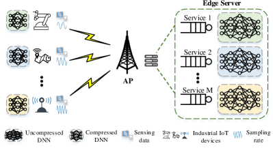
Fig. 2: The collaborative DNN inference framework for industrial IoT devices.

As shown in Fig. 2, we consider a wireless network with one AP to serve multiple types of industrial IoT devices. The AP is in charge of collecting network information and resource orchestration within the network. Consider $M$ types of inference services, denoted by a set $\mathcal{M}$, such as facility fault diagnosis and facility monitoring services. Taking the facility fault diagnosis service as an example, vibration sensors installed on industrial IoT devices sense the operating conditions at a sampling rate, and feed the sensed vibration signal into a DNN, then the DNN diagnoses the facility fault type. The set of industrial IoT devices subscribed to service $m$ is denoted by $\mathcal{N}_{m}$, and the set of all industrial IoT devices is denoted by $\mathcal{N}=\cup_{m\in\mathcal{M}}\mathcal{N}_{m}$. In the collaborative inference framework, two types of DNNs are deployed. One is a compressed DNN, which is deployed at industrial IoT devices. The compressed DNN can be implemented via the weight pruning technique, which prunes less-important weights to reduce computational complexity while maintaining similar inference accuracy [6]. The other is an uncompressed DNN, which is deployed at the AP. In this way, $M$ types of uncompressed DNNs share the edge computing resource to serve different inference requests. Important notations are summarized in Table I.

The collaborative DNN inference framework operates in a time-slotted manner. Let $t$ denote the time index, where $t\in\mathcal{T}=\{1,2,...,T\}$. The detailed procedure is given as follows.

1. Sampling rate selection: Industrial IoT devices first select their sampling rates according to channel conditions and computation workloads. The set of candidate sampling rates is denoted by $\mathcal{K}=\{\theta_{1},\theta_{2},...,\theta_{K}\}$, where $\theta_{K}$ denotes the raw sampling rate. We assume the sampling rate in $\mathcal{K}$ increases linearly with the index, i.e., $\theta_{k}=k\theta_{K}/{K}$. Let $\mathbf{X}^{t}$ denote the sampling rate decision matrix in time slot $t$, whose element $x_{n,k}^{t}=1$ indicates industrial IoT device $n\in\mathcal{N}$ selects the $k$-th sampling rate.

2. Task processing: The sensing data from industrial IoT devices within a time slot is deemed as a computation task, which can be either offloaded to the AP or executed locally. Let $\mathbf{o}^{t}\in\mathbb{R}^{|\mathcal{N}|\times 1}$ denote the offloading decision vector in time slot $t$, whose element $o_{n}^{t}=0$ indicates offloading the computation task from industrial IoT device $n$. Otherwise, $o_{n}^{t}=1$ indicates executing the computation task locally.

Table I: Summary of notations.

Notation	Description
$A_{m}$	Achieved instantaneous accuracy of service $m$
$A_{m}^{th}$	Long-term accuracy requirement of service $m$
$B^{t}$	Local computing queue backlog in time slot $t$
$\mathbf{c}$	Computing resource allocation decision vector
$D$	Service delay
$L\left(\cdot\right)$	Lyapunov function
$\mathbf{o}$	Task offloading decision vector
$Q^{t}$	Edge computing queue backlog in time slot $t$
$V$	Parameter to balance delay and accuracy requirement
$\mathbf{X}$	Sampling rate selection decision matrix of all devices
$Z^{t}$	Accuracy deficit queue backlog in time slot $t$
$\xi_{n}$	Raw task data size of device $n$
$\eta_{m}$	Task computation intensity of service $m$
$\lambda_{n}$	Average task arrival rate of device $n$
$\zeta\left(\mathbf{x}_{n}^{t}\right)$	Task data size of device $n$ in time slot $t$
$\Psi^{t}$	Amount of dropped tasks in computing queues

III-B Service Delay Model

A computation task can be either processed locally or offloaded to the AP. In what follows, we analyze the service delay in these two cases.

III-B1 Executing locally

Let $\lambda_{n}^{t}$ denote the task arrival rate of the $n$-th industrial IoT device in time slot $t$, which is assumed to follow a general random distribution. The raw data size of the generated tasks at the $n$-th device is denoted by $\xi_{n}^{t}=\lambda_{n}^{t}\nu_{m},\forall n\in\mathcal{N}_{m}$, where $\nu_{m}$ denotes the raw data size of a task for service $m$. After the sampling rate is selected, the data size of the generated task is represented by $\zeta\left(\mathbf{x}_{n}^{t}\right)=\sum_{k=1}^{K}x_{n,k}^{t}\xi_{n}^{t}k/K$, where $\mathbf{x}_{n}^{t}=\{x_{n,k}^{t}\}_{k\in\mathcal{K}}$ is the sampling rate selection decision vector of the $n$-th device. When the inference task is processed locally by a compressed DNN, the service delay includes the queuing delay in the local computing queue and task processing delay, which is given by

$$d^{t}_{n,l}=\frac{o_{n}^{t}\eta_{m,c}\left(B_{n}^{t}+\zeta\left(\mathbf{x}_{n}^{t}\right)\right)}{f_{n}},\forall n\in\mathcal{N}_{m},$$ (1)

where $f_{n}$ is the CPU frequency of the $n$-th industrial IoT device, and $\eta_{m,c}$ denotes the computation intensity of the compressed DNN for the $m$-th service. Here, $B_{n}^{t}$ is the backlogged computation tasks (in bits) in the local computing queue, which is updated via

$$B_{n}^{t+1}=\min\left\{\left[B_{n}^{t}+o_{n}^{t}\zeta\left(\mathbf{x}_{n}^{t}\right)-\frac{f_{n}\tau}{\eta_{m,c}}\right]^{+},B_{n}^{max}\right\},$$ (2)

where $\left[x\right]^{+}=\max\{x,0\}$, $B_{n}^{max}$ is the capacity of the local computing queue, and $\tau$ is the duration of a time slot. Tasks will be dropped if the local computing queue is full. Let

$$\Psi^{t}_{b,n}=\max\left\{B_{n}^{t}+o_{n}^{t}\zeta\left(\mathbf{x}_{n}^{t}\right)-\frac{f_{n}\tau}{\eta_{m,c}}-B_{n}^{max},0\right\}$$ (3)

denote the amount of the dropped tasks in the local computing queue of device $n$. Here, $\Psi^{t}_{n,b}>0$ indicates that an event of local computing queue overflow occurs at the $n$-th device, and the corresponding penalty will be incurred to avoid queue overflow.

III-B2 Offloading to AP

When a task is offloaded to the AP, it will be processed by an uncompressed DNN. The service delay consists of task offloading delay, queuing delay in the edge computing queue, and task processing delay, which are analyzed respectively as follows.

• Task offloading delay: For the $n$-th industrial IoT device, the offloading delay is given by

  $$d_{n,o}^{t}=\frac{\left(1-o_{n}^{t}\right)\zeta\left(\mathbf{x}_{n}^{t}\right)}{R_{n}^{t}},$$ (4)

  where transmission rate between the $n$-th industrial IoT device and the AP, $R_{n}^{t}$, is given by

  $$R_{n}^{t}=\frac{W}{N}\log_{2}\left(1+\frac{P_{T}G(H_{n}^{t})}{N_{f}\sigma^{2}}\right).$$ (5)

  Here, $W$, $P_{T}$, $G(H_{n}^{t})$, and $N_{f}$ represent the system bandwidth, transmit power, channel gain, and noise figure, respectively. $\sigma^{2}={N_{o}W}/{N}$ denotes the background noise where $N_{o}$ is thermal noise spectrum density. Channel gain $G(H_{n}^{t})$ varies in terms of channel state $H_{n}^{t}$. Based on extensive real-time measurements, channel state $H_{n}^{t}$ can be modeled with a finite set of channel states $\mathcal{H}$ [17]. The evolution of channel states is characterized by a discrete-time and ergodic Markov chain model, whose transition matrix is $\mathbf{P}\in\mathbb{R}^{|\mathcal{H}|\times|\mathcal{H}|}$.

• Task processing delay: The tasks from all industrial IoT devices subscribed to the $m$-th service are placed in the edge computing queue for the $m$-th service. The amount of aggregated tasks is given by $\sum_{n\in\mathcal{N}_{m}}\left(1-o_{n}^{t}\right)\zeta\left(\mathbf{x}_{n}^{t}\right)$. The computing resource is dynamically allocated among multiple services at the AP according to service task arrivals, which can be realized via containerization techniques, such as Dockers and Kubernetes [18]. Let $\mathbf{c}^{t}\in\mathbb{R}^{M\times 1}$ denote the computing resource allocation decision vector in time slot $t$. Each element $0\leq c_{m}^{t}\leq 1$ denotes the portion of computing resource allocated to the $m$-th service. Hence, the processing delay is given by

  $$d^{t}_{n,p}=\frac{\eta_{m,u}\left(1-o_{n}^{t}\right)\zeta\left(\mathbf{x}_{n}^{t}\right)}{c_{m}^{t}f_{b}},\forall n\in\mathcal{N}_{m},$$ (6)

  where $f_{b}$ is the CPU frequency of the computing server at the AP, and $\eta_{m,u}$ denotes the computation intensity of processing the $m$-th service task by the uncompressed DNN. Note that $\eta_{m,u}>\eta_{m,c}$, since the uncompressed DNN consumes more computing resource.

• Queuing delay: The queuing delay consists of two components: (i) the time taken to process backlogged tasks in the edge computing queue, which is given by

  $$d^{t}_{n,q}=\frac{Q_{m}^{t}\eta_{m,u}}{c_{m}^{t}f_{b}},\forall n\in\mathcal{N}_{m}.$$ (7)

  Here, $Q_{m}^{t}$ denotes the edge computing queue backlog for the $m$-th service in time slot $t$, which is updated according to

  $$\begin{split}Q_{m}^{t+1}&=\min\left\{\left[Q_{m}^{t}+a_{m}^{t}-\frac{c_{m}^{t}f_{b}\tau}{\eta_{m,u}}\right]^{+},Q_{m}^{max}\right\}.\end{split}$$ (8)

  Here, $a_{m}^{t}=\sum_{n\in\mathcal{N}_{m}}\left(1-o_{n}^{t}\right)\zeta\left(\mathbf{x}_{n}^{t}\right)$ and $Q_{m}^{max}$ denotes the capacity of the $m$-th edge computing queue. Similar to that in local computing queues, tasks will also be dropped if the edge computing queue is full, and the amount of dropped tasks for the $m$-th edge computing queue is given by

  $$\Psi^{t}_{q,m}=\max\left\{Q_{m}^{t}+a_{m}^{t}-\frac{c_{m}^{t}f_{b}\tau}{\eta_{m,u}}-Q_{m}^{max},0\right\}.$$ (9)

  Here, $\Psi^{t}_{q,m}>0$ indicates that an event of edge computing queue overflow occurs; and (ii) average waiting time among all newly arrived tasks until the task of industrial IoT device $n$ is processed, which is given by

  $$d^{t}_{n,w}=\frac{\eta_{m,u}\sum_{i\neq n,i\in\mathcal{N}_{m}}\left(1-o_{i}^{t}\right)\zeta\left(\mathbf{x}_{i}^{t}\right)}{2c_{m}^{t}f_{b}}.$$ (10)

  Here, $\sum_{i\neq n,i\in\mathcal{N}_{m}}\left(1-o_{i}^{t}\right)\zeta\left(\mathbf{x}_{n}^{t}\right)$ denotes the amount of aggregated tasks except the task of industrial IoT device $n$.

Taking both local execution and offloading into account, the service delay in time slot $t$ is given by

$$\begin{split}D\left(\mathbf{X}^{t},\mathbf{o}^{t},\mathbf{c}^{t}\right)&=\sum_{n\in\mathcal{N}}\left(d^{t}_{n,l}+d^{t}_{n,o}+d^{t}_{n,p}+d^{t}_{n,q}+d^{t}_{n,w}\right)\\ &+w_{p}\left(\sum_{n\in\mathcal{N}}\mathbbm{1}_{\{\Psi_{b,n}^{t}>0\}}+\sum_{m\in\mathcal{M}}\mathbbm{1}_{\{\Psi_{q,m}^{t}>0\}}\right),\end{split}$$ (11)

where $\mathbbm{1}_{\{x\}}=1$ and $w_{p}>0$ are the indicator function and the positive unit penalty cost for queue overflow, respectively. The first term represents the experienced delay to complete all tasks in time slot $t$. The second term represents the penalty for potential overflow events in local and edge computing queues.

III-C Inference Accuracy Model

The inference accuracy depends on the sampling rate of a task and the type of DNN that executes a task. Firstly, we characterize the relationship between the inference accuracy and the sampling rate, which is specified by accuracy function $g(\theta_{k}),\forall\theta_{k}\in\mathcal{K}$. Specifically, we implement a DNN inference algorithm, i.e., AlexNet [19], and apply the AlexNet to diagnose facility fault type based on the collected bearing vibration signal from the dataset [8], and then measure the accuracy function values with respect to sampling rates, as shown in Fig. 1. Secondly, the relationship between the inference accuracy and the type of DNN is also characterized via experiments. Here, $h_{m,c}$ and $h_{m,u}$ represent the inference accuracy of the compressed DNN and the uncompressed DNN for the $m$-th service, respectively. Note that, $h_{m,c}<h_{m,u}$, as an uncompressed DNN achieves higher fault diagnosis accuracy.

Since the DNN model selection (i.e., task offloading decision) and the sampling rate selection are independent, inference accuracy is the product of the accuracy value with respect to the selected sampling rate and the accuracy value with respect to the selected DNN type, i.e., $g\left(\sum_{k\in\mathcal{K}}x_{n,k}^{t}\theta_{k}\right)\left(o_{n}^{t}h_{m,c}+\left(1-o_{n}^{t}\right)h_{m,u}\right)$. Hence, the average inference accuracy for the $m$-th service in time slot $t$ can be given by

$$\begin{split}A_{m}\left(\mathbf{X}^{t},\mathbf{o}^{t}\right)&=\sum_{n\in\mathcal{N}_{m}}\frac{1}{|\mathcal{N}_{m}|}g\left(\sum_{k\in\mathcal{K}}x_{n,k}^{t}\theta_{k}\right)\cdot\\ &\left(o_{n}^{t}h_{m,c}+\left(1-o_{n}^{t}\right)h_{m,u}\right).\end{split}$$ (12)

Note that the model can be readily extended to cases when other inference methods are adopted, since the accuracy values with respect to sampling rates and DNN types are obtained via practical experiments.

III-D Problem Formulation

DNN inference services require not only minimizing service delay, but also guaranteeing their long-term accuracy requirements, which can be modeled via a CMDP. Its action, state, reward, and state transition matrix are defined as follows:

• Action: The action includes the sampling rate selection, task offloading, and edge computing resource allocation decisions, i.e., $\hat{a}^{t}=\{\mathbf{X}^{t},\mathbf{o}^{t},\mathbf{c}^{t}\}.$ Note that the components of the action should satisfy following constraints: (1) $x_{n,k}^{t}\in\{0,1\}$ constrains the sampling rate selection decision; (2) $o_{n}^{t}\in\{0,1\}$ requires the binary task offloading decision; and (3) $\sum_{m\in\mathcal{M}}c_{m}^{t}\leq 1$ and $0\leq c_{m}^{t}\leq 1$ constrain a continuous computing resource allocation decision.

• State: The state includes local computing queues backlog of industrial IoT devices $B_{n}^{t}$, edge computing queues backlog $Q_{m}^{t}$, channel conditions of industrial IoT devices $H^{t}_{n}$, and the raw data size of the generated tasks at industrial IoT devices $\xi_{n}^{t}$, i.e.,

  $$\begin{split}\hat{s}^{t}=&\{\{B_{n}^{t}\}_{n\in\mathcal{N}},\{Q_{m}^{t}\}_{m\in\mathcal{M}},\{H^{t}_{n}\}_{n\in\mathcal{N}},\{\xi_{n}^{t}\}_{n\in\mathcal{N}}\}.\end{split}$$ (13)

  The queue backlogs, i.e., $\{B_{n}^{t}\}_{n\in\mathcal{N}}$ and $\{Q_{m}^{t}\}_{m\in\mathcal{M}}$, adopt a unit in bits, which result in large state space, especially for a large number of industrial IoT devices.

• Reward: The reward is designed to minimize the service delay in (22) in time slot $t$, which is defined as $\hat{r}^{t}=-D\left(\mathbf{X}^{t},\mathbf{o}^{t},\mathbf{c}^{t}\right).$

• State transition probability: State transition probability is given by

  $$\begin{split}&\mathrm{Pr}\left(\hat{s}^{t+1}|\hat{s}^{t},\hat{a}^{t}\right)=\prod_{n\in\mathcal{N}}\mathrm{Pr}\left(B_{n}^{t+1}|B_{n}^{t},x_{n,k}^{t},o_{n}^{t}\right)\cdot\\ &\prod_{m\in\mathcal{M}}\mathrm{Pr}\left(Q_{m}^{t+1}|Q_{m}^{t},\mathbf{X}^{t},\mathbf{o}^{t}\right)\cdot\\ &\prod_{n\in\mathcal{N}}\mathrm{Pr}\left(H_{n}^{t+1}|H_{n}^{t}\right)\cdot\prod_{n\in\mathcal{N}}\mathrm{Pr}\left(\xi_{n}^{t+1}|\xi_{n}^{t}\right).\end{split}$$ (14)

  The equality holds due to the independence of different state components. The first two components are governed by the evolution of local computing queues and edge computing queues in (2) and (8), respectively. The third component is evolved according to the discrete-time Markov chain of channel conditions, and the last component is governed by the memoryless task arrival pattern. Note that each of those state components only depends on its previous state components, which means the state transition is Markovian.

Our goal is to find a stationary policy $\pi\in\Pi$ that dynamically configures sampling rates selection $\mathbf{X}^{t}$, task offloading $\mathbf{o}^{t}$, and edge computing resource allocation $\mathbf{c}^{t}$ according to state $\hat{s}^{t}$, to minimize the service delay while guaranteeing long-term inference accuracy requirements $\{A_{m}^{th}\}_{m\in\mathcal{M}}$, which is formulated as the following problem:

$${\mathbf{P}_{0}:}\leavevmode\nobreak\ \underset{\pi\in\mathrm{\Pi}}{\text{min}}\leavevmode\nobreak\ \leavevmode\nobreak\ \lim\limits_{T\to\infty}\frac{1}{T}\sum_{t=1}^{T}\mathbb{E}_{\pi}\left[D\left(\mathbf{X}^{t},\mathbf{o}^{t},\mathbf{c}^{t}\right)\right]$$ (15a)

$$\text{s.t.}\leavevmode\nobreak\ \lim\limits_{T\to\infty}\frac{1}{T}\sum_{t=1}^{T}A_{m}\left(\mathbf{X}^{t},\mathbf{o}^{t}\right)\geq A_{m}^{th},\forall m\in\mathcal{M}.$$ (15b)

Here, $\mathbf{P}_{0}$ is a CMDP. Directly solving the above CMDP via dynamic programming solutions [15] is challenging due to the following reasons. Firstly, state transition probability is unknown due to the lack of statistic information on the channel condition variation and task arrival patterns of all industrial IoT devices. Secondly, even the state transition probability is known, large action space and state space that grow with respect to the number of industrial IoT devices incur an extremely high computational complexity, which makes dynamic programming solutions intractable. Hence, we propose a deep RL-based algorithm to solve the CMDP, which can be applied in large-scale networks without requiring statistic information of network dynamics.

IV Deep RL-based Sampling Rate Adaption and Resource Allocation Algorithm

As mentioned before, a CDMP problem cannot be directly solved via traditional RL algorithms. We first leverage the Lyapunov optimization technique to deal with the long-term constraints and transform the problem into an MDP. Then, we develop a deep RL-based algorithm to solve the MDP. To further reduce the training complexity, an optimization subroutine is embedded to directly obtain the optimal edge computation resource allocation.

IV-A Lyapunov-Based Problem Transformation

The major challenge in solving problem $\mathbf{P}_{0}$ is to handle the long-term constraints. We leverage the Lyapunov technique [20, 21] to address this challenge. The core idea is to construct accuracy deficit queues to characterize the satisfaction status of the long-term accuracy constraints, thereby guiding the learning agent to meet the long-term accuracy constraints. The problem transformation procedure is presented as follows.

Firstly, we construct inference accuracy deficit queues for all services, whose dynamics evolves as follows:

$$Z^{t+1}_{m}=\left[A_{m}^{th}-A_{m}\left(\mathbf{X}^{t},\mathbf{o}^{t}\right)+Z^{t}_{m}\right]^{+},\forall m\in\mathcal{M}.$$ (16)

Here, $Z^{t}_{m}$ indicates the deviation of the achieved instantaneous accuracy from the long-term accuracy requirement, whose initial state is set to $Z^{0}_{m}=0$. Then, a Lyapunov function is introduced to characterize the satisfaction status of the long-term accuracy constraint, which is defined as $L\left(Z^{t}_{m}\right)=\left(Z^{t}_{m}\right)^{2}/2$ [20, 21, 22]. A smaller value of $L\left(Z^{t}_{m}\right)$ indicates better satisfaction of the long-term accuracy constraint.

Secondly, the Lyapunov function should be consistently pushed to a low value in order to guarantee the long-term accuracy constraints. Hence, we introduce a one-shot Lyapunov drift to capture the variation of the Lyapunov function across two subsequent time slots [20]. Given $Z^{t}_{m}$, the one-shot Lyapunov drift is defined as $\Delta\left(Z^{t}_{m}\right)=L\left(Z^{t+1}_{m}\right)-L\left(Z^{t}_{m}\right)$, which is upper bounded by

$$\begin{split}&\Delta\left(Z^{t}_{m}\right)=\frac{1}{2}\left(\left(Z^{t+1}_{m}\right)^{2}-\left(Z^{t}_{m}\right)^{2}\right)\\ &\leq\frac{1}{2}\left(\left(Z^{t}_{m}+A_{m}^{th}-A_{m}\left(\mathbf{X}^{t},\mathbf{o}^{t}\right)\right)^{2}-\left(Z^{t}_{m}\right)^{2}\right)\\ &=\frac{1}{2}\left(A_{m}^{th}-A_{m}\left(\mathbf{X}^{t},\mathbf{o}^{t}\right)\right)^{2}+Z^{t}_{m}\left(A_{m}^{th}-A_{m}\left(\mathbf{X}^{t},\mathbf{o}^{t}\right)\right)\\ &\leq C_{m}+Z^{t}_{m}\left(A_{m}^{th}-A_{m}\left(\mathbf{X}^{t},\mathbf{o}^{t}\right)\right),\end{split}$$ (17)

where $C_{m}=\left(A_{m}^{th}-{A_{m}^{min}}\right)^{2}/2$ is a constant, and $A_{m}^{min}$ is the lowest inference accuracy that can be achieved for service $m$. The first inequality is due to the substitution of (16), and the second inequality is because $A_{m}\left(\mathbf{X}^{t},\mathbf{o}^{t}\right)\geq A_{m}^{min}$.

Thirdly, based on the Lyapunov optimization theory, the original CMDP of minimizing the service delay while guaranteeing the long-term accuracy requirements boils down to minimizing a drift-plus-cost, i.e.,

$$\begin{split}&\sum_{m\in\mathcal{M}}\Delta\left(Z^{t}_{m}\right)+V\cdot D\left(\mathbf{X}^{t},\mathbf{o}^{t},\mathbf{c}^{t}\right)\\ &\leq\sum_{m\in\mathcal{M}}C_{m}+\sum_{m\in\mathcal{M}}Z^{t}_{m}\left(A_{m}^{th}-A_{m}\left(\mathbf{X}^{t},\mathbf{o}^{t}\right)\right)\\ &+V\cdot D\left(\mathbf{X}^{t},\mathbf{o}^{t},\mathbf{c}^{t}\right),\end{split}$$ (18)

where the inequality is due to the upper bound in (17). Here $V$ is a positive parameter to adjust the tradeoff between the service delay minimization and the satisfaction status of the long-term accuracy constraints. The underlying rationale is that, if the long-term accuracy constraint is violated, i.e., $Z_{m}^{t}>0$, stratifying the long-term constraints by improving the instantaneous inference accuracy becomes more urgent than reducing the service delay.

In this way, the CMDP is transformed into an MDP with the objective of minimizing the drift-plus-cost in each time slot.

IV-B Equivalent MDP

In the equivalent MDP, the action, state, reward, and state transition matrix are modified as follows due to the incorporation of accuracy deficit queues.

• Action: The action is the same as that in the CMDP, i.e., ${a}^{t}=\hat{a}^{t}=\{\mathbf{X}^{t},\mathbf{o}^{t},\mathbf{c}^{t}\}$.

• State: Compared with the state of the CMDP, the accuracy deficit queue backlog of services $\{Z_{m}^{t}\}_{m\in\mathcal{M}}$ should be incorporated, i.e.,

  $$\begin{split}s^{t}=\{\hat{s}^{t},\{Z_{m}^{t}\}_{m\in\mathcal{M}}\}.\end{split}$$ (19)

• Reward: The reward is modified to minimize the drift-plus-cost in (18) in time slot $t$, i.e.,

  $$\begin{split}r^{t}&=-V\cdot D\left(\mathbf{X}^{t},\mathbf{o}^{t},\mathbf{c}^{t}\right)\\ &-\sum_{m\in\mathcal{M}}Z^{t}_{m}\left(A_{m}^{th}-A_{m}\left(\mathbf{X}^{t},\mathbf{o}^{t}\right)\right).\end{split}$$ (20)

  Note that the constant term $\sum_{m\in\mathcal{M}}C_{m}$ in (18) is ignored in the reward for brevity.

• State transition probability: Since accuracy deficit queue backlogs are incorporated in the state, the state transition probability evolves according to

  $$\begin{split}\mathrm{Pr}\left(s^{t+1}|s^{t},a^{t}\right)&=\mathrm{Pr}\left(\hat{s}^{t+1}|\hat{s}^{t},\hat{a}^{t}\right)\cdot\\ &\prod_{m\in\mathcal{M}}\mathrm{Pr}\left(Z_{m}^{t+1}|Z_{m}^{t},\mathbf{X}^{t},\mathbf{o}^{t}\right).\end{split}$$ (21)

  where the second term is the evolution of the accuracy deficit queue backlog according to (16). Note that the overall state transition is still Markovian.

Then, problem $\mathbf{P}_{0}$ is transformed into the following MDP problem:

$$\begin{split}{\mathbf{P}_{1}:\leavevmode\nobreak\ }\underset{\pi\in\mathrm{\Pi}}{\text{min}}\leavevmode\nobreak\ \leavevmode\nobreak\ \lim\limits_{T\to\infty}\frac{1}{T}\sum_{t=1}^{T}&\mathbb{E}_{\pi}\left[\sum_{m\in\mathcal{M}}Z^{t}_{m}\left(A_{m}^{th}-A_{m}\left(\mathbf{X}^{t},\mathbf{o}^{t}\right)\right)\right.\\ &\left.+V\cdot D\left(\mathbf{X}^{t},\mathbf{o}^{t},\mathbf{c}^{t}\right)\right].\end{split}$$ (22)

Similar to CMDP, solving an MDP via dynamic programming solutions also suffers from the curse of dimensionality due to large state space. Hence, we propose a deep RL-based algorithm to solve the MDP, which is detailed in Section IV-D.

IV-C Optimization Subroutine for Edge Computing Resource Allocation

Although $\mathbf{P}_{1}$ can be directly solved by RL algorithms, an inherent property on edge computing resource allocation can be leveraged, in order to reduce the training complexity of RL algorithms. Through analysis on (22), the edge computing resource allocation is independent of the inference accuracy performance, and hence it only impacts the one-shot service delay performance. In time slot $t$, once task offloading and sampling rate selection decisions are made, the optimal computing resource allocation decision can be obtained via solving the following optimization problem:

$${\mathbf{P}_{2}:\;}\underset{\mathbf{c}^{t}}{\text{min}}\leavevmode\nobreak\ \leavevmode\nobreak\ D\left(\mathbf{X}^{t},\mathbf{o}^{t},\mathbf{c}^{t}\right)$$

s.t. $$\sum_{m\in\mathcal{M}}c_{m}^{t}\leq 1$$ (23a)

$$0\leq c_{m}^{t}\leq 1.$$ (23b)

A further analysis of (11) indicates that only the task processing delay and queuing delay at the AP are impacted by the edge computing resource allocation, i.e., $\sum_{n\in\mathcal{N}}\left(d^{t}_{n,p}+d^{t}_{n,q}+d^{t}_{n,w}\right)$. In addition, the aggregated delay from the perspective of all devices is equivalent to the aggregated delay from the perspective of all services. Hence, the objective function in $\mathbf{P}_{2}$ can be rewritten as $\sum_{m\in\mathcal{M}}d_{m}^{t}$, where

$$\begin{split}d_{m}^{t}&=\sum_{n\in\mathcal{N}_{m}}\left(\frac{\eta_{m,u}\left(1-o_{n}^{t}\right)\zeta\left(\mathbf{x}_{n}^{t}\right)}{c_{m}^{t}f_{b}}+\frac{Q_{m}^{t}\eta_{m,u}}{c_{m}^{t}f_{b}}\right.\\ &+\left.\frac{\eta_{m,u}\sum_{i\neq n,i\in\mathcal{N}_{m}}\left(1-o_{i}^{t}\right)\zeta\left(\mathbf{x}_{i}^{t}\right)}{2c_{m}^{t}f_{b}}\right)\end{split}$$ (24)

denotes the experienced delay of the $m$-th service. By analyzing the convexity property of the problem, we have the following theorem to obtain the optimal edge computation resource allocation in each time slot.

Theorem 1.

The optimal edge computing resource allocation for problem $\mathbf{P}_{2}$ is given by

$$c_{m}^{t,\star}=\frac{\sqrt{\Lambda^{t}_{m}}}{\sum_{m\in\mathcal{M}}\sqrt{\Lambda^{t}_{m}}},\forall m\in\mathcal{M},$$ (25)

where

$$\begin{split}\Lambda_{m}^{t}=&\sum_{n\in\mathcal{N}_{m}}\left({\eta_{m,u}\left(1-o_{n}^{t}\right)\zeta\left(\mathbf{x}_{n}^{t}\right)}+{Q_{m}^{t}\eta_{m,u}}\right.\\ &\left.+\frac{\eta_{m,u}}{2}\sum_{i\neq n,i\in\mathcal{N}_{m}}\left(1-o_{i}^{t}\right)\zeta\left(\mathbf{x}_{i}^{t}\right)\right).\end{split}$$ (26)

Proof.

Proof is provided in Appendix -A. ∎

This optimization subroutine for the edge computing resource allocation is embedded in the following proposed deep RL-based algorithm. In this way, the training complexity can be reduced, because it is no longer necessary to train the neural networks to obtain optimal edge computing resource allocation policy.

IV-D Deep RL-based Algorithm

To solve problem $\mathbf{P}_{1}$, we propose a deep RL-based algorithm, which is extended from the celebrated DDPG algorithm [23]. The main difference between DDPG and the proposed algorithm is that the above optimization subroutine for computing resource allocation is embedded to reduce the training complexity. The proposed algorithm can be deployed at the AP, which collects the entire network state information and enforces the policy to all connected industrial IoT devices.

1

2Initialization: Initialize all neural networks and the experience replay memory;

3 for each episode do

4       Reset the environment and obtain initial state $s_{0}$;

5       for time slot $t\in\mathcal{T}$ do

6             Determine the sampling rate selection and task offloading actions $\{\mathbf{X}^{t},\mathbf{o}^{t}\}$ by the actor network according to current state $s^{t}$;

7             Determine edge computing resource allocation action $\mathbf{c}^{t}$ by (25);

8             Send joint action $a^{t}=\{\mathbf{X}^{t},\mathbf{o}^{t},\mathbf{c}^{t}\}$ to all industrial IoT devices by the AP;

9             Execute the joint action at industrial IoT devices;

10             Observe reward $r^{t}$ and new state $s^{t+1}$;

11             Store transition $\{s^{t},a^{t},r^{t},s^{t+1}\}$ in the epxerience replay memory;

12             Sample a random minibatch transitions from the epxerience replay memory;

13             Train the critic and actor network by (27) and (28), respectively;

14             Update target networks by (29);

15            

16       end for

17      

18 end for

Algorithm 1 Deep RL-based algorithm for sampling rate adaption and resource allocation

In the algorithm, the learning agent has two parts: (a) an actor network, which is to determine the action based on the current state; and (b) a critic network, which is to evaluate the determined action based on the reward feedback from the environment. Let $\mu(s|\phi^{\mu})$ and $Q(s,a|\phi^{Q})$ denote the actor network and the critic network, respectively, whose neural network weights are $\phi^{\mu}$ and $\phi^{Q}$. As shown in Algorithm 1, the deep RL-based algorithm operates in a time-slotted manner, which consists of the following three steps.

The first step is to obtain experience by interacting with the environment. Based on current network state $s^{t}$, the actor network generates the sampling rate selection and task offloading actions with an additive policy exploration noise that follows Gaussian distribution $\mathcal{N}\left(0,\sigma^{2}\right)$. The optimization subroutine generates the edge computation resource allocation action. Then, the joint action is executed at all industrial IoT devices. The corresponding reward $r^{t}$ and the next state $s^{t+1}$ are observed from the environment. The state transition $\{s^{t},a^{t},r^{t},s^{t+1}\}$ is stored in the experience replay memory for actor and critic network training.

The second step is to train the actor and critic network based on the stored experience. To avoid the divergence issue caused by DNN, a minibatch of transitions are randomly sampled from the experience replay memory to break experience correlation. The critic network is trained by minimizing the loss function

$$Loss\left(\phi^{Q}\right)=\frac{1}{N_{b}}\sum_{i=1}^{N_{b}}\left(y_{i}-Q(s_{i},a_{i}|\phi^{Q})\right)^{2},$$ (27)

where $y_{i}=r_{i}+\gamma Q^{\prime}(s_{i+1},\mu^{\prime}(s_{i+1}|\phi^{\mu^{\prime}})|\phi^{Q^{\prime}})$, and $N_{b}$ is the minibatch size. Here, $\mu^{\prime}(s|\phi^{\mu^{\prime}})$ and $Q^{\prime}(s,a|\phi^{Q^{\prime}})$ represent actor and critic target networks with weights $\phi^{\mu^{\prime}}$ and $\phi^{Q^{\prime}}$. The actor network is trained via the policy gradient

$$\nabla_{\phi^{\mu}}\approx\frac{1}{N_{b}}\sum_{i=1}^{N_{b}}\nabla_{a}Q(s_{i},a|\phi^{Q})|_{s=s_{i},a=\mu(s_{i})}\nabla_{\theta^{\mu}}\mu(s_{i}|\phi^{\mu})|_{s_{i}}.$$ (28)

The third step is to update target networks. In order to ensure network training stability, the actor and critic target networks are softly updated by

$$\begin{split}\phi^{Q^{\prime}}=\delta\phi^{Q}+(1-\delta)\phi^{Q^{\prime}},\phi^{\mu^{\prime}}=\delta\phi^{\mu}+(1-\delta)\phi^{\mu^{\prime}},\end{split}$$ (29)

where $0<\delta\ll 1$ denotes the target network update ratio.

Table II: Simulation parameters [24, 25].

Parameter	Value
Thermal noise spectrum density $(N_{o})$	$-174$ dBm/Hz [25]
Communication bandwidth $(W)$	$[5,25]$ MHz
Transmit power $(P_{T})$	20 dBm  [24]
Average task arrival rate $(\lambda)$	$[0.6,1]$ request/sec
Noise figure $(N_{f})$	5 dB
Intensity of compressed DNN $(\eta_{1,c},\eta_{2,c})$	$(80,160)$ cycles/bit
Intensity of uncompressed DNN $(\eta_{1,u},\eta_{2,u})$	(200, 400) cycles/bit
Device and edge server CPU frequency $(f_{n},f_{b})$	$(0.1,2)$ GHz
Number of Type I/II devices $(N_{1},N_{2})$	$5,5$
Time slot duration $(\tau)$	1 second
Balance parameter (V)	0.05
Unit penalty for queue overflow ($w_{p}$)	1
Accuracy of compressed DNN $(h_{1,c},h_{2,c})$	$0.8,0.8$
Accuracy of uncompressed DNN $(h_{1,u},h_{2,u})$	$1,1$
Local/edge queue capacity $(B_{max},Q_{max})$	(3.84, 19.2) megabits

V Simulation Results

V-A Simulation Setup

Table III: Parameters of the proposed RL-based algorithm.

Parameter	Value	Parameter	Value
Actor learning rate	$10^{-4}$	Critic learning rate	$10^{-3}$
Actor hidden units	$(64,32)$	Critic hidden units	$(64,32)$
Hidden activation	ReLU	Actor output activation	Tanh
Optimizer	Adam	Policy noise $(\sigma)$	$0.2$
Target update $(\delta)$	$0.005$	Discount factor	$0.85$
Minibatch size	$64$	Replay memory size	100,000
Training episodes	$1,000$	Time slots per episode	200

We consider a smart factory scenario in our simulation, in which industrial IoT devices, e.g., vibration sensors, are randomly scattered. The industrial IoT devices installed on industrial facilities (e.g., robot arms) sense their operating conditions. The sensing data is processed locally or offloaded to an AP in the smart factory for processing. The transmit power of an industrial IoT device is set to 20 dBm [24]. The channel condition is modeled with three states, i.e., “Good (G)”, “Normal (N)”, and “Bad (B)”, and the corresponding transition matrix is given by [17]

$$\mathbf{P}=\begin{bmatrix}P_{GG}&P_{GN}&0\\ P_{NG}&P_{NN}&P_{NB}\\ 0&P_{NB}&P_{BB}\end{bmatrix}=\begin{bmatrix}0.3&0.7&0\\ 0.25&0.5&0.25\\ 0&0.7&0.3\end{bmatrix}.$$ (30)

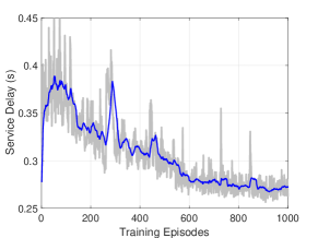
(a) Average delay performance

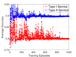
(b) Accuracy Performance of two services

Fig. 3: Performance of the proposed algorithm in the training stage.

Two types of DNN inference services are considered. Type I service: a facility fault diagnosis service to identify the fault type based on the collected bearing vibration signal from the dataset [8]. Since the duration of a time slot in the simulation is set to be one second, the task data size is the data volume of a one-second signal, which is a product of the raw sampling rate and the quantization bits of the signal. In the dataset, the bearing vibration signal is collected at 48 KHz sampling rate and 16 bit quantization, and hence the corresponding task data size is 768 kilobits. The long-term accuracy requirement of the service is set to 0.8. Type II service: a service extended from the Type I service to diagnose facility fault based on a low-grade bearing vibration dataset while requiring higher inference accuracy 0.9. The low-grade dataset collects vibration signal at a lower sampling rate of 32 KHz, and hence the task data size is 512 kilobits. For both services, the task arrival rate of each industrial IoT device at each time slot follows a uniform distribution $\mathcal{U}(\lambda-0.5,\lambda+0.5)$, where $\lambda$ is the average task arrival rate. We consider four candidate sampling rates for industrial IoT devices, which are 25%, 50%, 75% and 100% of the raw sampling rate. The corresponding accuracy with respect to the sampling rates are 0.59, 0.884, 0.950 and 0.987, respectively, based on extensive experiments on the bearing vibration dataset [8]. Balance parameter $V$ is set to 0.05 based on extensive simulations. Other important simulation parameters are listed in Table II. The parameters of the proposed algorithm are given in Table III. The proposed algorithm is compared to the following benchmarks:

• Delay myopic: Each industrial IoT device dynamically makes sampling rate selection and task offloading decisions by maximizing the one-step reward in (20) according to the network state.

• Static configuration: Each industrial IoT device takes a static configuration on the sampling rate selection and task offloading decisions, which can guarantee services’ accuracy requirements.

V-B Performance Evaluation

V-B1 Convergence of the proposed algorithm

The service delay performance in the training stage is shown in Fig. 3(a). We can clearly see that the average service delay gradually decreases as the increase of training episodes, which validates the convergence of the proposed algorithm. In addition, Fig. 3(b) shows the accuracy performance for both services with respect to training episodes. The accuracy performance is not good at the beginning of the training stage, but after 1,000 episodes of training, the accuracy performance converges to the pre-determined requirements.

V-B2 Impact of task arrival rate

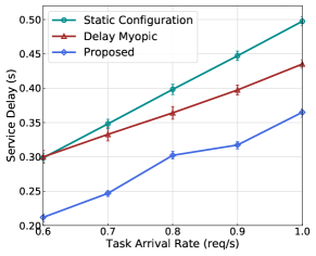
Fig. 4: Service delay performance with respect to task arrival rates.

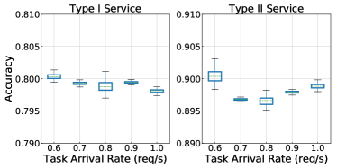
Fig. 5: Inference accuracy performance with respect to task arrival rates.

Once well-trained offline, we evaluate the performance of the proposed algorithm in the online inference. As shown in Fig. 4, we compare the average service delay performance of the proposed algorithm with benchmark schemes in terms of task arrival rates for $W=20$ MHz. Each simulation point is plotted with a 95% confidence interval. Several observations can be obtained from the figure. Firstly, the service delay increases with the task arrival rate due to constrained communication and computing resources in the network. Secondly, the proposed algorithm significantly outperforms benchmark schemes. The reason is that the proposed RL-based algorithm can capture network dynamics, such as the task arrival pattern and channel condition variation, via interacting with the environment. The learned knowledge is utilized to make online decisions that target at the long-term performance, while benchmark schemes only focus on the short-term performance and do not adapt to network dynamics. Specifically, the proposed algorithm can reduce the average service delay by 19% and 25%, respectively, as compared with delay myopic and static configuration schemes.

As shown in Fig. 5, boxplot accuracy distribution of two services is presented with respect to different task arrival rates. The long-term accuracy requirements for two services are 0.8 and 0.9, respectively. It can be seen that the proposed algorithm guarantees the long-term accuracy requirements of both services with a high probability. Specifically, the maximum error probability is less than 0.5%.

V-B3 Impact of communication bandwidth

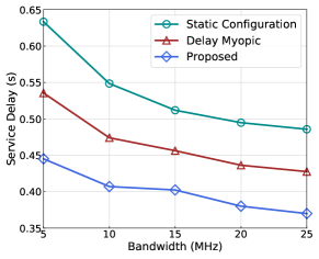
Fig. 6: Service delay performance with respect to communication bandwidth.

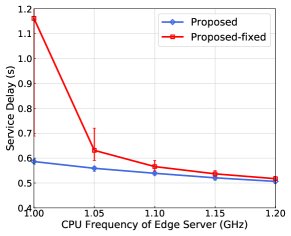
Fig. 7: Service delay in terms of CPU frequency of the edge server.

Fig. 6 shows the impact of communication bandwidth on the average service delay. Firstly, we can see that the average service delay decreases as the growth of bandwidth. The reason is that the transmission delay is reduced when the communication resource becomes sufficient. In addition, the proposed algorithm achieves good performance when the bandwidth is scarce. When system bandwidth is only 5 MHz, the proposed algorithm achieves 1.20$\times$ and 1.42$\times$ delay reduction compared with delay myopic and static configuration schemes, respectively, which is larger than that when the system bandwidth is 25 MHz (1.15$\times$ and 1.31$\times$). The reason is that the proposed algorithm efficiently utilizes the on-board computing resources. Simulation results show that the proposed algorithm decides 47.5% computation tasks to be executed locally with 5 MHz bandwidth, while the delay myopic benchmark only decides 17%. Due to the efficient resource orchestration among industrial IoT devices and the AP, the proposed algorithm can effectively reduce average service delay for both services.

V-B4 Impact of optimization subroutine

As shown in Fig. 7, we evaluate the performance of the proposed algorithm with the fixed computing resource allocation (referred to as proposed-fixed), in which the edge computing resource is allocated based on the average computing demand of two services. Compared with the proposed-fixed solution, the proposed algorithm achieves significant performance gain when the edge computing resource is constrained. Specifically, the performance gain in reducing the service delay decreases from 1.98$\times$ at 1 GHz CPU frequency to only 1.02$\times$ at 1.2 GHz CPU frequency. The reason is that efficient resource allocation is more important in resource-constrained scenarios, as compared to resource-rich scenarios. The results validate the effectiveness of the optimization subroutine for edge computing resource allocation. In addition to the performance gain, another merit of the optimization subroutine is to reduce the training complexity of RL algorithms.

VI Conclusion

In this paper, we have studied the sampling rate adaption and resource allocation problem for collaborative DNN inference in industrial IoT networks. A deep RL-based algorithm has been developed to determine the channel variation and the task arrival pattern which are then exploited to provide accuracy-guaranteed DNN inference services. The proposed algorithm can optimize service delay performance on the fly, without requiring statistic information of network dynamics. The Lyapunov-based transformation technique can be applied to other CMDPs. For the future work, we will investigate the impact of device mobility on the inference performance.

-A Proof of Theorem 1

Firstly, the problem is proved to be a convex optimization problem. For brevity of notations, we omit $t$ in the proof. With the definition of $\Lambda_{m}$ in (26), the objective function can be rewritten as $\sum_{m\in\mathcal{M}}{\Lambda_{m}}/{\left(c_{m}f_{b}\right)}$. The second-order derivative of the objective function shows $2\Lambda_{m}/\left(f_{b}c_{m}^{3}\right)>0$. In addition, the inequality constraint is linear. Hence, the problem is a convex optimization problem.

Secondly, a Lagrange function for the problem without considering the inequality constraints is constructed, i.e.,

$$\mathcal{L}\left(\mathbf{c},{a}\right)=\sum_{m\in\mathcal{M}}\frac{\Lambda_{m}}{c_{m}f_{b}}+a\left(\sum_{m\in\mathcal{M}}c_{m}-1\right),$$ (31)

where $a$ denotes the Lagrange multiplier. Based on Karush-Kuhn-Tucker conditions [26], we have

$$\begin{split}\frac{\partial L\left(\mathbf{c},{a}\right)}{\partial c_{m}}=-\frac{\Lambda_{m}}{f_{b}c_{m}^{2}}+a=0,\forall m\in\mathcal{M}.\end{split}$$ (32)

By solving the above equation, we can obtain $c_{m}^{\star}=\sqrt{{\Lambda_{m}}/{af_{b}}},\forall m\in\mathcal{M}.$ Substituting the above result into the complementary slackness condition $\sum_{m\in\mathcal{M}}c_{m}^{\star}-1=0$, the optimal value of $a$ is given by $a^{\star}={\left(\sum_{m\in\mathcal{M}}\sqrt{\Lambda_{m}}\right)^{2}}/{f_{b}}$. From the above equation, $a^{\star}$ takes a positive value, and hence $\{c_{m}^{\star}\}_{m\in\mathcal{M}}$ are positive values, which means constraint (23b), i.e., $c_{m}^{t}\geq 0,\forall m\in\mathcal{M}$, is automatically satisfied. Substituting $a^{\star}$ into the complementary slackness condition proves Theorem 1.

References

- [1] H. Hu, B. Tang, X. Gong, W. Wei, and H. Wang, “Intelligent fault diagnosis of the high-speed train with big data based on deep neural networks,” IEEE Trans. Ind. Informat., vol. 13, no. 4, pp. 2106–2116, Apr. 2017.
- [2] G. Gobieski, B. Lucia, and N. Beckmann, “Intelligence beyond the edge: Inference on intermittent embedded systems,” in Proc. ASPLOS, 2019, pp. 199–213.
- [3] Y. Chen, T. Krishna, J. S. Emer, and V. Sze, “Eyeriss: An energy-efficient reconfigurable accelerator for deep convolutional neural networks,” IEEE J. Solid-State Circuits, vol. 52, no. 1, pp. 127–138, Jan. 2017.
- [4] D. A. Chekired, L. Khoukhi, and H. T. Mouftah, “Industrial IoT data scheduling based on hierarchical fog computing: A key for enabling smart factory,” IEEE Trans. Ind. Informat., vol. 14, no. 10, pp. 4590–4602, Oct. 2018.
- [5] E. Li, L. Zeng, Z. Zhou, and X. Chen, “Edge AI: On-demand accelerating deep neural network inference via edge computing,” IEEE Trans. Wireless Commun., vol. 19, no. 1, pp. 447–457, Jan. 2020.
- [6] S. Han, H. Mao, and W. J. Dally, “Deep compression: Compressing deep neural networks with pruning, trained quantization and huffman coding,” arXiv preprint arXiv:1510.00149, 2015.
- [7] S. Teerapittayanon, B. McDanel, and H. Kung, “Branchynet: Fast inference via early exiting from deep neural networks,” in Proc. IEEE ICPR, 2016, pp. 2464–2469.
- [8] International Data Corporation, “Case western reserve university,” [Online]. Available: https://csegroups.case.edu/bearingdatacenter/pages/download-data-file.
- [9] G. Chen, W. Choi, X. Yu, T. Han, and M. Chandraker, “Learning efficient object detection models with knowledge distillation,” in Proc. NIPS, 2017, pp. 742–751.
- [10] P. Yang, F. Lyu, W. Wu, N. Zhang, L. Yu, and X. Shen, “Edge coordinated query configuration for low-latency and accurate video analytics,” IEEE Trans. Ind. Informat., vol. 16, no. 7, pp. 4855–4864, Jul. 2020.
- [11] S. Wang, Y. Guo, N. Zhang, P. Yang, A. Zhou, and X. Shen, “Delay-aware microservice coordination in mobile edge computing: A reinforcement learning approach,” IEEE Trans. Mobile Comput., DOI: 10.1109/TMC.2019.2957804, 2019.
- [12] X. Shen, J. Gao, W. Wu, K. Lyu, M. Li, W. Zhuang, X. Li, and J. Rao, “AI-assisted network-slicing based next-generation wireless networks,” IEEE Open J. Veh. Technol., vol. 1, no. 1, pp. 45–66, Jan. 2020.
- [13] P. Yang, N. Zhang, S. Zhang, L. Yu, J. Zhang, and X. Shen, “Content popularity prediction towards location-aware mobile edge caching,” IEEE Trans. Multimedia, vol. 21, no. 4, pp. 915–929, Apr. 2019.
- [14] K. Wang, Y. Zhou, Z. Liu, Z. Shao, X. Luo, and Y. Yang, “Online task scheduling and resource allocation for intelligent NOMA-based industrial Internet of things,” IEEE J. Sel. Areas Commun., vol. 38, no. 5, pp. 803–815, May 2020.
- [15] E. Altman, Constrained Markov decision processes. CRC Press, 1999, vol. 7.
- [16] Q. Liang, F. Que, and E. Modiano, “Accelerated primal-dual policy optimization for safe reinforcement learning,” arXiv preprint arXiv:1802.06480, 2018.
- [17] L. Lei, Y. Kuang, X. Shen, K. Yang, J. Qiao, and Z. Zhong, “Optimal reliability in energy harvesting industrial wireless sensor networks,” IEEE Trans. Wireless Commun., vol. 15, no. 8, pp. 5399–5413, Aug. 2016.
- [18] D. Bernstein, “Containers and cloud: From lxc to docker to kubernetes,” IEEE Cloud Computing, vol. 1, no. 3, pp. 81–84, Sep. 2014.
- [19] A. Krizhevsky, I. Sutskever, and G. E. Hinton, “Imagenet classification with deep convolutional neural networks,” in Proc. NIPS, 2012, pp. 1097–1105.
- [20] M. J. Neely, “Stochastic network optimization with application to communication and queueing systems,” Synthesis Lectures on Communication Networks, vol. 3, no. 1, pp. 1–211, 2010.
- [21] J. Luo, F. Yu, Q. Chen, and L. Tang, “Adaptive video streaming with edge caching and video transcoding over software-defined mobile networks: A deep reinforcement learning approach,” IEEE Trans. Wireless Commun., vol. 19, no. 3, pp. 1577–1592, Mar. 2020.
- [22] J. Xu, L. Chen, and P. Zhou, “Joint service caching and task offloading for mobile edge computing in dense networks,” in Proc. IEEE INFOCOM, 2018, pp. 207–215.
- [23] T. P. Lillicrap, J. J. Hunt, A. Pritzel, N. Heess, T. Erez, Y. Tassa, D. Silver, and D. Wierstra, “Continuous control with deep reinforcement learning,” in Proc. ICLR, 2016.
- [24] V. Petrov, A. Samuylov, V. Begishev, D. Moltchanov, S. Andreev, K. Samouylov, and Y. Koucheryavy, “Vehicle-based relay assistance for opportunistic crowdsensing over narrowband IoT (NB-IoT),” IEEE Internet of Things J., vol. 5, no. 5, pp. 3710–3723, Oct. 2018.
- [25] W. Wu, N. Cheng, N. Zhang, P. Yang, W. Zhuang, and X. Shen, “Fast mmwave beam alignment via correlated bandit learning,” IEEE Trans. Wireless Commun., vol. 18, no. 12, pp. 5894–5908, Dec. 2019.
- [26] S. Boyd, S. P. Boyd, and L. Vandenberghe, Convex optimization. Cambridge university press, 2004.