ACEs in spaces: Autocatalytic Chemical Ecosystems in Spatial Settings

Abstract

Autocatalysis is thought to have played an important role in the earliest stages of the origin of life. An autocatalytic cycle’s (AC) constituent chemicals can collectively catalyze their own recreation. When the reactions of multiple, interacting ACs are active in a region of space, they form an autocatalytic chemical ecosystem (ACE). Previous work demonstrated that, in chemostats, interactions between ACs in ACEs can be framed as analogous to those between species in biological ecosystems. Here, we extend this framework to investigate the effects of surface adsorption, desorption, and diffusion on ACE ecology. Simulating ACEs as particle-based stochastic reaction-diffusion systems in spatial settings, including open, two-dimensional reaction-diffusion systems and adsorptive mineral surfaces, we demonstrate that spatial structure can support more coexisting ACs and expose new AC traits to selection.

David A. Baum (dbaum and wisc.edu)

Introduction

In models of prebiotic chemical evolution, spatial structure is frequently invoked to facilitate the accumulation of complexity. Late in life’s origins, spatial structure would have been endogenous, with autocatalytic metabolisms constructing their own encapsulating membranes. However, life’s earliest progenitors likely lacked endogenous membranes to separate their incipient biochemistry from external environments. Spatial structure for the first life-like systems may have been supplied by external settings such as porous rocks or adsorbing mineral surfaces. Here, we focus on the continuous two-dimensional settings of mineral surfaces, which have been the focus of several origin of life theories, most notably Wächtershäuser’s surface metabolism model (1). Mineral-water interfaces would have been ubiquitous in the prebiotic environment and could have played a concentrating role for life-like chemistry, constraining diffusion, catalyzing reactions, and protecting chemicals from hydrolysis and thermal degradation (1, 2, 3, 4). Life’s oldest ancestral chemistry also may have lacked replicating genetic polymers. Nevertheless, to take part in life’s pre-cellular phylogeny, there must at least have been a capacity for self-propagation. In chemical terms, self-propagation requires the existence of at least one autocatalytic cycle (AC): a cyclic reaction pathway that results in a stoichiometric increase of a set of chemicals with each turn of the cycle (5). We call a chemical reaction network (CRN) containing multiple interacting ACs an autocatalytic chemical ecosystem (ACE). The parallel to ecosystem ecology follows because, like biological species, ACs can exhibit logistic growth when suitable food fluxes through the ecosystem (6). Moreover, as in the ecological case, pairs of ACs can interact like pairs of biological species, showing similar competitive, predator-prey, and mutualistic interactions (7). Moreover, ACEs can undergo ecological succession when the transient introduction of new chemical “seeds” activates new trophic levels composed of ACs that use existing ACs to self-propagate (8). In biological ecosystems, incorporating spatial structure is often necessary for accurate predictions of their dynamics. Well-mixed and spatially structured models of ecosystems concur in their predictions when only a single attractor state exists, but not necessarily when the system is multi-stable (9). For example, when there are two stable equilibria in an ecological model of mutually inhibiting populations, the ecological outcome is fully determined by average initial conditions in mean field models, but in spatial models the outcome can vary among simulations with the same average initial conditions (9). Extrapolating from ecosystem ecology, well-mixed models like chemostats are appropriate for ACEs with just one attractor state. For these simple ACEs, adding spatial structure to a well-mixed model should not affect the space of ecological possibilities realizable by the underlying CRN. But for more complex, multi-stable ACEs, which are of greater relevance to life’s origins, well-mixed models no longer suffice. As a context to explore the role of spatial structure, we use simple models of ACEs consisting of pairs of mutually inhibiting ACs, designed to exhibit bistability. We then show that spatial structure can support the coexistence of otherwise incompatible ACs, potentially increasing an ACE’s diversity and productive capacities. Moreover, we show that spatially heterogenous environments can select among competing ACs on the basis of spatially relevant traits like diffusivity to which selection is blind in the well-mixed case. These spatial, stochastic models illustrate the potential for adaptive change in simple CRNs that lack genetic information encoding. This may have been important to nascent life’s emergence and early accumulation of complexity.

Methodology

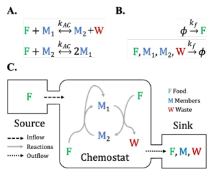
Figure 1: An autocatalytic cycle in a chemostat. (A) Reversible reactions for an AC with one food chemical ($F$), two member chemicals ($M_{1}$, $M_{2}$), and one waste chemical ($W$). We treat cycle reactions as reversible with the same rate constant $k_{AC}$ in each direction. (B) Inflow from a food source and indiscriminate outflow to a sink occur with flow rate constant $k_{f}$. We represent sources and sinks with the empty set $\phi$. (C) In a chemostat, a flux of food drives the AC reactions in the active direction, indicated by the arrowheads.

ACs & ACEs

Here, we adopt a stoichiometric definition of autocatalysis (5) that is compatible with reversible chemical kinetics (7). We categorize an AC’s chemicals as members, food, and waste. Member chemicals appear as both reactants and products across the set of AC reactions. Food and waste are categorized relative to the reaction direction that results in a stoichiometric increase in member chemicals, deemed the ACs active direction. Food chemicals only appear as reactants in the active direction, whereas waste chemicals only appear as products (Fig. 1A). When all of the ACs reactions can proceed in the active direction, we deem the AC active. When an adequate supply of food and removal of waste drives an AC’s reactions in the active direction, for example in a chemostat (Fig. 1B-C), the AC self-propagates. An active AC’s ability to self-propagate is independent of the types of chemicals involved, which can range from small molecules to long polymers to multi-molecular assemblies.

Discreteness & Stochasticity

Prior studies simulated ACE dynamics in chemostats using mass-action kinetics. Here, we opt instead for stochastic methods that track discrete chemical counts. Stochastic methods capture the environmental and demographic stochasticity characteristic of real biological ecosystems. Likewise, they are more relevant to origins of life scenarios where rare reactions and small numbers of chemicals could have played significant roles (10, 11). With stochasticity, an active AC can deactivate when the last of its member chemicals is lost (Fig. 2A). This contrasts with mass action models where the chemical concentrations of member chemicals never drop to zero but, instead approach it asymptotically. Likewise, a single dispersed seed molecule can stochastically colonize a new location by activating an AC there (Fig. 3B). The most common stochastic method for simulating chemical reaction networks is Gillespie’s exact Stochastic Simulation Algorithm (SSA) (12). The SSA treats chemistry as a continuous-time Markov process in which chemicals participate in stochastic inflow, outflow, and reaction events. In a chemostat, the SSA tracks propensities of reactions and outflow events, as calculated from dynamic chemical counts and fixed rate constants. The propensities of inflow reactions assume a fixed source food count. The amount of food flowing in from the source affects the AC’s carrying capacity. When that carrying capacity is small, the effects of stochasticity become more apparent (Fig. 2). In simulations of a simple AC in a chemostat (Fig. 1C), the SSA’s discrete count trajectories (Fig. 2A-C) converge to an ODE’s continuous concentration curves (Fig. 2D) as the AC’s carrying capacity grows.

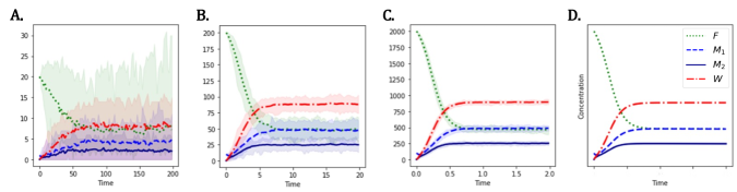
Figure 2: Discrete stochastic simulations converge to continuous deterministic simulations. (A-C) Lines indicate mean values of chemical counts over 10 replicate SSA simulations for food ($F$), member species ($M_{1}$, $M_{2}$), and waste ($W$). Shaded regions show the range of values observed. We set the source food count to 20 $F$ (A), 200 $F$ (B), and 2000 $F$ (C). Reactors were initialized with the source food count and a seed of $M_{1}$ molecules proportional to the food: 1 $M_{1}$ (A), 10 $M_{1}$ (B), and 100 $M_{1}$ (C). (D) Simulation with mass action kinetics and a source food concentration of 200 units $F$, and a seed set to 10 units $M_{1}$ to maintain the same source-to-seed ratio as the SSA simulations. Concentration units are arbitrary. Each simulation was run with $k_{AC}=k_{f}=0.01$.

Spatial Structure

Next, we add spatial structure by modelling an ACE as a particle-based stochastic reaction-diffusion system, where stochastic reactions occur locally in a hexagonal lattice of discrete sites and stochastic diffusion transfers chemicals between sites. The combination of discreteness, stochasticity, and spatial structure in a particle-based stochastic reaction-diffusion system allow for richer and more realistic ecological dynamics. Their explicit spatial structure, which spatially localizes sites and connects neighbors, contrasts with patch models, and their discretness and stochasticity contrasts with deterministic reaction-diffusion models, resulting in qualitative behavior that these other modeling approaches fail to capture (9). For example, the presence of multiple stable states has been shown to support coexistence of competitors in models that are discrete, stochastic, and spatial, even when they could not coexist in models that lack one or more of these attributes (13). Each site in the hexagonal array is treated as a chemostat and simulated with the SSA. Stochastic diffusion events moving particles (chemicals) between adjacent sites occur in addition to inflow, outflow, and reaction events within each site (Fig. 3A). All chemicals diffuse stochastically according to their counts at each site and diffusion rate constants (14). To validate the model, we showed that an AC seeded at one location can expand radially as its member species stochastically colonize adjacent sites (Fig. 3B). For simulations with larger chemical reaction networks or larger spatial settings, we employ τ-leaping, an efficient approximation of the SSA that updates reaction propensities less frequently (15, 16).

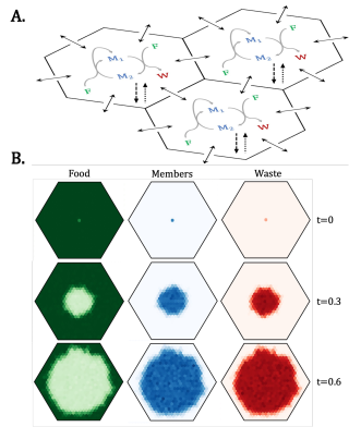
Figure 3: Growth and diffusion in a 2D setting. (A) A section of a hexagonal reaction-diffusion array. In each site, food flows in from a source (dashed arrows), all chemicals flow out to a sink (dotted arrows), react (gray arrows), and diffuse to adjacent sites (solid black arrows). (B) An AC seeded in the center of a hexagonal reaction-diffusion array of diameter 31 with periodic boundaries. Heatmaps show the counts of food (left, green), total member chemicals (middle, blue), and waste (right, red) at three time points. Each site was initialized with the source food count of $1000F$ and the central site contains a seed of $250M_{1}$. The simulation was run for a total time $T=6.7$ with $k_{AC}=k_{f}=0.01$, diffusion rate constant $k_{D}=0.6$, and $\tau$-leaping.

Bistable ACEs

We designed several ACEs, each consisting of a pair of mutually inhibiting ACs, A and B. Any ACE with a viable AC is trivially multi-stable because that AC could be active or inactive. Here, we use bistability to refer to cases in which each AC could remain active on its own, but cannot coexist with the other in a well mixed setting, providing just two stable ecological outcomes if both ACs are initially active: either A will deactivate B, or B will deactivate A. Our first mechanism for mutual inhibition (Fig. 4A-C) was previously explored in (7) for its ability to demonstrate dynamics resembling ecological succession. For this mechanism, we use two-member ACs (the simplest ACs that generate waste while retaining second order reactions) that do not share food or waste. Mutual inhibition arises because each AC’s waste reacts with two of the other AC’s food to produce another chemical (not explicitly modeled) that neither AC can directly use. As one AC grows, its accumulating waste saps the other’s food, thereby deactivating its reactions. Making the inhibition reactions reversible only slightly raises the inhibition rate constant, $k_{I}$, required to achieve bistability, so we simplify the system by modelling the inhibition through (irreversible) annihilation reactions. Our second mechanism for mutual inhibition (Fig. 4D-F) uses two single-member ACs whose member chemicals react irreversibly to form another chemical (again not explicitly modeled). As in the first case, making this inhibition reaction reversible only slightly lowers the numerical threshold for bistability, so we model it as an annihilation reaction for simplicity. Reactions between any two member chemicals of ACs with multiple members can be sufficient for bistability, but because food and waste are not involved in this inhibition mechanism, we simplify the system by modelling single-member ACs with no waste. Additionally, because simple competition for food is not sufficient for bistability in ACEs with reversible reactions (Peng et al., 2020), we further simplify the system by having these ACs share food. This mechanism for bistability contains the fewest number of reactions, making its simulations the least computationally demanding of the CRNs studied. Our third mechanism for inhibition models the catalytic role that mineral surfaces are thought to have played in prebiotic chemistry. We separate the reaction diffusion system into a diffusive layer subject to inflow, outflow, and diffusion and a surface layer where AC reactions take place, but not diffusion (Fig. 4I). The member chemicals of each AC adsorb and desorb between the diffusive and surface layers (Fig. 4G-H). Whereas the diffusive layer is treated as having an unlimited capacity for chemicals, a finite number of adsorption sites are defined at each location in the surface layer. Mutual inhibition arises because of zero-sum competition for these surface sites. Each AC’s self-propagation requires that a member chemical be adsorbed and that an additional open adsorption site be available for the new member chemical produced. An AC that occupies open adsorption sites can, therefore, inhibit the self-propagation of the other AC. We neglect reactions in the diffusive layer, which amounts to the assumption that surface catalyzed reactions occur at much faster rates. Additionally, we treat the active direction of each AC’s reactions as thermodynamically favored and simplify the system by only modeling the active direction.

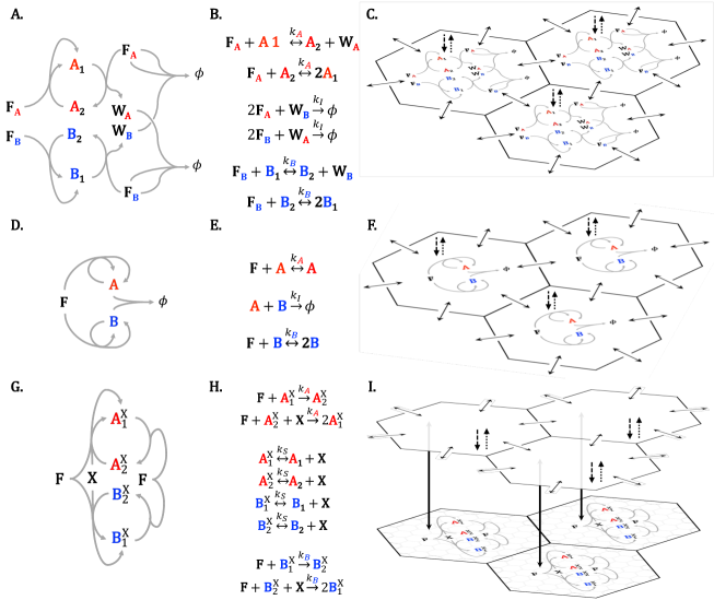
Figure 4: ACE with bistability via waste-food reactions. ACEs exhibiting bistability via waste food reactions. (A-C), member chemical reactions (D-F), and surface competition (G-I). (A, D, G) CRNs. Arrows indicate inhibition reactions and the active direction of AC reactions. (B, E, H) Chemical reactions and their rate constants (in addition to food inflow and indiscriminate outflow). (C, F) Sections of hexagonal reaction-diffusion array. In each site, food flows in from a source (dashed arrows), all chemicals flow out to a sink (dotted arrows), react (gray arrows), and diffuse to adjacent sites (solid black arrows). (I) A two-layer reaction-diffusion system consisting of a diffusive layer with diffusion, inflow, and outflow, and a surface layer with surface-catalyzed AC reactions.

Metrics

To quantify the differences between ecological outcomes in spatial settings, we use several descriptive metrics. We track the sum of each AC’s members at each site $i$ as $A_{i}$ and $B_{i}$. The local relative frequencies of members are defined as $P_{A,i}=\frac{A_{i}}{A_{i}+B_{i}}$ and $P_{B,i}=\frac{B_{i}}{A_{i}+B_{i}}$ respectively and local occupancy ($O_{i}$) is the difference between these frequencies: $O_{i}=P_{A,i}-P_{B,i}$. Similarly, the global relative frequencies, $P_{A}=\frac{A}{A+B}$ and $P_{B}=\frac{B}{A+B}$, are obtained from total counts of each AC’s members over all N sites: $A=\sum_{i=1}^{N}A_{i}$ and $B=\sum_{i=1}^{N}B_{i}$, and global relative occupancy ($O$) is $O=P_{A}-P_{B}$. Occupancy values ranges from -1 (full occupation by $B$) to 1 (full occupation by $A$). We also define three measures of heterogeneity. First, to capture the degree of correlation between neighboring sites, we define neighborhood heterogeneity ($H_{nei}$):

$${H_{nei,i}=\frac{1}{12}\sum_{j=1}^{6}|O_{i}-O_{j}|,}$$ (1)

where $j$ ranges over the six nearest neighbors of site $i$. Second, to capture the variation within each site, we define local heterogeneity ($H_{loc}$) as an entropy of the local relative frequencies of each AC’s member chemicals:

$${H_{loc,i}=-P_{A,i}\log_{2}{P_{A,i}}+P_{B,i}\log_{2}{P_{B,i}}.}$$ (2)

Aggregate neighborhood and local heterogeneity is $H_{nei}=\frac{1}{N}\sum_{i=1}^{N}H_{nei,i}$ and $H_{loc}=\frac{1}{N}\sum_{i=1}^{N}H_{loc,i}$. Third, we define global heterogeneity ($H_{glob}$) as the entropy of the global relative frequencies:

$${H_{glob}=P_{A}\log_{2}{P_{A}}+P_{B}\log_{2}{P_{B}}.}$$ (3)

All three heterogeneity measures range between 0 (low heterogeneity) and 1 (high heterogeneity). In ecological terms, $H_{loc}$ is alpha diversity and $H_{glob}$ is gamma diversity (17).

Results

The Effect of Diffusion on Coexistence in a Bistable ACE

First, we explore the effect of chemical diffusivities on ACE dynamics. To simulate a larger reaction-diffusion system where patterns are more apparent and larger statistical samples can be taken, we use the simplest bistability mechanism (Fig. 4D-F). We simulate a hexagonal reaction-diffusion system of diameter 38 with periodic boundaries, seeded uniformly with equal quantities of A and B, and vary the diffusion rate constant $k_{D}$ of member chemicals. To highlight the effects of diffusion, we set all reaction rate constants equal. And because food is continuously resupplied and consumed by each AC with equal rate constants, we neglect the diffusion of food chemicals. To illustrate the effects of diffusion, Fig. 5 shows the spatial distribution of $O_{i}$,$H_{loc,i}$, and $H_{nei,i}$ at the final time step for six diffusion rates. Fig. 6 shows $H_{loc}$, $H_{nei}$, and $H_{glob}$ for 50 diffusion values through time (Fig. 6).

The slow diffusion regime reaches low $H_{loc}$ and high $H_{glob}$ because the ACs do not coexist locally but remain active in nearly equal quantities globally. In contrast, the high diffusion regime converges towards low $H_{loc}$ and low $H_{glob}$ because one AC drives the other extinct everywhere, though it does so slowly such that $H_{loc}$ remains transiently high. The intermediate diffusion regime attains intermediate values of both $H_{glob}$ and $H_{loc}$. Notably, $H_{loc}$ peaks where there is intermediate diffusion.

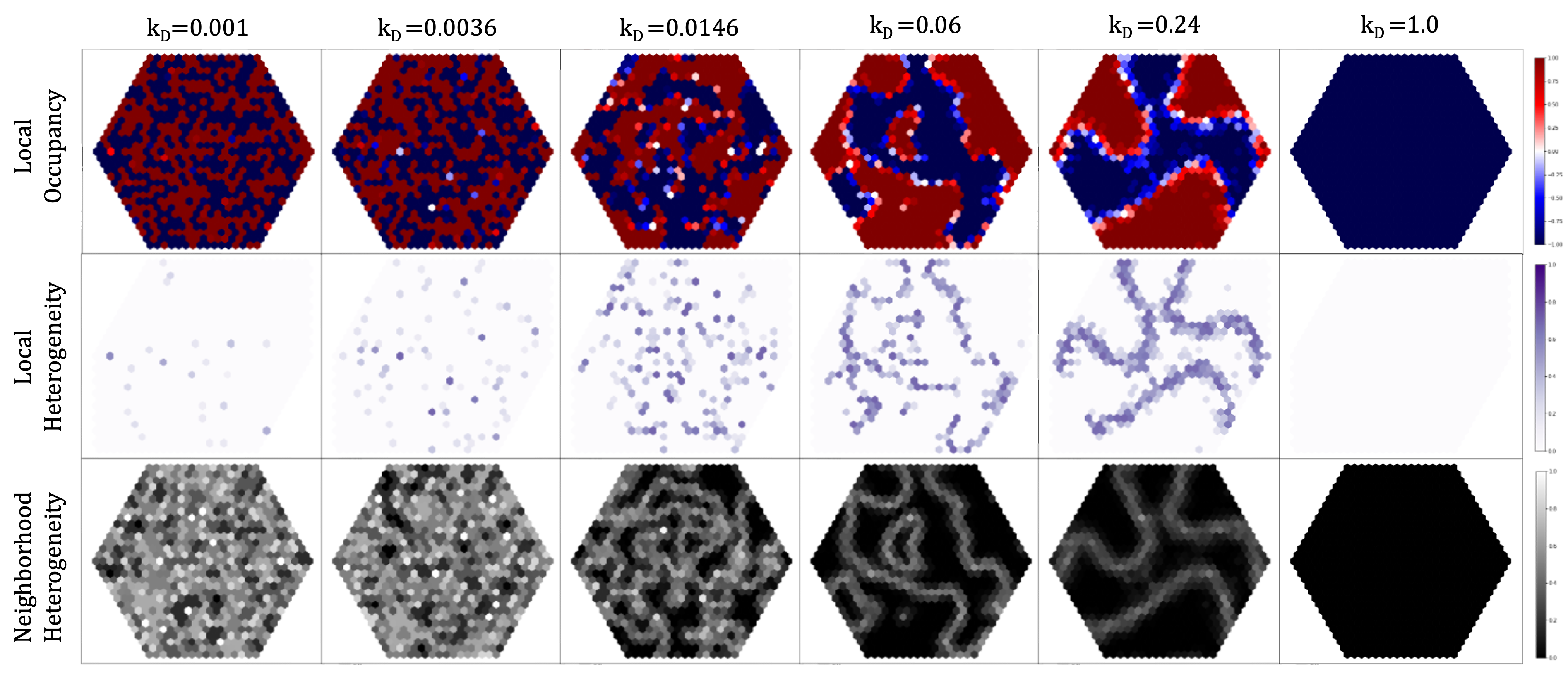
Figure 5: Snapshots of the final state of each ACE. Heatmaps of $O_{i},H_{loc,i},$ and $H_{nei,i}$ at locations in a hexagonal reaction-diffusion array of diameter 39 for member chemical diffusivity values $k_{D}$ ranging logarithmically from $10^{-3}$ to 1. Each site was seeded with 10 $A$, 10 $B$, and 50 $F$. Each simulation was run to time $T=100$ with $k_{AC,A}=k_{AC,B}=0.01$,$k_{f}=0.01$, $k_{I}=0.02$, source food count 50 $F$, and $\tau$-leaping.

With low diffusion, one AC quickly occupies and deactivates the other AC in each site. Because so few chemicals are exchanged between sites, neither AC can successfully invade a site occupied by the other, so each site quickly converges to a steady state with low $H_{loc}$. However, because sites can become stably occupied by either AC, $H_{glob}$ remains high. With high diffusion, adjacent sites exchange large numbers of chemicals and exhibit spatially autocorrelated dynamics. In the extreme case, the dynamics approximate a single well-mixed chemostat, resulting in global bistability with $H_{glob}$ dropping to 0. In intermediate diffusion regimes, however, sites may transition between periods of occupation by each AC as they successfully invade one another’s sites. This results in patches of the surface occupied by each AC. The patch size increases with $k_{D}$ (Fig. 5), reminiscent of the temperature dependent correlation length of the 2D Ising model (18). In both the low and intermediate diffusion regimes, the ACE exhibits long-term coexistence of its mutually inhibiting ACs, but the intermediate regime entails ongoing interaction between the ACs’ chemicals resulting in a greater chemical diversity near the boundaries between patches.

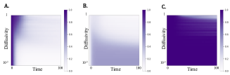
Figure 6: Measures of Heterogeneity. Heatmaps of (A) $H_{loc}$, (B) $H_{nei}$, and (C) $H_{glob}$ through time for simulations with member chemical diffusivities ranging logarithmically from $10^{-3}$ to 1. Heatmap values average over 10 replicate simulations. Each simulation was run for a total time T = 100 with $k_{AC,A}=k_{AC,B}=0.01,k_{f}=0.01,k_{I}=0.02$, source food count 50 $F$, and $\tau$-leaping.

Diffusivity as a selective advantage among mutually inhibiting ACs

Next, we investigate the role of member chemical diffusivity in the ecological interactions of mutually inhibiting ACs. Whereas before each AC had the same reaction and diffusion rate constants, here we vary them separately. We say that an AC is fiercer if its reaction rate constants are higher. We say that an AC is faster if its member chemicals have higher diffusivity. To assess the comparative advantages of each, we explore the effects of makinf $A$ fiercer than $B$ and of making $B$ faster than $A$. Thus, $A$ tends to self-propagate more rapidly using available food whereas $B$ tends to reach new sites faster to exploit new sources of food. For these computational experiments, we use waste-food reactions as the mechanism for mutual inhibition (Fig. 4A-C). We simulate these ACs in hexagonal reaction-diffusion system of diameter 7 with periodic boundaries, varying the fierceness advantage of $A$ and the fastness advantage of $B$. For each parameter combination, we seed both cycles in equal quantities in the central site, initializing food uniformly. In the central site, $A$, being fiercer, begins to deactivate $B$. In some conditions, $A$ can then spread out and occupy all sites (Fig. 7A). However, because all other sites are initially unoccupied, $B$, being faster, can sometimes reach unoccupied sites fast enough to establish occupancy advantages against subsequent invasions by $A$. Further, $B$ can sometimes reinvade the central site to deactivate the fiercer AC globally (Fig. 7B). Looking across a range of values we see that $B$ can only achieve a finite occupancy advantage and that beyond some threshold of relative fierceness $A$ will always dominate. Below this threshold, an AC with faster diffusing members can outcompete one with higher reaction rate constants (Fig. 7C).

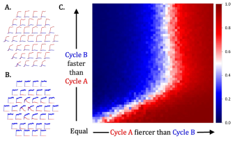
Figure 7: Fast vs. fierce with chemical inhibition. (A-B) Time series for each AC’s member chemicals at each site for sample parameter combinations. The fiercer AC (A) dominates for the parameter combination ($k_{AC,B}=0.004,k_{D,B}=10$). The faster AC (B) dominates for the parameter combination ($k_{AC,B}=0.008$, $k_{D,B}=10$). (C) Ecological phase diagram of global occupancy at the final time for different parameter combinations, averaged over 10 replicates. From left to right, $k_{AC,B}$ decreases logarithmically from $10^{-2}$ to $10^{-2.5}$. From bottom to top, the diffusion constant for B’s member chemicals, $k_{D,B}$, increases logarithmically from $10^{-1}$ to $10^{3}$. Simulations take place in a hexagonal reaction-diffusion system of diameter 7 with periodic boundaries. The central site was seeded with $10$ $A_{1}$ and $10$ $B_{1}$ and each site was seeded with $1000$ $F$. Each simulation was run to time $T=10$ with $k_{AC,A}=10^{-2}$, $k_{f}=10^{-1}$, $k_{I}=1$, $k_{D,A}=10^{-1}$, source food count $1000$ $F$, and $\tau$-leaping.

We repeat these experiments with the third mechanism for mutual inhibition: adsorption site competition (Fig. 4G-I) and obtain similar results (Fig. 8). In a chemostat, the fiercer AC will always be favored. Nonetheless, as with the first inhibition mechanism, we find that there is a parameter range in which fastness is favored over fierceness (Fig. 8C).

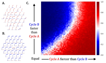
Figure 8: Fast vs. fierce with surface inhibition. (A-B) Time series of the member species of each AC at each site for sample parameter combinations. (A) A dominates for the parameter combination ($0.008$, $10$). (B) B dominates for the parameter combination ($0.004$, $10$). (C) Ecological phase diagram of the relative abundance of each AC’s member chemicals at the end of the simulation for different parameter combinations. From left to right, B’s reaction rate constants decrease from $10^{-3.5}$ to $10^{-2}$. From bottom to top, B’s diffusion rate constant increases from $10^{-1}$ to $10^{3}$. Simulations were conducted in a hexagonal reaction-diffusion of diameter 7 with periodic boundaries. Each site was seeded with $100$ $F$ and contained $100$ adsorption sites. The central site was seeded with $10A_{1}$ and $10B_{1}$. Each simulation was run with adsorption and desorption rate $k_{S}=10^{-2}$, $k_{A}=10^{-2}$, $k_{f}=10^{-1}$, $D_{A}=10^{-1}$, total time $T=30$, source food count $100F$, and $\tau$-leaping.

Discussion

Spatial structure enriches ACE dynamics

Our in-silico experiments show that spatial structure enriches the dynamics of ACEs in several ways. Most obviously, spatial structure increases global chemical diversity by eliminating convergence to a single global attractor in which some chemicals cease production. In intermediate diffusion regimes, spatial structure can also accommodate transient patches and patterns. Moreover, intermediate diffusion can contribute additional ACE diversity when it facilitates ongoing interaction between ACs who mutually inhibit one another through reactions between their food, members, or waste. This parallels the more general finding in biology that "Complex systems when combined with slight migration between them produce even more complex systems with more possibilities and representations of stable polymorphisms" (19). Reactions between AC chemicals will produce other, presumably larger, chemicals so long as the ACs continue to coexist locally. In a well-mixed setting, that diversity will vanish because one of the necessary ACs will be deactivated globally. Likewise, in sets of isolated reactors, they will vanish because one of the two ACs will be deactivated locally everywhere. It is only with intermediate diffusion that both ACs would continue to actively inhibit one another and thereby add chemical diversity to the ACE. Mineral surfaces provide one way of achieving an intermediate diffusion regime, confining the dynamics to 2D and lowering effective diffusion rates through chemical adsorption.

A second implication of spatial structure is that it adds factors that can be respond to selection. Our study varying diffusion symmetrically resembles pure genetic drift in that neither AC has an intrinsic advantage over the other yet one or the other is expected to go to fixation eventually by chance. In contrast, our study varying reaction rates and diffusion rates asymmetrically resembles selection, since ACs differentially persist and propagate on account of intrinsic differences. We demonstrated that diffusivity can be a target of selection in settings where sites are initially unoccupied, something which could not occur in well-mixed cases, where diffusion has no meaning and there is only one site to occupy. Our results suggest that with patchily distributed resources or intermittent disturbances, ACEs could come to be dominated by fast dispersing “weak” ACs, which might allow for richer chemical diversity than the fierce ACs that tend to dominate under low disturbance. This finding suggests a possible chemical analog of the intermediate disturbance hypothesis (20). Spatial structure has been shown elsewhere to create new ACs when it affects the underlying CRN (5). Blockhuis et al. provide an example of a CRN affording no ACs in a well-mixed setting that nevertheless has one AC when operating in two connected compartments that are each conducive to a different subset of reactions. As we have shown, a mineral surface can effectively create two compartments by allowing a distinction between adsorbed and desorbed chemicals, permitting catalyzed reactions in the adsorbed layer, and shielding adsorbed chemicals from direct inflow or outflow. Similarly, one can imagine additional dynamical and selective complexity emerging in other spatial settings, such as selectively permeable compartments.

ACEs in spaces blur boundaries between ecological and evolutionary concepts

Biological ecosystems, like organisms themselves, are complex adaptive systems (21) whose accumulation of complexity does not depend solely on the Darwinian evolution of the populations that compose them. Even in the absence of Darwinian evolution, ecosystem complexity can arise through self-organization (22), endogenous pattern formation (23), and autocatalytic niche emergence (24), where niche emergence drives ecological diversity and that diversity drives the emergence of new niches (25). By analogy, ACEs can accumulate complexity in a manner analogous to biological ecosystems without the evolvability of ACs themselves (7, 8).

Natural selection can act on chemical processes insofar as they have a capacity to self-propagate, change, and propagate their changes. While individual ACs can self-propagate, they lack capacity for variation. An AC might change by deactivating existing reactions and activating new reactions while remaining a closed cycle. But only so many paths can circle back to the same chemicals without forming other cycles along the way. Thus, individual ACs make weak candidate units of selection (26). The untapped creative potential of ACs lies not in their ability to evolve, but in their potential to stably organize in unprestatable combinations and contexts (27, 28), each with their own constructive and catalytic capacities. ACEs have a much greater capacity for variation because they can contain many different active ACs, with different combinations conferring different ecosystem-level properties. As a result, the set of possible, propagable changes to any ACE will usually be much larger than the "adjacent possible" (27) for any individual AC. ACEs’ increased capacity for variation makes them stronger candidate units of selection. Evolution can be seen to occur when the set of active ACs composing an ACE change through the deactivation of existing ACs or the activation of new ones (8). This resonates with the ecosystem-first theory of life’s origins (29) in which the primitive adaptive dynamics of interacting chemical processes preceded and provided for the emergence of paradigmatic Darwinian evolution at a later stage in the origin of life. When there are many separated but interconnected ACEs, ACEs could comprise a primitive Darwinian population that may be termed an autocatalytic chemical meta-ecosystem (ACME).

Though separated in space, these ecosystems can have material flow between them. In some cases, meta-ecosystem flows couple local ecosystem dynamics. For ACMEs, flows of chemicals between ACEs can complicate their adaptive dynamics just as horizontal gene transfer can complicate phylogenetic trees in biology. Thus, the degree of separation and stable boundaries that ACEs maintain has implications for their evolvability. Trivially, spatial structure is necessary for boundaries to exist between ACEs at all and as we have shown, chemical diffusivities can affect the extent and stability of those boundaries. When ACEs form patches with stable boundaries, they may behave like discrete units even without cellular encapsulation (30). Considering ACMEs simultaneously allows us to incorporate the theoretical frameworks of spatial ecosystem ecology into chemical ecosystem ecology and to conceptualize ACEs as units of selection in Darwinian populations. Here, we have focused on the former, but note implications for the latter.

Avenues for Future Work

Future work on ACEs in spatially structured settings can expand both the CRNs considered and the spatial structures within which they are simulated. Here we have confined our experiments to pairs of mutually inhibiting ACs. Within this narrow scope, other mechanisms for mutual inhibition are possible. For example, one AC’s waste can react with another AC’s members. Additionally, there are other routes to nontrivial bistability that do not involve mutual inhibition, such as the Schlögl model (31), which achieves bistability with just one AC. Drawing on theoretical ecology, predation, which has been demonstrated in ACEs (7), can exhibit complex dynamics in space (32). When more than two ACs are present, there is also the possibility of multistability via unidirectional inhibition, for example, when three ACs may inhibit one other cyclically, coexisting in an ecological game of rock, paper, scissors (33). Other ACEs of interest may emulate Turing mechanisms through short-range autocatalytic activation and long-range inhibition of ACs (34, 35).

Here, we have focused on 2D reaction-diffusion systems and mineral surfaces, assuming spatially uniform inflow and outflow. However, localized sources and sinks are also possible. Moreover, analogous to way that life makes use of both active and passive transport, ACEs may be affected by advection when there are velocity fields generated by other spatial gradients in the environment. Supplying spatial directionality to an ACME may result in different parts being functionally upstream or downstream of others, which could yield patterns resembling ecological clines. ACMEs with directional flow between ACEs could begin with simple precursors and have the byproducts of upstream ACEs supply a greater diversity of chemical inputs to downstream ACEs.

Another obvious class of models to explore would be protocell-like spatial structures, in which some chemicals are only periodically (if ever) exchanged between reactors. There are reasons to suppose that more discrete spatial structures may provide greater protection for the prebiotic chemistry they harbor (36, 37) and result in ACMEs that resemble populations of protocells, facilitating natural selection. The simplest models would assume that these discrete structures are provided by the external environment, but more sophisticated models might allow for the possibility that ACEs delimit or reinforce their own boundaries, for example by producing amphiphiles that tend to form vesicles. Such spatial models might ultimately allow us to build a plausible pathway from systems whose spatial structure is imposed externally via mineral surfaces, pores, or externally generated compartments, to ACEs that individuate themselves. Indeed, we would argue that a worthwhile long-term goal of studies of the spatial aspects of prebiotic chemical dynamics should be to explain autopoiesis (38) and the transition from exogenous to endogenous spatial structure.

This research was funded by the NASA-NSF CESPOoL (Chemical Ecosystem Selection Paradigm for the Origins of Life) Ideas Lab grant (NASA grant 80NSSC17K0296).

Bibliography

References

- Wächtershäuser (1988) Günter Wächtershäuser. Before enzymes and templates: theory of surface metabolism. Microbiological reviews, 52(4):452–484, 1988.
- Wächtershäuser (1990) Günter Wächtershäuser. Evolution of the first metabolic cycles. Proceedings of the National Academy of Sciences, 87(1):200–204, 1990.
- Wächtershäuser (1992) Günter Wächtershäuser. Groundworks for an evolutionary biochemistry: the iron-sulphur world. Progress in biophysics and molecular biology, 58(2):85–201, 1992.
- Ferris et al. (1989) James P Ferris, Gözen Ertem, and Vipin Agarwal. Mineral catalysis of the formation of dimers of 5’-amp in aqueous solution: the possible role of montmorillonite clays in the prebiotic synthesis of rna. Origins of Life and Evolution of the Biosphere, 19(2):165–178, 1989.
- Blokhuis et al. (2020) Alex Blokhuis, David Lacoste, and Philippe Nghe. Universal motifs and the diversity of autocatalytic systems. Proceedings of the National Academy of Sciences, 117(41):25230–25236, 2020.
- Lloyd (1967) PJ Lloyd. American, german and british antecedents to pearl and reed’s logistic curve. Population Studies, 21(2):99–108, 1967.
- Peng et al. (2020) Zhen Peng, Alex M Plum, Praful Gagrani, and David A Baum. An ecological framework for the analysis of prebiotic chemical reaction networks. Journal of theoretical biology, 507:110451, 2020.
- Peng et al. (2022) Zhen Peng, Jeff Linderoth, and David A Baum. The hierarchical organization of autocatalytic reaction networks and its relevance to the origin of life. PLOS Computational Biology, 18(9):e1010498, 2022.
- Durrett and Levin (1994) Richard Durrett and Simon Levin. The importance of being discrete (and spatial). Theoretical population biology, 46(3):363–394, 1994.
- Wu and Higgs (2009) Meng Wu and Paul G Higgs. Origin of self-replicating biopolymers: autocatalytic feedback can jump-start the rna world. Journal of molecular evolution, 69(5):541–554, 2009.
- Wu and Higgs (2012) Meng Wu and Paul G Higgs. The origin of life is a spatially localized stochastic transition. Biology direct, 7(1):1–15, 2012.
- Gillespie (1976) Daniel T Gillespie. A general method for numerically simulating the stochastic time evolution of coupled chemical reactions. Journal of computational physics, 22(4):403–434, 1976.
- Levin (1974) Simon A Levin. Dispersion and population interactions. The American Naturalist, 108(960):207–228, 1974.
- Erban et al. (2007) Radek Erban, Jonathan Chapman, and Philip Maini. A practical guide to stochastic simulations of reaction-diffusion processes. arXiv preprint arXiv:0704.1908, 2007.
- Anderson (2008) David F Anderson. Incorporating postleap checks in tau-leaping. The Journal of chemical physics, 128(5):054103, 2008.
- Cao et al. (2006) Yang Cao, Daniel T Gillespie, and Linda R Petzold. Efficient step size selection for the tau-leaping simulation method. The Journal of chemical physics, 124(4):044109, 2006.
- Daly et al. (2018) Aisling J Daly, Jan M Baetens, and Bernard De Baets. Ecological diversity: measuring the unmeasurable. Mathematics, 6(7):119, 2018.
- Onsager (1944) Lars Onsager. Crystal statistics. i. a two-dimensional model with an order-disorder transition. Physical Review, 65(3-4):117, 1944.
- Karlin and McGregor (1972) Samuel Karlin and James McGregor. Application of method of small parameters to multi-niche population genetic models. Theoretical Population Biology, 3(2):186–209, 1972.
- Connell (1978) Joseph H Connell. Diversity in tropical rain forests and coral reefs: high diversity of trees and corals is maintained only in a nonequilibrium state. Science, 199(4335):1302–1310, 1978.
- Levin (1998) Simon A Levin. Ecosystems and the biosphere as complex adaptive systems. Ecosystems, 1(5):431–436, 1998.
- Levin (2005) Simon A Levin. Self-organization and the emergence of complexity in ecological systems. Bioscience, 55(12):1075–1079, 2005.
- Levin and Segel (1985) Simon A Levin and Lee A Segel. Pattern generation in space and aspect. SIAM Review, 27(1):45–67, 1985.
- Cazzolla Gatti et al. (2020) Roberto Cazzolla Gatti, Roger Koppl, Brian D Fath, Stuart Kauffman, Wim Hordijk, and Robert E Ulanowicz. On the emergence of ecological and economic niches. Journal of Bioeconomics, 22(2):99–127, 2020.
- Gatti et al. (2018) Roberto Cazzolla Gatti, Brian Fath, Wim Hordijk, Stuart Kauffman, and Robert Ulanowicz. Niche emergence as an autocatalytic process in the evolution of ecosystems. Journal of theoretical biology, 454:110–117, 2018.
- Godfrey-Smith (2009) Peter Godfrey-Smith. Darwinian populations and natural selection. Oxford University Press, 2009.
- Kauffman (1996) Stuart Kauffman. Autonomous agents, self-constructing biospheres, and science. Complexity, 2(2):16–17, 1996.
- Kauffman (2000) Stuart A Kauffman. Investigations. Oxford University Press, 2000.
- Hunding et al. (2006) Axel Hunding, Francois Kepes, Doron Lancet, Abraham Minsky, Vic Norris, Derek Raine, K Sriram, and Robert Root-Bernstein. Compositional complementarity and prebiotic ecology in the origin of life. Bioessays, 28(4):399–412, 2006.
- Baum (2015) David A Baum. Selection and the origin of cells. Bioscience, 65(7):678–684, 2015.
- Schlögl (1972) Friedrich Schlögl. Chemical reaction models for non-equilibrium phase transitions. Zeitschrift für physik, 253(2):147–161, 1972.
- Murray (2001) James D Murray. Mathematical biology II: spatial models and biomedical applications, volume 3. Springer New York, 2001.
- Kerr et al. (2002) Benjamin Kerr, Margaret A Riley, Marcus W Feldman, and Brendan JM Bohannan. Local dispersal promotes biodiversity in a real-life game of rock–paper–scissors. Nature, 418(6894):171–174, 2002.
- Turing (1990) Alan Mathison Turing. The chemical basis of morphogenesis. Bulletin of mathematical biology, 52(1):153–197, 1990.
- Muñuzuri and Pérez-Mercader (2022) Alberto P Muñuzuri and Juan Pérez-Mercader. Unified representation of life’s basic properties by a 3-species stochastic cubic autocatalytic reaction-diffusion system of equations. Physics of Life Reviews, 2022.
- Shah et al. (2019) Vismay Shah, Jonathan de Bouter, Quinn Pauli, Andrew S Tupper, and Paul G Higgs. Survival of rna replicators is much easier in protocells than in surface-based, spatial systems. Life, 9(3):65, 2019.
- Takeuchi and Hogeweg (2009) Nobuto Takeuchi and Paulien Hogeweg. Multilevel selection in models of prebiotic evolution ii: a direct comparison of compartmentalization and spatial self-organization. PLoS computational biology, 5(10):e1000542, 2009.
- Luisi and Varela (1989) Pier Luigi Luisi and Francisco J Varela. Self-replicating micelles—a chemical version of a minimal autopoietic system. Origins of Life and Evolution of the Biosphere, 19(6):633–643, 1989.