Empirical Bayes When Estimation Precision Predicts Parameters

Abstract.

Empirical Bayes shrinkage methods usually maintain a prior independence assumption: The unknown parameters of interest are independent from the known precision of the estimates. This assumption is theoretically questionable and empirically rejected, and imposing it inappropriately may harm the performance of empirical Bayes methods. We instead model the conditional distribution of the parameter given the standard errors as a location-scale family, leading to a family of methods that we call close. We establish that (i) close is rate-optimal for squared error Bayes regret, (ii) squared error regret control is sufficient for an important class of economic decision problems, and (iii) close is worst-case robust. We use our method to select high-mobility Census tracts targeting a variety of economic mobility measures in the Opportunity Atlas (Chetty et al., 2020; Bergman et al., 2023). Census tracts selected by close are more mobile on average than those selected by the standard shrinkage method. For 6 out of 15 mobility measures considered, the gain of close over the standard shrinkage method is larger than the gain of the standard method over selecting Census tracts uniformly at random.

JEL codes. C10, C11, C44

Keywords. Empirical Bayes, regret, heteroskedasticity, nonparametric maximum likelihood, Opportunity Atlas, Creating Moves to Opportunity

1. Introduction

After obtaining noisy estimates for many parameters of interest, applied economists increasingly use empirical Bayes methods to shrink these estimates, in hopes to improve subsequent policy decisions. The textbook empirical Bayes method assumes prior independence—that the precisions of the noisy estimates do not predict the underlying unknown parameters. However, prior independence is theoretically questionable and empirically rejected in many contexts, and inappropriately imposing it can harm empirical Bayes decisions. Motivated by these concerns, this paper introduces empirical Bayes methods that relax prior independence.

To be concrete, our primary empirical example (Bergman et al., 2023) computes empirical Bayes posterior means for economic mobility estimates published in the Opportunity Atlas (Chetty et al., 2020). Throughout this paper, measures of economic mobility are defined as certain average outcomes of children from low-income households. Here, prior independence is the assumption that the standard errors of these noisy mobility estimates do not predict true economic mobility. However, Census tracts with more low-income households naturally have more precise estimates for outcomes of low-income children—and hence more precise estimates of economic mobility. These tracts also tend to have lower underlying economic mobility due to, for one, residential segregation (Chyn and Katz, 2021). Consequently, the standard errors of the estimates and true economic mobility are positively correlated.

Bergman et al. (2023) aim to select high mobility Census tracts by screening on empirical Bayes posterior mean estimates. Inappropriately imposing prior independence may lead to poor selections: Using a validation procedure that we develop, for several measures of economic mobility where prior independence is severely violated, we find that screening on conventional empirical Bayes posterior means selects less economically mobile tracts, on average, than screening on the unshrunk estimates. In contrast, screening on empirical Bayes posterior means computed by our method selects substantially more mobile tracts.

Section 2 introduces our method in detail. To describe our method, let $Y_{i}$ be some noisy estimates for some parameters $\theta_{i}$, with standard errors $\sigma_{i}$, over heterogeneous populations $i=1,\ldots,n$. In our empirical application, $(Y_{i},\sigma_{i})$ are published in the Opportunity Atlas for each Census tract $i$ and are designed to measure true economic mobility $\theta_{i}$. Motivated by the central limit theorem applied to the underlying micro-data, $Y_{i}$ is approximately Gaussian:

$$Y_{i}\mid\theta_{i},\sigma_{i}\sim\mathcal{N}(\theta_{i},\sigma_{i}^{2})\quad i=1,\ldots,n.$$

If $(\theta_{i},\sigma_{i})$ is random, then oracle Bayes decisions based on the posterior distribution $\theta_{i}\mid\sigma_{i},Y_{i}$ are optimal. Empirical Bayes emulates such optimal decisions by estimating the oracle prior distribution of $(\theta_{i},\sigma_{i})$. Assuming prior independence—that is, $\theta_{i}\indep\sigma_{i}$—simplifies this estimation problem. However, empirical Bayes methods based on this assumption have poor performance when it fails to hold.

We relax prior independence by modeling the prior distribution $\theta_{i}\mid\sigma_{i}$ flexibly. We model $\theta_{i}\mid\sigma_{i}$ as a conditional location-scale family, controlled by $\sigma_{i}$-dependent location and scale hyperparameters and a $\sigma_{i}$-independent shape hyperparameter. Under this assumption, different values of the standard errors $\sigma_{i}$ translate, compress, or dilate the distribution of the parameters $\theta_{i}\mid\sigma_{i}$, but the underlying shape of $\theta_{i}\mid\sigma_{i}$ does not vary. This model generalizes prior independence: Prior independence is the special case where the unknown location and scale parameters are constant functions of $\sigma_{i}$.

This conditional location-scale assumption leads naturally to a family of empirical Bayes methods that we call close. Since the unknown prior distribution $\theta_{i}\mid\sigma_{i}$ is fully described by its location, scale, and shape hyperparameters, close estimates these parameters flexibly and plugs the estimated parameters into downstream decision rules. There are different choices of estimators for these hyperparameters. Our preferred specification of close uses nonparametric maximum likelihood (npmle, Kiefer and Wolfowitz, 1956; Koenker and Mizera, 2014) to estimate the unknown shape of the prior distribution $\theta_{i}\mid\sigma_{i}$. We find that close-npmle inherits the favorable computational and theoretical properties for npmle (Soloff et al., 2021; Jiang, 2020; Polyanskiy and Wu, 2020).

There are four theoretical contributions in this paper. Section 3 contains the first three, which are statistical guarantees on close-npmle. First and foremost, 1 and 2 establish that close-npmle is minimax rate-optimal, up to logarithmic factors and under the conditional location-scale assumptions, for Bayes regret in squared error. Bayes regret is the gap between the expected loss of decision rules from close-npmle and that from an oracle Bayesian who knows the true distribution of $(\theta_{i},\sigma_{i})$. Squared error Bayes regret is a standard performance metric for empirical Bayes (Jiang and Zhang, 2009). This result thus shows that close-npmle emulates the oracle as well as possible, at least in terms of squared error loss.

Second, to connect squared error regret to policy problems in economics, Theorem 3 shows that the Bayes regret in squared error dominates the Bayes regret for two ranking-related decision problems, including the problem of selecting high-mobility tracts encountered by Bergman et al. (2023). Thus, regret guarantees for squared error imply guarantees for these decision problems, since these latter problems are easier than estimation in squared error. Third, to assess robustness of close to the location-scale modeling assumption, 2 establishes that close-npmle is worst-case robust: We show that a population version of the procedure has bounded worst-case Bayes risk as a multiple of the minimax risk, when the true distribution of $(\theta_{i},\sigma_{i})$ is adversarially chosen, without imposing the conditional location-scale assumption.

Fourth, to provide an honest assessment of close-npmle in a given dataset, Section 4.3 extends the coupled bootstrap in Oliveira et al. (2021) to produce a simple validation procedure. If one had access to the micro-data, one could split the data into training and testing samples, compute decision rules on the training sample, and use the testing sample to evaluate performance. This validation procedure emulates this sample-splitting without needing access to the underlying micro-data and provides unbiased loss estimates for any decision rules over a class of loss functions. In particular, this procedure allows practitioners to evaluate whether close provides improvements for their setting by comparing loss estimates for close and those for the standard shrinkage procedure.

Section 4 also provides a practitioner-oriented discussion of our methods. To illustrate our method, Section 5 applies close to two empirical exercises, building on Chetty et al. (2020) and Bergman et al. (2023). The first exercise is a calibrated Monte Carlo simulation, in which we have access to the true distribution of $(\theta_{i},\sigma_{i})$. We find that close-npmle has mean-squared error (MSE) performance close to that of the oracle posterior, uniformly across the 15 measures of economic mobility that we include. For all 15 measures, close-npmle captures over 90% of possible MSE gains relative to no shrinkage, whereas conventional shrinkage captures only 70% on average.

The second exercise uses the coupled bootstrap procedure to evaluate the performance of various procedures for selecting high-mobility Census tracts. In a hypothetical version of Bergman et al. (2023), we find that close-npmle selects more economically mobile tracts than the conventional shrinkage method, in terms of the average mobility of selected tracts. These improvements of close-npmle over the standard method are comparable to or larger than the value of basic empirical Bayes—that is, the improvements the standard method delivers over screening on the raw estimates $Y_{i}$ directly. Therefore, if one finds using the standard empirical Bayes method a worthwhile methodological investment, then the additional gain of using close is likewise meaningful. For 6 out of 15 measures of mobility, close even improves over the standard method by a larger amount than the value of data—that is, the amount by which the standard method improves over selecting Census tracts completely at random. These improvements are substantial since the value of data is likely economically significant if the mobility estimates are at all useful for the policy problem.

2. Model and proposed method

We observe estimates $Y_{i}$ and their standard errors $\sigma_{i}$ for parameters $\theta_{i}$, over populations $i\in\left\{{1,\ldots,n}\right\}$. We maintain throughout that the estimates are conditionally Gaussian and independent across $i$:

$$Y_{i}\mid\theta_{i},\sigma_{i}^{2}\sim\mathcal{N}(\theta_{i},\sigma_{i}^{2})\qquad i=1,\ldots,n.$$

The Normality in (2) is motivated by the central limit theorem applied to the underlying micro-data that generate the estimates $Y_{i}$. That is, let $n_{i}$ denote the underlying sample size in the micro-data which generate $(Y_{i},\sigma_{i})$. Standard large-sample approximation implies

$$\frac{Y_{i}-\theta_{i}}{\sigma_{i}}\overset{d}{\longrightarrow}\mathcal{N}(0,1)$$

as $n_{i}\to\infty$.

We also assume that the population parameters $(\theta_{i},\sigma_{i})$ are themselves sampled from some joint distribution. Throughout this paper, we treat $\sigma_{1:n}=(\sigma_{1},\ldots,\sigma_{n})$ as fixed or conditioned upon. We assume that $(\theta_{i},\sigma_{i})$ are independently and identically drawn, but the conditional distribution $\theta_{i}\mid\sigma_{i}$ may be different across $\sigma_{i}$:

$$\theta_{i}\mid\sigma_{i}\overset{\mathrm{i.n.i.d.}}{\sim}G_{(i)}.$$

We use $G_{(i)}$ to denote the marginal distribution of $\theta_{i}\mid\sigma_{i}$ and we use $P_{0}$ to denote the joint distribution of the $\theta$’s conditional on the $\sigma$’s, $(\theta_{1:n}\mid\sigma_{1:n})$, which is fully described by $(G_{(1)},\ldots,G_{(n)})$. We refer to $P_{0}$ as the oracle Bayes prior.

Popular empirical Bayes methods impose more structure than (2). The standard parametric empirical Bayes method additionally models $G_{(i)}$ as identical across $i$ and Gaussian (Morris, 1983): i.e., for all $i$, $G_{(i)}\overset{\mathrm{i.i.d.}}{\sim}\mathcal{N}(m_{0},s_{0}^{2})$. Henceforth, we shall refer to this method as independent-gauss. On the other hand, state-of-the-art empirical Bayes methods (Jiang, 2020; Soloff et al., 2021; Jiang and Zhang, 2009; Koenker and Gu, 2019; Gilraine et al., 2022), where priors are estimated by npmle, assume that the marginal distributions are equal to some common, unknown distribution $G_{(0)}$, not necessarily Gaussian: i.e., for all $i$, $G_{(i)}\overset{\mathrm{i.i.d.}}{\sim}G_{(0)}$. We refer to this method as independent-npmle. The “independent” here emphasizes that these methods assume prior independence: $\theta_{i}\indep\sigma_{i}$, under the prior $P_{0}$.

We relax prior independence by instead modeling $\theta_{i}\mid\sigma_{i}$ as a location-scale family, indexed by unknown hyperparameters $(m_{0}(\cdot),s_{0}(\cdot),G_{0}(\cdot))$:

$$\operatorname{P}\left({\theta_{i}\leq t\mid\sigma_{i}}\right) =G_{0}\left({\frac{t-m_{0}(\sigma_{i})}{s_{0}(\sigma_{i})}}\right),$$ (2.4)

where $G_{0}$ is normalized to have zero mean and unit variance. Under (2.4), different values of $\sigma$ may translate, compress, or dilate the conditional distribution of $\theta\mid\sigma$ via the location parameter $m_{0}(\cdot)$ and the scale parameter $s_{0}(\cdot)$, but the conditional distributions can be normalized to take the same shape $G_{0}(\cdot)$. As a preview, since the oracle prior distribution $P_{0}$ is fully described by the hyperparameters $(m_{0}(\cdot),s_{0}(\cdot),G_{0}(\cdot))$, our method, close, proposes to estimate $P_{0}$ with the estimate $\hat{P}$, derived from estimated hyperparameters $(\hat{m}(\cdot),\hat{s}(\cdot),\hat{G}_{n})$. close then produces empirical Bayes decision rules with respect to the estimated prior $\hat{P}$. Since Bayes decisions rules with respect to the oracle prior $P_{0}$ are optimal, we expect Bayes decisions with respect to the estimated prior $\hat{P}$ are approximately optimal.

Before describing close in detail in Section 2.3, it is useful to first define a few decision-theoretic primitives, describe empirical Bayes in generality, introduce some decision problems, and discuss the plausibility and consequences of the prior independence assumption. We do so in Sections 2.1 and 2.2.

2.1. Oracle Bayes and empirical Bayes decisions

Under the sampling model (2) and (2), empirical Bayes offers a general recipe for decision-making. Let $\bm{\delta}(Y_{1:n},\sigma_{1:n})$ be a decision rule mapping the data $(Y_{1:n},\sigma_{1:n})$ to actions. Let $L(\bm{\delta},\theta_{1:n})$ denote a loss function mapping actions and parameters to a scalar. Let $R_{\mathrm{F}}(\bm{\delta},\theta_{1:n})=\mathbb{E}[L(\bm{\delta},\theta_{1:n})\mid\theta_{1:n},\sigma_{1:n}]$ denote the frequentist risk associated with the loss function $L$, which integrates over the randomness in $Y_{1:n}$, keeping $\theta_{1:n},\sigma_{1:n}$ fixed. Finally, let $R_{\mathrm{B}}(\bm{\delta};P_{0})=\mathbb{E}_{P_{0}}[R_{\mathrm{F}}(\bm{\delta},\theta_{1:n})\mid\sigma_{1:n}]$ be the Bayes risk of $\bm{\delta}$ under $P_{0}$, which additionally integrates over the conditional distribution $\theta_{1:n}\mid\sigma_{1:n}$.

The decision rule $\bm{\delta}^{\star}$ that minimizes $R_{\mathrm{B}}$ is the Bayes rule with respect to the oracle Bayes prior $P_{0}$ (Lehmann and Casella, 2006). At each realization of $(Y_{1:n},\sigma_{1:n})$, this oracle Bayes rule $\bm{\delta}^{\star}$ picks an action that minimizes the posterior expected loss:

$$\bm{\delta}^{\star}(Y_{1:n},\sigma_{1:n};P_{0})\in\operatorname*{arg\,min}_{\bm{\delta}}\mathbb{E}_{P_{0}}[L(\bm{\delta},\theta_{1:n})\mid Y_{1:n},\sigma_{1:n}].$$

Empirical Bayesians seek to approximate the oracle Bayes rule $\bm{\delta}^{\star}$, most commonly by learning relevant features of $P_{0}$ from the data $(Y_{1:n},\sigma_{1:n})$ (Efron, 2014). With an estimate $\hat{P}$ for $P_{0}$, it is natural to construct an empirical Bayes decision rule by plugging $\hat{P}$ into (2.1):

$$\bm{\delta}_{\mathrm{EB}}(Y_{1:n},\sigma_{1:n},\hat{P})\in\operatorname*{arg\,min}_{\bm{\delta}}\mathbf{E}_{\hat{P}}[L(\bm{\delta},\theta_{1:n})\mid Y_{1:n},\sigma_{1:n}].$$

A natural metric of success for the empirical Bayesian is thus the gap between the Bayes risks of $\bm{\delta}_{\mathrm{EB}}$ and $\bm{\delta}^{\star}$. We refer to this quantity as Bayes regret:

$$\mathrm{BayesRegret}_{n}(\bm{\delta}_{\mathrm{EB}})=R_{\mathrm{B}}(\bm{\delta}_{\mathrm{EB}};P_{0})-R_{\mathrm{B}}(\bm{\delta}^{\star};P_{0})=\mathbb{E}[L(\bm{\delta}_{\mathrm{EB}},\theta_{1:n})-L(\bm{\delta}^{\star},\theta_{1:n})\mid\sigma_{1:n}]$$

where the right-hand side integrates over the randomness in $\theta_{1:n},Y_{1:n}$, and, by extension, $\hat{P}$. If an empirical Bayes method achieves low Bayes regret, then it successfully imitates the decisions of the oracle Bayesian, and its decisions are thus approximately optimal. Our theoretical results focus on bounding Bayes regret for close.

Next, we introduce a few concrete decision problems by specifying the actions $\bm{\delta}$ and loss functions $L$ and state the corresponding oracle Bayes and empirical Bayes decision rules.

Decision Problem 1 (Squared-error estimation of $\theta_{1:n}$).

The canonical statistical problem (Robbins, 1956) is estimating the parameters $\theta_{1:n}$ under mean-squared error (MSE). That is, the action $\bm{\delta}=(\delta_{1},\ldots,\delta_{n})$ collects estimates $\delta_{i}$ for parameters $\theta_{i}$, evaluated with MSE:

$$L(\bm{\delta},\theta_{1:n})=\frac{1}{n}\sum_{i=1}^{n}(\delta_{i}-\theta_{i})^{2}.$$

The oracle Bayes decision rule $\bm{\delta}^{\star}=(\delta_{1}^{\star},\ldots,\delta_{n}^{\star})$ here is simply the posterior mean under $P_{0}$, denoted by $\theta_{i}^{*}=\theta^{*}_{i,P_{0}}$:

$$\delta_{i}^{\star}=\theta^{*}_{i,P_{0}}\equiv\mathbb{E}_{P_{0}}\left[{\theta_{i}\mid Y_{i},\sigma_{i}}\right]\text{ with empirical Bayesian counterpart }\hat{\theta}_{i,\hat{P}}=\mathbf{E}_{\hat{P}}[\theta_{i}\mid Y_{i},\sigma_{i}].$$

Under the additional assumption that $G_{(i)}\sim\mathcal{N}(m_{0},s_{0}^{2})$, as assumed by independent-gauss, we arrive at the familiar parametric shrinkage formula:

$$\theta_{i,\mathcal{N}(m_{0},s_{0}^{2})}^{*}=\frac{s_{0}^{2}}{\sigma_{i}^{2}+s_{0}^{2}}Y_{i}+\frac{\sigma_{i}^{2}}{\sigma_{i}^{2}+s_{0}^{2}}m_{0}.$$

independent-gauss operationalizes the empirical Bayes decision rule (2.1) by estimating $(m_{0},s_{0})$ and plugging those into (1). $\blacksquare$

Next, we describe two problems that are likely more relevant for policy-making, such as replacing low value-added teachers and recommending high economic mobility tracts (Gilraine et al., 2022; Bergman et al., 2023).

Decision Problem 2 (Utility maximization by selection).

We refer to the following problem as utility maximization by selection. Suppose $\bm{\delta}=(\delta_{1},\ldots,\delta_{n})$, where $\delta_{i}\in\left\{{0,1}\right\}$ is a selection decision for population $i$. For each population, selecting that population has benefit $\theta_{i}$ and known cost $c_{i}$. The decision maker wishes to maximize utility (i.e., negative loss):

$$-L(\bm{\delta},\theta_{1:n})=\frac{1}{n}\sum_{i=1}^{n}\delta_{i}\left({\theta_{i}-c_{i}}\right).$$

The oracle Bayes rule selects all populations whose posterior mean benefit $\theta_{i,P_{0}}^{*}$ exceeds the selection cost $c_{i}$:

$$\delta_{i}^{\star}=\mathbbm{1}\left({\theta_{i,P_{0}}^{*}\geq c_{i}}\right).$$

One natural empirical Bayes decision rule replaces $\theta_{i,P_{0}}^{*}$ with $\theta_{i,\hat{P}}^{*}$, following (2.1).

In a context where the parameters are conditional average treatment effects for a particular covariate cell, $\theta_{i}=\mathrm{CATE}(i)\equiv\mathbb{E}[Y(1)-Y(0)\mid X=i]$, and $\delta_{i}$ are treatment decisions, this problem is an instance of welfare maximization by treatment choice (Manski, 2004; Stoye, 2009; Kitagawa and Tetenov, 2018; Athey and Wager, 2021). In this setting, $\delta_{i}$ is a decision to treat individuals with covariate values in the $i$^th cell. The average benefit of treating these individuals is their conditional average treatment effect $\theta_{i}$, and the cost of treatment is $c_{i}$. $\blacksquare$

Decision Problem 3 (Top-$m$ selection).

We refer to the following problem as top-$m$ selection. Similar to utility maximization by selection, suppose $\bm{\delta}$ consists of binary selection decisions, with the additional constraint that exactly $m$ populations are chosen: $\sum_{i}\delta_{i}=m$. The decision maker’s utility is the average $\theta_{i}$ of the selected set:

$$-L(\bm{\delta},\theta_{1:n})=\frac{1}{m}\sum_{i=1}^{n}\delta_{i}\theta_{i}.$$

Oracle Bayes selects the populations corresponding to the $m$ largest posterior means $\theta_{i,P_{0}}^{*}$ (breaking ties arbitrarily):

$$\delta_{i}^{\star}=\mathbbm{1}\left({\theta_{i,P_{0}}^{*}\text{ is among the top-$m$ of $\theta_{1:n,P_{0}}^{*}$}}\right).$$

Again, the empirical Bayes recipe (2.1) suggests replacing $P_{0}$ with the estimate $\hat{P}$.

The utility function (3) rationalizes the widespread practice of screening based on empirical Bayes posterior means. For instance, this objective may be reasonable for rewarding the top 5% of teachers or replacing the bottom 5%, according to value-added (Gilraine et al., 2020; Chetty et al., 2014; Kane and Staiger, 2008; Hanushek, 2011). In Bergman et al. (2023), where housing voucher holders are incentivized to move to Census tracts selected according to economic mobility, (3) represents the expected economic mobility of a mover if they move randomly to one of the selected tracts. $\blacksquare$

To estimate $P_{0}$ and implement the empirical Bayes decision (2.1), it is often convenient to assume prior independence. We turn to its plausibility next.

2.2. Plausibility of prior independence

To be concrete, we start by considering prior independence in the context of estimating tract-level economic mobility (Chetty et al., 2020). As a running example, let us define economic mobility $\theta_{i}$ as the probability of family income ranking in the top 20 percentiles of the national income distribution, for a Black individual growing up in tract $i$ whose parents are at the 25^th national family income percentile. Note that the standard error $\sigma_{i}$ for an estimate of $\theta_{i}$ is then related to the implicit sample size—the number of Black households at the 25^th income percentile in tract $i$.

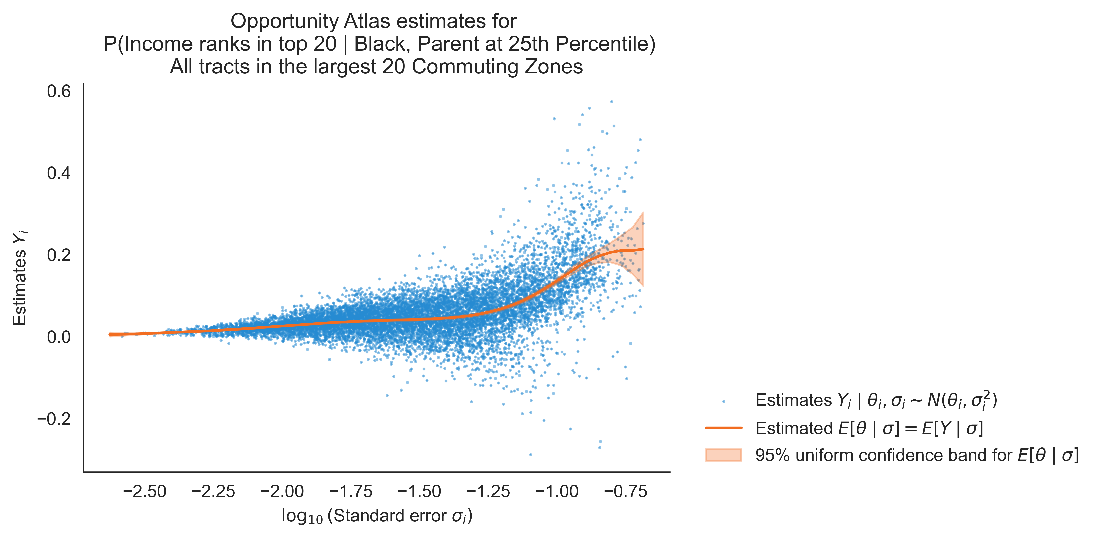
Notes.

All tracts within the largest 20 Commuting Zones (CZs) are shown. Due to the regression specification in Chetty et al. (2020), point estimates of $\theta_{i}\in[0,1]$ do not always lie within $[0,1]$. The orange line plots nonparametric regression estimates of the conditional mean $\mathbb{E}[Y\mid\sigma]=\mathbb{E}[\theta\mid\sigma]\equiv m_{0}(\sigma)$, estimated via local linear regression with automatic bandwidth selection implemented in Calonico et al. (2019). The orange shading shows a 95% uniform confidence band, constructed by the max-$t$ confidence set over 50 equally spaced evaluation points. The confidence band excludes any constant function. See Appendix G for details on estimating conditional moments of $\theta_{i}$ given $\sigma_{i}$. ∎

Figure 1. Scatter plot of $Y_{i}$ against $\log_{10}(\sigma_{i})$ in the Opportunity Atlas

As an empirical matter, prior independence is readily rejected for this measure of economic mobility. Figure 1 plots $Y_{i}$ against $\log_{10}(\sigma_{i})$, as well as a nonparametric regression estimate of $m_{0}(\sigma_{i})\equiv\mathbb{E}[\theta_{i}\mid\sigma_{i}]=\mathbb{E}[Y_{i}\mid\sigma_{i}]$. If $\theta_{i}$ were independent of $\sigma_{i}$, then the true conditional mean function, $m_{0}(\sigma_{i})$, should be constant. Figure 1 shows the contrary—tracts with more imprecisely estimated $Y_{i}$ tend to have higher economic mobility. This correlation is in part through the following channel. Since $\theta_{i}$ is an average outcome for children from poor Black families, tracts with more poor Black families tend to have more precise estimates of $\theta_{i}$. However, they also tend to have lower economic mobility $\theta_{i}$ due to the pernicious effects of residential segregation.

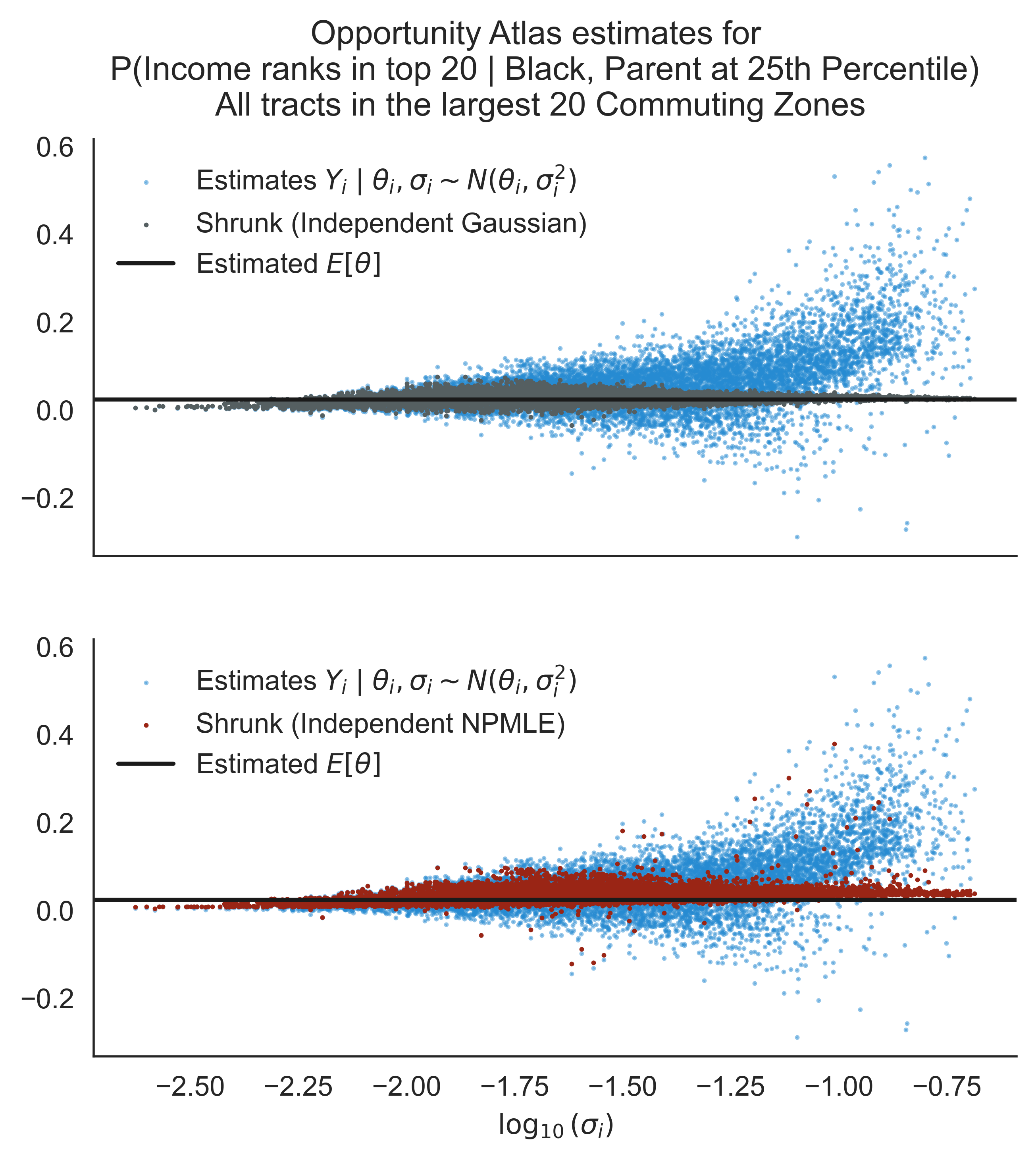
Notes.

The top panel shows posterior mean estimates with independent-gauss shrinkage. The bottom panel shows the same with independent-npmle shrinkage. In the top panel, the estimates for $m_{0},s_{0}^{2}$ are weighted by the precision $1/\sigma_{i}^{2}$ (as in Bergman et al., 2023). Under $\theta_{i}\indep\sigma_{i}$, this weighting scheme improves efficiency of the $(m_{0},s_{0})$-estimates by underweighting noisier $Y_{i}$. ∎

Figure 2. Posterior mean estimates under prior independence

What happens if we apply empirical Bayes methods that assume prior independence here? Figure 2 overlays the empirical Bayes posterior means, computed from independent-gauss and independent-npmle, on the $Y_{i}$-against-$\log\sigma_{i}$ scatterplot. independent-gauss (1) shrinks estimates $Y_{i}$ towards a common estimated mean $\hat{m}_{0}$, depicted as the black line in Figure 2(a), and shrinks noisier estimates more aggressively. When $\sigma_{i}$ and $\theta_{i}$ are positively correlated—as is the case in Figure 2, estimated posterior means under independent-gauss systematically undershoot $\theta_{i}$ for populations with imprecise estimates. Similarly, independent-npmle suffers from the same undershooting, though less so.

This undershooting is particularly problematic for Decision Problem 2 and Decision Problem 3. In these problems, the tracts one would like to select are exactly those with high imprecision $\sigma_{i}$, owing to the positive correlation between $\theta_{i}$ and $\sigma_{i}$. By shrinking these tracts severely towards the estimated common mean, empirical Bayes under prior independence makes suboptimal selections that may underperform screening directly based on $Y_{i}$.

We end this section with a discussion on the plausibility of prior independence in other economic contexts.

Remark 1 (Plausibility of prior independence).

To describe the general channels underlying the potential failure of prior independence, let us write (2) in a different form

$$\sqrt{n_{i}}(Y_{i}-\theta_{i})\overset{d}{\longrightarrow}\mathcal{N}(0,\sigma_{0i}^{2})\quad\text{ where $\sigma_{i}\approx\frac{\sigma_{0i}}{\sqrt{n_{i}}}$}.$$

Expression (1) decomposes the (estimated) standard error into the underlying sample size $n_{i}$ in the micro-data and the asymptotic variance $\sigma_{0i}^{2}$ of the (properly scaled) estimator. Both $n_{i}$ and $\sigma_{0i}$ may predict $\theta_{i}$ in a variety of empirical contexts.

Let us start with the implicit sample sizes $n_{i}$. It is possible that $n_{i}$ is in part determined by $\theta_{i}$, which we loosely term selection. In value-added modeling, $n_{i}$ is the number of observations associated with a provider. It is possible that $n_{i}$ selects on the latent quality $\theta_{i}$ of that provider. For instance, Chandra et al. (2016) find “higher quality hospitals have higher market shares and grow more over time.” If market share and hospital size relate to the underlying sample size $n_{i}$ (e.g. number of patient observations) for estimating hospital value-added, then this suggests non-independence between $\theta_{i}$ and $\sigma_{i}$. As another example, in meta-analysis, suppose $\theta_{i}$ represents the treatment effect of some intervention $i$. If researchers power studies based on informative priors for $\theta_{i}$, then we should observe that interventions with larger conjectured effect sizes have smaller sample sizes $n_{i}$.

Another channel driving the correlation between $n_{i}$ and $\theta_{i}$ can be loosely termed congestion, where $n_{i}$ affects the latent feature $\theta_{i}$. For our primary application, $n_{i}$ represents the number of poor and minority households in a Census tract, and $\theta_{i}$ represents underlying economic or social mobility. Places with more poor and minority households experience white flight and residential segregation (Cutler et al., 1999; Agan and Starr, 2020; Kain, 1968), develop oppressive institutions (Derenoncourt, 2022; Alesina et al., 2001), and worse public goods provision (Laliberté, 2021; Jackson and Mackevicius, 2021; Colmer et al., 2020). These factors contribute to lower economic mobility $\theta_{i}$. Section A.5 contains more examples of violation of prior independence and outlines a model in which selection and congestion effects drive correlation between $n_{i}$ and $\theta_{i}$.

There are also cases where the asymptotic variance $\sigma_{0i}^{2}$ is correlated with $\theta_{i}$. In the context of intergenerational mobility, a parallel literature on the Great Gatsby curve (reviewed by Durlauf et al., 2022) seeks to explain a negative relationship between inequality—which contributes to $\sigma_{0i}^{2}$—and intergenerational mobility. For instance, Becker et al. (2018) posit that parental investment and parental human capital are complements in a child’s skill formation. As a result, parents with higher human capital—and more wealth—invest disproportionately more in their children’s education than parents with lower human capital. This process then produces both inequality and low economic mobility. In other words, places that are more unequal (higher $\sigma_{0i}^{2}$) have lower mobility $\theta_{i}$. $\blacksquare$

2.3. Conditional location-scale relaxation of prior independence

Having argued that (i) prior independence is theoretically suspect and empirically rejected and that (ii) inappropriately imposing it can harm empirical Bayes decision rules, we propose the conditional location-scale model (2.4) as a relaxation. Here, we state (2.4) equivalently as

$$\theta_{i}=m_{0}(\sigma_{i})+s_{0}(\sigma_{i})\tau_{i}\qquad\tau_{i}\mid\sigma_{i}\overset{\mathrm{i.i.d.}}{\sim}G_{0}\qquad\mathbb{E}_{G_{0}}[\tau_{i}]=0\qquad\operatorname{Var}_{G_{0}}(\tau_{i})=1.$$ (2.11)

To estimate $P_{0}$ under this assumption, it suffices to estimate the unknown hyperparameters $(m_{0},s_{0},G_{0})$. Expression (2.11) makes clear that, under the location-scale model, the transformed parameter $\tau_{i}=\frac{\theta_{i}-m_{0}(\sigma_{i})}{s_{0}(\sigma_{i})}$ is independent from $\sigma_{i}$ with distribution $G_{0}$. Applying the same transformation to the data $(Y_{i},\sigma_{i})$ yields transformed estimates $Z_{i}=\frac{Y_{i}-m_{0}(\sigma_{i})}{s_{0}(\sigma_{i})}$ and its standard errors $\nu_{i}=\frac{\sigma_{i}}{s_{0}(\sigma_{i})}$, which obey an analogue of the Gaussian location model (2) in which prior independence holds:

$$Z_{i}\mid\nu_{i},\tau_{i}\sim\mathcal{N}(\tau_{i},\nu_{i}^{2}),\text{ independently across $i$}\text{ and }\tau_{i}\mid\sigma_{i}\sim G_{0}$$

Thus, it is natural to use empirical Bayes methods that assume prior independence on these transformed quantities to estimate $G_{0}$.

This strategy is still infeasible, since the transformation depends on unknown location and scale parameters $\eta_{0}\equiv(m_{0},s_{0})$. Fortunately, these are readily estimable from the data $(Y_{i},\sigma_{i})$, as they only require conditional expectations and variances of $Y$ given $\sigma$:

$$m_{0}(\sigma)=\mathbb{E}[\theta\mid\sigma]=\mathbb{E}[Y\mid\sigma]\quad\text{ and }\quad s_{0}^{2}(\sigma)=\operatorname{Var}(\theta\mid\sigma)=\mathbb{E}[(Y-m_{0}(\sigma))^{2}\mid\sigma]-\sigma^{2}.$$

We then form the estimated transformed data $\hat{Z}_{i},\hat{\nu}_{i}$ as

$$\hat{Z}_{i}=\frac{Y_{i}-\hat{m}(\sigma_{i})}{\hat{s}(\sigma_{i})}\quad\text{and }\quad\hat{\nu}_{i}=\frac{\sigma_{i}}{\hat{s}(\sigma_{i})}.$$

We apply empirical Bayes methods assuming prior independence on $(\hat{Z}_{i},\hat{\nu}_{i})$. This leads to a family of empirical Bayes strategies that we refer to as conditional location-scale empirical Bayes, or close:

1. Nonparametrically estimate $m_{0}(\sigma)=\mathbb{E}[Y\mid\sigma],s_{0}^{2}(\sigma)=\operatorname{Var}(Y\mid\sigma)-\sigma^{2}$.

2. With the estimates $\hat{\eta}=(\hat{m},\hat{s})$, transform the data according to (2.3). Apply empirical Bayes methods with prior independence to estimate $G_{0}$ with some $\hat{G}_{n}$ on the transformed data $(\hat{Z}_{i},\hat{\nu}_{i})$.

3. Having estimated $(\hat{\eta},\hat{G}_{n})$—whose population counterparts $(\eta_{0},G_{0})$ fully describe $P_{0}$ under the conditional location-scale assumption (2.4)—we then form empirical Bayes decision rules as in (2.1).

This procedure produces a family of strategies since $\boxed{\textbf{{close}--{step} {\small 2}}}$ can take different forms. We consider two flavors of close.

2.3.1. close-npmle

To leverage theoretical and computational advances, we will focus on—and recommend—using nonparametric maximum likelihood (npmle) to estimate $G_{0}$. That is, we maximize the log-likelihood of (an estimated version of) the transformed data $Z_{i}$, whose marginal distribution is the convolution $G_{0}\star\mathcal{N}(0,\nu_{i}^{2})$:

$$\hat{G}_{n}\in\operatorname*{arg\,max}_{G\in\mathcal{P}(\mathbb{R})}\frac{1}{n}\sum_{i=1}^{n}\log\int_{-\infty}^{\infty}\varphi\left({\frac{\hat{Z}_{i}-\tau}{\hat{\nu}_{i}}}\right)\frac{1}{\hat{\nu}_{i}}\,G(d\tau).$$

The maximization is over the set of all probability measures on $\mathbb{R}$, $\mathcal{P}(\mathbb{R})$. We note that when the estimated moments $\hat{m},\hat{s}$ are constant functions of $\sigma$, close-npmle estimates the same prior as independent-npmle. In the theoretical literature, under prior independence, independent-npmle is state-of-the-art in terms of computational ease and regret properties. Our results in Section 3 extend some of these favorable properties to close-npmle under the conditional location-scale model.

A simple alternative, which we call close-gauss and think of as a “lite” version of close-npmle, additionally models the shape $G_{0}$ as (standard) Gaussian. We briefly discuss its properties in the following section.

2.3.2. close-gauss

Under $G_{0}\sim\mathcal{N}(0,1)$, the oracle Bayes posterior means are simply

$$\theta^{*}_{i,\mathcal{N}(0,1),\eta_{0}}=\frac{\sigma_{i}^{2}}{s_{0}^{2}(\sigma_{i})+\sigma_{i}^{2}}m_{0}(\sigma_{i})+\frac{s_{0}^{2}(\sigma_{i})}{s_{0}^{2}(\sigma_{i})+\sigma_{i}^{2}}Y_{i}.$$

Equation (2.3.2) is the analogue of the standard shrinkage formula (1), where unconditional means and variances are replaced with their conditional counterparts. As an empirical Bayes strategy, close-gauss then replaces the unknown conditional moments $(m_{0},s_{0})$ with their estimated counterparts. Its properties depend on those of the oracle (2.3.2) it mimics, which we turn to now.

Despite being rationalized under the restrictive assumption $\theta_{i}\mid\sigma_{i}\sim\mathcal{N}(m_{0}(\sigma_{i}),s_{0}^{2}(\sigma_{i}))$, (2.3.2) enjoys strong robustness properties: It is optimal over a restricted class of decision rules and minimax over all decision rules—without imposing (2.4). First, (2.3.2) is the optimal decision rule for estimating $\theta_{i}$ in squared error—solely under the sampling assumption (2)—among the class of decision rules that are linear in $Y_{i}$: $\delta_{i}(Y_{i},\sigma_{i})=a(\sigma_{i})+b(\sigma_{i})Y_{i}$. Second, (2.3.2) is minimax in the sense that it minimizes the worst-case squared error Bayes risk, where an adversary chooses $G_{(1)},\ldots,G_{(n)}$, subjected to the constraint that $G_{(i)}$’s first two moments are $(m_{0}(\sigma_{i}),s_{0}^{2}(\sigma_{i}))$.

However, the Normality assumption does imply that (2.3.2), unlike close-npmle, fails to achieve optimality—in the sense of vanishing regret (2.1)—when the location-scale assumption (2.4) does hold. Since we also show that close-npmle is worst-case robust—though with higher worst-case risk than close-gauss, we recommend close-npmle over close-gauss, unless the researcher is extremely concerned about the misspecification of the location-scale model.

3. Regret results for close-npmle

Recall that we observe $(Y_{i},\sigma_{i})_{i=1}^{n}$, where $(\theta_{i},\sigma_{i})$ satisfies the location-scale assumption (2.4) and $(Y_{i},\theta_{i},\sigma_{i})$ obeys the Gaussian location model (2). Our recommended procedure, close-npmle, transforms the data $(Y_{i},\sigma_{i})$ into $(\hat{Z}_{i},\hat{\nu}_{i})$, with estimated nuisance parameters $\hat{\eta}=(\hat{m},\hat{s})$ for $\eta_{0}=(m_{0},s_{0})$ in $\boxed{\textbf{{close}--{step} {\small 1}}}$. It then estimates the unknown shape parameter $G_{0}$ via npmle (2.3.1) on $(\hat{Z}_{i},\hat{\nu}_{i})_{i=1}^{n}$.

Our leading result shows that close-npmle mimics the oracle Bayesian as well as possible, for the problem of estimation under squared error loss, in the sense that its Bayes regret vanishes at the minimax optimal rate. Our second result connects squared error estimation to Decision Problems 2 and 3 by showing that if an empirical Bayesian has low regret in squared error loss, then they likewise have low regret for Decision Problems 2 and 3.

Since our main result assumes the location-scale model, one may be concerned about potential misspecification of the location-scale model. The last result in this section, 2, bounds the worst-case Bayes risk of an idealized version of close-npmle (i.e. with known $\eta_{0}$ and fixed but misspecified $\hat{G}_{n}$) as a multiple of the minimax risk without assuming (2.4). Thus, even under misspecification, close-npmle does not perform arbitrarily badly relative to the minimax procedure.

The rest of this section states and discusses these results formally. Practitioners who are less interested in the theoretical details are free to skip to Section 4, where we discuss a number of practical considerations.

Remark 2 (Notation).

In what follows, we use the symbol $C$ to denote a generic positive and finite constant which does not depend on $n$. We use the symbol $C_{x}$ to denote a generic positive and finite constant that depends only on $x$, some parameter(s) that describe the problem. Occurrences of the same symbol $C,C_{x}$ may not refer to the same constants. Similarly, for $A_{n},B_{n}\geq 0$, generally functions of $n$, we use $A_{n}\lesssim B_{n}$ to mean that some universal $C$ exists such that $A_{n}\leq CB_{n}$ for all $n$, and we use $A\lesssim_{x}B$ to mean that some universal $C_{x}$ exists such that $A_{n}\leq C_{x}B_{n}$ for all $n$. In logical statements, appearances of $\lesssim$ implicitly prepend “there exists a universal constant” to the statement. For instance, statements like “under certain assumptions, $\operatorname{P}(A_{n}\lesssim B_{n})\geq c_{0}$” should be read as “under certain assumptions, there exists a constant $C>0$ such that for all $n$, $\operatorname{P}(A_{n}\leq CB_{n})\geq c_{0}$.”

Since all expectation or probability statements are with respect to the conditional distribution $P_{0}$ of $\theta_{1:n}\mid\sigma_{1:n}$, going forward, we treat $\sigma_{1:n}$ as fixed and simply write $\mathbb{E}[\cdot],\operatorname{P}(\cdot)$ to denote the expectation and probability over $\theta_{1:n}\mid\sigma_{1:n}\sim P_{0}$. We omit the $P_{0}$ subscript and the conditioning on $\sigma_{1:n}$. $\blacksquare$

3.1. Regret rate in squared error

Since we consider close-npmle in mean-squared error, we specialize and define

$$\mathrm{MSERegret}_{n}(G,\eta) \equiv\frac{1}{n}\sum_{i=1}^{n}(\hat{\theta}_{i,G,\eta}-\theta_{i})^{2}-\frac{1}{n}\sum_{i=1}^{n}\left({\theta_{i}^{*}-\theta_{i}}\right)^{2}$$

$$\theta_{i}^{*}\equiv\theta_{i,P_{0}}^{*}=\mathbb{E}_{P_{0}}[\theta_{i}\mid Y_{i},\sigma_{i}]\quad\hat{\theta}_{i,G,\eta} \equiv\mathbf{E}_{G,\eta}[\theta_{i}\mid Y_{i},\sigma_{i}]\equiv\frac{\int\theta\varphi\left({\frac{Y_{i}-\theta}{\sigma_{i}}}\right)\frac{1}{\sigma_{i}}dG\left({\frac{\theta-m(\sigma_{i})}{s(\sigma_{i})}}\right)}{\int\varphi\left({\frac{Y_{i}-\theta}{\sigma_{i}}}\right)\frac{1}{\sigma_{i}}dG\left({\frac{\theta-m(\sigma_{i})}{s(\sigma_{i})}}\right)}$$

as the excess loss of the empirical Bayes posterior means—obtained by prior $G$ and nuisance parameter estimate $\eta$ for $\eta_{0}$—relative to that of the oracle Bayes posterior means. The Bayes regret for close-npmle in squared error is then the $P_{0}$-expectation of $\mathrm{MSERegret}_{n}$:

$$\mathrm{BayesRegret}_{n}=\mathbb{E}\left[{\mathrm{MSERegret}_{n}(\hat{G}_{n},\hat{\eta})}\right]=\mathbb{E}\left[{\frac{1}{n}\sum_{i=1}^{n}(\theta_{i}^{*}-\hat{\theta}_{i,\hat{G}_{n},\hat{\eta}})^{2}}\right].$$

Equation (3.1) additionally notes that expected $\mathrm{MSERegret}_{n}$ is equal to the expected mean-squared difference between the empirical Bayesian posterior means $\hat{\theta}_{i,\hat{G}_{n},\hat{\eta}}$ and the oracle Bayes posterior means.

We assume that $P_{0}\in\mathcal{P}_{0}$ belongs to some restricted class. Informally speaking, our first main result shows that for some constants $C,\beta>0$ that depend solely on $\mathcal{P}_{0}$, the Bayes regret in squared error decays at the same rate as the maximum estimation error for $\eta_{0}$ squared:

$$\mathrm{BayesRegret}_{n}\leq C(\log n)^{\beta}\max\left({\mathbb{E}\lVert\hat{\eta}-\eta_{0}\rVert_{\infty}^{2},\frac{1}{n}}\right),$$

where we define $\lVert\eta\rVert_{\infty}=\max\left({\lVert m\rVert_{\infty},\lVert s\rVert_{\infty}}\right)$ for $\eta=(m,s).$ This result continues a recent statistics literature on empirical Bayes methods via npmle by characterizing the effect of an estimated nuisance parameter $\hat{\eta}$ in a first step.

Moreover, we show that controlling the Bayes regret is no easier than estimating $m$ in $\lVert\cdot\rVert_{2}$, which is a corresponding lower bound on regret. There exists $c$ such that for any estimator of $\theta_{i}$, its worst-case regret is bounded below

$$\sup_{P_{0}}\mathrm{BayesRegret}_{n}\geq c\inf_{\hat{m}}\sup_{m_{0}}\mathbb{E}\lVert\hat{m}-m_{0}\rVert^{2}_{2}.$$

Since the minimax estimation rates of $\lVert\hat{\eta}-\eta_{0}\rVert_{\infty}$ and of $\lVert\hat{\eta}-\eta_{0}\rVert_{2}$ are the same up to logarithmic factors, we conclude that our regret upper bound is rate-optimal up to logarithmic factors. We now introduce the assumptions on $P_{0}\in\mathcal{P}_{0}$ needed for these results, state the upper and lower bounds, and provide a technical discussion.

3.1.1. Assumptions for regret upper bound

We first assume that $\hat{G}_{n}$ is an approximate maximizer of the log-likelihood on the transformed data $\hat{Z}_{i}$ and $\hat{\nu}_{i}$ satisfying some support restrictions. This is not a restrictive assumption, as the actual maximizers of the log-likelihood function satisfy it.

Assumption 1.

Let $\psi_{i}(Z_{i},\hat{\eta},G)\equiv\log\left({\int_{-\infty}^{\infty}\varphi\left({\frac{\hat{Z}_{i}-\tau}{\hat{\nu}_{i}}}\right)G(d\tau)}\right)$ be the objective function in (2.3.1), ignoring a constant factor $1/\hat{\nu}_{i}$. We assume that $\hat{G}_{n}$ satisfies

$$\frac{1}{n}\sum_{i=1}^{n}\psi_{i}(Z_{i},\hat{\eta},\hat{G}_{n})\geq\sup_{H\in\mathcal{P}(\mathbb{R})}\frac{1}{n}\sum_{i=1}^{n}\psi_{i}(Z_{i},\hat{\eta},H)-\kappa_{n}$$

for tolerance $\kappa_{n}$

$$\kappa_{n}=\frac{2}{n}\log\left({\frac{n}{\sqrt{2\pi}e}}\right).$$

Moreover, we require that $\hat{G}_{n}$ has support points within $[\min_{i}\hat{Z}_{i},\max_{i}\hat{Z}_{i}]$. To ensure that $\kappa_{n}$ is positive, we assume that $n\geq 7=\lceil\sqrt{2\pi}e\rceil$.

We now state further assumptions on the data-generating processes $P_{0}$ beyond (2.4). First, we assume that $G_{0}$ is exponential-tailed with parameter $\alpha$ that controls the thickness of its tails. We state the restriction in an equivalent form of simultaneous moment control.

Assumption 2.

The distribution $G_{0}$ is has zero mean, unit variance, and admits simultaneous moment control with parameter $\alpha\in(0,2]$: There exists a constant $A_{0}>0$ such that for all $p>0$,

$$\left({\mathbb{E}_{\tau\sim G_{0}}[|\tau|^{p}]}\right)^{1/p}\leq A_{0}p^{1/\alpha}.$$

Next, Assumption 3 bounds the variance parameters away from zero and infinity. This is a standard assumption in the literature, maintained likewise by Jiang (2020) and Soloff et al. (2021).

Assumption 3.

The variances $(\sigma_{1:n},s_{0})$ admit lower and upper bounds:

$$\sigma_{\ell}<\sigma_{i}<\sigma_{u}\text{ and }s_{\ell}<s_{0}(\cdot)<s_{u},$$

where $0<\sigma_{\ell},\sigma_{u},s_{0\ell},s_{0u}<\infty$. This implies that $0<\nu_{\ell}\leq\nu_{i}=\frac{\sigma_{i}}{s_{0}(\sigma_{i})}\leq\nu_{u}<\infty$ for some $\nu_{\ell},\nu_{u}$.

Lastly, we require that $m_{0},s_{0}$ satisfies some smoothness restrictions. We also require that $\hat{m},\hat{s}$ satisfy some corresponding regularity conditions.

Assumption 4.

Let $C_{A_{1}}^{p}([\sigma_{\ell},\sigma_{u}])$ be the Hölder class of order $p>0$ with maximal Hölder norm $A_{1}>0$ supported on $[\sigma_{\ell},\sigma_{u}]$.

Definition 1.

For some set $\mathcal{X}\subset\mathbb{R}$ and constant $A>0$, $p>0$, let $C_{A}^{p}(\mathcal{X})$ be the set of continuous functions $f:\mathcal{X}\to\mathbb{R}$ with $\lVert f\rVert_{(p)}\leq A$. The norm $\lVert\cdot\rVert_{(p)}$ is defined as follows. Let $\underline{p}$ be the greatest integer strictly smaller than $p$. Define $$\lVert f\rVert_{(p)}=\max_{k\leq\underline{p}}\sup_{x\in\mathcal{X}}\left|f^{(k)}(x)\right|+\sup_{x,y\in\mathcal{X}}\frac{\left|f^{(\underline{p})}(x)-f^{(\underline{p})}(y)\right|}{|x-y|^{p-\underline{p}}}.$$ We refer to $C_{A}^{p}(\mathcal{X})$ as a Hölder class of order $p$ and $\lVert f\rVert_{(p)}$ as the Hölder norm. We assume that

1. The true conditional moments are Hölder-smooth: $m_{0},s_{0}\in C_{A_{1}}^{p}([\sigma_{\ell},\sigma_{u}])$.

Additionally, let $\beta_{0}>0$ be a constant. Let $\mathcal{V}$ be a set of bounded functions supported on $[\sigma_{\ell},\sigma_{u}]$ that (i) admits the uniform bound $\sup_{f\in\mathcal{V}}\lVert f\rVert_{\infty}\leq C_{A_{1}}$ and (ii) admits the metric entropy bound

$$\log N(\epsilon,\mathcal{V},\lVert\cdot\rVert_{\infty})\leq C_{A_{1},p,\sigma_{\ell},\sigma_{u}}(1/\epsilon)^{1/p}.$$

We assume that the estimators for $m_{0}$ and $s_{0}$, $\hat{\eta}=(\hat{m},\hat{s})$, satisfy the following assumptions.

1. For any $\epsilon>0$, there exists a sufficiently large $C=C(\epsilon)$, independently of $n$, such that for all $n$,

   $$\operatorname{P}\left({\max\left({\lVert\hat{m}-m_{0}\rVert_{\infty},\lVert\hat{s}-s_{0}\rVert_{\infty}}\right)>C(\epsilon)n^{-\frac{p}{2p+1}}(\log n)^{\beta_{0}}}\right)<\epsilon.$$

2. The nuisance estimators take values in $\mathcal{V}$ almost surely: $\operatorname{P}\left({\hat{m}\in\mathcal{V},\hat{s}\in\mathcal{V}}\right)=1$.

3. The conditional variance estimator respects the conditional variance bounds in Assumption 3: $\operatorname{P}\left({\frac{s_{0\ell}}{2}<\hat{s}<2s_{0u}}\right)=1$.

Assumption 4 is a Hölder smoothness assumption on the nuisance parameters $m_{0}$ and $s_{0}$, which is a standard regularity condition in nonparametric regression; our subsequent minimax rate optimality statements are relative to this class. Moreover, it is also a high-level assumption on the quality of the estimation procedure for $(\hat{m},\hat{s})$. Specifically, Assumption 4 expects that the nuisance parameter estimates $\hat{m}$ and $\hat{s}$ are rate-optimal up to logarithmic factors (Stone, 1980). Assumption 4 also expects that the nuisance parameter estimates belong to a class $\mathcal{V}$ with the same metric entropy behavior as the Hölder class $C_{A_{1}}^{p}([\sigma_{\ell},\sigma_{u}])$.

Assumptions 2, 4, and 3 specify a class of distributions $\mathcal{P}_{0}$ and nuisance estimators $\hat{\eta}$ indexed by a set of hyperparameters $\mathcal{H}=(\sigma_{\ell},\sigma_{u},s_{\ell},s_{u},A_{0},A_{1},\alpha,\beta_{0},p).$ Our subsequent theoretical results are finite sample, with implicit constants dependent on these hyperparameters $\mathcal{H}$. To review, $(\sigma_{\ell},\sigma_{u},s_{\ell},s_{u})$ are bounds on the variances $(\sigma_{i}^{2},s^{2}(\sigma_{i}))$; $(A_{0},\alpha)$ control the tails of $G_{0}$; and $(A_{1},p)$ control the smoothness of $\eta_{0}$; and $\beta_{0}$ is the power of the log factor in the $\lVert\cdot\rVert_{\infty}$ estimation rate for $\eta_{0}$.

3.1.2. Regret results

Consider the following “good event,” indexed by $C>0$,

$$\mathbf{A}_{n}(C)\equiv\left\{{\lVert\hat{\eta}-\eta_{0}\rVert_{\infty}\leq Cn^{-\frac{p}{2p+1}}(\log n)^{\beta_{0}}}\right\}.$$

$\mathbf{A}_{n}$ indicates that the nuisance parameter estimates satisfy some rate in $\lVert\cdot\rVert_{\infty}$. Our main result derives a convergence rate for the expected MSE regret conditional on this good event $\mathbf{A}_{n}(C).$

Theorem 1.

Assume Assumptions 4, 2, 3, and 1 hold. Then, for any $\delta\in(0,\frac{1}{2})$, there exists universal constants $C_{1,\mathcal{H},\delta}>0$ and $C_{0,\mathcal{H},\delta}>0$ such that (i) $\operatorname{P}(\mathbf{A}_{n}(C_{1,\mathcal{H},\delta}))\geq 1-\delta$ and that (ii) the expected regret conditional on $\mathbf{A}_{n}(C_{1,\mathcal{H},\delta})$ is dominated by the rate function

$$\mathbb{E}\left[{\mathrm{MSERegret}_{n}(\hat{G}_{n},\hat{\eta})\mid\mathbf{A}_{n}(C_{1,\mathcal{H},\delta})}\right]\leq C_{0,\mathcal{H},\delta}n^{-\frac{2p}{2p+1}}(\log n)^{\frac{2+\alpha}{\alpha}+3+2\beta_{0}}.$$

If the event $\mathbf{A}_{n}(C)$ is sufficiently likely, we can control expected regret on the bad event $\mathbf{A}^{\mathrm{C}}_{n}$ as well. In Appendix G, we verify that local linear regression satisfies a weakening of these assumptions that are also sufficient for the conclusion of 1.

Corollary 1.

Assume the same setting as Theorem 1. Suppose, additionally, for all sufficiently large $C_{1,\mathcal{H}}>0$, $\operatorname{P}(\mathbf{A}_{n}(C_{1,\mathcal{H}}))\geq 1-n^{-2}.$ Then, there exists a constant $C_{0,\mathcal{H}}>0$ such that the expected regret is dominated by the rate function

$$\mathrm{BayesRegret}_{n}=\mathbb{E}\left[{\mathrm{MSERegret}_{n}(\hat{G}_{n},\hat{\eta})}\right]\leq C_{0,\mathcal{H}}n^{-\frac{2p}{2p+1}}(\log n)^{\frac{2+\alpha}{\alpha}+3+2\beta_{0}}.$$

We can show a corresponding lower bound on the Bayes regret—i.e., a lower bound on the worst-case Bayes regret when an adversary picks $G_{0},\eta_{0}$—by showing that any good posterior mean estimate $\hat{\theta}_{i}$ implies a good estimate $\hat{m}(\sigma_{i})$ for $m_{0}$. Minimax lower bounds for estimation of $m_{0}$ then imply lower bounds for estimation of the oracle posterior means $\theta_{i}^{*}$.

Theorem 2.

Fix a set of valid hyperparameters $\mathcal{H}=(\sigma_{\ell},\sigma_{u},s_{\ell},s_{u},A_{0},A_{1},\alpha,\beta_{0},p)$ for Assumptions 2, 4, and 3. Let $\mathcal{P}(\mathcal{H},\sigma_{1:n})$ be the set of distributions $P_{0}$ on support points $\sigma_{1:n}$ which satisfy (2.4) and Assumptions 2, 4, and 3 corresponding to $\mathcal{H}$. For a given $P_{0}$, let $\theta_{i}^{*}=\mathbb{E}_{P_{0}}[\theta_{i}\mid Y_{i},\sigma_{i}]$ denote the oracle posterior means. Then there exists a constant $c_{\mathcal{H}}>0$ such that the worst-case Bayes regret of any estimator exceeds $c_{\mathcal{H}}n^{-\frac{2p}{2p+1}}$:

$$\inf_{\hat{\theta}_{1:n}}\sup_{\begin{subarray}{c}\sigma_{1:n}\in(\sigma_{\ell},\sigma_{u})\\ P_{0}\in\mathcal{P}(\mathcal{H},\sigma_{1:n})\end{subarray}}\mathbb{E}_{P_{0}}\left[{\frac{1}{n}\sum_{i=1}^{n}(\hat{\theta}_{i}-\theta_{i})^{2}-(\theta_{i}^{*}-\theta_{i})^{2}}\right]\geq c_{\mathcal{H}}n^{-\frac{2p}{2p+1}},$$

where the infimum is taken over all (possibly randomized) estimators of $\theta_{1:n}$.

As a result, the rate (1) is optimal up to logarithmic factors. The additional logarithmic factors are partly the price of having to estimate $G_{0}$ via npmle and partly deficiencies in the proof of Theorem 1. In any case, this cost is not substantial.

The regret upper bounds Theorems 1 and 1 are finite-sample statements. As a result, they hold uniformly over all distributions $P_{0}$ satisfying Assumptions 4, 2, and 3 delineated by the problem parameters $\mathcal{H}$. However, the usefulness of Theorems 1 and 1 still lies in the convergence rate, as the constants implied by the proofs are not sharp.

These regret upper bounds readily extend to the case where covariates are present and the location-scale assumption is with respect to the additional covariates $X_{i}$:

$$\theta_{i}\mid\sigma_{i},X_{i}\sim G_{0}\left({\frac{\theta_{i}-m_{0}(X_{i},\sigma_{i})}{s_{0}(X_{i},\sigma_{i})}}\right),$$

under assumption on $m_{0},s_{0},\hat{m},\hat{s}$ analogous to Assumption 4. Of course, the resulting convergence rate would suffer from the curse of dimensionality, and the term $n^{-\frac{2p}{2p+1}}$ would be replaced with $n^{-\frac{2p}{2p+1+d}}$, where $d$ is the dimension of $X$.

Taken together, 1 and 2 are strong statistical optimality guarantees for close-npmle in the canonical problem of estimation with squared error loss. That is, the worst-case performance gap of close-npmle relative to the oracle contracts at the best possible rate, meaning that close-npmle mimics the oracle as well as possible.

For interested readers, we provide an overview of the proof of our main result Theorem 1 in the following remark. A more detailed walkthrough is in Section C.3.

Remark 3 (Informal discussion of the proof for Theorem 1).

Regret results assuming prior independence are established by Soloff et al. (2021) and Jiang (2020), and we build on these results for Theorem 1. Applied to $(Z_{i},\nu_{i},\tau_{i})$, these results state that (i) approximate maximizers $\tilde{G}_{n}$ of the (infeasible) log-likelihood $\Psi_{n}(\eta_{0},G)\equiv\frac{1}{n}\sum_{i}\psi_{i}(Z_{i},\eta_{0},G)$ are close to $G_{0}$ in terms of the average Hellinger distance of the induced densities of $Z_{i}$

$$\overline{h}^{2}(f_{\tilde{G}_{n},\bm{\cdot}},f_{G_{0},\bm{\cdot}})=\frac{1}{n}\sum_{i=1}^{n}h^{2}\left({\mathcal{N}(0,\nu_{i}^{2})\star\tilde{G}_{n},\mathcal{N}(0,\nu_{i}^{2})\star G_{0}}\right),\quad h^{2}(f,g)=1-\int_{-\infty}^{\infty}\sqrt{f(x)g(x)}\,dx$$

and (ii) if $\overline{h}^{2}(f_{\tilde{G}_{n},\bm{\cdot}},f_{G_{0},\bm{\cdot}})$ is small, then posterior means for $\tau_{i}$ under $\tilde{G}_{n}$ are close to posterior means under $G_{0}$ in squared error.

Our results extend this argument by accommodating the fact that $\eta_{0}$ is unknown and must be estimated with $\hat{\eta}$. To apply (ii) in the literature, we would like to show that (i’) $\hat{G}_{n}$—an approximate maximizer of the feasible log-likelihood $\Psi_{n}(\hat{\eta},G)=\frac{1}{n}\sum_{i}\psi_{i}(Z_{i},\hat{\eta},G)$—is close to $G_{0}$ in terms of $\overline{h}^{2}(\cdot,\cdot)$. This is not a straightforward task and is the most intricate part of our argument. To show (i’), we prove a lower bound for the likelihood $\Psi_{n}(\eta_{0},\hat{G}_{n})$ (Theorem D.1) and modify (i) suitably to accommodate our likelihood lower bound (Theorem E.1).

To lower bound $\Psi_{n}(\eta_{0},\hat{G}_{n})$, we relate the two likelihoods by linearization (formally, see (D.4)):

$$\Psi_{n}(\hat{\eta},\hat{G}_{n})-\Psi_{n}(\eta_{0},\hat{G}_{n})\approx\frac{1}{n}\sum_{i=1}^{n}\frac{\partial{\psi_{i}(Z_{i},\eta_{0},\hat{G}_{n})}}{\partial{\eta}}\underbrace{(\hat{\eta}(\sigma_{i})-\eta_{0}(\sigma_{i}))}_{\leq\lVert\hat{\eta}-\eta_{0}\rVert_{\infty}}.$$

Since $\hat{G}_{n}$ approximately maximizes the feasible likelihood $\Psi_{n}(\hat{\eta},\cdot)$, $\Psi_{n}(\hat{\eta},\hat{G}_{n})$ is large by construction. Thus, if we can show that the right-hand side is small, then the infeasible likelihood $\Psi_{n}(\eta_{0},\hat{G}_{n})$ would also be large. To obtain the rate (1), it is important to show that the right-hand side vanishes strictly faster than $\lVert\hat{\eta}-\eta_{0}\rVert_{\infty}$. To do so, we additionally need to show that the average derivative $\frac{1}{n}\sum_{i}\partial\psi_{i}(Z_{i},\eta_{0},\hat{G}_{n})/\partial\eta$ is small. Without it, we would obtain a worse squared error regret rate of the form $n^{-\frac{p}{2p+1}}(\log n)^{\beta}$.

In particular, we manage to relate this term to the average Hellinger distance (see Lemmas D.1 and D.2)

$$\left|\frac{1}{n}\sum_{i=1}^{n}\frac{\partial{\psi_{i}(Z_{i},\eta_{0},\hat{G}_{n})}}{\partial{\eta}}\right|\lesssim(\log n)^{\gamma}\overline{h}(f_{\hat{G}_{n},\bm{\cdot}},f_{G_{0},\bm{\cdot}})\text{, for some $\gamma>0$.}$$

Loosely, this is because the population score in $\eta$ is mean-zero, $\mathbb{E}[\partial\psi_{i}(Z,\eta_{0},G_{0})/\partial\eta]=0$. Thus if $\hat{G}_{n}$ is close to $G_{0}$, then the sample score evaluated at $\hat{G}_{n}$ should also be approximately zero. This is a key step in Appendix D.

This bound for $\Psi_{n}(\eta_{0},\hat{G}_{n})$ creates an additional complication when attempting to apply the claim (i). The claim (i) upper bounds the Hellinger distance $\overline{h}(f_{\tilde{G}_{n},\bm{\cdot}},f_{G_{0},\bm{\cdot}})$ using a lower bound for $\Psi_{n}(\eta_{0},\tilde{G}_{n})$. However, now our lower bound for the likelihood $\Psi_{n}(\eta_{0},\hat{G}_{n})$ itself depends on $\overline{h}(f_{\hat{G}_{n},\bm{\cdot}},f_{G_{0},\bm{\cdot}})$, and so we cannot apply (i) directly. The proof for (i’) additionally modifies the argument for (i) to accommodate our likelihood bound (Appendix E). $\blacksquare$

So far, our regret guarantees are only about estimation in squared error (Decision Problem 1). In the next subsection, we analyze regret for empirical Bayes decision rules targeted to the ranking-related problems (Decision Problems 2 and 3), and relate their performances to those for Decision Problem 1.

3.2. Other decision objectives and relation to squared-error loss

Notably, the oracle Bayes decision rules $\bm{\delta}^{\star}$ in Decision Problems 2 and 3 depend solely on the vector of oracle Bayes posterior means $\theta_{1:n}^{*}$. Therefore, for these problems, the natural empirical Bayes decision rules simply replace oracle Bayes posterior means, $\theta_{i}^{*}$, with empirical Bayes ones, $\hat{\theta}_{i}$, in the oracle decision rules. For instance, if one is comfortable with the prior estimated by close-npmle, then the corresponding decision rules for Decision Problems 2 and 3 threshold based on estimated posterior means under close-npmle.

In these problems, $\mathrm{BayesRegret}_{n}$ (2.1) is equal to the expected risk gap between using the feasible decision rules $\hat{\bm{\delta}}$ and the oracle decision rules $\bm{\delta}^{\star}$. To specialize, we let $\mathrm{UMRegret}_{n}$ denote $\mathrm{BayesRegret}_{n}$ for Decision Problem 2 and we let $\mathrm{TopRegret}_{n}^{(m)}$ denote $\mathrm{BayesRegret}_{n}$ for Decision Problem 3. The following result relates $\mathrm{UMRegret}_{n}$ and $\mathrm{TopRegret}_{n}^{(m)}$ to $\mathrm{MSERegret}_{n}$.

Theorem 3.

Suppose (2) holds, but (2.4) may or may not hold. Let $\hat{\delta}_{i}$ be the plug-in decisions with any vector of estimates $\hat{\theta}_{i}$, not necessarily from close-npmle. We have the following inequalities on the expected regret corresponding to the decision rules $\hat{\delta}_{i}$:

1. For utility maximization by selection,

   $$\mathbb{E}[\mathrm{UMRegret}_{n}]\leq\left({\mathbb{E}\left[{\frac{1}{n}\sum_{i=1}^{n}(\hat{\theta}_{i}-\theta_{i}^{*})^{2}}\right]}\right)^{1/2}.$$

2. For top-$m$ selection,

   $$\mathbb{E}[\mathrm{TopRegret}_{n}^{(m)}]\leq 2\sqrt{\frac{n}{m}}\left({\mathbb{E}\left[{\frac{1}{n}\sum_{i=1}^{n}(\hat{\theta}_{i}-\theta_{i}^{*})^{2}}\right]}\right)^{1/2}.$$

Theorem 3 shows that the two decision problems utility maximization by selection and top-$m$ selection are easier than estimating the oracle Bayesian posterior means. As a result, our convergence rates from Theorems 1 and 1 also upper bound regret rates for these two decision problems, rendering the regret rates more immediately useful for policy problems. In particular, for $m/n\asymp 1$, both regret rates (1) and (2) are of the form $n^{-p/(2p+1)}(\log n)^{\frac{2+\alpha}{2\alpha}+3/2+\beta_{0}}=o(1)$ under 1. Thus, the performance of the empirical Bayes decision rule approximates that of the oracle at approximately the rate $O(n^{-p/(2p+1)})$. However, the actual performance of close-npmle for Decision Problems 2 and 3 may be better than predicted by Theorem 3. The speed at which regret converges, as implied by Theorem 3, might not be tight, though it is competitive with recent results.

Recall that we can think of top-$m$ selection as the decision problem in Bergman et al. (2023). The utility function represents the expected mobility of a mover, assuming that the mover moves randomly into one of the high mobility Census tracts. Our proof of Theorem 3 in Section A.2 allows for a slightly more general decision problem. Suppose the decision now is to provide a full ranking of Census tracts for potential movers and maximize the expected mobility for a mover. Suppose that the probability that a mover moves to a tract depends decreasingly and solely on the tract’s rank. To be more concrete, suppose the mover has probability $\pi_{1}$ of moving to the highest-ranked tract, $\pi_{2}$ to the second-highest, and so forth. Then, with the same argument, the corresponding regret is dominated by $2\sqrt{n\sum_{i=1}^{n}\pi_{i}^{2}}\cdot\left({\mathbb{E}\left[{\frac{1}{n}\sum_{i=1}^{n}(\hat{\theta}_{i}-\theta_{i}^{*})^{2}}\right]}\right)^{1/2}$, which generalizes (2).

3.3. Robustness to the location-scale assumption (2.4)

We prove our regret upper and lower bounds imposing the location-scale model (2.4). This is an optimistic assessment of the performance of close-npmle. While (2.4) nests prior independence, it may still be misspecified. We now consider the worst-case behavior of close-npmle without the location-scale assumption. Section A.7.3 additionally discusses an interpretation of close-npmle under misspecification of (2.4).

We will do so by considering an idealized version of the procedure. So long as $\theta_{i}\mid\sigma_{i}$ has two moments, $\eta_{0}(\cdot)=(m_{0}(\cdot),s_{0}(\cdot))$ are well-defined as conditional moments of $\theta_{i}\mid\sigma_{i}$ without imposing the location-scale assumption. We will assume that $m_{0},s_{0}$ are known. Without the location-scale model, $G_{0}$ is ill-defined, but we will assume that we obtain some pseudo-true value $G_{0}^{*}$ that has zero mean and unit variance. This is a reasonable condition to impose, since every conditional prior distribution $\tau_{i}\mid\sigma_{i}$ obeys this moment constraint. Thus, for estimating $\tau_{i}=\frac{\theta_{i}-m_{0}(\sigma_{i})}{s_{0}(\sigma_{i})}$, whose true prior is $\tau_{i}\mid\sigma_{i}\sim G_{i}$, this idealized procedure uses some misspecified prior $G_{0}^{*}\neq G_{i}$, which does have the correct first two moments. Chen (2023) shows that the worst-case risk for estimating $\tau_{i}$ is uniformly bounded, over arbitrary choices of $\nu>0$ and $G,G_{0}^{*}$ with zero mean and unit variance: Let $\mathcal{M}$ be the set of mean-zero, variance-one distributions, then

$$\overline{R}_{\mathrm{B}}\equiv\sup\left\{{\mathbb{E}_{\tau\sim G,Z\sim\mathcal{N}(\tau,\nu^{2})}\left[{(\mathbf{E}_{G_{0}^{*}}[\tau\mid Z,\nu]-\tau)^{2}}\right]:G_{0}^{*}\in\mathcal{M},G\in\mathcal{M},\nu>0}\right\}<\infty.$$

Hence, the misspecification of $G_{0}^{*}$ does not cause unbounded risk. Translating this result to the problem of estimating $\theta_{i}$ in squared error, we arrive at the following corollary.

Corollary 2.

Under (2) but not (2.4), assume the conditional distribution $\theta_{i}\mid\sigma_{i}$ has mean $m_{0}(\sigma_{i})$ and variance $s_{0}^{2}(\sigma_{i})$. Denote the set of distributions of $\theta_{1:n}\mid\sigma_{1:n}$ which obey these restrictions as $\mathcal{P}(m_{0},s_{0})$. Let $\hat{\theta}_{i,G_{0}^{*},\eta_{0}}$ denote the posterior mean estimates with a pseudo-true prior which obeys a location-scale model $P^{*}\left({\theta_{i}\leq t\mid\sigma_{i}}\right)=G_{0}^{*}\left({\frac{t-m_{0}(\sigma_{i})}{s_{0}(\sigma_{i})}}\right).$ Assume $G_{0}^{*}$ has zero mean and unit variance. Assume that $G_{0}^{*}$ is non-random. Then, for any $P_{0}\in\mathcal{P}(m_{0},s_{0})$,

$$\mathbb{E}_{P_{0}}\left[{\frac{1}{n}\sum_{i=1}^{n}(\hat{\theta}_{i,G_{0}^{*},\eta_{0}}-\theta_{i})^{2}}\right]\leq\overline{R}_{\mathrm{B}}\frac{1}{n}\sum_{i=1}^{n}s_{0}^{2}(\sigma_{i}).$$

Let $\hat{\theta}_{i}$ be some (possibly randomized) estimator of $\theta_{i}$, which may depend on the data $(Y_{i},\sigma_{i})_{i=1}^{n}$ and $(m_{0},s_{0})$. Suppose additionally that $\sigma_{\ell}=\min_{i}\sigma_{i}>0$ and $s_{u}=\max_{i}s(\sigma_{i})<\infty$. Then, the worst-case risk of $\hat{\theta}_{i}$ is at least

$$\sup_{P_{0}\in\mathcal{P}(m_{0},s_{0})}\mathbb{E}_{P_{0}}\left[{\frac{1}{n}\sum_{i=1}^{n}(\hat{\theta}_{i}-\theta_{i})^{2}}\right]\geq\frac{1}{n}\sum_{i=1}^{n}\frac{\sigma_{i}^{2}}{\sigma_{i}^{2}+s_{0}^{2}(\sigma_{i})}s_{0}^{2}(\sigma_{i})\geq\frac{1}{1+s_{u}^{2}/\sigma_{\ell}^{2}}\frac{1}{n}\sum_{i=1}^{n}s_{0}^{2}(\sigma_{i}).$$

2 shows that an oracle version of close-npmle has finite worst-case risk, scaling like $\overline{R}_{\mathrm{B}}\frac{1}{n}\sum_{i=1}^{n}s_{0}^{2}(\sigma_{i})$. It also shows that any procedure must incur worst-case risk at least $c\frac{1}{n}\sum_{i=1}^{n}s_{0}^{2}(\sigma_{i})$ for some $c>0$. We thus interpret 2 as a robustness guarantee on close-npmle, as it shows that close-npmle approximates some ideal procedure whose worst-case behavior is within a constant multiple of the minimax procedure.

4. Practical considerations when (not) applying close

4.1. A detailed recipe

We now describe the implementation of close-npmle in more detail, following our previous outline in $\boxed{\textbf{{close}--{step} {\small 1}}}$, $\boxed{\textbf{{close}--{step} {\small 2}}}$, and $\boxed{\textbf{{close}--{step} {\small 3}}}$. We emphasize that, in practice, these are implemented in accompanying software; our discussion here is just an overview of what goes on under the hood.

The first step $\boxed{\textbf{{close}--{step} {\small 1}}}$ estimates the conditional moments $\eta_{0}=(m_{0},s_{0})$ nonparametrically. Since the two conditional moments can be written as conditional expectations

$$m_{0}(\sigma) =\mathbb{E}[\theta\mid\sigma]=\mathbb{E}[Y\mid\sigma]$$

$$s_{0}^{2}(\sigma) =\operatorname{Var}(\theta\mid\sigma)=\mathbb{E}[(Y-m_{0}(\sigma))^{2}\mid\sigma]-\sigma^{2},$$ (4.1)

we can estimate them accordingly with off-the-shelf methods (e.g., local polynomial kernel smoothing methods implemented by Calonico et al., 2019). Specifically, estimating $m_{0}$ with $\hat{m}$ is directly a nonparametric regression of $Y_{i}$ on $\sigma_{i}$. Estimating $s_{0}^{2}(\cdot)$ can be operationalized by first nonparametrically regressing $(Y_{i}-\hat{m}(\sigma_{i}))^{2}$ on $\sigma_{i}$, and then subtracting off $\sigma_{i}^{2}$. This is a plug-in estimator for $s_{0}^{2}$, as it replaces quantities in (4.1) with their empirical counterparts.

A wrinkle is that the plug-in estimate $\hat{s}$ may be negative. Truncating $\hat{s}$ at zero results in observations whose estimated prior variances $\hat{s}^{2}(\sigma_{i})=0$. These observations also have implied $\hat{\nu}_{i}=\infty$. For these observations, an empirical Bayesian taking $\hat{s}^{2}(\sigma_{i})=0$ at face value has degenerate priors at $\hat{m}(\sigma_{i})$. Since observations with $\nu_{i}=\infty$ do not contribute to the likelihood objective for npmle, dropping observations with $\hat{s}^{2}(\sigma_{i})=0$ from the npmle estimation and setting the estimated posterior mean for those observations to $\hat{m}(\sigma_{i})$ is consistent with what close-npmle instructs. In our experience, this simple approach does not appear to affect performance. Nevertheless, in Appendix G, we propose a heuristic but data-driven truncation rule, borrowing from a statistics literature on estimating non-centrality parameters for non-central $\chi^{2}$ distributions (Kubokawa et al., 1993). Appendix G also discusses tuning parameter selection for estimating $(m_{0},s_{0})$ and verifies that our local linear regression estimators satisfy the regularity conditions in Section 3.

Next, in the second step $\boxed{\textbf{{close}--{step} {\small 2}}}$, we form the transformed estimates $\hat{Z}_{i}=\frac{Y_{i}-\hat{m}(\sigma_{i})}{\hat{s}(\sigma_{i})}$ and the transformed standard errors $\hat{\nu}_{i}=\frac{\sigma_{i}}{\hat{s}(\sigma_{i})}$. We then estimate the npmle on the data $(\hat{Z}_{i},\hat{\nu}_{i})$ by maximizing (2.3.1). In practice, we approximate the infinite-dimensional optimization problem (2.3.1) with a finite-dimensional one, by discretizing distributions on a grid. To be precise, let $\min_{i}\hat{Z}_{i}=\tau_{(1)}\leq\cdots\leq\tau_{(J)}=\max_{i}\hat{Z}_{i}$ be a pre-specified grid of points, not necessarily equally spaced, and denote it by $\bm{\tau}$. The feasible version of (2.3.1) maximizes the concave program $\pi^{\star}\equiv\max_{\pi\in\mathbb{R}^{J}_{\geq 0},\pi^{\prime}1=1}\sum_{i=1}^{n}\log\left({\sum_{j=1}^{J}\pi_{j}\varphi\left({\frac{\hat{Z}_{i}-\tau_{(j)}}{\hat{\nu}_{i}}}\right)}\right).$ The estimated npmle $\hat{G}_{n}$ is a discrete distribution with support points $\tau_{(j)}$ and corresponding masses $\pi_{j}^{\star}$.

Finally, given the estimate $\hat{G}_{n}=(\bm{\tau},\pi^{\star})$, we can compute empirical Bayes decision rules by minimizing posterior expected loss to implement $\boxed{\textbf{{close}--{step} {\small 3}}}$. Since $\hat{G}_{n}$ is a discrete distribution, the posterior for $\tau_{i}$ is given by the probability mass function

$$\operatorname{P}_{\hat{G}_{n}}(\tau_{i}=\tau_{(j)}\mid\hat{Z}_{i}=z,\hat{\nu}_{i}=\nu)\propto\pi^{\star}_{j}\exp\left({-\frac{1}{2\nu^{2}}(z-\tau_{(j)})^{2}}\right),$$

normalized so that the probabilities sum to 1. This probability mass function can be plugged into (2.1) to compute the empirical Bayes decision rule for any loss function $L$.

4.2. When does relaxing prior independence matter?

When prior independence holds, close-npmle is the same as independent-npmle, up to the estimation of the constant conditional moments $(m_{0}(\cdot),s_{0}(\cdot))$. Since close-npmle has to estimate the conditional moments, we expect it to underperform independent-npmle. Though, since the location-scale assumption (2.4) strictly generalizes prior independence, we do not expect close-npmle to underperform by much in large samples.

When prior independence does not hold, but when the conditional location-scale model (2.4) approximately holds, we expect close to outperform methods that assume prior independence. Qualitatively speaking, if $(m_{0},s_{0})$ are not constant, we expect the improvement of close-methods to be large when large portions of the unconditional signal variance $\operatorname{Var}(\theta_{i})$ is attributable to the conditional expectation. Since we can decompose

$$\operatorname{Var}(\theta_{i})=\mathbb{E}[s_{0}^{2}(\sigma_{i})]+\operatorname{Var}(m_{0}(\sigma_{i})),$$

we expect the improvement of close-methods to be large when the variance of the conditional expectation $\operatorname{Var}(m_{0}(\sigma_{i}))$ is large compared to $\mathbb{E}[s_{0}^{2}(\sigma_{i})]$. Intuitively, this is the case when $\sigma_{i}$ is highly predictive of $\theta_{i}$. Whether this is the case can be easily checked by plotting $Y_{i}$ against $\sigma_{i}$, as in Figure 1, and inspecting the estimated conditional moments.

Finally, when the conditional distributions $\theta_{i}\mid\sigma_{i}$ are non-Gaussian, and in particular when they are discrete, skewed, or thick-tailed, we expect close-npmle to additionally outperform independent-gauss due to not assuming Normality. When the conditional priors are Gaussian, estimating it via the npmle pays a statistical price, but we theoretically and empirically observe that the price is not large. Admittedly, it is often difficult to diagnose whether the underlying conditional distributions $\theta_{i}\mid\sigma_{i}$ have these properties, since we only observe $(Y_{i},\sigma_{i})$. Likewise, so far the discussion in this subsection is heuristic. To be more certain of the extent of improvement of close-npmle over other empirical Bayes methods, it is helpful to have out-of-sample validation. The next subsection proposes a minor extension of Oliveira et al. (2021), which allows for an unbiased estimate of loss and serves as a validation procedure.

4.3. A formal validation procedure via coupled bootstrap

Consider $(Y_{i},\sigma_{i})$ where $Y_{i}\mid\sigma_{i},\theta_{i}\sim\mathcal{N}(\theta_{i},\sigma_{i}^{2})$. For some $\omega>0$ and a random independent Gaussian noise $W_{i}\sim\mathcal{N}(0,1)$, consider adding to $Y_{i}$ and subtracting from $Y_{i}$ some scaled version of $W_{i}$:

$$Y_{i}^{(1)}=Y_{i}+\sqrt{\omega}\sigma_{i}W_{i}\quad Y_{i}^{(2)}=Y_{i}-\frac{1}{\sqrt{\omega}}\sigma_{i}W_{i}.$$

Oliveira et al. (2021) call $(Y_{i}^{(1)},Y_{i}^{(2)})$ the coupled bootstrap draws. Observe that the two couple bootstrap draws are conditionally independent:

$$\begin{bmatrix}Y_{i}^{(1)}\\ Y_{i}^{(2)}\end{bmatrix}\mid\theta_{i},\sigma_{i}^{2}\sim\mathcal{N}\left({\begin{bmatrix}\theta_{i}\\ \theta_{i}\end{bmatrix},\begin{bmatrix}(1+\omega)\sigma_{i}^{2}&0\\ 0&(1+\omega^{-1})\sigma_{i}^{2}\end{bmatrix}}\right).$$

The conditional independence allows us to use $Y_{i}^{(2)}$ as an out-of-sample validation for decision rules computed based on $Y_{i}^{(1)}$. We will denote their marginal variances by $\sigma_{i,(1)}^{2}$ and $\sigma_{i,(2)}^{2}$.

It is helpful to think of $Y_{i}^{(1)}$ as training data and $Y_{i}^{(2)}$ as testing data. In fact, the coupled bootstrap precisely emulates sample-splitting on the micro-data. To see that, suppose $Y_{i}=\frac{1}{n_{i}}\sum_{j=1}^{n}Y_{ij}$ is a sample mean of i.i.d. micro-data $\left\{{Y_{ij}:j=1,\ldots,n_{i}}\right\}$. Suppose we split the micro-data $\left\{{Y_{ij}:j=1,\ldots,n_{i}}\right\}$ into a training set and a testing set, with proportions $\frac{1}{\omega+1}$ and $\frac{\omega}{\omega+1}$, respectively. Let $Y_{i}^{(1)}$ and $Y_{i}^{(2)}$ be the training and testing set sample means, respectively. Then the central limit theorem implies that, approximately,

$$Y_{i}^{(1)}\mid\theta_{i},\sigma_{i}^{2}\sim\mathcal{N}\left({\theta_{i},(1+\omega)\sigma_{i}^{2}}\right)\quad Y_{i}^{(2)}\mid\theta_{i},\sigma_{i}^{2}\sim\mathcal{N}\left({\theta_{i},(1+\omega^{-1})\sigma_{i}^{2}}\right)$$

independently. Note that the two representations (4.3) and (4.3) are equivalent, and hence coupled bootstrap emulates sample-splitting. For instance, coupled bootstrap with a value of $\omega=1/9$ is statistically equivalent to splitting the micro-data with a 90-10 train-test split.

Just as we can perform out-of-sample validation with sample-splitting on the micro-data, we can also do so with the coupled bootstrap emulation of sample-splitting. The following proposition formalizes this and states unbiased estimators for the loss of these decision rules, as well as their accompanying standard errors.

Table 1. Unbiased estimators for loss of decision rules and associated conditional variance expressions (Lemma 1)

Problem	Unbiased estimator of loss, $T\left({Y_{1:n}^{(2)},\bm{\delta}}\right)$	$\operatorname{Var}\left({T\left({Y_{1:n}^{(2)},\bm{\delta}}\right)\mid\mathcal{F}}\right)$
Decision Problem 1	$\frac{1}{n}\sum_{i=1}^{n}\left({Y^{(2)}_{i}-\delta_{i}(Y_{1:n}^{(1)})}\right)^{2}-\sigma_{i,(2)}^{2}$	$\frac{1}{n^{2}}\sum_{i=1}^{n}\operatorname{Var}\left({(Y_{i}^{(2)}-\delta_{i}(Y_{1:n}^{(1)}))^{2}\mid\mathcal{F}}\right)$
Decision Problem 2	$-\frac{1}{n}\sum_{i=1}^{n}\delta_{i}(Y_{1:n}^{(1)})(Y^{(2)}_{i}-c_{i})$	$\frac{1}{n^{2}}\sum_{i=1}^{n}\delta_{i}(Y_{1:n}^{(1)})\sigma_{i,(2)}^{2}$
Decision Problem 3	$-\frac{1}{n}\sum_{i=1}^{n}\delta_{i}(Y_{1:n}^{(1)})Y^{(2)}_{i}$	$\frac{1}{n^{2}}\sum_{i=1}^{n}\delta_{i}(Y_{1:n}^{(1)})\sigma_{i,(2)}^{2}$

Lemma 1.

Suppose $(Y_{i},\sigma_{i})$ obey the Gaussian heteroskedastic location model, assumed to be independent across $i$ (2). Fix some $\omega>0$ and let $Y_{1:n}^{(1)},Y_{1:n}^{(2)}$ be the coupled bootstrap draws. For some decision problem, let $\bm{\delta}(Y_{1:n}^{(1)})$ be some decision rule using only data $\left({Y_{i}^{(1)},\sigma_{i,(1)}^{2}}\right)_{i=1}^{n}$. Let $\mathcal{F}=\left({\theta_{1:n},Y_{1:n}^{(1)},\sigma_{1:n,(1)},\sigma_{1:n,(2)}}\right)$, for Decision Problems 1, 2, and 3, the estimators $T(Y_{1:n}^{(2)},\bm{\delta})$ displayed in Table 1 are unbiased for the corresponding loss:

$$\mathbb{E}\left[{T(Y_{1:n}^{(2)},\bm{\delta}(Y_{1:n}^{(1)}))\mid\theta_{1:n},Y_{1:n}^{(1)},\sigma_{1:n,(1)},\sigma_{1:n,(2)}}\right]=L\left({\bm{\delta}(Y_{1:n}^{(1)}),\theta_{1:n}}\right).$$

Moreover, their conditional variances are equal to those expressions displayed in the third column of Table 1.

Lemma 1 allows for an honest, out-of-sample evaluation of decision rules, as well as uncertainty quantification around the estimate of loss, solely imposing the heteroskedastic Gaussian model. This is a useful property in practice for comparing different empirical Bayes methods. The alternative is to take some estimated prior—say the one learned by close-npmle—as the oracle prior, and evaluate performance of competing methods. Doing so likely tips the scale in favor of a particular method, and we advocate for the coupled bootstrap instead.

5. Empirical illustration

How does close-npmle perform in the field? We now consider two empirical exercises related to the Opportunity Atlas (Chetty et al., 2020) and Creating Moves to Opportunity (Bergman et al., 2023). We first summarize these papers.

5.1. The Opportunity Atlas and Creating Moves to Opportunity

Using longitudinal Census micro-data, Chetty et al. (2020) estimate tract-level children’s outcomes in adulthood and publish the estimates in a collection of datasets called the Opportunity Atlas. Each dataset contains estimates and standard errors for some particular definition of the economic parameter of interest, at the Census tract $i$ level. Taking these estimates from the Opportunity Atlas, Bergman et al. (2023) conducted a program in Seattle called Creating Moves to Opportunity. They provided assistance to treated low-income individuals to move to “Opportunity Areas”—Census tracts with empirical Bayes posterior means in the top third. We view bergman2019creating objectives as top-$m$ selection (Decision Problem 3), for $m$ equal to one third of the number of tracts in King County, Washington (Seattle).

Before proceeding further, we discuss how we handle tract-level covariates for these datasets.

Remark 4 (Covariates).

The Opportunity Atlas also includes tract-level covariates, a complication that we have so far abstracted away from. In the ensuing empirical exercises—as well as in Bergman et al. (2023)—the estimates and parameters are residualized against the covariates as a preprocessing step. We now let $\tilde{Y}_{i}$ denote the raw Opportunity Atlas estimates for a pre-residualized parameter $\vartheta_{i}$ and let $(Y_{i},\theta_{i})$ be their residualized counterparts against a vector of tract-level covariates $X_{i}$, with regression coefficient $\beta$. We can apply the empirical Bayes procedures in this paper to $(Y_{i},\sigma_{i}^{2})$ and obtain an estimated posterior for $\theta_{i}$. This estimated posterior for the residualized parameter $\theta_{i}$ then implies an estimated posterior for the original parameter $\vartheta_{i}=\theta_{i}+X_{i}^{\prime}\beta$, by adding back the fitted values $X_{i}^{\prime}\beta$ (Fay and Herriot, 1979). When there are no covariates, $\vartheta_{i}=\theta_{i}$ and $Y_{i}=\tilde{Y}_{i}$. $\blacksquare$

We consider more measures of economic mobility $\vartheta_{i}$ than our example in Section 2. For our purposes, these definitions of $\vartheta_{i}$ take the following form: $\vartheta_{i}$ is the population mean of some outcome for individuals of some demographic subgroup growing up in tract $i$, whose parents are at the 25^th income percentile. We will consider three types of outcomes:

1. Percentile rank of adult income

2. An indicator for whether the individual has incomes in the top 20 percentiles

3. An indicator for whether the individual is incarcerated

for the following demographic subgroups: (1) all individuals (pooled), (2) white individuals, (3) white men, (4) Black individuals, and (5) Black men. As shorthands, we refer to the three types of outcomes as mean rank, top-20 probability, and incarceration, respectively. The outcome we use in Section 2 corresponds to top-20 probability for Black individuals.

The remainder of this section compares several empirical Bayes approaches on two exercises. The first exercise is a calibrated simulation. In the simulation, we compare performance in MSE of various methods to the that of the oracle posterior. We find that close-npmle has near-oracle performance in terms of MSE, and substantially outperforms independent-gauss. The second exercise is an empirical application to a scale-up of the exercise in Bergman et al. (2023). It uses the coupled bootstrap to evaluate whether close-npmle selects more economically mobile tracts—in terms of the objective in Decision Problem 3—than independent-gauss. We find that it does, and the magnitude of improvement is substantial compared to the value of basic empirical Bayes methods and even the value of data.

5.2. Calibrated simulation

Our first empirical exercise is a calibrated simulation. To devise a data-generating process that does not impose the location-scale assumption, we partition $\sigma$ into vingtiles, fit a location-scale model within each vingtile, and draw from the estimated model (see Section B.3 for details). Since the location-scale model is only imposed within each vingtile, this data-generating process does not impose (2.4) on the entire dataset. Figure 3 shows an overlay of real and simulated data for one of the variables we consider. Visually, at least, the simulated data resemble the real estimates.

Figure 3. A draw of real vs. simulated data for estimates of top-20 probability for Black individuals

On the simulated data, we then put various empirical Bayes strategies to test. We consider the feasible procedures naive, independent-gauss, independent-npmle, close-gauss, and close-npmle, where naive sets $\hat{\theta}_{i}=Y_{i}$. Because we have the ground truth data-generating process, we additionally have two infeasible benchmarks:

• oracle: A Bayesian who has access to the distribution of $(\theta_{i},\sigma_{i})$ and uses the true posterior means for $\theta_{i}$.

• oracle-gauss: A Bayesian who knows $m_{0},s_{0}$ and uses (2.3.2).

For this exercise, we focus on estimating the parameters $\vartheta_{i}$ in MSE (Decision Problem 1).

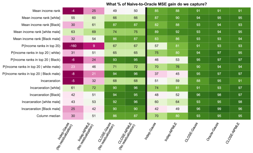
Notes.

Each column is an empirical Bayes strategy that we consider, and each row is a different definition of $\vartheta_{i}$. The table shows relative performance, defined as the squared error improvement over naive, normalized as a percentage of the improvement of oracle over naive. That is, if we think of going to oracle from naive as the total extent of risk gains via empirical Bayes methods, this relative performance denotes how much of those gains each method captures. The last row shows the column median. Since we rely on Monte Carlo approximations of oracle, the resulting Monte Carlo error causes close-npmle to outperform oracle in the top right. Results are averaged over 1,000 Monte Carlo draws.

For absolute, un-normalized performance of independent-gauss, independent-npmle, close-npmle, and oracle, see Figure B.10. ∎

Figure 4. Table of relative squared error Bayes risk for various empirical Bayes approaches

Figure 4 plots the main results from this calibrated simulation. For each method and each target variable, we display a relative measure of gain in terms of mean-squared error. For each method, we calculate its squared error gain over naive, as a percentage of the squared error gain of oracle over naive. If we think of the oracle-naive difference as the total size of the “statistical pie,” then Figure 4 shows how much of this pie each method captures. A value of 70 in Figure 4, for instance, indicates that a particular method captures 70% of the possible extent of risk gains for a particular parameter definition.

The first four columns show the relative mean-squared error performance without residualizing against covariates. That is, empirical Bayes shrinkage is directly on $(\tilde{Y}_{i},\sigma_{i})$ without access to the covariate information. We see that methods which assume prior independence—independent-gauss and independent-npmle—perform worse than methods based on close. Across the 15 variables, the median proportion of possible gains captured by independent-gauss is only 30%. This value is 51% for independent-npmle, and 87% for close-npmle. Individually for each variable, among the first four columns, close-npmle uniformly dominates all three other methods. This is because the standard error $\sigma_{i}$ contains much of the predictive power of the covariates, and using that information can be very helpful when the researcher does not have rich covariate information.

The next five columns show performance when the methods do have access to covariate information. Compared to their no-covariates counterparts, the methods that assume prior independence do substantially better, since the covariates absorb some dependence between $\vartheta_{i}$ and $\sigma_{i}$. For mean rank, after covariate residualization, there appears to be little dependence between $\theta_{i}$ and $\sigma_{i}$. independent-npmle and close-npmle perform similarly, capturing almost all of the available gains. Both methods slightly outperform the Gaussian methods for mean rank.

For the other two outcome variables, top-20 probability and incarceration, the dependence between $\theta_{i}$ and $\sigma_{i}$ is stronger, and close-based methods display substantial improvements over independent-gauss and independent-npmle. close-npmle achieves near-oracle performance across the different definitions of $\theta_{i}$ (capturing a median of 95% of the oracle-naive gap), and uniformly dominates all other feasible methods.

So far, we have tested the methods in a synthetic environment set up to imitate the real data. Next, we turn to an empirical application that uses the coupled bootstrap (Section 4.3) estimator of performance.

5.3. Validation exercise via coupled bootstrap

Our second empirical exercise uses the coupled bootstrap described in Section 4.3 for the ranking policy problem in Bergman et al. (2023). Throughout, we choose $\omega$ to emulate a 90-10 train-test split on the micro-data.

Bergman et al. (2023) use empirical Bayes methods to select the top third Census tracts in Seattle, based on economic mobility—which we view as a top-$m$ selection problem (Decision Problem 3). Can close-npmle make better selections—can it select tracts with higher $\vartheta_{i}$ on average? Specifically, we imagine scaling up Bergman et al. (2023)’s exercise and perform independent-gauss and close-npmle for all Census tracts in the largest twenty Commuting Zones. We then select the top third of tracts within each Commuting Zone, according to empirical Bayesian posterior means for $\vartheta_{i}$. Additionally, to faithfully mimic Bergman et al. (2023), here we perform all empirical Bayes procedures within Commuting Zone. That is, for each of the twenty Commuting Zones that we consider, we execute all empirical Bayes methods—including the residualization by covariates—with only $\tilde{Y}_{i},\sigma_{i}$ of tracts within the Commuting Zone.

(a) Estimated performance difference relative to naive

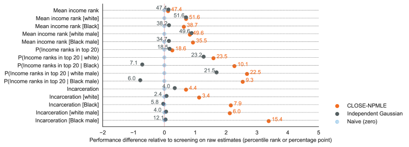
(b) Estimated performance difference relative to picking uniformly at random

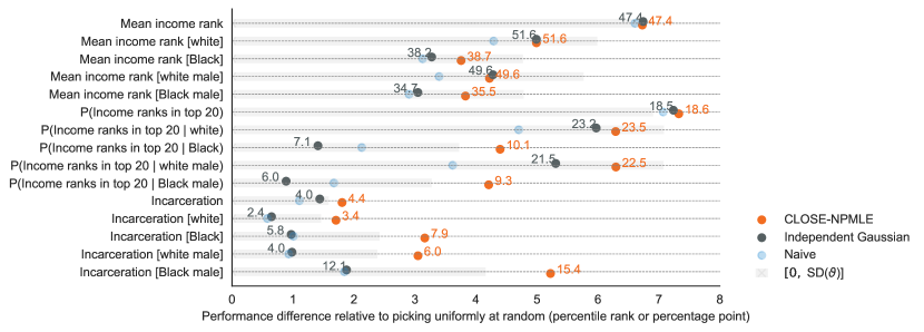
Notes.

These figures show the estimated performance of various decision rules over 1,000 draws of coupled bootstrap. Empirical Bayes methods, including residualization with respect to the covariates, are applied within each Commuting Zone. Performance is measured as the mean $\vartheta_{i}$ among selected Census tracts. All decision rules select the top third of Census tracts within each Commuting Zone. Figure (a) plots the estimated performance gap relative to naive, where we annotate with the estimated performance for close-npmle and independent-gauss. Figure (b) plots the estimated performance gap relative to picking uniformly at random; we continue to annotate with the estimated performance. The shaded regions in Figure (b) have lengths equal to the unconditional standard deviation of the underlying parameter $\vartheta$. ∎

Figure 5. Performance of decision rules in top-$m$ selection exercise

Figure 5(a) shows the estimated performance gap between a given empirical Bayes method and naive as the $x$-position of the dots. The estimated performance, defined as the average $\vartheta_{i}$ among those selected (3), of each method is shown in the annotated figures. According to these estimates, close-npmle generally improves over independent-gauss.

For the mean rank variables, using close-npmle generates substantial gains for mobility measures for Black individuals (0.8 percentile ranks for Black men and 0.5 percentile ranks for Black individuals). To put these gains in dollar terms, the Housing Choice Voucher holders in Bergman et al. (2023) have incomes around $19,000, and for these individuals, an incremental percentile rank amounts to about $1,000. Thus, the estimated gain in terms of mean income rank is roughly $500–800. For the other two outcomes, top-20 probability and incarceration, the gains are even more sizable, especially for Black individuals. These gains are as high as 2–3 percentage points on average in terms of these two variables.

Bergman et al. (2023) select tracts based on mean rank pooled. For this measure, there is little additional gain from using close-npmle, at least when residualized against sufficiently rich covariates. Nevertheless, since about half of the trial participants are Black in bergman2019creating setting, one might consider providing more personalized recommendations by targeting measures of economic mobility for finer demographic subgroups. If we select tracts based on these demographic-specific measures of economic mobility, close-npmle then provides economically significant improvements.

We can think of the performance gap between independent-gauss and naive as the value of basic empirical Bayes. If practitioners find using the standard empirical Bayes method to be a worthwhile investment over screening on the raw estimates directly, perhaps they reveal that the value of basic empirical Bayes is economically significant. Across the 15 measures, the improvement of close-npmle over independent-gauss is on median 320% of the value of basic empirical Bayes, where the median is attained by mean rank for Black individuals. Thus, the additional gain of close-npmle over independent-gauss is substantial compared to the value of basic empirical Bayes. If the latter is economically significant, then it is similarly worthwhile to use close-npmle instead.

For 3 of the 15 measures, including our running example, independent-gauss in fact underperforms naive, rendering the estimated value of basic empirical Bayes negative. As a result, we consider a different normalization in Figure 5(b). Figure 5(b) plots the difference between a given method’s performance and the estimated mean $\vartheta_{i}$ for a given measure. Analogous to the value of basic empirical Bayes, we think of the difference between independent-gauss’s performance and the estimated mean $\vartheta_{i}$ as the value of data, since choosing the tracts randomly in the absence of data has expected performance equal to mean $\vartheta_{i}$. If the mobility estimates are at all useful for decision-making, the value of data must be economically significant.

Across the 15 measures considered, the gain of close-npmle is on median 25% of the value of data. For six of the 15 measures, the gain of close-npmle exceeds the value of data. For mean rank for Black individuals, the incremental value of close-npmle over independent-gauss is about 15% of the value of data, which is already sizable. These relative gains are more substantial for the binarized outcome variables top-20 probability and incarceration. For our running example (top-20 probability for Black individuals), this incremental gain of close-npmle is 210% the value of data. That is, relative to choosing randomly, close-npmle delivers gains 3.1 times that of independent-gauss.

6. Conclusion

This paper studies empirical Bayes methods in the heteroskedastic Gaussian location model. We argue that prior independence—the assumption that the precision of estimates does not predict the true parameter—is theoretically questionable and often empirically rejected. Empirical Bayes shrinkage methods that rely on prior independence can generate worse posterior mean estimates, and screening decisions based on these estimates can suffer as a result. They may even be worse than the selection decisions made with the raw estimates directly.

Instead of treating $\theta_{i}$ as independent from $\sigma_{i}$, we model its conditional distribution as a location-scale family. This assumption leads naturally to a family of empirical Bayes strategies that we call close. We prove that close-npmle attains minimax-optimal rates in Bayes regret, extending previous theoretical results. That is, it approximates infeasible oracle Bayes posterior means as competently as statistically possible. Our main theoretical results are in terms of squared error, which we further connect to ranking-type decision problems in Bergman et al. (2023). Additionally, we show that an idealized version of close-npmle is robust, with finite worst-case Bayes risk. Lastly, we introduce a simple validation procedure based on coupled bootstrap (Oliveira et al., 2021) and highlight its utility for practitioners choosing among empirical Bayes shrinkage methods.

Simulation and validation exercises demonstrate that close-npmle generates sizable gains relative to the standard parametric empirical Bayes shrinkage method. Across calibrated simulations, close-npmle attains close-to-oracle mean-squared error performance. In a hypothetical, scaled-up version of Bergman et al. (2023), across a wide range of economic mobility measures, close-npmle consistently selects more mobile tracts than does the standard empirical Bayes method. The gains in the average economic mobility among selected tracts, relative to the standard empirical Bayes procedure, are often comparable to—or even multiples of—the value of basic empirical Bayes. These gains are even comparable to the benefit of using standard empirical Bayes procedures over ignoring the data.

We close by highlighting some future directions. In Section 5, we use kernel smoothing methods to estimate the unknown conditional moments $\eta_{0}=(m_{0},s_{0})$. These methods presume a given level of smoothness and do not adapt to the true smoothness of $\eta_{0}$. We can imagine replacing the conditional moment estimation with adaptive methods (e.g., van der Vaart and van Zanten, 2009). With cross-fitting, the regret result should similarly adapt to the $\lVert\cdot\rVert_{\infty}$ rate of the estimators. Additionally, for the purpose of frequentist inference, the procedure of Armstrong et al. (2022) apply in our setting as well and provide confidence sets for the vector of parameters $\theta_{1:n}$ with average coverage guarantees. For frequentist inference on the oracle posterior mean $\mathbb{E}_{P_{0}}[\theta_{i}\mid Y_{i},\sigma_{i}]$, we conjecture that a version of ignatiadis2022confidence procedure—which so far only applies in the homoskedastic Gaussian case—is valid under the location-scale model (2.4).

0Contents   

Part I Proofs and discussions of results except the regret upper bound

Appendix A Proofs and discussions of results except the regret upper bound

A.1. A simple regret rate lower bound: proof of Theorem 2

In this section, we prove Theorem 2, restated below. See 2

Proof.

We consider a specific choice of $G_{0},\sigma_{1:n},$ and $s_{0}$. Namely, suppose $G_{0}\sim\mathcal{N}(0,1)$, $\sigma_{1:n}$ are equally spaced in $[\sigma_{\ell},\sigma_{u}]$, and $s_{0}(\sigma)=(s_{\ell}+s_{u})/2\equiv s_{0}$ is constant. Note that we can represent

$$Y_{i}=\underbrace{\theta_{i}+\sigma_{\ell}W_{i}}_{V_{i}}+(\sigma_{i}^{2}-\sigma_{\ell})^{1/2}U_{i}.$$

for independent Gaussians $W_{i},U_{i}\sim\mathcal{N}(0,1)$. Suppose we are additionally given $V_{i},\sigma_{\ell}$. The expanded class of estimators $\tilde{\theta}_{1:n}$ that may depend on $V_{i},\sigma_{\ell}$ is larger than the estimators $\hat{\theta}_{1:n}$. Moreover, since $((V_{i},\sigma_{i})_{i=1}^{n},\sigma_{\ell})$ is sufficient for $\theta_{1:n}$, we may restrict attention to $\tilde{\theta}_{1:n}$ that depend solely on $V_{1:n},\sigma_{1:n},\sigma_{\ell}$.

Under our assumptions, the oracle posterior means $\theta_{i}^{*}$ are equal to

$$\theta_{i}^{*}=\frac{s_{0}^{2}}{s_{0}^{2}+\sigma_{i}^{2}}Y_{i}+\frac{\sigma_{i}^{2}}{s_{0}^{2}+\sigma_{i}^{2}}m_{0}(\sigma_{i})$$

For a given vector of estimates $\tilde{\theta}_{1:n}$, we can form

$$\hat{m}(\sigma_{i})=\frac{s_{0}^{2}+\sigma_{i}^{2}}{\sigma_{i}^{2}}\left({\tilde{\theta}_{i}-\frac{s_{0}^{2}}{s_{0}^{2}+\sigma_{i}^{2}}Y_{i}}\right)$$

Then

$$\mathbb{E}\left[{\frac{1}{n}\sum_{i=1}^{n}(\tilde{\theta}_{i}-\theta_{i}^{*})^{2}}\right]=\mathbb{E}\left[{\frac{1}{n}\sum_{i=1}^{n}\left({\frac{\sigma_{i}^{2}}{s_{0}^{2}+\sigma_{i}^{2}}}\right)^{2}(\hat{m}(\sigma_{i})-m_{0}(\sigma_{i}))^{2}}\right]\gtrsim\mathbb{E}\left[{\frac{1}{n}\sum_{i=1}^{n}(\hat{m}(\sigma_{i})-m_{0}(\sigma_{i}))^{2}}\right].$$

We have just shown that

$$\inf_{\hat{\theta}_{1:n}}\sup_{\sigma_{1:n},P_{0}}\mathbb{E}\left[{\frac{1}{n}\sum_{i=1}^{n}(\hat{\theta}_{i}-\theta_{i})^{2}-(\theta_{i}^{*}-\theta_{i})^{2}}\right]\gtrsim\inf_{\hat{m}}\sup_{m_{0}}\mathbb{E}\left[{\frac{1}{n}\sum_{i=1}^{n}(\hat{m}(\sigma_{i})-m_{0}(\sigma_{i}))^{2}}\right]$$

where the supremum is over $m_{0}$ satisfying Assumption 4, and the infimum is over all randomized estimators of $m_{0}(\sigma_{1}),\ldots,m_{0}(\sigma_{n})$ with data $(V_{i},\sigma_{i})$. Note that the squared error loss on the right-hand side takes expectation over the fixed design points $\sigma_{1},\ldots,\sigma_{n}$.

Lastly, we connect the squared loss on the design points to the $L_{2}$ loss of estimating $m_{0}(\cdot)$ with homoskedastic data $V_{i}\sim\mathcal{N}(m_{0}(\sigma_{i}),\sigma_{\ell}^{2}+s_{0}^{2})$. Since we are simply confronted with a nonparametric regression problem, note that we may translate and rescale so that the design points $\sigma_{1:n}$ are equally spaced in $[0,1]$ and the variance of $V_{i}$ is 1—potentially changing the constant $A_{1}$ for the Hölder smoothness condition. The remaining task is to connect the average $\ell_{2}$ loss on a set of equally spaced grid points to the $L_{2}$ loss over the interval.

Observe that for any $\hat{m}(\sigma_{1}),\ldots,\hat{m}(\sigma_{n})$, there is a function $\tilde{m}:[0,1]\to\mathbb{R}$ such that its average value on $[1+(i-1)/n,1+i/n]$ is $\hat{m}(\sigma_{i})$:

$$n\int_{[1+(i-1)/n,1+i/n]}\tilde{m}(\sigma)\,d\sigma=\hat{m}(\sigma_{i}).$$

Now, note that

$$\int_{0}^{1}(\tilde{m}(x)-m_{0}(x))^{2}\,dx =\sum_{i=1}^{n}\int_{[(i-1)/n,i/n]}(\tilde{m}(x)-m_{0}(x))^{2}\,dx$$

$$\leq 2\sum_{i=1}^{n}\int_{[(i-1)/n,i/n]}(\tilde{m}(x)-m_{0}(\sigma_{i}))^{2}+(m_{0}(\sigma_{i})-m_{0}(x))^{2}\,dx$$ (Triangle inequality)

$$\leq 2\sum_{i=1}^{n}\left[{\frac{1}{n}(\hat{m}_{i}-m_{0}(\sigma_{i}))^{2}+\frac{L^{2}}{n^{3}}}\right]$$

$$=\frac{2}{n}\sum_{i=1}^{n}(\hat{m}_{i}-m_{0}(\sigma_{i}))^{2}+\frac{2L^{2}}{n^{2}}.$$

The third line follows by observing (i) $\int_{I}(\tilde{m}(x)-m_{0}(\sigma_{i}))^{2}\,dx=\left({n\int_{I}\tilde{m}(x)\,dx-m_{0}(\sigma_{i})}\right)^{2}\frac{1}{n}$ and (ii) $m_{0}(\cdot)$ is Lipschitz for some constant $L$ since $p\geq 1$ in Assumption 4.

Therefore,

$$\inf_{\hat{m}}\sup_{m_{0}}\mathbb{E}\left[{\frac{1}{n}\sum_{i=1}^{n}(\hat{m}(\sigma_{i})-m_{0}(\sigma_{i}))^{2}}\right]\geq\frac{1}{2}\inf_{\tilde{m}}\sup_{m_{0}}\left\{{\mathbb{E}\left[{\int_{0}^{1}(\tilde{m}(x)-m_{0}(x))^{2}\,dx}\right]-\frac{2L^{2}}{n^{2}}}\right\}\gtrsim_{\mathcal{H}}n^{-\frac{2p}{2p+1}},$$

where the last inequality follows from the well-known result of $L_{2}$ minimax regression rate for Hölder classes. See, for instance, Corollary 2.3 in Tsybakov (2008). ∎

Remark A.1.

For ease of interpretation, Theorem 2 is stated in the expected regret version, which is slightly disconnected from the upper bound Theorem 1, which conditions on a high-probability event. Observe that Theorem 1 immediately implies the in-probability upper bound on $\mathrm{MSERegret}_{n}$:

$$\mathrm{MSERegret}_{n}(\hat{G}_{n},\hat{\eta})=O_{P}\left({n^{-\frac{2p}{2p+1}}(\log n)^{\frac{2+\alpha}{\alpha}+3+2\beta_{0}}}\right).$$

Using the in-probability version of the minimax lower bound for nonparametric regression in Theorem 2 then implies an analogous lower bound (See, for instance, Theorems 2.4 and 2.5 in Tsybakov, 2008). $\blacksquare$

A.2. Relating other decision objects to squared-error loss

See 3

Proof.

1. We compute

   $$\mathrm{UMRegret}_{n} =\frac{1}{n}\sum_{i=1}^{n}\mathbbm{1}(\theta_{i}^{*}\geq c_{i})(\theta_{i}-c_{i})-\frac{1}{n}\sum_{i=1}^{n}\mathbbm{1}(\hat{\theta}_{i}\geq c_{i})(\theta_{i}-c_{i})$$

   $$=\frac{1}{n}\sum_{i=1}^{n}\left\{{\mathbbm{1}(\theta_{i}^{*}\geq c_{i})-\mathbbm{1}(\hat{\theta}_{i}\geq c_{i})}\right\}(\theta_{i}-c_{i})$$

   By law of iterated expectations, since $\hat{\theta}_{i},\theta_{i}^{*}$ are both measurable with respect to the data,

   $$\mathbb{E}[\mathrm{UMRegret}_{n}] =\mathbb{E}\left[{\frac{1}{n}\sum_{i=1}^{n}\left\{{\mathbbm{1}(\theta_{i}^{*}\geq c_{i})-\mathbbm{1}(\hat{\theta}_{i}\geq c_{i})}\right\}(\theta_{i}^{*}-c_{i})}\right]$$

   Note that, for $\mathbbm{1}(\theta_{i}^{*}\geq c_{i})-\mathbbm{1}(\hat{\theta}_{i}\geq c_{i})$ to be nonzero, $c_{i}$ is between $\hat{\theta}_{i}$ and $\theta_{i}^{*}$. Hence, $|\theta_{i}^{*}-c_{i}|\leq|\theta_{i}^{*}-\theta_{i}|$ and thus

   $$\mathbb{E}[\mathrm{UMRegret}_{n}]\leq\mathbb{E}\left[{\frac{1}{n}\sum_{i=1}^{n}|\theta_{i}^{*}-\theta_{i}|}\right]\leq\mathbb{E}\left[{\frac{1}{n}\sum_{i=1}^{n}(\theta_{i}^{*}-\theta_{i})^{2}}\right]^{1/2}.$$

2. Let $\mathcal{J}^{*}$ collect the indices of the top-$m$ entries of $\theta_{i}^{*}$ and let $\hat{\mathcal{J}}$ collect the indices of the top-$m$ entries of $\hat{\theta}_{i}$. Then,

   $$\frac{m}{n}\mathrm{TopRegret}_{n}^{(m)} =\frac{1}{n}\sum_{i=1}^{n}\left\{{\mathbbm{1}(i\in\mathcal{J}^{*})-\mathbbm{1}(i\in\hat{\mathcal{J}})}\right\}\theta_{i}$$

   and hence, by law of iterated expectations,

   $$\frac{m}{n}\mathbb{E}[\mathrm{TopRegret}_{n}^{(m)}]=\frac{1}{n}\sum_{i=1}^{n}\mathbb{E}\left[{\left\{{\mathbbm{1}(i\in\mathcal{J}^{*})-\mathbbm{1}(i\in\hat{\mathcal{J}})}\right\}\theta_{i}^{*}}\right].$$

   Observe that this can be controlled by applying A.1, where $w_{i}=0$ for all $i\leq n-m$ and $w_{i}=1$ for all $i>n-m$. In this case, $\lVert w\rVert=\sqrt{m}$. Hence,

   $$\frac{m}{n}\mathbb{E}[\mathrm{TopRegret}_{n}^{(m)}]\leq 2\sqrt{\frac{m}{n}}\mathbb{E}\left[{\left({\frac{1}{n}\sum_{i=1}^{n}(\hat{\theta}_{i}-\theta^{*}_{i})^{2}}\right)^{1/2}}\right]\leq 2\sqrt{\frac{m}{n}}\left({\mathbb{E}\left[{\frac{1}{n}\sum_{i=1}^{n}(\hat{\theta}_{i}-\theta^{*}_{i})^{2}}\right]}\right)^{1/2}.$$

   Divide through by $m/n$ to obtain the result.

∎

Proposition A.1.

Suppose $\sigma(\cdot)$ is a permutation such that $\hat{\theta}_{\sigma(n)}\geq\cdots\geq\hat{\theta}_{\sigma(1)}$. Then

$$\frac{1}{n}\sum_{i=1}^{n}w_{i}\theta^{*}_{(i)}-\frac{1}{n}\sum_{i=1}^{n}w_{i}\theta^{*}_{\sigma(i)}\leq\frac{2\lVert w\rVert}{\sqrt{n}}\sqrt{\frac{1}{n}\sum_{i=1}^{n}(\hat{\theta}_{i}-\theta^{*}_{i})^{2}},$$

where $\lVert w\rVert=\sqrt{\sum_{i}w_{i}^{2}}$.

Proof.

We compute

$$\frac{1}{n}\sum_{i=1}^{n}w_{i}\theta^{*}_{(i)}-\frac{1}{n}\sum_{i=1}^{n}w_{i}\theta^{*}_{\sigma(i)} \leq\left|\frac{1}{n}\sum_{i=1}^{n}w_{i}\theta_{(i)}^{*}-\frac{1}{n}\sum_{i=1}^{n}w_{i}\hat{\theta}_{\sigma(i)}\right|+\left|\frac{1}{n}\sum_{i=1}^{n}w_{i}(\hat{\theta}_{\sigma(i)}-\theta^{*}_{\sigma(i)})\right|$$

$$\leq\frac{\lVert w\rVert_{2}}{\sqrt{n}}\cdot\left({\frac{1}{n}\sum_{i=1}^{n}(\theta_{(i)}^{*}-\hat{\theta}_{\sigma(i)})^{2}}\right)^{1/2}+\frac{\lVert w\rVert_{2}}{\sqrt{n}}\sqrt{\frac{1}{n}\sum_{i=1}^{n}(\hat{\theta}_{i}-\theta^{*}_{i})^{2}}$$

$$\leq 2\frac{\lVert w\rVert_{2}}{\sqrt{n}}\sqrt{\frac{1}{n}\sum_{i=1}^{n}(\hat{\theta}_{i}-\theta^{*}_{i})^{2}}.$$

The last step follows from the observation that

$$\sum_{i=1}^{n}(\theta_{(i)}^{*}-\hat{\theta}_{\sigma(i)})^{2}\leq\sum_{i=1}^{n}(\hat{\theta}_{i}-\theta^{*}_{i})^{2}.$$

The left-hand side is the sorted difference between $\theta_{i}^{*}$ and $\hat{\theta}_{i}$. This is smaller than the unsorted difference by an application of the rearrangement inequality. ∎

A.3. Worst-case risk

See 2

Proof.

Note that

$$\hat{\theta}_{i,G_{0}^{*},\eta_{0}}=s_{0}(\sigma_{i})\hat{\tau}_{i,G_{0}^{*},\eta_{0}}+m_{0}(\sigma_{i})$$

and

$$\theta_{i}=s_{0}(\sigma_{i})\tau_{i}+m_{0}(\sigma_{i}).$$

Thus,

$$\frac{1}{n}\sum_{i=1}^{n}(\hat{\theta}_{i}-\theta_{i})^{2}=\frac{1}{n}\sum_{i=1}^{n}s_{0}^{2}(\sigma_{i})(\hat{\tau}_{i,G_{0}^{*},\eta_{0}}-\tau_{i})^{2}.$$

Taking the expected value with respect to $P_{0}\in\mathcal{P}(m_{0},s_{0})$ and apply the bound $\overline{R}_{\mathrm{B}}$, we have that

$$\mathbb{E}\left[{\frac{1}{n}\sum_{i=1}^{n}(\hat{\theta}_{i}-\theta_{i})^{2}}\right]\leq\overline{R}_{\mathrm{B}}\frac{1}{n}\sum_{i=1}^{n}s_{0}^{2}(\sigma_{i}).$$

For the second part, simply observe that the minimum Bayes risk when $P_{0}$ obeys

$$\theta_{i}\mid\sigma_{i}\sim\mathcal{N}(m_{0}(\sigma_{i}),s_{0}^{2}(\sigma_{i}))$$

is

$$\frac{1}{n}\sum_{i=1}^{n}\frac{\sigma_{i}^{2}}{\sigma_{i}^{2}+s_{0}^{2}(\sigma_{i})}s_{0}^{2}(\sigma_{i}),$$

achieved by the oracle version of close-gauss. Thus, when $P_{0}$ is conditionally Gaussian, the Bayes risk of $\hat{\theta}_{i}$ exceeds this quantity. ∎

A.4. Unbiased loss estimation

See 1

Proof.

These are straightforward calculations of the expectation. Since every expectation and variance is conditional on $\theta_{1:n},Y^{(1)}_{1:n},\sigma_{1:n,(1)},\sigma_{1:n,(2)}$, we write $\mathbb{E}[\cdot\mid\mathcal{F}]$ and $\operatorname{Var}(\cdot\mid\mathcal{F})$ without ambiguity.

1. (Decision Problem 1) The unbiased estimation follows directly from the calculation

   $$\mathbb{E}\left[{(Y_{i}^{(2)}-\delta_{i}(Y_{1:n}^{(1)}))^{2}\mid\mathcal{F}}\right]=(\theta_{i}^{(2)}-\delta_{i}(Y_{1:n}^{(1)}))^{2}+\sigma_{i,(2)}^{2}$$

   The conditional variance statement holds by definition.

2. (Decision Problem 2) The unbiased estimation follows directly from the calculation

   $$\mathbb{E}\left[{\delta_{i}(Y_{1:n}^{(1)})(Y_{i}^{(2)}-c_{i})\mid\mathcal{F}}\right]=\delta_{i}(Y_{1:n}^{(1)})(\theta_{i}-c_{i}).$$

   The conditional variance statement follows from

   $$\operatorname{Var}\left[{\delta_{i}(Y_{1:n}^{(1)})(Y_{i}^{(2)}-c_{i})\mid\mathcal{F}}\right]=\delta_{i}(Y_{1:n}^{(1)})\sigma_{1:n,(2)}^{2}.$$

3. (Decision Problem 3) The loss function for Decision Problem 3 is the same as that for Decision Problem 2 with $c_{i}=0$. Since we condition on $Y_{1:n}^{(1)}$, the argument is thus analogous.

∎

A.5. A discrete choice model

There are $n$ options facing $N$ consumers, where each consumer chooses one option. Each option is characterized by idiosyncratic quality $\beta_{j}$ and inherent quality $\alpha_{j}$. The latent quality of an option is $\theta_{j}=\alpha_{j}+\rho\frac{N_{j}}{\mathbb{E}[N]}$, where $N_{j}\leq N$ is the number of consumers using option $j$, generated in equilibrium from a discrete choice model. The term $\rho N_{j}$ reflects externalities generated by the users of an option (congestion). We assume that $\alpha_{j},\beta_{j}\overset{\mathrm{i.i.d.}}{\sim}F$ where $\mu$ denotes $\mathbb{E}[\alpha_{j}+\beta_{j}]$ and $\sigma^{2}_{\alpha},\sigma^{2}_{\beta},\sigma_{\alpha\beta}$ denotes the variances and covariance of $\alpha$ and $\beta$.

To connect this model to our setting, we can imagine that the data analyst has estimates $Y_{j}$ for $\theta_{j}$, whose standard errors are a function of $N_{j}$. The discrete choice model specifies how $N_{j}$ selects on the quality component $\alpha_{j}$, and $\rho$ determines how $\theta_{j}$ is affected by $N_{j}$. We characterize $\operatorname{Cov}(\theta_{j},N_{j})$ as a function of the primitives $\rho,\mu,\sigma_{\alpha},\sigma_{\beta},\sigma_{\alpha\beta}.$

Each individual $i$ is endowed with a private type $\epsilon_{i}=(\epsilon_{i1},\ldots,\epsilon_{iJ})$ of i.i.d Type-1 extreme value random utilities. This prior for $\epsilon_{i}$ is common knowledge and well-specified. $\alpha_{1:n},\beta_{1:n},N$ are common knowledge as well. Each individual $i$ is an expected utility maximizer, where the utility of item $j$ is

$$V_{j}=\left({\alpha_{j}+\beta_{j}+\rho\frac{N_{j,-i}}{N-1}}\right)\exp\left({\epsilon_{ij}}\right)$$

where $N_{j,-i}$ is the number of other individuals choosing item $j$. Since individuals other than $i$ are symmetric to $i$, the expected utility (conditional on what $i$ observes) is

$$\mathbb{E}_{i}V_{j}=(\alpha_{j}+\beta_{j}+\rho\pi_{-ij})\exp\left({\epsilon_{ij}}\right),$$

where $\pi_{-ij}$ is $i$’s prior expectation of $N_{j,-i}/(N-1)$. A Bayes-Nash equilibrium is one in which individual $i$ chooses the option with the highest $\mathbb{E}_{i}V_{j}$ and his beliefs about other individuals, $\pi_{-ij}$, are correct.

Since individuals are ex-ante symmetric, we assume that

$$\pi_{-ij}=\pi_{j}=\operatorname{P}(\mathbb{E}_{i}V_{j}\geq\mathbb{E}_{i}V_{k}\quad\forall k).$$

In such a symmetric equilibrium, $\pi$ solves the system of equations

$$\frac{\alpha_{j}+\beta_{j}+\rho\pi_{j}(N-1)}{\sum_{j}\alpha_{j}+\beta_{j}+\rho\pi_{j}(N-1)}=\pi_{j}\implies\pi_{j}=\frac{\alpha_{j}+\beta_{j}}{\sum_{j}\alpha_{j}+\beta_{j}}.$$

Finally, we assume that the total number of consumers is ex ante random

$$N\mid(\alpha_{1:n},\beta_{1:n})\sim\operatorname{Pois}\left({\lambda\cdot\left({\sum_{j=1}^{n}\alpha_{j}+\beta_{j}}\right)}\right).$$

Assume that the data-generating process draws $\alpha,\beta,N$, and individuals play the Bayes–Nash equilibrium under symmetric beliefs $\pi$. By the thinning property of Poisson processes, we have that

Lemma A.1.

$N_{j}\mid(\alpha_{1:n},\beta_{1:n})\sim\operatorname{Pois}\left({\lambda(\alpha_{j}+\beta_{j})}\right)$ independently across $j$.

Now, under this process, we can compute the covariance between the latent quality $\theta_{j}$ and the sample size $N_{j}$ in closed form:

$$\operatorname{Cov}\left({\theta_{j},N_{j}}\right) =\underbrace{\operatorname{Cov}(\alpha_{j},N_{j})}_{\text{selection}}+\underbrace{\frac{\rho}{\lambda n\mu}\operatorname{Var}(N_{j})}_{\text{congestion}}$$

$$=\lambda(\sigma_{\alpha}^{2}+\sigma_{\alpha\beta})+\frac{\rho}{\lambda n\mu}\left[{\lambda\mu+\lambda^{2}(\sigma^{2}_{\alpha}+\sigma^{2}_{\beta}+2\sigma_{\alpha\beta})}\right]$$

This is positive—meaning that the latent quality is positively associated with precision—iff

$$\frac{\rho}{\lambda n\mu}>-\frac{\operatorname{Cov}(\alpha_{j},N_{j})}{\operatorname{Var}(N_{j})}=-\frac{\sigma_{\alpha}^{2}+\sigma_{\alpha\beta}}{\mu+\lambda(\sigma_{\alpha}^{2}+\sigma_{\beta}^{2}+2\sigma_{\alpha\beta})}.$$

When the selection effect is positive ($\operatorname{Cov}(\alpha_{j},N_{j})$), the above display requires the externality $\rho$ to not be too negative so as to dominate the selection effect. Note that the sign of the selection contribution depends on the covariance between $\alpha$ and $\beta$, and thus could be negative. Moreover, if $\alpha$ instead were an undesirable trait to consumers, then the selection effect may also be negative. The congestion effect similarly does not have to be negative. We allow for positive spillovers by $\rho>0$.

We can interpret various empirical observations through this model:

• For hospital value-added (Chandra et al., 2016), $N_{j}$ positively selects on hospital quality $\alpha_{j}$. This is likely true for most value-added settings.

• For teacher value-added, it is possible (Lazear, 2001; Barrett and Toma, 2013; Mehta, 2019) that teachers may prefer smaller classes, and school administrators may reward good teachers by letting them teach smaller classes. In the lends of this model, $N_{j}$ negatively selects on quality.

• In integenerational mobility, $N_{j}$ is the number of poor minority households. Higher $N_{j}$ leads to oppressive institutions and residential segregation. We can interpret these pernicious effects as a negative $\rho$.

However, this model does not capture all channels through which $\theta_{j}$ can be correlated with $\sigma_{j}$. For instance, the following is difficult to map to the discrete choice model.

• In unbalanced panel data settings, the length of the observed period for a unit—which relates to the precision of the unit’s estimated fixed effect—may be correlated with the underlying fixed effect. This observation dates at least to Olley and Pakes (1996), who note that in a firm panel, those firms with shorter observed period are probably less productive and have to shut down sooner. For value-added modeling of nursing homes, Einav et al. (2022) note that patients with shorter stays at nursing homes typically experience an adverse health event, including death. Such events are presumably more likely for worse nursing homes, again inducing a correlation between nursing home qualities and the sample sizes used to estimate them. Similarly, for teacher value-added, Bruhn et al. (2022) find that teachers who have shorter observed spells in administrative datasets tend to be worse and have noisier value added estimates.

A.6. Interpretation of empirical Bayes sampling model

When the empirical Bayes sampling model fails to hold, empirical Bayes methods do not precisely mimic an oracle Bayesian’s decision. However, in many cases, we can still interpret the empirical Bayes decision rules. In most such cases, the interpretation is in terms of emulating an oracle Bayesian who is constrained. The oracles are constrained either by removing its access to certain information or by restricting its decisions to a particular class. We will consider two scenarios when such an interpration is natural.

A.6.1. Interpretation when independence of units fails

We consider the interpretation of the sampling model (2) when it is misspecified. Recall that we assume $(Y_{i},\theta_{i},\sigma_{i})$ are sampled independently across $i$, with $Y_{i}\mid\theta_{i},\sigma_{i}\sim\mathcal{N}(\theta_{i},\sigma_{i})$. This sampling model can fail in two ways. First, it is possible that $Y_{1:n}\mid\theta_{1:n},\sigma_{1:n}$ are correlated but still multivariate Gaussian. Second, it is possible that $(\theta_{i},\sigma_{i})$ are correlated across $i$. Here, we limit our discussion to Decision Problem 1.

Let $\bm{Y}=(Y_{1},\ldots,Y_{n})$ and $\bm{\theta}=(\theta_{1},\ldots,\theta_{n})^{\prime}$. Let us assume instead that

$$\bm{Y}\mid\bm{\theta},\Sigma\sim\mathcal{N}(\bm{\theta},\Sigma)$$

where $\operatorname{diag}(\Sigma)=[\sigma_{1}^{2},\ldots,\sigma_{n}^{2}]$ and the variance-covariance matrix $\Sigma$ is known. Let $Q_{0}$ be the joint distribution of $\bm{\theta}\mid\Sigma$. Now, the oracle Bayesian—who knows $Q_{0}$—would use $\mathbb{E}_{Q_{0}}[\theta_{i}\mid\bm{Y},\Sigma]$ as their decision rule. The empirical Bayesian can similarly emulate that oracle Bayes decision rule by estimating $Q_{0}$. If the empirical Bayesian is willing to assume that the location-scale assumption (2.4) describes $Q_{0}$:

$$(\theta_{i}\mid\Sigma)\sim(\theta_{i}\mid\sigma_{1:n})\sim G_{0}\left({\frac{\cdot-m_{0}(\sigma_{i})}{s_{0}(\sigma_{i})}}\right),$$

then the empirical Bayesian can similarly implement close, and output estimates of $\mathbb{E}_{Q_{0}}[\theta_{i}\mid\bm{Y},\Sigma]$. We should caveat that the npmle step no longer maximizes the full likelihood of $\bm{Y}$ with respect to $G_{0}$, but a quasi-likelihood that averages over the log-likelihood of each $Y_{i}$ separately, ignoring their joint distribution.

Now, let us consider what interpretation our method has when we erroneously assume either the independence of $Y_{i}$ across $i$ or that $\bm{\theta}_{i}\mid\Sigma$ are independent across $i$. The latter independence may fail, for instance, when the populations index places, and the $\theta_{i}$’s are thought to be spatially correlated (e.g., in Müller and Watson, 2022). Consider the class of separable decision rules, where the forecast for $\theta_{i}$ can depend solely on $Y_{i},\sigma_{i}$:

$$\delta_{i}(\bm{Y},\sigma_{1:n})=\delta_{i}(Y_{i},\sigma_{i}).$$

Consider a constrained oracle Bayesian who is forced to use a separable decision rule. They would use $\mathbb{E}_{Q_{0}}[\theta_{i}\mid Y_{i},\sigma_{i}]$. Note that this constrained decision rule depends on $Q_{0}$ only through the distribution $\theta_{i}\mid\sigma_{i}$ (and not $\theta_{i}\mid\Sigma$). Thus, under the location-scale assumption

$$(\theta_{i}\mid\sigma_{1:n})\sim G_{0}\left({\frac{\cdot-m_{0}(\sigma_{i})}{s_{0}(\sigma_{i})}}\right),$$

close-based methods emulate this oracle Bayesian constrained to separable decision rules. Of course, the resulting empirical Bayesian decision rule is not separable (since $\hat{G}_{n}$ presumably depends on all the data), but it seeks to emulate the best possible separable rule. This interpretation in terms of emulating a constrained oracle Bayesian holds regardless of the joint distribution of $\bm{Y}$ or of $\bm{\theta}$, so long as our specification of the marginal distribution holds. Of course, our regret results do not immediately carry over to this setting.

A.6.2. Interpretation with additional covariates $X_{i}$

Additionally, we may also have population-level covariates $X_{i}$. Let us maintain that $X_{i}$ does not predict the noise in $Y_{i}$:

$$Y_{i}\indep X_{i}\mid\theta_{i},\sigma_{i}.$$

Here, we will discuss two questions. First, how do we handle covariates? Second, what is the difference between using $X_{i}$ and $\sigma_{i}$—is the standard error simply a covariate?

On the first question, there are two ways of incorporating covariates, under similar but distinct assumptions. First, close-methods can be extended to incorporate covariates by augmenting (2.4) to incorporate covariates. That is, we can instead assume that

$$P_{0}(\theta_{i}\leq t\mid X_{i},\sigma_{i})\sim G_{0}\left({\frac{t-m_{0}(\sigma_{i},X_{i})}{s_{0}(\sigma_{i},X_{i})}}\right)$$

and estimate $m_{0},s_{0}$ nonparametrically. Instead of being one-dimensional nonparametric regression problem, they are now $(d+1)$-dimensional nonparametric problems. Under the same Hölder-type smoothness conditions, the corresponding regret rate replaces $n^{-\frac{2p}{2p+1}}$ with $n^{-\frac{2p}{2p+1+d}}$. Second, as we do in the empirical exercises, one could consider a strategy of residualizing against $X_{i}$ in some arbitrary way, performing empirical Bayes, and undoing the residualization. This strategy dates back to Fay and Herriot (1979). That is, with raw data $\tilde{Y}_{i}$ for parameter $\vartheta_{i}$, we can consider forming the residuals $Y_{i}=\tilde{Y}_{i}-b(X_{i})$ and $\theta_{i}=Y_{i}-b(X_{i})$, and perform empirical Bayes methods on $(Y_{i},\theta_{i},\sigma_{i})$. At a high level, we can rationalize this strategy as mimicking a constrained oracle Bayesian who solely has access to $Y_{i},\sigma_{i}$, who knows the joint distribution of $(\theta_{i},\sigma_{i})$, but who does not have access to $X_{i}$. Note that this interpretation is coherent regardless of the transformation $b(X_{i})$, allowing us to be more blasé about modeling $X_{i}$ than the previous approach. In particular, choosing $b(X_{i})=0$ ignores the covariate entirely; the resulting empirical Bayes procedure mimics an oracle that does not have access to $X_{i}$. Of course, when we impose the location-scale assumption (2.4) on $(\theta_{i},\sigma_{i})$, different $b(X_{i})$ gives rise to different—and possibly mutually exclusive—underlying models on $(\vartheta_{i},\sigma_{i},X_{i})$.

On the second question, in an operational sense, $\sigma_{i}$ is simply another covariate. $\sigma_{i}$ is not particularly special in the assumption (A.6.2), and one interpretation of close is treating $\sigma_{i}$ precisely as a covariate to be regressed out. However, $\sigma_{i}$ does occupy a special place in the statistical structure of the problem. The likelihood of the data, $Y_{i}\mid\theta_{i},\sigma_{i}$, depends on $\sigma_{i}$ but not $X_{i}$. This special role of $\sigma_{i}$ means that we must treat it with more care so that the resulting procedure has a coherent interpretation. If we wanted to ignore covariates $X_{i}$, we can imagine an oracle Bayesian who does not have access to $X_{i}$, and the resulting empirical procedure simply mimics that constrained oracle. This line of reasoning does not work with $\sigma_{i}$, since any oracle Bayesian—constrained or otherwise—must have access to $\sigma_{i}$. As a result, we cannot avoid the problem of modeling $\theta_{i}\mid\sigma_{i}$ as easily as we could have avoided modeling $\theta_{i}\mid X_{i},\sigma_{i}$ by changing the goalpost.

A.7. Alternatives to close

A.7.1. Alternative methods

Let us turn to a few specific alternative methods that consider failure of prior independence. We argue that they do not provide a free-lunch improvement over our assumptions. At a glance, these alternative methods have properties summarized in Table 2.

Table 2. Properties of alternative methods

	$t$-ratios	Var. stab. transforms	Random $\hat{\sigma}_{i}$	SURE
Restrict to a class of procedures	✗			✗
Change the loss function	✗	✗
Require access to micro-data			✗
Assume $\theta_{i}$ is independent from some other known nuisance parameter, e.g. $n_{i}$		✗	✗
Parametric restrictions on the micro-data		✗	✗

Alternative 1 (Working with $t$-ratios).

We may consider normalizing $\sigma_{i}$ away by working with $t$-ratios $T_{i}\equiv\frac{Y_{i}}{\sigma_{i}}\mid(\sigma_{i},\theta_{i})\sim\mathcal{N}\left({\theta_{i}/\sigma_{i},1}\right).$ The resulting problem is homoskedastic by construction. It is natural to consider performing empirical Bayes shrinkage assuming that $\frac{\theta_{i}}{\sigma_{i}}\overset{\mathrm{i.i.d.}}{\sim}H_{0}$, and use, say, $\sigma_{i}\mathbf{E}_{\hat{H}_{n}}\left[{\frac{\theta_{i}}{\sigma_{i}}\mid T_{i}}\right]$ as an estimator for the posterior mean of $\theta_{i}$ (Jiang and Zhang, 2010). However, such an approach approximates the optimal decision rule within a restricted class on a different objective.

Let us restrict decision rules to those of the form $\delta_{i,\text{t-stat}}(Y_{i},\sigma_{i})=\sigma_{i}h(Y_{i}/\sigma_{i})$. The oracle Bayes choice of $h$ is $h^{\star}(T_{i})=\frac{\mathbb{E}\left[{\sigma_{i}\theta_{i}\mid T_{i}}\right]}{\mathbb{E}[\sigma_{i}^{2}\mid T_{i}]}$. However, $h^{\star}$ is not the posterior mean of $\theta_{i}/\sigma_{i}$ given the $t$-ratio $T_{i}$, unless $\sigma_{i}^{2}\indep\theta_{i}/\sigma_{i}$. On the other hand, the loss function that does rationalize the posterior mean $h(T_{i})=\mathbb{E}[\theta_{i}/\sigma_{i}\mid T_{i}]$ is the precision-weighted compound loss $L(\bm{\delta},\theta_{1:n})=\frac{1}{n}\sum_{i=1}^{n}\sigma_{i}^{-2}(\delta_{i}-\theta_{i})^{2}$. Thus, rescaling posterior means on $t$-ratios achieves optimality for a weighted objective among a restricted class of decision rules $\delta_{i,\text{t-stat}}$. $\blacksquare$

Alternative 2 (Variance-stabilizing transforms).

Second, we may consider a variance-stabilizing transform when the underlying micro-data are Bernoulli and $\theta_{i}$ is a Bernoulli mean (Efron and Morris, 1975; Brown, 2008). Specifically, we rely on the asymptotic approximation

$$\sqrt{n_{i}}(Y_{i}-\theta_{i})\underset{n_{i}\to\infty}{\overset{d}{\longrightarrow}}\mathcal{N}(0,\theta_{i}(1-\theta_{i})).$$

A variance-stabilizing transform can disentangle the dependence: Let $W_{i}=2\arcsin(\sqrt{Y_{i}})$ and $\omega_{i}=2\arcsin(\sqrt{\theta_{i}})$, and, by the delta method,

$$\sqrt{n_{i}}\left({W_{i}-\omega_{i}}\right)\underset{n_{i}\to\infty}{\overset{d}{\longrightarrow}}\mathcal{N}(0,1).\quad\text{ Thus, approximately, }W_{i}\mid\omega_{i},n_{i}\sim\mathcal{N}\left({\omega_{i},\frac{1}{n_{i}}}\right).$$

One might consider an empirical Bayes approach on the resulting $W_{i}$. Note that $W_{i}$ may still violate prior independence, since $\omega_{i}$ may not be independent of $n_{i}$. Moreover, squared error loss on estimating $\omega_{i}=2\arcsin(\sqrt{\theta_{i}})$ is different from squared error loss on estimating $\theta_{i}$. We do not know of any guarantees for the loss function on $\theta_{i}$, $\frac{1}{n}\sum_{i=1}^{n}(\delta_{i}-\sin^{2}(\omega_{i}/2))^{2}$, when we perform empirical Bayes analysis on $\omega_{i}$. $\blacksquare$

Alternative 3 (Treating the standard error as estimated).

Lastly, if the researcher has access to micro-data, Gu and Koenker (2017) and Fu et al. (2020) propose empirical Bayes strategies that treat $\sigma_{i}$ as noisy as well, in which we know the likelihood of $(Y_{i},\sigma_{i})$. This approach allows for dependence between $\theta_{i}$ and $\sigma_{i}$ but assumes independence between $(\theta_{i},\sigma_{i})$ and some other known nuisance parameter. To describe their model, we introduce more notation. Let $Y_{ij},j=1,\ldots,n_{i},$ denote the micro-data for population $i$, where, for each $i$, we are interested in the mean of $Y_{ij}$. Let $Y_{i}$ denote their sample mean and $S_{i}^{2}$ denote their sample variance, where $\sigma_{i}^{2}=S_{i}^{2}/n_{i}$. Let $\sigma_{i0}^{2}$ denote the true variance of observations from population $i$.

Both papers work under Gaussian assumptions on the micro-data. This parametric assumption on the micro-data—which is stronger than we require—implies that $Y_{i}\indep S_{i}^{2}\mid(\sigma_{i0},\theta_{i},n_{i})$ with marginal distributions:

$$Y_{i}\mid\sigma_{i0},\theta_{i},n_{i}\sim\mathcal{N}\left({\theta_{i},\frac{\sigma_{i0}^{2}}{n_{i}}}\right)\qquad S_{i}^{2}\mid\sigma_{i0},\theta_{i},n_{i}\sim\operatorname{Gamma}\left({\frac{n_{i}-1}{2},\frac{1}{2\sigma_{i0}^{2}}}\right).$$

They then propose empirical Bayes methods treating $\mathbf{Y}_{i}\equiv(Y_{i},S_{i}^{2})$ as noisy estimates for parameters $\bm{\theta}_{i}\equiv(\theta_{i},\sigma_{i0}^{2})$. This formulation allows $\bm{\theta}_{i}$ to have a flexible distribution, and thus allows for dependence between $\theta_{i}$ and $\sigma_{i0}^{2}$. However, since the known sample size $n_{i}$ enters the likelihood of $\mathbf{Y}_{i}$, this approach still assumes that $n_{i}\indep\bm{\theta}_{i}$. $\blacksquare$

This discussion is not to say that close is necessarily preferable to these alternatives. It highlights that the possible dependence between $\theta_{i}$ and $\sigma_{i}$ cannot be easily resolved. As summarized in Table 2, existing alternatives compromise on optimality, use a different loss function, or implicitly assume $\theta_{i}$ is independent from components of $\sigma_{i}^{2}$ (e.g., $n_{i}$). Of course, depending on the empirical context, these may well be reasonable features.

In contrast, our approach models $\theta_{i}\mid\sigma_{i}$ directly via the location-scale assumption (2.4). A natural question is whether other types of modeling may be superior—which we turn to next. We argue that the location-scale model uniquely capitalizes on the appealing properties of the npmle-based empirical Bayes approaches.

A.7.2. Alternative models for $\theta_{i}\mid\sigma_{i}$

One alternative is simply treating the joint distribution of $(\theta_{i},\sigma_{i})$ fully nonparametrically. For instance, an $f$-modeling approach with Tweedie’s formula implies that an estimate of the conditional distribution $Y_{i}\mid\sigma_{i}$ is all one needs for computing the posterior means (Brown and Greenshtein, 2009; Liu et al., 2020). However, conditional density estimation is a challenging problem, and most available methods do not exploit the restriction that $Y_{i}\mid\sigma_{i}$ is a Gaussian convolution. Similarly, one could consider flexible parametric $g$-modeling of $\theta_{i}\mid\sigma_{i}$ in the vein of the log-spline sieve of Efron (2016). This has the advantage of estimating a smooth prior at the cost of having tuning parameters. We are not aware of regret results for this approach.

If we commit to making some substantive restriction on the joint distribution of $(\theta_{i},\sigma_{i})$, it is fair to ask why the conditional location-scale restriction (2.4) is necessarily preferable. However, if we wish to capitalize on the theoretical and computational advantages of npmle, it is natural to consider a class of procedures that transform the data in some way and use the npmle on the resulting transformed data to estimate the prior distribution (Section A.7.3 gives a heuristic justification for this strategy). If we wish to preserve the Gaussian location model structure on the transformed data, then effectively we can only consider affine transformations (i.e., $Z=a(\sigma)+b(\sigma)Y$) (shown in Lemma A.2 below). If we further wish that $Z$ obeys a Gaussian location model in which prior independence holds (i.e., $\tau\equiv a(\sigma)+b(\sigma)\theta$ is independent from $\nu\equiv b(\sigma)\sigma$)—so that we can apply npmle-based approaches assuming prior independence—then we have no other choice but to assume (2.4). Thus, the conditional location-scale assumption is uniquely well-suited to capitalize on the favorable properties of npmle already established in the literature, which we extend via Theorem 1.

Lemma A.2.

Let $Y\sim\mathcal{N}(\theta,\sigma^{2})$ with known $\sigma^{2}$. Consider a strictly increasing and differentiable function $g(\cdot)$. Let $Z=h(Y)$. Then the corresponding family of distributions of $Z$ is a natural exponential family if and only if $h(Y)=a+bY$.

Proof.

The “if” part ($\Longleftarrow$) is immediate. We focus on the “only if” ($\implies$) part. Writing the distribution of $Y$ as an exponential family,

$$p_{Y}(y)\propto\exp\left({y\frac{\theta}{\sigma^{2}}+g(y,\sigma)+A(\theta,\sigma)}\right)$$

for some $g(y,\sigma)$ and $A(\theta,\sigma)$. Note that we have

$$p_{Z}(z)=p_{Y}(y)\bigg{\lvert}\frac{dy}{dz}\bigg{\rvert}=p_{Y}(h^{-1}(z))\frac{dh^{-1}(z)}{dz}$$

Thus, writing in exponential family form, for some $\tilde{g}$, we have that

$$p_{Z}(z)\propto\exp\left({h^{-1}(z)\frac{\theta}{\sigma^{2}}+\tilde{g}(z,\sigma)+A(\theta,\sigma)}\right)$$

Suppose $Z$ follows a natural exponential family with natural parameter $q(\theta;\sigma)$. Then we can write

$$h^{-1}(z)\frac{\theta}{\sigma^{2}}=zq(\theta;\sigma)+v(\theta,\sigma)+w(z).$$

Since $h$ is strictly monotone and differentiable, so is $h^{-1}$. Taking the $z$-derivative of both sides:

$$\frac{dh^{-1}}{dz}=\frac{\sigma^{2}}{\theta}q(\theta;\sigma)+w^{\prime}(z)\frac{\sigma^{2}}{\theta}.$$

Since the left-hand side does not depend on $\theta$, it follows that

$$\frac{q(\theta;\sigma)+w^{\prime}(z)}{\theta}$$

is free of $\theta$ for all $z$. Suppose $w^{\prime}(z)$ is not constant, then for $z_{1}\neq z_{2}$ and $w^{\prime}(z_{1})\neq w^{\prime}(z_{2})$, the difference is $\theta$-dependent

$$\frac{q(\theta;\sigma)+w^{\prime}(z_{1})}{\theta}-\frac{q(\theta;\sigma)+w^{\prime}(z_{2})}{\theta}=\frac{w^{\prime}(z_{1})-w^{\prime}(z_{2})}{\theta}.$$

Hence $w^{\prime}(z)$ is a constant. As a result, $\frac{dh^{-1}}{dz}$ does not depend on $z$, and hence $h(z)=a+bz$. ∎

A.7.3. Model-free interpretation of close-npmle

When the location-scale model fails to hold, it remains sensible to consider estimating the npmle on an affine transformation of the data, as in close-npmle.

Let us first consider a given affine transformation of the data—not necessarily $\tau=\frac{Z-m_{0}(\sigma)}{s_{0}(\sigma)}$—into $(Z_{i},\tau_{i},\nu_{i})$ for which $\tau_{i}\mid\nu_{i}\sim H_{(i)}$, and ask why npmle is reasonable. In population, npmle seeks to minimize the average Kullback–Leibler (KL) divergence between the distribution of the estimates $Z_{i}$ and the distribution implied by the convolution $H\star\mathcal{N}(0,\nu_{i}^{2})$:

$$\max_{H}\frac{1}{n}\sum_{i=1}^{n}\mathbb{E}_{Z_{i}\sim f_{H_{(i)},\nu_{i}}}\left[{\log f_{H,\nu_{i}}(Z_{i})}\right]\text{, equivalent to }\min_{H}\,\frac{1}{n}\sum_{i=1}^{n}\operatorname{KL}\left({f_{H_{(i)},\nu_{i}}\,\|\,f_{H,\nu_{i}}}\right),$$

where $f_{H,\nu}$ is the density of the convolution $H\star\mathcal{N}(0,\nu^{2})$. As shown by Jiang and Zhang (2009) and Jiang (2020) (see Section C.3), the regret in mean-squared error under a misspecified prior $\tau_{i}\sim H$ is upper bounded by the average squared Hellinger distance between the distribution of the data and the distribution implied by $H$. The average Hellinger distance is further upper bounded by the average KL divergence:

$$\frac{1}{n}\sum_{i=1}^{n}h^{2}\left({f_{H_{(i)},\nu_{i}},f_{H,\nu_{i}}}\right)\leq\frac{1}{n}\sum_{i=1}^{n}\operatorname{KL}\left({f_{H_{(i)},\nu_{i}}\,\|\,f_{H,\nu_{i}}}\right).$$

In this sense, even under misspecification ($H_{(i)}\neq H_{(j)}$), npmle chooses a common distribution $H$ that minimizes an upper bound of regret.

Now that we have a justification for the npmle, let us consider the transformation we would like to choose. It is reasonable, then, to choose the affine transform $(a(\sigma),b(\sigma))$ so that the resulting conditional distributions $H_{(i)}$ of the transformed parameter $\tau_{i}\mid\sigma_{i}$ are similar—under some distance measure. Doing so does not recover prior independence on the transformed data but limits the extent of non-independence. Choosing $a(\sigma),b(\sigma)$ to ensure that $\tau_{i}\mid\sigma_{i}$ has the same first two moments is intuitively reasonable, and actually has a formal interpretation in terms of information-theoretic divergences and optimal transport metrics, at least in a large-$\sigma$ regime (Chen and Niles-Weed, 2022).

Part II Additional empirical results

Appendix B Additional empirical exercises

B.1. Positivity of $s_{0}(\cdot)$ in the Opportunity Atlas data

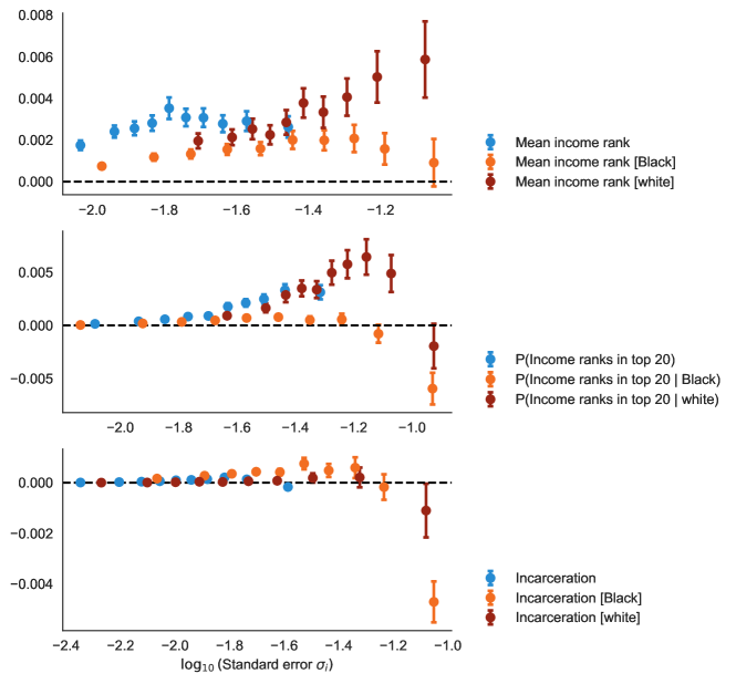
Figure B.1. Estimated conditional variance $s_{0}^{2}(\sigma)$, binned into deciles, with 95% uniform confidence intervals shown.

In the Opportunity Atlas data, we often observe that the estimated conditional variance is negative: $\hat{s}_{0}^{2}<0$. To test if this is due to sampling variation or underdispersion of the Opportunity Atlas estimates relative to the estimated standard error, we consider the following upward-biased estimator of $s_{0}^{2}(\sigma_{i})$. Without loss, let us sort the $Y_{i},\sigma_{i}$ by $\sigma_{i}$, where $\sigma_{1}\leq\cdots\leq\sigma_{n}$. Let $S_{i}=\frac{1}{2}\left[{(Y_{i+1}-Y_{i})^{2}-(\sigma_{i}^{2}+\sigma_{i+1}^{2})}\right]$. Note that

$$\mathbb{E}[S_{i}\mid\sigma_{1:n}]=\frac{1}{2}\mathbb{E}[(\theta_{i+1}-\theta_{i})^{2}\mid\sigma_{1:n}]=\frac{s_{0}^{2}(\sigma_{i+1})+s_{0}^{2}(\sigma_{i})}{2}+\frac{1}{2}(m_{0}(\sigma_{i+1})-m_{0}(\sigma_{i}))^{2}\geq\frac{s_{0}^{2}(\sigma_{i+1})+s_{0}^{2}(\sigma_{i})}{2}.$$

Hence $S_{i}$ is an overestimate of the successive averages of $s_{0}(\sigma)$. Figure B.1 plot the estimated conditional expectation of $S_{i}$ given $\sigma_{i}$, using a sample of $(S_{1},S_{3},S_{5},\ldots)$ so that the $S_{i}$’s used are mutually independent. We see that for many measures of economic mobility, we can reject $\mathbb{E}[S_{i}\mid\sigma_{i}]\geq 0$, indicating some overdispersion in the data.

B.2. Robustness checks for the calibration exercise in Section 5

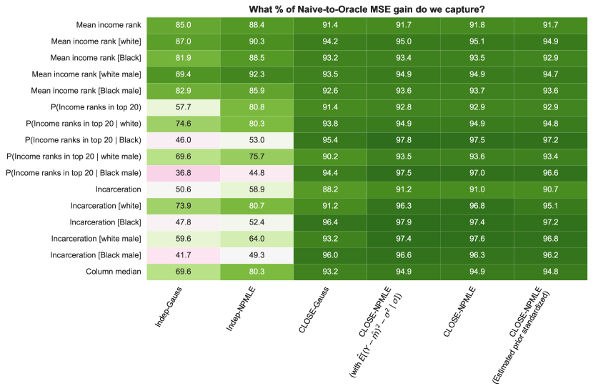
Figure B.2. Additional close-npmle variants for the calibrated simulation in Section 5. Here the results average over 100 replications.

In Figure B.2, we evaluate two variants of close-npmle. The first variant (column 4) uses an estimator for $s_{0}(\cdot)$ that smoothes the difference $(Y-\hat{m}(\sigma))^{2}-\sigma^{2}$, rather than smoothing $(Y-\hat{m}(\sigma))^{2}$ and then subtracting $\sigma^{2}$. Since local linear regression suffers from bias coming from the convexity of the underlying unknown function, smoothing the difference can perform better, as the convexity bias differences out. The second variant (column 6) projects the estimated npmle $\hat{G}_{n}$ to the space of mean zero and variance one distributions, by normalizing by its estimated first and second moments. Neither variant performs appreciably differently from the main version of close-npmle (column 5) that we demonstrate in the main text.

B.3. Simulation exercise setup

This section describes the details of the simulation exercise in Section 5. We restrict to the 10,109 tracts within the twenty largest Commuting Zones. Tracts with missing information are dropped for each measure of mobility. Specifically, the simulated data-generating process is as follows:

1. Residualize $\tilde{Y}_{i}$ against some covariates $X_{i}$ to obtain $\beta$ and residuals $Y_{i}$. Estimate the conditional moments $m_{0},s_{0}$ on $(Y_{i},\sigma_{i})$ via local linear regression, described in Appendix G.

2. Partition $\sigma$ into vingtiles. Within each vingtile $j$, estimate an npmle $G_{j}$ over the data $\left({\frac{Y_{i}-m_{0}(\sigma_{i})}{s_{0}(\sigma_{i})},\frac{\sigma_{i}}{s_{0}(\sigma_{i})}}\right)$ and normalize $G_{j}$ to have zero mean and unit variance. Sample $\tau_{i}^{*}\mid\sigma_{i}\sim G_{j}$ if observation $i$ falls within vingtile $j$.

3. Let $\vartheta_{i}^{*}=s_{0}(\sigma_{i})\tau_{i}^{*}+m_{0}(\sigma_{i})+\beta^{\prime}X_{i}$ and let $\tilde{Y}_{i}^{*}\mid\theta_{i}^{*},\sigma_{i}\sim\mathcal{N}(\theta_{i}^{*},\sigma_{i}^{2})$.

The estimated $\beta,m_{0},s_{0}$ will serve as the basis for the true data-generating process in the simulation, and as a result we do not denote it with hats.

The covariates used are poverty rate in 2010, share of Black individuals in 2010, mean household income in 2000, log wage growth for high school graduates, mean family income rank of parents, mean family income rank of Black parents, the fraction with college or post-graduate degrees in 2010, and the number of children—and the number of Black children—under 18 living in the given tract with parents whose household income was below the national median. These covariates are included in chetty2018opportunity publicly available data, and these descriptions are from their codebook. This set of covariates is not precisely the same as what is used in Bergman et al. (2023). Bergman et al. (2023) additionally use economic mobility estimates for a later birth cohort, which are not included in the publicly released version of the Opportunity Atlas. The “number of children” variables are used by (Chetty et al., 2020) as a population weighting variable; they contain some information on the implicit micro-data sample sizes $n_{i}$.

B.4. Different Monte Carlo setup

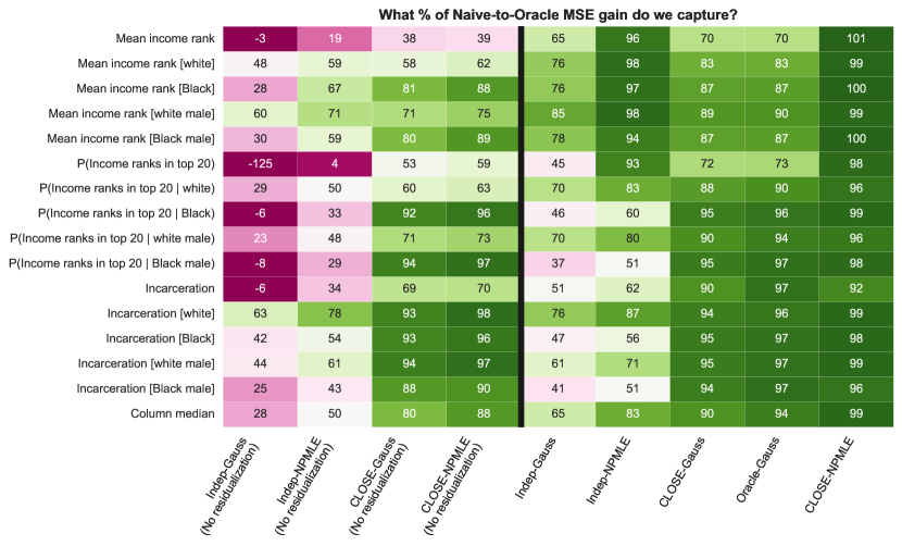
Figure B.3. Analogue of Figure 4 for the data-generating process in Section B.4. Here the results average over 100 replications.

We have also conducted a Monte Carlo exercise where we replace (Sim-2) with the following step:

• For each $\sigma_{i}$, let

  $$\alpha_{i}=\frac{1}{2}+\frac{1}{2}\frac{m_{0}(\sigma_{i})-\min_{i}m_{0}(\sigma_{i})}{\max_{i}m_{0}(\sigma_{i})-\min_{i}(\sigma_{i})}\in[1/2,1]$$

  We sample $\tau_{i}^{*}\mid\sigma_{i}$ as a scaled and shifted $\mathrm{Weibull}$ distribution with shape $\alpha_{i}$. The scaling and translation ensures that $\tau_{i}\mid\sigma_{i}$ has mean zero and variance one. Because we choose the Weibull distribution, the shape parameter $\alpha_{i}$ corresponds exactly to $\alpha$ in Assumption 2. Our choices of $\alpha_{i}$ implies that $\tau_{i}\mid\sigma_{i}$ has thicker tails than exponential and does not have a moment-generating function.

The Weibull distribution has thicker tails and is skewed, and as a result, npmle-based methods tend to greatly outperform methods based on assuming Gaussian priors. Figure B.3 show the analogue of Figure 4 for this data-generating process. Indeed, we see that independent-npmle improves over independent-gauss considerably, and similarly for close-npmle and oracle-gauss.

B.5. MSE in validation exercise with coupled bootstrap

We compare empirical Bayes procedures for the squared error estimation problem (Decision Problem 1), in the setting of the validation exercise in Section 5. Since this is an empirical application on real, rather than synthetic, data, we no longer have access to oracle estimators. As a result, for the relative MSE performance, we normalize by a different benchmark. We can think of the performance gain of independent-gauss over naive as the value of doing basic, standard empirical Bayes shrinkage. We normalize each method’s estimated MSE improvement against naive as a multiple of this “value of basic empirical Bayes.” Figure B.4(a) shows the resulting relative performance. Since our notion of relative performance has changed, we use a different color scheme. A value of $1$ means that a method does exactly as well as independent-gauss, and a value of $2$ means that, relative to naive, a method doubles the gain of basic empirical Bayes. Performance on a non-relative scale is shown in Figure B.4(b).

(a) Normalized performance

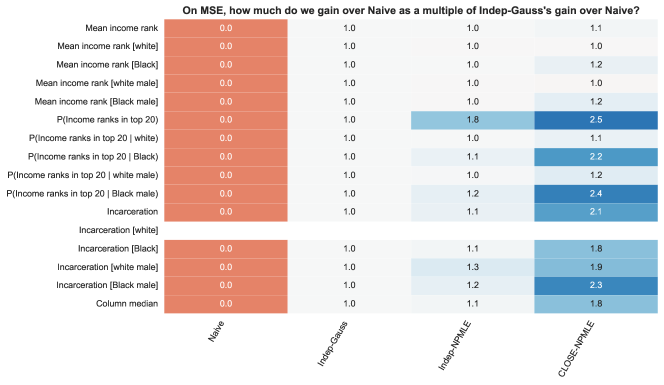
(b) Performance difference against naive

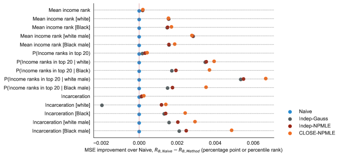
Notes.

In panel (a), each column is an empirical Bayes strategy that we consider, and each row is a different definition of $\theta_{i}$. The table shows relative performance, defined as the squared error improvement over naive, normalized as a multiple of the improvement of independent-gauss over naive. By definition, such a measure is zero for naive and one for independent-gauss. The last row shows the column median. The mean-squared error estimates average over 100 coupled bootstrap draws. For the variable incarceration for white individuals, the strategy independent-gauss underperform naive, and the resulting ratio is thus undefined.

Panel (b) shows the difference in MSE against naive. ∎

Figure B.4. Estimated MSE Bayes risk for various empirical Bayes strategies in the validation exercise.

We find that our empirical patterns from the calibrated simulation Figure 4 mostly persists on real data. In particular, independent-npmle offers small improvements over independent-gauss. Nevertheless, close-npmle continues to dominate other methods. Across the definitions of $\vartheta_{i}$, close-npmle generates a median of 180% the value of basic empirical Bayes. That is, on mean-squared error, moving from independent-gauss to close-npmle is about half as valuable as moving from naive to independent-gauss. For our running example (top-20 probability for Black individuals), moving from independent-gauss to close-npmle is more valuable than moving from naive to independent-gauss. If practitioners find using the standard empirical Bayes method to be a worthwhile investment over using the raw estimates directly, then they may find using close-npmle over independent-gauss to be a similarly worthwhile investment.

B.6. Empirical Bayes pooling over all Commuting Zones in validation exercise

Here, we repeat the exercise in Figure 5, but we now estimate empirical Bayes methods pooling over all Commuting Zones. We still pick the top third of every Commuting Zone. Our first exercise repeats Figure 5 in this setting, shown in Figure B.5. The results are extremely similar.

(a) Estimated performance of close-npmle, independent-gauss, and naive

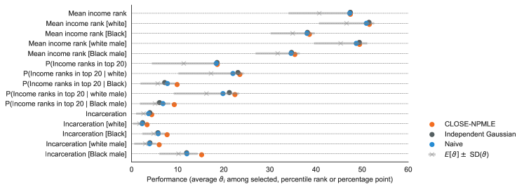
(b) Estimated performance difference relative to naive

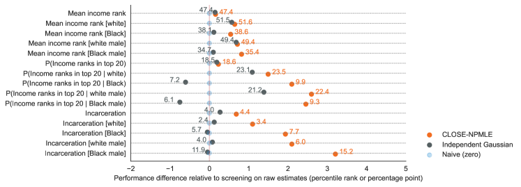
(c) Estimated performance difference relative to picking uniformly at random

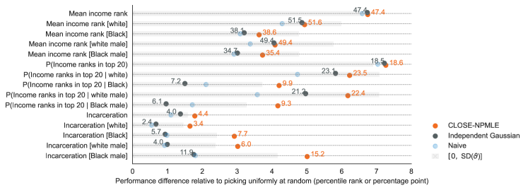
Notes.

These figures show the estimated performance of various decision rules over 100 coupled bootstrap draws. Performance is measured as the mean $\vartheta_{i}$ among selected Census tracts. All decision rules select the top third of Census tracts within each Commuting Zone. Figure (a) plots the estimated performance, averaged over 100 coupled bootstrap draws, with the estimated unconditional mean and standard deviation shown as the grey interval. Figure (b) plots the estimated performance gap relative to naive, where we annotate with the estimated performance for close-npmle and independent-gauss. Figure (c) plots the estimated performance gap relative to picking uniformly at random; we continue to annotate with the estimated performance. The shaded regions in Figure (c) have lengths equal to the unconditional standard deviation of the underlying parameter $\vartheta$. ∎

Figure B.5. Performance of decision rules in top-$m$ selection exercise

Separately, we consider the version of this exercise without covariates in Figure B.6. We see that covariates are extremely important for the performance of independent-gauss, as it frequently underperforms naive without covariates. By comparison, they are less important for the performance of close-npmle, as $\sigma_{i}$ contains a lot of the signal in the tract-level covariates.

(a) Estimated performance of close-npmle, independent-gauss, and naive

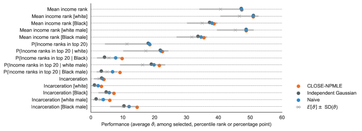
(b) Estimated performance difference relative to naive

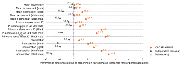
(c) Estimated performance difference relative to picking uniformly at random

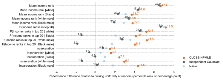
Notes.

These figures show the estimated performance of various decision rules over 100 coupled bootstrap draws. There are no covariates to residualize against. Performance is measured as the mean $\vartheta_{i}$ among selected Census tracts. All decision rules select the top third of Census tracts within each Commuting Zone. Figure (a) plots the estimated performance, averaged over 100 coupled bootstrap draws, with the estimated unconditional mean and standard deviation shown as the grey interval. Figure (b) plots the estimated performance gap relative to naive, where we annotate with the estimated performance for close-npmle and independent-gauss. Figure (c) plots the estimated performance gap relative to picking uniformly at random; we continue to annotate with the estimated performance. The shaded regions in Figure (c) have lengths equal to the unconditional standard deviation of the underlying parameter $\vartheta$. ∎

Figure B.6. Performance of decision rules in top-$m$ selection exercise (No covariates)

B.7. The tradeoff between accurate targeting and estimation precision

In this section, we investigate the tradeoff between accurate targeting and estimation precision. That is, suppose $\theta_{i},Y_{i},\sigma_{i}$ and $\vartheta_{i},\Upsilon_{i},\varsigma_{i}$ are two sets variables corresponding to two measures of economic mobility. For instance, perhaps $\theta_{i}$ is mean rank for Black individuals and $\vartheta_{i}$ is mean rank pooling over all individuals. Suppose the decision maker would like to select populations with high $\theta_{i}$, but the estimates $Y_{i}$ are noisier than the estimates $\Upsilon_{i}$. It is plausible that screening on posterior means for $\vartheta_{i}$ might outperform screening on posterior means for $\theta_{i}$.

We investigate this question via coupled bootstrap in the Bergman et al. (2023) exercise. In particular, we let the subscript $b$ (resp. $w$) denote quantities for Black (resp. white) individuals. We assume that $Y_{ib}\indep Y_{iw}\mid\theta_{ib},\theta_{iw}$. For each tract, we construct $\pi_{i}=n_{ib}/n_{i}$, where $n_{i}$ (resp. $n_{i}$) is the number of (resp. Black) children under 18 living in the given tract with parents whose household income was below the national median. Let $\theta_{i}=\pi_{i}\theta_{ib}+(1-\pi_{i})\theta_{iw}$ be a pooled measure, where

$$Y_{i}=\pi_{i}Y_{ib}+(1-\pi_{i})Y_{iw}\mid\theta_{i}\sim\mathcal{N}(0,\pi_{i}^{2}\sigma_{ib}^{2}+(1-\pi_{i})^{2}\sigma_{iw}^{2}).$$

Each coupled bootstrap draw adds and subtracts noise $Z_{ib},Z_{iw}$ to $Y_{ib}$ and $Y_{iw}$, where $Z_{ib}\indep Z_{iw}$. Bootstrap draws for $Y_{i}$ are constructed by taking the $\pi_{i}$-combination of bootstrap draws for $Y_{ib},Y_{iw}$.

Here, we investigate whether screening tracts based on posterior mean estimates for $\theta_{iw}$ or $\theta_{i}$ generates better decisions in terms of $\theta_{ib}$, owing to the precision in $Y_{iw}$ and $Y_{i}$. Figure B.7 shows estimated performances of different empirical Bayes methods by different proxy variables that the screening targets. For each measure of economic mobility for Black individuals, dots on the thick black dashed line correspond to screening on the corresponding $\theta_{ib}$. Dots on the red (resp. blue) dashed line correspond to screening on $\theta_{iw}$ (resp. $\theta_{i}$). We see that for all three measures of economic mobility, using close-npmle to screen on the original parameter $\theta_{ib}$ performs best. In other words, the benefits of higher precision are insufficient to offset inaccurate targeting.

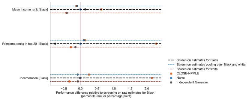
Notes.

Estimated performance for different empirical Bayes methods by different proxy parameters. The performance of screening based on the raw $Y_{ib}$ is normalized to zero. All results are over 100 coupled bootstrap draws. ∎

Figure B.7. Performances of strategies that screen on posterior means for more precisely estimated parameters

(a) Not residualized by covariates

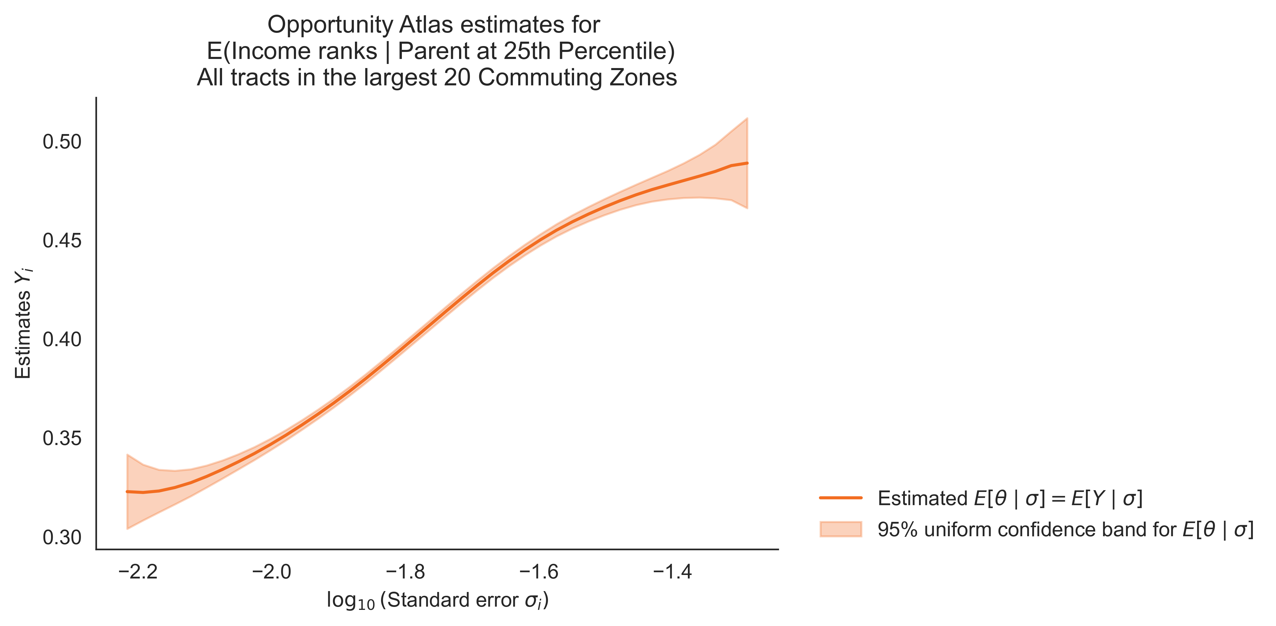
(b) Residualized by covariates

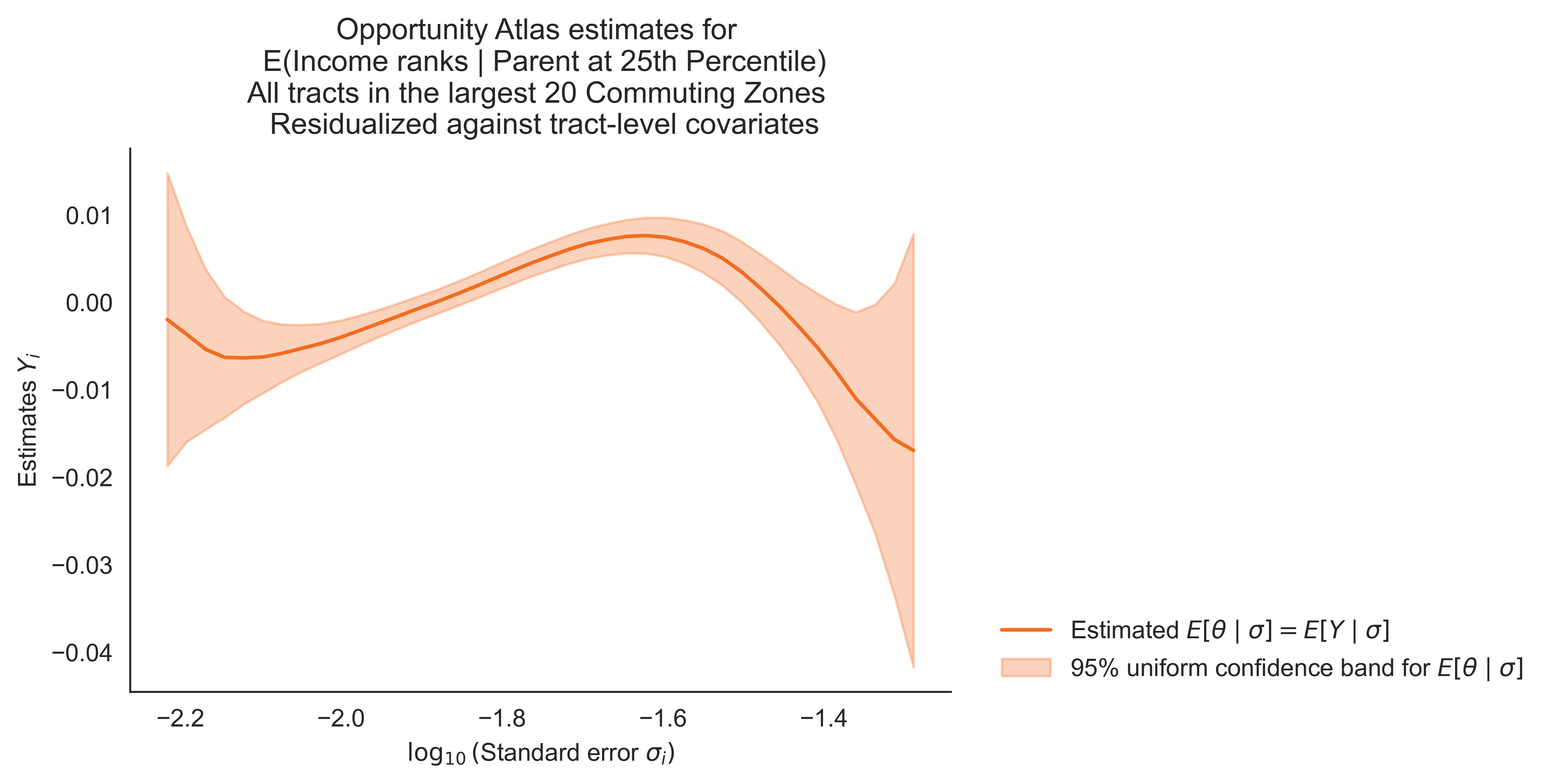
Notes.

This figure shows the estimated $\mathbb{E}[\theta\mid\sigma]$ for mean income rank, pooling over all demographic groups. This is the measure of economic mobility used by Bergman et al. (2023). The estimation and the confidence band procedures are the same as those in Figure 1. In panel (a), $\theta_{i},Y_{i}$ are defined as unresidualized measures of mean income rank. In panel (b), we treat $\theta_{i},Y_{i}$ as residualized against a vector of tract-level covariates as specified in Section B.3. ∎

Figure B.8. Estimated $\mathbb{E}[\theta\mid\sigma]$ for mean income rank among those with parents at the 25^th percentile

Figure B.9. The analogue of Figure 1 where $Y_{i},\theta_{i}$ are treated as residualized against a vector of covariates as specified in Section B.3.

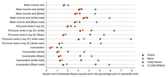
Figure B.10. Absolute mean-squared error risk of key methods for the calibrated simulation in Figure 4

Part III Regret control proofs

Appendix C Setup, assumptions, and notation

We recall some notation in the main text, and introduce additional notation. Recall that we assume $n\geq 7$. We observe $(Y_{i},\sigma_{i})_{i=1}^{n},(Y_{i},\sigma_{i})\in\mathbb{R}\times\mathbb{R}_{>0}$ such that

$$Y_{i}\mid(\theta_{i},\sigma_{i})\sim\mathcal{N}(\theta_{i},\sigma_{i}^{2})$$

and $(Y_{i},\theta_{i},\sigma_{i})$ are mutually independent. Assume that the joint distribution for $(\theta_{i},\sigma_{i})$ takes the location-scale form (2.4)

$$\theta_{i}\mid(\sigma_{1},\ldots,\sigma_{n})\sim G_{0}\left({\frac{\theta_{i}-m_{0}(\sigma_{i})}{s_{0}(\sigma_{i})}}\right)$$

Define shorthands $m_{0i}=m_{0}(\sigma_{i})$ and $s_{0i}=s_{0}(\sigma_{i})$. Define the transformed parameter $\tau_{i}=\frac{\theta_{i}-m_{0i}}{s_{0i}}$, the transformed data $Z_{i}=\frac{Y_{i}-m_{0i}}{s_{0i}}$, and the transformed variance $\nu_{i}^{2}=\frac{\sigma_{i}^{2}}{s_{0i}^{2}}$. By assumption,

$$Z_{i}\mid(\tau_{i},\nu_{i})\sim\mathcal{N}(\tau_{i},\nu_{i}^{2})\quad\tau_{i}\mid\nu_{1},\ldots,\nu_{n}\overset{\mathrm{i.i.d.}}{\sim}G_{0}.$$

Let $\hat{\eta}=(\hat{m},\hat{s})$ denote estimates of $m_{0}$ and $s_{0}$. Likewise, let $\hat{\eta}_{i}=(\hat{m}_{i},\hat{s}_{i})=(\hat{m}(\sigma_{i}),\hat{s}(\sigma_{i}))$. For a given $\hat{\eta}$, define

$$\hat{Z}_{i}=\hat{Z}_{i}(\hat{\eta})=\hat{Z}_{i}(Z_{i},\hat{\eta})=\frac{Y_{i}-\hat{m}_{i}}{\hat{s}_{i}}=\frac{s_{0i}Z_{i}+m_{0i}-\hat{m}_{i}}{\hat{s}_{i}}\quad\hat{\nu}_{i}^{2}=\hat{\nu}_{i}^{2}(\hat{\eta})=\frac{\sigma_{i}^{2}}{\hat{s}_{i}^{2}}.$$

We will condition on $\sigma_{1:n}$ throughout, and hence we treat them as fixed.

For generic $G$ and $\nu>0$, define

$$f_{G,\nu}(z)=\int_{-\infty}^{\infty}\varphi\left({\frac{z-\tau}{\nu}}\right)\frac{1}{\nu}\,G(d\tau).$$

to be the marginal density of some mixed normal deviate $Z\mid\tau\sim\mathcal{N}(\tau,\nu^{2})$ with mixing distribution $\tau\sim G$. As a shorthand, we write

$$f_{i,G}=f_{G,\nu_{i}}(Z_{i})\quad f^{\prime}_{i,G}=f_{G,\nu_{i}}^{\prime}(Z_{i})$$

Let the average squared Hellinger distance be

$$\overline{h}^{2}(f_{G_{1},\bm{\cdot}},f_{G_{2},\bm{\cdot}})=\frac{1}{n}\sum_{i=1}^{n}h^{2}\left({f_{G_{1},\nu_{i}},f_{G_{2},\nu_{i}}}\right).$$

For generic values $\eta=(m,s)$ and distribution $G$, define the log-likelihood function

$$\psi_{i}(z,\eta,G)=\psi_{i}(z,(m,s),G)=\log\int_{-\infty}^{\infty}\varphi\left({\frac{\hat{Z}_{i}(\eta)-\tau}{\hat{\nu}_{i}(\eta)}}\right)\,G(d\tau)=\log\left({\hat{\nu}_{i}(\eta)\cdot f_{G,\hat{\nu}_{i}(\eta)}(\hat{Z}_{i}(\eta))}\right)$$

Define

$$\mathrm{Sub}_{n}(G)=\left({\frac{1}{n}\sum_{i=1}^{n}\psi_{i}(Z_{i},\eta_{0},G)-\frac{1}{n}\sum_{i=1}^{n}\psi_{i}(Z_{i},\eta_{0},G_{0})}\right)_{+}$$

as the log-likelihood suboptimality of $G$ against the true distribution $G_{0}$, evaluated on the true, but unobserved, transformed data $Z_{i},\nu_{i}$.

Fix some generic $G$ and $\eta=(m,s)$. The empirical Bayes posterior mean ignores the fact that $G,\eta$ are potentially estimated. The posterior mean for $\theta_{i}=s_{i}\tau+m_{i}$ is

$$\hat{\theta}_{i,G,\eta}=m_{i}+s_{i}\mathbf{E}_{G,\hat{\nu}_{i}(\eta)}[\tau\mid\hat{Z}_{i}(\eta)].$$

Here, we define $\mathbf{E}_{G,\nu}\left[{h(\tau,Z)\mid z}\right]$ as the function of $z$ that equals the posterior mean for $h(\tau,Z)$ under the data-generating model $\tau\sim G$ and $Z\mid\tau\sim\mathcal{N}(\tau,\nu)$. Explicitly,

$$\mathbf{E}_{G,\nu}\left[{h(\tau,Z)\mid z}\right]=\frac{1}{f_{G,\nu}(z)}\int h(\tau,z)\varphi\left({\frac{z-\tau}{\nu}}\right)\frac{1}{\nu}\,G(d\tau).$$

Explicitly, by Tweedie’s formula,

$$\mathbf{E}_{G,\hat{\nu}_{i}(\eta)}[\tau_{i}\mid\hat{Z}_{i}(\eta)]=\hat{Z}_{i}(\eta)+\hat{\nu}_{i}^{2}(\eta)\frac{f^{\prime}_{G,\hat{\nu}_{i}(\eta)}(\hat{Z}_{i}(\eta))}{f_{G,\hat{\nu}_{i}(\eta)}(\hat{Z}_{i}(\eta))}.$$

Hence, since $\hat{Z}_{i}(\eta)=\frac{Y_{i}-m_{i}}{s_{i}}$,

$$\hat{\theta}_{i,G,\eta}=Y_{i}+s_{i}\hat{\nu}_{i}^{2}(\eta)\frac{f^{\prime}_{G,\hat{\nu}_{i}(\eta)}(\hat{Z}_{i}(\eta))}{f_{G,\hat{\nu}_{i}(\eta)}(\hat{Z}_{i}(\eta))}.$$

Define $\theta_{i}^{*}=\hat{\theta}_{i,G_{0},\eta_{0}}$ to be the oracle Bayesian’s posterior mean. Fix some positive number $\rho>0$, define a regularized posterior mean as

$$\hat{\theta}_{i,G,\eta,\rho}=Y_{i}+s_{i}\hat{\nu}_{i}^{2}(\eta)\frac{f^{\prime}_{G,\hat{\nu}_{i}(\eta)}(\hat{Z}_{i}(\eta))}{f_{G,\hat{\nu}_{i}(\eta)}(\hat{Z}_{i}(\eta))\vee\frac{\rho}{\hat{\nu}_{i}(\eta)}}$$

and define $\theta^{*}_{i,\rho}=\hat{\theta}_{i,G_{0},\eta_{0},\rho}$ correspondingly.

Lastly, we will also define

$$\varphi_{+}(\rho)=\varphi^{-1}(\rho)=\sqrt{\log\frac{1}{2\pi\rho^{2}}}\quad\rho\in(0,(2\pi)^{-1/2})$$ (C.3)

so that $\varphi(\varphi_{+}(\rho))=\rho$. Observe that $\varphi_{+}(\rho)\lesssim\sqrt{\log(1/\rho)}$.

C.1. Assumptions

Recall the assumptions we stated in the main text.

See 1

See 2

See 3

See 4

C.2. Regret control: result statement

Define the regret as the difference between the mean-squared error of some feasible posterior means $\hat{\theta}_{i,G,\eta}$ against the mean-squared error of the oracle posterior means

$$\mathrm{MSERegret}_{n}(G,\eta) =\frac{1}{n}\sum_{i=1}^{n}(\hat{\theta}_{i,G,\eta}-\theta_{i})^{2}-\frac{1}{n}\sum_{i=1}^{n}(\theta^{*}_{i}-\theta_{i})^{2}$$

$$=\frac{1}{n}\sum_{i=1}^{n}(\hat{\theta}_{i,G,\eta}-\theta^{*}_{i})^{2}+\frac{2}{n}\sum_{i=1}^{n}(\theta^{*}_{i}-\theta_{i})(\hat{\theta}_{i,G,\eta}-\theta^{*}_{i})$$ (C.4)

(C.4) decomposes the MSE regret into a mean term that equals the mean-squared distance between the feasible posterior means and the oracle posterior means, as well as a term that is mean zero conditional on the data $Y_{1},\ldots,Y_{n}$, since $\theta_{i}^{*}-\theta_{i}$ represents irreducible noise.

Fix sequences $\Delta_{n}>0$ and $M_{n}>0$. Define the following “good” event which we use in Theorem F.1:

$$A_{n}=\left\{{\lVert\hat{\eta}-\eta\rVert_{\infty}\equiv\max(\lVert\hat{m}-m_{0}\rVert_{\infty},\lVert\hat{s}-s_{0}\rVert_{\infty})\leq\Delta_{n},\,\overline{Z}_{n}\equiv\max_{i\in[n]}(|Z_{i}|\vee 1)\leq M_{n}}\right\}.$$

On the event $A_{n}$, the nuisance estimates $\hat{\eta}$ are good, and the data $Z_{i}$ are not too large. Note that, with $\Delta_{n}=C_{1}n^{-\frac{p}{2p+1}}(\log n)^{\beta_{0}},$

$$A_{n}=\mathbf{A}_{n}(C_{1})\cap\left\{{\overline{Z}_{n}\leq M_{n}}\right\},$$

where $\mathbf{A}_{n}$ is the event in (3.1.2).

Here, we prove the version of our result stated in the main text.

See 1

Proof.

Immediately by Assumption 4(2–3), we can choose $C_{1,\mathcal{H}}$ so that $\operatorname{P}(\mathbf{A}_{n}(C_{1,\mathcal{H}}))\geq 1-\delta$. Let $\Delta_{n}=C_{1,\mathcal{H}}n^{-\frac{p}{2p+1}}(\log n)^{\beta_{0}}$ and $M_{n}=C(\log n)^{1/\alpha}$ for some $C$ to be chosen. Both $C_{1,\mathcal{H}}$ and $C$ may depend on $\delta$. Moreover, we can decompose

$$\mathbb{E}\left[{\mathrm{MSERegret}_{n}(\hat{G}_{n},\hat{\eta})\mid\mathbf{A}_{n}(C_{1,\mathcal{H}})}\right]$$

$$\leq\frac{1}{1-\delta}\left\{{\mathbb{E}\left[{\mathrm{MSERegret}_{n}(\hat{G}_{n},\hat{\eta})\mathbbm{1}(A_{n})}\right]+\mathbb{E}\left[{\mathrm{MSERegret}_{n}(\hat{G}_{n},\hat{\eta})\underbrace{\mathbbm{1}(\mathbf{A}_{n}(C_{1,\mathcal{H}}),\overline{Z}_{n}>M_{n})}_{\mathbf{A}_{n}\setminus A_{n}}}\right]}\right\}$$

$$\lesssim_{\mathcal{H}}n^{-\frac{2p}{2p+1}}(\log n)^{\frac{2+\alpha}{\alpha}+3+2\beta_{0}}+\frac{1}{n}(\log n)^{2/\alpha}$$ (Theorems F.1 and F.1)

$$\lesssim_{\mathcal{H}}n^{-\frac{2p}{2p+1}}(\log n)^{\frac{2+\alpha}{\alpha}+3+2\beta_{0}}$$

Note that the application of Theorems F.1 and F.1 implicitly picks some constant for $M_{n}=C(\log n)^{1/\alpha}$. This concludes the proof. ∎

See 1

Proof.

Let $\Delta_{n},M_{n}$ as in the proof of Theorem 1. Decompose

$$\mathbb{E}[\mathrm{MSERegret}_{n}(\hat{G}_{n},\hat{\eta})] =\mathbb{E}[\mathrm{MSERegret}_{n}(\hat{G}_{n},\hat{\eta})\mathbbm{1}(A_{n})]+\mathbb{E}[\mathrm{MSERegret}_{n}(\hat{G}_{n},\hat{\eta})\mathbbm{1}(A_{n}^{\mathrm{C}})]$$

$$=\mathbb{E}[\mathrm{MSERegret}_{n}(\hat{G}_{n},\hat{\eta})\mathbbm{1}(A_{n})]+\mathbb{E}[\mathrm{MSERegret}_{n}(\hat{G}_{n},\hat{\eta})\mathbbm{1}(\mathbf{A}_{n}^{\mathrm{C}}\cup\left\{{Z_{n}>M_{n}}\right\})]$$

$$\leq\mathbb{E}[\mathrm{MSERegret}_{n}(\hat{G}_{n},\hat{\eta})\mathbbm{1}(A_{n})]+\mathbb{E}[\mathrm{MSERegret}_{n}(\hat{G}_{n},\hat{\eta})\mathbbm{1}(\mathbf{A}_{n}^{\mathrm{C}})]$$

$$\quad+\mathbb{E}[\mathrm{MSERegret}_{n}(\hat{G}_{n},\hat{\eta})\mathbbm{1}(\overline{Z}_{n}>M_{n})]$$

$$\lesssim_{\mathcal{H}}n^{-\frac{2p}{2p+1}}(\log n)^{\frac{2+\alpha}{\alpha}+3+2\beta_{0}}+\frac{2}{n}(\log n)^{2/\alpha}$$ (Theorems F.1 and F.1)

$$\lesssim_{\mathcal{H}}n^{-\frac{2p}{2p+1}}(\log n)^{\frac{2+\alpha}{\alpha}+3+2\beta_{0}},$$

where our application of Lemma F.1 uses the assumption that $\operatorname{P}(\mathbf{A}_{n}(C_{1,\mathcal{H}})^{\mathrm{C}})=\mathbbm{1}(\lVert\hat{\eta}-\eta\rVert_{\infty}>\Delta_{n})\leq\frac{1}{n^{2}}.$ ∎

Remark C.1 (Relaxing Assumption 4(4)).

Note that the event $\mathbf{A}_{n}(C)$ implies $s_{0\ell}/2\leq\hat{s}\leq 2s_{0u}$ for all sufficiently large $n>N_{C,s_{0\ell},s_{0u},p,\beta_{0}}$. Since we condition on $\mathbf{A}_{n}(C)$ in Theorem 1, we can drop Assumption 4(3) by only requiring (1) to hold for all sufficiently large $n$. This is a minor modification since Theorem 1 is an upper bound on the convergence rate. On the other hand, dropping Assumption 4(4) does affect regret control on the event $\mathbf{A}_{n}^{\mathrm{C}}(C_{1})$ below. Our truncation rule for $\hat{s}(\cdot)$ in Appendix G ensures that $\hat{s}(\cdot)\geq\frac{c}{n}$. We show in Appendix G that this is sufficient for the conclusion of 1. $\blacksquare$

C.3. Regret control: proof ideas

We now discuss the main ideas and the structure of our argument. Existing work (Soloff et al., 2021) controls the following quantity, in our notation,

$$\mathbb{E}\left[{\mathrm{MSERegret}_{n}^{\tau}(\hat{G}_{n},\eta_{0})}\right]\equiv\mathbb{E}\left[{\frac{1}{n}\sum_{i=1}^{n}(\hat{\tau}_{i,\hat{G}_{n}^{*},\eta_{0}}-\tau_{i}^{*})^{2}}\right]$$

where $\hat{\tau}_{i,\hat{G}_{n},\eta_{0}}=\mathbf{E}_{\hat{G}_{n},\nu_{i}}[\tau\mid Z_{i}]$ and $\hat{G}_{n}^{*}$ is an approximate NPMLE on the data $(Z_{i},\nu_{i})_{i=1}^{n}$ (Theorem 8 in Soloff et al. (2021)).

They do so by showing that, loosely speaking,

1. For some constant $C$ and rate function $\delta_{n}$, with high probability, the NPMLE achieves low average squared Hellinger distance:

   $$\operatorname{P}\left({\overline{h}^{2}(f_{\hat{G}_{n}^{*},\bm{\cdot}},f_{G_{0},\bm{\cdot}})>C\delta_{n}^{2}}\right)<\frac{1}{n}.$$

   This is because distributions $G$ that achieve high likelihood—which $G_{n}^{*}$ does by construction—tend to have low average squared Hellinger distance with respect to $G_{0}$ (Theorem 6 in Soloff et al. (2021)). Roughly speaking, the rate function is linked to likelihood suboptimality (C):

   $$\delta_{n}^{2}\asymp\max\left({\mathrm{Sub}_{n}(\hat{G}_{n}^{*}),\frac{1}{n}(\log n)^{\frac{2\alpha}{2+\alpha}+1}}\right).$$

2. For a fixed distribution $G$, the deviation from oracle between the regularized posterior means (C) is bounded by the average squared Hellinger distance:

   $$\mathbb{E}[(\hat{\tau}_{i,G,\eta_{0},\rho_{n}}-\tau_{i,\rho_{n}}^{*})^{2}]\lesssim(\log(1/\rho_{n}))^{3}\overline{h}^{2}(f_{G,\bm{\cdot}},f_{G_{0},\bm{\cdot}}).$$

   Therefore, we should expect that the rate attained is $\log(1/\rho_{n})^{3}\delta_{n}^{2}$, subjected to resolving the following two issues.

3. Additional arguments can handle the difference between ((ii)) and (C.3).

4. Additional empirical process arguments can handle the fact that $\hat{G}_{n}^{*}$ is estimated.

Our proof adapts this argument, where the key challenge is that we only observe $(\hat{Z}_{i},\hat{\nu}_{i})$ instead of $(Z_{i},\nu_{i})$. As an outline,

• Appendix D (Theorems D.1 and D.1) establishes that $\hat{G}_{n}$, estimated off $(\hat{Z}_{i},\hat{\nu}_{i})$, achieves high likelihood (i.e., low $\mathrm{Sub}_{n}(\hat{G}_{n})$) on the data $(Z_{i},\nu_{i})$, with high probability. This is an oracle inequality in the sense that it bounds the performance degredation of $\hat{G}_{n}$ relative to a setting where $\eta_{0}$ is known.

• Appendix E (Theorems E.1 and E.2) establishes that $\hat{G}_{n}$, with high probability, achieves low Hellinger distance. This is a result of independent interest, as it characterizes the quality of $f_{\hat{G}_{n},\nu_{i}}$ as an estimate of the true density $f_{G_{0},\nu_{i}}$.

• Appendix F (Theorem F.1) establishes that the regret of $\hat{\theta}_{i,\hat{G}_{n},\hat{\eta}}$ is low, using the argument controlling (C.3).

C.3.1. Intuition for Appendix D

The argument in Appendix D is our most novel theoretical contribution. Note that, by ((i)), to obtain a rate of the form $\delta_{n}^{2}=n^{-\frac{2p}{2p+1}}(\log n)^{\gamma}$, we would require that $\mathrm{Sub}_{n}(\hat{G}_{n})\lesssim n^{-\frac{2p}{2p+1}}(\log n)^{\gamma}$. However, such a rate is not immediately attainable. To see this, note that a direct Taylor expansion in $\eta$ of the log-likelihood yields

$$\frac{1}{n}\sum_{i}\psi_{i}(Z_{i},\hat{\eta},\hat{G}_{n})-\frac{1}{n}\sum_{i}\psi_{i}(Z_{i},\eta_{0},\hat{G}_{n})$$

$$\approx\frac{1}{n}\sum_{i}\left({\frac{\partial{\psi_{i}}}{\partial{\eta_{i}}}}\right)^{\prime}(\eta_{i}-\eta_{0i})+\frac{1}{2n}\sum_{i}(\eta_{i}-\eta_{0i})^{\prime}\frac{\partial{{}^{2}\psi_{i}}}{\partial{\eta_{i}^{2}}}(\eta_{i}-\eta_{0i}).$$ (C.9)

$$\lessapprox(\log n)^{\gamma}\left\{{\frac{1}{n}\sum_{i}\frac{\partial{\psi_{i}}}{\partial{\eta_{i}}}O\left({n^{-\frac{p}{2p+1}}}\right)+n^{-\frac{2p}{2p+1}}\sum_{i}\left\lVert\frac{\partial{{}^{2}\psi_{i}}}{\partial{\eta_{i}^{2}}}\right\rVert}\right\}$$

Thus, without somehow showing that the first-order term $\frac{\partial{\psi_{i}}}{\partial{\eta_{i}}}$ converges to zero, we would only be able to obtain $\mathrm{Sub}_{n}(\hat{G}_{n})\lesssim n^{-\frac{p}{2p+1}}(\log n)^{\gamma}$, which is insufficient.

Fortunately, it is easy to compute that the expected first derivative, evaluated at $G_{0}$, is zero:

$$\mathbb{E}\left[{\frac{\partial{\psi_{i}(Z,G_{0},\eta_{0})}}{\partial{\eta}}}\right]=0.$$

As a result, we expect that if $\hat{G}_{n}$ is close to $G_{0}$, then the corresponding first-order terms for $\hat{G}_{n}$ will also be small. More precisely, it is possible to bound the first-order term in terms of the average squared Hellinger distance, yielding

$$\left|\frac{1}{n}\sum_{i}\left({\frac{\partial{\psi_{i}}}{\partial{\eta_{i}}}}\right)^{\prime}(\eta_{i}-\eta_{0i})\right|\lesssim n^{-\frac{p}{p+1}}(\log n)^{\gamma}\overline{h}(f_{\hat{G}_{n},\bm{\cdot}},f_{G_{0},\bm{\cdot}}).$$

To summarize, through our calculation, the rate we obtain (D.1, (D.1)) for $\mathrm{Sub}_{n}(\hat{G}_{n})$ is

$$\varepsilon_{n}=(\log n)^{\gamma}\left\{{n^{-\frac{p}{2p+1}}\overline{h}(f_{\hat{G}_{n},\bm{\cdot}},f_{G_{0},\bm{\cdot}})+n^{-\frac{2p}{2p+1}}}\right\}.$$

A more detailed breakdown is presented in Section D.2.4.

C.3.2. Intuition for Appendix E

Since the rate for $\mathrm{Sub}_{n}(\hat{G}_{n})$ from Appendix D itself includes $\overline{h},$ it is necessary to adapt the argument in the literature on Hellinger rate control (See, e.g., Theorem 4 in Jiang, 2020).

Our argument proceeds by observing that, with high probability,

$$\mathrm{Sub}_{n}(\hat{G}_{n})\lesssim\gamma_{n}^{2}+\overline{h}(f_{\hat{G}_{n},\bm{\cdot}},f_{G_{0},\bm{\cdot}})\lambda_{n}.$$

for some rates $\gamma_{n},\lambda_{n}$. Then, we separately bound, for $k=1,\ldots,K$,

$$\operatorname{P}\left[{C\lambda_{n}^{1-2^{-k}}\leq\overline{h}(f_{\hat{G}_{n},\bm{\cdot}},f_{G_{0},\bm{\cdot}})\leq C\lambda_{n}^{1-2^{-k+1}},\,\mathrm{Sub}_{n}(\hat{G}_{n})\lesssim\gamma_{n}^{2}+\overline{h}(f_{\hat{G}_{n},\bm{\cdot}},f_{G_{0},\bm{\cdot}})\lambda_{n}}\right]$$

$$\leq\operatorname{P}\left[{C\lambda_{n}^{1-2^{-k}}\leq\overline{h}(f_{\hat{G}_{n},\bm{\cdot}},f_{G_{0},\bm{\cdot}}),\,\mathrm{Sub}_{n}(\hat{G}_{n})\lesssim\gamma_{n}^{2}+\lambda_{n}^{1-2^{-k+1}}\lambda_{n}}\right]$$ (C.10)

using standard arguments in the literature. This is now feasible since the event (C.10) comes with an upper bound for $\overline{h}$. Thus, by a union bound,

$$\operatorname{P}\left({\overline{h}(f_{\hat{G}_{n},\bm{\cdot}},f_{G_{0},\bm{\cdot}})>C\lambda_{n}\cdot\lambda_{n}^{-2^{-K}}}\right)\lessapprox\frac{K}{n}.$$

We can choose $K\to\infty$ appropriately slowly so as to obtain $\overline{h}^{2}\lesssim\delta_{n}^{2}$ with high probability.

C.3.3. Intuition for Appendix F

All that is remaining before we can use the bound (C.3) directly is dealing with the difference between $\hat{\theta}_{i,\hat{G}_{n},\hat{\eta}}$ and $\tau_{i,\hat{G}_{n},\eta_{0}}$. In Section F.3, we can use a Taylor expansion to control the distance

$$\left|\hat{\theta}_{i,\hat{G}_{n},\hat{\eta}}-\hat{\theta}_{i,\hat{G}_{n},\eta_{0}}\right|=\sigma_{i}^{2}\bigg{\lvert}\frac{f^{\prime}_{\hat{G}_{n},\hat{\nu}_{i}}(\hat{Z}_{i})}{\hat{s}_{i}f_{\hat{G}_{n},\hat{\nu}_{i}}(\hat{Z}_{i})}-\frac{f^{\prime}_{\hat{G}_{n},\nu_{i}}(Z_{i})}{s_{0i}f_{\hat{G}_{n},\nu_{i}}(Z_{i})}\bigg{\rvert}=\sigma_{i}\left|\frac{\partial{\psi_{i}}}{\partial{m}}\bigg{\rvert}_{\hat{G}_{n},\hat{\eta}}-\frac{\partial{\psi_{i}}}{\partial{m}}\bigg{\rvert}_{\hat{G}_{n},\eta_{0}}\right|.$$

Doing so requires bounding the second derivatives of $\psi_{i}$, which are posterior moments under $\hat{G}_{n}$ (Section D.10), and hence bounded due to assuming that $\hat{G}_{n}$ has supported bounded within the range of the data $\hat{Z}_{i}$ (Lemma D.14). We then immediately find that

$$\left|\hat{\theta}_{i,\hat{G}_{n},\eta_{0}}-\theta^{*}_{i,G_{0},\eta_{0}}\right|$$

is proportional to the difference in $\tau$-space. Therefore, the existing argument for (C.3) controls the regret.

Appendix D An oracle inequality for the likelihood

Recall that for some fixed $\Delta_{n},M_{n}$, we define $A_{n}=\left\{{\lVert\hat{\eta}-\eta\rVert_{\infty}\leq\Delta_{n},\overline{Z}_{n}\leq M_{n}}\right\}$. In this section, we bound

$$\operatorname{P}\left[{A_{n},\mathrm{Sub}_{n}(\hat{G}_{n})\gtrsim_{\mathcal{H}}\epsilon_{n}}\right]$$

for some rate function $\epsilon_{n}$. It is convenient to state a set of high-level assumptions on the rates $\Delta_{n},M_{n}$. These are satisfied for $\Delta_{n}\asymp n^{-p/(2p+1)}(\log n)^{\beta},M_{n}\asymp(\log n)^{1/\alpha}$.

Assumption D.1.

Assume that

1. $\frac{1}{\sqrt{n}}\lesssim_{\mathcal{H}}\Delta_{n}\lesssim_{\mathcal{H}}\frac{1}{M_{n}^{3}}\lesssim_{\mathcal{H}}1$

2. $\sqrt{\log n}\lesssim_{\mathcal{H}}M_{n}$

Note that there exists $\rho_{n}$ by Lemma D.9 that lower bounds the density $f_{\hat{G}_{n},\nu_{i}}(z)$ for all $Z_{i}$. Then our main result is an oracle inequality.

Theorem D.1.

Let $\lVert\hat{\eta}-\eta\rVert_{\infty}=\max(\lVert\hat{m}-m_{0}\rVert_{\infty},\lVert\hat{s}-s_{0}\rVert_{\infty})$ and $\overline{Z}_{n}=\max_{i\in[n]}|Z_{i}|\vee 1$. Suppose $\hat{G}_{n}$ satisfies Assumption 1. Under Assumptions 2, 4, 3, and D.1, there exists constants $C_{1,\mathcal{H}},C_{2,\mathcal{H}}>0$ such that the following tail bound holds: Let

$$\epsilon_{n}=M_{n}\sqrt{\log n}\Delta_{n}\frac{1}{n}\sum_{i=1}^{n}h\left({f_{\hat{G}_{n},\nu_{i}},f_{G_{0},\nu_{i}}}\right)+\Delta_{n}M_{n}\sqrt{\log n}e^{-C_{2,\mathcal{H}}M_{n}^{\alpha}}+\Delta_{n}^{2}M_{n}^{2}\log n+M_{n}^{2}\frac{\Delta_{n}^{1-\frac{1}{2p}}}{\sqrt{n}}.$$

Then,

$$\operatorname{P}\left[{\overline{Z}_{n}\leq M_{n},\lVert\hat{\eta}-\eta\rVert_{\infty}\leq\Delta_{n},\mathrm{Sub}_{n}(\hat{G}_{n})>C_{1,\mathcal{H}}\epsilon_{n}}\right]\leq\frac{9}{n}.$$

The following corollary plugs in some concrete rates for $\Delta_{n},M_{n}$ and verifies that they satisfy Assumption D.1.

Corollary D.1.

For $\beta\geq 0$, suppose

$$\Delta_{n}=C_{\mathcal{H}}n^{-\frac{p}{2p+1}}(\log n)^{\beta}\text{ and }M_{n}=(C_{\mathcal{H}}+1)(C_{2,\mathcal{H}}^{-1}\log n)^{1/\alpha}.$$

Then there exists a $C_{\mathcal{H}}^{*}$ such that the following tail bound holds. Suppose $\hat{G}_{n}$ satisfies Assumption 1. Under Assumptions 4, 2, and 3, define $\varepsilon_{n}$ as:

$$\varepsilon_{n}=n^{-\frac{p}{2p+1}}(\log n)^{\frac{2+\alpha}{2\alpha}+\beta}\overline{h}\left({f_{\hat{G}_{n},\bm{\cdot}},f_{G_{0},\bm{\cdot}}}\right)+n^{-\frac{2p}{2p+1}}(\log n)^{\frac{2+\alpha}{\alpha}+2\beta},$$

we have that,

$$\operatorname{P}\left[{\overline{Z}_{n}\leq M_{n},\lVert\hat{\eta}-\eta\rVert_{\infty}\leq\Delta_{n},\mathrm{Sub}_{n}(\hat{G}_{n})>C_{\mathcal{H}}^{*}\varepsilon_{n}}\right]\leq\frac{9}{n}.$$

The constant $C_{\mathcal{H}}$ in $\Delta_{n},M_{n}$ affects the conclusion of the statement only through affecting the constant $C_{\mathcal{H}}^{*}$.

D.1. Proof of D.1

We first show that the specification of $\Delta_{n}$ and $M_{n}$ means that the requirements of Assumption D.1 are satisfied. Among the requirements of Assumption D.1:

1. is satisfied since the polynomial part of $\Delta_{n}$ converges to zero slower than $n^{-1/2}$, but converges to zero faster than any logarithmic rate. $M_{n}$ is a logarithmic rate.

2. is satisfied since $\alpha\leq 2$.

We also observe that by Jensen’s inequality,

$$\frac{1}{n}\sum_{i}h(f_{\hat{G}_{n},\nu_{i}},f_{G_{0},\nu_{i}})\leq\overline{h}(f_{\hat{G}_{n},\bm{\cdot}},f_{G_{0},\bm{\cdot}}),$$

and so we can replace the corresponding factor in $\epsilon_{n}$ by $\overline{h}$. Now, we plug the rates $\Delta_{n},M_{n}$ into $\epsilon_{n}$. We find that the term

$$\Delta_{n}M_{n}^{2}e^{-C_{2,\mathcal{H}}M_{n}^{\alpha}}=\Delta_{n}M_{n}^{2}e^{-(C_{\mathcal{H}}+1)^{\alpha}(\log n)}\leq\Delta_{n}M_{n}^{2}n^{-1}\leq\frac{1}{n}\Delta_{n}M_{n}^{2}\lesssim_{\mathcal{H}}\Delta_{n}^{2}M_{n}^{2}\log n$$

since $\log n>1$ as $n>\sqrt{2\pi}e$ by Assumption 1. Plugging in the rates for the other terms, we find that

$$\epsilon_{n}\lesssim_{\mathcal{H}}\varepsilon_{n}.$$

Therefore, D.1 follows from Theorem D.1.

D.2. Proof of Theorem D.1

D.2.1. Decomposition of $\mathrm{Sub}_{n}(\hat{G}_{n})$

Observe that, by definition of $\hat{G}_{n}$ in (1),

$$\frac{1}{n}\sum_{i=1}^{n}\psi_{i}(Z_{i},\hat{\eta},\hat{G}_{n})-\frac{1}{n}\sum_{i=1}^{n}\psi_{i}(Z_{i},\hat{\eta},G_{0})\geq\kappa_{n}$$

For random variables $a_{n},b_{n}$ such that almost surely

$$\bigg{\lvert}\frac{1}{n}\sum_{i=1}^{n}\psi_{i}(Z_{i},\hat{\eta},\hat{G}_{n})-\psi_{i}(Z_{i},\eta_{0},\hat{G}_{n})\bigg{\rvert} \leq a_{n}$$

$$\bigg{\lvert}\frac{1}{n}\sum_{i=1}^{n}\psi_{i}(Z_{i},\hat{\eta},G_{0})-\psi_{i}(Z_{i},\eta_{0},G_{0})\bigg{\rvert} \leq b_{n}$$

we have

$$\frac{1}{n}\sum_{i=1}^{n}\psi_{i}(Z_{i},\eta_{0},\hat{G}_{n})-\frac{1}{n}\sum_{i=1}^{n}\psi_{i}(Z_{i},\eta_{0},G_{0})\geq-a_{n}-b_{n}-\kappa_{n}$$

and

$$\mathrm{Sub}_{n}(\hat{G}_{n})\leq a_{n}+b_{n}+\kappa_{n}.$$

Therefore, it suffices to show large deviation results for $a_{n}$ and $b_{n}$.

D.2.2. Taylor expansion of $\psi_{i}(Z_{i},\hat{\eta},\hat{G}_{n})-\psi_{i}(Z_{i},\eta_{0},\hat{G}_{n})$

Define $\Delta_{mi}=\hat{m}_{i}-m_{0i}$, $\Delta_{si}=\hat{s}_{i}-s_{0i}$, and $\Delta_{i}=[\Delta_{mi},\Delta_{si}]^{\prime}$. Recall $\lVert\hat{\eta}-\eta\rVert_{\infty}=\max(\lVert s-s_{0}\rVert_{\infty},\lVert m-m_{0}\rVert_{\infty})$ as in (C.2). Since $\psi_{i}(Z_{i},\eta,G)$ is smooth in $(m_{i},s_{i})\in\mathbb{R}\times\mathbb{R}_{>0}$, we can take a second-order Taylor expansion:

$$\psi_{i}\left({Z_{i},\hat{\eta},\hat{G}_{n}}\right)-\psi_{i}\left({Z_{i},\eta_{0},\hat{G}_{n}}\right)=\frac{\partial{\psi_{i}}}{\partial{m_{i}}}\bigg{\rvert}_{\eta_{0},\hat{G}_{n}}\Delta_{mi}+\frac{\partial{\psi_{i}}}{\partial{s_{i}}}\bigg{\rvert}_{\eta_{0},\hat{G}_{n}}\Delta_{si}+\underbrace{\frac{1}{2}\Delta_{i}^{\prime}H_{i}(\tilde{\eta}_{i},\hat{G}_{n})\Delta_{i}}_{R_{1i}}$$ (D.4)

where $H_{i}(\tilde{\eta}_{i},\hat{G}_{n})$ is the Hessian matrix $\frac{\partial{{}^{2}\psi_{i}}}{\partial{\eta_{i}\partial\eta_{i}^{\prime}}}$ evaluated at some intermediate value $\tilde{\eta}_{i}$ lying on the line segment between $\hat{\eta}_{i}$ and $\eta_{0i}$.

We further decompose the first-order terms into an empirical process term and a mean-component term. By Lemma D.9, (D.26), and (D.28), for

$$\rho_{n}=\frac{1}{n^{3}}e^{-C_{\mathcal{H}}M_{n}^{2}\Delta_{n}}\wedge\frac{1}{e\sqrt{2\pi}},$$

we have that the numerators to the first derivatives can be truncated at $\rho_{n}$, as the truncation does not bind:

$$\frac{\partial{\psi_{i}}}{\partial{m_{i}}}\bigg{\rvert}_{\eta_{0},\hat{G}_{n}} =-\frac{1}{s_{i}}\frac{f^{\prime}_{i,\hat{G}_{n}}}{f_{i,\hat{G}_{n}}\vee\frac{\rho_{n}}{\nu_{i}}}\equiv D_{m,i}(Z_{i},\hat{G}_{n},\eta_{0},\rho_{n})$$

$$\frac{\partial{\psi_{i}}}{\partial{s_{i}}}\bigg{\rvert}_{\eta_{0},\hat{G}_{n}} =\frac{s_{i}}{\sigma_{i}^{2}}\frac{Q_{i}(Z_{i},\eta_{0},\hat{G}_{n})}{f_{i,\hat{G}_{n}}\vee\frac{\rho_{n}}{\nu_{i}}}\equiv D_{s,i}(Z_{i},\hat{G}_{n},\eta_{0},\rho_{n}).$$

Let

$$\overline{D}_{k,i}(\hat{G}_{n},\eta_{0},\rho_{n})=\int D_{k,i}(z,\hat{G}_{n},\eta_{0},\rho_{n})\,f_{G_{0},\nu_{i}}(z)dz\quad\text{ for $k\in\left\{{m,s}\right\}$}$$

be the mean of $D_{k,i}$. Then, for $k\in\left\{{m,s}\right\}$,

$$\frac{\partial{\psi_{i}}}{\partial{k_{i}}}\bigg{\rvert}_{\eta_{0},\hat{G}_{n}}\Delta_{ki}=\left[{D_{k,i}(Z_{i},\hat{G}_{n},\eta_{0},\rho_{n})-\overline{D}_{k,i}(\hat{G}_{n},\eta_{0},\rho_{n})}\right]\Delta_{ki}+\overline{D}_{k,i}(\hat{G}_{n},\eta_{0},\rho_{n})\Delta_{ki}$$

Hence, we can decompose the first-order terms in $a_{n}$ as

$$\frac{1}{n}\sum_{i=1}^{n}\frac{\partial{\psi_{i}}}{\partial{k_{i}}}\bigg{\rvert}_{\eta_{0},\hat{G}_{n}}\Delta_{ki} =\frac{1}{n}\sum_{i=1}^{n}\overline{D}_{k,i}(\hat{G}_{n},\eta_{0},\rho_{n})\Delta_{ki}+\frac{1}{n}\sum_{i=1}^{n}\left[{D_{k,i}(Z_{i},\hat{G}_{n},\eta_{0},\rho_{n})-\overline{D}_{k,i}(\hat{G}_{n},\eta_{0},\rho_{n})}\right]\Delta_{ki}$$

$$\equiv U_{1k}+U_{2k}$$

Let the second order term be $R_{1}=\frac{1}{n}\sum_{i}R_{1i}$. We let $a_{n}=|R_{1}|+\sum_{k\in\left\{{m,s}\right\}}|U_{1k}|+|U_{2k}|$

D.2.3. Taylor expansion of $\psi_{i}(Z_{i},\hat{\eta},G_{0})-\psi_{i}(Z_{i},\eta_{0},G_{0})$

Like (D.4), we similarly decompose

$$\psi_{i}(Z_{i},\hat{\eta},G_{0})-\psi_{i}(Z_{i},\eta_{0},G_{0}) =\frac{\partial{\psi_{i}}}{\partial{m_{i}}}\bigg{\rvert}_{\eta_{0},G_{0}}\Delta_{mi}+\frac{\partial{\psi_{i}}}{\partial{s_{i}}}\bigg{\rvert}_{\eta_{0},G_{0}}\Delta_{si}+\underbrace{\frac{1}{2}\Delta_{i}^{\prime}H_{i}(\tilde{\eta}_{i},G_{0})\Delta_{i}}_{R_{2i}}$$ (D.6)

$$=\sum_{k\in\left\{{m,s}\right\}}D_{k,i}(Z_{i},G_{0},\eta_{0},0)\Delta_{ki}+R_{2i}$$

$$\equiv U_{3mi}+U_{3si}+R_{2i}.$$ (D.7)

Let $U_{3k}=\frac{1}{n}\sum_{i}U_{3ki}$ for $k\in\left\{{m,s}\right\}$ and let $R_{2}=\frac{1}{n}\sum_{i}R_{2i}$. We let $b_{n}=|R_{2}|+\sum_{k\in\left\{{m,s}\right\}}|U_{3k}|+|U_{3k}|$

D.2.4. Bounding each term individually

By our decomposition, we can write

$$a_{n}+b_{n}+\kappa_{n}\leq\kappa_{n}+|R_{1}|+|R_{2}|+\sum_{k\in\left\{{m,s}\right\}}|U_{1k}|+|U_{2k}|+|U_{3k}|$$

The ensuing subsections bound each term individually. Here we give an overview of the main ideas:

1. We bound $\mathbbm{1}(A_{n})|U_{1m}|$ in almost sure terms in Lemma D.1 by observing that $|\overline{D}_{mi}|$ is small when $\hat{G}_{n}$ is close to $G_{0}$, since $\overline{D}_{mi}(G_{0},\eta_{0},0)=0$. To do so, we need to control the differences

   $$\overline{D}_{mi}(\hat{G}_{n},\eta_{0},\rho_{n})-\overline{D}_{mi}(G_{0},\eta_{0},\rho_{n})$$

   and

   $$\overline{D}_{mi}(G_{0},\eta_{0},\rho_{n})-\underbrace{\overline{D}_{mi}(G_{0},\eta_{0},0)}_{=0}=\overline{D}_{mi}(G_{0},\eta_{0},\rho_{n}).$$

   Controlling the first difference features the Hellinger distance, while controlling the second relies on the fact that $\operatorname{P}_{X\sim f(X)}(f(X)\leq\rho)$ cannot be too large, by a Chebyshev’s inequality argument in Lemma D.12. Similarly, we bound $\mathbbm{1}(A_{n})|U_{1s}|$ in Lemma D.2.

2. The empirical process terms $U_{2m},U_{2s}$ are bounded probabilitistically in Lemmas D.3 and D.4 with statements of the form

   $$\operatorname{P}(A_{n},|U_{2k}|>c_{1})\leq c_{2}.$$

   To do so, we upper bound $\mathbbm{1}(A_{n})U_{2k}\leq\overline{U}_{2k}$ in almost sure terms. The upper bound is obtained by projecting $\hat{G}_{n}$ onto a $\omega$-net of $\mathcal{P}(\mathbb{R})$ in terms of some pseudo-metric $d_{k,\infty,M_{n}}$ induced by $\overline{D}_{k,i}$. The upper bound $\overline{U}_{2k}$ then takes the form

   $$\omega\Delta_{n}+\max_{j\in[N]}\sup_{\eta\in S}\bigg{\lvert}\frac{1}{n}\sum_{i}(D_{ki}-\overline{D}_{ki})(\eta_{i}-\eta_{0i})\bigg{\rvert}\quad N\leq N(\omega,\mathcal{P}(\mathbb{R}),d_{k,\infty,M_{n}}).$$

   Large deviation of $\overline{U}_{2k}$ is further controlled by applying Dudley’s chaining argument (Vershynin, 2018), since the entropy integral over Hölder spaces is well-behaved. The covering number $N$ is controlled via D.1 and D.2, which are minor extensions to Lemma 4 and Theorem 7 in Jiang (2020). The covering number is of a manageable size since the induced distributions $f_{G,\nu_{i}}$ are very smooth.

3. Since $\overline{D}_{k,i}(G_{0},\eta_{0},0)=0$. $U_{3m},U_{3s}$ are effectively also empirical process terms, without the additional randomness in $\hat{G}_{n}$. Thus the $\omega$-net argument above is unnecessary for $U_{3m},U_{3s}$, whereas the bounding follows from the same Dudley’s chaining argument. Lemma D.6 bounds $U_{3k}$.

4. For the second derivative terms $R_{1},R_{2}$, we observe that the second derivatives take the form of functions of posterior moments. The posterior moments under prior $\hat{G}_{n}$ is bounded within constant factors of $M_{n}^{q}$ since the support of $G_{n}$ is restricted. The posterior moments under prior $G_{0}$ is bounded by $|Z_{i}|^{q}\lesssim_{\mathcal{H}}M_{n}^{q}$ as we show in Lemma D.18, thanks to the simultaneous moment control for $G_{0}$. Hence $\mathbbm{1}(A_{n})R_{1}$ can be bounded in almost sure terms. We bound $\mathbbm{1}(A_{n})R_{2}$ probabilistically. The second derivatives are bounded in Lemmas D.5 and D.7.

(1) and (4) above bounds $U_{1k},R_{1},R_{2}$ almost surely under $A_{n}$. (2) and (3) bounds $U_{2k},U_{3k}$ probabilistically. By a union bound in Lemma D.17, we can simply add the rates. Doing so, we find that the first term in $\epsilon_{n}$ (D.1) comes from $U_{1s}$, which dominates $U_{1m}$. The second term comes from $U_{2s}$, which dominates $U_{2m}$. The third term comes from $R_{1}$, which dominates $R_{2}$. The fourth term comes from $U_{3s}$. The leading terms in $\epsilon_{n}$ dominate $\kappa_{n}$, recalling (1). This completes the proof.

Before we proceed to the individual lemmas, we highlight a few convenient facts:

• The support of $\hat{G}_{n}$ is within $[-\overline{M}_{n},\overline{M}_{n}]$, where $\overline{M}_{n}=\max_{i}|\hat{Z}_{i}(\hat{\eta})|\vee 1$. Under Assumption D.1, $\mathbbm{1}(A_{n})\overline{M}_{n}\lesssim_{\mathcal{H}}M_{n}$ by Lemma D.11(3).

• As a result, moments of $\hat{G}_{n}$ and $f_{\hat{G}_{n},\nu_{i}}$ is bounded by appropriate moments of $M_{n}$, up to constants, under $A_{n}$.

D.3. Bounding $U_{1m}$

Lemma D.1.

Under Assumptions 1, 2, 4, and 3, assume additionally that $\lVert\hat{\eta}-\eta\rVert_{\infty}\leq\Delta_{n},\overline{Z}_{n}\leq M_{n}$. Assume that the rates satisfy Assumption D.1. Then

$$|U_{1m}|\equiv\left|\frac{1}{n}\sum_{i=1}^{n}\overline{D}_{mi}(\hat{G}_{n},\eta_{0},\rho_{n})\Delta_{mi}\right|\lesssim_{\mathcal{H}}\Delta_{n}\left[{\frac{\log n}{n}\sum_{i=1}^{n}h(f_{G_{0},\nu_{i}},f_{\hat{G}_{n},\nu_{I}})+\frac{M_{n}^{1/3}}{n}}\right].$$

Proof.

Note that

$$|\overline{D}_{m,i}(\hat{G}_{n},\eta_{0},\rho_{n})| \lesssim_{s_{0\ell}}\Bigg{\lvert}\int\frac{f^{\prime}_{\hat{G}_{n},\nu_{i}}(z)}{f_{\hat{G}_{n},\nu_{i}}(z)\vee\frac{\rho_{n}}{\nu_{i}}}\,f_{G_{0},\nu_{i}}(z)dz\Bigg{\rvert}$$

$$=\Bigg{\lvert}\int\frac{f^{\prime}_{\hat{G}_{n},\nu_{i}}(z)}{f_{\hat{G}_{n},\nu_{i}}(z)\vee\frac{\rho_{n}}{\nu_{i}}}\,[f_{G_{0},\nu_{i}}(z)-f_{\hat{G}_{n},\nu_{i}}(z)+f_{\hat{G}_{n},\nu_{i}}(z)]dz\Bigg{\rvert}$$

$$\leq\Bigg{\lvert}\int\frac{f^{\prime}_{\hat{G}_{n},\nu_{i}}(z)}{f_{\hat{G}_{n},\nu_{i}}(z)\vee\frac{\rho_{n}}{\nu_{i}}}\,[f_{G_{0},\nu_{i}}(z)-f_{\hat{G}_{n},\nu_{i}}(z)]\,dz\Bigg{\rvert}$$ (D.9)

$$\quad\quad+\Bigg{\lvert}\int\frac{f^{\prime}_{\hat{G}_{n},\nu_{i}}(z)}{f_{\hat{G}_{n},\nu_{i}}(z)\vee\frac{\rho_{n}}{\nu_{i}}}f_{\hat{G}_{n},\nu_{i}}(z)dz\Bigg{\rvert}$$ (D.10)

By the bounds for (D.9) and (D.10) below, we have that

$$|U_{1m}|\lesssim_{\mathcal{H}}\Delta_{n}\left\{{\frac{\sqrt{\log n}}{n}\sum_{i=1}^{n}h(f_{G_{0},\nu_{i}},f_{\hat{G}_{n},\hat{\nu}_{i}})+\frac{M_{n}^{1/3}}{n}}\right\}$$

by Assumption D.1. ∎

D.3.1. Bounding (D.9)

Consider the first term (D.9):

$$\Bigg{\lvert}\int\frac{f^{\prime}_{\hat{G}_{n},\nu_{i}}(z)}{f_{\hat{G}_{n},\nu_{i}}(z)\vee\frac{\rho_{n}}{\nu_{i}}}\left({f_{G_{0},\nu_{i}}(z)-f_{\hat{G}_{n},\nu_{i}}(z)}\right)\,dz\Bigg{\rvert}$$

$$=\Bigg{\lvert}\int\frac{f^{\prime}_{\hat{G}_{n},\nu_{i}}(z)}{f_{\hat{G}_{n},\nu_{i}}(z)\vee\frac{\rho_{n}}{\nu_{i}}}\left({\sqrt{f_{G_{0},\nu_{i}}(z)}-\sqrt{f_{\hat{G}_{n},\nu_{i}}(z)}}\right)\left({\sqrt{f_{G_{0},\nu_{i}}(z)}+\sqrt{f_{\hat{G}_{n},\nu_{i}}(z)}}\right)\,dz\Bigg{\rvert}$$

$$\leq\left\{{\underbrace{\int\left({\sqrt{f_{G_{0},\nu_{i}}(z)}-\sqrt{f_{\hat{G}_{n},\nu_{i}}(z)}}\right)^{2}\,dz}_{2h^{2}}\cdot\int\left({\frac{f^{\prime}_{\hat{G}_{n},\nu_{i}}(z)}{f_{\hat{G}_{n},\nu_{i}}(z)\vee\frac{\rho_{n}}{\nu_{i}}}}\right)^{2}\left({\sqrt{f_{G_{0},\nu_{i}}(z)}+\sqrt{f_{\hat{G}_{n},\nu_{i}}(z)}}\right)^{2}\,dz}\right\}^{1/2}$$ (Cauchy–Schwarz)

$$\lesssim h(f_{G_{0},\nu_{i}},f_{\hat{G}_{n},\nu_{i}})\left\{{\int\left({\frac{f^{\prime}_{\hat{G}_{n},\nu_{i}}(z)}{f_{\hat{G}_{n},\nu_{i}}(z)\vee\frac{\rho_{n}}{\nu_{i}}}}\right)^{2}(f_{G_{0},\nu_{i}}(z)+f_{\hat{G}_{n},\nu_{i}}(z))\,dz}\right\}^{1/2}$$ (D.11)

By Lemmas D.10 and D.9,

$$\left({\frac{f^{\prime}_{\hat{G}_{n},\nu_{i}}(z)}{f_{\hat{G}_{n},\nu_{i}}(z)\vee\frac{\rho_{n}}{\nu_{i}}}}\right)^{2}\lesssim\frac{1}{\nu_{i}}\log(1/\rho_{n})\lesssim_{\mathcal{H}}\log n.$$

Hence,

$$\eqref{eq:dmi_first}\lesssim_{\mathcal{H}}h(f_{G_{0},\nu_{i}},f_{\hat{G}_{n},\nu_{i}})\sqrt{\log n}$$

D.3.2. Bounding (D.10)

The second term (D.10) is

$$\Bigg{\lvert}\int\frac{f^{\prime}_{\hat{G}_{n},\nu_{i}}(z)}{f_{\hat{G}_{n},\nu_{i}}(z)\vee\frac{\rho_{n}}{\nu_{i}}}f_{\hat{G}_{n},\nu_{i}}(z)\,dz\Bigg{\rvert}$$

$$=\Bigg{\lvert}\int\frac{f^{\prime}_{\hat{G}_{n},\nu_{i}}(z)}{f_{\hat{G}_{n},\nu_{i}}(z)}\left({\frac{f_{\hat{G}_{n},\nu_{i}}(z)}{f_{\hat{G}_{n},\nu_{i}}(z)\vee\frac{\rho_{n}}{\nu_{i}}}-1}\right)f_{\hat{G}_{n},\nu_{i}}(z)\,dz\Bigg{\rvert}$$

$$\leq\int\Bigg{\lvert}\frac{f^{\prime}_{\hat{G}_{n},\nu_{i}}(z)}{f_{\hat{G}_{n},\nu_{i}}(z)}\Bigg{\rvert}\mathbbm{1}\left({f_{\hat{G}_{n},\nu_{i}}(z)\leq\rho_{n}/\nu_{i}}\right)f_{\hat{G}_{n},\nu_{i}}(z)\,dz$$

$$\leq\underbrace{\left({\mathbb{E}_{Z\sim f_{\hat{G}_{n},\nu_{i}}}\left[{\left({\mathbf{E}_{\hat{G}_{n},\nu_{i}}\left[{\frac{(\tau-Z)}{\nu_{i}^{2}}\mid Z}\right]}\right)^{2}}\right]}\right)^{1/2}}_{\leq\mathbb{E}_{\tau\sim\hat{G}_{n},Z\sim\mathcal{N}(\tau,\nu_{i})}[(\tau-Z)^{2}/\nu_{i}^{4}]^{1/2}=\nu_{i}^{-1}}\cdot\sqrt{\operatorname{P}_{f_{\hat{G}_{n},\nu_{i}}}[f_{\hat{G}_{n},\nu_{i}}(Z)\leq\rho_{n}/\nu_{i}]}.$$ (Cauchy–Schwarz and (D.33))

By Jensen’s inequality and law of iterated expectations, the first term is bounded by $\frac{1}{\nu_{i}}$. By Lemma D.12, the second term is bounded by $\rho_{n}^{1/3}\operatorname{Var}_{Z\sim f_{\hat{G}_{n},\nu_{i}}}(Z)^{1/6}$. Now,

$$\operatorname{Var}_{Z\sim f_{\hat{G}_{n},\nu_{i}}}(Z)\leq\nu_{i}^{2}+\mu_{2}^{2}(\hat{G}_{n})\lesssim_{\mathcal{H}}M_{n}^{2}.$$

Hence,

$$\Bigg{\lvert}\int\frac{f^{\prime}_{\hat{G}_{n},\nu_{i}}(z)}{f_{\hat{G}_{n},\nu_{i}}(z)\vee\frac{\rho_{n}}{\nu_{i}}}f_{\hat{G}_{n},\nu_{i}}(z)\,dz\Bigg{\rvert}\lesssim_{\mathcal{H}}M_{n}^{1/3}\rho_{n}^{1/3}\lesssim_{\mathcal{H}}M_{n}^{1/3}n^{-1}.$$

D.4. Bounding $U_{1s}$

Lemma D.2.

Under Assumptions 1, 2, 4, 3, and D.1, if $\lVert\hat{\eta}-\eta\rVert_{\infty}\leq\Delta_{n}$, $\overline{Z}_{n}\leq M_{n}$, then

$$|U_{1s}|\lesssim_{\mathcal{H}}\Delta_{n}\left[{\frac{M_{n}\sqrt{\log n}}{n}\sum_{i=1}^{n}h(f_{\hat{G}_{n},\nu_{i}},f_{G_{0},\nu_{i}})+\frac{M^{4/3}}{n}}\right].$$

Proof.

Similar to our computation with $\overline{D}_{m,i}$, we decompose

$$|\overline{D}_{s,i}(\hat{G}_{n},\eta_{0},\rho_{n})| \lesssim_{\sigma_{\ell},\sigma_{u},s_{0\ell},s_{0u}}\bigg{\lvert}\int\frac{Q_{i}(z,\eta_{0},\hat{G}_{n})}{f_{\hat{G}_{n},\nu_{i}}(z)\vee(\rho_{n}/\nu_{i})}(f_{G_{0},\nu_{i}}(z)-f_{\hat{G}_{n},\nu_{i}}(z))\,dz\bigg{\rvert}$$ (D.13)

$$\quad+\bigg{\lvert}\int\frac{Q_{i}(z,\eta_{0},\hat{G}_{n})}{f_{\hat{G}_{n},\nu_{i}}(z)\vee(\rho_{n}/\nu_{i})}f_{\hat{G}_{n},\nu_{i}}(z)\,dz\bigg{\rvert}.$$ (D.14)

We conclude the proof by plugging in our subsequent calculations. ∎

D.4.1. Bounding (D.13)

The first term (D.13) is bounded by

$$\left({\int\frac{Q_{i}(z,\eta_{0},\hat{G}_{n})}{f_{\hat{G}_{n},\nu_{i}}(z)\vee(\rho_{n}/\nu_{i})}\left[{f_{G_{0},\nu_{i}}(z)-f_{\hat{G}_{n},\nu_{i}}(z)}\right]\,dz}\right)^{2}$$

$$\lesssim h^{2}(f_{G_{0},\nu_{i}},f_{\hat{G}_{n},\nu_{i}})\int\left({\frac{Q_{i}(z,\eta_{0},\hat{G}_{n})}{f_{\hat{G}_{n},\nu_{i}}(z)\vee(\rho_{n}/\nu_{i})}}\right)^{2}\left[{f_{G_{0},\nu_{i}}(z)+f_{\hat{G}_{n},\nu_{i}}(z)}\right]\,dz,$$

similar to the computation in (D.11).

By Lemmas D.13 and D.9,

$$\left({\frac{Q_{i}(z,\eta_{0},\hat{G}_{n})}{f_{\hat{G}_{n},\nu_{i}}(z)\vee(\rho_{n}/\nu_{i})}}\right)^{2}\lesssim_{\sigma_{\ell},\sigma_{u},s_{0\ell},s_{0u}}(\sqrt{\log n}M_{n}+\log n)^{2}\lesssim_{\mathcal{H}}M_{n}^{2}\log n$$

Hence

$$\int\left({\frac{Q(z,\nu_{i})}{f_{\hat{G}_{n},\hat{\nu}_{i}}(z)\vee(\rho_{n}/\nu_{i})}}\right)^{2}\left[{f_{G_{0},\nu_{i}}(z)+f_{\hat{G}_{n},\nu_{i}}(z)}\right]\,dz\lesssim_{\mathcal{H}}M_{n}^{2}\log n.$$

Hence

$$\eqref{eq:dsi_first}\lesssim_{\sigma_{\ell},\sigma_{u},s_{0\ell},s_{0u}}M_{n}\sqrt{\log n}h(f_{G_{0},\nu_{i}},f_{\hat{G}_{n},\nu_{i}}).$$

D.4.2. Bounding (D.14)

Observe that

$$\eqref{eq:dsi_third}=\Bigg{\lvert}\int\frac{Q_{i}(z,\eta_{0},\hat{G}_{n})}{f_{\hat{G}_{n},\nu_{i}}(z)}\left({\frac{f_{\hat{G}_{n},\nu_{i}}(z)}{f_{\hat{G}_{n},\nu_{i}}(z)\vee(\rho_{n}/\nu_{i})}-1}\right)f_{\hat{G}_{n},\nu_{i}}(z)\,dz\Bigg{\rvert}$$

Similar to our argument for (D.10), by Cauchy–Schwarz,

$$\eqref{eq:dsi_third} \leq\left({\mathbb{E}_{f_{\hat{G}_{n},\nu_{i}}(z)}\left[{(\mathbf{E}_{\hat{G}_{n},\nu_{i}}\left[{(Z-\tau)\tau\mid Z}\right])^{2}}\right]}\right)^{1/2}\sqrt{\operatorname{P}_{f_{\hat{G}_{n},\nu_{i}}(z)}(f_{\hat{G}_{n},\nu_{i}}(z)\leq\rho_{n}/\nu_{i})}$$

$$\lesssim_{\mathcal{H}}M_{n}\cdot\rho_{n}^{1/3}M_{n}^{1/3}\lesssim_{\mathcal{H}}\frac{M_{n}^{4/3}}{n}.$$

D.5. Bounding $U_{2m}$

Lemma D.3.

Under Assumptions 1, 2, 4, 3, and D.1,

$$\operatorname{P}\left[{\lVert\hat{\eta}-\eta\rVert_{\infty}\leq\Delta_{n},\overline{Z}_{n}\leq M_{n},|U_{2m}|\gtrsim_{\mathcal{H}}\sqrt{\log n}\Delta_{n}\left\{{e^{-C_{\mathcal{H}}M_{n}^{\alpha}}+\frac{\log n}{\sqrt{n}}+\frac{1}{(n\Delta_{n}^{1/p})^{1/2}}}\right\}}\right]\leq\frac{2}{n}$$

Proof.

We prove this claim by first showing that if $\lVert\hat{\eta}-\eta\rVert_{\infty}\leq\Delta_{n}$ and $\overline{Z}_{n}\leq M_{n}$, we can upper bound $|U_{2m}|$ by some stochastic quantity $\overline{U}_{2m}$. Now, observe that

$$\operatorname{P}\left[{\lVert\hat{\eta}-\eta\rVert_{\infty}\leq\Delta_{n},\overline{Z}_{n}\leq M_{n},|U_{2m}|>t}\right]\leq\operatorname{P}\left[{\lVert\hat{\eta}-\eta\rVert_{\infty}\leq\Delta_{n},\overline{Z}_{n}\leq M_{n},\overline{U}_{2m}>t}\right]\leq\operatorname{P}[\overline{U}_{2m}>t].$$

Hence, a stochastic upper bound on $\overline{U}_{2m}$ would verify the claim.

We now construct $\overline{U}_{2m}$ assuming $\lVert\hat{\eta}-\eta\rVert_{\infty}\leq\Delta_{n}$ and $\overline{Z}_{n}\leq M_{n}$. Let

$$D_{m,i,M_{n}}(Z_{i},\hat{G}_{n},\hat{\eta},\rho_{n})=D_{m,i}(Z_{i},\hat{G}_{n},\hat{\eta},\rho_{n})\mathbbm{1}(|Z_{i}|\leq M_{n})$$

and let

$$\overline{D}_{m,i,M_{n}}(\hat{G}_{n},\hat{\eta},\rho_{n})=\int D_{m,i}(z,\hat{G}_{n},\hat{\eta},\rho_{n})\mathbbm{1}(|z|\leq M_{n})f_{G_{0},\nu_{i}}(z)\,dz.$$

On the event $\overline{Z}_{n}\leq M_{n}$, $D_{m,i,M_{n}}=D_{m,i}$. We recall that

$$|U_{2m}| =\bigg{\lvert}\frac{1}{n}\sum_{i=1}^{n}(D_{m,i}-\overline{D}_{m,i})\Delta_{mi}\bigg{\rvert}$$

$$\leq\bigg{\lvert}\frac{1}{n}\sum_{i=1}^{n}(D_{m,i,M_{n}}-\overline{D}_{m,i,M_{n}})\Delta_{mi}\bigg{\rvert}+\bigg{\lvert}\frac{1}{n}\sum_{i=1}^{n}(\overline{D}_{m,i}-\overline{D}_{m,i,M_{n}})\Delta_{mi}\bigg{\rvert}.$$

Note that

$$|\overline{D}_{m,i}-\overline{D}_{m,i,M_{n}}| \lesssim_{\sigma_{\ell},\sigma_{u},s_{0\ell},s_{0u}}\bigg{\lvert}\int_{|z|>M_{n}}\underbrace{\frac{f^{\prime}_{\hat{G}_{n},\nu_{i}}(z)}{f_{\hat{G}_{n},\nu_{i}}(z)\vee(\rho_{n}/\nu_{i})}}_{\lesssim_{\mathcal{H}}\sqrt{\log n},\quad\text{\lx@cref{creftypeplural~refnum}{thm:jianglemma2} and~\lx@cref{refnum}{thm:lb}}}f_{G_{0},\nu_{i}}(z)\,dz\bigg{\rvert}$$

$$\lesssim_{\mathcal{H}}\sqrt{\log n}\operatorname{P}_{G_{0},\nu_{i}}(|Z_{i}|>M_{n})$$

By Lemma D.16, $\operatorname{P}_{G_{0},\nu_{i}}(|Z_{i}|>M_{n})\leq\exp\left({-C_{\alpha,A_{0},\nu_{u}}M_{n}^{\alpha}}\right).$ Hence, the second term $\lvert\frac{1}{n}\sum_{i=1}^{n}(\overline{D}_{m,i}-\overline{D}_{m,i,M_{n}})\Delta_{mi}\rvert$ is bounded above by $e^{-C_{\mathcal{H}}M_{n}^{\alpha}}\sqrt{\log n}\Delta_{n}$, up to constants.

Note that under our assumptions, $\max_{i}|\hat{Z}_{i}|\vee 1\leq C_{\mathcal{H}}M_{n}.$ Let $\mathcal{L}=[-C_{\mathcal{H}}M_{n},C_{\mathcal{H}}M_{n}]\equiv[-\overline{M},\overline{M}].$ Define

$$S=\left\{{(m,s):\lVert m-m_{0}\rVert\leq\Delta_{n},\lVert s-s_{0}\rVert\leq\Delta_{n},(m,s)\in C_{A_{1}}^{p}([\sigma_{\ell},\sigma_{u}])}\right\}.$$

For two distributions $G_{1},G_{2}$, define the following pseudo-metric

$$d_{m,\infty,M_{n}}(G_{1},G_{2})=\max_{i\in[n]}\sup_{|z|\leq M_{n}}\lvert D_{m,i}(z,G_{1},\eta_{0},\rho_{n})-D_{m,i}(z,G_{2},\eta_{0},\rho_{n})\rvert$$

Let $G_{1},\ldots,G_{N}$ be an $\omega$-net of $\mathcal{P}(\mathcal{L})$ in terms of $d_{m,\infty,M_{n}}(G_{1},G_{2})$, where $N$ is taken to be the covering number

$$N=N\left({\omega,\mathcal{P}(\mathcal{L}),d_{m,\infty,M_{n}}(\cdot,\cdot)}\right).$$

Let $G_{j^{*}}$ be a $G_{j}$ where $d_{m,\infty,M_{n}}(\hat{G}_{n},G_{j^{*}})\leq\omega.$

By construction, $|\overline{D}_{m,i,M_{n}}(\hat{G}_{n},\hat{\eta},\rho_{n})-\overline{D}_{m,i,M_{n}}(G_{j^{*}},\hat{\eta},\rho_{n})|\leq\omega$ as well, since the integrand is bounded uniformly. Hence, by projecting $\hat{G}_{n}$ to $G_{j^{*}}$, we obtain

$$\bigg{\lvert}\frac{1}{n}\sum_{i=1}^{n}(D_{m,i,M_{n}}(Z_{i},\hat{G}_{n},\eta_{0},\rho_{n})-\overline{D}_{m,i,M_{n}}(\hat{G}_{n},\eta_{0},\rho_{n}))(\hat{m}(\sigma_{i})-m_{0}(\sigma_{i}))\bigg{\rvert}$$

$$\leq 2\omega\Delta_{n}+\max_{j\in[N]}\bigg{\lvert}\frac{1}{n}\sum_{i=1}^{n}(D_{m,i,M_{n}}(Z_{i},G_{j},\eta_{0},\rho_{n})-\overline{D}_{m,i,M_{n}}(G_{j},\eta_{0},\rho_{n}))(\hat{m}(\sigma_{i})-m_{0}(\sigma_{i}))\bigg{\rvert}$$ (D.18)

Next, consider the process

$$\eta \mapsto\frac{1}{n}\sum_{i=1}^{n}(D_{m,i,M_{n}}(Z_{i},G_{j},\eta_{0},\rho_{n})-\overline{D}_{m,i,M_{n}}(G_{j},\eta_{0},\rho_{n}))(m(\sigma_{i})-m_{0}(\sigma_{i}))$$

$$\equiv\frac{1}{n}\sum_{i=1}^{n}v_{i,j}(\eta)\equiv V_{n,j}(\eta)$$

so that, when $\lVert\hat{\eta}-\eta\rVert_{\infty}\leq\Delta_{n},\overline{Z}_{n}\leq M_{n}$,

$$\eqref{eq:m_initial_covering}\lesssim\omega\Delta_{n}+\max_{j\in[N]}\sup_{\eta\in S}|V_{n,j}(\eta)|.$$

Thus, we can take

$$\overline{U}_{2m}=C_{\mathcal{H}}\left\{{e^{-C_{\mathcal{H}}M_{n}^{\alpha}}\sqrt{\log n}\Delta_{n}+\omega\Delta_{n}+\max_{j\in[N]}\sup_{\eta\in S}|V_{n,j}(\eta)|}\right\}$$

where we shall prove a stochastic upper bound and optimize $\omega$ shortly.

By the results in Section D.5.1 via Dudley’s chaining argument, with probability at least $1-2/n$,

$$\max_{j\in[N]}\sup_{\eta\in S}|V_{n,j}(\eta)|\lesssim_{\mathcal{H}}\frac{\Delta_{n}\sqrt{\log n}}{\sqrt{n}}\left[{\Delta_{n}^{-1/(2p)}+\sqrt{\log N}+\sqrt{\log n}}\right]$$

By Section D.5.2, we can pick $\omega$ such that

$$\omega\Delta_{n}+\max_{j\in[N]}\sup_{\eta\in S}V_{nj}(\eta)\lesssim_{\mathcal{H}}\Delta_{n}\sqrt{\log n}\left({\frac{\log n}{\sqrt{n}}+\frac{1}{\sqrt{n\Delta_{n}^{1/p}}}}\right)$$

with probability at least $1-2/n$. Putting these observations together, we have that

$$\operatorname{P}\left[{\overline{U}_{2m}\gtrsim_{\mathcal{H}}\sqrt{\log n}\Delta_{n}\left\{{e^{-C_{\mathcal{H}}M_{n}^{\alpha}}+\frac{\log n}{\sqrt{n}}+\frac{1}{(n\Delta_{n}^{1/p})^{1/2}}}\right\}}\right]\leq\frac{2}{n}.$$

This concludes the proof. ∎

D.5.1. Bounding $\max_{j\in[N]}\sup_{\eta\in S}|V_{n,j}(\eta)|$

Note that $\mathbb{E}v_{ij}(\eta)=0$. Moreover, by Lemmas D.10 and D.9,

$$\max\left({D_{m,i,M_{n}}(Z_{i},G_{j},\eta_{0},\rho_{n}),\overline{D}_{m,i,M_{n}}(G_{j},\eta_{0},\rho_{n})}\right)\lesssim_{\mathcal{H}}\sqrt{\log(1/\rho_{n})}\lesssim_{\mathcal{H}}\sqrt{\log n}$$

Recall that $\lVert\eta_{1}-\eta_{2}\rVert_{\infty}=\max\left({\lVert m_{1}-m_{2}\rVert_{\infty},\lVert s_{1}-s_{2}\rVert_{\infty}}\right).$ Then,

$$|v_{ij}(\eta_{1})-v_{ij}(\eta_{2})|\lesssim_{\mathcal{H}}\sqrt{\log n}\lVert\eta_{1}-\eta_{2}\rVert_{\infty}$$

As a result,

$$\lVert V_{n,j}(\eta_{1})-V_{n,j}(\eta_{2})\rVert_{\psi_{2}}\lesssim_{\mathcal{H}}\frac{\sqrt{\log n}}{\sqrt{n}}\lVert\eta_{1}-\eta_{2}\rVert_{\infty}.$$

Hence $V_{n,j}(\eta)$ is a mean-zero process with subgaussian increments with respect to $\lVert\eta_{1}-\eta_{2}\rVert_{\infty}$. Note that the diameter of $S$ under $\lVert\eta_{1}-\eta_{2}\rVert_{\infty}$ is at most $2\Delta_{n}$. Hence, by an application of Dudley’s tail bound (Theorem 8.1.6 in Vershynin (2018)), for all $u>0$,

$$\operatorname{P}\left[{\sup_{\eta\in S}|V_{n,j}(\eta)|\gtrsim_{\mathcal{H}}\frac{\sqrt{\log n}}{\sqrt{n}}\left\{{\int_{0}^{2\Delta_{n}}\sqrt{\log N(\epsilon,S,\lVert\cdot\rVert_{\infty})}\,d\epsilon+u\Delta_{n}}\right\}}\right]\leq 2e^{-u^{2}}.$$

Note that

$$\sqrt{\log N(\epsilon,S,\lVert\cdot\rVert_{\infty})}\leq\sqrt{2\log N(\epsilon,C_{A_{1}}^{p}([-\sigma_{\ell},\sigma_{u}]),\lVert\cdot\rVert_{\infty})}\leq\sqrt{2\log N(\epsilon/A_{1},C_{1}^{p}([-\sigma_{\ell},\sigma_{u}]),\lVert\cdot\rVert_{\infty})}$$

By Theorem 2.7.1 in van der Vaart and Wellner (1996),

$$\log N(\epsilon/A_{1},C_{1}^{p}([-\sigma_{\ell},\sigma_{u}]),\lVert\cdot\rVert_{\infty})\lesssim_{p,\sigma_{\ell},\sigma_{u}}\left({\frac{A_{1}}{\epsilon}}\right)^{1/p}\lesssim_{\mathcal{H}}\left({\frac{1}{\epsilon}}\right)^{1/p}.$$

Hence, plugging in these calculations, we obtain

$$\operatorname{P}\left[{\sup_{\eta\in S}|V_{n,j}(\eta)|\gtrsim_{\mathcal{H}}\frac{\sqrt{\log n}}{\sqrt{n}}\left\{{\Delta_{n}^{1-\frac{1}{2p}}+u\Delta_{n}}\right\}}\right]\leq 2e^{-u^{2}}.$$

This implies that

$$\sup_{\eta\in S}\lvert V_{n,j}(\eta)\rvert\lesssim_{\mathcal{H}}\frac{\sqrt{\log n}}{\sqrt{n}}\Delta_{n}^{1-\frac{1}{2p}}+\tilde{V}_{n,j},$$

for some random variable $\tilde{V}_{n,j}\geq 0$ and $\lVert\tilde{V}_{n,j}\rVert_{\psi_{2}}\lesssim_{\mathcal{H}}\frac{\Delta_{n}}{\sqrt{n}}\sqrt{\log n}$. Thus,

$$\eqref{eq:m_initial_covering}\lesssim_{\mathcal{H}}\Delta_{n}\left[{\omega+\frac{\sqrt{\log n}}{\sqrt{n\Delta_{n}^{1/p}}}}\right]+\max_{j\in[N]}\tilde{V}_{n,j}.$$

Finally, note that by Lemma D.15 with the choice $t=\sqrt{\log n}$,

$$\operatorname{P}\left[{\max_{j\in[N]}\tilde{V}_{n,j}\gtrsim_{\mathcal{H}}\frac{\Delta_{n}}{\sqrt{n}}\sqrt{\log n}\left[{\sqrt{\log N}+\sqrt{\log n}}\right]}\right]\leq\frac{2}{n}.$$

D.5.2. Selecting $\omega$

The rate function that involves $\omega$ and $\log N$ is of the form

$$\omega+\sqrt{\frac{\log N}{n}}\sqrt{\log n}$$

Reparametrizing $\omega=\delta\log(1/\delta)\frac{\sqrt{\log(1/\rho_{n})}}{\rho_{n}}$, by D.2, shows that

$$\log N\leq\log N\left({\delta\log(1/\delta)\frac{\sqrt{\log(1/\rho_{n})}}{\rho_{n}},\mathcal{P}(\mathbb{R}),d_{m,\infty,M}}\right)\lesssim_{\mathcal{H}}\log(1/\delta)^{2}\max\left({1,\frac{M_{n}}{\sqrt{\log(1/\delta)}}}\right)$$

Consider picking $\delta=\rho_{n}\frac{1}{\sqrt{n}}\leq 1/e$ so that $\log(1/\delta)=\log(1/\rho_{n})+\frac{1}{2}\log n\lesssim_{\mathcal{H}}\log n$. Since $\log(1/\rho_{n})\gtrsim M_{n}^{2},$ we conclude that $\max\left({1,\frac{M_{n}}{\sqrt{\log(1/\delta)}}}\right)\lesssim_{\mathcal{H}}1$. Hence,

$$\log N\lesssim_{\mathcal{H}}\log^{2}n.$$

Note too that $\omega\lesssim_{\mathcal{H}}\frac{(\log n)^{3/2}}{\sqrt{n}}$. Thus, under Assumption D.1,

$$\omega+\sqrt{\log N}\frac{1}{\sqrt{n}}\sqrt{\log n}\lesssim_{\mathcal{H}}\frac{(\log n)^{3/2}}{\sqrt{n}}.$$

D.6. Bounding $U_{2s}$

Lemma D.4.

Under Assumptions 1, 2, 4, 3, and D.1,

$$\operatorname{P}\left[{\lVert\hat{\eta}-\eta\rVert_{\infty}\leq\Delta_{n},\overline{Z}_{n}\leq M_{n},|U_{2s}|\gtrsim_{\mathcal{H}}\Delta_{n}M_{n}\sqrt{\log n}\left\{{e^{-C_{\mathcal{H}}M_{n}^{\alpha}}+\frac{\log n}{\sqrt{n}}+\frac{1}{\sqrt{n\Delta_{n}^{1/p}}}}\right\}}\right]\leq\frac{2}{n}$$

Proof.

This proof operates much like the proof of Lemma D.3. We observe that we can come up with an upper bound $\overline{U}_{2s}$ of $U_{2s}$ under the event $\lVert\hat{\eta}-\eta\rVert_{\infty}\leq\Delta_{n}$ and $\overline{Z}_{n}\leq M_{n}$. A stochastic upper bound on $\overline{U}_{2s}$ then implies the lemma.

Let us first assume $\lVert\hat{\eta}-\eta\rVert_{\infty}\leq\Delta_{n}$ and $\overline{Z}_{n}\leq M_{n}$ . Define $D_{s,i,M_{n}}$ and $\overline{D}_{s,i,M_{n}}$ analogously to $D_{m,i,M_{n}}$ and $\overline{D}_{m,i,M_{n}}$. A similar decomposition shows

$$|U_{2s}|\leq\bigg{\lvert}\frac{1}{n}\sum_{i=1}^{n}(D_{s,i,M_{n}}-\overline{D}_{s,i,M_{n}})\Delta_{si}\bigg{\rvert}+\bigg{\lvert}\frac{1}{n}\sum_{i=1}^{n}(\overline{D}_{s,i}-\overline{D}_{s,i,M_{n}})\Delta_{si}\bigg{\rvert}$$

Lemma D.13 is a uniform bound on the integrand in the second term. Hence, the second term is bounded by

$$\bigg{\lvert}\frac{1}{n}\sum_{i=1}^{n}(\overline{D}_{s,i}-\overline{D}_{s,i,M_{n}})\Delta_{si}\bigg{\rvert}$$

$$\lesssim_{\mathcal{H}}\Delta_{n}\sqrt{\log(1/\rho_{n})}\frac{1}{n}\sum_{i=1}^{n}\left({\int_{|Z_{i}|>M_{n}}|z|f_{G_{0},\nu_{i}}(z)\,dz+\sqrt{\log(1/\rho_{n})}\int_{|Z_{i}|>M_{n}}f_{G_{0},\nu_{i}}(z)\,dz}\right)$$

$$\lesssim_{\mathcal{H}}\Delta_{n}\sqrt{\log n}\left\{{e^{-\frac{C_{\mathcal{H}}}{2}M_{n}^{\alpha}}\max_{i\in[n]}\mu_{2}(f_{G_{0},\nu_{i}})+\sqrt{\log n}e^{-C_{\mathcal{H}}M_{n}^{\alpha}}}\right\}$$ (Cauchy–Schwarz for the first term and apply Lemmas D.9 and D.16)

$$\lesssim_{\mathcal{H}}\Delta_{n}(\log n)e^{-C_{\mathcal{H}}M_{n}^{\alpha}}.$$

Note that under our assumptions, $\max_{i}|\hat{Z}_{i}|\vee 1\leq C_{\mathcal{H}}M_{n}.$ Let $\mathcal{L}=[-C_{\mathcal{H}}M_{n},C_{\mathcal{H}}M_{n}]\equiv[-\overline{M},\overline{M}].$ Define $S=\left\{{(m,s):\lVert m-m_{0}\rVert\leq\Delta_{n},\lVert s-s_{0}\rVert\leq\Delta_{n},(m,s)\in C_{A_{1}}^{p}([\sigma_{\ell},\sigma_{u}])}\right\}$. For two distributions $G_{1},G_{2}$, define the following pseudo-metric

$$d_{s,\infty,M_{n}}(G_{1},G_{2})=\max_{i\in[n]}\sup_{|z|\leq M_{n}}\lvert D_{s,i}(z,G_{1},\eta_{0},\rho_{n})-D_{s,i}(z,G_{2},\eta_{0},\rho_{n})\rvert$$

Let $G_{1},\ldots,G_{N}$ be an $\omega$-net of $\mathcal{P}(\mathcal{L})$ in terms of $d_{s,\infty,M_{n}}(G_{1},G_{2})$, where

$$N=N\left({\omega,\mathcal{P}(\mathcal{L}),d_{s,\infty,M_{n}}(\cdot,\cdot)}\right).$$

Let $G_{j^{*}}$ be a $G_{j}$ where $d_{s,\infty,M_{n}}(\hat{G}_{n},G_{j^{*}})\leq\omega.$ By construction, $|\overline{D}_{s,i,M_{n}}(\hat{G}_{n},\eta_{0},\rho_{n})-\overline{D}_{s,i,M_{n}}(G_{j^{*}},\eta_{0},\rho_{n})|\leq\omega$ as well, since the integrand is bounded uniformly.

Hence

$$\bigg{\lvert}\frac{1}{n}\sum_{i=1}^{n}(D_{s,i,M_{n}}(Z_{i},\hat{G}_{n},\eta_{0},\rho_{n})-\overline{D}_{s,i,M_{n}}(\hat{G}_{n},\eta_{0},\rho_{n}))(\hat{s}(\sigma_{i})-s_{0}(\sigma_{i}))\bigg{\rvert}$$

$$\leq 2\omega\Delta_{n}+\max_{j\in[N]}\bigg{\lvert}\frac{1}{n}\sum_{i=1}^{n}(D_{s,i,M_{n}}(Z_{i},G_{j},\eta_{0},\rho_{n})-\overline{D}_{s,i,M_{n}}(G_{j},\eta_{0},\rho_{n}))(\hat{s}(\sigma_{i})-s_{0}(\sigma_{i}))\bigg{\rvert}$$ (D.21)

Next, consider the process

$$\eta\mapsto\frac{1}{n}\sum_{i=1}^{n}(D_{s,i,M_{n}}(Z_{i},G_{j},\eta_{0},0)-\overline{D}_{s,i,M_{n}}(G_{j},\eta_{0},0))(s(\sigma_{i})-s_{0}(\sigma_{i}))\equiv\frac{1}{n}\sum_{i=1}^{n}v_{i,j}(\eta)\equiv V_{n,j}(\eta)$$

so that $\eqref{eq:s_initial_covering}\lesssim\omega\Delta_{n}+\max_{j\in[N]}\sup_{\eta\in S}|V_{n,j}(\eta)|.$ This again upper bounds $|U_{is}|$ with some $\overline{U}_{is}$ that does not depend on the event $\lVert\hat{\eta}-\eta\rVert_{\infty}\leq\Delta_{n},\overline{Z}_{n}\leq M_{n}$, on the event $\lVert\hat{\eta}-\eta\rVert_{\infty}\leq\Delta_{n},\overline{Z}_{n}\leq M_{n}$. Hence, we can choose

$$\overline{U}_{2s}=C_{\mathcal{H}}\left\{{\omega\Delta_{n}+\max_{j\in[N]}\sup_{\eta\in S}|V_{n,j}(\eta)|+\Delta_{n}(\log n)e^{-C_{\mathcal{H}}M_{n}^{\alpha}}}\right\}.$$

It remains to show a tail bound with an appropriate choice of $\omega$ for $\overline{U}_{2s}$.

By Lemma D.13, the process $V_{n,j}$ has the subgaussian increment property

$$|V_{n,j}(\eta_{1})-V_{n,j}(\eta_{2})|\lesssim_{\mathcal{H}}\frac{M_{n}\sqrt{\log n}}{\sqrt{n}}\lVert\eta_{1}-\eta_{2}\rVert_{\infty}$$

as in Section D.5.1, with a different constant for the subgaussianity. Hence, by the same argument as in Section D.5.1, with probability at least $1-2/n$,

$$\max_{j\in[N]}\sup_{\eta\in S}|V_{n,j}(\eta)|\lesssim_{\mathcal{H}}\frac{\Delta_{n}M_{n}\sqrt{\log n}}{\sqrt{n}}\left[{\Delta_{n}^{-1/(2p)}+\sqrt{\log N}+\sqrt{\log n}}\right]$$

We turn to selecting $\omega$. The relevant term for selecting $\omega$ is $\omega+\frac{M_{n}\sqrt{\log n}}{\sqrt{n}}\sqrt{\log N}$. Reparametrize $\omega=M_{n}\sqrt{\log(1/\rho_{n})}\delta\log(1/\delta)/\rho_{n}$. Pick $\delta=\rho_{n}/\sqrt{n}<1/e$. The same argument as in Section D.5.2 with D.2 shows that

$$\omega+\frac{M_{n}\sqrt{\log n}}{\sqrt{n}}\sqrt{\log N}\lesssim_{\mathcal{H}}\frac{M_{n}(\log n)^{3/2}}{\sqrt{n}}.$$

Therefore, we can select $\omega$ such that, overall, with probability at least $1-2/n$, under Assumption D.1,

$$\overline{U}_{2s} \lesssim_{\mathcal{H}}\Delta_{n}\left\{{M_{n}\sqrt{\log n}\exp\left({-C_{\alpha,A_{0},\nu_{u}}M_{n}^{\alpha}}\right)+\frac{M_{n}(\log n)^{3/2}}{\sqrt{n}}+M_{n}\sqrt{\log n}\frac{1}{\sqrt{n\Delta_{n}^{1/p}}}+\frac{\sqrt{\log n}}{\sqrt{n}}M_{n}\sqrt{\log n}}\right\}$$

$$\lesssim_{\mathcal{H}}\Delta_{n}M_{n}\sqrt{\log n}\left\{{e^{-C_{\mathcal{H}}M_{n}^{\alpha}}+\frac{\log n}{\sqrt{n}}+\frac{1}{\sqrt{n\Delta_{n}^{1/p}}}}\right\}.$$

This concludes the proof. ∎

D.7. Bounding $R_{1}$

Lemma D.5.

Recall $R_{1i}$ from (D.4). Then, under Assumptions 1, 2, 4, 3, and D.1, if $\lVert\hat{\eta}-\eta\rVert_{\infty}\leq\Delta_{n}$ and $\overline{Z}_{n}\leq M_{n}$, then $R_{1i}\lesssim_{\mathcal{H}}\Delta_{n}^{2}M_{n}^{2}\log n.$

Proof.

Observe that $R_{1i}\lesssim_{\sigma_{\ell},\sigma_{u},s_{0\ell},s_{0u}}\max\left({\Delta_{mi}^{2},\Delta_{si}^{2}}\right)\cdot\lVert H_{i}(\tilde{\eta}_{i},\hat{G}_{n})\rVert_{\infty}$, where $\lVert\cdot\rVert_{\infty}$ takes the largest element from a matrix by magnitude. By assumption, the first term is bounded by $\Delta_{n}^{2}$. By Lemma D.14, the second derivatives are bounded by $M_{n}^{2}\log n$. Hence $\lVert H_{i}(\tilde{\eta}_{i},\hat{G}_{n})\rVert_{\infty}\lesssim_{\mathcal{H}}M_{n}^{2}\log n$. This concludes the proof. ∎

D.8. Bounding $U_{3m},U_{3s}$

Lemma D.6.

Under Assumptions 2, 4, 3, and D.1,

$$\operatorname{P}\left[{\lVert\hat{\eta}-\eta\rVert_{\infty}\leq\Delta_{n},\overline{Z}_{n}\leq M_{n},|U_{3m}|\gtrsim_{\mathcal{H}}\Delta_{n}\left\{{e^{-C_{\mathcal{H}}M_{n}^{\alpha}}+\frac{M_{n}}{\sqrt{n}}\left({\Delta_{n}^{-1/(2p)}+\log n}\right)}\right\}}\right] \leq\frac{2}{n}$$

$$\operatorname{P}\left[{\lVert\hat{\eta}-\eta\rVert_{\infty}\leq\Delta_{n},\overline{Z}_{n}\leq M_{n},|U_{3s}|\gtrsim_{\mathcal{H}}\Delta_{n}\left\{{e^{-C_{\mathcal{H}}M_{n}^{\alpha}}+\frac{M_{n}^{2}}{\sqrt{n}}\left({\Delta_{n}^{-1/(2p)}+\log n}\right)}\right\}}\right] \leq\frac{2}{n}.$$

Proof.

The proof structure follows that of Lemmas D.4 and D.3.

Recall that

$$U_{3m} =\frac{1}{n}\sum_{i=1}^{n}D_{m,i}(Z_{i},G_{0},\eta_{0},0)(\hat{m}_{i}-m_{0}).$$

$$=\frac{1}{n}\sum_{i=1}^{n}(D_{m,i,M_{n}}-\overline{D}_{m,i,M_{n}})(\hat{m}_{i}-m_{0})+\overline{D}_{m,i,M_{n}}(\hat{m}_{i}-m_{0})$$

Note that

$$|\overline{D}_{m,i,M_{n}}| =\bigg{\lvert}\int_{|z|\leq M_{n}}\frac{f^{\prime}_{G_{0},\nu_{i}}(z)}{f_{G_{0},\nu_{i}}(z)}f_{G_{0},\nu_{i}}(z)\,dz\bigg{\rvert}$$

$$=\bigg{\lvert}\int\mathbbm{1}\left({|z|>M_{n}}\right)\cdot\frac{f^{\prime}_{G_{0},\nu_{i}}(z)}{f_{G_{0},\nu_{i}}(z)}f_{G_{0},\nu_{i}}(z)\,dz\bigg{\rvert}$$

$$\lesssim_{\sigma_{\ell},\sigma_{u},s_{0\ell},s_{0u}}\operatorname{P}(|z|>M_{n})^{1/2}$$ (Cauchy–Schwarz, Jensen, and law of iterated expectations via (D.33))

$$\lesssim_{\mathcal{H}}e^{-C_{\mathcal{H}}M_{n}^{\alpha}}.$$ (D.22)

Recall $S$ in (D.5). Define the process $V_{n}(\eta)=\frac{1}{n}\sum_{i}v_{n,i}(\eta)\equiv\frac{1}{n}\sum_{i=1}^{n}(D_{m,i,M_{n}}-\overline{D}_{m,i,M_{n}})(\hat{m}_{i}-m_{0}).$ Therefore, if $\lVert\hat{\eta}-\eta\rVert_{\infty}\leq\Delta_{n},\overline{Z}_{n}\leq M_{n}$,

$$|U_{3m}|\lesssim_{\mathcal{H}}\Delta_{n}e^{-C_{\mathcal{H}}M_{n}^{\alpha}}+\sup_{\eta\in S}|V_{n}(\eta)|\equiv\overline{U}_{3m}.$$

Therefore, to bound $U_{3m}$ it suffices to show a tail bound for $\sup_{\eta\in S}|V_{n}(\eta)|$. Observe that

$$V_{n}(\eta_{1})-V_{n}(\eta_{2})=\frac{1}{n}\sum_{i}(D_{m,i,M_{n}}-\overline{D}_{m,i,M_{n}})(\eta_{1i}-\eta_{2i})$$

Now, by Lemma 2.6.8 in Vershynin (2018), since $|D_{m,i,M_{n}}|\lesssim_{\mathcal{H}}M_{n}$ by Lemma D.18,

$$\lVert v_{ni}(\eta_{1})-v_{ni}(\eta_{2})\rVert_{\psi_{2}}\lesssim\lVert D_{m,i,M_{n}}(\eta_{1i}-\eta_{2i})\rVert_{\psi_{2}}\lesssim_{\mathcal{H}}M_{n}\lVert\eta_{1}-\eta_{2}\rVert_{\infty}.$$

Since $v_{ni}(\eta_{1})-v_{ni}(\eta_{2})$ is mean zero, we have that

$$\lVert V_{n}(\eta_{1})-V_{n}(\eta_{2})\rVert_{\psi_{2}}\lesssim_{\mathcal{H}}\frac{M_{n}}{\sqrt{n}}\lVert\eta_{1}-\eta_{2}\rVert_{\infty}$$

Hence, by the same Dudley’s chaining calculation in Section D.5.1, with probability at least $1-2/n$,

$$\overline{U}_{3m}\lesssim_{\mathcal{H}}\Delta_{n}\left\{{e^{-C_{\mathcal{H}}M_{n}^{\alpha}}+\frac{M_{n}}{\sqrt{n}}\left({\Delta_{n}^{-1/(2p)}+\log n}\right)}\right\}.$$

This concludes the proof for $U_{3m}$.

The proof for $U_{3s}$ is similar. We need to establish the analogue of (D.22) and (D.8). For the tail bound (analogue of (D.22)), we have the same bound

$$|\overline{D}_{s,i,M_{n}}|\lesssim\operatorname{P}\left({|z|>M_{n}}\right)^{1/2}\left({\mathbb{E}_{f_{G_{0},\nu_{i}}(z)}\left[{(\mathbf{E}_{G_{0},\nu_{i}}\left[{(Z-\tau)\tau\mid Z}\right])^{2}}\right]}\right)^{1/2}\lesssim_{\mathcal{H}}e^{-C_{\mathcal{H}}M_{n}^{\alpha}}.$$

For the analogue of (D.8), since Lemma D.18 implies that $|D_{s,i,M_{n}}|\lesssim_{\mathcal{H}}Z_{i}^{2}\mathbbm{1}(Z_{i}\leq M_{n})\leq M_{n}^{2},$

$$\lVert V_{n}(\eta_{1})-V_{n}(\eta_{2})\rVert_{\psi_{2}}\lesssim_{\mathcal{H}}\frac{M_{n}^{2}}{\sqrt{n}}\lVert\eta_{1}-\eta_{2}\rVert_{\infty}.$$

Hence, with probability at most $2/n$

$$\overline{U}_{3s}\gtrsim_{\mathcal{H}}\Delta_{n}\left\{{e^{-C_{\mathcal{H}}M_{n}^{\alpha}}+\frac{M_{n}^{2}}{\sqrt{n}}(\Delta_{n}^{-1/(2p)}+\log n)}\right\}.$$

∎

D.9. Bounding $R_{2}$

Lemma D.7.

Under Assumptions 2, 4, 3, and D.1, then $\operatorname{P}\left({\lVert\hat{\eta}-\eta\rVert_{\infty}\leq\Delta_{n},\overline{Z}_{n}\leq M_{n},|R_{2}|\gtrsim_{\mathcal{H}}\Delta_{n}^{2}}\right)\leq\frac{1}{n}.$

Proof.

Recall that $\mathbbm{1}(A_{n})=\mathbbm{1}(\lVert\hat{\eta}-\eta\rVert_{\infty}\leq\Delta_{n},\overline{Z}_{n}\leq M_{n})$. Note that

$$\mathbbm{1}(A_{n})|R_{2}|\lesssim_{\mathcal{H}}\Delta_{n}^{2}\frac{1}{n}\sum_{i=1}^{n}\mathbbm{1}(A_{n})\lVert H_{i}\rVert_{\infty}.$$

by $(1,\infty)$-Hölder inequality. Moreover, note that the second derivatives that occur in entries of $H_{i}$ are functions of posterior moments. By Lemma D.18, under $G_{0},$ these posterior moments are bounded by above by corresponding moments of $\hat{Z}_{i}(\tilde{\eta}_{i}).$ By Lemma D.18, under $G_{0},$ these posterior moments are bounded by above by corresponding moments of $\hat{Z}_{i}(\tilde{\eta}_{i}).$ Hence,

$$\mathbbm{1}(A_{n})\lVert H_{i}\rVert_{\infty}\lesssim_{\mathcal{H}}\mathbbm{1}(A_{n})\left({\hat{Z}_{i}(\tilde{\eta}_{i})\vee 1}\right)^{4}\lesssim_{\mathcal{H}}(Z_{i}\vee 1)^{4}.$$

Hence,

$$\mathbbm{1}(A_{n})|R_{2}|\lesssim_{\mathcal{H}}\Delta_{n}^{2}\frac{1}{n}\sum_{i=1}^{n}(Z_{i}\vee 1)^{4}.$$

By Chebyshev’s inequality,

$$\operatorname{P}\left({\frac{1}{n}\sum_{i=1}^{n}(Z_{i}\vee 1)^{4}>\mathbb{E}[(Z_{i}\vee 1)^{4}]+t}\right)\leq\frac{1}{t^{2}}\operatorname{Var}\left({\frac{1}{n}\sum_{i=1}^{n}(Z_{i}\vee 1)^{4}}\right)=\frac{\operatorname{Var}(Z_{i}^{4}\vee 1)}{nt^{2}}.$$

Picking $t^{2}=\operatorname{Var}(Z_{i}^{4}\vee 1)$ yields that

$$\operatorname{P}\left({\frac{1}{n}\sum_{i=1}^{n}(Z_{i}\vee 1)^{4}\gtrsim_{\mathcal{H}}1}\right)\leq\frac{1}{n}.$$

Hence,

$$\operatorname{P}\left({\lVert\hat{\eta}-\eta\rVert_{\infty}\leq\Delta_{n},\overline{Z}_{n}\leq M_{n},|R_{2}|\gtrsim_{\mathcal{H}}\Delta_{n}^{2}}\right)\leq\frac{1}{n}.$$

∎

D.10. Derivative computations

It is sometimes useful to relate the derivatives of $\psi_{i}$ to $\mathbf{E}_{G,\eta}$.

We compute the following derivatives. Since they are all evaluated at $G,\eta$, we let $\hat{\nu}=\hat{\nu}_{i}(\eta)$ and $\hat{z}=\hat{Z}_{i}(\eta)$ as a shorthand.

$$\frac{\partial{\psi_{i}}}{\partial{m_{i}}}\bigg{\rvert}_{\eta,G} =-\frac{1}{s_{i}}\frac{f^{\prime}_{G,\hat{\nu}}(\hat{z})}{f_{G,\hat{\nu}}(\hat{z})}$$ (D.25)

$$=\frac{s_{i}}{\sigma_{i}^{2}}\mathbf{E}_{G,\hat{\nu}}[Z-\tau\mid\hat{z}]$$ (D.26)

$$\frac{\partial{\psi_{i}}}{\partial{s_{i}}}\bigg{\rvert}_{{\eta,G}} =\frac{1}{\sigma_{i}\hat{\nu}_{i}(\eta)f_{G,\hat{\nu}(\eta)}(\hat{Z}_{i}(\eta))}\underbrace{\int(\hat{Z}_{i}(\eta)-\tau)\tau\varphi\left({\frac{\hat{Z}_{i}(\eta)-\tau}{\hat{\nu}_{i}(\eta)}}\right)\frac{1}{\hat{\nu}_{i}(\eta)}\,G(d\tau)}_{Q_{i}(Z_{i},\eta,G)}$$ (D.27)

$$=\frac{1}{\sigma_{i}\hat{\nu}}\mathbf{E}_{G,\hat{\nu}}[(Z-\tau)\tau\mid\hat{z}]$$ (D.28)

$$\frac{\partial{{}^{2}\psi_{i}}}{\partial{m_{i}^{2}}}\bigg{\rvert}_{\eta,G} =\frac{1}{s^{2}_{i}}\left[{\frac{f^{\prime\prime}_{G,\hat{\nu}}(\hat{z})}{f_{G,\hat{\nu}}(\hat{z})}-\left({\frac{f^{\prime}_{G,\hat{\nu}}(\hat{z})}{f_{G,\hat{\nu}}(\hat{z})}}\right)^{2}}\right]$$ (D.29)

$$=\frac{1}{s_{i}^{2}}\left[{\frac{1}{\hat{\nu}^{4}}\mathbf{E}_{G,\hat{\nu}}[(\tau-Z)^{2}\mid\hat{z}]-\frac{1}{\hat{\nu}^{2}}-\frac{1}{\hat{\nu}^{4}}\left({\mathbf{E}_{G,\hat{\nu}}[(\tau-Z)\mid\hat{z}]}\right)^{2}}\right]$$ (D.30)

$$\frac{\partial{{}^{2}\psi_{i}}}{\partial{m_{i}\partial s_{i}}}\bigg{\rvert}_{\eta,G} =\left({\frac{1}{\sigma_{i}^{2}}\mathbf{E}_{G,\hat{\nu}}[(Z-\tau)\tau\mid\hat{z}]-\frac{1}{s^{2}_{i}}}\right)\frac{1}{\hat{\nu}^{2}}\mathbf{E}_{G,\hat{\nu}}[(\tau-Z)\mid\hat{z}]+\frac{\mathbf{E}_{G,\hat{\nu}}[(\tau-Z)^{2}\tau\mid\hat{z}]}{\hat{\nu}\sigma_{i}s_{i}}$$ (D.31)

$$\frac{\partial{{}^{2}\psi}}{\partial{s^{2}}}\bigg{\rvert}_{\eta,G} =\frac{1}{\sigma^{2}_{i}}\left\{{\mathbf{E}_{G,\hat{\nu}}\left[{\left({\frac{s^{2}_{i}}{\sigma_{i}}(Z-\tau)^{2}-1}\right)\tau^{2}\mid\hat{z}}\right]-\frac{1}{\hat{\nu}^{2}}\left({\mathbf{E}_{G,\hat{\nu}}[(Z-\tau)\tau\mid\hat{z}]}\right)^{2}}\right\}$$ (D.32)

It is useful to note that

$$\frac{f^{\prime}_{G,\nu}(z)}{f_{G,\nu}(z)} =\frac{1}{\nu^{2}}\mathbf{E}_{G,\nu}[(\tau-Z)\mid z]$$ (D.33)

$$\frac{f^{\prime\prime}_{G,\nu}(z)}{f_{G,\nu}(z)} =\frac{1}{\nu^{4}}\mathbf{E}_{G,\nu}[(\tau-Z)^{2}\mid z]-\frac{1}{\nu^{2}}$$ (D.34)

D.11. Metric entropy of $\mathcal{P}(\mathbb{R})$ under moment-based distance

The following is a minor generalization of Lemma 4 and Theorem 7 in Jiang (2020). In particular, Jiang (2020)’s Lemma 4 reduces to the case $q=0$ below, and Jiang (2020)’s Theorem 7 relies on the results below for $q=0,1$. The proof largely follows the proofs of these two results of Jiang (2020).

We first state the following fact readily verified by differentiation.

Lemma D.8.

For all integer $m\geq 0$:

$$\sup_{t\in\mathbb{R}}|t^{m}\varphi(t)|=m^{m/2}\varphi(\sqrt{m}).$$

As a corollary, there exists absolute $C_{m}>0$ such that $t\mapsto t^{m}\varphi(t)$ is $C_{m}$-Lipschitz.

Proposition D.1.

Fix some $q\in\mathbb{N}\cup\left\{{0}\right\}$ and $M>1$. Consider the pseudometric

$$d_{\infty,M}^{(q)}(G_{1},G_{2})=\max_{i\in[n]}\underbrace{\max_{0\leq v\leq q}\sup_{|x|\leq M}\bigg{\lvert}\int\frac{(u-x)^{v}}{\nu_{i}^{v}}\varphi\left({\frac{x-u}{\nu_{i}}}\right)(G_{1}-G_{2})(du)\bigg{\rvert}}_{d_{q,i,m}(G_{1},G_{2})}.$$

Let $\nu_{\ell},\nu_{u}$ be the lower and upper bounds of $\nu_{i}$. Then, for all $0<\delta<\exp(-q/2)\wedge e^{-1}$,

$$\log N(\delta\log^{q/2}(1/\delta),\mathcal{P}(\mathbb{R}),d_{\infty,M}^{(q)})\lesssim_{q,\nu_{u},\nu_{\ell}}\log^{2}(1/\delta)\max\left({\frac{M}{\sqrt{\log(1/\delta)}},1}\right).$$

Proof.

The proof strategy is as follows. First, we discretize $[-M,M]$ into a union of small intervals $I_{j}$. Fix $G$. There exists a finitely supported distribution $G_{m}$ that matches moments of $G$ on every $I_{j}$. It turns out that such a $G_{m}$ is close to $G$ in terms of $\lVert\cdot\rVert_{q,\infty,M}$. Next, we discipline $G_{m}$ by approximating $G_{m}$ with $G_{m,\omega}$, a finitely supported distribution supported on the fixed grid $\left\{{k\omega:k\in\mathbb{Z}}\right\}\cap[-M,M]$. Finally, the set of all $G_{m,\omega}$’s may be approximated by a finite set of distributions, and we count the size of this finite set.

D.11.1. Approximating $G$ with $G_{m}$

First, let us fix some $\omega<\varphi(\sqrt{q})\wedge\varphi(1)$.

Let $a=\frac{\nu_{u}}{\nu_{\ell}}\varphi_{+}(\omega)\geq 1$. Let $I_{j}=[-M+(j-2)a\nu_{\ell},-M+(j-1)a\nu_{\ell}]$ be such that

$$I=[-M-a\nu_{\ell},+M+a\nu_{\ell}]\subset\bigcup_{j}I_{j}$$

where $I_{j}$ is a width $a\nu_{\ell}$ interval. Let $j^{*}=\lceil\frac{2M}{a\nu_{\ell}}+2\rceil$ be the number of such intervals.

There exists by Carathéodory’s theorem a distribution $G_{m}$ with support on $I$ and no more than

$$m=(2k^{*}+q+1)j^{*}+1$$

support points s.t. the moments match

$$\int_{I_{j}}u^{k}dG(u)=\int_{I_{j}}u^{k}dG_{m}(u)\text{ for all $k=0,\ldots,2k^{*}+q$ and $j=1,\ldots,j^{*}$}.$$

for some $k^{*}$ to be chosen later.

Then, for some $x\in I_{j}\cap[-M,M]$, we have

$$d_{q,i,M}(G,G_{m}) \leq\max_{0\leq v\leq q}\Bigg{[}\bigg{\lvert}\int_{(I_{j-1}\cup I_{j}\cup I_{j+1})^{\mathrm{C}}}\left({\frac{u-x}{\nu_{i}}}\right)^{v}\varphi\left({\frac{x-u}{\nu_{i}}}\right)(G(du)-G_{m}(du))\bigg{\rvert}$$ (D.35)

$$+\bigg{\lvert}\int_{I_{j-1}\cup I_{j}\cup I_{j+1}}\left({\frac{u-x}{\nu_{i}}}\right)^{v}\varphi\left({\frac{x-u}{\nu_{i}}}\right)(G(du)-G_{m}(du))\bigg{\rvert}\Bigg{]}$$ (D.36)

Note that $t^{v}\varphi(t)$ is a decreasing function for all $t>\sqrt{v}$. Note that $\omega<\varphi(\sqrt{q})$ implies that $a\nu_{u}/\nu_{\ell}=\varphi_{+}(\omega)>\sqrt{q}$. Hence, the integrand in (D.35) is bounded by $\varphi_{+}(\omega)^{v}\omega$, as $\frac{|u-x|}{\nu_{i}}\geq a\nu_{\ell}/\nu_{u}=\varphi_{+}(\omega)$:

$$\eqref{eq:outsideintervaldiff} \leq 2\max_{0\leq v\leq q}\,\varphi_{+}(\omega)^{v}\omega=2\varphi_{+}(\omega)^{q}\omega.$$

Note that

$$\varphi(t)=\sum_{k=0}^{\infty}\frac{(-t^{2}/2)^{k}}{\sqrt{2\pi}k!}=\sum_{k=0}^{k^{*}}\frac{(-t^{2}/2)^{k}}{\sqrt{2\pi}k!}+R(t)$$

Thus the second term (D.36) can be written as the maximum-over-$v$ of the absolute value of

$$\sum_{k=0}^{k^{*}}\int\frac{\left({\frac{x-u}{\nu_{i}}}\right)^{v+2k}(-1/2)^{k}}{\sqrt{2\pi}k!}[G(du)-G_{m}(du)]+\int R\left({\frac{x-u}{\nu_{i}}}\right)\left({\frac{x-u}{\nu_{i}}}\right)^{v}[G(du)-G_{m}(du)]$$

The first term in the line above is zero since the moments match up to $2k^{*}+q$. Therefore (D.36) is equal to

$$\eqref{eq:intervaldiff}=\max_{0\leq v\leq q}\bigg{\lvert}\int_{(I_{j-1}\cup I_{j}\cup I_{j+1)}^{\mathrm{C}}}\left({\frac{u-x}{\nu_{i}}}\right)^{v}R\left({\frac{x-u}{\nu_{i}}}\right)(G(du)-G_{m}(du))\bigg{\rvert}.$$

We know that since $\varphi(t)$ has alternating-signed Taylor expansion,

$$|R(t)|\leq\frac{(t^{2}/2)^{k^{*}+1}}{\sqrt{2\pi}(k^{*}+1)!}$$

We can bound $\lvert\frac{u-x}{\nu_{i}}\rvert\leq 2a\nu_{\ell}/\nu_{i}\leq 2a$. Hence the integral is upper bounded by

$$\eqref{eq:intervaldiff} \leq 2\cdot(2a)^{q}\cdot\frac{\left({(2a)^{2}/2}\right)^{k^{*}+1}}{\sqrt{2\pi}(k^{*}+1)!} (2a)^{v}\leq(2a)^{q}$$ ()

$$\leq\frac{2(2a)^{q}}{(2\pi)\sqrt{k^{*}+1}}\left({\frac{2a^{2}}{k^{*}+1}e}\right)^{k^{*}+1} (k^{*}+1)!\geq\sqrt{2\pi(k^{*}+1)}\left({\frac{k^{*}+1}{e}}\right)^{k^{*}+1}.$$ (Recall Stirling’s formula )

$$\leq\frac{(2a)^{q}}{\pi\sqrt{k^{*}+1}}\left({\frac{e}{3}}\right)^{k^{*}+1} k^{*}+1\geq 6a^{2}\geq 6$$ (Choosing )

$$\leq\frac{(2a)^{q}}{\pi\sqrt{k^{*}+1}}\exp\left({-\frac{1}{2}\frac{k^{*}+1}{6}}\right) (e/3)^{6}\leq e^{-1/2}$$ ()

$$\leq\frac{(2a)^{q}}{\sqrt{k^{*}+1}\sqrt{\pi/2}}\underbrace{\varphi(a\nu_{\ell}/\nu_{u})}_{\varphi(\varphi_{+}(\omega))} k^{*}+1\geq 6a^{2}\geq 6(a\nu_{\ell}/\nu_{u})^{2}$$ ()

$$\leq\frac{(2a)^{q}}{\sqrt{k^{*}+1}\sqrt{\pi/2}}\omega$$

$$\leq\frac{2^{q}}{\sqrt{3\pi}}\left({\frac{\nu_{u}}{\nu_{\ell}}}\right)^{q-1}\varphi_{+}^{q-1}(\omega)\omega k^{*}+1\geq 6a^{2}$$ ()

This bounds $\eqref{eq:outsideintervaldiff}+\eqref{eq:intervaldiff}$ uniformly over $|x|\leq M$. Therefore,

$$d_{q,i,M}(G,G_{m})\leq\left({2+\frac{2^{q}}{\sqrt{3\pi}}(\nu_{u}/\nu_{\ell})^{q-1}}\right)\cdot\varphi_{+}^{q}(\omega)\omega\lesssim_{q,\nu_{u},\nu_{\ell}}\log^{q/2}(1/\omega)\omega.$$

D.11.2. Disciplining $G_{m}$ onto a fixed grid

Now, consider a gridding of $G_{m}$ via $G_{m,\omega}$. We construct $G_{m,\omega}$ to be the following distribution. For a draw $\xi\sim G_{m}$, let $\tilde{\xi}=\omega\operatorname{sgn}(\xi)\lfloor|\xi|/\omega\rfloor$. We let $G_{m,\omega}$ be the distribution of $\tilde{\xi}$. $G_{m,\omega}$ has at most $m=(2k^{*}+q+1)j^{*}+1$ support points by construction, and all its support points are multiples of $\omega$.

Since

$$\int g(x,u)G_{m,\omega}(du)=\int g(x,\omega\operatorname{sgn}(u)\lfloor|u|/\omega\rfloor)\,G_{m}(du)$$

we have that

$$\bigg{\lvert}\int g(x,u)G_{m,\omega}(du)-\int g(x,u)G_{m}(du)\bigg{\rvert}\leq\int|g(x,\omega\operatorname{sgn}(u)\lfloor|u|/\omega\rfloor)-g(x,u)|\,G_{m}(du)$$

In the case of $g(x,u)=\left({(x-u)/\nu_{i}}\right)^{v}\varphi((x-u)/\nu_{i})$, this function is Lipschitz by Lemma D.8, we thus have that,

$$d_{q,i,M}(G_{m},G_{m,\omega})\leq\int C_{q}\frac{\omega}{\nu_{i}}G_{m}(du)\lesssim_{\nu_{\ell},q}\omega.$$

So far, we have shown that there exists a distribution with at most $m$ support points, supported on the lattice points $\left\{{j\omega:j\in\mathbb{Z},|j\omega|\in I}\right\}$, that approximates $G$ up to

$$C_{q,\nu_{u},\nu_{\ell}}\omega\log^{q/2}(1/\omega)$$

in $d_{\infty,M}^{(q)}(\cdot,\cdot)$.

D.11.3. Covering the set of $G_{m,\omega}$

Let $\Delta^{m-1}$ be the $(m-1)$-simplex of probability vectors in $m$ dimensions. Consider discrete distributions supported on the support points of $G_{m,\omega}$, which can be identified with a subset of $\Delta^{m-1}$. Thus, there are at most $N(\omega,\Delta^{m-1},\lVert\cdot\rVert_{1})$ such distributions that form an $\omega$-net in $\lVert\cdot\rVert_{1}$. Now, consider a distribution $G_{m,\omega}^{\prime}$ where

$$\lVert G_{m,\omega}^{\prime}-G_{m,\omega}\rVert_{1}\leq\omega.$$

Since $t^{q}\varphi(t)$ is bounded, we have that

$$\lVert G_{m,\omega}^{\prime}-G_{m,\omega}\rVert_{q,i,M}\leq\omega\max_{0\leq v\leq q}v^{v/2}\varphi(\sqrt{v})\lesssim_{q}\omega$$

by Lemma D.8.

There are at most

$$\binom{1+2\lfloor(M+a\nu_{\ell})/\omega\rfloor}{m}$$

configurations of $m$ support points. Hence there are a collection of at most

$$\binom{1+2\lfloor(M+a\nu_{\ell})/\omega\rfloor}{m}N(\omega,\Delta^{m-1},\lVert\cdot\rVert_{1})$$

distributions $\mathcal{G}$ where

$$\min_{H\in\mathcal{G}}\lVert G-H\rVert_{q,\infty,M}\leq\underbrace{C_{q,\nu_{u},\nu_{\ell}}\log(1/\omega)^{q/2}\omega}_{\omega^{*}}.$$

D.11.4. Putting things together

In other words,

$$N(\omega^{*},\mathcal{P}(\mathbb{R}),\lVert\cdot\rVert_{q,\infty,M}) \leq\binom{1+2\lfloor(M+a\nu_{\ell})/\omega\rfloor}{m}N(\omega,\Delta^{m-1},\lVert\cdot\rVert_{1})$$

$$\leq\left({\frac{(\omega+2)(\omega+2(M+a\nu_{\ell}))e}{m}}\right)^{m}\omega^{-2m}(2\pi m)^{-1/2}$$ ((6.24) in Jiang (2020))

Since $\omega<1$ and $m\geq 2\frac{12a^{2}+3+q}{a\nu_{\ell}}(M+a\nu_{\ell})$, the first term is of the form $C^{m}$:

$$\frac{(\omega+2)(\omega+2(M+a\nu_{\ell}))e}{m}\leq\frac{3e}{m}(1+2(M+a\nu_{\ell}))\lesssim\frac{a\nu_{\ell}}{12a^{2}+3+q}\lesssim\nu_{\ell}.$$

Therefore

$$\log N(\omega^{*},\mathcal{P}(\mathbb{R}),\lVert\cdot\rVert_{q,\infty,M})\lesssim m\cdot|\log(1/\omega)|+m|\log\nu_{\ell}|\lesssim_{\nu_{\ell},\nu_{u},q}m\log(1/\omega).$$

Finally, since $m=(2k^{*}+q+1)j^{*}+1$. Recall that we have required $k^{*}+1\geq 6a^{2}$, and it suffices to pick $k^{*}=\lceil 6a^{2}\rceil$. Then

$$m\lesssim_{q,\nu_{u},\nu_{\ell}}\log(1/\omega)\max\left({\frac{M}{\sqrt{\log(1/\omega)}},1}\right).$$

Hence

$$\log N(\omega^{*},\mathcal{P}(\mathbb{R}),\lVert\cdot\rVert_{q,\infty,M})\lesssim_{q,\nu_{u},\nu_{\ell}}\log(1/\omega)^{2}\max\left({\frac{M}{\sqrt{\log(1/\omega)}},1}\right).$$

Lastly, let $K$ equal the constant in $\omega^{*}=K\log(1/\omega)^{q/2}\omega$. Note that we can take $K\geq 1$. For some $c>1$ such that $\log(cK)^{q/2}<c$, we plug in $\omega=\frac{\delta}{cK}$ such that whenever $\delta<cK(\varphi(1)\wedge\varphi(\sqrt{q}))\wedge e^{-q/2}$, the covering number bound holds for

$$\omega^{*}=\frac{\delta}{c}\log(cK/\delta)^{q/2}\leq\delta\log(1/\delta)^{q/2}.$$

In this case,

$$N\left({\delta\log(1/\delta)^{q/2},\mathcal{P}(\mathbb{R}),\lVert\cdot\rVert_{q,\infty,M})}\right) \leq N\left({\omega^{*}\log(1/\delta)^{q/2},\mathcal{P}(\mathbb{R}),\lVert\cdot\rVert_{q,\infty,M})}\right)$$

$$\lesssim_{q,\nu_{u},\nu_{\ell}}\log(1/\omega)^{2}\max\left({\frac{M}{\sqrt{\log(1/\omega)}},1}\right)$$

$$\lesssim_{q,\nu_{u},\nu_{\ell}}\log(1/\delta)^{2}\max\left({\frac{M}{\sqrt{\log(1/\delta)}},1}\right)$$

This bound holds for all sufficiently small $\delta$. Since $\delta\log(1/\delta)^{q/2}$ is increasing over $(0,e^{-q/2}\wedge e^{-1})$ and the right-hand side does not vanish over the interval, we can absorb larger $\delta$’s into the constant.

∎

As a consequence, we can control the covering number in terms of $d_{k,\infty,M}$ for $k\in\left\{{m,s}\right\}$

Proposition D.2.

Consider $d_{\infty,M}^{(q)}$ in D.1, $d_{s,\infty,M}$ in (D.6), and $d_{m,\infty,M}$ in (D.5) for some $M>1$. Then

$$d_{\infty,M}^{(2)}(H_{1},H_{2})\leq\delta\implies d_{s,\infty,M}(H_{1},H_{2})\lesssim_{\mathcal{H}}\frac{M\sqrt{\log(1/\rho_{n})}+\log(1/\rho_{n})}{\rho_{n}}\delta.$$

and

$$d_{\infty,M}^{(2)}(H_{1},H_{2})\leq\delta\implies d_{m,\infty,M}(H_{1},H_{2})\lesssim_{\mathcal{H}}\frac{\sqrt{\log(1/\rho_{n})}}{\rho_{n}}\delta.$$

As a corollary, for all $\delta\in(0,1/e)$,

$$\log N\left({\frac{\delta\log(1/\delta)}{\rho_{n}}\sqrt{\log(1/\rho_{n})},\mathcal{P}(\mathbb{R}),d_{m,\infty,M}}\right) \lesssim_{\mathcal{H}}\log(1/\delta)^{2}\max\left({1,\frac{M}{\sqrt{\log(1/\delta)}}}\right)$$

$$\log N\left({\frac{\delta\log(1/\delta)}{\rho_{n}}\left({M\sqrt{\log(1/\rho_{n})}+\log(1/\rho_{n})}\right),\mathcal{P}(\mathbb{R}),d_{s,\infty,M}}\right) \lesssim_{\mathcal{H}}\log(1/\delta)^{2}\max\left({1,\frac{M}{\sqrt{\log(1/\delta)}}}\right).$$

Proof.

Recall that

$$D_{s,i}(z_{i},G,\eta_{0},\rho_{n})=\frac{s_{i}}{\sigma_{i}^{2}}\frac{Q_{i}(Z_{i},\eta_{0},G)}{f_{i,G}\vee\frac{\rho_{n}}{\nu_{i}}}.$$

Hence

$$|D_{s,i}(z,G_{1},\eta_{0},\rho_{n})-D_{s,i}(z,G_{2},\eta_{0},\rho_{n})|$$

$$\lesssim_{\mathcal{H}}\frac{1}{f_{i,G_{1}}\vee\frac{\rho_{n}}{\nu_{i}}}|Q_{i}(Z_{i},\eta_{0},G_{1})-Q_{i}(Z_{i},\eta_{0},G_{2})|+|Q_{i}(Z_{i},\eta_{0},G_{2})|\left|\frac{1}{f_{i,G_{1}}\vee\frac{\rho_{n}}{\nu_{i}}}-\frac{1}{f_{i,G_{1}}\vee\frac{\rho_{n}}{\nu_{i}}}\right|$$

$$\lesssim_{\mathcal{H}}\frac{1}{\rho_{n}}\left|f_{i,G_{1}}\mathbf{E}_{G_{1},\nu_{i}}[(Z-\tau)\tau\mid z]-f_{i,G_{2}}\mathbf{E}_{G_{2},\nu_{i}}[(Z-\tau)\tau\mid z]\right|$$

$$\quad\quad+\frac{M\sqrt{\log(1/\rho_{n})}+\log(1/\rho_{n})}{\rho_{n}}\lvert f_{i,G_{1}}-f_{i,G_{2}}\rvert$$

where the last inequality follows from the definition of $Q_{i}$ and Lemma D.13.

Note that

$$f_{i,G_{1}}\mathbf{E}_{G_{1},\nu_{i}}[(Z-\tau)\tau\mid z]=f_{i,G_{1}}\mathbf{E}_{G_{1},\nu_{i}}[(Z-\tau)^{2}\mid z]-zf_{i,G_{1}}\mathbf{E}_{G_{1},\nu_{i}}[(Z-\tau)\mid z].$$

Thus we can further upper bound, by the bound on $d_{\infty,M}^{(2)}$,

$$\left|\mathbf{E}_{G_{1},\nu_{i}}[(Z-\tau)\tau\mid z]-\mathbf{E}_{G_{2},\nu_{i}}[(Z-\tau)\tau\mid z]\right|\lesssim_{\mathcal{H}}\delta(1+M)\lesssim M\delta.$$

Similarly, $\lvert f_{i,G_{1}}-f_{i,G_{2}}\rvert\lesssim_{\mathcal{H}}\delta$. Hence,

$$|D_{s,i}(z,G_{1},\eta_{0},\rho_{n})-D_{s,i}(z,G_{2},\eta_{0},\rho_{n})| \lesssim_{\mathcal{H}}\left\{{\frac{M}{\rho_{n}}+\rho_{n}^{-1}\left({M\sqrt{\log(1/\rho_{n})}+\log(1/\rho_{n})}\right)}\right\}\delta$$

$$\lesssim_{\mathcal{H}}\frac{M\sqrt{\log(1/\rho_{n})}+\log(1/\rho_{n})}{\rho_{n}}\delta.$$

Similarly,

$$D_{m,i}(z,G,\eta_{0})=\frac{s_{i}}{\sigma_{i}^{2}}\frac{f_{i,G}\mathbf{E}_{G,\nu_{i}}[(Z-\tau)\mid z]}{f_{i,G}\vee\rho_{n}/\nu_{i}}.$$

Therefore

$$|D_{m,i}(z,G_{1},\eta_{0})-D_{m,i}(z,G_{2},\eta_{0})|\lesssim_{\mathcal{H}}\frac{1}{\rho_{n}}\delta+\frac{1}{\rho_{n}}\sqrt{\log(1/\rho_{n})}\delta\lesssim\frac{1}{\rho_{n}}\sqrt{\log(1/\rho_{n})}$$

by a similar calculation, involving Lemma D.10.

Thus, for the “corollary” part, note that, letting $C_{\mathcal{H}}$ be the constant in the bound, taken to be at least 1:

$$N\left({\frac{\delta\log(1/\delta)}{\rho_{n}}\sqrt{\log(1/\rho_{n})},\mathcal{P}(\mathbb{R}),d_{m,\infty,M}}\right) \leq N\left({\frac{\delta}{C_{\mathcal{H}}}\log(1/(\delta/(C_{\mathcal{H}}))),\mathcal{P}(\mathbb{R}),d_{\infty,M}^{(2)}}\right)$$

$$\lesssim_{\mathcal{H}}\log(1/\delta)^{2}\max\left({1,\frac{M}{\sqrt{\log(1/\delta)}}}\right).$$

for all $0<\delta<1/e$. Similarly for the covering number in $d_{s,\infty,M}$. ∎

D.12. Auxiliary lemmas

Lemma D.9.

Suppose $|\overline{Z}_{n}|=\max_{i\in[n]}|Z_{i}|\vee 1\leq M_{n}$, $\lVert\hat{s}-s_{0}\rVert_{\infty}\leq\Delta_{n}$, and $\lVert\hat{m}-m_{0}\rVert_{\infty}\leq\Delta_{n}$. Let $\hat{G}_{n}$ satisfy Assumption 1. Then, under Assumption D.1,

1. $|\hat{Z}_{i}\vee 1|\lesssim_{\mathcal{H}}M_{n}$

2. There exists $C_{\mathcal{H}}$ such that with $\rho_{n}=\frac{1}{n^{3}}\exp\left({-C_{\mathcal{H}}M_{n}^{2}\Delta_{n}}\right)\wedge\frac{1}{e\sqrt{2\pi}}$,

   $$f_{\hat{G}_{n},\nu_{i}}(Z_{i})\geq\frac{\rho_{n}}{\nu_{i}}.$$

3. The choice of $\rho_{n}$ satisfies $\log(1/\rho_{n})\asymp_{\mathcal{H}}\log n$, $\varphi_{+}(\rho_{n})\asymp_{\mathcal{H}}\sqrt{\log n}$, and $\rho_{n}\lesssim_{\mathcal{H}}n^{-3}$.

Proof.

Observe that $|\hat{Z}_{i}|\vee 1\lesssim_{\sigma_{\ell},\sigma_{u},s_{0\ell},s_{0u}}(1+\Delta_{n})M_{n}+\Delta_{n}\lesssim(1+\Delta_{n})M_{n}$ by Lemma D.11(3). Hence by Assumption D.1, $|\hat{Z}_{i}|\vee 1\lesssim_{\mathcal{H}}M_{n}$.

For (2), we note by Theorem 5 in Jiang (2020),

$$f_{\hat{G}_{n},\hat{\nu}_{i}}(\hat{Z}_{i})\geq\frac{1}{n^{3}\hat{\nu}_{i}}$$

thanks to $\kappa_{n}$ in (1). That is,

$$\int\varphi\left({\frac{\hat{Z}_{i}-\tau}{\hat{\nu}_{i}}}\right)\,\hat{G}_{n}(d\tau)\geq\frac{1}{n^{3}}.$$

Now, note that

$$\frac{\hat{Z}_{i}-\tau}{\hat{\nu}_{i}}=\frac{Z_{i}+\frac{m_{0i}-\hat{m}_{i}}{s_{0i}}+\left({1-\frac{\hat{s}_{i}}{s_{0i}}}\right)\tau-\tau}{\nu_{i}}=\frac{Z_{i}-\tau}{\nu_{i}}+\frac{m_{0i}-\hat{m}_{i}}{\sigma_{i}}+\frac{1}{\sigma_{i}}(s_{i}-s_{0i})\tau=\frac{Z_{i}-\tau}{\nu_{i}}+\xi(\tau)$$

where $|\xi(\tau)|\lesssim_{\mathcal{H}}\Delta_{n}M_{n}$ over the support of $\tau$ under $\hat{G}_{n}$, under our assumptions.

Then, for all $Z_{i}$, since $|Z_{i}|\leq M_{n}$ by assumption,

$$\varphi\left({\frac{\hat{Z}_{i}-\tau}{\hat{\nu}_{i}}}\right) =\varphi\left({\frac{Z_{i}-\tau}{\nu_{i}}}\right)\exp\left({-\frac{1}{2}\xi^{2}(\tau)-\xi(\tau)\frac{Z_{i}-\tau}{\nu_{i}}}\right)$$

$$\leq\varphi\left({\frac{Z_{i}-\tau}{\nu_{i}}}\right)\exp\left({C_{\mathcal{H}}\Delta_{n}M_{n}\left|\frac{Z_{i}-\tau}{\nu_{i}}\right|}\right)$$

$$\leq\varphi\left({\frac{Z_{i}-\tau}{\nu_{i}}}\right)\exp\left({C_{\mathcal{H}}\Delta_{n}M_{n}^{2}}\right). \left|\frac{Z_{i}-\tau}{\nu_{i}}\right|\lesssim_{\mathcal{H}}M_{n}$$ ()

Therefore,

$$\int\varphi\left({\frac{Z_{i}-\tau}{\nu_{i}}}\right)\hat{G}_{n}(d\tau)\geq\frac{1}{n^{3}}e^{-C_{\mathcal{H}}\Delta_{n}M_{n}^{2}}.$$

Dividing by $\nu_{i}$ on both sides finishes the proof of (2). Claim (3) is immediate by calculating $\log(1/\rho_{n})=\left({3\log n-C_{\mathcal{H}}M_{n}^{2}\Delta_{n}^{2}}\right)\vee\log(e\sqrt{2\pi})\lesssim_{\mathcal{H}}\log n$ and apply Assumption D.1(1) to obtain that $\Delta_{n}M_{n}^{2}\lesssim_{\mathcal{H}}1$. ∎

Lemma D.10 (Lemma 2 Jiang (2020)).

For all $x\in\mathbb{R}$ and all $\rho\in(0,1/\sqrt{2\pi e})$,

$$\bigg{\lvert}\frac{\nu^{2}f^{\prime}_{H,\nu}(x)}{(\rho/\nu)\vee f_{H,\nu}(x)}\bigg{\rvert}\leq\nu\varphi_{+}(\rho).$$

Moreover, for all $x\in\mathbb{R}$ and all $\rho\in(0,e^{-1}/\sqrt{2\pi}),$

$$\bigg{\lvert}\left({\frac{\nu^{2}f^{\prime\prime}_{H,\nu}(x)}{f_{H,\nu}(z)}+1}\right)\left({\frac{\nu f_{H,\nu}(x)}{(\nu f_{G,\nu}(x))\vee\rho}}\right)\bigg{\rvert}\leq\varphi_{+}^{2}(\rho),$$

where we recall $\varphi_{+}$ from (C.3).

Proof.

The first claim is immediate from Lemma 2 in Jiang (2020). The second claim follows from parts of the proof. Lemma 1 in Jiang (2020) shows that

$$0\leq\frac{\nu^{2}f^{\prime\prime}_{H,\nu}(x)}{f_{H,\nu}(z)}+1\leq\underbrace{\log\frac{1}{2\pi\nu^{2}f_{H,\nu}(z)^{2}}}_{\varphi_{+}^{2}(\nu f_{H,\nu}(z))}.$$

Case 1 ($\nu f_{H,\nu}(x)\leq\rho<e^{-1}/\sqrt{2\pi}$): Observe that $t\log\frac{1}{2\pi t^{2}}$ is increasing over $t\in(0,e^{-1}(2\pi)^{-1/2})$. Hence,

$$\left({\frac{\nu^{2}f^{\prime\prime}_{H,\nu}(x)}{f_{H,\nu}(z)}+1}\right)\nu f_{H,\nu}(x)\leq\nu f_{H,\nu}\log\frac{1}{2\pi\nu^{2}f_{H,\nu}(z)^{2}}\leq\rho\log\frac{1}{2\pi\rho^{2}}.$$

Dividing by $(\nu f)\vee\rho=\rho$ confirms the bound for $\nu f<\rho$.

Case 2 ($\nu f>\rho$): Since $\log\frac{1}{2\pi t^{2}}$ is decreasing in $t$, we have that

$$\bigg{\lvert}\left({\frac{\nu^{2}f^{\prime\prime}_{H,\nu}(x)}{f_{H,\nu}(z)}+1}\right)\left({\frac{\nu f_{H,\nu}(x)}{(\nu f_{G,\nu}(x))\vee\rho}}\right)\bigg{\rvert}={\frac{\nu^{2}f^{\prime\prime}_{H,\nu}(x)}{f_{H,\nu}(z)}+1}\leq\varphi_{+}^{2}(\nu f_{H,\nu})\leq\log\frac{1}{2\pi\rho^{2}}.$$

∎

Lemma D.11.

The following statements are true:

1. Under Assumption 4, $1/\hat{\nu}_{i}\lesssim_{s_{0u},\sigma_{\ell}}1$ and $\hat{\nu}_{i}\lesssim_{s_{0\ell},\sigma_{u}}1$

2. Under Assumption 4, $\lvert 1-\frac{s_{0i}}{\hat{s}_{i}}\rvert\lesssim_{s_{0\ell}}\lVert\hat{s}-s_{0}\rVert_{\infty}$

3. Under Assumption 4,

   $$\max_{i}|\hat{Z}_{i}|\lesssim_{\sigma_{\ell},\sigma_{u},s_{0\ell},s_{0u}}(1+\lVert\hat{s}-s_{0}\rVert_{\infty})\overline{Z}_{n}+\lVert\hat{m}-m_{0}\rVert_{\infty}$$

   where $\overline{Z}_{n}$ is defined in (C.2).

Proof.

1. Immediate by $1/\hat{\nu}_{i}=\hat{s}_{i}/\sigma_{i}$ and $\operatorname{P}[s_{0\ell}<\hat{s}_{i}<s_{0u}]=1$.

2. Immediate by observing that $\lvert 1-\frac{s_{0i}}{\hat{s}_{i}}\rvert=\lvert\frac{\hat{s}_{i}-s_{0i}}{\hat{s}_{i}}\rvert$ and $\operatorname{P}[s_{0\ell}<\hat{s}_{i}<s_{0u}]=1$.

3. Immediate by $\hat{Z}_{i}=\frac{s_{0i}}{\hat{s}_{i}}Z_{i}+[m_{0i}-\hat{m}_{i}]$

∎

Lemma D.12 (Zhang (1997), p.186).

Let $f$ be a density and let $\sigma(f)$ be its standard deviation. Then, for any $M,t>0$,

$$\int_{-\infty}^{\infty}\mathbbm{1}(f(z)\leq t)f(z)\,dz\leq\frac{\sigma(f)^{2}}{M^{2}}+2Mt.$$

In particular, choosing $M=t^{-1/3}\sigma(f)^{2/3}$ gives

$$\int_{-\infty}^{\infty}\mathbbm{1}(f(z)\leq t)f(z)\,dz\leq 3t^{2/3}\sigma^{2/3}.$$

Proof.

Since the value of the integral does not change if we shift $f(z)$ to $f(z-c)$, it is without loss of generality to assume that $\mathbb{E}_{f}[Z]=0$.

$$\int_{-\infty}^{\infty}\mathbbm{1}(f(z)\leq t)f(z)\,dz \leq\int_{-\infty}^{\infty}\mathbbm{1}(f(z)\leq t,|z|<M)f(z)\,dz+\int_{-\infty}^{\infty}\mathbbm{1}(f(z)\leq t,|z|>M)f(z)\,dz$$

$$\leq\int_{-M}^{M}t\,dz+\operatorname{P}(|Z|>M)$$

$$\leq 2Mt+\frac{\sigma^{2}(f)}{M^{2}}.$$ (Chebyshev’s inequality)

∎

Lemma D.13.

Recall that $Q_{i}(z,\eta,G)=\int(z-\tau)\tau\varphi\left({\frac{z-\tau}{\nu_{i}(\eta)}}\right)\frac{1}{\nu_{i}(\eta)}\,G(d\tau)$. Then, for any $G,z$ and $\rho_{n}\in(0,e^{-1}/\sqrt{2\pi})$,

$$\bigg{\lvert}\frac{Q_{i}(z,\eta_{0},G)}{f_{G,\nu_{i}}(z)\vee(\rho_{n}/\nu_{i})}\bigg{\rvert}\leq\varphi_{+}(\rho_{n})\left({\nu_{i}|z|+\nu_{i}\varphi_{+}(\rho_{n})}\right).$$ (D.38)

Proof.

We can write

$$Q_{i}(z,\eta_{0},G)=f_{G,\nu_{i}}(z)\left\{{z\mathbf{E}_{G,\nu_{i}}[(z-\tau)\mid z]-\mathbf{E}_{\hat{G}_{n},\nu_{i}}[(z-\tau)^{2}\mid z]}\right\}.$$

From Lemma D.10,

$$\frac{f_{G,\nu_{i}}(z)}{f_{G,\nu_{i}}(z)\vee(\rho_{n}/\nu_{i})}\mathbf{E}_{G,\nu_{i}}[(z-\tau)\mid z]\leq\nu_{i}\varphi_{+}(\rho_{n})$$

and

$$\frac{f_{G,\nu_{i}}(z)}{f_{G,\nu_{i}}(z)\vee(\rho_{n}/\nu_{i})}\mathbf{E}_{G,\nu_{i}}[(z-\tau)^{2}\mid z]=\nu_{i}^{2}\left({\frac{\nu_{i}^{2}f_{i,G}^{\prime\prime}}{f_{i,G}}+1}\right)\frac{f_{G,\nu_{i}}(z)}{f_{G,\nu_{i}}(z)\vee(\rho_{n}/\nu_{i})}\leq\nu_{i}^{2}\varphi_{+}^{2}(\rho_{n}).$$

Therefore,

$$\bigg{\lvert}\frac{Q_{i}(z,\eta_{0},G)}{f_{G,\nu_{i}}(z)\vee(\rho_{n}/\nu_{i})}\bigg{\rvert}\leq\varphi_{+}(\rho_{n})\nu_{i}\left({|z|+\varphi_{+}(\rho_{n})}\right).$$

∎

Lemma D.14.

Under the assumptions in Lemma D.9, suppose $\tilde{\eta}_{i}$ lies on the line segment between $\eta_{0}$ and $\hat{\eta}_{i}$ and define $\tilde{\nu}_{i},\tilde{m}_{i},\tilde{s}_{i},\tilde{Z}_{i}$ accordingly. Then, the second derivatives (D.29), (D.31), (D.32), evaluated at $\tilde{\eta}_{i},\hat{G}_{n},\tilde{Z}_{i}$, satisfy

$$|\eqref{eq:d2psidm2}| \lesssim_{\mathcal{H}}\log n$$

$$|\eqref{eq:cross_psi_deriv}| \lesssim_{\mathcal{H}}M_{n}\log n$$

$$|\eqref{eq:d2psids2}| \lesssim_{\mathcal{H}}M_{n}^{2}\log n.$$

Proof.

First, we show that

$$|\log(f_{\hat{G}_{n},\tilde{\nu}_{i}}(\tilde{Z}_{i})\tilde{\nu}_{i})|\lesssim_{\mathcal{H}}\log n.$$

Observe that we can write

$$\hat{Z}_{i}=\frac{\tilde{s}_{i}\tilde{Z}_{i}+\tilde{m}_{i}-\hat{m}_{i}}{\hat{s}_{i}}.$$

where $\lVert\tilde{s}-\hat{s}\rVert_{\infty}\leq\Delta_{n}$ and $\lVert\tilde{m}-\hat{m}\rVert_{\infty}\leq\Delta_{n}$. This also shows that $|\tilde{Z}_{i}|\lesssim_{\mathcal{H}}M_{n}$ under the assumptions.

Note that by the same argument in (D.12) in Lemma D.9, we have that

$$\varphi\left({\frac{\hat{Z}_{i}-\tau}{\hat{\nu}_{i}}}\right)\leq\varphi\left({\frac{\tilde{Z}_{i}-\tau}{\tilde{\nu}_{i}}}\right)e^{-C_{\mathcal{H}}\Delta_{n}M_{n}^{2}}.$$

Hence,

$$\tilde{\nu}_{i}f_{\hat{G}_{(i)},\tilde{\nu}_{i}}(\tilde{Z}_{i})\geq\frac{1}{n^{3}}e^{-C_{\mathcal{H}}\Delta_{n}M_{n}^{2}}.$$

This shows (D.12).

Now, observe that

$$\mathbf{E}_{\hat{G}_{n},\tilde{\nu}}[(\tau-Z)^{2}\mid\tilde{Z}_{i}]\lesssim_{\mathcal{H}}\log\left({\frac{1}{\tilde{\nu}_{i}f_{\hat{G}_{(i)},\tilde{\nu}_{i}}(\tilde{Z}_{i})}}\right)\lesssim_{\mathcal{H}}\log n$$

and

$$\mathbf{E}_{\hat{G}_{n},\tilde{\nu}}[|\tau-Z|\mid\tilde{Z}_{i}]\lesssim_{\mathcal{H}}\sqrt{\log\left({\frac{1}{\tilde{\nu}_{i}f_{\hat{G}_{(i)},\tilde{\nu}_{i}}(\tilde{Z}_{i})}}\right)}\lesssim_{\mathcal{H}}\sqrt{\log n}$$

by Lemma D.10, since we can always choose $\rho=\tilde{\nu}_{i}f_{\hat{G}_{(i)},\tilde{\nu}_{i}}(\tilde{Z}_{i})\wedge\frac{1}{\sqrt{2\pi}e}$. Similarly, by Lemma D.13, and plugging in $\rho=\tilde{\nu}_{i}f_{\hat{G}_{(i)},\tilde{\nu}_{i}}(\tilde{Z}_{i})\wedge\frac{1}{\sqrt{2\pi}e}$,

$$\left|\mathbf{E}_{\hat{G}_{n},\tilde{\nu}}[(\tau-Z)Z\mid\tilde{Z}_{i}]\right|\lesssim_{\mathcal{H}}\sqrt{\log n}|\tilde{Z}_{i}|+\log n\lesssim_{\mathcal{H}}\sqrt{\log n}M_{n}.$$

Observe that

$$\left|\mathbf{E}_{\hat{G}_{n},\tilde{\nu}_{i}}[(\tau-Z)^{2}\tau\mid\tilde{Z}_{i}]\right|\lesssim_{\mathcal{H}}M_{n}\mathbf{E}_{\hat{G}_{n},\tilde{\nu}_{i}}[(\tau-Z)^{2}]\lesssim_{\mathcal{H}}M_{n}\log n.$$

since $|\tau|\lesssim_{\mathcal{H}}M_{n}$ under $\hat{G}_{n}$. Similarly,

$$\mathbf{E}_{\hat{G}_{n},\tilde{\nu}_{i}}[(Z-\tau)^{2}\tau^{2}\mid\tilde{Z}_{i}]\lesssim_{\mathcal{H}}M_{n}^{2}\log n\quad\mathbf{E}_{\hat{G}_{n},\tilde{\nu}_{i}}[\tau^{2}\mid\tilde{Z}_{i}]\lesssim_{\mathcal{H}}M_{n}^{2}.$$

Plugging these intermediate results into (D.29), (D.31), (D.32) proves the claim. ∎

Lemma D.15.

Let $X_{1},\ldots,X_{J}$ be subgaussian random variables with $K=\max_{i}\lVert X_{i}\rVert_{\psi_{2}}$, not necessarily independent. Then for some universal $C$, for all $t\geq 0$,

$$\operatorname{P}\left[{\max_{i}|X_{i}|\geq CK\sqrt{\log J}+CKt}\right]\leq 2e^{-t^{2}}.$$

Proof.

By (2.14) in Vershynin (2018), $\operatorname{P}(|X_{i}|>t)\leq 2e^{-ct^{2}/\lVert X_{i}\rVert_{\psi_{2}}^{2}}\leq 2e^{-ct^{2}/K}$ for some universal $c$. By a union bound,

$$\operatorname{P}\left[{\max_{i}|X_{i}|\geq Ku}\right]\leq 2\exp\left({-cu^{2}+\log J}\right)$$

Choose $u=\frac{1}{\sqrt{c}}(\sqrt{\log J}+t)$ so that $cu^{2}=\log J+t^{2}+2t\sqrt{\log J}\geq\log J+t^{2}$. Hence

$$2\exp\left({-cu^{2}+\log J}\right)\leq 2e^{-t^{2}}.$$

Implicitly, $C=1/\sqrt{c}$. ∎

Lemma D.16.

Suppose $Z$ has simultaneous moment control $\mathbb{E}[|Z|^{p}]^{1/p}\leq Ap^{1/\alpha}$. Then

$$\operatorname{P}(|Z|>M)\leq\exp\left({-C_{A,\alpha}M^{\alpha}}\right).$$

As a corollary, suppose $Z\sim f_{G_{0},\nu_{i}}(\cdot)$ and $G_{0}$ obeys Assumption 2, then

$$\operatorname{P}(|Z|>M)\leq\exp\left({-C_{A_{0},\alpha,\nu_{u}}M^{\alpha}}\right).$$

Proof.

Observe that

$$\operatorname{P}(|Z|>M)=\operatorname{P}(|Z|^{p}>M^{p})\leq\left\{{\frac{Ap^{1/\alpha}}{M}}\right\}^{p}.$$ (Markov)

Choose $p=(M/(eA))^{\alpha}$ such that

$$\left\{{\frac{Ap^{1/\alpha}}{M}}\right\}^{p}=\exp\left({-p}\right)=\exp\left({-\left({\frac{1}{eA}}\right)^{\alpha}M^{\alpha}}\right).$$

∎

Lemma D.17.

Let $E$ be some event and assume that

$$\operatorname{P}(E,A>a)\leq p_{1}\quad\operatorname{P}(E,B>b)\leq p_{2}$$

Then $\operatorname{P}(E,A+B>a+b)\leq p_{1}+p_{2}$

Proof.

Note that $A+B>a+b$ implies that one of $A>a$ and $B>b$ occurs. Hence

$$\operatorname{P}(E,A+B>a+b)\leq\operatorname{P}(\left\{{E,A>a}\right\}\cup\left\{{E,B>b}\right\})\leq p_{1}+p_{2}$$

by union bound. ∎

Lemma D.18.

Let $\tau\sim G_{0}$ where $G_{0}$ satisfies Assumption 2. Let $Z\mid\tau\sim\mathcal{N}(\tau,\nu^{2})$. Then the posterior moment is bounded by a power of $|z|$:

$$\mathbb{E}[|\tau|^{p}\mid Z=z]\lesssim_{p}(|z|\vee 1)^{p}$$

Proof.

Let $M\geq|z|\vee 2$. We write

$$\mathbb{E}[|\tau|^{p}\mid Z=z]=\frac{1}{f_{G_{0},\nu}(z)}\int|\tau|^{p}\varphi\left({\frac{z-\tau}{\nu}}\right)\frac{1}{\nu}G_{0}(d\tau).$$

Note that

$$\int|\tau|^{p}\varphi\left({\frac{z-\tau}{\nu}}\right)\frac{1}{\nu}G_{0}(d\tau) \leq(3M)^{p}f_{G_{0},\nu}(z)+\int\mathbbm{1}(|\tau|>3M)|\tau|^{p}\varphi\left({\frac{z-\tau}{\nu}}\right)\frac{1}{\nu}G_{0}(d\tau)$$

$$\leq(3M)^{p}f_{G_{0},\nu}(z)+\int_{|\tau|>3M}|\tau|^{p}G_{0}(d\tau)\cdot\frac{1}{\nu}\varphi\left({|2M|/\nu}\right) |z-\tau|\geq 2M |\tau|>3M$$ ( when )

Also note that

$$f_{G_{0},\nu}(z)=\int\varphi\left({\frac{z-\tau}{\nu}}\right)\frac{1}{\nu}G_{0}(d\tau)\geq\frac{1}{\nu}\varphi\left({|2M|/\nu}\right)G_{0}([-M,M]) |z-\tau|\leq 2M \tau\in[-M,M]$$ ( if )

Hence,

$$\mathbb{E}[|\tau|^{p}\mid Z=z]\leq(3M)^{p}+\frac{\int|\tau|^{p}G_{0}(d\tau)}{G_{0}([-M,M])}$$

Since $G_{0}$ is mean zero and variance 1, by Chebyshev’s inequality, $G_{0}([-M,M])\geq G_{0}([-2,2])\geq 3/4$.

Hence

$$\mathbb{E}[|\tau|^{p}\mid Z=z]\lesssim_{p}M^{p}\lesssim_{p}(|z|\vee 1)^{p},$$

since we have simultaneous moment control by Assumption 2. ∎

Appendix E A large-deviation inequality for the average Hellinger distance

Theorem E.1.

For some $n>\sqrt{2\pi}e$, let $\tau_{1},\ldots,\tau_{n}\mid(\nu_{1}^{2},\ldots,\nu_{n}^{2})\overset{\mathrm{i.i.d.}}{\sim}G_{0}$ where $G_{0}$ satisfies Assumption 2. Let $\nu_{u}=\max_{i}\nu_{i}$ and $\nu_{\ell}=\min_{i}\nu_{i}$. Assume $Z_{i}\mid\tau_{i},\nu_{i}^{2}\sim\mathcal{N}(\tau_{i},\nu_{i}^{2})$. Fix positive sequences $\gamma_{n},\lambda_{n}\to 0$ with $\gamma_{n},\lambda_{n}\leq 1$ and constant $\epsilon>0$. Fix some positive constant $C^{*}$. Consider the set of distributions that approximately maximize the likelihood

$$A(\gamma_{n},\lambda_{n})=\left\{{H:\mathrm{Sub}_{n}(H)\leq C^{*}\left({\gamma_{n}^{2}+\overline{h}(f_{H,\bm{\cdot}},f_{G_{0},\bm{\cdot}})\lambda_{n}}\right)}\right\}.$$

Also consider the set of distributions that are far from $G_{0}$ in $\overline{h}$:

$$B(t,\lambda_{n},\epsilon)=\left\{{H:\overline{h}(f_{H,\bm{\cdot}},f_{G_{0},\bm{\cdot}})\geq tB\lambda_{n}^{1-\epsilon}}\right\}$$

with some constant $B$ to be chosen. Assume that for some $C_{\lambda}$,

$$\lambda_{n}^{2}\geq\left({\frac{C_{\lambda}}{n}(\log n)^{1+\frac{\alpha+2}{2\alpha}}}\right)\vee\gamma_{n}^{2}.$$

Then the probability that $A\cap B$ is nonempty is bounded for $t>1$: There exists a choice of $B$ that depends only on $\nu_{\ell},\nu_{u},C^{*},C_{\lambda}$ such that

$$\operatorname{P}\left[{A(\gamma_{n},\lambda_{n})\cap B(t,\lambda_{n},\epsilon)\neq\varnothing}\right]\leq(\log_{2}(1/\epsilon)+1)n^{-t^{2}}.$$

Corollary E.1.

Let $\lambda_{n}=n^{-\frac{p}{2p+1}}(\log n)^{\gamma_{1}}\wedge 1$ and $\gamma_{n}=n^{-\frac{p}{2p+1}}(\log n)^{\gamma_{2}}\wedge 1$ where $\gamma_{1}\geq\gamma_{2}>0$. Fix some $C_{\mathcal{H}}^{*}$. Fix $\epsilon>0$. Then there exists $B_{\mathcal{H}}$ that depends solely on $C^{*}_{\mathcal{H}},p,\gamma_{1},\gamma_{2},\nu_{\ell},\nu_{u}$ such that

$$\operatorname{P}\left[{\text{There exists $H$: $\mathrm{Sub}_{n}(H)\leq C_{\mathcal{H}}^{*}(\gamma_{n}^{2}+\overline{h}(f_{H,\bm{\cdot}},f_{G_{0},\bm{\cdot}})\lambda_{n})$ and $\overline{h}(f_{H,\bm{\cdot}},f_{G_{0},\bm{\cdot}})\geq tB_{\mathcal{H}}n^{-\frac{p}{2p+1}}(\log n)^{\gamma_{1}}$}}\right]$$

$$\leq\left({\frac{\log\log n}{\log 2}+1}\right)n^{-t^{2}}$$

Proof.

First, note that $\lambda_{n}^{2}\geq\gamma_{n}^{2}$ and $\lambda_{n}^{2}\gtrsim\frac{(\log n)^{1+\frac{\alpha+2}{2\alpha}}}{n}$.

Note that $tB\lambda_{n}^{1-\epsilon}\leq tB_{\mathcal{H}}n^{-\frac{p}{2p+1}+\epsilon\frac{p}{2p+1}}(\log n)^{\gamma_{1}}\leq tB_{\mathcal{H}}n^{-\frac{p}{2p+1}+\epsilon}(\log n)^{\gamma_{1}}.$ Therefore,

$$\left\{{H:\overline{h}(f_{H,\bm{\cdot}},f_{G_{0},\bm{\cdot}})\geq tB_{\mathcal{H}}n^{-\frac{p}{2p+1}+\epsilon}(\log n)^{\gamma_{1}}}\right\}\subset\left\{{H:\overline{h}(f_{H,\bm{\cdot}},f_{G_{0},\bm{\cdot}})\geq tB\lambda_{n}^{1-\epsilon}}\right\}.$$

As a result, the probability

$$\operatorname{P}\left[{\text{There exists $H$: $\mathrm{Sub}_{n}(H)\leq C_{\mathcal{H}}^{*}(\gamma_{n}^{2}+\overline{h}(f_{H,\bm{\cdot}},f_{G_{0},\bm{\cdot}})\lambda_{n})$ and $\overline{h}(f_{H,\bm{\cdot}},f_{G_{0},\bm{\cdot}})\geq tB_{\mathcal{H}}n^{-\frac{p}{2p+1}+\epsilon}(\log n)^{\gamma_{1}}$}}\right]$$

is upper bounded by

$$\operatorname{P}\left[{A(\gamma_{n},\lambda_{n})\cap B(t,\lambda_{n},\epsilon)\neq\varnothing}\right]\leq(\log_{2}(1/\epsilon)+1)n^{-t^{2}}$$

via an application of Theorem E.1.

Finally, set $\epsilon=\frac{1}{\log n}$. Note that $n^{\epsilon}=n^{\frac{1}{\log n}}=\exp\left({\log n/\log n}\right)=e$. Hence

$$tB_{\mathcal{H}}n^{-\frac{p}{2p+1}+\epsilon}(\log n)^{\gamma_{1}}=tB_{\mathcal{H}}en^{-\frac{p}{2p+1}}(\log n)^{\gamma_{1}}.\qed$$

Corollary E.2.

Assume the conditions in D.1. That is,

1. The estimate $\hat{G}_{n}$ satisfies Assumption 1.

2. For $\beta\geq 0$, and suppose that $\Delta_{n},M_{n}$ take the form (D.1).

3. Suppose Assumptions 4, 2, and 3 hold.

Define the rate function

$$\delta_{n}=n^{-p/(2p+1)}(\log n)^{\frac{2+\alpha}{2\alpha}+\beta}.$$

Then, there exists some constant $B_{\mathcal{H}}$, depending solely on $C^{*}_{\mathcal{H}}$ in D.1, $\beta$, and $p,\nu_{\ell},\nu_{u}$ such that

$$\operatorname{P}\left[{\overline{Z}_{n}\leq M_{n},\lVert\hat{\eta}-\eta\rVert_{\infty}\leq\Delta_{n},h(f_{\hat{G}_{n},\bm{\cdot}},f_{G_{0},\bm{\cdot}})>B_{\mathcal{H}}\delta_{n}}\right]\leq\left({\frac{\log\log n}{\log 2}+10}\right)\frac{1}{n}.$$

Proof.

Let $\gamma=\frac{2+\alpha}{2\alpha}+\beta$. We first verify that, for $\varepsilon_{n}$ in (D.1), we make the choices

$$\lambda_{n}=n^{-p/(2p+1)}(\log n)^{\frac{2+\alpha}{2\alpha}+\beta}\wedge 1\quad\gamma_{n}=n^{-p/(2p+1)}(\log n)^{\frac{2+\alpha}{2\alpha}+\beta}\wedge 1$$

does satisfy $\lambda_{n}^{2}\geq\gamma_{n}^{2}$, as required by D.1. Since $\varepsilon_{n}\lesssim\lambda_{n}\overline{h}+\gamma_{n}^{2}$, the truncation by $1$ only affects our subsequent results by constant factors.

The event in question is a subset of the union of

$$\left\{{\overline{Z}_{n}\leq M_{n},\lVert\hat{\eta}-\eta\rVert_{\infty}\leq\Delta_{n},\mathrm{Sub}_{n}(\hat{G}_{n})>C_{\mathcal{H}}^{*}\varepsilon_{n}}\right\}$$

and

$$\left\{{\overline{Z}_{n}\leq M_{n},\lVert\hat{\eta}-\eta\rVert_{\infty}\leq\Delta_{n},\mathrm{Sub}_{n}(\hat{G}_{n})\leq C_{\mathcal{H}}^{*}\varepsilon_{n},\overline{h}(f_{\hat{G}_{n},\bm{\cdot}},f_{G_{0},\bm{\cdot}})>B_{\mathcal{H}}n^{-p/(2p+1)}(\log n)^{\gamma}}\right\}.$$

The first event has measure at most $9/n$ by D.1, and there exists a choice of $B_{\mathcal{H}}$ such that the second has measure at most $n^{-1}\left({\frac{\log\log n}{\log 2}+1}\right)$ by E.1. We conclude the proof by applying a union bound. ∎

E.1. Proof of Theorem E.1

E.1.1. Decompose $B(t,\lambda_{n},\epsilon)$

We decompose $B(t,\lambda_{n},\epsilon)\subset\bigcup_{k=1}^{K}B_{k}(t,\lambda_{n})$ where, for some constant $B$ to be chosen,

$$B_{k}=\left\{{H:\overline{h}\left({f_{H,\bm{\cdot}},f_{G_{0},\bm{\cdot}}}\right)\in\left(tB\lambda_{n}^{1-2^{-k}},tB\lambda_{n}^{1-2^{-k+1}}\right]}\right\}.$$

The relation $B(t,\lambda_{n},\epsilon)\subset\bigcup_{k}B_{k}$ holds if we take $K=\lceil|\log_{2}(1/\epsilon)|\rceil$, since, in that case, $K\geq\log_{2}(1/\epsilon)\implies 2^{-K}\leq\epsilon\implies\lambda_{n}^{1-2^{-K}}\leq\lambda_{n}^{1-\epsilon}.$

We will bound

$$\operatorname{P}(A(\gamma_{n},\lambda_{n})\cap B_{k}(t,\lambda_{n})\neq\varnothing)\leq n^{-t^{2}}$$

which becomes the bound (E.1) by a union bound. For $k\in[K]$, define $\mu_{n,k}=B\lambda_{n}^{1-2^{-k+1}}$ such that $B_{k}=\left\{{H:\overline{h}\left({f_{H,\bm{\cdot}},f_{G_{0},\bm{\cdot}}}\right)\in\left(t\mu_{n,k+1},t\mu_{n,k}\right]}\right\}.$ To that end, fix some $k$.

E.1.2. Construct a net for the set of densities $f_{G}$

Fix a positive constant $M$ and define the pseudonorm

$$\lVert G\rVert_{\infty,M}=\max_{i\in[n]}\sup_{y\in[-M,M]}f_{G,\nu_{i}}(y).$$

Note that $\lVert G\rVert_{\infty,M}$ is proportional to $\lVert G\rVert_{0,\infty,M}$ defined in D.1. Fix $\omega=\frac{1}{n^{2}}>0$ and consider an $\omega$-net for the distribution $\mathcal{P}(\mathbb{R})$ under $\lVert\cdot\rVert_{\infty,M}$. Let $N=N(\omega,\mathcal{P}(\mathbb{R}),\lVert\cdot\rVert_{\infty,M})$ and the $\omega$-net is the distributions $H_{1},\ldots,H_{N}$. For each $j$, let $H_{k,j}$ be the distribution with

$$\overline{h}(f_{H_{k,j},\bm{\cdot}},f_{G_{0},\bm{\cdot}})\geq\mu_{n,k+1}$$

if it exists, and let $J_{k}$ collect the indices for which $H_{j,k}$ exists.

E.1.3. Project to the net and upper bound the likelihood

Fix a distribution $H\in B_{k}(t,\lambda_{n})$. There exists some $H_{j}$ where $\lVert H-H_{j}\rVert_{\infty,M}\leq\omega$. Moreover, $H$ serves as a witness that $H_{k,j}$ exists, with $\lVert H-H_{k,j}\rVert_{\infty,M}\leq 2\omega.$

We can construct an upper bound for $f_{H,\nu_{i}}(z)$ via

$$f_{H,\nu_{i}}(z)\leq\begin{cases}f_{H_{k,j},\nu_{i}}(z)+2\omega&|z|<M\\ \frac{1}{\sqrt{2\pi}\nu_{i}}&|z|\geq M\end{cases}.$$

Define

$$v(z)=\omega\mathbbm{1}(|z|<M)+\frac{\omega M^{2}}{z^{2}}\mathbbm{1}(|z|\geq M).$$

Observe that

$$f_{H,\nu_{i}}(z)\leq\frac{f_{H_{k,j},\nu_{i}}(z)+2v(z)}{\sqrt{2\pi}\nu_{i}v(z)}\text{ if $|z|>M$}$$

$$f_{H,\nu_{i}}(z)\leq f_{H_{k,j},\nu_{i}}(z)+2v(z)\text{ if $|z|\leq M$}.$$

Hence, the likelihood ratio between $H$ and $G_{0}$ is upper bounded:

$$\prod_{i=1}^{n}\frac{f_{H,\nu_{i}}(Z_{i})}{f_{G_{0},\nu_{i}}(Z_{i})} \leq\prod_{i=1}^{n}\frac{f_{H_{k,j},\nu_{i}}(Z_{i})+2v(Z_{i})}{f_{G_{0},\nu_{i}}(Z_{i})}\prod_{i:|Z_{i}|>M}\frac{1}{\sqrt{2\pi}\nu_{i}v(Z_{i})}$$

$$\leq\left({\max_{j\in J_{k}}\prod_{i=1}^{n}\frac{f_{H_{k,j},\nu_{i}}(Z_{i})+2v(Z_{i})}{f_{G_{0},\nu_{i}}(Z_{i})}}\right)\prod_{i:|Z_{i}|>M}\frac{1}{\sqrt{2\pi}\nu_{i}v(Z_{i})}$$

If $H\in A(t,\gamma_{n},\lambda_{n})$, then the likelihood ratio is lower bounded:

$$\prod_{i=1}^{n}\frac{f_{H,\nu_{i}}(Z_{i})}{f_{G_{0},\nu_{i}}(Z_{i})}\geq\exp\left({-nC^{*}(\gamma_{n}^{2}+\overline{h}\left({f_{H,\bm{\cdot}},f_{G_{0},\bm{\cdot}}}\right)\lambda_{n})}\right)\geq\exp\left({-ntC^{*}(t\gamma_{n}^{2}+\overline{h}\left({f_{H,\bm{\cdot}},f_{G_{0},\bm{\cdot}}}\right)\lambda_{n})}\right).$$

Hence,

$$\operatorname{P}\left[{A(t,\gamma_{n},\lambda_{n})\cap B_{k}(t,\lambda_{n})\neq\varnothing}\right]$$

$$\leq\operatorname{P}\Bigg{\{}\left({\max_{j\in J_{k}}\prod_{i=1}^{n}\frac{f_{H_{k,j},\nu_{i}}(Z_{i})+2v(Z_{i})}{f_{G_{0},\nu_{i}}(Z_{i})}}\right)\prod_{i:|Z_{i}|>M}\frac{1}{\sqrt{2\pi}\nu_{i}v(Z_{i})}\geq\exp\left({-nt^{2}C^{*}(\gamma_{n}^{2}+\mu_{n,k}\lambda_{n})}\right)\Bigg{\}}$$

$$\leq\operatorname{P}\left[{\max_{j\in J_{k}}\prod_{i=1}^{n}\frac{f_{H_{k,j},\nu_{i}}+2v(Z_{i})}{f_{G_{0},\nu_{i}}(Z_{i})}\geq e^{-nt^{2}aC^{*}(\gamma_{n}^{2}+\mu_{n,k}\lambda_{n})}}\right]$$ (E.3)

$$\quad\quad+\operatorname{P}\left[{\prod_{i:|Z_{i}|>M}\frac{1}{\sqrt{2\pi}\nu_{i}v(Y_{i})}\geq e^{nt^{2}(a-1)C^{*}(\gamma_{n}^{2}+\mu_{n,k}\lambda_{n})}}\right]$$ (E.4)

The first inequality follows from plugging in $\overline{h}\leq t\mu_{n,k}$. The second inequality follows from choosing some $a>1$ and applying union bound.

E.1.4. Bounding (E.3)

We consider bounding the first term (E.3) now:

$$\eqref{eq:term1} \leq\sum_{j\in J_{k}}\operatorname{P}\left[{\prod_{i=1}^{n}\frac{f_{H_{k,j},\nu_{i}}+2v(Z_{i})}{f_{G_{0},\nu_{i}}(Z_{i})}\geq e^{-nat^{2}C^{*}(\gamma_{n}^{2}+\mu_{n,k}\lambda_{n})}}\right]$$ (Union bound)

$$\leq\sum_{j\in J_{k}}\mathbb{E}\left[{\prod_{i=1}^{n}\sqrt{\frac{f_{H_{k,j},\nu_{i}}(Z_{i})+2v(Z_{i})}{f_{G_{0},\nu_{i}}(Z_{i})}}}\right]e^{nat^{2}C^{*}(\gamma_{n}^{2}+\mu_{n,k}\lambda_{n})/2}$$ (Take square root of both sides, then apply Markov’s inequality)

$$=\sum_{j\in J_{k}}e^{nat^{2}C^{*}(\gamma_{n}^{2}+\mu_{n,k}\lambda_{n})/2}\prod_{i=1}^{n}\mathbb{E}\left[{\sqrt{\frac{f_{H_{k,j},\nu_{i}}(Z_{i})+2v(Z_{i})}{f_{G_{0},\nu_{i}}(Z_{i})}}}\right]$$ (E.5)

where the last step (E.5) is by independence over $i$. Note that

$$\mathbb{E}\left[{\sqrt{\frac{f_{H_{k,j},\nu_{i}}(Z_{i})+2v(Z_{i})}{f_{G_{0},\nu_{i}}(Y_{i})}}}\right] =\int_{-\infty}^{\infty}\sqrt{f_{H_{k,j},\nu_{i}}(x)+2v(x)}\sqrt{f_{G_{0},\nu_{i}}(x)}\,dx$$

$$\leq 1-h^{2}(f_{H_{k,j},\nu_{i}},f_{G_{0},\nu_{i}})+\int_{-\infty}^{\infty}\sqrt{2v(x)f_{G_{0},\nu_{i}}(x)}\,dx \sqrt{a+b}\leq\sqrt{a}+\sqrt{b}$$ ()

$$\leq 1-h^{2}(f_{H_{k,j},\nu_{i}},f_{G_{0},\nu_{i}})+\left({2\int_{-\infty}^{\infty}v(x)\,dx}\right)^{1/2}$$ (Jensen’s inequality)

$$=1-h^{2}(f_{H_{k,j},\nu_{i}},f_{G_{0},\nu_{i}})+\sqrt{8M\eta}$$ (Direct integration)

Also note that, for $t_{i}>0$, we have

$$\prod_{i}t_{i}=\exp\sum_{i}\log t_{i}\leq\exp\left({\sum_{i}(t_{i}-1)}\right).$$

and thus

$$\prod_{i=1}^{n}\mathbb{E}\left[{\sqrt{\frac{f_{H_{k,j},\nu_{i}}+2v(Z_{i})}{f_{G_{0},\nu_{i}}(Z_{i})}}}\right]\leq\exp\left[{-n\overline{h}^{2}(f_{H_{k,j},\bm{\cdot}},f_{G_{0},\bm{\cdot}})+n\sqrt{8M\omega}}\right].$$

Thus, we can further bound (E.5):

$$\eqref{eq:term1}\leq\eqref{eq:term1_inter} =\sum_{j\in J_{k}}e^{n\alpha t^{2}(\gamma_{n}^{2}+\mu_{n,k}\lambda_{n})/2}\prod_{i=1}^{n}\mathbb{E}\left[{\sqrt{\frac{f_{H_{k,j},\nu_{i}}+2v(Z_{i})}{f_{G_{0},\nu_{i}}(Z_{i})}}}\right]$$

$$\leq\sum_{j\in J_{k}}\exp\left\{{\frac{nat^{2}C^{*}}{2}(\gamma_{n}^{2}+\mu_{n,k}\lambda_{n})-n\overline{h}^{2}(f_{H_{k,j},\bm{\cdot}},f_{G,\bm{\cdot}})+n\sqrt{8M\omega}}\right\}$$

$$\leq\sum_{j\in J_{k}}\exp\left\{{\frac{nat^{2}C^{*}}{2}(\gamma_{n}^{2}+\mu_{n,k}\lambda_{n})-nt^{2}\mu_{n,k+1}^{2}+n\sqrt{8M\omega}}\right\}$$

$$\leq\exp\left\{{\frac{nat^{2}C^{*}}{2}(\gamma_{n}^{2}+\mu_{n,k}\lambda_{n})-nt^{2}\mu_{n,k+1}^{2}+n\sqrt{8M\omega}+\log N}\right\} |J_{k}|\leq N$$ ()

$$\leq\exp\left\{{\frac{nat^{2}C^{*}}{2}(\gamma_{n}^{2}+\mu_{n,k}\lambda_{n})-nt^{2}\mu_{n,k+1}^{2}+n\sqrt{8M\omega}+C|\log\omega|^{2}\max\left({\frac{M}{\sqrt{|\log\omega|}},1}\right)}\right\} q=0$$ (D.1, )

$$=\exp\left\{{\frac{nat^{2}C^{*}}{2}(\gamma_{n}^{2}+\mu_{n,k}\lambda_{n})-nt^{2}\mu_{n,k+1}^{2}+\sqrt{8M}+C(\log n)^{2}\max\left({\frac{M}{\sqrt{\log n}},1}\right)}\right\}. \omega=\frac{1}{n^{2}}$$ (Recall that )

E.1.5. Bounding (E.4)

We now consider bounding the second term (E.4). By Markov’s inequality again (taking $x\mapsto x^{1/(2\log n)}$ on both sides, we can choose to bound

$$\eqref{eq:term2}\leq\mathbb{E}\left[{\prod_{i=1}^{n}\left({\frac{1}{(2\pi\nu_{i}^{2})^{1/4}}\frac{Z_{i}}{M\sqrt{\omega}}}\right)^{\frac{1}{\log n}\mathbbm{1}(|Z_{i}|>M)}}\right]\exp\left({-\frac{n(a-1)t^{2}C^{*}(\gamma_{n}^{2}+\mu_{n,k}\lambda_{n})}{2\log n}}\right)$$

instead. Define

$$a_{i}=\frac{1}{(2\pi\nu_{i}^{2})^{1/4}M\sqrt{\omega}}\leq\frac{C_{\nu_{\ell}}n}{M}\quad\lambda=\frac{1}{\log n}$$

Apply Lemma E.1 to obtain the following. Note that to do so, we require

$$M\geq\nu_{u}\sqrt{8\log n}\quad p\geq\frac{1}{\log n}$$

Then,

$$\log\mathbb{E}\left[{\prod_{i=1}^{n}\left({\frac{1}{(2\pi\nu_{i}^{2})^{1/4}}\frac{Z_{i}}{M\sqrt{\omega}}}\right)^{\frac{1}{\log n}\mathbbm{1}(|Z_{i}|>M)}}\right] =\log\mathbb{E}\left[{\prod_{i}(a_{i}Z_{i})^{\lambda\mathbbm{1}(|Z_{i}|\geq M)}}\right]$$

$$\lesssim_{\nu_{u}}\sum_{i=1}^{n}(a_{i}M)^{\lambda}\left({\frac{1}{Mn}+\frac{2^{p}\mu_{p}^{p}(G_{0})}{M^{p}}}\right)$$

$$\leq\sum_{i=1}^{n}(C_{\nu_{\ell}}n)^{\frac{1}{\log n}}\left({\frac{1}{Mn}+\frac{2^{p}\mu_{p}^{p}(G_{0})}{M^{p}}}\right)$$

$$\lesssim_{\nu_{u},\nu_{\ell}}\frac{1}{M}+\frac{2^{p}n\mu_{p}^{p}(G_{0})}{M^{p}}$$

As a result,

$$\log[\eqref{eq:term2}] \leq C_{\nu_{u},\nu_{\ell}}\left({\frac{1}{M}+\frac{2^{p}n\mu_{p}^{p}(G_{0})}{M^{p}}}\right)-\frac{n(a-1)}{2\log n}t^{2}C^{*}\left({\gamma_{n}^{2}+B\lambda_{n}^{2(1-2^{-k})}}\right).$$ (E.6)

E.1.6. Choosing $p,M,a$ and verifying conditions

By Assumption 2, $\mu_{p}^{p}(G_{0})\leq A_{0}^{p}p^{p/\alpha}$. Let $M=2eA_{0}(c_{m}\log n)^{1/\alpha}$ and $p=(M/(2eA_{0}))^{1/\alpha}$ so that

$$2^{p}\mu_{p}^{p}(G_{0})/M^{p}\leq\exp\left({-c_{m}\log n}\right)$$

We choose $c_{m}\geq 2$ sufficiently large such that $M=2eA_{0}(c_{m}\log n)^{1/\alpha}>\nu_{u}\sqrt{8\log n}\vee 1$ and $p\geq 1$ for all $n>2$ to ensure that our application of Lemma E.1 is correct. Since $\alpha\leq 2$, such a choice is available. Hence,

$$\frac{2^{p}n\mu_{p}^{p}(G_{0})}{M^{p}}\leq\frac{1}{n}.$$

Hence the first term in (E.6) is less than $2C_{\nu_{u},\nu_{\ell}}$.

Choose $a=1.5$ to obtain that

$$\log[\eqref{eq:term2}] \leq 2C_{\nu_{u},\nu_{\ell}}-\frac{n}{4\log n}t^{2}C^{*}\left({\gamma_{n}^{2}+B\lambda_{n}^{2(1-2^{-k})}}\right)$$

$$\leq t^{2}\left[{2C_{\nu_{u},\nu_{\ell}}-\frac{n}{4\log n}C^{*}B\lambda_{n}^{2}}\right] t\geq 1,\gamma_{n}>0,\lambda_{n}<1$$ ()

$$\leq t^{2}\left[{2C_{\nu_{u},\nu_{\ell}}-\frac{C^{*}BC_{\lambda}}{4}\left({\log n}\right)}\right] \lambda_{n}^{2}\geq C_{\lambda}(\log n)^{1+\frac{\alpha+2}{2\alpha}}/n\geq C_{\lambda}(\log n)^{2}/n$$ ()

There exists a sufficiently large $B$ dependent only on $C^{*},C_{\lambda},C_{\nu_{u},\nu_{\ell}}$ where $2C_{\nu_{u},\nu_{\ell}}-\frac{C^{*}BC_{\lambda}}{4}\left({\log n}\right)\leq-\log n$ for all $n\geq 2$. Hence, for all sufficiently large $B$,

$$\log[\eqref{eq:term2}]\leq-t^{2}\log n.$$

Similarly, under these choices,

$$\log[\eqref{eq:term1}] \leq-nt^{2}\left[{-\frac{3}{4}C^{*}(\gamma_{n}^{2}+B\lambda_{n}^{2(1-2^{-k})})+B^{2}\lambda_{n}^{2(1-2^{-k+1})}}\right]+C(\log n)^{1+\frac{2+\alpha}{2\alpha}}$$

$$\leq-nt^{2}\left[{-\frac{3}{4}C^{*}(\lambda_{n}^{2}+B\lambda_{n}^{2(1-2^{-k})})+B^{2}\lambda_{n}^{2(1-2^{-k+1})}}\right]+C(\log n)^{1+\frac{2+\alpha}{2\alpha}}t^{2} \gamma_{n}\leq\lambda_{n},t\geq 1$$ ()

$$\leq-t^{2}\left[{n\lambda_{n}^{2}\left({-\frac{3}{4}C^{*}-\frac{3}{4}C^{*}B\left({\frac{1}{\lambda_{n}}}\right)^{2^{-k+1}}+B^{2}\left({\frac{1}{\lambda_{n}}}\right)^{2^{-k+2}}}\right)-C(\log n)^{1+\frac{2+\alpha}{2\alpha}}}\right]$$

$$\leq-t^{2}\left[{n\lambda_{n}^{2}\left({\frac{1}{\lambda_{n}}}\right)^{2^{-k+2}}\left({-\frac{3}{4}C^{*}-\frac{3}{4}C^{*}B+B^{2}}\right)-C(\log n)^{1+\frac{2+\alpha}{2\alpha}}}\right] \lambda_{n}\leq 1 B {-\frac{3}{4}C^{*}-\frac{3}{4}C^{*}B+B^{2}}>0$$ (. Pick such that )

$$\leq-t^{2}\left[{n\lambda_{n}^{2}\left({-\frac{3}{4}C^{*}-\frac{3}{4}C^{*}B+B^{2}}\right)-C(\log n)^{1+\frac{2+\alpha}{2\alpha}}}\right]$$

$$\leq-t^{2}(\log n)^{1+\frac{2+\alpha}{2\alpha}}\left[{C_{\lambda}\left({-\frac{3}{4}C^{*}-\frac{3}{4}C^{*}B+B^{2}}\right)-C}\right]$$

There exists choices of $B$, depending solely on $C^{*},C,C_{\lambda},C_{\nu_{u},\nu_{\ell}}$ where $\left[{C_{\lambda}\left({-\frac{3}{4}C^{*}-\frac{3}{4}C^{*}B+B^{2}}\right)-C}\right]>1$ so that the above is at most $-t^{2}\log n-\log 2$.

Putting the union bound together, we obtain that

$$\eqref{eq:term1}+\eqref{eq:term2}\leq n^{-t^{2}}.$$

This concludes the proof.

E.2. Auxiliary lemmas

Lemma E.1 (Lemma 5 in Jiang (2020)).

Suppose $Z_{i}\mid\tau_{i}\sim\mathcal{N}(\tau_{i},\nu_{i}^{2})$ where $\tau_{i}\mid\nu_{i}^{2}\sim G_{0}$ independently across $i$. Let $0<\nu_{u},\nu_{\ell}<\infty$ be the upper and lower bounds for $\nu_{i}$. Then, for all constants $M>0,\lambda>0,a_{i}>0,p\in\mathbb{N}$ such that $M\geq\nu_{u}\sqrt{8\log n}$, $\lambda\in(0,p\wedge 1)$, and $a_{1},\ldots,a_{n}>0$:

$$\mathbb{E}\left\{{\prod_{i}|a_{i}Z_{i}|^{\lambda\mathbbm{1}(|Z_{i}|\geq M)}}\right\}\leq\exp\left\{{\sum_{i=1}^{n}(a_{i}M)^{\lambda}\left({\frac{4\nu_{u}}{Mn\sqrt{2\pi}}+\left({\frac{2\mu_{p}(G_{0})}{M}}\right)^{p}}\right)}\right\}.$$

Appendix F An oracle inequality for the Bayes squared-error risk

Recall the definition of $\mathrm{MSERegret}_{n}$ in (C.4) and the event $A_{n}$ in (C.2).

F.1. Controlling $\mathrm{MSERegret}_{n}$ on $A_{n}^{\mathrm{C}}$

The first term is the regret when a bad event occurs, on which either the nuisance estimates are bad or the data has large values. The probability of this bad event is

$$\operatorname{P}(A_{n}^{\mathrm{C}})\leq\operatorname{P}(\lVert\hat{\eta}-\eta\rVert_{\infty}>\Delta_{n})+\operatorname{P}(\overline{Z}_{n}>M_{n})\leq\operatorname{P}(\lVert\hat{\eta}-\eta\rVert_{\infty}>\Delta_{n})+n^{-2}.$$

There exist choices of the constant in (D.1) for $M_{n}$ such that $\operatorname{P}(\overline{Z}_{n}>M_{n})\leq n^{-2}$, by Lemma F.6. Thus, at a minimum, the first term is $o(1)$ for appropriate choices of $\Delta_{n},M_{n}$ such that $\operatorname{P}(A_{n}^{\mathrm{C}})\to 0$. We can also control the expected value of $\mathrm{MSERegret}_{n}$ on the bad event $A_{n}^{\mathrm{C}}$.

Lemma F.1.

Under Assumptions 1, 4, 2, and 3. For $\beta\geq 0$, suppose $n>3$ and suppose $\Delta_{n},M_{n}$ satisfies (D.1) such that $\operatorname{P}(\overline{Z}_{n}>M_{n})\leq n^{-2}$, we can decompose

$$\mathbb{E}[\mathrm{MSERegret}_{n}(\hat{G}_{n},\hat{\eta})\mathbbm{1}(\lVert\hat{\eta}-\eta\rVert_{\infty}>\Delta_{n})] \lesssim_{\mathcal{H}}\operatorname{P}(\lVert\hat{\eta}-\eta\rVert_{\infty}>\Delta_{n})^{1/2}(\log n)^{2/\alpha}$$

$$\mathbb{E}[\mathrm{MSERegret}_{n}(\hat{G}_{n},\hat{\eta})\mathbbm{1}(\overline{Z}_{n}>M_{n})] \lesssim_{\mathcal{H}}\frac{1}{n}(\log n)^{2/\alpha}$$

Proof.

Observe that, for an event $A$ on the data $Z_{1:n}$,

$$\mathbb{E}\left[{\mathrm{MSERegret}_{n}(\hat{G}_{n},\hat{\eta})\mathbbm{1}(A)}\right] =\mathbb{E}\left[{\frac{1}{n}\sum_{i=1}^{n}(\hat{\theta}_{i,\hat{G},\hat{\eta}}-\theta_{i}^{*})^{2}\mathbbm{1}(A)}\right]$$

$$\leq\mathbb{E}\left[{\left({\frac{1}{n}\sum_{i=1}^{n}(\hat{\theta}_{i,\hat{G},\hat{\eta}}-\theta_{i}^{*})^{2}}\right)^{2}}\right]^{1/2}\operatorname{P}(A)^{1/2}$$

by Cauchy–Schwarz.

A crude bound (Lemma F.5) shows that, almost surely,

$$\left\{{\frac{1}{n}\sum_{i=1}^{n}(\hat{\theta}_{i,\hat{G},\hat{\eta}}-\theta_{i}^{*})^{2}}\right\}^{2}\lesssim_{\mathcal{H}}\overline{Z}_{n}^{4}.$$

Apply Lemma F.6 to find that $\mathbb{E}[\overline{Z}_{n}^{4}]\lesssim_{\mathcal{H}}(\log n)^{4/\alpha}$. This proves both claims. ∎

F.2. Controlling $\mathrm{MSERegret}_{n}$ on $A_{n}$

Theorem F.1.

Assume the conditions in E.2. That is,

1. Suppose $\hat{G}_{n}$ satisfies Assumption 1.

2. For $\beta\geq 0$, suppose $\Delta_{n},M_{n}$ satisfies (D.1).

3. Suppose Assumptions 4, 2, and 3 hold.

Then,

$$\mathbb{E}\left[{\mathrm{MSERegret}_{n}(\hat{G}_{n},\hat{\eta})\mathbbm{1}(A_{n})}\right]\lesssim_{\mathcal{H}}n^{-\frac{2p}{2p+1}}(\log n)^{\frac{2+\alpha}{\alpha}+3+2\beta}$$

Proof.

Let $C^{*}_{\mathcal{H}}$ be the constant in D.1 and $B_{\mathcal{H}}$ be the constant in E.2. Recall the Hellinger rate $\delta_{n}$ in (E.2).

Recall the decomposition (C.4) for $\mathrm{MSERegret}_{n}$. Note that the term corresponding to the second term in the decomposition (C.4),

$$\mathbb{E}\left[{\mathbbm{1}(A_{n})\frac{2}{n}\sum_{i=1}^{n}(\theta^{*}_{i}-\theta_{i})(\hat{\theta}_{i,\hat{G}_{n},\hat{\eta}}-\theta^{*}_{i})}\right]=0,$$

is mean zero, since $\mathbb{E}[(\theta^{*}_{i}-\theta_{i})\mid Y_{1},\ldots,Y_{n}]=0$. Thus, we can focus on

$$\mathbb{E}\left[{\frac{\mathbbm{1}(A_{n})}{n}\sum_{i=1}^{n}(\hat{\theta}_{i,\hat{G}_{n},\hat{\eta}}-\theta^{*}_{i})^{2}}\right]\equiv\frac{1}{n}\mathbb{E}[\mathbbm{1}(A_{n})\lVert\hat{\theta}_{\hat{G}_{n},\hat{\eta}}-\theta^{*}\rVert^{2}],$$

where we let $\hat{\theta}_{\hat{G}_{n},\hat{\eta}}$ denote the vector of estimated posterior means and let $\theta^{*}$ denote the corresponding vector of oracle posterior means. Let the subscript $\rho_{n}$ denote a vector of regularized posterior means as in (C). Thus, we may further decompose,

$$\lVert\hat{\theta}_{\hat{G}_{n},\hat{\eta}}-\theta^{*}\rVert \leq\lVert\hat{\theta}_{\hat{G}_{n},\hat{\eta}}-\hat{\theta}_{\hat{G}_{n},\eta_{0}}\rVert+\lVert\hat{\theta}_{\hat{G}_{n},\eta_{0}}-\hat{\theta}_{\hat{G}_{n},\eta_{0},\rho_{n}}\rVert+\lVert\hat{\theta}_{\hat{G}_{n},\eta_{0},\rho_{n}}-\theta^{*}_{\rho_{n}}\rVert+\lVert\theta^{*}_{\rho_{n}}-\theta^{*}\rVert.$$

Let

$$\xi_{1} =\frac{\mathbbm{1}(A_{n})}{n}\lVert\hat{\theta}_{\hat{G}_{n},\hat{\eta}}-\hat{\theta}_{\hat{G}_{n},\eta_{0}}\rVert^{2}$$ (F.2)

$$\xi_{2} =\frac{\mathbbm{1}(A_{n})}{n}\lVert\hat{\theta}_{\hat{G}_{n},\eta_{0}}-\hat{\theta}_{\hat{G}_{n},\eta_{0},\rho_{n}}\rVert^{2}$$ (F.3)

$$\xi_{3} =\frac{\mathbbm{1}(A_{n})}{n}\lVert\hat{\theta}_{\hat{G}_{n},\eta_{0},\rho_{n}}-\theta^{*}_{\rho_{n}}\rVert^{2}$$ (F.4)

$$\xi_{4} =\frac{\mathbbm{1}(A_{n})}{n}\lVert\theta^{*}_{\rho_{n}}-\theta^{*}\rVert^{2}$$ (F.5)

corresponding to the square of each of the terms, such that

$$\eqref{eq:regret_diff_term}\leq 4(\mathbb{E}\xi_{1}+\mathbb{E}\xi_{2}+\mathbb{E}\xi_{3}+\mathbb{E}\xi_{4})=4(\mathbb{E}\xi_{1}+\mathbb{E}\xi_{3}+\mathbb{E}\xi_{4}).$$

Observe that $\xi_{2}=0$ by Lemma D.9, since the truncation by $\rho_{n}$ does not bind when $A_{n}$ occurs.

The ensuing subsections control $\mathbb{E}\xi_{1},\mathbb{E}\xi_{3},\mathbb{E}\xi_{4}$ individually. Putting together the rates we obtain, we find that

$$\xi_{1}\lesssim_{\mathcal{H}}M_{n}^{6}\Delta_{n}^{2}\implies\mathbb{E}\xi_{1} \lesssim_{\mathcal{H}}M_{n}^{2}(\log n)^{2}\Delta_{n}^{2}$$

$$\mathbb{E}\xi_{3} \lesssim_{\mathcal{H}}(\log n)^{3}\delta_{n}^{2}$$

$$\mathbb{E}\xi_{4} \lesssim_{\mathcal{H}}\frac{1}{n}$$

Now, observe that $\delta_{n}\asymp_{\mathcal{H}}\Delta_{n}M_{n}^{2}\gtrsim_{\mathcal{H}}\Delta_{n}M_{n}\log n$ and $\frac{1}{n}\lesssim_{\mathcal{H}}(\log n)^{3}\delta_{n}^{2}$. Hence, the dominating rate is $(\log n)^{3}\delta_{n}^{2}$. Plugging in $\delta_{n}^{2}$ in (E.2) to obtain the rate

$$\eqref{eq:regret_diff_term}\lesssim_{\mathcal{H}}n^{-\frac{2p}{2p+1}}(\log n)^{\frac{2+\alpha}{\alpha}+3+2\beta_{1}}.\qed$$

F.3. Controlling $\xi_{1}$

Lemma F.2.

Under the assumptions of Theorem F.1, in the proof of Theorem F.1, $\xi_{1}\lesssim_{\mathcal{H}}M_{n}^{2}(\log n)^{2}\Delta_{n}^{2}$.

Proof.

Note that, by an application of Taylor’s theorem,

$$\left|\hat{\theta}_{i,\hat{G}_{n},\hat{\eta}}-\hat{\theta}_{i,\hat{G}_{n},\eta_{0}}\right| =\sigma_{i}^{2}\left|\frac{f^{\prime}_{\hat{G}_{n},\hat{\nu}_{i}}(\hat{Z}_{i})}{\hat{s}_{i}f_{\hat{G}_{n},\hat{\nu}_{i}}(\hat{Z}_{i})}-\frac{f^{\prime}_{\hat{G}_{n},\nu_{i}}(Z_{i})}{s_{0i}f_{\hat{G}_{n},\nu_{i}}(Z_{i})}\right|$$

$$=\sigma_{i}^{2}\left|\left({\frac{\partial{\psi_{i}}}{\partial{m_{i}}}\bigg{\rvert}_{\hat{G}_{n},\hat{\eta}}-\frac{\partial{\psi_{i}}}{\partial{m_{i}}}\bigg{\rvert}_{\hat{G}_{n},\eta_{0}}}\right)\right|$$

$$=\sigma_{i}^{2}\left|\frac{\partial{{}^{2}\psi_{i}}}{\partial{m_{i}\partial s_{i}}}\bigg{\rvert}_{\hat{G}_{n},\tilde{\eta}_{i}}(\hat{s}_{i}-s_{0i})+\frac{\partial{{}^{2}\psi_{i}}}{\partial{m_{i}^{2}}}\bigg{\rvert}_{\hat{G}_{n},\tilde{\eta}_{i}}(\hat{m}_{i}-m_{0i})\right|,$$

where we use $\tilde{\eta}_{i}$ to denote some intermediate value lying on the line segment between $\hat{\eta}_{i}$ and $\eta_{0i}$. By Lemma D.14,

$$\mathbbm{1}(A_{n})\left|\hat{\theta}_{i,\hat{G}_{n},\hat{\eta}}-\hat{\theta}_{i,\hat{G}_{n},\eta_{0}}\right|\lesssim_{\mathcal{H}}M_{n}\log n\Delta_{n}.$$

Hence, squaring both sides, we obtain $\xi_{1}\lesssim_{\mathcal{H}}M_{n}^{2}(\log n)^{2}\Delta_{n}^{2}.$ ∎

F.4. Controlling $\xi_{3}$

Lemma F.3.

Under the assumptions of Theorem F.1, in the proof of Theorem F.1, $\mathbb{E}\xi_{3}\lesssim_{\mathcal{H}}(\log n)^{3}\delta_{n}^{2}.$

Proof.

Observe that

$$\left|\hat{\theta}_{i,\hat{G}_{n},\eta_{0},\rho_{n}}-\theta^{*}_{i,\rho_{n}}\right| =s_{0i}\left|\hat{\tau}_{i,\hat{G}_{n},\eta_{0},\rho_{n}}-\tau^{*}_{i,\rho_{n}}\right|$$

where $\hat{\tau}_{i,\hat{G}_{n},\eta_{0},\rho_{n}}$ is the regularized posterior with prior $\hat{G}_{n}$ at nuisance parameter $\eta_{0}$ and $\tau^{*}_{i,\rho_{n}}=\hat{\tau}_{i,G_{0},\eta_{0},\rho_{n}}$.

We shall focus on controlling

$$\mathbbm{1}(A_{n})\lVert\hat{\tau}_{\hat{G}_{n},\eta_{0},\rho_{n}}-\tau^{*}_{\rho_{n}}\rVert^{2}$$

Fix the rate function $\delta_{n}$ in (E.2) and the constant $B_{\mathcal{H}}$ in E.2 (which in turn depends on $C^{*}_{\mathcal{H}}$ in D.1). Let $B_{n}=\{\overline{h}(f_{\hat{G}_{n},\bm{\cdot}},f_{G_{0},\bm{\cdot}})<B_{\mathcal{H}}\delta_{n}\}$ be the event of a small average squared Hellinger distance. Let $G_{1},\ldots,G_{N}$ be a finite set of prior distributions (chosen to be a net of $\mathcal{P}(\mathbb{R})$ in some distance), and let $\tau^{(j)}_{\rho_{n}}$ be the posterior mean vector corresponding to prior $G_{j}$ with nuisance parameter $\eta_{0}$ and regularization $\rho_{n}$.

Then

$$\frac{\mathbbm{1}(A_{n})}{n}\lVert\hat{\tau}_{\hat{G}_{n},\eta_{0},\rho_{n}}-\tau^{*}_{\rho_{n}}\rVert^{2}\leq\frac{4}{n}\left({\zeta_{1}^{2}+\zeta_{2}^{2}+\zeta_{3}^{2}+\zeta_{4}^{2}}\right)$$

where

$$\zeta_{1}^{2} =\lVert\hat{\tau}_{\hat{G}_{n},\eta_{0},\rho_{n}}-\tau^{*}_{\rho_{n}}\rVert^{2}\mathbbm{1}\left({A_{n}\cap B_{n}^{\mathrm{C}}}\right)$$ (F.6)

$$\zeta_{2}^{2} =\left({\lVert\hat{\tau}_{\hat{G}_{n},\eta_{0},\rho_{n}}-\tau^{*}_{\rho_{n}}\rVert-\max_{j\in[N]}\lVert\tau_{\rho_{n}}^{(j)}-\tau_{\rho_{n}}^{*}\rVert}\right)_{+}^{2}\mathbbm{1}(A_{n}\cap B_{n})$$ (F.7)

$$\zeta_{3}^{2} =\max_{j\in[N]}\left({\lVert\tau_{\rho_{n}}^{(j)}-\tau_{\rho_{n}}^{*}\rVert-\mathbb{E}\left[{\lVert\tau_{\rho_{n}}^{(j)}-\tau_{\rho_{n}}^{*}\rVert}\right]}\right)^{2}_{+}$$ (F.8)

$$\zeta_{4}^{2} =\max_{j\in[N]}\left({\mathbb{E}\left[{\lVert\tau_{\rho_{n}}^{(j)}-\tau_{\rho_{n}}^{*}\rVert}\right]}\right)^{2}$$ (F.9)

The decomposition $\zeta_{1}$ through $\zeta_{4}$ is exactly analogous to Section C.3 in Soloff et al. (2021) and to the proof of Theorem 1 in Jiang (2020). In particular, $\zeta_{1}$ is the gap on the “bad event” where the average squared Hellinger distance is large, which is manageable since $\mathbbm{1}(A_{n}\cap B_{n}^{\mathrm{C}})$ has small probability by E.2. $\zeta_{2}$ is the distance from the posterior means at $\hat{G}_{n}$ to the closest posterior mean generated from the net $G_{1},\ldots,G_{N}$; $\zeta_{2}$ is small if we make the net very fine. $\zeta_{3}$ measures the distance between $\lVert\tau_{\rho_{n}}^{(j)}-\tau_{\rho_{n}}^{*}\rVert$ and its expectation; $\zeta_{3}$ can be controlled by (i) a large-deviation inequality and (ii) controlling the metric entropy of the net (D.2). Lastly, $\zeta_{4}$ measures the expected distance between $\tau_{\rho_{n}}^{(j)}$ and $\tau_{\rho_{n}}^{*}$; it is small since $G_{j}$ are fixed priors with small average squared Hellinger distance.

However, our argument for $\zeta_{3}$ is slightly different and avoids an argument in Jiang and Zhang (2009) which appears to not apply in the heteroskedastic setting. See F.1.

The subsequent subsections control $\zeta_{1}$ through $\zeta_{4}$, and find that $\zeta_{4}\lesssim_{\mathcal{H}}(\log n)^{3}\delta_{n}^{2}$ is the dominating term. ∎

F.4.1. Controlling $\zeta_{1}$

First, we note that

$$\left({\hat{\tau}_{i,\hat{G}_{n},\eta_{0},\rho_{n}}-\tau^{*}_{\rho_{n}}}\right)^{2}\mathbbm{1}(A_{n}\cap B_{n}^{\mathrm{C}})\lesssim_{\mathcal{H}}\log(1/\rho_{n})\mathbbm{1}(A_{n}\cap B_{n}^{\mathrm{C}})=\log n\mathbbm{1}(A_{n}\cap B_{n}^{\mathrm{C}})$$

By E.2, $\operatorname{P}(A_{n}\cap B_{n}^{\mathrm{C}})\leq\left({\frac{\log\log n}{\log 2}+9}\right)\frac{1}{n}$, and hence

$$\frac{1}{n}\mathbb{E}\zeta_{1}^{2}\lesssim_{\mathcal{H}}\frac{\log n\log\log n}{n}.$$

F.4.2. Controlling $\zeta_{2}$

Choose $G_{1},\ldots,G_{N}$ to be a minimal $\omega$-covering of $\left\{{G:\overline{h}(f_{G,\bm{\cdot}},f_{G_{0},\bm{\cdot}})\leq\delta_{n}}\right\}$ under the pseudometric

$$d_{M_{n},\rho_{n}}(H_{1},H_{2})=\max_{i\in[n]}\sup_{z:|z|\leq M_{n}}\Bigg{\lvert}\frac{\nu_{i}^{2}f^{\prime}_{H_{1},\nu_{i}}(z)}{f_{H_{1},\nu_{i}}(z)\vee\left({\frac{\rho_{n}}{\nu_{i}}}\right)}-\frac{\nu_{i}^{2}f^{\prime}_{H_{2},\nu_{i}}(z)}{f_{H_{2},\nu_{i}}(z)\vee\left({\frac{\rho_{n}}{\nu_{i}}}\right)}\Bigg{\rvert}$$

where $N\leq N\left({\omega,\mathcal{P}(\mathbb{R}),d_{M_{n},\rho_{n}}}\right)$. We note that (F.4.2) and (D.5) are different only by constant factors. Therefore, D.2 implies that

$$\log N\left({\frac{\delta\log(1/\delta)}{\rho_{n}}\sqrt{\log(1/\rho_{n})},\mathcal{P}(\mathbb{R}),d_{M_{n},\rho_{n}}}\right)\lesssim_{\mathcal{H}}\log(1/\delta)^{2}\max\left({1,\frac{M_{n}}{\sqrt{\log(1/\delta)}}}\right)$$

for all sufficiently small $\delta>0$.

Then

$$\frac{1}{n}\zeta_{2}^{2} \leq\mathbbm{1}(A_{n}\cap B_{n})\max_{j\in[N]}\lVert\hat{\tau}_{\hat{G}_{n},\eta_{0},\rho_{n}}-\tau_{\rho_{n}}^{(j)}\rVert^{2} \lVert a-b\rVert-\lVert b-c\rVert\leq\lVert a-c\rVert$$ (Triangle inequality : )

$$=\mathbbm{1}(A_{n}\cap B_{n})\max_{j\in[N]}\sum_{i=1}^{n}\mathbbm{1}\left({|Z_{i}|\leq M_{n}}\right)\left({\frac{\nu_{i}^{2}f^{\prime}_{\hat{G}_{n},\nu_{i}}(Z_{i})}{f_{\hat{G}_{n},\nu_{i}}(Z_{i})\vee\left({\frac{\rho_{n}}{\nu_{i}}}\right)}-\frac{\nu_{i}^{2}f^{\prime}_{G_{j},\nu_{i}}(Z_{i})}{f_{G_{j},\nu_{i}}(Z_{i})\vee\left({\frac{\rho_{n}}{\nu_{i}}}\right)}}\right)^{2}$$

$$\leq\omega^{2}$$

$$\leq\frac{\delta^{2}\log(1/\delta)^{2}}{\rho_{n}^{2}}\log(1/\rho_{n}). \omega=\delta\log(1/\delta)\rho_{n}^{-1}\sqrt{\log(1/\rho_{n})}$$ (Reparametrize )

F.4.3. Controlling $\zeta_{3}$

We first observe that $V_{ij}\equiv|\tau_{i,\rho_{n}}^{(j)}-\tau_{i,\rho_{n}}^{*}|\lesssim_{\mathcal{H}}\sqrt{\log n}$, by Lemma D.10. Let $V_{j}=(V_{1j},\ldots,V_{nj})^{\prime}$, we have that

$$\zeta_{3}=\max_{j}(\lVert V_{j}\rVert-\mathbb{E}\lVert V_{j}\rVert)_{+}$$

Let $K_{n}=C_{\mathcal{H}}\log n\geq\max_{ij}|V_{ij}|$. Since $G_{j},G_{0}$ are both fixed, $V_{1j},\ldots,V_{nj}$ are mutually independent.

Observe that

$$\operatorname{P}\left({\lVert V_{j}\rVert>\mathbb{E}[\lVert V_{j}\rVert]+u}\right)=\operatorname{P}\left({\left\lVert\frac{V_{j}}{K_{n}}\right\rVert\geq\mathbb{E}\left\lVert\frac{V_{j}}{K_{n}}\right\rVert+\frac{u}{K_{n}}}\right)\leq\exp\left({-\frac{u^{2}}{2K_{n}^{2}}}\right).$$

by Lemma F.7. By a union bound,

$$\operatorname{P}\left({\zeta_{3}^{2}>x}\right)\leq N\exp\left({-\frac{x}{2K_{n}^{2}}}\right).$$

Therefore

$$\mathbb{E}[\zeta_{3}^{2}] =\int_{0}^{\infty}\operatorname{P}(\zeta_{3}^{2}>x)\,dx$$

$$=\int_{0}^{\infty}\min\left({1,N\exp\left({-\frac{x}{2K_{n}^{2}}}\right)}\right)\,dx$$

$$=2K_{n}^{2}\log N+\int_{2K_{n}^{2}\log N}^{\infty}N\exp\left({-\frac{x}{2K_{n}^{2}}}\right)\,dx$$

$$\lesssim_{\mathcal{H}}\log n\log N.$$

Now, if we take $\delta=\rho_{n}/n$, then

$$\frac{1}{n}\mathbb{E}[\zeta_{2}^{2}+\zeta_{3}^{2}]\lesssim_{\mathcal{H}}\frac{(\log n)^{3}}{n}.$$

Remark F.1.

For the analogous term in the homoskedastic setting, Jiang and Zhang (2009) (and, later on, Saha and Guntuboyina (2020)) observe that $\lVert\tau_{\rho_{n}}^{(j)}-\tau_{\rho_{n}}^{*}\rVert$ is a Lipschitz function of the noise component $Z_{i}-\tau_{i}$. As a result, a Gaussian isoperimetric inequality (Theorem 5.6 in Boucheron et al. (2013)) establishes that

$$\operatorname{P}\left({\lVert\tau_{\rho_{n}}^{(j)}-\tau_{\rho_{n}}^{*}\rVert\geq\mathbb{E}\left[{\lVert\tau_{\rho_{n}}^{(j)}-\tau_{\rho_{n}}^{*}\rVert\mid\tau_{1},\ldots,\tau_{n}}\right]+x}\right)$$

is small, independently of $n$—a fact used in Proposition 4 of Jiang and Zhang (2009). Note that the concentration of $\lVert\tau_{\rho_{n}}^{(j)}-\tau_{\rho_{n}}^{*}\rVert$ is towards its conditional mean $\mathbb{E}\left[{\lVert\tau_{\rho_{n}}^{(j)}-\tau_{\rho_{n}}^{*}\rVert\mid\tau_{1},\ldots,\tau_{n}}\right]$. In the homoskedastic setting where $\nu_{i}=\nu$,

$$\mathbb{E}\left[{\lVert\tau_{\rho_{n}}^{(j)}-\tau_{\rho_{n}}^{*}\rVert\mid\tau_{1},\ldots,\tau_{n}}\right]=\mathbb{E}_{G_{0,n}}\left[{\lVert\tau_{\rho_{n}}^{(j)}-\tau_{\rho_{n}}^{*}\rVert}\right]$$

where $G_{0,n}=\frac{1}{n}\sum_{i}\delta_{\tau_{i}}$ is the empirical distribution of the $\tau$’s. However, (F.1) no longer holds in the heteroskedastic setting, and to adapt this argument, we need to additionally control the difference between $\mathbb{E}\left[{\lVert\tau_{\rho_{n}}^{(j)}-\tau_{\rho_{n}}^{*}\rVert\mid\tau_{1},\ldots,\tau_{n}}\right]$ and $\mathbb{E}\left[{\lVert\tau_{\rho_{n}}^{(j)}-\tau_{\rho_{n}}^{*}\rVert}\right]$. The arguments of Jiang (2020) (p.2289) and Soloff et al. (2021) (Section C.3.3, arXiv:2109.03466v1) appear to use the Gaussian concentration of Lipschitz functions argument without the additional step.

Instead, we establish control of $\zeta_{3}$ by observing that entries of $\tau_{\rho_{n}}^{(j)}-\tau_{\rho_{n}}^{*}$ are bounded and applying the convex Lipschitz concentration inequality. Since, like Soloff et al. (2021), we seek regret control in terms of mean-squared error, this argument applies to their setting as well. Jiang (2020), on the other hand, seeks regret control in terms of root-mean-squared error, and it is unclear if similar fixes apply.

$\blacksquare$

F.4.4. Controlling $\zeta_{4}$

Consider a change of variables where we let $w_{i}=z/\nu_{i}$ and $\lambda_{i}=\tau/\nu_{i}$. Let $G_{(i)}$ be the distribution of $\lambda_{i}$ under $G$, where

$$G_{(i)}(d\lambda)=G(d\tau)$$

Then

$$f_{G,\nu_{i}}(z)=\int\frac{1}{\nu_{i}}\varphi\left({w_{i}-\lambda_{i}}\right)G(d\tau)=\frac{1}{\nu_{i}}\int\varphi\left({w_{i}-\lambda_{i}}\right)G_{(i)}(d\lambda_{i})=\frac{1}{\nu_{i}}f_{G_{(i)},1}(w_{i})$$

and

$$f_{G,\nu_{i}}^{\prime}(z)=\frac{1}{\nu_{i}^{2}}f^{\prime}_{G_{(i)},1}(w_{i}).$$

Hence,

$$\mathbb{E}(\tau_{\rho_{n}}^{(j)}-\tau_{\rho_{n}}^{*})^{2} =\nu_{i}^{2}\mathbb{E}\left({\frac{f^{\prime}_{G_{ji},1}(w_{i})}{f_{G_{ji},1}(w_{i})\vee\rho_{n}}-\frac{f^{\prime}_{G_{0i},1}(w_{i})}{f_{G_{0i},1}(w_{i})\vee\rho_{n}}}\right)^{2}$$

$$\lesssim_{\mathcal{H}}\max\left({(\log 1/\rho_{n})^{3},|\log h(f_{G_{ji},1},f_{G_{0i},1})|}\right)h^{2}(f_{G_{ji},1},f_{G_{0i},1})$$ (Lemmas F.8 and D.9)

$$=\max\left({(\log 1/\rho_{n})^{3},|\log h(f_{G_{j},\nu_{i}},f_{G_{0},\nu_{i}})|}\right)h^{2}(f_{G_{j},\nu_{i}},f_{G_{0},\nu_{i}})$$ (Hellinger distance is invariant to change-of-variables)

Let $h_{i}=h(f_{G_{j},\nu_{i}},f_{G_{0},\nu_{i}})$.

Hence,

$$\frac{1}{n}\mathbb{E}[\zeta_{4}^{2}] \lesssim_{\mathcal{H}}\frac{(\log n)^{3}}{n}\sum_{i:|\log h_{i}|<(\log 1/\rho_{n})^{3}}h_{i}^{2}+\frac{1}{n}\sum_{i:|\log h_{i}|>(\log 1/\rho_{n})^{3}}|\log h_{i}|h_{i}^{2}$$

$$\leq(\log n)^{3}\overline{h}^{2}(f_{G_{j},\bm{\cdot}},f_{G_{0},\bm{\cdot}})+\frac{1}{n}\sum_{i:|\log h_{i}|>(\log 1/\rho_{n})^{3}}\frac{1}{e}h_{i} x|\log x|\leq e^{-1}$$ ()

Note that

$$|\log h_{i}|>(\log 1/\rho_{n})^{3}\implies h_{i}<\exp\left({-\log(1/\rho_{n})^{3}}\right)<\rho_{n}^{(\log 1/\rho_{n})^{2}}\lesssim_{\mathcal{H}}\rho_{n}^{3}\lesssim_{\mathcal{H}}n^{-1}.$$

Therefore the first term dominates, and

$$\frac{1}{n}\mathbb{E}[\zeta_{4}^{2}]\lesssim_{\mathcal{H}}(\log n)^{3}\delta_{n}^{2}.$$

F.5. Controlling $\xi_{4}$

Lemma F.4.

Under the assumptions of Theorem F.1, in the proof of Theorem F.1, $\mathbb{E}\xi_{4}\lesssim_{\mathcal{H}}\frac{1}{n}.$

Proof.

Note that

$$\mathbb{E}[(\theta^{*}_{i,\rho_{n}}-\theta^{*}_{i})^{2}] =\int\left({\nu_{i}^{2}\frac{f^{\prime}_{G_{0},\nu_{i}}(z)}{f_{G_{0},\nu_{i}}(z)}}\right)^{2}\left({1-\frac{f_{G_{0},\nu_{i}}}{f_{G_{0},\nu_{i}}\vee\frac{\rho_{n}}{\nu_{i}}}}\right)^{2}f_{G_{0},\nu_{i}}(z)\,dz$$

$$\leq\mathbb{E}\left[{\left({\nu_{i}^{2}\frac{f^{\prime}_{G_{0},\nu_{i}}(z)}{f_{G_{0},\nu_{i}}(z)}}\right)^{4}}\right]^{1/2}\operatorname{P}\left[{f_{G_{0},\nu_{i}}(Z)<\rho_{n}/\nu_{i}}\right]^{1/2}$$ (Cauchy–Schwarz)

$$\lesssim_{\mathcal{H}}\rho_{n}^{1/3}\operatorname{Var}(Z)^{1/6}$$ (Lemma D.12)

$$\lesssim_{\mathcal{H}}\frac{1}{n}.$$

Therefore, $\mathbb{E}[\xi_{4}]\lesssim_{\mathcal{H}}\frac{1}{n}.$ ∎

F.6. Auxiliary lemmas

Lemma F.5.

Let $\hat{\theta}_{i,\hat{G},\hat{\eta}}$ be the posterior mean at prior $\hat{G}$ and nuisance parameter estimate at $\hat{\eta}$. Let $\theta_{i}^{*}=\hat{\theta}_{i,G_{0},\eta_{0}}$ be the true posterior mean. Assume that $\hat{G}$ is supported within $[-\overline{M}_{n},\overline{M}_{n}]$ where $\overline{M}_{n}=\max_{i}|\hat{Z}_{i}(\hat{\eta})\vee 1|$. Let $\lVert\hat{\eta}-\eta\rVert_{\infty}=\max(\lVert\hat{m}-m_{0}\rVert_{\infty},\lVert\hat{s}-s_{0}\rVert_{\infty})$.

Then, suppose

1. $\lVert\hat{\eta}-\eta\rVert_{\infty}\lesssim_{\mathcal{H}}1$.

2. Assumptions 2 and 3 holds.

3. $\hat{s}\gtrsim_{\mathcal{H}}s_{\ell n}$ for some fixed sequence $s_{\ell n}>0$.

Then

$$\left|\hat{\theta}_{i,\hat{G},\hat{\eta}}-\theta_{i}^{*}\right|\lesssim_{\mathcal{H}}\overline{s}_{\ell n}^{-2}\overline{Z}_{n}.$$

Moreover, the assumptions are satisfied by Assumptions 1, 4, 2, and 3 with $s_{\ell n}=s_{0\ell}\asymp 1$.

Proof.

Observe that

$$\left|\hat{\theta}_{i,\hat{G}_{n},\hat{\eta}}-\hat{\theta}_{i,G_{0},\eta_{0}}\right| =\left|\frac{1}{\hat{s}_{i}}\frac{\hat{\nu}_{i}^{2}f^{\prime}_{\hat{G}_{n},\hat{\nu}_{i}}(\hat{Z}_{i})}{f_{\hat{G}_{n},\hat{\nu}_{i}}(\hat{Z}_{i})}-\frac{1}{s_{0i}}\frac{v_{i}^{2}f^{\prime}_{G_{0}\nu_{i}}(Z_{i})}{f_{G_{0},\nu_{i}}(Z_{i})}\right|$$

$$\lesssim_{\mathcal{H}}s_{\ell n}^{-1}\overline{M}_{n}+\overline{Z}_{n}.$$

by the boundedness of $\hat{G}_{n}$ and Lemma D.18. Note that

$$|\hat{Z}_{i}(\hat{\eta})|=\left|\frac{s_{0i}}{\hat{s}_{i}}Z_{i}+\frac{m_{0i}-\hat{m}_{i}}{\hat{s}_{i}}\right|\lesssim_{\mathcal{H}}s_{\ell n}^{-1}|Z_{i}|.$$

Therefore,

$$\left|\hat{\theta}_{i,\hat{G}_{n},\hat{\eta}}-\hat{\theta}_{i,G_{0},\eta_{0}}\right|\lesssim_{\mathcal{H}}s_{\ell n}^{-2}\overline{Z}_{n}.$$

∎

Lemma F.6.

Let $\overline{Z}_{n}=\max_{i}|Z_{i}|\vee 1$. Under Assumption 2, for $t>1$

$$\operatorname{P}(\overline{Z}_{n}>t)\leq n\exp\left({-C_{A_{0},\alpha,\nu_{u}}t^{\alpha}}\right).$$

and

$$\mathbb{E}[\overline{Z}_{n}^{p}]\lesssim_{p,\mathcal{H}}(\log n)^{p/\alpha}.$$

Moreover, if $M_{n}=(C_{\mathcal{H}}+1)(C_{2,\mathcal{H}}^{-1}\log n)^{1/\alpha}$ as in (D.1), then for all sufficiently large choices of $C_{\mathcal{H}}$, $\operatorname{P}(\overline{Z}_{n}>M_{n})\leq n^{-2}.$

Proof.

The first claim is immediate under Lemma D.16 and a union bound.

The second claim follows from the observation that

$$\mathbb{E}[\max_{i}(|Z_{i}|\vee 1)^{p}]\leq\left({\sum_{i}\mathbb{E}[(|Z_{i}|\vee 1)^{pc}]}\right)^{1/c}\leq n^{1/c}C_{\mathcal{H}}^{p}(pc)^{p/\alpha}.$$

where the last inequality follows from simultaneous moment control. Choose $c=\log n$ with $n^{1/\log n}=e$ to finish the proof.

For the “moreover” part, we have that

$$\operatorname{P}(Z_{n}>M_{n})\leq\exp\left({\log n-C_{A_{0},\alpha,\nu_{u}}(C_{\mathcal{H}}+1)^{\alpha}C_{2,\mathcal{H}}^{-1}\log n}\right)$$

and it suffices to choose $C_{\mathcal{H}}$ such that $(C_{\mathcal{H}}+1)^{\alpha}>\frac{3C_{2,\mathcal{H}}}{C_{A_{0},\alpha,\nu_{u}}}$ so that $\operatorname{P}(Z_{n}>M_{n})\leq e^{-2\log n}=n^{-2}$. ∎

Lemma F.7.

Let $W=(W_{1},\ldots,W_{n})$ be a vector containing independent entries, where $W_{i}\in[0,1]$. Let $\lVert\cdot\rVert$ be the Euclidean norm. Then, for all $t>0$

$$\operatorname{P}\left[{\lVert W\rVert>\mathbb{E}\lVert W\rVert+t}\right]\leq e^{-t^{2}/2}.$$

Proof.

We wish to use Theorem 6.10 of Boucheron et al. (2013), which is a dimension-free concentration inequality for convex Lipschitz functions of bounded random variables. To do so, we observe that $w\mapsto\lVert w\rVert$ is Lipschitz with respect to $\lVert\cdot\rVert$, since

$$\lVert w+a\rVert\leq\lVert w\rVert+\lVert a\rVert\quad\lVert w\rVert=\lVert w+a-a\rVert\leq\lVert w+a\rVert+\lVert a\rVert\implies|\lVert w+a\rVert-\lVert w\rVert|\leq\lVert a\rVert.$$

Moreover, trivially $\lVert\lambda w+(1-\lambda)v\rVert\leq\lambda\lVert w\rVert+(1-\lambda)\lVert v\rVert$ for $\lambda\in[0,1]$, and hence $w\mapsto\lVert w\rVert$ is convex. Convexity implies separate convexity required in Theorem 6.10 of Boucheron et al. (2013). This checks all conditions and the claim follows by applying Theorem 6.10 of Boucheron et al. (2013). ∎

Lemma F.8.

Let $f_{H}=f_{H,1}$. Then, for $0<\rho_{n}\leq\frac{1}{\sqrt{2\pi e^{2}}}$,

$$\int\left({\frac{f^{\prime}_{H_{1}}(x)}{f_{H_{1}}(x)\vee\rho_{n}}-\frac{f^{\prime}_{H_{0}}(x)}{f_{H_{0}}(x)\vee\rho_{n}}}\right)^{2}f_{H_{0}}(x)\,dx$$

$$\lesssim\max\left({(\log 1/\rho_{n})^{3},|\log h\left({f_{H_{1}},f_{H_{0}}}\right)|}\right)h^{2}\left({f_{H_{1}},f_{H_{0}}}\right)$$

where we define the right-hand side to be zero if $H_{1}=H_{0}$.

Proof.

This claim is an intermediate step of Theorem 3 of Jiang and Zhang (2009). In (3.10) in Jiang and Zhang (2009), the left-hand side of this claim is defined $r(f_{H_{1}},\rho_{n})$. Their subsequent calculation, which involves Lemma 1 of Jiang and Zhang (2009), proceeds to bound

$$r(f_{H_{1}},\rho_{n})\leq 4e^{2}h^{2}(f_{H_{1}},f_{H_{0}})\max\left({\varphi_{+}^{6}(\rho_{n}),2a^{2}}\right)+2\varphi_{+}(\rho_{n})\sqrt{2}h(f_{H_{1}},f_{H_{0}}),$$

for $a^{2}=\max\left({\varphi_{+}^{2}(\rho_{n})+1,|\log h^{2}\left({f_{H_{1}},f_{H_{0}}}\right)|}\right).$ Collecting the powers on $h,\log h$ and using $\varphi_{+}(\rho_{n})\lesssim\sqrt{\log(1/\rho_{n})}$ proves the claim. ∎

Appendix G Estimating $\eta_{0}$ by local linear regression

In this section, we verify that estimating $\eta_{0}$ by local linear regression satisfies the conditions we require for the nuisance estimators, when the true nuisance parameters belong to a Hölder class of order $p=2$: $m_{0}(\sigma),s_{0}(\sigma)\in C_{A_{1}}^{2}([\sigma_{\ell},\sigma_{u}])$.

In our empirical application, we estimate $m_{0},s_{0}$ by nonparametrically regressing $Y_{i}$ on $x_{i}\equiv\log_{10}(\sigma_{i})$. Since $\log(\cdot)$ is a smooth transformation on strictly positive compact sets, Hölder smoothness conditions for $(m_{0},s_{0})$ translate to the same conditions on $(\mathbb{E}[Y\mid x],\operatorname{Var}(Y\mid x)-\sigma^{2}(x))$, with potentially different constants. Moreover, scaling and translating $x_{i}$ linearly do not affect our technical results. As a result, we assume, without essential loss of generality, $x_{i}\in[0,1]$. We abuse and recycle notation to write $m_{0}(x)=\mathbb{E}[Y_{i}\mid x_{i}=x],s_{0}(x)=\operatorname{Var}(\theta_{i}\mid x_{i}=x)$. We also note that $m_{0}(x),s_{0}(x)\in C_{A_{3}}^{2}([0,1])$ for some $A_{3}\lesssim_{\mathcal{H}}A_{1}$.

We will consider the following local linear regression of $Y_{i}$ on $x_{i}$. There are many steps imposed for ease of theoretical analysis, but we conjecture are unnecessary in practice. In our empirical exercises, omitting these steps do not affect performance.

1. Fix some kernel $K(\cdot)$. Use the direct plug-in procedure of Calonico et al. (2019) to estimate a bandwidth $\hat{h}_{n,m}$.

2. For some $C_{h}>1$, project $\hat{h}_{n,m}$ to some interval $[C_{h}^{-1}n^{-1/5},C_{h}n^{-1/5}]$ so as to enforce that it converges at the optimal rate:

   $$\hat{h}_{n,m}\leftarrow(\hat{h}_{n,m}\vee C_{h}^{-1}n^{-1/5})\wedge C_{h}n^{-1/5}.$$

3. Using $\hat{h}_{n,m}$, estimate $m_{0}$ with the local linear regression estimator $\hat{m}_{\mathrm{raw}}$ under kernel $K(\cdot)$ and bandwidth $\hat{h}_{n,m}$.

4. Project the resulting estimator $\hat{m}$ to the Hölder class $C_{A_{3}}^{2}([0,1])$:

   $$\hat{m}\in\operatorname*{arg\,min}_{m\in C_{A_{3}}^{2}([0,1])}\lVert m-\hat{m}_{\mathrm{raw}}\rVert_{\infty}.$$

   We obtain $\hat{m}$ through this procedure.

5. Form estimated squared residuals $\hat{R}_{i}^{2}=(Y_{i}-\hat{m}(x_{i}))^{2}$.

6. Repeat (LLR-1) on data $(\hat{R}_{i}^{2},x_{i})$ to obtain a bandwidth $\hat{h}_{n,s}$.

7. Repeat (LLR-2) to project $\hat{h}_{n,s}$.

8. Using $\hat{h}_{n,s}$, estimate $v(x)=\mathbb{E}[R_{i}^{2}\mid X=x]$ with the local linear regression estimator $\hat{v}$ under kernel $K(\cdot)$.

9. Since $\hat{v}$ is a local linear regression estimator, it can be written as a linear smoother $\hat{v}(x)=\sum_{i=1}^{n}\ell_{i}(x;\hat{h}_{n,s})\hat{R}_{i}^{2}.$ Let an estimate of the effective sample size be

   $$p_{n}=\frac{1}{n}\sum_{i=1}^{n}\frac{1}{\sum_{j=1}^{n}\ell_{i}^{2}(x_{j},\hat{h}_{n,s})}.$$

10. Truncate the estimated conditional standard deviation:

    $$\hat{s}_{\mathrm{raw}}(x)=\sqrt{\hat{v}(x)-\sigma^{2}(x)}\vee\sqrt{\frac{2}{p_{n}+2}\hat{v}(x)}.$$

11. Finally, project the resulting estimate to the Hölder class as in (LLR-4):

    $$\hat{s}(x)\in\operatorname*{arg\,min}_{\begin{subarray}{c}s\in C_{A_{3}}^{2}([0,1])\\ s^{2}(\cdot)\geq\frac{2}{p_{n}+2}\min_{i}\sigma_{i}^{2}\end{subarray}}\lVert s-\hat{s}_{\mathrm{raw}}\rVert_{\infty}.$$

In practice, we expect the projection steps (LLR-3), (LLR-7), (LLR-4), and (LLR-11) to be unnecessary, at least with exceedingly high probability, since (i) Calonico et al. (2019)’s procedure is consistent for the optimal bandwidth, which contracts at $n^{-1/5}$, and (ii) local linear regression estimated functions are likely sufficiently smooth to obey Assumption 4(3). Hence, in our empirical implementation, we do not enforce these steps and simply set $\hat{m}=\hat{m}_{\mathrm{raw}},\hat{s}=\hat{s}_{\mathrm{raw}}$. Omitting the projection steps does not appear to affect performance.

To ensure we always have a positive estimate of $s_{0}$, we truncate at a particular point ((LLR-10)). This truncation rule is a heuristic (and improper) application of results from the literature on estimating non-centrality parameters. We digress and discuss the truncation rule in the next remark.

Remark G.1 (The truncation rule in ((LLR-10))).

The truncation rule in ((LLR-10)) is an ad hoc adjustment without affecting asymptotic performance. It is based on a literature on the estimation of non-central $\chi^{2}$ parameters (Kubokawa et al., 1993). Specifically, let $U_{i}\overset{\mathrm{i.i.d.}}{\sim}\mathcal{N}(\lambda_{i},1)$ and let $V=\sum_{i=1}^{p}U_{i}^{2}$ be a noncentral $\chi^{2}$ random variable with $p$ degrees of freedom and noncentrality parameter $\lambda=\sum_{i=1}^{p}\lambda_{i}^{2}$. The UMVUE for $\lambda$ is $V-p,$ which is dominated by its positive part $(V-p)_{+}$. Kubokawa et al. (1993) derive a class of estimators of the form $V-\phi(V;p)$ that dominate $(V-p)_{+}$ in squared error risk. An estimator in this class is $(V-p)\vee\frac{2}{p+2}V$.

This setting is loosely connected to ours. Suppose $m_{0}$ is known, and we were using a Nadaraya–Watson estimator with uniform kernel. Then, for a given evaluation point $x_{0}$, we would be averaging nearby $R_{i}^{2}$’s. Each $R_{i}$ is conditionally Gaussian, $R_{i}\mid(\theta_{i},\sigma_{i})\sim\mathcal{N}(\theta_{i}-m_{0}(\sigma_{i}),\sigma_{i}^{2})$ with approximately equal variance $\sigma_{i}^{2}\approx\sigma(x_{0})^{2}$. If there happens to be $p_{0}$ $R_{i}^{2}$’s that we are averaging, the Nadaraya–Watson estimator is of the form

$$\hat{v}(x_{0})=\frac{\sigma(x_{0})^{2}}{p_{0}}\sum_{i=1}^{p}\left({\frac{R_{i}}{\sigma(x_{0})}}\right)^{2}$$

Conditional on $\sigma_{i}^{2},\theta_{i}$, the quantity $\sum_{i=1}^{p}\left({\frac{R_{i}}{\sigma(x_{0})}}\right)^{2}$ is (approximately) noncentral $\chi^{2}$ with $p$ degrees of freedom and noncentrality parameter

$$\lambda=\sum_{i=1}^{p_{0}}\left({\frac{\theta_{i}-m_{0}(x_{i})}{\sigma(x_{0})}}\right)^{2}$$

Therefore, correspondingly, applying the truncation rule from Kubokawa et al. (1993), an estimator for the sample variance of $\theta_{i}$, $\frac{1}{p_{0}}\sum_{i=1}^{p_{0}}(\theta_{i}-m_{0}(x_{i}))^{2},$ is

$$\left({\hat{v}(x_{0})-\sigma^{2}(x_{0})}\right)\vee\frac{2}{p_{0}+2}\hat{v}(x_{0}).$$

Here, we apply this truncation rule (improperly) to the case where $\hat{v}(x_{0})$ is a weighted average of the squared residuals, with potentially negative weights due to higher-order polynomials (equiv. higher-order kernels). To do so, we would need to plug in an analogue of $p_{0}$. We note that when independent random variables $V_{i}$ have unit variance, the weighted average has variance equal to the squared length of the weights

$$\operatorname{Var}\left({\sum_{i}\ell_{i}(x)V_{i}}\right)=\sum_{i=1}^{n}\ell_{i}^{2}(x).$$

Since a simple average has variance equal to $1/n$, we can take $\left({\sum_{i=1}^{n}\ell_{i}^{2}(x)}\right)^{-1}$ to be an effective sample size. Our rule simply takes the average effective sample size over evaluation points in ((LLR-9)) and use it as a candidate for $p$. $\blacksquare$

The goal in this section is to control the following probability as a function of $t>0$

$$\operatorname{P}\left({\lVert\hat{\eta}-\eta_{0}\rVert_{\infty}>C_{\mathcal{H}}tn^{-2/5}(\log n)^{\beta}}\right)$$

for some constants $\beta,C_{\mathcal{H}}$ to be chosen. Since we treat $x_{1},\ldots,x_{n}$ as fixed (fixed design), we shall do so placing some assumptions on sequences of the design points $x_{1:n}$ as a function of $n$. These assumptions are mild and satisfied when the design points are equally spaced. They are also satisfied with high probability when the design points are drawn from a well-behaved density $f(\cdot)$.

Before doing so, we introduce some notation on the local linear regression estimator. Note that, by translating and scaling if necessary, it is without essential loss of generality to assume $x_{i}$ take values in $[0,1]$. Let $h_{n}$ denote some (possibly data-driven) choice of bandwidth. Let $u(x)=[1,x]^{\prime}$ and let $B_{nx}=B_{nx}(h_{n})=\frac{1}{nh_{n}}\sum_{i=1}^{n}K\left({\frac{x_{i}-x}{h_{n}}}\right)u\left({\frac{x_{i}-x}{h_{n}}}\right)u\left({\frac{x_{i}-x}{h_{n}}}\right)^{\prime}$. Then, it is easy to see that the local linear regression weights can be written in terms of $B_{nx}$ and $u(\cdot)$:

$$s_{n}\equiv nh_{n}\quad\ell_{i}(x)=\ell_{i}(x,h_{n})\equiv\frac{1}{s_{n}}u(0)^{\prime}B_{nx}^{-1}u\left({\frac{x_{i}-x}{h_{n}}}\right)K\left({\frac{x_{i}-x}{h_{n}}}\right).$$

We shall maintain the following assumptions on the design points. The following assumptions introduce constants $(C_{h},n_{0},\lambda_{0},a_{0},K_{0},K(\cdot),c,C,C_{K},V_{K})$ which we shall take as primitives like those in $\mathcal{H}$. The symbols $\lesssim,\gtrsim,\asymp$ are relative to these constants, and we will not keep track of exact dependencies through subscripts.

Assumption G.1.

For some constant $C_{h}>1$, the data-driven bandwidth $h_{n}$ is almost surely contained in the set $H_{n}\equiv[C_{h}^{-1}n^{-1/5}\vee\frac{1}{2n},C_{h}n^{-1/5}]$.

Assumption G.1 is automatically satisfied by the projection steps (LLR-3) and (LLR-7).

Assumption G.2.

The sequence of design points $(x_{i}:i=1,\ldots,n)$ satisfy:

1. There exists a real number $\lambda_{0}>0$ and integer $n_{0}>0$ such that, for all $n\geq n_{0}$, any $x\in[0,1]$, and any $\tilde{h}\in[C_{h}^{-1}n^{-1/5}\vee\frac{1}{2n},C_{h}n^{-1/5}]$, the smallest eigenvalue $\lambda_{\min}(B_{nx}(\tilde{h}))\geq\lambda_{0}$.

2. There exists a real number $a_{0}>0$ such that for any interval $I\subset[0,1]$ and all $n\geq 1$,

   $$\frac{1}{n}\sum_{i=1}^{n}\mathbbm{1}(x_{i}\in I)\leq a_{0}\left({\lambda(I)\vee\frac{1}{n}}\right)$$

   where $\lambda(I)$ is the Lebesgue measure of $I$.

3. The kernel $K$ is supported on $[-1,1]$ and uniformly bounded by some positive constant $K_{0}$.

4. There exists $c,C>0$ such that for all $n\geq n_{0}$, the choice of $p_{n}$ in ((LLR-9)) satisfies $cn^{4/5}\leq p_{n}(\tilde{h})\leq Cn^{4/5}$ for all $\tilde{h}\in[C_{h}^{-1}n^{-1/5}\vee\frac{1}{2n},C_{h}n^{-1/5}]$.

Assumption G.2(1–3) is nearly the same as Assumption (LP) in Tsybakov (2008). The only difference is that Assumption G.2(1) requires the lower bound $\lambda_{0}$ to hold uniformly over a range of bandwidth choices, relative to LP-1 in Tsybakov (2008), which requires $\lambda_{0}$ to hold for some deterministic sequence $h_{n}$. This is a mild strengthening of LP-1: Note that if $x_{i}$ are drawn from a Lipschitz-continuous, everywhere-positive density $f(x)$, then for $h\to 0,nh\to\infty$,

$$B_{nx}(h)\approx\int K(t)u(t)u(t)^{\prime}f(x)\,dt\succeq\int K(t)u(t)u(t)^{\prime}\,dt\left({\min_{x\in[0,1]}f(x)}\right)$$

where $\succ$ denotes the positive-definite matrix order. Thus the minimum eigenvalue of $B_{nx}(h)$ should be positive irrespective of $x$ and $h$. See, also, Lemma 1.5 in Tsybakov (2008).

Assumption G.2(2)–(3) are the same as (LP-2)–(LP-3) in Tsybakov (2008). (2) expects that the design points are sufficiently spread out, and (3) is satisfied by, say, the Epanechnikov kernel.

Lastly, (4) expects that the average effective sample size is about $s_{n}=nh_{n}\asymp n^{-4/5}.$ Again, heuristically, if $x_{i}$ are drawn from a Lipschitz and everywhere-positive density $f(x)$, then

$$\sum_{i=1}^{n}\ell_{i}^{2}(x_{j})\approx n\frac{1}{s_{n}^{2}}h_{n}\cdot\int(u(0)^{\prime}B_{n,x_{j}}^{-1}u(t)K(t))^{2}f(x_{j})\,dt=\frac{1}{s_{n}}\int(u(0)^{\prime}B_{n,x_{j}}^{-1}u(t)K(t))^{2}f(x_{j})\,dt.$$

Hence the mean reciprocal $p_{n}$ is of order $s_{n}$. We also remark that Assumption G.2 is satisfied by regular design points $x_{i}=i/n$.

Assumption G.3.

The kernel satisfies the following VC subgraph-type conditions. Let

$$\mathcal{F}_{k}=\left\{{y\mapsto\left({\frac{y-x}{h}}\right)^{k-1}K\left({\frac{y-x}{h}}\right):x\in[0,1],h\in H_{n}}\right\}$$

for $k=1,2$. For any finitely supported measure $Q$,

$$N(\epsilon,\mathcal{F}_{k},L_{2}(Q))\leq C_{K}(1/\epsilon)^{V_{K}}$$

for $C_{K},V_{K}$ that do not depend on $Q$.

Assumption G.3 is satisfied for a wide range of kernels, e.g. the Epanechnikov kernel. By Lemma 7.22 in Sen (2018), reproduced as Lemma G.2 below, so long as the function $t\mapsto t^{k-1}K(t)$ is bounded (assumed in Assumption G.2(3)) and of bounded variation (satisfied by any absolutely continuous kernel function), the covering number conditions hold by exploiting the finite VC dimension of subgraphs of these functions.

We now state and prove the main results in this section. The key to these arguments is G.1 on the bias and variance of local linear regression estimators. G.1 is uniform in both the evaluation point $x$ and the bandwidth $h$, as long as the latter converges at the optimal rate.

Theorem G.1.

Suppose the conditional distribution $\theta_{i}\mid\sigma_{i}$ and the design points $\sigma_{1:n}$ satisfy Assumptions 3, 2, and G.2. Moreover, suppose $m_{0},s_{0}$ satisfies Assumption 4(1) with $p=2$. Suppose the kernel $K(\cdot)$ satisfies Assumption G.3. Let $\hat{m},\hat{s}$ denote the estimators computed by (LLR-1) through (LLR-11). Then:

1. $\operatorname{P}\left({\hat{m},\hat{s}\in C_{A_{3}}^{2}([0,1])}\right)=1$

2. For some $C$ depending only on the parameters in the assumptions, for all $n\geq 7$ and $t>1$,

   $$\operatorname{P}\left({\max\left({\lVert\hat{m}-m_{0}\rVert_{\infty},\lVert\hat{s}-s_{0}\rVert}\right)\geq Ctn^{-\frac{2}{5}}(\log n)^{1+2/\alpha}}\right)\leq\frac{1}{n^{10}t^{2}}.$$

3. For some $c$ depending only on the parameters in the assumptions, for all $n\geq 7$,

   $$\operatorname{P}\left({\frac{c}{n}\leq\hat{s}}\right)=1.$$

Proof.

The first claim is true automatically by the projection to the Hölder space. The third claim is true automatically by (LLR-11), since $p_{n}\asymp n^{4/5}$ and $n^{-4/5}\gtrsim n^{-1}$.

Now, we show the second claim. Since we assume that $m_{0},s_{0}$ lies in the Hölder space with $s_{0}>s_{0\ell}$, then projection to the Hölder space (and truncation by $2/(2+p_{n})\min_{i}\sigma_{i}^{2})$ worsens performance by at most a factor of two for all sufficiently large $n$. The projection to the Hölder space ensures that $\lVert\hat{\eta}-\eta_{0}\rVert_{\infty}$ is bounded a.s. for all $n$, so that we can remove “for all sufficiently large $n$” at the cost of enlarging a constant so as to accommodate the first finitely many values of $n$. As a result, it suffices to show that

$$\operatorname{P}\left({\max\left({\lVert\hat{m}_{\mathrm{raw}}-m_{0}\rVert_{\infty},\lVert\hat{s}_{\mathrm{raw}}-s_{0}\rVert_{\infty}}\right)>Ctn^{-2/5}(\log n)^{\beta}}\right)\leq\frac{1}{n^{10}t^{2}}$$

for some $C$ and $\beta=1+2/\alpha$.

Let $Y_{i}=m_{0}(x_{i})+\xi_{i}$ where $\xi_{i}=\theta_{i}-m_{0}(x_{i})+(Y_{i}-\theta_{i})$. Note that we have simultaneous moment control for $\xi_{i}$:

$$\max_{i}\mathbb{E}[|\xi_{i}|^{p}]^{1/p}\lesssim p^{1/\alpha}$$

where $\alpha$ is the constant in Assumption 2. Therefore, we can apply G.1 to obtain

$$\operatorname{P}\left({\lVert\hat{m}_{\mathrm{raw}}-m_{0}\rVert_{\infty}>Ctn^{-2/5}(\log n)^{1+1/\alpha}}\right)\leq\frac{1}{2n^{10}t^{2}}$$

for the local linear regression estimator $\hat{m}_{\mathrm{raw}}$.

The same argument to control $\lVert\hat{s}_{\mathrm{raw}}-s_{0}\rVert_{\infty}$ is more involved. First observe that

$$|\hat{s}^{2}_{\mathrm{raw}}-s_{0}^{2}|=|\hat{s}_{\mathrm{raw}}-s_{0}|(\hat{s}_{\mathrm{raw}}+s_{0})\geq s_{0\ell}|\hat{s}_{\mathrm{raw}}-s_{0}|.$$

Also observe that for a positive $f_{0}$,

$$|\hat{f}\vee g-f_{0}|\leq|\hat{f}-f_{0}|\vee|g|.$$

As a result, it suffices to control the upper bound in

$$\lVert\hat{s}_{\mathrm{raw}}-s_{0}\rVert_{\infty} \leq\frac{1}{s_{0\ell}}\left({\lVert\hat{v}-v_{0}\rVert_{\infty}\vee\left({\frac{2}{2+p_{n}}\hat{v}}\right)}\right) v_{0}(x)\equiv\operatorname{Var}(Y_{i}\mid x_{i}=x)$$ ()

$$\lesssim\lVert\hat{v}-v_{0}\rVert_{\infty}\vee\frac{\lVert\hat{v}-v_{0}\rVert_{\infty}+\lVert v_{0}\rVert_{\infty}}{2+n^{4/5}}$$ (Assumption G.2)

$$\lesssim\lVert\hat{v}-v_{0}\rVert_{\infty}$$ (G.4)

Now, observe that $\hat{R}_{i}^{2}=R_{i}^{2}+(m_{0}-\hat{m})^{2}-2(m_{0}-\hat{m})\xi_{i}$. Hence,

$$|\hat{v}(x)-v_{0}(x)| \leq\left|\sum_{i=1}^{n}\ell_{i}(x,\hat{h}_{n,s})R_{i}^{2}-v_{0}(x)\right|+\left\{{\lVert m_{0}-\hat{m}\rVert_{\infty}^{2}+2\lVert m_{0}-\hat{m}\rVert_{\infty}\left({\max_{i\in[n]}|\xi_{i}|}\right)}\right\}\sum_{i=1}^{n}|\ell_{i}(x,\hat{h}_{n,s})|$$

$$\leq\left|\sum_{i=1}^{n}\ell_{i}(x,\hat{h}_{n,s})R_{i}^{2}-v_{0}(x)\right|+C\left\{{\lVert m_{0}-\hat{m}\rVert_{\infty}^{2}+2\lVert m_{0}-\hat{m}\rVert_{\infty}\left({\max_{i\in[n]}|\xi_{i}|}\right)}\right\}.$$ (G.5)

By Lemma 1.3 in Tsybakov (2008), the term $\sum_{i=1}^{n}|\ell_{i}(x,\hat{h}_{n,s})|$ is bounded uniformly in $h$ and $x$ by a constant. Note that

$$\tilde{\xi}_{i}\equiv R_{i}^{2}-v_{0}(x_{i})$$

has simultaneous moment control with a different parameter ($\tilde{\alpha}=\alpha/2$):

$$\max_{i}(\mathbb{E}|\tilde{\xi}_{i}|^{p})^{1/p}\lesssim p^{2/\alpha}.$$

Thus, applying G.1 and taking care to plug in $\tilde{\xi},\tilde{\alpha}$, we can bound the first term in (G.5)

$$\operatorname{P}\left({\left\lVert\sum_{i=1}^{n}\ell_{i}(x,\hat{h}_{n,s})R_{i}^{2}-v_{0}(x)\right\rVert_{\infty}\geq Ctn^{-2/5}(\log n)^{1+2/\alpha}}\right)\leq\frac{1}{4n^{10}t^{2}}.$$

Note that by an application of Lemma F.6, for any $a,b>0$, we have that

$$\operatorname{P}\left({\max_{i}|\xi_{i}|>C(a,b)t(\log n)^{1/\alpha}}\right)<an^{-b}e^{-t^{2}}$$

As a result, the second term in (G.5) admits

$$\operatorname{P}\left({\lVert m_{0}-\hat{m}\rVert_{\infty}^{2}+2\lVert m_{0}-\hat{m}\rVert_{\infty}\left({\max_{i\in[n]}|\xi_{i}|}\right)>Ctn^{-2/5}(\log n)^{1+2/\alpha}}\right)\leq\frac{1}{4n^{10}t^{2}}$$

Finally, putting these bounds together, we have that

$$\operatorname{P}\left({\lVert\hat{v}-v_{0}\rVert_{\infty}>Ctn^{-2/5}(\log n)^{1+2/\alpha}}\right)\leq\frac{1}{2n^{10}t^{2}},$$

where the same bound (with a different constant) holds for $\hat{s}_{\mathrm{raw}}$ by (G.4).

Combining the bounds for $\hat{m}$ and $\hat{s}$, we obtain (2). This concludes the proof. ∎

Theorem G.2.

Under the assumptions of Theorem G.1, let $\hat{\eta}=(\hat{m},\hat{s})$ denote estimators computed by (LLR-1) through (LLR-11). Then,

$$\mathbb{E}\left[{\mathrm{MSERegret}_{n}(\hat{G}_{n},\hat{\eta})}\right]\lesssim n^{-2/5}(\log n)^{1+2/\alpha}.$$

Proof.

Recall the event $A_{n}$ in (C.2) for $\Delta_{n}=C_{1}n^{-2/5}(\log n)^{\beta}$ and $M_{n}=C_{2}(\log n)^{1/\alpha}$, where $C_{1},C_{2}$ are to be chosen and $\beta=1+2/\alpha$. Define $\tilde{A}_{n}=A_{n}\cap\left\{{s_{0\ell}/2\leq\hat{s}\leq 2s_{0u}}\right\}$. Decompose

$$\mathbb{E}\left[{\mathrm{MSERegret}_{n}(\hat{G}_{n},\hat{\eta})}\right]=\mathbb{E}\left[{\mathrm{MSERegret}_{n}(\hat{G}_{n},\hat{\eta})\mathbbm{1}(\tilde{A}_{n})}\right]+\mathbb{E}\left[{\mathrm{MSERegret}_{n}(\hat{G}_{n},\hat{\eta})\mathbbm{1}(\tilde{A}_{n}^{\mathrm{C}})}\right].$$

Note that, for all sufficiently large $n>N$, such that $N$ depends only on $C_{1},\beta,s_{\ell},s_{u}$, the event $A_{n}$ implies $\left\{{s_{0\ell}/2\leq\hat{s}\leq 2s_{0u}}\right\}$ and hence $A_{n}=\tilde{A}_{n}$. Thus, by Theorem G.1, for all sufficiently large $n$, on the event $A_{n}$, statements analogous to Assumption 4(2–4) hold for the estimator $\hat{\eta}$. As a result, we may apply Theorem F.1, mutatis mutandis, to obtain that

$$\mathbb{E}\left[{\mathrm{MSERegret}_{n}(\hat{G}_{n},\hat{\eta})\mathbbm{1}(\tilde{A}_{n})}\right]\lesssim n^{-4/5}(\log n)^{\frac{2+\alpha}{\alpha}+3+2\beta}$$

for all sufficiently large choices of $C_{1},C_{2}$.

To control $\mathbb{E}\left[{\mathrm{MSERegret}_{n}(\hat{G}_{n},\hat{\eta})\mathbbm{1}(\tilde{A}_{n}^{\mathrm{C}})}\right]$, we observe that under Lemma F.5 and Theorem G.1(1 and 3), we have that almost surely,

$$\mathrm{MSERegret}_{n}(\hat{G}_{n},\hat{\eta})\lesssim n^{4}\overline{Z}_{n}^{2}.$$

Hence, by Cauchy–Schwarz as in Lemma F.1,

$$\mathbb{E}\left[{\mathrm{MSERegret}_{n}(\hat{G}_{n},\hat{\eta})\mathbbm{1}(\tilde{A}_{n}^{\mathrm{C}})}\right]\lesssim\operatorname{P}(\tilde{A}_{n}^{\mathrm{C}})^{1/2}n^{4}(\log n)^{2/\alpha},$$

where we apply Lemma F.6 to bound $\mathbb{E}[\overline{Z}_{n}^{4}]$.

For all sufficiently large $n>N$,

$$\operatorname{P}(A_{n}^{\mathrm{C}})=\operatorname{P}(\tilde{A}_{n}^{\mathrm{C}})\leq\operatorname{P}(\overline{Z}_{n}>M_{n})+\operatorname{P}(\lVert\hat{\eta}-\eta_{0}\rVert_{\infty}>\Delta_{n}).$$

Sufficiently large $C_{1},C_{2}$ can be chosen such that the right-hand side is bounded by $n^{-10}$. To wit, we can apply Theorem G.1 to bound $\lVert\hat{\eta}-\eta_{0}\rVert_{\infty}$. We can apply Lemma F.6 to bound $\operatorname{P}(\overline{Z}_{n}>M_{n})$.

As a result, we would obtain

$$\mathbb{E}\left[{\mathrm{MSERegret}_{n}(\hat{G}_{n},\hat{\eta})\mathbbm{1}(\tilde{A}_{n}^{\mathrm{C}})}\right]\lesssim\frac{1}{n}(\log n)^{2/\alpha}$$

for all sufficiently large $n$.

Since $\mathbb{E}[\mathrm{MSERegret}_{n}(\hat{G}_{n},\hat{\eta})]\lesssim n^{4}(\log n)^{2/\alpha}$ is finite for all $n$, at the cost of enlarging the implicit constant, we have the result of the theorem holding for all $n$. ∎

G.1. Auxiliary lemmas

Proposition G.1.

Consider the local linear regression of data $Y_{i}=f_{0}(x_{i})+\xi_{i}$ on the design points $x_{i}$, for $i=1,\ldots,n$. Suppose $f_{0}$ belongs to a Hölder class of order two: $f_{0}\in C_{L}^{2}([0,1])$ for some $L>0$. Suppose that the design points satisfy Assumption G.2 and the (possibly data-driven) bandwidths $h_{n}$ satisfy Assumption G.1. Assume the kernel additionally satisfies Assumption G.3.

Assume that the residuals $\xi_{i}$ are mean zero, and there exists a constant $A_{\xi}>0,\alpha>0$ such that

$$\max_{i=1,\ldots,n}(\mathbb{E}[|\xi_{i}|^{p}])^{1/p}\leq A_{\xi}p^{1/\alpha}$$

for all $p\geq 2$. Let $\ell_{i}(x,h)$ be the weights corresponding to local linear regression, and define the bias part $b(x,h_{n})=\left({\sum_{i=1}^{n}\ell_{i}(x,h_{n})f_{0}(x_{i})}\right)-f_{0}(x_{i})$ and the stochastic part $v(x,h)=\sum_{i=1}^{n}\ell_{i}(x,h)\xi_{i}$. Recall that $H_{n}$ is the interval for $h_{n}$ in Assumption G.1. Then:

1. The bias term is of order $n^{-2/5}$:

   $$\sup_{x\in[0,1],h\in H_{n}}|b(x,h)|\lesssim n^{-2/5}.$$

2. The variance term admits the following large-deviation inequality: For any $a,b>0$, there exists a constant $C(a,b)$, which may additionally depend on the constants in the assumptions, such that for all $n>1$ and $t\geq 1$

   $$\operatorname{P}\left({\sup_{x\in[0,1],h\in H_{n}}|v(x,h)|>C(a,b)\cdot t\cdot(\log n)^{1+1/\alpha}n^{-2/5}}\right)\leq an^{-b}\frac{1}{t^{2}}.$$

3. As a result, let $\hat{f}(\cdot)=b(\cdot,h_{n})+v(\cdot,h_{n})+f_{0}(\cdot)$, we have that for any $a,b>0$, there exists a constant $C(a,b)$ such that for all $n>1$ and $t\geq 1$,

   $$\operatorname{P}\left({\lVert\hat{f}-f_{0}\rVert_{\infty}>C(a,b)t(\log n)^{1+1/\alpha}n^{-2/5}}\right)\leq an^{-b}\frac{1}{t^{2}}.$$

Proof.

Note that (3) follows immediately from (1) and (2) since the bounds in (1) and (2) are uniform over all $h\in H_{n}$. We now verify (1) and (2).

1. This claim follows immediately from the bound for $b(x_{0})$ in Proposition 1.13 in Tsybakov (2008). The argument in Tsybakov (2008) shows that

   $$\sup_{x\in[0,1]}|b(x,h_{n})|\leq Ch_{n}^{2},$$

   which is uniformly bounded by $Cn^{-2/5}$ by Assumption G.1. Hence

   $$\sup_{x\in[0,1],h\in H_{n}}|b(x,h)|\lesssim n^{-2/5}.$$

2. Let $M$ be a truncation point to be defined. Let

   $$\xi_{i,<M}=\xi_{i}\mathbbm{1}(|\xi_{i}|\leq M)-\mathbb{E}[\xi_{i}\mathbbm{1}(|\xi_{i}|\leq M)]\quad\xi_{i,>M}=\xi_{i}\mathbbm{1}(|\xi_{i}|>M)-\mathbb{E}[\xi_{i}\mathbbm{1}(|\xi_{i}|>M)]$$

   be truncated and demeaned variables. Note that

   $$\xi_{i}=\xi_{i,<M}+\xi_{i,>M}.$$

   First, let $V_{1n}(x,h_{n})=\sum_{i=1}^{n}\ell_{i}(x,h_{n})\xi_{i,>M}$. Note that by Cauchy–Schwarz, uniformly over $x,h_{n}$,

   $$V_{1n}^{2} \leq\sum_{i=1}^{n}\ell_{i}(x,h_{n})^{2}\sum_{i=1}^{n}\xi_{i,>M}^{2}$$

   $$\lesssim\frac{1}{h_{n}^{2}}\frac{1}{n}\sum_{i=1}^{n}\xi_{i,>M}^{2} |\ell_{i}(x,h_{n})|\leq\frac{C}{nh_{n}}$$ (Lemma 1.3(i) in Tsybakov (2008) shows that )

   $$\lesssim n^{2/5}\frac{1}{n}\sum_{i=1}^{n}\xi_{i,>M}^{2}$$

   Now, for some $C$ related to the implicit constant in the above display,

   $$\operatorname{P}\left({\sup_{x\in[0,1],h_{n}\in H_{n}}V_{1n}^{2}(x,h_{n})>Ct^{2}}\right)\leq\operatorname{P}\left({\frac{1}{n}\sum_{i=1}^{n}\xi_{i,>M}^{2}>t^{2}n^{-2/5}}\right)\leq\frac{\max_{i}\mathbb{E}\xi_{i,>M}^{2}}{t^{2}}n^{2/5}.$$

   We note that by Cauchy–Schwarz,

   $$\mathbb{E}[\xi_{i,>M}^{2}]\leq\sqrt{\mathbb{E}[\xi_{i}^{4}]}\sqrt{\operatorname{P}(|\xi_{i}|>M)}\lesssim\sqrt{\operatorname{P}(|\xi_{i}|>M)}\leq\exp\left({-cM^{\alpha}}\right)$$

   where $c$ depends on $A_{\xi}$. Hence, for a potentially different constant $C$,

   $$\operatorname{P}\left({\sup_{x\in[0,1],h_{n}\in H_{n}}|V_{1n}(x,h_{n})|>Ct}\right)\leq\exp\left({-cM^{\alpha}-2\log t+\frac{2}{5}\log n}\right).$$

   Next, consider the process

   $$V_{2n}(x,h_{n}) =\sum_{i=1}^{n}\ell_{i}(x,h_{n})\xi_{i,<M}$$

   $$=\frac{1}{nh_{n}}\sum_{i=1}^{n}\underbrace{u(0)^{\prime}B_{nx}^{-1}\begin{bmatrix}1\\ 0\end{bmatrix}}_{A_{1}(x,h_{n})}K\left({\frac{x_{i}-x}{h_{n}}}\right)\xi_{i,<M}$$

   $$\quad+\frac{1}{nh_{n}}\sum_{i=1}^{n}\underbrace{u(0)^{\prime}B_{nx}^{-1}\begin{bmatrix}0\\ 1\end{bmatrix}}_{A_{2}(x,h_{n})}K\left({\frac{x_{i}-x}{h_{n}}}\right)\left({\frac{x_{i}-x}{h_{n}}}\right)\xi_{i,<M}$$

   $$\equiv\frac{A_{1}(x,h_{n})}{h_{n}}\frac{1}{n}\sum_{i=1}^{n}K\left({\frac{x_{i}-x}{h_{n}}}\right)\xi_{i,<M}+\frac{A_{2}(x,h_{n})}{h_{n}}\frac{1}{n}\sum_{i=1}^{n}K\left({\frac{x_{i}-x}{h_{n}}}\right)\left({\frac{x_{i}-x}{h_{n}}}\right)\xi_{i,<M}.$$

   Note that, by Assumption G.2(1), uniformly over $x\in[0,1]$ and $h_{n}\in H_{n}$,

   $$|A_{k}(x,h_{n})|\leq\lVert u(0)^{\prime}B_{nx}^{-1}\rVert\leq\frac{1}{\lambda_{0}}.$$

   By triangle inequality,

   $$V_{2n}(x,h_{n}) \lesssim\frac{1}{h_{n}}\left|\frac{1}{n}\sum_{i=1}^{n}K\left({\frac{x_{i}-x}{h_{n}}}\right)\xi_{i,<M}\right|+\frac{1}{h_{n}}\left|\frac{1}{n}\sum_{i=1}^{n}K\left({\frac{x_{i}-x}{h_{n}}}\right)\left({\frac{x_{i}-x}{h_{n}}}\right)\xi_{i,<M}\right|$$

   $$\equiv\frac{1}{\sqrt{n}h_{n}}V_{2n,1}(x,h_{n})+\frac{1}{\sqrt{n}h_{n}}V_{2n,2}(x,h_{n}).$$

   We will aim to control the $\psi_{2}$-norm of the left-hand side. Note that it suffices to control the $\psi_{2}$-norm of both terms on the right-hand side:

   $$\left\lVert\sup_{x\in[0,1],h_{n}\in H_{n}}|V_{2n}(x,h_{n})|\right\rVert_{\psi_{2}}\lesssim\frac{1}{\sqrt{n}h_{n}}\max_{k=1,2}\left({\left\lVert\sup_{x\in[0,1],h_{n}\in H_{n}}|V_{2n,k}(x,h_{n})|\right\rVert_{\psi_{2}}}\right).$$

   The above display follows from replacing the sum with two times the maximum and Lemma 2.2.2 in van der Vaart and Wellner (1996).

   We will do so by applying Lemma G.1. The analogue of $f$ in Lemma G.1 is

   $$t\mapsto f(t;x,h)=\left({\frac{t-x}{h}}\right)^{k-1}K\left({\frac{t-x}{h}}\right)$$

   for $V_{2n,k},k=1,2$. Naturally, the analogues of $\mathcal{F}$ is

   $$\mathcal{F}_{k}=\left\{{t\mapsto f(t;x,h):x\in[0,1],h\in H_{n}}\right\}\cup\{t\mapsto 0\}.$$

   Note that

   $$f(t;x,h)\leq\mathbbm{1}(|t-x|\leq h)K_{0}$$

   and thus the diameter of $\mathcal{F}_{k}$ is at most

   $$\sup_{A\subset[0,1]:\lambda(A)\leq 4C_{h}n^{-1/5}}K_{0}\sqrt{\frac{1}{n}\sum_{i=1}^{n}\mathbbm{1}(x_{i}\in A)}\lesssim n^{-1/10}$$

   by Assumption G.2(2). Therefore, by Assumption G.3, we apply Lemma G.1 and obtain that for $k=1,2$

   $$\left\lVert\sup_{x\in[0,1],h\in H_{n}}|V_{2n,k}(x,h)|\right\rVert_{\psi_{2}}\lesssim Mn^{-1/10}\sqrt{\log n}.$$

   Finally, this argument shows that

   $$\left\lVert\sup_{x\in[0,1],h\in H_{n}}|V_{2n}(x,h)|\right\rVert_{\psi_{2}}\lesssim\frac{1}{\sqrt{n}h_{n}n^{1/10}}M\sqrt{\log n}\lesssim n^{-2/5}M\sqrt{\log n}.$$

   Putting things together, we can choose $M=(c_{m}\log n)^{1/\alpha}$ for sufficiently large $c_{m}$ so that by (2),

   $$\operatorname{P}\left({\sup_{x\in[0,1],h\in H_{n}}|V_{1n}(x,h)|>Ctn^{-2/5}}\right)\leq\frac{a}{2}n^{-b}\frac{1}{t^{2}},$$

   where $c_{m}$ depends on $a,b$. The bound (2) in turns shows that

   $$\operatorname{P}\left({\sup_{x\in[0,1],h_{n}\in H_{n}}|V_{2n}(x,h_{n})|>C(a,b)t(\log n)^{\frac{2+\alpha}{2\alpha}}n^{-2/5}}\right)\leq 2e^{-t^{2}}$$

   Taking $t=\sqrt{b\log n+\log(a/4)}s$ gives

   $$\operatorname{P}\left({\sup_{x\in[0,1],h_{n}\in H_{n}}|V_{2n}(x,h_{n})|>C(a,b)s(\log n)^{1+1/\alpha}n^{-2/5}e^{-s^{2}}}\right)\leq\frac{a}{2}n^{-b}e^{-s^{2}}<\frac{a}{2}n^{-b}\frac{1}{s^{2}}$$

   for all $s>1$.

   Therefore, combining the two bounds,

   $$\operatorname{P}\left({\sup_{x\in[0,1],h_{n}\in H_{n}}|v(x,h_{x})|>C(a,b)t(\log n)^{1+1/\alpha}n^{-2/5}}\right)\leq an^{-b}\frac{1}{t^{2}}.$$

∎

Lemma G.1.

Suppose $\xi_{i}$ are bounded by $M\geq 1$ and mean zero. Consider the process

$$V_{n}(f)=\frac{1}{\sqrt{n}}\sum_{i=1}^{n}f(x_{i})\xi_{i}$$

over a class of real-valued functions $f\in\mathcal{F}$ and evaluation points $x_{1},\ldots,x_{n}\in[0,1]$. Define the seminorm $\lVert\cdot\rVert_{n}$ relative to $x_{1},\ldots,x_{n}$ by

$$\lVert f\rVert_{n}=\sqrt{\frac{1}{n}\sum_{i=1}^{n}f(x_{i})^{2}}.$$

Suppose $0\in\mathcal{F}$ and $\mathcal{F}$ has polynomial covering numbers:

$$N(\epsilon,\mathcal{F},\lVert\cdot\rVert_{n})\leq C(1/\epsilon)^{V}\quad\epsilon\in[0,1]$$

where $C,V>0$ depend solely on $\mathcal{F}$. Then

$$\left\lVert\sup_{f\in\mathcal{F}}|V_{n}(f)|\right\rVert_{\psi_{2}}\lesssim M\mathrm{diam}(\mathcal{F})\sqrt{\log(1/\mathrm{diam}(\mathcal{F}))},$$

where $\mathrm{diam}(\mathcal{F})=\sup_{f_{1},f_{2}\in\mathcal{F}}\lVert f_{1}-f_{2}\rVert_{n}$.

Proof.

The process $V_{n}(f)$ has subgaussian increments with respect to $\lVert\cdot\rVert_{n}$:

$$\lVert V_{n}(f_{1})-V_{n}(f_{2})\rVert_{\psi_{2}}\lesssim M\lVert f_{1}-f_{2}\rVert_{n}.$$

Hence, by Dudley’s chaining argument (e.g. Corollary 2.2.5 in van der Vaart and Wellner (1996)), for some fixed $f_{0}\in\mathcal{F}$,

$$\left\lVert\sup_{f}V_{n}(f)\right\rVert_{\psi_{2}}\leq\lVert V_{n}(f_{0})\rVert_{\psi_{2}}+CM\int_{0}^{\mathrm{diam}(\mathcal{F})}\sqrt{\log N(\delta,\mathcal{F},\lVert\cdot\rVert_{n})}\,d\delta.$$

Note that (i) the metric entropy integral is bounded by $C\mathrm{diam}(\mathcal{F})\sqrt{\log(1/\mathrm{diam}(\mathcal{F}))}$, and (ii) for a fixed $f_{0}$, $\lVert V_{n}(f_{0})\rVert_{\psi_{2}}\lesssim\lVert f_{0}\rVert_{n}M\leq\mathrm{diam}(\mathcal{F})M$ since $0\in\mathcal{F}$. Therefore,

$$\left\lVert\sup_{f}V_{n}(f)\right\rVert_{\psi_{2}}\lesssim M\mathrm{diam}(\mathcal{F})\sqrt{\log(1/\mathrm{diam}(\mathcal{F}))}.$$

∎

Lemma G.2 (Lemma 7.22(ii) in Sen (2018)).

Let $q(\cdot)$ be a real-valued function of bounded variation on $\mathbb{R}$. The covering number of $\mathcal{F}=\left\{{x\mapsto q(ax+b):(a,b)\in\mathbb{R}}\right\}$ satisfies

$$N(\epsilon,\mathcal{F},L_{2}(Q))\leq K_{1}\epsilon^{-V_{1}}$$

for some $K_{1}$ and $V_{1}$ and for a constant envelope.

References

- (1)
- Abadie and Kasy (2019) Abadie, Alberto and Maximilian Kasy, “Choosing among regularized estimators in empirical economics: The risk of machine learning,” Review of Economics and Statistics, 2019, 101 (5), 743–762.
- Abadie et al. (2023) by same author, Anish Agarwal, Guido Imbens, Siwei Jia, James McQueen, and Serguei Stepaniants, “Estimating the Value of Evidence-Based Decision Making,” arXiv preprint arXiv:2306.13681, 2023.
- Abaluck et al. (2021) Abaluck, Jason, Mauricio Caceres Bravo, Peter Hull, and Amanda Starc, “Mortality effects and choice across private health insurance plans,” The quarterly journal of economics, 2021, 136 (3), 1557–1610.
- Agan and Starr (2020) Agan, Amanda Y and Sonja B Starr, “Employer neighborhoods and racial discrimination,” Technical Report, National Bureau of Economic Research 2020.
- Alesina et al. (2001) Alesina, Alberto F, Edward L Glaeser, and Bruce Sacerdote, “Why doesn’t the US have a European-style welfare system?,” 2001.
- Andrews and Kasy (2019) Andrews, Isaiah and Maximilian Kasy, “Identification of and correction for publication bias,” American Economic Review, 2019, 109 (8), 2766–94.
- Andrews et al. (2023) by same author, Toru Kitagawa, and Adam McCloskey, “Inference on Winners,” 2023.
- Angrist et al. (2017) Angrist, Joshua D, Peter D Hull, Parag A Pathak, and Christopher R Walters, “Leveraging lotteries for school value-added: Testing and estimation,” The Quarterly Journal of Economics, 2017, 132 (2), 871–919.
- Arellano and Bonhomme (2009) Arellano, Manuel and Stéphane Bonhomme, “Robust priors in nonlinear panel data models,” Econometrica, 2009, 77 (2), 489–536.
- Armstrong et al. (2022) Armstrong, Timothy B, Michal Kolesár, and Mikkel Plagborg-Møller, “Robust empirical bayes confidence intervals,” Econometrica, 2022, 90 (6), 2567–2602.
- Arnold et al. (2022) Arnold, David, Will Dobbie, and Peter Hull, “Measuring racial discrimination in bail decisions,” American Economic Review, 2022, 112 (9), 2992–3038.
- Athey and Wager (2021) Athey, Susan and Stefan Wager, “Policy learning with observational data,” Econometrica, 2021, 89 (1), 133–161.
- Azevedo et al. (2020) Azevedo, Eduardo M, Alex Deng, José Luis Montiel Olea, Justin Rao, and E Glen Weyl, “A/b testing with fat tails,” Journal of Political Economy, 2020, 128 (12), 4614–000.
- Barrett and Toma (2013) Barrett, Nathan and Eugenia F Toma, “Reward or punishment? Class size and teacher quality,” Economics of education review, 2013, 35, 41–52.
- Baum-Snow and Han (2019) Baum-Snow, Nathaniel and Lu Han, “The microgeography of housing supply,” Work in progress, University of Toronto, 2019.
- Becker et al. (2018) Becker, Gary S, Scott Duke Kominers, Kevin M Murphy, and Jörg L Spenkuch, “A theory of intergenerational mobility,” Journal of Political Economy, 2018, 126 (S1), S7–S25.
- Bergman et al. (2023) Bergman, Peter, Raj Chetty, Stefanie DeLuca, Nathaniel Hendren, Lawrence F Katz, and Christopher Palmer, “Creating moves to opportunity: Experimental evidence on barriers to neighborhood choice,” Technical Report, National Bureau of Economic Research 2023.
- Bonhomme and Manresa (2015) Bonhomme, Stéphane and Elena Manresa, “Grouped patterns of heterogeneity in panel data,” Econometrica, 2015, 83 (3), 1147–1184.
- Bonhomme et al. (2020) by same author, Kerstin Holzheu, Thibaut Lamadon, Elena Manresa, Magne Mogstad, and Bradley Setzler, “How much should we trust estimates of firm effects and worker sorting?,” 2020.
- Boucheron et al. (2013) Boucheron, Stéphane, Gábor Lugosi, and Pascal Massart, Concentration inequalities: A nonasymptotic theory of independence, Oxford university press, 2013.
- Brown (2008) Brown, Lawrence D, “In-season prediction of batting averages: A field test of empirical Bayes and Bayes methodologies,” 2008.
- Brown and Greenshtein (2009) by same author and Eitan Greenshtein, “Nonparametric empirical Bayes and compound decision approaches to estimation of a high-dimensional vector of normal means,” The Annals of Statistics, 2009, pp. 1685–1704.
- Bruhn et al. (2022) Bruhn, Jesse, Scott Imberman, and Marcus Winters, “Regulatory arbitrage in teacher hiring and retention: Evidence from Massachusetts charter schools,” Journal of Public Economics, 2022, 215, 104750.
- Cai and Low (2011) Cai, T Tony and Mark G Low, “Testing composite hypotheses, Hermite polynomials and optimal estimation of a nonsmooth functional,” The Annals of Statistics, 2011, pp. 1012–1041.
- Calonico et al. (2019) Calonico, Sebastian, Matias D Cattaneo, and Max H Farrell, “nprobust: Nonparametric kernel-based estimation and robust bias-corrected inference,” arXiv preprint arXiv:1906.00198, 2019.
- Chamberlain (1984) Chamberlain, Gary, “Panel data,” Handbook of econometrics, 1984, 2, 1247–1318.
- Chandra et al. (2016) Chandra, Amitabh, Amy Finkelstein, Adam Sacarny, and Chad Syverson, “Health care exceptionalism? Performance and allocation in the US health care sector,” American Economic Review, 2016, 106 (8), 2110–44.
- Chen and Niles-Weed (2022) Chen, Hong-Bin and Jonathan Niles-Weed, “Asymptotics of smoothed Wasserstein distances,” Potential Analysis, 2022, 56 (4), 571–595.
- Chen (2023) Chen, Jiafeng, “Mean-variance constrained priors have finite maximum Bayes risk in the normal location model,” arXiv preprint arXiv:2303.08653, 2023.
- Chetty and Hendren (2018) Chetty, Raj and Nathaniel Hendren, “The impacts of neighborhoods on intergenerational mobility I: Childhood exposure effects,” The Quarterly Journal of Economics, 2018, 133 (3), 1107–1162.
- Chetty et al. (2014) by same author, John N Friedman, and Jonah E Rockoff, “Measuring the impacts of teachers I: Evaluating bias in teacher value-added estimates,” American economic review, 2014, 104 (9), 2593–2632.
- Chetty et al. (2020) by same author, by same author, Nathaniel Hendren, Maggie R Jones, and Sonya R Porter, “The opportunity atlas: Mapping the childhood roots of social mobility,” Technical Report 2020.
- Chyn and Katz (2021) Chyn, Eric and Lawrence F Katz, “Neighborhoods matter: Assessing the evidence for place effects,” Journal of Economic Perspectives, 2021, 35 (4), 197–222.
- Coey and Hung (2022) Coey, Dominic and Kenneth Hung, “Empirical Bayesian Selection for Value Maximization,” arXiv preprint arXiv:2210.03905, 2022.
- Colmer et al. (2020) Colmer, Jonathan, Ian Hardman, Jay Shimshack, and John Voorheis, “Disparities in PM2. 5 air pollution in the United States,” Science, 2020, 369 (6503), 575–578.
- Cutler et al. (1999) Cutler, David M, Edward L Glaeser, and Jacob L Vigdor, “The rise and decline of the American ghetto,” Journal of political economy, 1999, 107 (3), 455–506.
- Dedecker and Michel (2013) Dedecker, Jérôme and Bertrand Michel, “Minimax rates of convergence for Wasserstein deconvolution with supersmooth errors in any dimension,” Journal of Multivariate Analysis, 2013, 122, 278–291.
- DellaVigna and Linos (2022) DellaVigna, Stefano and Elizabeth Linos, “RCTs to scale: Comprehensive evidence from two nudge units,” Econometrica, 2022, 90 (1), 81–116.
- Derenoncourt (2022) Derenoncourt, Ellora, “Can you move to opportunity? Evidence from the Great Migration,” American Economic Review, 2022, 112 (2), 369–408.
- Diamond and Moretti (2021) Diamond, Rebecca and Enrico Moretti, “Where is standard of living the highest? Local prices and the geography of consumption,” Technical Report, National Bureau of Economic Research 2021.
- Dimick et al. (2010) Dimick, Justin B, Douglas O Staiger, and John D Birkmeyer, “Ranking hospitals on surgical mortality: the importance of reliability adjustment,” Health services research, 2010, 45 (6p1), 1614–1629.
- Doyle et al. (2017) Doyle, Joseph J, John A Graves, Jonathan Gruber et al., “Evaluating measures of hospital quality,” Technical Report, National Bureau of Economic Research 2017.
- Durlauf et al. (2022) Durlauf, Steven N, Andros Kourtellos, and Chih Ming Tan, “The Great Gatsby Curve,” Annual Review of Economics, 2022, 14, 571–605.
- Efron (2014) Efron, Bradley, “Two modeling strategies for empirical Bayes estimation,” Statistical science: a review journal of the Institute of Mathematical Statistics, 2014, 29 (2), 285.
- Efron (2016) by same author, “Empirical Bayes deconvolution estimates,” Biometrika, 2016, 103 (1), 1–20.
- Efron (2019) by same author, “Bayes, oracle Bayes and empirical Bayes,” Statistical science, 2019, 34 (2), 177–201.
- Efron and Morris (1975) by same author and Carl Morris, “Data analysis using Stein’s estimator and its generalizations,” Journal of the American Statistical Association, 1975, 70 (350), 311–319.
- Egan et al. (2022) Egan, Mark, Gregor Matvos, and Amit Seru, “When Harry fired Sally: The double standard in punishing misconduct,” Journal of Political Economy, 2022, 130 (5), 1184–1248.
- Einav et al. (2022) Einav, Liran, Amy Finkelstein, and Neale Mahoney, “Producing Health: Measuring Value Added of Nursing Homes,” Technical Report, National Bureau of Economic Research 2022.
- Elliott et al. (2022) Elliott, Graham, Nikolay Kudrin, and Kaspar Wüthrich, “Detecting p-hacking,” Econometrica, 2022, 90 (2), 887–906.
- Fay and Herriot (1979) Fay, Robert E and Roger A Herriot, “Estimates of income for small places: an application of James-Stein procedures to census data,” Journal of the American Statistical Association, 1979, 74 (366a), 269–277.
- Finkelstein et al. (2021) Finkelstein, Amy, Matthew Gentzkow, and Heidi Williams, “Place-based drivers of mortality: Evidence from migration,” American Economic Review, 2021, 111 (8), 2697–2735.
- Fu et al. (2020) Fu, Luella J, Gareth M James, and Wenguang Sun, “Nonparametric empirical bayes estimation on heterogeneous data,” arXiv preprint arXiv:2002.12586, 2020.
- Gilraine et al. (2020) Gilraine, Michael, Jiaying Gu, and Robert McMillan, “A new method for estimating teacher value-added,” Technical Report, National Bureau of Economic Research 2020.
- Gilraine et al. (2022) Gilraine, Mike, Jiaying Gu, Robert McMillan et al., “A Nonparametric Approach for Studying Teacher Impacts,” Technical Report 2022.
- Gu and Walters (2022) Gu, Jiaying and Christopher Walters, “SI 2022 Methods Lectures - Empirical Bayes Methods, Theory and Application,” https://www.nber.org/conferences/si-2022-methods-lectures-empirical-bayes-methods-theory-and-application 7 2022.
- Gu and Koenker (2017) by same author and Roger Koenker, “Empirical Bayesball remixed: Empirical Bayes methods for longitudinal data,” Journal of Applied Econometrics, 2017, 32 (3), 575–599.
- Gu and Koenker (2023) by same author and by same author, “Invidious comparisons: Ranking and selection as compound decisions,” Econometrica, 2023, 91 (1), 1–41.
- Hanushek (2011) Hanushek, Eric A, “The economic value of higher teacher quality,” Economics of Education review, 2011, 30 (3), 466–479.
- Heckman and Singer (1984) Heckman, James and Burton Singer, “A method for minimizing the impact of distributional assumptions in econometric models for duration data,” Econometrica: Journal of the Econometric Society, 1984, pp. 271–320.
- Hull (2018) Hull, Peter, “Estimating hospital quality with quasi-experimental data,” Available at SSRN 3118358, 2018.
- Ignatiadis and Wager (2019) Ignatiadis, Nikolaos and Stefan Wager, “Covariate-powered empirical Bayes estimation,” Advances in Neural Information Processing Systems, 2019, 32.
- Ignatiadis and Wager (2022) by same author and by same author, “Confidence intervals for nonparametric empirical Bayes analysis,” Journal of the American Statistical Association, 2022, 117 (539), 1149–1166.
- Jackson and Mackevicius (2021) Jackson, C Kirabo and Claire Mackevicius, “The distribution of school spending impacts,” Technical Report, National Bureau of Economic Research 2021.
- Jiang (2020) Jiang, Wenhua, “On general maximum likelihood empirical Bayes estimation of heteroscedastic IID normal means,” Electronic Journal of Statistics, 2020, 14 (1), 2272–2297.
- Jiang and Zhang (2009) by same author and Cun-Hui Zhang, “General maximum likelihood empirical Bayes estimation of normal means,” The Annals of Statistics, 2009, 37 (4), 1647–1684.
- Jiang and Zhang (2010) by same author and by same author, “Empirical Bayes in-season prediction of baseball batting averages,” in “Borrowing Strength: Theory Powering Applications–A Festschrift for Lawrence D. Brown,” Vol. 6, Institute of Mathematical Statistics, 2010, pp. 263–274.
- Jing et al. (2016) Jing, Bing-Yi, Zhouping Li, Guangming Pan, and Wang Zhou, “On sure-type double shrinkage estimation,” Journal of the American Statistical Association, 2016, 111 (516), 1696–1704.
- Kain (1968) Kain, John F, “Housing segregation, negro employment, and metropolitan decentralization,” The quarterly journal of economics, 1968, 82 (2), 175–197.
- Kane and Staiger (2008) Kane, Thomas J and Douglas O Staiger, “Estimating teacher impacts on student achievement: An experimental evaluation,” Technical Report, National Bureau of Economic Research 2008.
- Kiefer and Wolfowitz (1956) Kiefer, Jack and Jacob Wolfowitz, “Consistency of the maximum likelihood estimator in the presence of infinitely many incidental parameters,” The Annals of Mathematical Statistics, 1956, pp. 887–906.
- Kitagawa and Tetenov (2018) Kitagawa, Toru and Aleksey Tetenov, “Who should be treated? empirical welfare maximization methods for treatment choice,” Econometrica, 2018, 86 (2), 591–616.
- Kline et al. (2022) Kline, Patrick, Evan K Rose, and Christopher R Walters, “Systemic discrimination among large US employers,” The Quarterly Journal of Economics, 2022, 137 (4), 1963–2036.
- Koenker and Mizera (2014) Koenker, Roger and Ivan Mizera, “Convex optimization, shape constraints, compound decisions, and empirical Bayes rules,” Journal of the American Statistical Association, 2014, 109 (506), 674–685.
- Koenker and Gu (2017) by same author and Jiaying Gu, “REBayes: an R package for empirical Bayes mixture methods,” Journal of Statistical Software, 2017, 82, 1–26.
- Koenker and Gu (2019) by same author and by same author, “Comment: Minimalist g-modeling,” 2019.
- Kubokawa et al. (1993) Kubokawa, T, CP Robert, and AK Md E Saleh, “Estimation of noncentrality parameters,” Canadian Journal of Statistics, 1993, 21 (1), 45–57.
- Kwon (2021) Kwon, Soonwoo, “Optimal Shrinkage Estimation of Fixed Effects in Linear Panel Data Models,” EliScholar–A Digital Platform for Scholarly Publishing at Yal e, 2021, p. 1.
- Laliberté (2021) Laliberté, Jean-William, “Long-term contextual effects in education: Schools and neighborhoods,” American Economic Journal: Economic Policy, 2021, 13 (2), 336–377.
- Lazear (2001) Lazear, Edward P, “Educational production,” The Quarterly Journal of Economics, 2001, 116 (3), 777–803.
- Lehmann and Casella (2006) Lehmann, Erich L and George Casella, Theory of point estimation, Springer Science & Business Media, 2006.
- Lindsay (1995) Lindsay, Bruce G, “Mixture models: theory, geometry, and applications,” in “in” Ims 1995.
- Liu et al. (2020) Liu, Laura, Hyungsik Roger Moon, and Frank Schorfheide, “Forecasting with dynamic panel data models,” Econometrica, 2020, 88 (1), 171–201.
- Manski (2004) Manski, Charles F, “Statistical treatment rules for heterogeneous populations,” Econometrica, 2004, 72 (4), 1221–1246.
- Meager (2022) Meager, Rachael, “Aggregating distributional treatment effects: A Bayesian hierarchical analysis of the microcredit literature,” American Economic Review, 2022, 112 (6), 1818–47.
- Mehta (2019) Mehta, Nirav, “Measuring quality for use in incentive schemes: The case of “shrinkage” estimators,” Quantitative Economics, 2019, 10 (4), 1537–1577.
- Mogstad et al. (2023) Mogstad, Magne, Joseph P Romano, Azeem M Shaikh, and Daniel Wilhelm, “A Comment on:“Invidious Comparisons: Ranking and Selection as Compound Decisions” by Jiaying Gu and Roger Koenker,” Econometrica, 2023, 91 (1), 53–60.
- Mogstad et al. (2020) by same author, by same author, Azeem Shaikh, and Daniel Wilhelm, “Inference for ranks with applications to mobility across neighborhoods and academic achievement across countries,” Technical Report, National Bureau of Economic Research 2020.
- Morris (1983) Morris, Carl N, “Parametric empirical Bayes inference: theory and applications,” Journal of the American statistical Association, 1983, 78 (381), 47–55.
- Mountjoy and Hickman (2021) Mountjoy, Jack and Brent R Hickman, “The returns to college (s): Relative value-added and match effects in higher education,” Technical Report, National Bureau of Economic Research 2021.
- Müller and Watson (2022) Müller, Ulrich K and Mark W Watson, “Spatial Unit Roots,” manuscript, Princeton University, 2022.
- Montiel Olea et al. (2021) Olea, José Luis Montiel, Brendan O’Flaherty, and Rajiv Sethi, “Empirical Bayes Counterfactuals in Poisson Regression with an Application to Police Use of Deadly Force,” Available at SSRN 3857213, 2021.
- Oliveira et al. (2021) Oliveira, Natalia L, Jing Lei, and Ryan J Tibshirani, “Unbiased risk estimation in the normal means problem via coupled bootstrap techniques,” arXiv preprint arXiv:2111.09447, 2021.
- Olley and Pakes (1996) Olley, G. Steven and Ariel Pakes, “The Dynamics of Productivity in the Telecommunications Equipment Industry,” Econometrica, 1996, 64 (6), 1263–1297.
- Pensky (2017) Pensky, Marianna, “Minimax theory of estimation of linear functionals of the deconvolution density with or without sparsity,” 2017.
- Polyanskiy and Wu (2020) Polyanskiy, Yury and Yihong Wu, “Self-regularizing property of nonparametric maximum likelihood estimator in mixture models,” arXiv preprint arXiv:2008.08244, 2020.
- Polyanskiy and Wu (2021) by same author and by same author, “Sharp regret bounds for empirical Bayes and compound decision problems,” arXiv preprint arXiv:2109.03943, 2021.
- Rambachan (2021) Rambachan, Ashesh, “Identifying prediction mistakes in observational data,” 2021.
- Robbins (1956) Robbins, Herbert, “An empirical Bayes approach to statistics,” 1956.
- Saha and Guntuboyina (2020) Saha, Sujayam and Adityanand Guntuboyina, “On the nonparametric maximum likelihood estimator for Gaussian location mixture densities with application to Gaussian denoising,” The Annals of Statistics, 2020, 48 (2), 738–762.
- Sen (2018) Sen, Bodhisattva, “A gentle introduction to empirical process theory and applications,” Lecture Notes, Columbia University, 2018, 11, 28–29.
- Shen and Wu (2022) Shen, Yandi and Yihong Wu, “Empirical Bayes estimation: When does -modeling beat -modeling in theory (and in practice)?,” arXiv preprint arXiv:2211.12692, 2022.
- Soloff et al. (2021) Soloff, Jake A, Adityanand Guntuboyina, and Bodhisattva Sen, “Multivariate, heteroscedastic empirical bayes via nonparametric maximum likelihood,” arXiv preprint arXiv:2109.03466, 2021.
- Stone (1980) Stone, Charles J, “Optimal rates of convergence for nonparametric estimators,” The annals of Statistics, 1980, pp. 1348–1360.
- Stoye (2009) Stoye, Jörg, “Minimax regret treatment choice with finite samples,” Journal of Econometrics, 2009, 151 (1), 70–81.
- Tsybakov (2008) Tsybakov, A.B., Introduction to Nonparametric Estimation Springer Series in Statistics, Springer New York, 2008.
- van der Vaart and van Zanten (2009) van der Vaart, Aad W and J Harry van Zanten, “Adaptive Bayesian estimation using a Gaussian random field with inverse gamma bandwidth,” 2009.
- van der Vaart and Wellner (1996) van der Vaart, Aad W and Jon A Wellner, Weak convergence, Springer, 1996.
- Vershynin (2018) Vershynin, Roman, High-dimensional probability: An introduction with applications in data science, Vol. 47, Cambridge university press, 2018.
- Voinov and Nikulin (2012) Voinov, Vasiliĭ Grigorévich and Mikhail Stepanovich Nikulin, Unbiased estimators and their applications: volume 1: univariate case, Vol. 263, Springer Science & Business Media, 2012.
- Weinstein et al. (2018) Weinstein, Asaf, Zhuang Ma, Lawrence D Brown, and Cun-Hui Zhang, “Group-linear empirical Bayes estimates for a heteroscedastic normal mean,” Journal of the American Statistical Association, 2018, 113 (522), 698–710.
- Wernerfelt et al. (2022) Wernerfelt, Nils, Anna Tuchman, Bradley Shapiro, and Robert Moakler, “Estimating the Value of Offsite Data to Advertisers on Meta,” University of Chicago, Becker Friedman Institute for Economics Working Paper, 2022, (114).
- Xie et al. (2012) Xie, Xianchao, SC Kou, and Lawrence D Brown, “SURE estimates for a heteroscedastic hierarchical model,” Journal of the American Statistical Association, 2012, 107 (500), 1465–1479.
- Zhang (1997) Zhang, Cun-Hui, “Empirical Bayes and compound estimation of normal means,” Statistica Sinica, 1997, 7 (1), 181–193.
Appendix for “”
Jiafeng Chen