Meta-Path Based Attentional Graph Learning Model for Vulnerability Detection

Abstract

In recent years, deep learning (DL)-based methods have been widely used in code vulnerability detection. The DL-based methods typically extract structural information from source code, e.g., code structure graph, and adopt neural networks such as Graph Neural Networks (GNNs) to learn the graph representations. However, these methods fail to consider the heterogeneous relations in the code structure graph, i.e., the heterogeneous relations mean that the different types of edges connect different types of nodes in the graph, which may obstruct the graph representation learning. Besides, these methods are limited in capturing long-range dependencies due to the deep levels in the code structure graph. In this paper, we propose a Meta-path based Attentional Graph learning model for code vulNErability deTection, called MAGNET. MAGNET constructs a multi-granularity meta-path graph for each code snippet, in which the heterogeneous relations are denoted as meta-paths to represent the structural information. A meta-path based hierarchical attentional graph neural network is also proposed to capture the relations between distant nodes in the graph. We evaluate MAGNET on three public datasets and the results show that MAGNET outperforms the best baseline method in terms of F1 score by 6.32%, 21.50%, and 25.40%, respectively. MAGNET also achieves the best performance among all the baseline methods in detecting Top-25 most dangerous Common Weakness Enumerations (CWEs), further demonstrating its effectiveness in vulnerability detection.

1 Introduction

Software vulnerabilities are generally specific flaws or oversights in the pieces of software that allow attackers to disrupt or damage a computer system or program [1], leading to security risks [2, 3, 4] such as system crash and data leakage. The ever-growing number of software vulnerabilities poses a threat to social public security. For instance, Bugcrowd [5], a crowdsourced security platform, reported a 185% increase in the number of high-risk vulnerabilities in 2021 compared to the previous year. In December 2021, only 11 days after the Apache Log4j2’s remote code execution vulnerability was disclosed, attackers exploited the vulnerability to attack Belgian network systems, causing system outages [6]. Thus, software vulnerability detection is critical for improving the security of society.

To accurately detect software vulnerabilities, various vulnerability detection methods based on deep-learning (DL) techniques [7, 8, 9], which aim at learning the patterns of vulnerable code, have been proposed in recent years. They generally process the source code as token sequences [10, 11, 12, 13] or code structure graphs [14, 15, 16]. For example, VulDeePecker [17] represents the source code into a sequence of tokens as input and uses a bidirectional Long Short Term Memory (LSTM) model for vulnerability detection. Recent studies [18, 19, 20] demonstrate that the structure graph plays a nonnegligible role in capturing vulnerable code patterns. Reveal [18] leverages code property graph (CPG) [21] by parsing source code and adopts Gated Graph Neural Network (GGNN) to build a vulnerability detection model. The work Devign [14] proposes a joint graph which incorporates four types of edges (i.e., Abstract Syntax Tree (AST) [22], Control Flow Graph (CFG) [23], Data Flow Graph (DFG) [24] and Natural Code Sequence (NCS) [25]). To learn the structural information, existing studies adopt Graph Neural Networks (GNNs), such as GGNN, Graph Convolution Network (GCN), etc. achieving state-of-the-art performance in vulnerability detection. These GNNs aggregate nodes [26] based on the parent-child relations [27, 28], which is beneficial for capturing the adjacent-level information [29] from the source code. Despite the promising performance of the existing GNN-based methods, they still have the following limitations:

(1) The heterogeneous relations in the code structure graph are ignored. Previous studies [14] generally focus on employing node values in the code structure graph for learning the graph representations. The recent state-of-the-art models have considered the node types [18] or edge types [30] in the code structure graph, demonstrating the importance of the structural information for vulnerability detection. However, the studies do not jointly consider different types of nodes and edges, i.e., the heterogeneous relations, which are helpful for capturing the patterns of vulnerable code. For example, as shown in Fig. 1(b), we can find that nodes A and B have the same value, but with different node types (i.e., $ExpressionStatement$ and $AssignmentExpression$, respectively). Besides, nodes in the graph are connected by different edge types (i.e., AST and CFG, respectively). The heterogeneous relations can enrich the representations of nodes, and thereby are beneficial for venerability detection.

(2) The long-range dependencies in the graph are still hard to be captured. Most DL-based approaches including the state-of-the art ones [19, 18] use GNNs [26, 27] for code vulnerability detection. However, it is well-known that GNNs are limited in handling relationships between distant nodes [31, 32], since GNNs mainly use neighborhood aggregation for message passing. Due to a large number of nodes and deep levels in AST-based graphs [33], the current approaches still face the challenge of learning long-range dependencies in the structure graph by directly adopting GNNs for vulnerability detection [34, 35].

To alleviate the above limitations, in this paper, we present MAGNET, a Meta-path based Attentional Graph learning model for code vulNErability deTection. Specifically, MAGNET involves two main components:

(1) Multi-granularity meta-path graph construction. To exploit the heterogeneous relations in the code structure graph for vulnerability detection, we design a meta-path graph which jointly involves node types and edge types. Each meta path in the graph indicates a heterogeneous relation, denoted as a triplet, e.g., ($ExpressionStatement$, AST, $AssignmentExpression$) for the relation between nodes A and B in Fig. 1(b). Considering the diversity of node types, e.g., there exist 69 node types in the code structure graph of Reveal [18], the number of heterogeneous relations tends to increase exponentially, which would result in under-fitting for the GNN models [36]. To mitigate the issue, we propose to group the node types into different granularities, including ‘Statement’, ‘Expression’, and ‘Symbol’, thereby reducing the complexity of node types. Specifically, we construct a multi-granularity meta-path graph for facilitating vulnerability detection.

(2) Meta-path based hierarchical attentional graph neural network. To learn the representations of the meta-path graph, we propose a meta-path based hierarchical attentional graph neural network, called MHAGNN. First, a meta-path attention mechanism is proposed to learn the representation of each meta path, i.e., local dependency, by endowing nodes and edges with different attention weights. Then, to capture the long-range dependency in the meta-path graph, we propose a multi-granularity attention mechanism, which captures the importance of heterogeneous relations in different granularities for the final graph representation.

We evaluate MAGNET on three widely-studied benchmark datasets in software vulnerability detection, including FFMPeg+Qemu [14], Reveal [18], and Fan et al. [37]. We compare with six state-of-the-art software vulnerability detection methods. The experimental results show that the proposed approach outperforms the state-of-the-art baselines. Specifically, MAGNET achieves 6.32%, 21.50% and 25.40% improvement comparing with the best baseline regarding the F1 score metric, respectively. In real-world scenarios, MAGNET detects 27.78% more vulnerabilities than the best baseline method.

In summary, our major contributions in this paper are as follows:

1. We propose a novel approach MAGNET, a meta-path based attentional graph learning model for vulnerability detection. MAGNET captures heterogeneous relations in the code structure graph by constructing a multi-granularity meta-path graph.

2. We propose a meta-based hierarchical attentional graph neural network, called MHAGNN. It can learn the representation of each meta-path and capture the long-range dependency in the meta-path graph.

3. We perform comprehensive experiments for evaluating MAGNET, which confirms the effectiveness of MAGNET in code vulnerability detection. We publicly release our code and experimental data for facilitating future research: https://github.com/xmwenxincheng/MAGNET.

The rest of this paper is organized as follows. Section 2 describes the background. Section 3 details the two components in the proposed model of MAGNET, including the multi-granularity meta-path constructing and meta-path based hierarchical attentional graph neural network. Section 4 describes the evaluation methods, including the datasets, baselines, implementation and metrics. Section 5 presents the experimental results. Section 6 discusses some cases and threats to validity. Section 8 concludes the paper.

2 Background

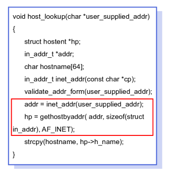
((a))

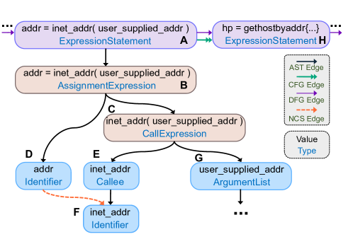
((b))

Figure 1: (a) is a source code snippet of CWE-476. (b) is a visualisation of the code structure graph of the statements highlighted in red box in (a). Each node is represented with two attributes: Value (described in the first line) and Type (descried in the second line). The nodes with different shades indicate different node types.

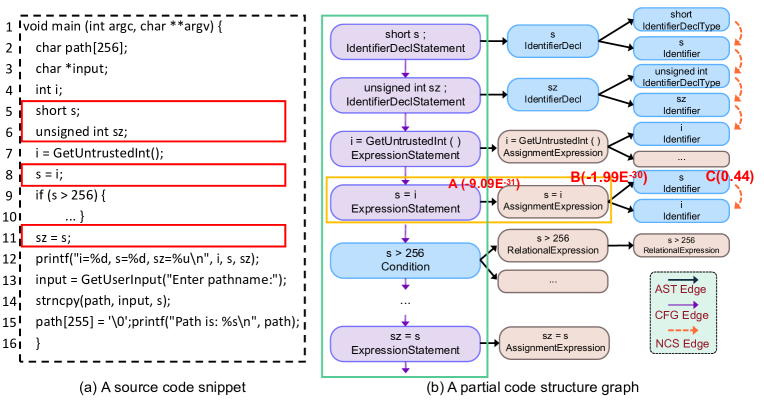
Figure 2: (a) is a source code snippet of CWE-839 [38]. (b) is the code structure graph generated from the source code snippet. The red box statement indicates the vulnerable statement. The orange box denotes the same node value and different node types. The green box indicates that GNN needs to use more than six message-passing steps to capture the long dependencies between vulnerability statements. The red font denotes the meta-path between two nodes, and the brackets indicate the meta-path weight of the path learned in this example.

2.1 Code Structure Graph

Code structure graphs are widely used in code vulnerability detection. Devign [14] uses code structure graph, which shares the same node set with AST and merges the edge sets of AST, CFG, DFG, and natural code sequence (NCS). Fig.1(b) shows a code snippet of CWE-476 [39] and the corresponding code structure graph. As shown in Fig.1(b), besides different edge types, each input node is represented with two attributes: Value (described in the first line) and Type (described in the second line).

The code structure graph encompasses a wealth of both syntactic and semantic information of the source code. Following the previous work [18, 14], we use the Word2Vec [40] to capture the semantic associations within each node vector. However, the current DL-based vulnerability detection approaches exhibit limitations in effectively exploiting syntactic information. For example, IVDetect [19] primarily focuses on combining node types into the node vector, while ignoring the heterogeneous relations, i.e., jointly considering different types of nodes and edges. Devign [14] treats all nodes as the same node type in the Gated Graph Neural Network.

Compared with natural languages, the source code exhibits greater regularity and logical structure [14], meaning that alterations in specific semantic information, such as variable names and identifiers [41], do not necessarily result in vulnerabilities. These heterogeneous relations reflect the diverse relationships across various node and edge types, thereby benefiting the acquisition of vulnerability patterns. By employing the heterogeneous relations, we can gain deep insights into the variations in node types which are important code structural information [42]. In this paper, we aim at exploiting the heterogeneous relations for vulnerability detection by defining meta paths.

2.2 Graph Neural Networks

Graph Neural Networks (GNNs) have been widely used in the software engineering tasks, such as code classification [43], code clone detection [44, 45, 46], etc. This is due to the inherent ability to capture the structural information of source code [18]. GNNs generally aggregate neighbouring nodes’ information and use message passing for passing information from the current node to other nodes, finally forming a graph representation.

Several GNN-based methods have been proposed for vulnerability detection. For instance, Devign [14] learns the code structure information by adopting Gated Graph Neural Network (GGNN) to process multiple edge types graphs. Reveal [18] aims at offering a better separability between vulnerable and non-vulnerable samples by using GGNN and multi-layer perceptron (MLP). IVDetect [19] uses the feature-attention GCN model to learn the source code representation, achieving state-of-the-art performance. Despite the good performance, the existing methods still struggle to effectively capture long-range dependencies. Previous studies [31, 32] have demonstrated that Graph Neural Networks (GNNs) are limited to learning information from neighboring nodes. In vulnerability detection datasets, the average distance between nodes in different datasets is approximately seven. However, certain traditional GNNs, such as the Graph Convolutional Network, achieve optimal performance with only two layers [32]. Consequently, these models can only capture information from nodes with a distance of less than two, which is inadequate for capturing vulnerability patterns. Wang et al. [29] further highlight the challenge of learning long-distance dependencies in code structure graphs, which often have multiple levels and a significant number of nodes.

To illustrate, Fig. 2 shows a portion of the code from line 5 to line 11. In Fig. 2(a), the three statements highlighted in red boxes (lines 5, 8, and 11) are the root cause of the vulnerability. In the corresponding code structure graph in Fig. 2(b), the green box indicates that more than six steps of message-passing are required in a GNN to capture the long dependencies between vulnerability statements. Consequently, the model faces difficulties in effectively capturing vulnerability patterns from the code structure graph.

In addition, to evaluate the situation of long-range dependencies, we employ Devign [14] as a case study and examine the correlation between model performance and the number of graph nodes. Each node in CFG represents a node, and the average distance between nodes will grow as the number of nodes increases [47]. Our investigation centers on the Reveal dataset [18], and we partition into five intervals based on the number of nodes in code structure graphs, with results shown in Table I. Notably, Devign exhibits superior performance for graphs with a lower node count, achieving an accuracy of 90.71% for graphs containing no more than 50 nodes. However, its performance declines significantly as the number of nodes increases. For graphs with more than 200 nodes, Devign’s accuracy drops to approximately 54.17%. In this paper, we propose a multi-granularity attention mechanism for learning the long-range dependencies.

TABLE I: The accuracy of Devign [14] and MAGNET on the Reveal dataset [18] with different numbers of graph nodes.

Node number	[0,50]	(50,100]	(100,150]	(150,200]	>200
Devign	90.71	76.86	56.67	57.50	54.17
MAGNET	96.59	98.64	94.92	94.62	90.88

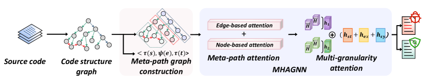
Figure 3: The architecture of MAGNET.

TABLE II: Classification of node types.

Node type	Classification	Type Number
Statement	Statement, SwitchStatement, DoStatement, GotoStatement, WhileStatement, BreakStatement, CompoundStatement, ForStatement, ReturnStatement, IdentifierDeclStatement, TryStatement, ClassDefStatement, ContinueStatement, IfStatement, ExpressionStatement, ElseStatement, DeclStatement	17
Expression	Expression, InclusiveOrExpression, MultiplicativeExpression, AssignmentExpression, UnaryOperationExpression, SizeofExpression, OrExpression, ShiftExpression, RelationalExpression, CallExpression, CastExpression, ConditionalExpression, OperationExpression, EqualityExpression, AdditiveExpression, PrimaryExpression, AndExpression, ExclusiveOrExpression, BitAndExpression, UnaryExpression	20
Symbol	Symbol, File, IncDec, ForInit, SizeofOperand, PtrMemberAccess, Sizeof, IdentifierDeclType, IdentifierDecl, ClassDef, ParameterList, Callee, Condition, ArrayIndexing, ArgumentList, Parameter, Argument, ParameterType, CastTarget, Function, ReturnType, Label, FunctionDef, MemberAccess, InitializerList, CFGErrorNode, InfiniteForNode, CFGExitNode, CFGEntryNode, Identifier, Decl	32

2.3 Meta-path

The meta-path has been used in social networks areas [48], which is a path consisting of a sequence of edge types in the heterogeneous graph. The heterogeneous graph contains multiple types of nodes or multiple types of edges with the data structure as a directed graph, where two nodes can be connected via different edges. In vulnerability detection, the code structure graph is also a heterogeneous graph. For example, the previous methods treat the paths AB and AH as the same type path. In the heterogeneous graph, two nodes A and B can be connected via the “ExpressionStatement-AST-AssignmentStatement” meta-path in Fig. 1(b), which is different from the meta-path “ExpressionStatement-CFG-ExpressionStatement” connected between nodes A and H. Constructing the meta-path in the heterogeneous network can capture the structure information among nodes in the code structure graph. As shown in Figure 2(a), we observe that Line 8 represents a vulnerability statement of source code, as denoted by the orange box containing two nodes in Figure 2(b). These two nodes possess distinct types even though they share the same node value of “s=i”. Specifically, the left node corresponds to the “ExpressionStatement” type, signifying the statement property, while the right node pertains to the “AssignmentExpression” type, representing the expression property. These nodes are connected by an AST edge, forming a heterogeneous relation. In this paper, we construct the $<ExpressionStatement,AST,AssignmentExpression>$ meta-path to exploit the structural information in the code structure graph, which captures the heterogeneous relations to facilitate vulnerability detection. Without considering the heterogeneous relations which contain rich structural information within the source code, the previous methods tend to fail for vulnerability detection. In this paper, we demonstrate the impact of heterogeneous relations on code vulnerability detection. After the model is trained, it adjusts the weights of different heterogeneous relationships, causing the model to focus its attention on specific paths.

3 Proposed Model

In this section, we introduce the overall architecture of MAGNET. As shown in Fig. 3, the architecture includes two main components: (1) multi-granularity meta-path graph construction, aiming at constructing heterogeneous relations as meta paths. (2) meta-path based hierarchical attentional graph neural network, aiming at learning the representations of the meta-path graph.

3.1 Multi-granularity Meta-path Graph Construction

In this section, we first illustrate how to group the node types into multiple granularities, and then describe how we construct the meta-path graph.

3.1.1 Node Type Grouping

Directly employing the node types provided by the parsing principles [21] would lead to an increasingly large number of heterogeneous relations. For example, following Reveal [18], each dataset can be parsed into 69 node types, resulting in more than 10,000 heterogeneous relations. Prior research [36] demonstrates that GNN models tend to get underfitting on complex heterogeneous relations. To mitigate the issue, we propose to group the node types into three different granularities, including “Statement”, “Expression” and “Symbol”.

Specifically, according to the code parsing principles [21] we group all node types into the following three categories: (1) nodes at “Statement” granularity: the node represents the whole sentence in a code snippet, e.g., node A and node H in Fig. 1(b). (2) nodes at “Expression” granularity: the node consists of two or more operator/operands [49], e.g, the brown-shaded node B and C in Fig. 1(b). (3) nodes at “Symbol” granularity: the remaining nodes are categorized as “Symbol” nodes for simplicity, e.g., the nodes D, E, F and G in Fig. 1(b).

The node types at each granularity are illustrated in Table II, from coarse-grained $Statement$ category to fine-grained $Symbol$ category. The granularity-related categories reflect the structural information of the node value and can facilitate the subsequent DL-based learning process.

3.1.2 Meta Path Construction

The code structure graph $\mathcal{G}$ is a direct graph, indicated as $\mathcal{G}(\mathcal{V},\mathcal{E},\mathcal{A},\mathcal{R})$, where $\mathcal{V}$, $\mathcal{E}$, $\mathcal{A}$, and $\mathcal{R}$ represent the node set, edge set, node type set, and edge type set, respectively. Each node $v\in\mathcal{V}$ has its associated type with the mapping function $\tau(v):\mathcal{V}\rightarrow\mathcal{A}$. Each edge $e\in\mathcal{E}$ is associated with a type, with the mapping function: $\psi(e):\mathcal{E}\rightarrow\mathcal{R}$. The edge $e=(s,t)$ denotes the path linked from source node $s\in\mathcal{V}$ to target node $t\in\mathcal{V}$. To capture the structural information of heterogeneous relations between nodes at different granularity, we propose to build meta paths. Based on the grouped $t_{n}$ node types ($t_{n}=3$, i.e., $Statement$, $Expression$ and $Symbol$) and contained $t_{e}$ edge types ($t_{e}=4$, i.e., $AST$, $CFG$, $DFG$ and $NCS$), we define a meta path as below.

Definition 1 (meta path)

A meta path on the code structure graph is denoted as a triplet $(\tau(s),\psi(e),\tau(t))$, indicating a heterogeneous relation from source node $s$ to a target node $t$ with a connection edge $e$. $\tau(\cdot)$ denotes the type category of the corresponding node, and $\psi(e)$ means the type of the edge $e$.

The maximum number of types for the meta paths is $t_{n}^{2}*t_{e}=36$. We then analyze the distribution of heterogeneous relations belonging to different meta-path types. Fig. 4 illustrate the results on the FFMPeg+Qemu dataset, and the other datasets show a similar distribution trend. As can be seen, the last four types of the total 36 types, e.g., $(Ex,2,Ex)$, $(Ex,2,St)$, appear fewer than three times in the dataset. To facilitate the representation learning of the heterogeneous relations in the graph, we filter out the rare types [50, 51], and employ the remaining 32 types of meta paths for constructing the meta-path graph. For the two nodes that have more than one meta path, we keep the multiple meta paths, e.g., nodes A and H in Fig. 1(b) have $(St,DFG,St)$ and $(St,CFG,St)$ meta-paths; thus, the structure information of the code strucure graph can be maintained by constructing meta-path graph.

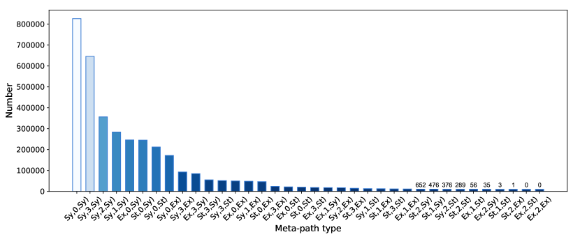
Figure 4: Distribution of different types of meta paths on FFMPeg+Qemu dataset. ‘$St$’ , ‘$Ex$’ and ‘$Sy$’ denote the ‘$Statement$’, ‘$Expression$’ and ‘$Symbol$’ types of nodes. ‘0’, ‘1’, ‘2’, and ‘3’ represent ’AST’, ‘DFG’, ‘CFG’ and ‘NCS’ type edges, respectively. The x-axis indicates the type of meta-path, and the y-axis indicates the number of each meta-path.

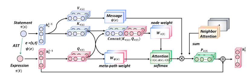
Figure 5: The architecture of meta-path attention.

3.2 Meta-path based Hierarchical Attentional Graph Neural Network

In this section, we illustrate the proposed meta-path based hierarchical attentional graph neural network, named MHAGNN. MHAGNN consists of two modules: (1) a meta-path attention mechanism for capturing the representations of heterogeneous relations; and (2) a multi-granularity attention mechanism for capturing long-range dependency in the meta-path graph.

3.2.1 Meta-path Attention Mechanism

To better utilize the heterogeneous relations, i.e., triplets $(\tau(s),\psi(e),\tau(t))$, from the constructed multi-granularity meta-paths, we devise a meta-path attention mechanism, with detailed architecture presented in Fig. 5. The meta-path attention consists of node-based attention and edge-based attention, which aims at learning the importance of different node types and different edge types in the graph structure representation.

Node-based attention: The node-based attention score $Att_{node}^{l}$ for the target node $t$ in the $l$-th layer is defined as follows:

$$Att_{node}^{l}=\sigma\left(W^{l}_{\tau(t)}\cdot\left({K^{l}}(s)||{Q^{l}}(t)\right)\right)$$ (1)

$$K^{l}{(s)}=Linear_{\tau(s)}(h_{s}^{l-1})$$ (2)

$$Q^{l}{(t)}=Linear_{\tau(t)}(h_{t}^{l-1})$$ (3)

where $W^{l}_{\tau(t)}$ is a trainable weight matrix, indicating the contribution of node type $\tau(t)$ to the representation of the whole graph. The symbol $||$ is the concatenation operation and $\sigma$ is the sigmoid activation function. $Q^{l}{(t)}$ and $K^{l}{(s)}$ are the linear projection of node vector $h^{l-1}_{t}$ and $h^{l-1}_{s}$, respectively, which are used to learn the textual information of the code. $Q^{l}{(t)}$ and $K^{l}{(s)}$ are the linear projection of node $t$ and $s$, respectively. In Equation (3) and (2), $Linear$ denotes a fully connected neural network layer. $h_{t}^{l-1}$ and $h_{s}^{l-1}$ denote the node vectors of $t$ and $s$ in $(l-1)$-th layer, respectively, where $h_{t}^{0}$ and $h_{s}^{0}$ are initialized as 100-dimensional vector by word2vec [40].

Edge-based attention: The edge-based attention score $Att_{edge}^{l}$ for the target node $t$ is defined as following:

$$Att_{edge}^{l}=\left({K^{l}}(s){W_{\psi(e)}}{Q^{l}}(t)^{T}\right)\cdot\frac{\mu(\psi(e))}{\sqrt{\frac{d}{h}}}$$ (4)

where $W_{\psi(e)}$ and $\mu(\psi(e))$ denote the trainable matrix and parameter for each edge type $\psi(e)$, representing the importance of the edge type to the source node $s$ and the target node $t$, respectively. $d$ and $h$ denote the vector dimension and the number of edge-based attention heads, respectively.

Meta-path attention: Based on the computed node-based attention and edge-based attention, we devise the meta-path attention score $Att_{(\tau(s),\psi(e),\tau(t))}^{l}$ for the target node $t$ to model the heterogeneity of the relationship $(\tau(s),\psi(e),\tau(t))$:

$$Att_{(\tau(s),\psi(e),\tau(t))}^{l}=softmax\left(\|_{1}^{H}\left(Att_{edge}^{l}+Att_{node}^{l}\right)\right)$$ (5)

where $||_{1}^{H}$ represents the concatenation of $H$ attention heads.

Finally, we sum the attention scores of all neighbor nodes connected to the node $t$, which is used as the meta-path attention score of the node $t$. We treat meta-path attention score $Att_{(\tau(s),\psi(e),\tau(t))}^{l}$ as input and utilize message passing from source nodes to the target nodes, which incorporates the heterogeneous relations into $l$-th layer’s. To enhance the ability of GNN to represent different nodes, we also establish a residual connection [52] with the previous $(l-1)$-th layer’s output, and get the updated node vector $h^{l}_{t}$ as:

$$h_{t}^{l}=\sigma{\left(\sum_{s\in N_{t}}Att_{(\tau(s),\psi(e),\tau(t))}^{l}\cdot{V^{l}}(s)\right)}+h_{t}^{(l-1)}$$ (6)

$$V^{l}{(s)}=Linear_{\tau(s)}(h_{s}^{l-1})$$ (7)

where $N_{t}$ denotes the set of neighboring nodes of node $t$ and $h_{s}^{l-1}$ denotes the vector representation of the node $s$ in $(l-1)$-th layer. $V^{l}{(s)}$ is also the linear projection of node $s$.

3.2.2 Multi-granularity Attention

To enhance the representations of nodes at different granularities, we propose to adopt both the average-pooling layer and the max-pooling layer simultaneously. The average-pooling layer [53] is designed to capture the long-range dependency in the meta-path graph; while the max-pooling layer aims at magnifying the contribution of the key nodes considering that only few nodes in the graph are vulnerability-related [54]. The multi-granularity attention score $M$ is calculated as below:

$$M=\sigma\left(MLP\left(\omega_{1,i}\cdot AvgPool(F_{i})+\omega_{2,i}\cdot MaxPool(F_{i})\right)\right)$$ (8)

$$(i=st,ex,sy)$$

where $\omega$ denotes a trainable weight for different levels average-pooled and max-pooled features and $i$ denotes different levels (i.e., granularities) of nodes. $F_{st}$, $F_{ex}$, $F_{sy}$ are the node type representation of “Statement”, “Expression” and “Symbol”, respectively, which are calculated as $F_{i}=\left\{{h_{t}}\right\}_{q=1}^{\left|\mathcal{V}_{i}\right|},(i=st,ex,sy)$. $\left|\mathcal{V}_{i}\right|$ denotes the number of a single node types in the whole graph. The single node vector $h_{t}$ is concatenated by bidirectional GRU [55], calculated as $h_{t}=\left(\overrightarrow{GRU}\left(h_{t}^{l}\right)\right)||\left({\overleftarrow{GRU}\left(h_{t}^{l}\right)}\right)$. Finally, we use the typical CrossEntropy loss function [56] for vulnerability prediction.

4 Evaluation

4.1 Research Questions

We evaluate the MAGNET with the state-of-the-art vulnerability methods and aim at answering the following questions:

1. How does our method MAGNET perform in vulnerability detection?

2. What is the impact of different modules in MHAGNN on the detection performance of MAGNET?

3. How effective is MAGNET for detecting Top-25 Most Dangerous CWE?

4. What is the influence of hyper-parameters on the performance of MAGNET?

4.2 Experiment Setup

4.2.1 Dataset

TABLE III: Statistics of the datasets.

Dataset	Samples	Ratio (#Vul:#Non-vul)	Language
FFMPeg+Qemu [14]	22,361	1:1.2	C
Reveal [18]	18,169	1:9.9	C/C++
Fan et al. [37]	179,299	1:16	C/C++

TABLE IV: Comparison results between MAGNET and the baselines on the three datasets. “-” means that the baseline does not apply to the dataset in this scenario. The best result for each metric is highlighted in bold. The shaded cells represent the performance of the top-3 best methods in each metric. Darker cells represent better performance.

	FFMPeg+Qemu [14]				Reveal [18]				Fan et al.. [37]
Baseline	Accuracy	Precision	Recall	F1 score	Accuracy	Precision	Recall	F1 score	Accuracy	Precision	Recall	F1 score
VulDeePecker	49.61	46.05	32.55	38.14	76.37	21.13	13.10	16.17	81.19	38.44	12.75	19.15
Russell et al.	57.60	54.76	40.72	46.71	68.51	16.21	52.68	24.79	86.85	14.86	26.97	19.17
SySeVR	47.85	46.06	58.81	51.66	74.33	40.07	24.94	30.74	90.10	30.91	14.08	19.34
Devign	56.89	52.50	64.67	57.95	87.49	31.55	36.65	33.91	92.78	30.61	15.96	20.98
Reveal	61.07	55.50	70.70	62.19	81.77	31.55	61.14	41.62	87.14	17.22	34.04	22.87
IVDetect	57.26	52.37	57.55	54.84	-	-	-	-	-	-	-	-
MAGNET	63.28	56.27	80.15	66.12	91.60	42.86	61.68	50.57	91.38	22.71	38.92	28.68

In the experiments, we conduct MAGNET on three vulnerability datasets, i.e., FFMPeg+Qemu [14], Reveal [18], and Fan et al. [37]. The statistics of the three datasets are listed in detail in Table III. The FFMPeg+Qemu dataset was proposed by Devign [14], which contains 10+k vulnerable and 12+k non-vulnerable entries. It is a relatively balanced dataset and 45.0% of the samples are vulnerable. The Reveal and Fan et al. datasets are imbalanced, which contain +18k samples with 9.16% vulnerable and +179k samples with 5.88% vulnerable samples. For the programming languages, FFMPeg+Qemu only comes from open-source C projects, and the others datasets collect open-source C/C++ projects.

4.2.2 Baseline Methods

We consider the token-based methods and graph-based methods in vulnerability detection. We implement the baselines and their corresponding parameter settings based on the original papers as much as possible. Since Devign [14] did not publish their source code and parameter settings, we used the repository reproduced by Reveal [18].

Token-based methods: VulDeePecker [17] splits source code into program slices with control dependencies incorporated. The program slices are fed into the model built with an LSTM and attention mechanism. Russell et al. [25] embed the labeled source code into the corresponding matrix. They detect code vulnerabilities by CNN, integrated learning, and random forest classifiers. SySeVR uses multiple code features as input (i.e., code statements, program dependencies, and program slices) and utilizes a bidirectional RNN for code vulnerability detection.

Graph-based methods: Devign [14] uses the GGNN approach on the code structure graph for vulnerability detection. Reveal [18] uses Code Structure Graph (CPG) as the input and leverages GGNN in the feature extraction step. And it combines MLP and Triplet Loss during the training phase. IVDetect [19] constructs the Program Dependency Graph (PDG) and uses GCN to learn the graph representation for capturing vulnerable pattern.

4.2.3 Implementation

We implement our model MAGNET in Python 3.7 using PyTorch [57] and Deep Graph Library (DGL) [58]. We train our model with the NVIDIA GeForce RTX 3090 GPU, installed with Ubuntu 20.04 and CUDA 11.4. In the embedding layer, the initial input dimension $d$ is set to 100 and the hidden state dimension is set to 64. The number of MHAGNN layers is set to 2 and the head of meta-path attention is set to $h$ = 4. We adopt Adam optimizer [59] to train our model with a learning rate $5e^{-4}$. The batch sizes for FFMPeg+Qemu, Reveal, and Fan et al. datasets are set as 512, 512 and 256, respectively.

In addition, to ensure the fairness of the experiments, we use the same data splitting for all baseline approaches as MAGNET. We randomly partition the dataset into disjoint train, valid, and test sets with the ratio of 8:1:1.

4.3 Evaluation Metrics

We use the following four widely-used evaluation metrics to measure our model’s performance:

Precision: Precision is the percentage of true vulnerabilities among the vulnerabilities retrieved. $TP$ and $FP$ are the number of true positives and false positives, respectively.

$$Precision=\frac{TP}{TP+FP}$$ (9)

Recall: Recall is the percentage of vulnerabilities that are retrieved out of all vulnerable samples. $TP$ and $FN$ are the number of true positives and false negatives, respectively.

$$Recall=\frac{TP}{TP+FN}$$ (10)

F1 score: F1 score is the harmonic mean of precision and recall metrics.

$$F1\ score=2\times\frac{Precision\times Recall}{Precision+Recall}$$ (11)

Accuracy: Accuracy is the percentage of correctly classified samples to all samples. $TN$ is the number of true negatives and $TP+TN+FN+FP$ represents the all samples.

$$Accuracy=\frac{TP+TN}{TP+TN+FN+FP}$$ (12)

5 Experimental Result

5.1 RQ1: How does our method MAGNET perform in vulnerability detection?

To answer this research question, we first explore the performance of MAGNET and compare it with other baseline methods. Then, we visualize the features learned by the MAGNET to verify the validity of the learned vulnerability patterns.

5.1.1 Effectiveness of MAGNET

Table IV shows the overall results of all baseline models and MAGNET on the four evaluation metrics. Overall, MAGNET achieves better results and outperforms all of the six referred token-based and graph-based approaches on FFMPeg+Qemu, Reveal and Fan et al. dataset in terms of F1 score by 6.32%, 21.50% and 25.40%, respectively. For the four performance metrics on the three datasets, MAGNET has the best performance in 10 out of the 12 cases. Compared with the best-performing baseline Reveal, our method obtains an average performance improvement of 6.84%, 23.04%, 9.53% and 17.74% on the four metrics, respectively.

We observe that MAGNET outperforms all the baseline methods on the three datasets in terms of F1 score and recall metric. Compared with the best-performing baseline method, MAGNET achieves an average absolute improvement of 6.23% with respect to the F1 score on the three datasets. MAGNET also improves the recall metric by 13.37%, 0.88% and 14.34%, respectively, over the best baseline methods. Such improvement benefits the scenario of vulnerability detection, since a higher recall indicates a larger percentage of vulnerabilities that can be detected.

MAGNET achieves the best performance on all metrics for the FFMPeg+Qemu and Reveal datasets. However, on the Fan et al. dataset, it performs worse than the IVDetect. We believe that this may be due to the class imbalance problem [18] of the Fan et al dataset. MAGNET focuses more on vulnerabilities, which makes it higher on the Recall metric. In addition, in Table IV, the symbol “-” indicates that IVDetect could not converge on the Reveal and Fan et al. datasets, and would identify all code snippets as non-vulnerable when they use the same split setting with MAGNET. The reason may be attributed to that IVDetect is designed for balanced training datasets in the original paper [19], and tends to fail for the commonly-used imbalanced datasets such as the Reveal and Fan et al. datasets.

Experimental results also show that three graph-based methods Devign, Reveal and IVDetect outperform the three token-based methods. For example, the gray cells represent the top-3 best results in the FFMPeg+Qemu dataset appear 6 times in the graph-based methods but only twice in the token-based methods. The reason may be attributed to that token-based methods are more advantageous in capturing the sequence information of codes while ignoring the structural information. In contrast, graph-based methods can better capture code structure information, which is beneficial for vulnerability detection.

5.1.2 Result Visualization

To further analyze the effectiveness of MAGNET, we visualize the representations learnt by MAGNET via the popular t-SNE technique [60]. For comparison, we also use t-SNE to visualize existing graph-based code vulnerability detection methods as well. In the t-SNE space, a larger distance between different classes (i.e., vulnerable and non-vulnerable examples) of nodes indicates a clear and greater separability of classes, which leads to a higher performance of vulnerability detection. In addition, to facilitate the quantification, we use centroids distance $D$ [61] for quantitatively illustrating the separability between different classes.

The feature visualization graphs of t-SNE for the existing graph-based models are shown in Fig. 6(a) to 6(c). It shows that the positive and negative samples in Devign are thoroughly mixed, with the central distance at only 0.0108. Compared with Devign, both Reveal and IVDetect obtain larger central distances, and the scatter appears more dispersed but still lacks the separability visible to the naked eye. In Fig. 6(d), we show the separability of our MAGNET. We can observe that the left side aggregates more vulnerability samples, while the right side has more non-vulnerable examples. Besides, MAGNET shows the largest central distance at 0.2901 among all the methods. The visualization further demonstrates the effectiveness of MAGNET in distinguishing vulnerable code from non-vulnerable code.

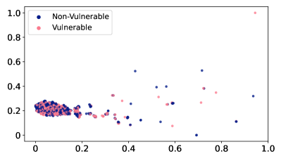
((a))

((b))

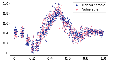
((c))

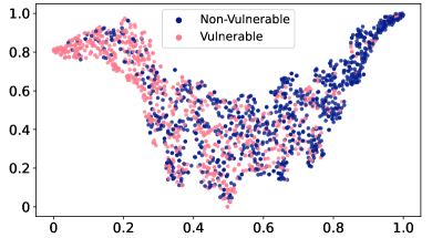
((d))

Figure 6: The t-SNE [60] plot illustrates the distribution between vulnerable (pink) and non-vulnerable (dark blue) examples in the code representations of the different approaches. $D$ indicates the centroids distance between the centers of the vulnerable and non-vulnerable examples.

5.2 RQ2: What is the impact of different modules of MHAGNN?

To answer this research question, we explore the effect of each module in MHAGNN on the performance of MAGNET by performing ablation study on all three datasets.

TABLE V: Results of ablation study.

	FFMPeg+Qemu [14]				Reveal [18]				Fan et al.. [37]
Metrics	Accuracy	Precision	Recall	F1	Accuracy	Precision	Recall	F1	Accuracy	Precision	Recall	F1
w/o edge-att	61.16	55.96	69.52	62.01	91.02	39.60	55.14	46.09	90.54	19.57	36.15	25.39
w/o node-att	60.97	55.97	62.70	59.15	90.89	39.62	58.88	47.37	91.27	19.47	30.62	23.80
w/o multi-att	60.94	55.77	60.92	58.23	88.41	31.22	55.14	39.86	86.27	12.92	36.31	19.06
MAGNET	63.28	56.27	80.15	66.12	91.60	42.86	61.68	50.57	91.38	22.71	38.92	28.68

We construct the following three variations of MAGNET for comparison: (1) without edge-based attention (denoted as w/o edge-att): we remove the edge-based attention to validate the impact of the edge-based attention; (2) without node-based attention (denoted as w/o node-att): we remove the node-based attention to verify the impact of node-based attention; (3) without the multi-granularity attention (denoted as w/o multi-att): we obtain the graph representation through simply summing the node feature embeddings instead of using the proposed multi-granularity attention.

The results of the different variants are shown in Table V. We find that the performance of all the variants is lower than that of MAGNET, which indicates that all the modules contribute to the overall performance of MAGNET. Specifically, without the edge-based attention, the results of accuracy, precision, recall and F1 score on the three datasets drop by 1.18%, 2.24%, 6.65%, and 3.57% on average, respectively. Without node-based attention, the four metrics decrease by 1.04%, 2.26%, 9.52%, and 5.02%, respectively. The node-based attention and edge-based attention contribute greatly to the model performance, since they capture different types of structural information in the meta-path graph.

Among all the three parts, the multi-granularity attention layer contributes the most to the overall performance, which improves the F1 score by 11.93%, 21.18%, and 33.54% on the three datasets, respectively. The reason may be attributed to that the multi-granularity attention facilitates the learning process of global long-range dependency, and can better capture the patterns of vulnerable code.

5.3 RQ3: How effective is MAGNET for Top-25 Most Dangerous CWE?

TABLE VI: The accuracy of baseline and MAGNET for the top-25 most dangerous CWEs. Due to the small number of partial vulnerabilities, we only show the types of vulnerabilities with more than 50 samples. Percentage indicates the proportion of vulnerabilities in the samples.

CWE Type	Percentage	Devign	Reveal	IVDetect	MAGNET
CWE-787	3.34%	45.37	51.71	56.60	83.19
CWE-79	1.16%	39.13	65.22	51.43	71.79
CWE-125	8.61%	47.14	52.54	61.08	72.86
CWE-20	23.48%	42.00	53.58	57.88	75.32
CWE-416	11.78%	46.67	58.13	61.05	72.97
CWE-22	0.77%	56.86	47.06	48.00	64.00
CWE-190	3.84%	44.11	52.47	59.20	76.34
CWE-287	0.72%	35.14	48.65	51.28	71.43
CWE-476	5.33%	48.00	49.41	63.22	73.54
CWE-119	28.61%	43.77	51.23	60.83	77.07
CWE-200	9.02%	44.59	51.18	56.17	76.82
CWE-732	1.64%	34.38	56.25	43.75	76.67
Average		44.38	52.26	59.24	75.70

Common Weakness Enumeration (CWE) [62] is a list of vulnerability weakness types, which serves as a common language for describing and identifying vulnerabilities. The Top-25 most dangerous CWEs list officially publishes the most common and impactful software vulnerabilities over the previous two calendar years based on Common Vulnerabilities and Exposures (CVE) data [63]. Such weaknesses are dangerous compared to other vulnerabilities because they are more numerous and have a higher risk factor (CVSS). In order to explore the effectiveness of MAGNET on the most common vulnerabilities, we validate the effectiveness of MAGNET on the Top-25 most dangerous CWEs.

Specifically, we prepare the evaluation set by extracting the samples belonging to the Top-25 List from the Fan et al dataset. The evaluation set is named as Top-CWE dataset for brevity in this paper. The Top-CWE dataset contains 8,989 code functions, and the specific type distribution is shown in Table 5. In terms of quantity, CWE-119 (the Bounds of a Memory Buffer) [64] and CWE-20 (Improper Input Validation) [65] have the largest proportion, with 28.61% and 23.48%, respectively.

We evaluate 12 types of vulnerabilities in the Fan et al. [37] dataset. This is because only 12 of the 25 most threatening types of CWE appear more than 50 times. The remaining 13 data types appear too infrequently and are difficult to evaluate. We build a unified model for all types of vulnerabilities and use a softmax function for testing based on the type of vulnerability. We compare with all the graph-based baselines that have been trained on the FFMPeg+Qemu model.

As shown in Table VI, our MAGNET achieves more than 70% accuracy on all vulnerabilities, with an average improvement of 27.78%, compared to the previous best baselines. It indicates that our method is able to discover different real-world vulnerabilities more accurately. Specifically, our method obtains the highest identification accuracy of 83.19% on CWE-287 (Improper Authentication) [66] among all the types of vulnerabilities detected. In CWE-20 and CWE-119, which account for a large proportion, MAGNET has an accuracy of 75.32% and 77.07%, respectively, showing 30.13% and 26.70% improvement over previous methods, respectively.

5.4 RQ4: What is the influence of hyper-parameters on the performance of MAGNET?

In this section, we explore the impact of two key hyper-parameters on the performance of MAGNET, including the number of layers of MHAGNN and the number of meta-path attention heads.

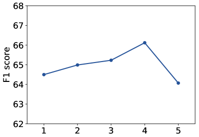
((a))

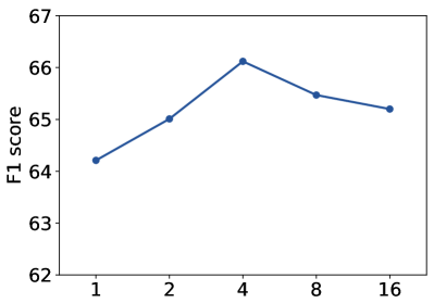
((b))

Figure 7: Parameter analysis of MHAGNN’s layers and head numbers of meta-path attention on the FFMPeg+Qemu dataset.

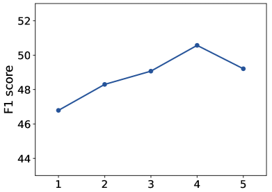
((a))

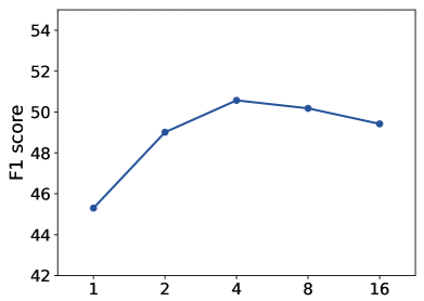
((b))

Figure 8: Parameter analysis of MHAGNN’s layers and head numbers of meta-path attention on the Reveal [18] dataset.

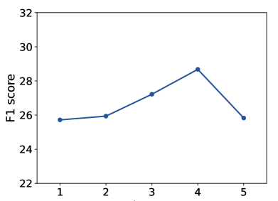
((a))

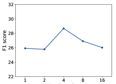
((b))

Figure 9: Parameter analysis of MHAGNN’s layers and head numbers of meta-path attention on the Fan et al. [37] dataset.

5.4.1 Layer Number of MHAGNN

We explore the effect of different numbers of layers in MHAGNN on the performance of MAGNET on the FFMPeg+Qemu and Reveal datasets. Fig. 7(a) and Fig. 8(a) show the F1 score of MAGNET with different numbers of MHAGNN layers. As can be seen, the F1 score of MAGNET first shows an increasing trend and then decreases as the number of layers increases on the FFMPeg+Qemu dataset, with a similar trend observed on the Reveal and Fan et al. datasets. The GNN layers are usually related to the distance between different nodes. The larger the distance between different nodes, the more message passing and GNN layers are required.

We find that MAGNET generally obtains the highest F1 scores when the number of layers is set as four, i.e., 66.12%, 50.57%, and 28.68% on the FFMPeg+Qemu, Reveal and Fan et el. dataset, respectively. We suppose that the MAGNET can better capture the information of the neighborhood as the layer number increases. However, as the layer number further increases, the over-smoothing issue would reduce the model performance.

5.4.2 Attention Head Numbers

We analyze the effect of different attention head numbers on the performance of MAGNET, with the results shown in Fig. 7(b), Fig. 8(b), and Fig. 9(b). As can be seen, MAGNET achieves the optimal F1 score when the number of attention heads is set as four. The trends of parameter setting in head numbers are roughly the same for all datasets. Therefore, we empirically use four head numbers for all three datasets.

Overall, more heads show a significant improvement in F1 score compared to a smaller number of heads, which indicates that more heads are beneficial for capturing the code structure information in the meta-path graph. However, the performance starts to degrade after more than four heads.

6 Discussion

6.1 Case Study

We conduct a case study to further verify the effectiveness of MAGNET in vulnerability detection. For analysis, we visualize the attention weight of each statement produced by MAGNET. Fig. 10 visualizes the heatmap of attention weights for a vulnerable example from CWE-190. In this example, the line 6 is the vulnerable statement, where the sum of the three variables may exceed the maximum value of the short int primitive type, producing a potential integer overflow. MAGNET notices the vulnerability and gives this statement the highest level of attention (red-shaded). The initialization statements (lines 3-5) also present higher attention weights (orange-shaded and red-shaded). From the case, we guess that MAGNET is able to capture the code structural information and patterns of vulnerabilities, which is helpful for detecting code vulnerabilities effectively.

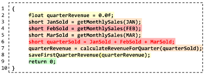
Figure 10: The heatmap of attention weights for a code example from CWE-190 (Integer Overflow or Wraparound). The code in red indicates a vulnerable statement. The red, orange, yellow and green-shaded statements indicate that the corresponding statements are associated with decreasing attention weights.

6.2 Comparison with Pre-trained Models

In recent years, there are some pre-trained approaches e.g., CodeBERT [67], which aim at learning the general program representations. LineVul [13] leverages the CodeBERT model and selects vulnerability detection as the downstream task. And we compare the performance of MAGNET with LineVul. Specifically, we use the officially released code by LineVul and set default hyper-parameters of their paper.

We present a experimental results comparison between our tool (MAGNET) and LineVul, as summarized in Table VII. The results indicate that MAGNET outperforms LineVul in terms of both Recall and F1 metrics on the FFMPeg+Qemu and Reveal datasets, with improvements of 53.92% and 15.02% respectively. This signifies that MAGNET is capable of detecting a greater number of vulnerabilities on these datasets compared to LineVul. On Fan et al. dataset, LineVul outperforms the MAGNET, which we believe may be due to the pre-trained model. However, LineVul uses the pre-trained model, which has additional data and contains more model parameters. Considering the scale of the data using (0.16M of MAGNET and 2.3M of LineVul) and the model parameters containing (0.65M of MAGNET and 125M of LineVul), we believe that MAGNET achieves comparable performance with LineVul.

TABLE VII: Comparison results between MAGNET and the LineVul on the three datasets.

Dataset	FFMPeg+Qemu [14]				Reveal [18]				Fan et al. [37]
Metrics	Accuracy	Precision	Recall	F1 score	Accuracy	Precision	Recall	F1 score	Accuracy	Precision	Recall	F1 score
LineVul	64.75	63.98	50.51	56.45	92.43	48.86	41.35	44.79	98.82	90.68	83.31	86.84
MAGNET	63.28	56.27	80.15	66.12	91.60	42.86	61.68	50.57	91.38	22.71	38.92	28.68

6.3 Performance on the Dataset Split by Time

TABLE VIII: Comparison results between MAGNET and the Reveal on the two settings of split in Fan et al. [37].

Metrics	Accuracy	Precision	Recall	F1 score
Reveal	77.39	12.59	25.73	16.91
MAGNET	84.39	17.01	19.34	18.10

Following the previous work [17, 11, 14, 18, 19], we have repeated three times of the experiment and taken the average to ensure the stability of the results. Furthermore, we employ a more rigorous data partition way to conduct experiments in Fan et al. [37], i.e., splitting data by time. Specifically, we use the “update date” of the vulnerability data in Fan et al.’s dataset as the criterion for the data partition. Specifically, we consider data updated before January 4th, 2018, as the training set, and the data updated from January 4th, 2018, to January 15th, 2019, as the validation set. All samples beyond January 15th, 2019, were allocated to the test set. We compared with the best-performing baseline Reveal to evaluate the influence of the time factor. The detailed experimental results are shown in Table VIII.

It can be seen that based on the division of time, MAGNET gets three better performances out of a total of four cases. This illustrates that MAGNET is able to obtain better experimental results than the best-performing baseline when taking the time factor into consideration. Specifically, MAGNET obtained 7% and 4.42% performance improvements in the Accuracy and Recall metrics, respectively. However, the dataset also suffers from data leakage. In the case of split by time, all four metrics degrade to different degrees. The degradation in the recall metric is the most severe for all methods, reaching an average of 12.96%.

6.4 Effectiveness of the Node Type Grouping Method in MAGNET

TABLE IX: Performance comparison between four variants without node type abstraction in FFMPeg+Qemu [14] datasets.

Node type grouping		Accuracy	Precision	Recall	F1
	Random	60.77	57.73	45.69	51.01
5 node types	Frequency	59.77	54.80	57.05	55.90
	Random	60.88	55.69	61.05	58.25
10 node types	Frequency	61.89	55.66	72.41	62.94
MAGNET		63.28	56.27	80.15	66.12

Using the code structure graph without abstraction in MAGNET is cost intensive. For example, the data preprocessing steps of the FFMPeg+Qemu [14], Reveal [18] and Fan et al. [37] required approximately 17, 9, and 170 hours on NVIDIA GeForce RTX 3090 GPU, respectively. The expenditure of resources and time is a consequence of the excessive number of meta-paths. The code structure graph consists of 69 node types and 4 edge types, resulting in a total of $69\times 4\times 69=19044$ Node-Edge-Node meta-paths. This profusion of meta-paths can lead to the out of CUDA memory issue for model training. To validate the effectiveness of our proposed node type grouping, we generate the code structure graph of node types with other abstraction methods.

Specifically, we use two methods to keep $q$ node types: based on the number of nodes and random selection. We use $q$ for 5 and 10 different node types, resulting in four node type abstraction methods. The maximum number of node types is set as 10, since it results in 400 meta-paths, which is close to maximum CUDA memory capacity of the GPU. The experiments are performed the FFMPeg+Qemu dataset for evaluation. The preprocessing step takes approximately three hours, three times longer than that of our MAGNET. The results also validate the effectiveness of the node type grouping strategy in MAGNET. As shown in Table IX, MAGNET outperforms all the four variant approaches, achieving average improvements of 2.45%, 0.3%, 21.1%, and 9.10% for the accuracy, precision, recall, and F1 score, respectively. Furthermore, the selection strategy based on node frequency showcases notable performance improvements compared with the random selection strategy.

6.5 Effectiveness of Meta-path

In vulnerability detection, the code structure graph is also a heterogeneous graph. Constructing the meta-path in the heterogeneous network can capture the vulnerability-related information among nodes in the code structure graph. MAGNET can adjust the different weights of the meta-path, causing the model to focus its attention on specific paths.

Specifically, in Fig. 2, we denote three meta-paths associated with a statement and its sub-nodes, represented by meta-paths A, B, and C, respectively. Traditional vulnerability detection methods, such as Devign and Reveal, assign equal weights to all the paths, requiring the model to process a large amount of information for learning. This tends to result in inaccurate vulnerability detection. In this case, meta-path C is the most critical in terms of the vulnerability trigger path, as the assignment relations between nodes referred to by NCS determine the vulnerability pattern. After model training, the weight assigned to meta-path C is 0.44, while the weights for the other paths are ignorable ($-9.09E^{-31}$ for the meta-path A and $-1.99E^{-30}$ for the meta-path B). It indicates that the model effectively disregards the less relevant paths and focuses on the more critical part of the vulnerability.

6.6 Threat to Validity

Dataset Partition. None of the existing baseline methods publish their divisions of datasets, so we can not completely reproduce the previous results. Following the data division of previous work [14, 18], we perform a dataset division and reproduce the experimental results based on their articles as much as possible. Reveal and IVDetect use different preprocessing methods, which may lead to inconsistencies in the dataset under the same division. We relied on their source code for the preprocessing work as much as possible. Devign [18] did not publish the source code of their implementation, we reproduce Devign based on Reveal’s [18] implementation version and try to be consistent with the original description.

Generalizability of Other Programming Languages. Our node classification is based on the AST node type in C/C++. Therefore, we only conduct experiments on the C/C++ dataset and do not choose other programming languages such as Java and python. However, the main idea of MAGNET can be generalized to other programming languages because the approach does not rely on language-specific features. We will evaluate MAGNET on more programming languages in our future work.

7 Related Work

Recently, learning-based vulnerability detection has been a significant research problem in software engineering. Depending on how the source code is represented and which type of learning model is utilised, existing technologies can be generally divided into two different types: token-based and graph-based methods.

The token-based methods [17, 25, 11, 68, 69] treat the code as a sequence of tokens, which contain two phases: feature extraction and training. In the feature extraction phase, the token-based methods usually extract token-based features as the model input, which include identifiers, keywords, separators, and operators. These features are usually specified and written by developers and can represent the different line structure [70] of the code. For example, Russell et al. [25] divides each code fragment at the function level and treats them as an individual sample. It generates a lexical token sequence for each function to represent the whole code sample feature set. Code2Seq [68] uses path-context extracted features for each program method and splits code tokens into subtokens. In the training phase, these methods treat source code as sequences via utilizing various deep neural networks. Russell et al. use CNN [71] for code vulnerability detection, concatenating these token features through convolution filters. SyseVR [11] uses GRU [72] to capture the sequence information of the code. Code2Seq uses BiLSTM [73] to encode the necessary information in a sequence of tokens.

In recent years, the graph-based methods [14, 18, 19, 74, 75] have achieved state-of-the-art performance on vulnerability detection. They capture more structural information in the source code than token-based methods. They generally represent source code snippets as graphs generated from static analysis. Depending on different code representations, they design various GNN models for detecting code vulnerabilities. For example, VGDETECTOR [74] uses CFGs to embed the execution order of a code sample and then uses the GCN [26] to capture neighborhood information in the graph structure. Reveal [18] first generate CPG [21] and use Word2Vec [40] to initial the node vector representations of the code tokens. Then they use GGNN [27] to detect code vulnerabilities.

Li et al. [76] propose a bug detection approach that utilizes Program Dependency Graph (PDG) and Data Flow Graph (DFG) as the global context, while leveraging extracted information from the Abstract Syntax Tree (AST) as the local context. They treat the AST as a homogeneous graph, focusing solely on the relationships between different node vectors along paths. The difference between Li et al.’s work and MAGNET is the targeted programming languages. The parsing process in Li et al.’s approach is specifically designed for the Java programming language, which is hard to be applied to C/C++ language.

However, all these methods focus on learning the local features of nodes and fail to capture heterogeneous relations and long-range dependencies among different types of nodes and edges. For example, Devign [14] treats all nodes as the same node type and only uses the node value in the code structure graph, which leads to missing information on the node type and ignoring heterogeneous relations in the code structure graph. Cao et al. [15] construct the Program Dependence Graph (PDG) instead of a code structure graph to capture the interprocedural flow information including data flow and control flow, which only focus on the statement nodes and do not consider the other nodes. In this paper, we propose a meta-path based attentional graph learning model to learn the heterogeneous relations and long-range dependencies in the code structure graph.

8 Conclusion

In this paper, we propose MAGNET, a meta-path based attentional graph learning model for vulnerability detection. MAGNET consists of a multi-granularity meta-path construction, which consider the heterogeneous relations between the different node and edge type. We also propose a multi-level attentional graph neural network MHAGNN to comprehensively capture long-range dependencies and structural information in the meta-path graph. Our experimental results on three popular datasets validate the effectiveness of MAGNET, and the ablation studies and visualizations further confirm the advantages of MAGNET. Compared with state-of-the-art deep learning-based methods, MAGNET gains better performance and detects more vulnerabilities in the real world. The implementation of MAGNET and the experimental data are publicly available at: https://github.com/xmwenxincheng/MAGNET.

References

- [1] S. M. Ghaffarian and H. R. Shahriari, “Software vulnerability analysis and discovery using machine-learning and data-mining techniques: A survey,” ACM Comput. Surv., vol. 50, no. 4, pp. 56:1–56:36, 2017.
- [2] A. Johnson, K. Dempsey, R. Ross, S. Gupta, D. Bailey et al., “Guide for security-focused configuration management of information systems,” NIST special publication, vol. 800, no. 128, pp. 16–16, 2011.
- [3] Y. Wei, X. Sun, L. Bo, S. Cao, X. Xia, and B. Li, “A comprehensive study on security bug characteristics,” J. Softw. Evol. Process., vol. 33, no. 10, 2021.
- [4] Q. Tan, X. Wang, W. Shi, J. Tang, and Z. Tian, “An anonymity vulnerability in tor,” IEEE/ACM Transactions on Networking, vol. 30, no. 6, pp. 2574–2587, 2022.
- [5] Bugcrowd. (2022) 2022 bugcrowd priority one report. [Online]. Available: https://www.bugcrowd.com/resources/reports/priority-one-report/
- [6] Wikipedia. (2021) Log4shell. [Online]. Available: https://en.wikipedia.org/wiki/Log4Shell
- [7] S. Neuhaus, T. Zimmermann, C. Holler, and A. Zeller, “Predicting vulnerable software components,” in Proceedings of the 2007 ACM Conference on Computer and Communications Security, CCS 2007, Alexandria, Virginia, USA, October 28-31, 2007, P. Ning, S. D. C. di Vimercati, and P. F. Syverson, Eds. ACM, 2007, pp. 529–540.
- [8] R. Scandariato, J. Walden, A. Hovsepyan, and W. Joosen, “Predicting vulnerable software components via text mining,” IEEE Trans. Software Eng., vol. 40, no. 10, pp. 993–1006, 2014.
- [9] Y. Shin, A. Meneely, L. A. Williams, and J. A. Osborne, “Evaluating complexity, code churn, and developer activity metrics as indicators of software vulnerabilities,” IEEE Trans. Software Eng., vol. 37, no. 6, pp. 772–787, 2011.
- [10] Y. Wu, D. Zou, S. Dou, W. Yang, D. Xu, and H. Jin, “Vulcnn: An image-inspired scalable vulnerability detection system,” in 44th IEEE/ACM 44th International Conference on Software Engineering, ICSE 2022, Pittsburgh, PA, USA, May 25-27, 2022. ACM, 2022, pp. 2365–2376.
- [11] Z. Li, D. Zou, S. Xu, H. Jin, Y. Zhu, and Z. Chen, “Sysevr: A framework for using deep learning to detect software vulnerabilities,” IEEE Trans. Dependable Secur. Comput., vol. 19, no. 4, pp. 2244–2258, 2022.
- [12] D. Hin, A. Kan, H. Chen, and M. A. Babar, “Linevd: Statement-level vulnerability detection using graph neural networks,” CoRR, vol. abs/2203.05181, 2022.
- [13] M. Fu and C. Tantithamthavorn, “Linevul: A transformer-based line-level vulnerability prediction,” 2022.
- [14] Y. Zhou, S. Liu, J. K. Siow, X. Du, and Y. Liu, “Devign: Effective vulnerability identification by learning comprehensive program semantics via graph neural networks,” in Advances in Neural Information Processing Systems 32: Annual Conference on Neural Information Processing Systems 2019, NeurIPS 2019, 2019, pp. 10 197–10 207.
- [15] S. Cao, X. Sun, L. Bo, R. Wu, B. Li, and C. Tao, “MVD: memory-related vulnerability detection based on flow-sensitive graph neural networks,” CoRR, vol. abs/2203.02660, 2022.
- [16] H. Wang, G. Ye, Z. Tang, S. H. Tan, S. Huang, D. Fang, Y. Feng, L. Bian, and Z. Wang, “Combining graph-based learning with automated data collection for code vulnerability detection,” IEEE Trans. Inf. Forensics Secur., vol. 16, pp. 1943–1958, 2021.
- [17] Z. Li, D. Zou, S. Xu, X. Ou, H. Jin, S. Wang, Z. Deng, and Y. Zhong, “Vuldeepecker: A deep learning-based system for vulnerability detection,” in 25th Annual Network and Distributed System Security Symposium, NDSS 2018, San Diego, California, USA, February 18-21, 2018. The Internet Society, 2018.
- [18] S. Chakraborty, R. Krishna, Y. Ding, and B. Ray, “Deep learning based vulnerability detection: Are we there yet?” CoRR, vol. abs/2009.07235, 2020.
- [19] Y. Li, S. Wang, and T. N. Nguyen, “Vulnerability detection with fine-grained interpretations,” in ESEC/FSE ’21: 29th ACM Joint European Software Engineering Conference and Symposium on the Foundations of Software Engineering, Athens, Greece, August 23-28, 2021. ACM, 2021, pp. 292–303.
- [20] J. K. Siow, S. Liu, X. Xie, G. Meng, and Y. Liu, “Learning program semantics with code representations: An empirical study,” CoRR, vol. abs/2203.11790, 2022.
- [21] F. Yamaguchi, N. Golde, D. Arp, and K. Rieck, “Modeling and discovering vulnerabilities with code property graphs,” in 2014 IEEE Symposium on Security and Privacy, SP 2014. IEEE Computer Society, 2014, pp. 590–604.
- [22] I. Neamtiu, J. S. Foster, and M. Hicks, “Understanding source code evolution using abstract syntax tree matching,” ACM SIGSOFT Softw. Eng. Notes, vol. 30, no. 4, pp. 1–5, 2005.
- [23] X. Huo, M. Li, and Z. Zhou, “Control flow graph embedding based on multi-instance decomposition for bug localization,” in The Thirty-Fourth AAAI Conference on Artificial Intelligence, AAAI 2020, The Thirty-Second Innovative Applications of Artificial Intelligence Conference, IAAI 2020, The Tenth AAAI Symposium on Educational Advances in Artificial Intelligence, EAAI 2020, New York, NY, USA, February 7-12, 2020. AAAI Press, 2020, pp. 4223–4230.
- [24] C. Cummins, Z. V. Fisches, T. Ben-Nun, T. Hoefler, M. F. P. O’Boyle, and H. Leather, “Programl: A graph-based program representation for data flow analysis and compiler optimizations,” in Proceedings of the 38th International Conference on Machine Learning, ICML 2021, 18-24 July 2021, Virtual Event, ser. Proceedings of Machine Learning Research, M. Meila and T. Zhang, Eds., vol. 139. PMLR, 2021, pp. 2244–2253.
- [25] R. L. Russell, L. Y. Kim, L. H. Hamilton, T. Lazovich, J. Harer, O. Ozdemir, P. M. Ellingwood, and M. W. McConley, “Automated vulnerability detection in source code using deep representation learning,” in 17th IEEE International Conference on Machine Learning and Applications, ICMLA 2018, Orlando, FL, USA, December 17-20, 2018, M. A. Wani, M. M. Kantardzic, M. S. Mouchaweh, J. Gama, and E. Lughofer, Eds. IEEE, 2018, pp. 757–762.
- [26] T. N. Kipf and M. Welling, “Semi-supervised classification with graph convolutional networks,” in 5th International Conference on Learning Representations, ICLR 2017, Toulon, France, April 24-26, 2017, Conference Track Proceedings. OpenReview.net, 2017.
- [27] Y. Li, D. Tarlow, M. Brockschmidt, and R. S. Zemel, “Gated graph sequence neural networks,” in 4th International Conference on Learning Representations, ICLR 2016, 2016.
- [28] P. Velickovic, G. Cucurull, A. Casanova, A. Romero, P. Liò, and Y. Bengio, “Graph attention networks,” CoRR, vol. abs/1710.10903, 2017.
- [29] X. Wang, Q. Wu, H. Zhang, C. Lyu, X. Jiang, Z. Zheng, L. Lyu, and S. Hu, “Heloc: Hierarchical contrastive learning of source code representation,” CoRR, vol. abs/2203.14285, 2022.
- [30] W. Min, W. Rongcun, and J. Shujuan, “Source code vulnerability detection based on relational graph convolution network,” Journal of Computer Applications, vol. 42, no. 6, p. 1814, 2022.
- [31] F. Liu, Z. Cheng, L. Zhu, Z. Gao, and L. Nie, “Interest-aware message-passing GCN for recommendation,” in WWW ’21: The Web Conference 2021, Virtual Event / Ljubljana, Slovenia, April 19-23, 2021, J. Leskovec, M. Grobelnik, M. Najork, J. Tang, and L. Zia, Eds. ACM / IW3C2, 2021, pp. 1296–1305.
- [32] U. Alon and E. Yahav, “On the bottleneck of graph neural networks and its practical implications,” in 9th International Conference on Learning Representations, ICLR 2021, Virtual Event, Austria, May 3-7, 2021. OpenReview.net, 2021.
- [33] D. Guo, S. Ren, S. Lu, Z. Feng, D. Tang, S. Liu, L. Zhou, N. Duan, A. Svyatkovskiy, S. Fu, M. Tufano, S. K. Deng, C. B. Clement, D. Drain, N. Sundaresan, J. Yin, D. Jiang, and M. Zhou, “Graphcodebert: Pre-training code representations with data flow,” in 9th International Conference on Learning Representations, ICLR 2021, Virtual Event, Austria, May 3-7, 2021. OpenReview.net, 2021.
- [34] D. Zhu, X. Dai, and J. Chen, “Pre-train and learn: Preserving global information for graph neural networks,” J. Comput. Sci. Technol., vol. 36, no. 6, pp. 1420–1430, 2021.
- [35] Q. Li, Z. Han, and X. Wu, “Deeper insights into graph convolutional networks for semi-supervised learning,” in Proceedings of the Thirty-Second AAAI Conference on Artificial Intelligence, (AAAI-18), the 30th innovative Applications of Artificial Intelligence (IAAI-18), and the 8th AAAI Symposium on Educational Advances in Artificial Intelligence (EAAI-18), New Orleans, Louisiana, USA, February 2-7, 2018. AAAI Press, 2018, pp. 3538–3545.
- [36] Y. Xiong, Y. Zhang, X. Kong, H. Chen, and Y. Zhu, “Graphinception: Convolutional neural networks for collective classification in heterogeneous information networks,” IEEE Trans. Knowl. Data Eng., vol. 33, no. 5, pp. 1960–1972, 2021.
- [37] J. Fan, Y. Li, S. Wang, and T. N. Nguyen, “A C/C++ code vulnerability dataset with code changes and CVE summaries,” in MSR ’20: 17th International Conference on Mining Software Repositories, Seoul, Republic of Korea, 29-30 June, 2020. ACM, 2020, pp. 508–512.
- [38] Cwe-839: Numeric range comparison without minimum check. [Online]. Available: https://cwe.mitre.org/data/definitions/839.html
- [39] Cwe-476: Null pointer dereference. [Online]. Available: https://cwe.mitre.org/data/definitions/476.html
- [40] K. W. Church, “Word2vec,” Nat. Lang. Eng., vol. 23, no. 1, pp. 155–162, 2017.
- [41] M. R. I. Rabin, N. D. Q. Bui, K. Wang, Y. Yu, L. Jiang, and M. A. Alipour, “On the generalizability of neural program models with respect to semantic-preserving program transformations,” Inf. Softw. Technol., vol. 135, p. 106552, 2021.
- [42] H. Zhang, Z. Li, G. Li, L. Ma, Y. Liu, and Z. Jin, “Generating adversarial examples for holding robustness of source code processing models,” in The Thirty-Fourth AAAI Conference on Artificial Intelligence, AAAI 2020, The Thirty-Second Innovative Applications of Artificial Intelligence Conference, IAAI 2020, The Tenth AAAI Symposium on Educational Advances in Artificial Intelligence, EAAI 2020, New York, NY, USA, February 7-12, 2020. AAAI Press, 2020, pp. 1169–1176.
- [43] M. Allamanis, M. Brockschmidt, and M. Khademi, “Learning to represent programs with graphs,” in 6th International Conference on Learning Representations, ICLR 2018, Vancouver, BC, Canada, April 30 - May 3, 2018, Conference Track Proceedings. OpenReview.net, 2018.
- [44] Y. Wu, D. Zou, S. Dou, S. Yang, W. Yang, F. Cheng, H. Liang, and H. Jin, “Scdetector: Software functional clone detection based on semantic tokens analysis,” in 35th IEEE/ACM International Conference on Automated Software Engineering, ASE 2020, Melbourne, Australia, September 21-25, 2020. IEEE, 2020, pp. 821–833.
- [45] W. Wang, G. Li, B. Ma, X. Xia, and Z. Jin, “Detecting code clones with graph neural network and flow-augmented abstract syntax tree,” in 27th IEEE International Conference on Software Analysis, Evolution and Reengineering, SANER 2020, London, ON, Canada, February 18-21, 2020, K. Kontogiannis, F. Khomh, A. Chatzigeorgiou, M. Fokaefs, and M. Zhou, Eds. IEEE, 2020, pp. 261–271.
- [46] W. Hua, Y. Sui, Y. Wan, G. Liu, and G. Xu, “FCCA: hybrid code representation for functional clone detection using attention networks,” IEEE Trans. Reliab., vol. 70, no. 1, pp. 304–318, 2021.
- [47] J. Lu, X. Yu, G. Chen, and D. Cheng, “Characterizing the synchronizability of small-world dynamical networks,” IEEE Trans. Circuits Syst. I Regul. Pap., vol. 51-I, no. 4, pp. 787–796, 2004.
- [48] Y. Sun, J. Han, X. Yan, P. S. Yu, and T. Wu, “Pathsim: Meta path-based top-k similarity search in heterogeneous information networks,” Proc. VLDB Endow., vol. 4, no. 11, pp. 992–1003, 2011.
- [49] P. J. Landin, “The mechanical evaluation of expressions,” The computer journal, vol. 6, no. 4, pp. 308–320, 1964.
- [50] C. Wang, Y. Song, H. Li, M. Zhang, and J. Han, “Unsupervised meta-path selection for text similarity measure based on heterogeneous information networks,” Data Min. Knowl. Discov., vol. 32, no. 6, pp. 1735–1767, 2018.
- [51] W. Ning, R. Cheng, J. Shen, N. A. H. Haldar, B. Kao, X. Yan, N. Huo, W. K. Lam, T. Li, and B. Tang, “Automatic meta-path discovery for effective graph-based recommendation,” in Proceedings of the 31st ACM International Conference on Information & Knowledge Management, Atlanta, GA, USA, October 17-21, 2022, M. A. Hasan and L. Xiong, Eds. ACM, 2022, pp. 1563–1572.
- [52] K. He, X. Zhang, S. Ren, and J. Sun, “Identity mappings in deep residual networks,” in Computer Vision - ECCV 2016 - 14th European Conference, Amsterdam, The Netherlands, October 11-14, 2016, Proceedings, Part IV, ser. Lecture Notes in Computer Science, B. Leibe, J. Matas, N. Sebe, and M. Welling, Eds., vol. 9908. Springer, 2016, pp. 630–645.
- [53] L. Sun, Z. Chen, Q. M. J. Wu, H. Zhao, W. He, and X. Yan, “Ampnet: Average- and max-pool networks for salient object detection,” IEEE Trans. Circuits Syst. Video Technol., vol. 31, no. 11, pp. 4321–4333, 2021.
- [54] S. Woo, J. Park, J. Lee, and I. S. Kweon, “CBAM: convolutional block attention module,” in Computer Vision - ECCV 2018 - 15th European Conference, Munich, Germany, September 8-14, 2018, Proceedings, Part VII, ser. Lecture Notes in Computer Science, V. Ferrari, M. Hebert, C. Sminchisescu, and Y. Weiss, Eds., vol. 11211. Springer, 2018, pp. 3–19.
- [55] D. Bahdanau, K. Cho, and Y. Bengio, “Neural machine translation by jointly learning to align and translate,” in 3rd International Conference on Learning Representations, ICLR 2015, San Diego, CA, USA, May 7-9, 2015, Conference Track Proceedings, Y. Bengio and Y. LeCun, Eds., 2015.
- [56] P. de Boer, D. P. Kroese, S. Mannor, and R. Y. Rubinstein, “A tutorial on the cross-entropy method,” Ann. Oper. Res., vol. 134, no. 1, pp. 19–67, 2005.
- [57] A. Paszke, S. Gross, F. Massa, A. Lerer, J. Bradbury, G. Chanan, T. Killeen, Z. Lin, N. Gimelshein, L. Antiga, A. Desmaison, A. Köpf, E. Z. Yang, Z. DeVito, M. Raison, A. Tejani, S. Chilamkurthy, B. Steiner, L. Fang, J. Bai, and S. Chintala, “Pytorch: An imperative style, high-performance deep learning library,” in Advances in Neural Information Processing Systems 32: Annual Conference on Neural Information Processing Systems 2019, NeurIPS 2019, December 8-14, 2019, Vancouver, BC, Canada, H. M. Wallach, H. Larochelle, A. Beygelzimer, F. d’Alché-Buc, E. B. Fox, and R. Garnett, Eds., 2019, pp. 8024–8035.
- [58] M. Wang, L. Yu, D. Zheng, Q. Gan, Y. Gai, Z. Ye, M. Li, J. Zhou, Q. Huang, C. Ma, Z. Huang, Q. Guo, H. Zhang, H. Lin, J. Zhao, J. Li, A. J. Smola, and Z. Zhang, “Deep graph library: Towards efficient and scalable deep learning on graphs,” CoRR, vol. abs/1909.01315, 2019.
- [59] Z. Zhang, “Improved adam optimizer for deep neural networks,” in 26th IEEE/ACM International Symposium on Quality of Service, IWQoS 2018, Banff, AB, Canada, June 4-6, 2018. IEEE, 2018, pp. 1–2.
- [60] V. der Maaten, Laurens, and H. Geoffrey, “Visualizing data using t-sne.” Journal of machine learning research, vol. 9, no. 11, 2008.
- [61] C. Mao, Z. Zhong, J. Yang, C. Vondrick, and B. Ray, “Metric learning for adversarial robustness,” in Advances in Neural Information Processing Systems 32: Annual Conference on Neural Information Processing Systems 2019, NeurIPS 2019, December 8-14, 2019, Vancouver, BC, Canada, H. M. Wallach, H. Larochelle, A. Beygelzimer, F. d’Alché-Buc, E. B. Fox, and R. Garnett, Eds., 2019, pp. 478–489.
- [62] Cwe. common weakness enumeratio, 2021. [Online]. Available: https://cwe.mitre.org/.
- [63] “2021 cwe top 25 most dangerous software weaknesses”, 2021. [Online]. Available: https://cwe.mitre.org/top25/archive/2021/2021_cwe_top25.html.
- [64] Cwe-119: Improper restriction of operations within the bounds of a memory buffer. [Online]. Available: https://cwe.mitre.org/data/definitions/119.html
- [65] Cwe-20: Improper input validation. [Online]. Available: https://cwe.mitre.org/data/definitions/20.html
- [66] Cwe-287: Improper authentication. [Online]. Available: https://cwe.mitre.org/data/definitions/287.html
- [67] Z. Feng, D. Guo, D. Tang, N. Duan, X. Feng, M. Gong, L. Shou, B. Qin, T. Liu, D. Jiang, and M. Zhou, “Codebert: A pre-trained model for programming and natural languages,” in Findings of the Association for Computational Linguistics: EMNLP 2020, Online Event, 16-20 November 2020, ser. Findings of ACL, T. Cohn, Y. He, and Y. Liu, Eds., vol. EMNLP 2020. Association for Computational Linguistics, 2020, pp. 1536–1547.
- [68] U. Alon, S. Brody, O. Levy, and E. Yahav, “code2seq: Generating sequences from structured representations of code,” in 7th International Conference on Learning Representations, ICLR 2019, New Orleans, LA, USA, May 6-9, 2019. OpenReview.net, 2019.
- [69] V. Nguyen, T. Le, O. Y. de Vel, P. Montague, J. Grundy, and D. Phung, “Information-theoretic source code vulnerability highlighting,” in International Joint Conference on Neural Networks, IJCNN 2021, Shenzhen, China, July 18-22, 2021. IEEE, 2021, pp. 1–8.
- [70] T. Kamiya, S. Kusumoto, and K. Inoue, “Ccfinder: A multilinguistic token-based code clone detection system for large scale source code,” IEEE Trans. Software Eng., vol. 28, no. 7, pp. 654–670, 2002.
- [71] Y. Kim, “Convolutional neural networks for sentence classification,” in Proceedings of the 2014 Conference on Empirical Methods in Natural Language Processing, EMNLP 2014, October 25-29, 2014, Doha, Qatar, A meeting of SIGDAT, a Special Interest Group of the ACL, A. Moschitti, B. Pang, and W. Daelemans, Eds. ACL, 2014, pp. 1746–1751.
- [72] D. Tang, B. Qin, and T. Liu, “Document modeling with gated recurrent neural network for sentiment classification,” in Proceedings of the 2015 Conference on Empirical Methods in Natural Language Processing, EMNLP 2015, Lisbon, Portugal, September 17-21, 2015, L. Màrquez, C. Callison-Burch, J. Su, D. Pighin, and Y. Marton, Eds. The Association for Computational Linguistics, 2015, pp. 1422–1432.
- [73] A. Graves and J. Schmidhuber, “Framewise phoneme classification with bidirectional LSTM and other neural network architectures,” Neural Networks, vol. 18, no. 5-6, pp. 602–610, 2005.
- [74] X. Cheng, H. Wang, J. Hua, M. Zhang, G. Xu, L. Yi, and Y. Sui, “Static detection of control-flow-related vulnerabilities using graph embedding,” in 24th International Conference on Engineering of Complex Computer Systems, ICECCS 2019, Guangzhou, China, November 10-13, 2019, J. Pang and J. Sun, Eds. IEEE, 2019, pp. 41–50.
- [75] Y. Ding, S. Suneja, Y. Zheng, J. Laredo, A. Morari, G. E. Kaiser, and B. Ray, “VELVET: a novel ensemble learning approach to automatically locate vulnerable statements,” in IEEE International Conference on Software Analysis, Evolution and Reengineering, SANER 2022, Honolulu, HI, USA, March 15-18, 2022. IEEE, 2022, pp. 959–970.
- [76] Y. Li, S. Wang, T. N. Nguyen, and S. V. Nguyen, “Improving bug detection via context-based code representation learning and attention-based neural networks,” Proc. ACM Program. Lang., vol. 3, no. OOPSLA, pp. 162:1–162:30, 2019.