Analysis of Inter-Event Times in Linear Systems under Region-Based Self-Triggered Control

Abstract

This paper analyzes the evolution of inter-event times (IETs) in linear systems under region-based self-triggered control (RBSTC). In this control method, the state space is partitioned into a finite number of conic regions and each region is associated with a fixed IET. In this framework, studying the steady state behavior of the IETs is equivalent to studying the existence of a conic subregion that is positively invariant under the map that gives the evolution of the state from one event to the next. We provide necessary conditions and sufficient conditions for the existence of a positively invariant subregion (PIS). We also provide necessary and sufficient conditions for a PIS to be asymptotically stable. Indirectly, they provide necessary and sufficient conditions for local convergence of IETs to a constant or to a given periodic sequence. We illustrate the proposed method of analysis and results through numerical simulations.

I Introduction

Self-triggering is an efficient method for control under resource constraints. In this method, the control update times are opportunistic and implicitly determined by a triggering rule. Thus, understanding inter-event times (IETs) generated by a self-triggering rule is necessary for higher level planning and scheduling for control over shared or constrained resources as well as in the analytical quantification of the usage of communication or other resources compared to a time-triggered controller. With these motivations, in this paper, we carry out a systematic analysis of the evolution of IETs for linear systems under region-based self-triggering rules (RBSTRs).

I-A Literature review

Event- and self-triggered control have been active areas of research in the field of networked control systems [1, 2, 3, 4]. In the event-triggered control literature, typically the interest is only in showing the existence of a positive lower bound on the IETs. Self-triggered control [5] and periodic event triggered control [6] guarantee a positive minimum IET by design. However, in all these settings, a detailed analysis of the IETs as a function of the state or time is typically missing.

Although it is not common, there are some works that analyze the average of the IETs such as [7, 8, 9, 10, 11]. References [12, 13, 14, 15] provide necessary and sufficient data rates for meeting the control goal with event-triggered control. On the other hand, [16, 17] take a different approach and design event triggering rules that ensure better performance than periodic control for a given average sampling rate.

To the best of our knowledge, the first paper that studied the evolution of IETs generated by event-triggered control systems is [18]. This paper illustrates the periodic and chaotic patterns exhibited by the inter-event sequences of continuous time linear time invariant systems under homogeneous event-triggering rules. In the literature, it has been observed that the IETs often settle to a steady state value. Reference [19] seeks to explain this phenomenon for planar linear systems with relative thresholding based event-triggering rule, under a “small” thresholding parameter scenario. It provides sufficient conditions under which the IETs either converge to some neighborhood of a given constant or lie in some neighborhood of a given constant or oscillate in a near periodic manner. Reference [20] proposes a method to characterize the sampling behavior of linear time-invariant event-triggered control systems by using finite-state abstractions of the system. References [21] and [22] extend this idea to nonlinear and stochastic event-triggered control systems, respectively. Similarly, [23] proposes an approach to estimate the smallest, over all initial states, average inter-sample time of a linear system under periodic event-triggered control through finite-state abstractions. Reference [24] shows the robustness of the above approach to small enough model uncertainties. The recent paper [25] analyzes the chaotic behavior of traffic patterns generated by periodic event-triggered control systems with the help of abstraction based methods.

Reference [26] designs self-triggering rules by studying isochronous manifolds - sets of points in the state space with a given IET. As the aim of this work is to design self-triggering rules rather than to analyze IETs resulting from a given triggering rule, the triggering rule is suitably modified to aid the analysis. The recent paper [27] also proposes a self triggered control scheme that provides near-maximal average inter-sample time by using finite-state abstractions of a reference event-triggered control, and by using “early triggering”.

In [28], we provide a systematic way to analyze the evolution of IETs for planar linear systems under scale invariant event-triggering rules. In this work, we study the IET as a function of the angle of the state at an event, and then study the evolution of the angle of the state from one event to the next to indirectly understand the evolution of the IETs. Based on this method, we provide conditions for the convergence of IETs for the relative thresholding event-triggering rule.

I-B Contributions

The major contribution of our work is that we provide a systematic way to analyze the IETs, as a function of state or time, for linear systems under region-based self-triggered control (RBSTC). The central idea behind our approach is that the next IET is a function of the state at the time of the event. Hence, studying the evolution of the state at event times indirectly informs us about the evolution of the IETs along the trajectories of the closed loop system. We provide quantitative results regarding the steady state behavior of IETs and provide several necessary conditions and sufficient conditions for the IETs to converge to a constant or to a given periodic sequence.

References [20, 21, 22, 23, 24, 25] characterize the sampling behavior of event-triggered control systems by using finite state-space abstractions of the system. However, this approach can be computationally very demanding. The references [23, 24, 25] analyze the periodic patterns exhibited by inter-sampling times of periodic event-triggered control systems, which is a special class of the RBSTC systems considered in our paper. [24, 25] provide a sufficient condition for the system to exhibit a given sequence of inter-sampling times under the assumption that the transformation matrix associated with the given inter-sampling time sequence is nonsingular. Additionally if the transformation matrix is mixed and of irrational rotations, then this condition is both necessary and sufficient. On the other hand, our results hold for a general class of systems and for arbitrary conic regions that are possibly even salient. Reference [25] also analyzes the convergence of inter-sampling times to a given sequence and provides a necessary or sufficient condition for the same in some special cases. Compared to [25] we also provide necessary and sufficient conditions for stability of positively invariant rays, subspaces and more general sub-regions all of which lead to convergence of IETs to a constant. Our results can also be adapted to study convergence of IETs to a given periodic pattern.

I-C Notation

Let , $\mathbb{R}_{\geq 0}$, and $\mathbb{R}_{>0}$ denote the set of all real, non-negative real and positive real numbers, respectively. For sets $\mathcal{A}$ and $\mathcal{B}$, $\mathcal{A}\setminus\mathcal{B}$ denotes $\mathcal{A}$ set-minus $\mathcal{B}$. Let ${\mathbb{N}}$ and ${\mathbb{N}}_{0}$ denote the set of all positive and non-negative integers, respectively. Let $\mathbb{C}$ and $\mathbb{C}^{n}$ denote the set of all complex numbers and the n-dimensional complex vector space, respectively. For any $x\in\mathbb{C}^{n}$, $x^{*}$ and $x^{H}$ denote its conjugate and conjugate transpose, respectively, and let $\left\lVert x\right\rVert:=\sqrt{x^{H}x}$. For a square matrix $A\in^{n\times n}$, $\sigma(A)$ denote the spectrum of $A$ and $\rho(A)$ denote the spectral radius of $A$. $B_{\epsilon}(u)$ represents an $n-$dimensional ball of radius $\epsilon$ centered at $u\in\mathbb{C}^{n}$. For a set $M\subset\mathbb{C}^{n}$, $B_{\epsilon}(M):=\{x\in\mathbb{C}^{n}:\text{inf}_{y\in M}\left\lVert x-y\right\rVert\leq\epsilon\}$. For a set $S\subset^{n}$, we let $\mathrm{cl}(S)$ denote the closure of $S$ in ⁿ.

II Problem Setup

This section presents the dynamics of the system, the class of RBSTRs that we consider and the objective of this paper.

II-A System Dynamics

Consider a continuous-time, linear time invariant system,

$$\dot{x}(t)=Ax(t)+Bu(t),$$ (1a)

where $$x\in^{n} u\in^{m} A\in^{n\times n} B\in^{n\times m} \{t_{k}\}_{k\in{\mathbb{N}}_{0}}$$ is the plant state and is the control input, while and are the system matrices. Consider a sampled data controller and let be the sequence of event times at which the state is sampled and the control input is updated as follows,

$$u(t)=Kx(t_{k}),\quad\forall t\in[t_{k},t_{k+1}).$$ (1b)

For system (1), we can write the solution $x(t)$ as

$$x(t)=G(\tau)x(t_{k}),\quad\forall t\in[t_{k},t_{k+1}),$$ (2)

where $\tau:=t-t_{k}$ and

$$G(\tau):=\mathrm{e}^{A\tau}+\int_{0}^{\tau}\mathrm{e}^{A(\tau-s)}BK\mathrm{d}s.$$

In the literature, the control gain $K$ is chosen such that $A_{c}:=A+BK$ is Hurwitz and the problem is typically to design a rule that implicitly determines the sequence of event times recursively. In this paper, we assume that the event times $\{t_{k}\}_{k\in{\mathbb{N}}_{0}}$ are generated in a self-triggered manner.

II-B Region-Based Self-Triggering Rule

In the RBSTC method, we partition the state space into a finite number of conic regions $R_{i}\subset^{n}$, for $i\in\{1,2,\ldots,r\}$. We then associate each region with a fixed IET $\tau_{i}$. An alternative way of partitioning the state-space is to first design an event-triggering rule, which gives the IET as $\tau_{e}(x)$. Suppose that the event-triggering rule ensures that there exists $\tau_{\min}$, a positive lower bound on the IETs. This is a common guarantee for many event-triggering rules. Similarly, if there is an upper bound on the IETs generated by the event-triggering rule, then we set it to $\tau_{\max}$. Otherwise, we can choose $\tau_{\max}$ as any value such that $\tau_{\max}>\tau_{\min}>0$. Then, we choose $\tau_{i}$’s such that $\tau_{1}\leq\tau_{\min}<\tau_{2}<\ldots.<\tau_{r}\leq\tau_{\max}<\tau_{r+1}$. Then we can partition the state space into $r$ regions as follows,

$$R_{i}:=\{cx\in^{n}:\tau_{i}\leq\tau_{e}(x)<\tau_{i+1},\ c\geq 0,\ x\neq 0\}\quad\forall i\in\{1,\ldots,r\}.$$

In either way, we make the following standing assumption.

1. Each region $R_{i}$, $\forall i\in\{1,\ldots,r\}$, is a cone. $\tau_{i}\neq\tau_{j}$, $\forall i\neq j$ and $i,j\in\{1,\ldots,r\}$. Also, the intersection of null space of $G^{l}(\tau_{i})$ and $R_{i}$ is $\{0\}$, $\forall l\in\{1,2,..,n\}$ and $\forall i\in\{1,\ldots,r\}$.

Notice from (2) that the solution $x(t)$ for each $t\in[t_{k},t_{k+1})$ is a linear function of $x(t_{k})$. Thus, it is reasonable to assume that each region $R_{i}$ is a cone. There is no loss of generality in the assumption that $\tau_{i}\neq\tau_{j}$ since if two different regions have the same $\tau$’s then they can be combined into a single region. The assumption that, $\forall l\in\{1,2,..,n\}$, the intersection of null space of $G^{l}(\tau_{i})$ and $R_{i}$ is $\{0\}$, $\forall i\in\{1,\ldots,r\}$, is not restrictive as otherwise, it would mean that there are non-zero initial conditions for the state from which the state evolves to $0$ in finite time, under constant open loop control.

Now, we define the RBSTR by setting the IET as

$$t_{k+1}-t_{k}=\tau_{i},\quad\text{if }x(t_{k})\in R_{i},\ i\in\{1,\ldots,r\}.$$ (3)

Thus, the region to which $x(t_{k})$ belongs determines fully the IET $t_{k+1}-t_{k}$, and as a result, the set of possible IETs is finite. Hence, a region-based self-triggered controller is easier to implement compared to an event-triggered controller, specially if the regions are polytopes. Alternately, it suffices to check a triggering rule at a finite set of times as in periodic event-triggered control. This property of the IETs makes the analysis of their steady state behavior much easier than in event-triggered control setting. As a result, it would be much easier to integrate RBSTC method with higher level planning and scheduling algorithms in the context of shared or constrained communication or computational resources.

The popular periodic event-triggered control method could be thought of a special case of the RBSTC method. To the best of our knowledge, the idea of RBSTC was first proposed in [29], though the name was first introduced in [26].

II-C Objective

The main objective of this paper is to analyze the evolution of IETs along the trajectories of system (1) for conic region-based self triggering rules (3). Moreover, we seek to provide analytical guarantees for the asymptotic behavior of IETs under these rules. The approach we take is to analyze IET and the state at the next event as functions of the state at the time of the current event.

III Analysis of Evolution of Inter-Event Times

In this section, we analyze the evolution of IETs along the trajectories of system (1) under the RBSTC method (3). We carry out this analysis through a map that describes the normalized evolution of the state from one event to the next. This is similar in spirit to our method in the event-triggered control setting for planar systems in [28]. We define the normalized inter-event state jump map or simply the gamma map as

$$\tilde{x}(t_{k+1})=\gamma(\tilde{x}(t_{k})):=\frac{G(\tau_{i})\tilde{x}(t_{k})}{\left\lVert G(\tau_{i})\tilde{x}(t_{k})\right\rVert},\quad i\text{ s.t. }\tilde{x}(t_{k})\in R_{i},$$ (4)

where $\tilde{x}(t_{0}):=x(t_{0})$. Thus, $\tilde{x}(t_{k}):=\frac{x(t_{k})}{\left\lVert x(t_{k})\right\rVert}$ for all $k\in{\mathbb{N}}$.

We normalize the state at each iteration because the IETs are determined solely by the “direction” of the state even if the sequence $\{x(t_{k})\}_{k\in{\mathbb{N}}_{0}}$ converges to zero. Thus, to understand the asymptotic behavior of the IETs, one must know the direction in which the state $x(t_{k})$ converges to zero, if it does. We define a set $\bar{R}\subseteq R_{i}$ for some $i\in\{1,\ldots,r\}$ as a positively invariant subregion (PIS) if $\bar{R}$ is positively invariant under the gamma map (4), that is $\gamma(x)\in\bar{R}$ for all $x\in\bar{R}$.

Lemma 1.

(Necessary and sufficient condition for convergence of IETs). The IETs along the trajectories of system (1) under the RBSTR (3) converge to a steady state value for some initial condition if and only if there exists a PIS.

Proof.

This result follows directly from the definition of a PIS and the assumption that $\tau_{i}\neq\tau_{j}$, for $\forall i\neq j$ and $i,j\in\{1,\ldots,r\}$. ∎

Lemma 1 establishes the connection between convergence of IETs and existence of PIS. So, we can analyze the steady state behavior of the IETs along the trajectories of system (1) under the RBSTR (3), by studying about the existence of a PIS and by studying the stability of such a subregion under the gamma map. Given Assumption (A1), it suffices to look for PISs that are cones. In fact, PISs are closely connected to the eigenspaces of the matrices $G(\tau_{i})$. In order to present this idea in a unified manner irrespective of whether $G(\tau_{i})$ has real or non-real eigenvalues, we first introduce some notation and a couple of definitions.

For a vector $v\in\mathbb{C}^{n}$, we define the $\mathrm{-span}$ as

$$\mathcal{H}(v):=\mathrm{span}\{v+v^{*},\sqrt{-1}(v-v^{*})\},$$

where the span is over the real numbers. Thus, if $v\in^{n}$ then $\mathcal{H}(v)$ is a line and otherwise it is a plane. We are most interested in $\mathcal{H}(v)$ for $v$ eigenvectors of a matrix. We present this in the following definition.

Definition 2.

($\mathrm{-eigen\ subspace}$). For a matrix $M\in^{n\times n}$ with eigenvalue $\lambda\in\mathbb{C}$, we say

$$\mathcal{E}_{\lambda}(M):=\mathcal{H}(v),\ \mathrm{s.t.}\ Mv=\lambda v,\ v\neq 0,$$ (5)

is an $\mathrm{-eigen\ subspace}$ corresponding to eigenvalue $\lambda$. $\bullet$

Note that if $\lambda\in$, then $\mathcal{E}_{\lambda}(M)$ is a line in ⁿ and if $\lambda\in\mathbb{C}\setminus$, then $\mathcal{E}_{\lambda}(M)$ is a plane in ⁿ. Also, note that if $\lambda\in\mathbb{C}\setminus$, our terminology “$\mathrm{-eigen\ subspace}$ corresponding to $\lambda$” is somewhat imprecise as $\mathcal{E}_{\lambda}(M)$ is really an invariant plane under the joint action of the complex conjugate eigenvalues $\lambda$ and $\lambda^{*}$. Finally, $\mathcal{E}_{\lambda}(M)$ may not be unique for each $\lambda$. If the geometric multiplicity of $\lambda$ is $p$, then the span of all possible $\mathcal{E}_{\lambda}(M)$ is a subspace of dimension $p$ and $2p$ if $\lambda\in$ and $\lambda\in\mathbb{C}\setminus$, respectively. Next, we present a lemma on $\mathrm{-eigen\ subspace}$s corresponding to an eigenvalue. This result helps us to provide a necessary condition for the existence of a PIS under the gamma map (4).

Lemma 3.

(Convergence to an $\mathrm{-eigen\ subspace}$). Let $M\in^{n\times n}$ be a matrix with its spectrum $\sigma(M)$ as $\{\lambda\}$ or $\{\lambda,\lambda^{*}\}$ for some $\lambda\in$ or $\lambda\in\mathbb{C}\setminus$, respectively. In either case, suppose the geometric multiplicity of $\lambda$ and $\lambda^{*}$ is one. Then, for any $x\in^{n}\setminus\{0\}$, the sequence $\left\{\frac{M^{k}x}{\left\lVert M^{k}x\right\rVert}\right\}_{k\in{\mathbb{N}}_{0}}$ converges to $\mathcal{E}_{\lambda}(M)\cap B_{1}(0)$, the intersection of the unique $\mathrm{-eigen\ subspace}$ corresponding to $\lambda$ with the unit sphere.

Proof.

We prove the result using the Jordan normal form $M_{J}$ of $M$. If $\lambda\in$ then $M_{J}$ contains a single Jordan block of size $n$ and if $\lambda\in\mathbb{C}\setminus$ then $M_{J}$ contains two decoupled Jordan blocks, each of size $n/2$ and corresponding to $\lambda$ and $\lambda^{*}$, respectively. In the latter case, one can obtain the Jordan form $M_{J}=VMV^{-1}$ by picking $V=[V_{1}\ \ V_{1}^{*}]$, where the columns of $V_{1}$ are linearly independent generalized eigenvectors corresponding to $\lambda$. This allows any $x\in^{n}$ to be expressed as $x=(V_{1}+V_{1}^{*})y+\sqrt{-1}(V_{1}-V_{1}^{*})z$ for $y,\ z\in^{(n/2)}$.

As the Jordan blocks are decoupled, it suffices to consider an arbitrary Jordan block $J$ of size $p$, corresponding to eigenvalue $\lambda$. Note that $J^{k}$ is an upper triangle matrix with the form

$$J^{k}=\begin{bmatrix}\lambda^{k}&\binom{k}{1}\lambda^{k-1}&\binom{k}{2}\lambda^{k-2}&.&.&\binom{k}{p-1}\lambda^{k-p+1}\\ 0&\lambda^{k}&\binom{k}{1}\lambda^{k-1}&.&.&\binom{k}{p-2}\lambda^{k-p+2}\\ .&.&.&.&.&.\\ 0&0&0&.&.&\lambda^{k}\\ \end{bmatrix},$$

for $k\geq p$. Let $J^{k}_{i,j}$ be the element in $J^{k}$ at row $i$ and column $j$. Then, observe that for all $j\geq i\in\{2,\ldots,p\}$,

$$\lim_{k\to\infty}\frac{J^{k}_{i,j}}{J^{k}_{1,j}}=\lambda^{i-1}\frac{(j-1)!(k+1-j)!}{(j-i)!(k+i-j)!}=0.$$

Then, by invoking linearity, we can infer that $\forall x\in\mathbb{C}^{p}\setminus\{0\}$, the sequence $\left\{\frac{J^{k}x}{\left\lVert J^{k}x\right\rVert}\right\}_{k\in{\mathbb{N}}_{0}}$ converges to the intersection of the eigenspace of $J$ with the unit sphere, which is $\{\pm\begin{bmatrix}1&0&\ldots&0\end{bmatrix}^{\mathrm{T}}\}$. From here, we can conclude that the claim in the result is true. ∎

With the help of Lemma 3, we now present a necessary condition for the existence of a PIS and hence also for the possibility of convergence of IETs to a constant.

Proposition 4.

(Necessary condition for the existence of a PIS). Consider the system (1) under the RBSTR (3). Suppose there exists a PIS $\bar{R}\subseteq R_{i}$, for some $i\in\{1,2,..,r\}$. Then,

• for each $\mathrm{-eigen\ subspace}$, $\mathcal{E}_{\lambda}(G(\tau_{i}))$, for each eigenvalue $\lambda\in\sigma(G(\tau_{i}))$, $\mathcal{E}_{\lambda}(G(\tau_{i}))\cap\bar{R}$ is positively invariant under the gamma map (4).

• $\exists\mu\in\mathbb{R}_{>0}$ such that $S_{\mu}(G(\tau_{i}))\cap\mathrm{cl}(\bar{R})\cap B_{1}(0)\neq\emptyset$ where

  $$S_{\mu}(G(\tau_{i})):=\mathrm{span}\{\mathcal{E}_{\lambda}(G(\tau_{i})):|\lambda|=\mu,\lambda\in\sigma(G(\tau_{i}))\}.$$ (6)

• for almost all $x\in\bar{R}$, the sequence $\{\gamma^{k}(x)\}_{k\in{\mathbb{N}}_{0}}$ converges to the set $S_{\mu_{\max}}(G(\tau_{i}))\cap\mathrm{cl}(\bar{R})\cap B_{1}(0)$, where $\mu_{\max}:=\max\{\mu\in\mathbb{R}_{>0}:S_{\mu}(G(\tau_{i}))\cap\mathrm{cl}(\bar{R})\cap B_{1}(0)\neq\emptyset\}$.

Proof.

Suppose there exists a PIS under the gamma map (4), $\bar{R}\subseteq R_{i}$ for some $i\in\{1,2,..,r\}$. This means that for any $x\in\bar{R}$, the iterates of the gamma map are given by $\gamma^{k}(x)=\frac{G^{k}(\tau_{i})x}{\left\lVert G^{k}(\tau_{i})x\right\rVert}$, for all $k\in{\mathbb{N}}$ and for the fixed $\tau_{i}$ corresponding to $R_{i}$. Under the linear transformation $G(\tau_{i})$, $\mathcal{E}_{\lambda}(G(\tau_{i}))$ for each $\lambda\in\sigma(G(\tau_{i}))$ is positively invariant. So, the first claim is true. Note that, for each $\mu\in\mathbb{R}_{>0}$, $S_{\mu}(G(\tau_{i}))$ is also positively invariant under the linear transformation $G(\tau_{i})$. Generalizing Lemma 3, we can say that for any $x\in^{n}$, the sequence $\{\gamma^{k}(x)\}_{k\in{\mathbb{N}}_{0}}$ converges to $S_{\mu}(G(\tau_{i}))\cap B_{1}(0)$ for some $\mu\in\mathbb{R}_{>0}$. Hence, the second claim is true. To prove the final claim, we consider the Jordan normal form of $G(\tau_{i})$. Note that almost all $x\in\bar{R}$ have a non-zero component along the subspace corresponding to at least one of the Jordan blocks corresponding to eigenvalues $\lambda$ with $|\lambda|=\mu_{\max}$. By a similar argument as in the proof of Lemma 3, we can again show that for all such initial $x$, the sequence $\{\gamma^{k}(x)\}_{k\in{\mathbb{N}}_{0}}$ converges to the set $S_{\mu_{\max}}(G(\tau_{i}))\cap\mathrm{cl}(\bar{R})$. ∎

As $S_{\mu}(G(\tau_{i}))\cap\bar{R}\subseteq S_{\mu}(G(\tau_{i}))\cap R_{i}$ for any $\mu\in\mathbb{R}_{>0}$, Proposition 4 helps in ruling out the existence of a PIS in each $R_{i}$. As we have a finite number of regions, we can determine the subspaces $S_{\mu}$, defined as in (6), corresponding to the $G$ matrix of each region. If one of these subspaces intersects with the closure of the corresponding region, then there is a possibility that a PIS exists. If none of the $S_{\mu}$ subspaces of $G(\tau_{i})$, for each $i$, intersects with the closure of the corresponding region $R_{i}$, then it implies that there does not exist a PIS. Hence, in that case, the IETs do not converge to a steady-state value for any initial state of the system. Proposition 4 also suggests that it is sufficient to study the set $S_{\mu_{\max}}(G(\tau_{i}))\cap\mathrm{cl}(\bar{R})$ for any PIS $\bar{R}\subseteq R_{i}$, for some $i\in\{1,2,..,r\}$, as in practice, we would almost surely not observe convergence of trajectories to any other PISs.

Next, we provide a necessary and sufficient condition for the existence of a PIS that is a subspace.

Proposition 5.

(Necessary and sufficient condition for the existence of a positively invariant subspace). Consider the system (1) under the RBSTR (3). Then there exists a positively invariant subspace $\bar{R}\subseteq R_{i}$ if and only if there is an $\mathrm{-eigen\ subspace}$ $\mathcal{E}_{\lambda}(G(\tau_{i}))\subseteq R_{i}$ for some eigenvalue $\lambda\in\sigma(G(\tau_{i}))$, where $\mathcal{E}_{\lambda}(G(\tau_{i}))$ is as defined in (5).

Proof.

By definition, $\mathcal{E}_{\lambda}(G(\tau_{i}))$ is positively invariant under the transformation $G(\tau_{i})$. As $\mathcal{E}_{\lambda}(G(\tau_{i}))\subseteq R_{i}$, $\mathcal{E}_{\lambda}(G(\tau_{i}))$ is also a PIS under the gamma map (4). Now, let us prove the converse of this statement. Let there exist a positively invariant subspace $\bar{R}\subseteq R_{i}$ for some $i\in\{1,\ldots,r\}$. Then $\bar{R}$ is a $G(\tau_{i})$-invariant subspace. Thus, either $\bar{R}$ contains a real eigenvector of $G(\tau_{i})$ corresponding to a real eigenvalue or $G(\tau_{i})$ has complex conjugate eigenvalues with a compelx eigenvector $v$ that generates $\mathcal{E}_{\lambda}(G(\tau_{i}))\subseteq\bar{R}\subseteq R_{i}$. This completes the proof of this result. ∎

Next we talk about a special class of PISs called positively invariant rays.

Remark 6.

(Positively invariant ray (PIR)). Consider the system (1) under the self-triggering rule (3). If $\exists x\in R_{i}$ such that $G(\tau_{i})x=\alpha x$ for some $\alpha\in\mathbb{R}_{\geq 0}$ and for some $i\in\{1,\ldots,r\}$, then $\{\beta x:\beta\geq 0\}\subseteq R_{i}$ is a PIS, and we refer to it as a positively invariant ray (PIR). $\bullet$

It is easy to check for the existence of a PIR as we have finite, to be specific $r$, number of regions. We can determine the eigenvectors of $G(\tau_{i})$ for each $i\in\{1,\ldots,r\}$ and check if any of them belongs to the corresponding region. Note that a PIS need not always contain a PIR. Next, we provide a necessary condition for the existence of a PIS that does not contain a PIR.

Proposition 7.

(Necessary condition for the existence of a PIS that does not contain a PIR). Consider the system (1) under the RBSTR (3). There exists a PIS $\bar{R}\subseteq R_{i}$, for some $i\in\{1,\ldots,r\}$ whose closure does not contain a PIR only if either one of the following conditions holds.

• $\exists$ an eigenvector $v$ of $G(\tau_{i})$ corresponding to a real negative eigenvalue $\lambda$ such that $\mathcal{E}_{\lambda}(G(\tau_{i}))\subseteq\bar{R}$.

• $G(\tau_{i})$ has two distinct eigenvalues with same magnitude $\mu$ such that $S_{\mu}(G(\tau_{i}))\cap\mathrm{cl}(\bar{R})\neq\{0\}$.

Proof.

Suppose neither of the two given conditions are satisfied. Then according to Proposition 4, $\mathrm{cl}(\bar{R})$ should contain an eigenvector of $G(\tau_{i})$ corresponding to a real positive eigenvalue. So, the claim is true. ∎

Given the results and observations so far, we can give a non-exhaustive classification of the different classes of PISs that are possible in general.

Remark 8.

(Classification of PISs). A non-exhaustive list of possible PISs, $\bar{R}$ that are subsets of $R_{i}$ for some $i\in\{1,\ldots,r\}$, under the gamma map (4) is as follows. In the list, we also provide the conditions under which each case would occur.

• $\bar{R}$ a ray that is in the span of an eigenvector of $G(\tau_{i})$ corresponding to a positive eigenvalue.

• $\bar{R}$ a union of finitely many rays, which are in the span of eigenvectors of $G(\tau_{i})$ corresponding to eigenvalues $\lambda>0$ and eigenvalues $-\lambda<0$.

• $\bar{R}$ a union of finitely many rays, which are in the span of $\mathcal{E}_{\lambda}(G(\tau_{i}))$ for an eigenvalue $\lambda\in\mathbb{C}\setminus$ and $\text{Arg}(\lambda)$ is a rational multiple of $\pi$.

• $\bar{R}$ a plane of the form $\mathcal{E}_{\lambda}(G(\tau_{i}))$ for an eigenvalue $\lambda\in\mathbb{C}\setminus$.

• $\bar{R}$ that is a subspace spanned by a set of real generalized eigenvectors or pairs of complex conjugate generalized eigenvectors of the $G(\tau_{i})$.

• $\bar{R}$ that is the span or more generally the cone generated by PISs that belong to the classes mentioned above.

As we see from this list, there are many possibilities for the PISs in a region $R_{i}$. Giving unified necessary and sufficient conditions for their existence would be cumbersome and involve arguments and ideas that are repetitive. At the same time, handling each case separately is relatively straight forward. So, we skip presenting further analysis of the specific cases for the sake of brevity.

III-A Stability analysis of positively invariant subregions

In this subsection, we analyze stability of a PIS. Notice that if the state $x(t_{k})$ converges to $0$ then it converges to every subspace. However, we are really interested in the direction in which the state evolves whether it converges to zero or not since the IETs are determined by only the “direction” of the state. Hence, we employ the gamma map (4) for the stability analysis. Notice that given Assumption (A1), $\gamma(x)\in B_{1}(0)$ for any $x\in^{n}\setminus\{0\}$. Thus, given a PIS $\mathscr{M}\subset R_{i}$, for some $i\in\{1,\ldots,r\}$, we study stability of the set $\mathscr{M}\cap B_{1}(0)$ under the gamma map. Considering the variety of PISs that may exist, as seen in Remark 8, we focus the stability analysis to PISs $\mathscr{M}$ that are the intersection of $R_{i}$ and the generalized eigenspace of $G(\tau_{i})$ corresponding to an eigenvalue $\lambda\in\sigma(G(\tau_{i}))$ for some $i\in\{1,\ldots,r\}$. We make this choice as such sub-regions are fundamental and we can still present reasonably unified results that one may easily generalize. Next, we present a result which provides a necessary and sufficient condition for stability, asymptotic stability and instability of the intersection of such a PIS with the unit sphere.

Theorem 9.

(Necessary and sufficient condition for the intersection of a PIS with the unit sphere to be stable). Consider system (1) under the RBSTR (3). Suppose the cone $R_{i}$, for some $i\in\{1,2,..,r\}$, is solid and let there exist a closed PIS $\bar{R}$ such that $\bar{R}\setminus\{0\}$ is in the interior of $R_{i}$. For each $\lambda\in\sigma(G(\tau_{i}))$, let $\hat{\mathscr{M}}:=\mathscr{M}\cap B_{1}(0)$, where

$$\mathscr{M}:=\bar{R}\cap\mathrm{span}\{\mathcal{H}(v):(G(\tau_{i})-\lambda I)^{l}v=0,\ l\in{\mathbb{N}}\}.$$

$\mathscr{M}$ is a PIS in $R_{i}$ or equivalently $\hat{\mathscr{M}}$ is positively invariant under the gamma map. Further if, $\mathscr{M}\neq\{0\}$ or equivalently $\hat{\mathscr{M}}\neq\emptyset$ then the following hold.

• If $\lambda$ is non-defective then, under the gamma map (4), $\hat{\mathscr{M}}$ is stable if and only if $|\lambda|=\rho(G(\tau_{i}))$ and all $q\in\sigma(G(\tau_{i}))\setminus\{\lambda,\lambda^{\star}\}$, such that $|q|=|\lambda|$, are non-defective.

• If $\lambda$ is defective then $\hat{\mathscr{M}}$ is stable if and only if $|\lambda|=\rho(G(\tau_{i}))$, $\mathrm{span}\{\mathcal{H}(v):(G(\tau_{i})-\lambda I)^{l}v=0,\ l\in{\mathbb{N}}\}\subseteq\mathscr{M}$ and $|q|<|\lambda|$ for all $q\in\sigma(G(\tau_{i}))\setminus\{\lambda,\lambda^{\star}\}$.

• $\hat{\mathscr{M}}$ is asymptotically stable if and only if it is stable, $|q|<|\lambda|$ for all $q\in\sigma(G(\tau_{i}))\setminus\{\lambda,\lambda^{\star}\}$, and one of the following conditions holds: (a) $\mathcal{H}(v)\subseteq\mathscr{M}$, for every eigenvector $v$ of $G(\tau_{i})$ corresponding to $\lambda$, or (b) $\lambda\in\mathbb{R}_{>0}$ is an eigenvalue with algebraic multiplicity equal to one.

• $\hat{\mathscr{M}}$ unstable if and only if it is not stable.

Proof.

The -generalized eigenspace corresponding to each $\lambda\in\sigma(G(\tau_{i}))$, i.e. $\mathrm{span}\{\mathcal{H}(v):(G(\tau_{i})-\lambda I)^{l}v=0,\ l\in{\mathbb{N}}\}$, is positively invariant under the linear map $G(\tau_{i})$. Thus, $\mathscr{M}$ and $\hat{\mathscr{M}}$ are positively invariant under the gamma map.

In order to prove the rest of the claims, we first make some general observations and setup some notation. Note that for any $x\in R_{i}$ such that $\gamma^{j}(x)\in R_{i},\ \forall j\in{\mathbb{N}}_{0}\cap[0,k]$,

$$\gamma^{k}(x)=\frac{G^{k}(\tau_{i})x}{\left\lVert G^{k}(\tau_{i})x\right\rVert}=\frac{J^{k}x}{\left\lVert J^{k}x\right\rVert},\quad J:=\frac{G(\tau_{i})}{|\lambda|}.$$

Consider the partition $\{q_{i}\}_{i=1}^{4}$ of all eigenvalues of $J$, where

$$q_{1}:=\{q\in\sigma(J):|q|>1\},\ q_{2}:=\{\lambda/|\lambda|,\ \lambda^{*}/|\lambda|\},$$

$$q_{3}:=\{q\in\sigma(J)\setminus q_{2}:|q|=1\},\ q_{4}:=\{q\in\sigma(J):|q|<1\}.$$

We assume without loss of generality that $G(\tau_{i})$ and hence $J$ is in the real Jordan form. Let $J:=\text{diag}(J_{1},J_{2},J_{3},J_{4})$, where each $J_{i}$ is the block diagonal matrix of all Jordan blocks of $J$ corresponding to the eigenvalues in $q_{i}$. Let $\begin{bmatrix}E_{1}&E_{2}&E_{3}&E_{4}\end{bmatrix}:=I_{n}$, where $I_{n}$ is the $n\times n$ identity matrix and for each $i$, $E_{i}$ has the same number of columns as $J_{i}$.

Now, we prove the sufficiency for stability of $\hat{\mathscr{M}}$. As $\hat{\mathscr{M}}$ is in the interior of $R_{i}$, we can find a $\rho>0$ such that $B_{\rho}(\hat{\mathscr{M}})\subset R_{i}$. Let $z:=\sum_{j=1}^{4}E_{j}z_{j}\in B_{\delta}(\hat{\mathscr{M}})$, for some $\delta\in(0,1)$, and let $\hat{z}:=E_{2}\hat{z}_{2}\in\displaystyle\operatorname*{argmin}_{y\in\hat{\mathscr{M}}}\left\lVert z-y\right\rVert$, which implies that $\left\lVert z-\hat{z}\right\rVert\leq\delta$. Note that, for any $k\in{\mathbb{N}}_{0}$,

$$\left\lVert\frac{J^{k}z}{\left\lVert J^{k}z\right\rVert}-\frac{J^{k}\hat{z}}{\left\lVert J^{k}\hat{z}\right\rVert}\right\rVert =\left\lVert\frac{J^{k}z}{\left\lVert J^{k}z\right\rVert}-\frac{J^{k}z}{\left\lVert J^{k}\hat{z}\right\rVert}+\frac{J^{k}z}{\left\lVert J^{k}\hat{z}\right\rVert}-\frac{J^{k}\hat{z}}{\left\lVert J^{k}\hat{z}\right\rVert}\right\rVert,$$ (7)

$$\leq\frac{|\left\lVert J^{k}\hat{z}\right\rVert-\left\lVert J^{k}z\right\rVert|+\left\lVert J^{k}z-J^{k}\hat{z}\right\rVert}{\left\lVert J^{k}\hat{z}\right\rVert},$$

$$\leq\frac{2\left\lVert J^{k}(z-\hat{z})\right\rVert}{\left\lVert J^{k}\hat{z}\right\rVert}.$$

Under the given conditions for stability, $J_{1}$ is non-existent. As $J_{4}$ is Schur stable, there exists a positive definite matrix $P$ such that $J_{4}^{T}PJ_{4}-P\leq 0$. If $\lambda$ is defective, under the given conditions for stability, $J_{3}$ is also non-existent. This implies that, for any $k\in{\mathbb{N}}_{0}$,

$$\left\lVert\frac{J^{k}z}{\left\lVert J^{k}z\right\rVert}-\frac{J^{k}\hat{z}}{\left\lVert J^{k}\hat{z}\right\rVert}\right\rVert \leq\frac{2\left(\left\lVert J_{2}^{k}(z_{2}-\hat{z}_{2})\right\rVert+\left\lVert J_{4}^{k}z_{4}\right\rVert\right)}{\left\lVert J_{2}^{k}\hat{z}_{2}\right\rVert}\leq c_{1}\delta,$$

for some $c_{1}>0$ that is independent of $k$ and $\delta$. The last inequality follows from the fact that $z_{2}=r\frac{\hat{z}_{2}}{\left\lVert\hat{z}_{2}\right\rVert}$ for some $r\in(0,\delta)$ and $\frac{\left\lVert J_{4}^{k}z_{4}\right\rVert}{\left\lVert J_{2}^{k}\hat{z}_{2}\right\rVert}$ is upper bounded by some positive real number $\bar{c}\delta$ as $\left\lVert\hat{z}\right\rVert=\left\lVert\hat{z}_{2}\right\rVert=1$, $\left\lVert J_{4}^{k}z_{4}\right\rVert$ decreases exponentially while the smallest singular value of $J_{2}^{k}$ can decrease only at a polynomial rate, as shown in Theorem 2.1 in [30]. If $\lambda$ is non-defective, then $J_{2}$ and $J_{3}$ are orthogonal matrices. Hence, in either case, we can say that there exists a $c>1$ that is independent of $\delta$ and $k$ such that

$$\left\lVert\frac{J^{k}z}{\left\lVert J^{k}z\right\rVert}-\frac{J^{k}\hat{z}}{\left\lVert J^{k}\hat{z}\right\rVert}\right\rVert\leq c\delta,\quad\forall z\in B_{\delta}(\hat{\mathscr{M}}),\ \forall k\in{\mathbb{N}}.$$

As $\frac{J^{k}\hat{z}}{\left\lVert J^{k}\hat{z}\right\rVert}\in\hat{\mathscr{M}}$, we can also say that $\frac{J^{k}z}{\left\lVert J^{k}z\right\rVert}\in B_{c\delta}(\hat{\mathscr{M}})$. Thus, given any $\epsilon>0$, we can choose $\delta<\min\{\epsilon,\rho,1\}/c>0$ such that $z\in B_{\delta}(\hat{\mathscr{M}})$ implies $\frac{J^{k}z}{\left\lVert J^{k}z\right\rVert}\in B_{\epsilon}(\hat{\mathscr{M}})\cap B_{\rho}(\hat{\mathscr{M}})\subset R_{i}$ , $\forall k\in{\mathbb{N}}$. Thus, $\gamma^{k}(z)=\frac{J^{k}z}{\left\lVert J^{k}z\right\rVert}\in B_{\epsilon}(\hat{\mathscr{M}}),\ \forall k\in{\mathbb{N}}$, which then means that $\hat{\mathscr{M}}$ is stable. Note that the choice $\delta<1/c$, ensures that $B_{c\delta}(\hat{\mathscr{M}})$ excludes the zero vector and hence $B_{c\delta}(\hat{\mathscr{M}})\subset R_{i}$.

Now, we prove the sufficiency for asymptotic stability. From the sufficiency for stability, we know that if $z\in B_{\delta}(\hat{\mathscr{M}})$ for small enough $\delta>0$ then $\gamma^{k}(z)=\frac{J^{k}z}{\left\lVert J^{k}z\right\rVert}\in R_{i}$ and $\left\lVert\gamma^{k}(z)\right\rVert=1,\ \forall k\in{\mathbb{N}}$. Under the given conditions, note that $J_{1}$ and $J_{3}$ are non-existent and since $J_{4}$ is Schur stable, $J_{4}^{k}z_{4}$ converges to zero as $k\rightarrow\infty$. Thus, we can say that $J^{k}z$ asymptotically converges to $\mathrm{span}\{E_{2}\}=\mathrm{span}\{\mathscr{M}\}$. But $\mathscr{M}=\mathrm{span}\{\mathscr{M}\}$ in the subcase (a). In subcase (b), if $\mathscr{M}\neq\{0\}$ then $\mathscr{M}$ is either the eigenspace corresponding to $\lambda$, which is a line, or one of the two rays contained within it. In either case, $J_{2}^{k}z_{2}=z_{2}$ for all $k\in{\mathbb{N}}_{0}$ as $q_{2}=\{1\}$ and $E_{2}z_{2}\in\mathscr{M}$. This proves asymptotic stability of $\hat{\mathscr{M}}$ under the gamma map.

Now, we prove the necessity for asymptotic stability. If neither of the sub-cases (a) or (b) holds, then we can always choose a $z\in B_{\delta}(\hat{\mathscr{M}})$ such that $z\in\mathrm{span}\{\mathscr{M}\}$ but $z\notin\mathscr{M}$. For such a $z$, the distance from $\gamma^{k}(z)$ to $\hat{\mathscr{M}}$ is the same for all $k\in{\mathbb{N}}$ and equals the distance from $z$ to $\hat{\mathscr{M}}$. If $q_{3}$ is non-empty, we can again choose a $z$ with a non-zero $z_{3}$ and hence $J^{k}z$ does not converge to $\mathrm{span}\{\mathscr{M}\}$. If $q_{1}$ is non-empty then $\hat{\mathscr{M}}$ is not even stable. Thus, in each of these sub-cases $\hat{\mathscr{M}}$ is not asymptotically stable.

Finally, we prove the necessity for stability or equivalently, the sufficiency for instability. If $q_{1}$ is non-empty then by considering $\displaystyle\frac{G(\tau_{i})}{\rho(G(\tau_{i}))}$ instead of $J$, we can again say that there exist initial $z\in B_{\delta}(\hat{\mathscr{M}})$ for which $J^{k}z$ converges to the span of columns of $E_{1}$, which means $\hat{\mathscr{M}}$ is not stable or asymptotically stable. If $\lambda$ is non-defective and there is a defective eigenvalue in $q_{3}$, then we can choose a $z\in B_{\delta}(\hat{\mathscr{M}})$ such that $\left\lVert J_{3}^{k}z_{3}\right\rVert$ grows arbitrarily large while $\left\lVert J_{2}^{k}z_{2}\right\rVert$ remains constant. If $\lambda$ is defective and $q_{3}$ is non-empty then, again we can choose a $z\in B_{\delta}(\hat{\mathscr{M}})$ such that $\left\lVert J_{2}^{k}z_{2}\right\rVert$ is arbitrarily small for some $k\in{\mathbb{N}}$ while $\left\lVert J_{3}^{k}z_{3}\right\rVert$ remains a constant for all $k\in{\mathbb{N}}_{0}$. This proves that the conditions in the result are also necessary for stability or sufficient for instability of $\hat{\mathscr{M}}$ under the gamma map. ∎

Theorem 9 implies that stability of a PIS can be determined by analyzing the spectrum and the generalized eigenspaces of the $G$ matrix corresponding to the region. Note also that if $\lambda$ is defective then conditions for stability also imply asymptotic stability. We can also relax some of the assumptions or generalize some of the claims in Theorem 9 but we skip discussing them due to space constraints.

III-B Convergence of IETs to a periodic sequence

In this subsection, we provide conditions for the convergence of IETs to a given periodic sequence.

Lemma 10.

(Necessary and sufficient condition for the existence of a given periodic sequence of IETs). Let $\tau_{P}:=\tau_{j_{1}}\tau_{j_{2}}..\tau_{j_{p}}$ represent a finite sequence of IETs and let $\tau_{P}^{\omega}$ be the sequence obtained by repeating $\tau_{P}$ infinitely. The periodic sequence $\tau_{P}$ of IETs along the trajectories of the system (1) under the RBSTR (3) exists if and only if there exists a subregion $\bar{R}_{P}\subseteq R_{\tau_{P}}$, which is positively invariant under the map

$$\gamma_{\tau_{P}}(x):=\frac{G_{\tau_{P}}x}{\left\lVert G_{\tau_{P}}x\right\rVert},\ G_{\tau_{P}}:=G(\tau_{j_{p}})G(\tau_{j_{p-1}})..G(\tau_{j_{2}})G(\tau_{j_{1}}),$$ (8)

$$R_{\tau_{P}}:=\{x\in^{n}: \ x\in R_{j_{1}},G(\tau_{j_{1}})x\in R_{j_{2}},...,$$ (9)

$$G(\tau_{j_{p-1}})..G(\tau_{j_{2}})G(\tau_{j_{1}})x\in R_{j_{p}}\}.$$

Proof.

This result is a direct extension of Lemma 1. ∎

Corollary 11.

(Necessary condition for the convergence of IETs to a given periodic sequence). Consider system (1) under the RBSTR (3). Let $\tau_{P}$ and $\tau_{P}^{\omega}$ be defined as in Lemma 10. Suppose there exists a subregion $\bar{R}_{P}\subseteq R_{\tau_{P}}$ which is positively invariant under the $\gamma_{\tau_{P}}(.)$ map in (8). Then,

• there exists $\mu\in\mathbb{R}_{>0}$ such that $S_{\mu}(G_{\tau_{P}})\cap\mathrm{cl}(\bar{R}_{P})\neq\{0\}$ where $G_{\tau_{P}}$ is defined in (8) and $S_{\mu}(.)$ is defined in (6).

• for almost all $x\in\bar{R}_{P}$, the sequence $\{\gamma^{k}_{\tau_{P}}(x)\}_{k\in{\mathbb{N}}_{0}}$ converges to the set $S_{\mu_{\max}}(G_{\tau_{P}})\cap\mathrm{cl}(\bar{R}_{P})$, where $\mu_{\max}:=\max\{\mu\in\mathbb{R}_{>0}:S_{\mu}(G_{\tau_{P}})\cap\mathrm{cl}(\bar{R}_{P})\neq\{0\}\}$.

Proof.

This result is a direct extension of Proposition 4. ∎

Similarly, all the other results in this section related to existence, stability and asymptotic stability of positively invariant subregions hold exactly by replacing $R_{i}$, $G(\tau_{i})$ and $\gamma(.)$ with $R_{\tau_{P}}$, $G_{\tau_{P}}$ and $\gamma_{\tau_{P}}(.)$, respectively. In other words, we have necessary and sufficient conditions for local convergence of IETs to a given periodic sequence.

Note that, references [23, 24, 25] also do similar analysis of the periodic patterns exhibited by IETs. But, their analysis is based on the assumption that the matrix which transfers the state from one sampling time to the next is mixed and of irrational rotations. On the other hand, our results hold for general $G$ matrices. Compared to [23, 24], we also have necessary and sufficient conditions for stability and asymptotic stability of the PISs.

IV Numerical examples

In this section, we illustrate our results through two numerical examples and simulations.

Example 1

Let us consider a 3-dimensional system,

$$\dot{x}=\begin{bmatrix}0&1&0\\ 0&0&1\\ -6&7&0\end{bmatrix}x+\begin{bmatrix}0\\ 0\\ 1\end{bmatrix}u=:Ax+Bu.$$

$A$ has real eigenvalues at $\{1,2,-3\}$. The control gain $K=[0\quad-18\quad-6]$ ensures that $A_{c}$ has real eigenvalues at $\{-1,-2,-3\}$.

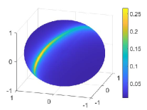
(a) Inter-event time function

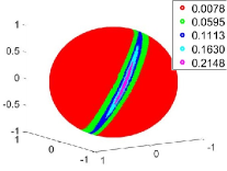
(b) State-space partitions

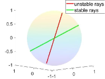
(c) Positively invariant rays

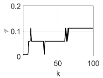
(d) Inter-event times evolution

Figure 1: Simulation results of Example 1.

Figure 1 presents the simulation results of Example 1. Figure 1(a) shows the value of the IET function $\tau_{e}(.)$ on the unit sphere under the relative thresholding event-triggering rule. The global minimum and global maximum of $\tau_{e}(.)$, respectively, are $\tau_{\min}=0.0088$ and $\tau_{\max}=0.2655$. We choose the number of regions $r=5$ and discretize the interval $[\tau_{\min},\tau_{\max}]$ into $5$ equal parts. Then, we partition the state space into $5$ regions and associate each region with the corresponding IET. Figure 1(b) shows the state-space partitions and the corresponding IET. In this case, the $G$ matrices corresponding to all the regions have real distinct positive eigenvalues. So, we can eliminate the possibility of existence of a PIS that does not contain a PIR. We can find numerically the four PIRs, which are shown in Figure 1(c). We can also analyze the stability of these PIRs by analyzing the spectrum of the corresponding $G$ matrices. Note that, here two of the PIRs are asymptotically stable and the other two are unstable. The two asymptotically stable PIRs form a positively invariant line passing through the origin and the point $(0.6813,-0.5616,0.4695)$. Similarly, the two unstable PIRs form a positively invariant line passing through the origin and the point $(0.1048,-0.3145,0.9435)$. Next, we choose an arbitrary vector close to one of the asymptotically stable PIRs as the initial state and Figure 1(d) presents the evolution of inter-event times under the RBSTR (3). We can see that the IETs converge to a steady state value which is exactly equal to the IET corresponding to one of the asymptotically stable PIRs.

Example 2

Next, let us consider a $5^{\text{th}}$ order system,

$$\dot{x}=\begin{bmatrix}0&1&0&0&0\\ 0&0&1&0&0\\ 0&0&0&1&0\\ 0&0&0&0&1\\ 30&-79&80&-40&10\end{bmatrix}x+\begin{bmatrix}0\\ 0\\ 0\\ 0\\ 1\end{bmatrix}u=:Ax+Bu.$$

The system matrix $A$ has eigenvalues at $\{1,2,3,2\pm i\}$. We choose the control gain $K$ so that $A_{c}:=A+BK$ has eigenvalues at $\{-0.1,-0.15,-0.2,-0.25,-0.3\}$. We first partition the state space into $50$ solid convex cones by using the recursive zonal equal area sphere partitioning toolbox [31, 32] in MATLAB which helps to partition higher dimensional unit spheres into regions of equal Lebesgue measure. Note that none of our results require the region-based self-triggered controller guarantee asymptotic stability of the equilibrium at the origin of the closed loop system. So, we arbitrarily assign an IET from the interval $[0.03,0.23]$ for each convex cone. As per Assumption (A1), if there are two convex cones with the same IET then they belong to the same region.

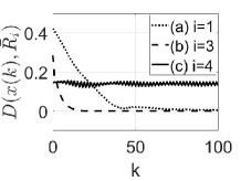
Figure 2: Simulation results of Example 2. (a) Asymptotically stable PIR ($\bar{R}_{1}$). (b) Asymptotically stable positively invariant radial line ($\bar{R}_{3}$). (c) Stable PIS which is a union of two rays ($\bar{R}_{4}$).

In this case, we identify the existence of four PISs $\bar{R}_{1},\bar{R}_{2},\bar{R}_{3}$ and $\bar{R}_{4}$. $\bar{R}_{1}$ and $\bar{R}_{2}$ are PIRs passing through the points $\begin{bmatrix}-0.8524&-0.4460&-0.2333&-0.1220&-0.0724\end{bmatrix}^{T}$ and $\begin{bmatrix}-1&-0.0003&0&0&0\end{bmatrix}^{T}$, respectively. $\bar{R}_{1}$ is a subset of a region with corresponding IET $0.2060$. Whereas $\bar{R}_{2}$ is a subset of a region with corresponding IET $0.0660$. $\bar{R}_{3}$ is a positively invariant radial line passing through the point $\begin{bmatrix}0&0&-0.0045&-0.0190&0.9998\end{bmatrix}^{T}$ in a region with corresponding IET $0.2260$. $\bar{R}_{3}$ is the eigensubspace corresponding to a real negative eigenvalue of the respective $G$ matrix. $\bar{R}_{4}$ is a union of two rays passing through the points $\begin{bmatrix}0.6241&0.3266&0.1737&0.1137&-0.6788\end{bmatrix}^{T}$ and $\begin{bmatrix}0.5831&0.3054&0.1574&0.0610&0.7336\end{bmatrix}^{T}$, respectively, in a region with corresponding IET $0.207385$. Note that, these two rays belong to the span of two eigenvectors of the respective $G$ matrix corresponding to two real distinct eigenvalues with magnitude equal to $\rho(G)$.

According to Theorem 9, we can analyze the stability of the intersection of these PISs with the unit sphere by studying the spectrum of the corresponding $G$ matrix. In this way, we see that both $\bar{R}_{1}\cap B_{1}(0)$ and $\bar{R}_{3}\cap B_{1}(0)$ are asymptotically stable. Whereas $\bar{R}_{2}\cap B_{1}(0)$ is unstable. Figure 2(a) and Figure 2(b), respectively, present the convergence of the system state to the asymptotically stable positively subregions $\bar{R}_{1}\cap B_{1}(0)$ and $\bar{R}_{3}\cap B_{1}(0)$ for an initial condition sufficiently close to the respective subregion. In Figure 2,

$$D(x(k),\bar{R}):=\text{dist}\left(\frac{x(k)}{\left\lVert x(k)\right\rVert},\ \bar{R}\cap B_{1}(0)\right)\vspace{-1ex}.$$

Note that $\bar{R}_{4}$ does not belong to the class of PISs considered in Theorem 9. But we can analyze the stability of $\bar{R}_{4}\cap B_{1}(0)$ in a similar way. In this case, the $G$ matrix corresponding to $\bar{R}_{4}$ is diagonalizable with $\sigma(G)=\{\lambda_{i}\}$, $i\in\{1,2,..,5\}$. We find that, $\lambda_{1}=-\lambda_{2}=\rho(G)$ and $|\lambda_{i}|<\rho(G)$ for all $i\in\{3,4,5\}$. Let $v_{i}$ denote an eigenvector of $G$ corresponding to an eigenvalue $\lambda_{i}$ for all $i\in\{1,2,..,5\}$. Note that $\bar{R}_{4}=\{\alpha u_{1}\cup\alpha u_{2}:\alpha\geq 0\}$ where $u_{1}=\alpha_{1}v_{1}+\alpha_{2}v_{2}$ and $u_{2}=\alpha_{1}v_{1}-\alpha_{2}v_{2}$ for some $\alpha_{1},\alpha_{2}\in$. As in the proof of Theorem 9, without loss of generality, let us suppose that $G$ and hence $J:=\frac{G}{\lambda_{1}}$ are in real Jordan form. Now, by using similar arguments as in the proof of Theorem 9, especially inequality (7) and the following discussion, we can show that $\bar{R}_{4}\cap B_{1}(0)$ is stable. Figure 2(c) presents the distance between $\bar{R}_{4}\cap B_{1}(0)$ and a $\gamma$ map for an initial condition arbitrarily close to $\bar{R}_{4}$.

V Conclusion

In this paper, we analyzed the evolution of IETs along the trajectories of linear systems under RBSTRs. Under this control method, studying steady state behavior of the IETs is equivalent to studying the existence of a conic subregion, which is a positively invariant set under the map that gives the evolution of the state from one event to the next. We provided necessary conditions and sufficient conditions for the existence of a PIS. We also provided necessary and sufficient conditions for a PIS to be stable and asymptotically stable. We extended this analysis to convergence of IETs to a given periodic sequence. We verified the proposed results through numerical simulations. Future work includes analysis of the average and periodicity of the IETs generated by a general class of triggering rules as well as the design of triggering policies under scheduling constraints.

References

- [1] P. Tabuada, “Event-triggered real-time scheduling of stabilizing control tasks,” IEEE Transactions on Automatic Control, vol. 52, no. 9, pp. 1680–1685, 2007.
- [2] W. Heemels, K. Johansson, and P. Tabuada, “An introduction to event-triggered and self-triggered control,” in 2012 IEEE 51st IEEE Conference on Decision and Control (CDC), 2012, pp. 3270–3285.
- [3] M. Lemmon, “Event-triggered feedback in control, estimation, and optimization,” in Networked control systems. Springer, 2010, pp. 293–358.
- [4] D. Tolić and S. Hirche, Networked control systems with intermittent feedback. CRC Press, 2017.
- [5] A. Anta and P. Tabuada, “To sample or not to sample: Self-triggered control for nonlinear systems,” IEEE Transactions on Automatic Control, vol. 55, no. 9, pp. 2030–2042, 2010.
- [6] W. P. M. H. Heemels, M. C. F. Donkers, and A. R. Teel, “Periodic event-triggered control for linear systems,” IEEE Transactions on Automatic Control, vol. 58, no. 4, pp. 847–861, 2013.
- [7] K. Astrom and B. Bernhardsson, “Comparison of Riemann and Lebesgue sampling for first order stochastic systems,” in Proceedings of the 41st IEEE Conference on Decision and Control, vol. 2, 2002, pp. 2011–2016.
- [8] B. Demirel, A. S. Leong, and D. E. Quevedo, “Performance analysis of event-triggered control systems with a probabilistic triggering mechanism: The scalar case,” 20th IFAC World Congress, vol. 50, no. 1, pp. 10 084–10 089, 2017.
- [9] F. D. Brunner, W. P. M. H. Heemels, and F. Allgower, “Robust event-triggered MPC with guaranteed asymptotic bound and average sampling rate,” IEEE Transactions on Automatic Control, vol. 62, no. 11, pp. 5694–5709, 2017.
- [10] P. Tallapragada, M. Franceschetti, and J. Cortés, “Event-triggered second-moment stabilization of linear systems under packet drops,” IEEE Transactions on Automatic Control, vol. 63, no. 8, pp. 2374–2388, 2018.
- [11] S. Bose and P. Tallapragada, “Event-triggered second moment stabilisation under action-dependent Markov packet drops,” IET Control Theory and Applications, vol. 15, no. 7, pp. 949–964, 2021.
- [12] P. Tallapragada and J. Cortés, “Event-triggered stabilization of linear systems under bounded bit rates,” IEEE Transactions on Automatic Control, vol. 61, no. 6, pp. 1575–1589, 2016.
- [13] Q. Ling, “Bit rate conditions to stabilize a continuous-time scalar linear system based on event triggering,” IEEE Transactions on Automatic Control, vol. 62, no. 8, pp. 4093–4100, 2017.
- [14] J. Pearson, J. P. Hespanha, and D. Liberzon, “Control with minimal cost-per-symbol encoding and quasi-optimality of event-based encoders,” IEEE Transactions on Automatic Control, vol. 62, no. 5, pp. 2286–2301, 2017.
- [15] M. J. Khojasteh, P. Tallapragada, J. Cortés, and M. Franceschetti, “The value of timing information in event-triggered control,” IEEE Transactions on Automatic Control, vol. 65, no. 3, pp. 925–940, 2020.
- [16] B. Asadi Khashooei, D. J. Antunes, and W. P. M. H. Heemels, “A consistent threshold-based policy for event-triggered control,” IEEE Control Systems Letters, vol. 2, no. 3, pp. 447–452, 2018.
- [17] F. D. Brunner, D. Antunes, and F. Allgower, “Stochastic thresholds in event-triggered control: A consistent policy for quadratic control,” Automatica, vol. 89, pp. 376 – 381, 2018.
- [18] M. Velasco, P. Martí, and E. Bini, “Equilibrium sampling interval sequences for event-driven controllers,” in European Control Conference (ECC), 2009, pp. 3773–3778.
- [19] R. Postoyan, R. G. Sanfelice, and W. Heemels, “Explaining the “mystery” of periodicity in inter-transmission times in two-dimensional event-triggered controlled system,” IEEE Transactions on Automatic Control, 2022.
- [20] A. Sharifi Kolarijani and M. Mazo, “Formal traffic characterization of lti event-triggered control systems,” IEEE Transactions on Control of Network Systems, vol. 5, no. 1, pp. 274–283, 2018.
- [21] G. Delimpaltadakis and M. Mazo, “Traffic abstractions of nonlinear homogeneous event-triggered control systems,” in 59th IEEE Conference on Decision and Control (CDC), 2020, pp. 4991–4998.
- [22] G. Delimpaltadakis, L. Laurenti, and M. Mazo, “Abstracting the sampling behaviour of stochastic linear periodic event-triggered control systems,” in 2021 60th IEEE Conference on Decision and Control (CDC), 2021, pp. 1287–1294.
- [23] G. de A. Gleizer and M. Mazo, “Computing the sampling performance of event-triggered control,” in Proceedings of the 24th International Conference on Hybrid Systems: Computation and Control, 2021.
- [24] G. de Albuquerque Gleizer and M. Mazo, “Computing the average inter-sample time of event-triggered control using quantitative automata,” Nonlinear Analysis: Hybrid Systems, vol. 47, p. 101290, 2023.
- [25] G. d. A. Gleizer and M. Mazo, “Chaos and order in event-triggered control,” IEEE Transactions on Automatic Control, pp. 1–16, 2023.
- [26] G. Delimpaltadakis and M. Mazo, “Isochronous partitions for region-based self-triggered control,” IEEE Transactions on Automatic Control, vol. 66, no. 3, pp. 1160–1173, 2021.
- [27] G. d. A. Gleizer, K. Madnani, and M. Mazo, “Self-triggered control for near-maximal average inter-sample time,” in 2021 60th IEEE Conference on Decision and Control (CDC), 2021, pp. 1308–1313.
- [28] A. Rajan and P. Tallapragada, “Analysis of inter-event times for planar linear systems under a general class of event triggering rules,” in 59th IEEE Conference on Decision and Control (CDC), 2020, pp. 5206–5211.
- [29] C. Fiter, L. Hetel, W. Perruquetti, and J.-P. Richard, “A state dependent sampling for linear state feedback,” Automatica, vol. 48, no. 8, pp. 1860–1867, 2012.
- [30] I. Gohberg, M. Kaashoek, and J. Kos, “The asymptotic behavior of the singular values of matrix powers and applications,” Linear Algebra and its Applications, vol. 245, pp. 55–76, 1996.
- [31] P. Leopardi, “Recursive zonal equal area sphere partitioning toolbox,” Matlab software package available via SourceForge: http://eqsp. sourceforge. net, 2005.
- [32] ——, “A partition of the unit sphere into regions of equal area and small diameter,” Electronic Transactions on Numerical Analysis, vol. 25, 01 2006.