Coupled three-mode squeezed vacuum: Gaussian steering and remote generation of Wigner negativity

Abstract

Multipartite Einstein-Podolsky-Rosen (EPR) steering and multimode quantum squeezing are essential resources for various quantum applications. The paper focuses on studying a coupled three-mode squeezed vacuum (C3MSV), which is a typical multimode squeezed Gaussian state and will exhibit peculiar steering property. Using the technique of integration within ordered products, we give the normal-ordering form for the coupled three-mode squeezing operator and derive the general analytical expressions of the statistical quantities for the C3MSV. Under Gaussian measurements, we analyze all bipartite Gaussian steerings (including no steering, one-way steering and two-way steering) in details and study the monogamy relations for the C3MSV. Then, we study the decoherence of all these steerings in noisy channels and find that sudden death will happen in a certain threshold time. Through the steerings shared in the C3MSV, we propose conceptual (and ideal) schemes of remotely generating Wigner negativity (WN) by performing appropriate photon subtraction(s) in the local position. Our obtained results may lay a solid theoretical foundation for a future practical study. We also believe that the C3MSV will be one of good candidate resources in future quantum protocols.

Keywords: Quantum correlation; Einstein-Podolsky-Rosen steering; quantum squeezing; decoherence; Wigner negativity

I Introduction

Quantum correlations have been intensively investigated in recent years and can manifest in different forms, such as entanglement, steering and Bell nonlocality 1 . These correlations are established in two-party, three-party, or even more-party systems and can be used as resources for quantum enhanced tasks 2 ; 3 ; 4 ; 5 . Entanglement is a striking feature of describing the nonbiseparability of states for two or more parties 6 . Bell nonlocality offers a vast research landscape with relevance for fundamental 7 and quantum technological applications 8 ; 9 . Eistein-Podolsky-Rosen (EPR) steering is intermediate between entanglement and Bell nonlocality 10 ; 11 ; 12 ; 13 ; 14 . Its concept was named by Schrodinger 15 and rigorously defined by Wiseman et al. 16 ; 17 . EPR steering is often the required resource enabling the protocol to proceed securely 18 and has been applied to realize different tasks 19 .

Over the past several decades, significant advances on squeezed light generation have been made 20 ; 21 . Squeezed optical fields, particularly those states with multimode squeezing, are essential resources in quantum technologies 22 . Nonlinear optics provides a number of promising experimental tools for realizing multipartite correlation and multimode squeezing 23 . One conventional tool is to employ the optical parametric oscillator technique 24 . Another mature tool is to employ a four-wave mixing (FWM) process 25 . FWM describes a parametric interaction between four coherent fields in a nonlinear crystal 26 .

There is a tendency for researchers to use multipartite quantum correlations and multimode quantum squeezing as resources. Specially, EPR steering in a multipartite scenario has been used for the implementation of secure multiuser quantum technologies 27 . Many schemes of generating multimode squeezed and correlated states have been proposed. Their common kernel idea is based on the basic FWM process by using multiple pump beams28 , spatially structured pump beams 29 ; 30 ; 31 or cascading setups 32 ; 33 ; 34 . These schemes of cascaded FWM processes can be used to generate 35 ; 36 ; 37 and even enhance 38 multipartite entanglement.

A two-mode squeezed vacuum (TMSV) is perhaps the most commonly used EPR entangled resource3 . Rather than a TMSV, many entangled resources (such as the NOON state 39 ; 40 and the Greenberger-Horne-Zeilinger state 41 ) have been also used in other scenarios. With the development and requirements of quantum technology, more and more entangled resources have been introduced and used42 ; 43 ; 44 ; 45 ; 46 . Based on the energy-level cascaded FWM system, Qin et al. constructed 11 possible Hamiltonians, which may help to generate three-mode and four-mode quantum squeezed states47 . Qin and co-worker generated triple-beam quantum-correlated states, which may show the tripartite entanglement34 . By FWM with linear and nonlinear beamsplitters, Liu et al. introduced a three-mode Gaussian state48 , which may exhibit tripartite EPR steering. Li et al. also generated quantum-correlated three-mode light beams49 . Zhang and Glasser50 introduced a coupled three-mode squeezed vacuum (C3MSV), which exhibits genuinely tripartite entanglement.

On the other hand, Wigner negativity (WN) 51 is arguably one of the most striking non-classical features of quantum states and has been attracting increasing interests 52 . Beyond its fundamental relevance 53 ; 54 , WN is also a necessary resource for quantum speedup with continuous variables. It has been seen as a necessary ingredient in continuous-variable quantum computation and simulation to outperform classical devices 55 ; 56 . As two important signatures of nonclassicality, quantum correlations can be intertwined with WN in the conditional generation of non-Gaussian states 57 ; 58 . Walschaers et al. developed a general formalism to prepare Wigner-negative states through EPR steering 59 ; 60 ; 61 . Xiang et al. proposed schemes for remote generation of WN through EPR steering in a multipartite scenario 62 , where they used a pure three-mode Gaussian state (realized by a feasible linear optical network) as the resource.

Intuitively, we think that the C3MSV will become an useful entangled resource in future quantum protocols. Except those properties such as squeezing and entanglement considered by Zhang and Glasser 50 , we will further study steering properties for the C3MSV in this paper. Considering the effect of the environment, we also study the decoherence of the steering. And then, we will propose schemes of remote preparation of Wigner negative states. One can refer to the appendixes for the derivation results and to the Supplemental Material 63 for the codes. The rest of the paper is structured as follows: In Sec.II, we make a brief introduction of the coupled three-mode squeezing operator (C3MSO) and the C3MSV. In Sec.III, we investigate the bipartite Gaussian steerings in the C3MSV. In Sec.IV, we study the decoherence of the steering. In Sec.V, we propose schemes to remotely generate WN based on the steering in the C3MSV. Conclusions are summarized in the last section.

II Coupled three-mode squeezed vacuum

An interaction with the three-mode Hamiltonian $H_{I}=i\hbar(\eta_{1}^{\ast}a_{1}a_{2}$ $+\eta_{2}^{\ast}a_{2}a_{3}$ $-\eta_{1}a_{1}^{\dagger}a_{2}^{\dagger}$ $-\eta_{2}a_{2}^{\dagger}a_{3}^{\dagger})$ can be realized by using a dual-pumping FWM process, where $a_{j}$ ($a_{j}^{\dagger}$) is the bosonic annihilation (creation) operator in mode $j$. The detailed description of the interaction has been provided by Zhang and Glasser 50 . Associated with this Hamiltonian, one can obtain the following unitary time evolution operator (i.e., the C3MSO)

$$S_{3}=e^{\xi_{1}^{\ast}a_{1}a_{2}+\xi_{2}^{\ast}a_{2}a_{3}-\xi_{1}a_{1}^{\dagger}a_{2}^{\dagger}-\xi_{2}a_{2}^{\dagger}a_{3}^{\dagger}},$$ (1)

where $\xi_{j}=\eta_{j}t=r_{j}e^{i\theta_{j}}$ ($j=1$ and $2$) are the two complex squeezing parameters, with respective magnitude $r_{j}$ and phase $\theta_{j}$. It is obvious to see $S_{3}^{-1}=S_{3}^{{\dagger}}$. For convenience, we reset ($r_{1}$, $r_{2}$) as ($r$, $\phi$), satisfying $r=\sqrt{r_{1}^{2}+r_{2}^{2}}$, $\cos\phi=r_{1}/r$, and $\sin\phi=r_{2}/r$ with $\phi\in[0,\pi/2]$ [see Fig.1(a)]. A similar three-mode squeezing interaction has also been analyzed theoretically and realized experimentally by Paris’s group. By interlinked nonlinear interactions in $\chi^{(2)}$ media, they addressed the generation of fully inseparable three-mode entangled states of radiation 64 ; 65 . In addition, they applied this three-mode entanglement in realizing symmetric and asymmetric telecloning machines and generalized these studies to multimode cases 66 .

As illustrated in Fig.1(b), by applying the C3MSO $S_{3}$ on the three independent vacuum $\left|0\right\rangle\left|0\right\rangle\left|0\right\rangle$, we easily obtain the C3MSV with the following form

$$\left|\psi\right\rangle\equiv S_{3}\left|000\right\rangle=\frac{1}{c}e^{-\frac{\epsilon_{1}}{c}a_{1}^{{\dagger}}a_{2}^{{\dagger}}-\frac{\epsilon_{2}}{c}a_{2}^{{\dagger}}a_{3}^{{\dagger}}}\left|000\right\rangle,$$ (2)

whose density operator is $\rho_{123}=\left|\psi\right\rangle\left\langle\psi\right|$. In Appendix A, we have given the normal-ordering form for the C3MSO by using the technique of integration within ordered products (IWOP) 67 ; 68 . Here, we set $c=\cosh r$, $s=\sinh r$, $\epsilon_{1}=se^{i\theta_{1}}\cos\phi$, and $\epsilon_{2}=se^{i\theta_{2}}\sin\phi$. In particular, if $\xi_{2}=0,$ then $\left|\psi\right\rangle=S_{2}(\xi_{1})\left|00\right\rangle_{12}\otimes\left|0\right\rangle_{3}$; if $\xi_{1}=0,$ then $\left|\psi\right\rangle=\left|0\right\rangle_{1}\otimes S_{2}(\xi_{2})\left|00\right\rangle_{23}$, with $S_{2}(\xi_{1})=e^{\xi_{1}^{\ast}a_{1}a_{2}-\xi_{1}a_{1}^{\dagger}a_{2}^{\dagger}}$ and $S_{2}(\xi_{2})=e^{\xi_{2}^{\ast}a_{2}a_{3}-\xi_{2}a_{2}^{\dagger}a_{3}^{\dagger}}$. Moreover, if $\xi_{1}=\xi_{2}$ (i.e. $\phi=\pi/4$), the C3MSV is a bisymmetric state, whose mode 1 and mode 3 are symmetrical with mode 2. Zhang and Glasser have analyzed the squeezing property and the entanglement characteristics for the C3MSV50 , which further reflect that the C3MSO has the utility of realizing available squeezing and genuine tripartite entanglement.

Using the general expression for the C3MSV in Eq.(A4), we easily obtain $\bar{n}_{1}=s^{2}\cos^{2}\phi$, $\bar{n}_{2}=s^{2}$, $\bar{n}_{3}=s^{2}\sin^{2}\phi$, and $\bar{n}_{T}=2s^{2}$, i.e., the mean photon numbers (MPNs) for mode 1, mode 2, mode 3 and total modes, respectively [see Fig.1(c)]. By the way, we often replace $r$ by $\bar{n}_{T}$ (using $r=$arcsinh$\sqrt{\bar{n}_{T}/2}$) and set $\theta_{1}=\theta_{2}=0$ in our following numerical work.

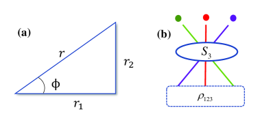
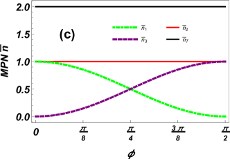
Figure 1: (a) ($r_{1}$, $r_{2}$) are reset to ($r$, $\phi$). (b) Conceptual generating scheme of the C3MSV $\rho_{123}$, which is obtained by applying $S_{3}$ on three independent vacuums $\left|000\right\rangle$ (represented by three small balls separately at the top). (c) MPNs $\bar{n}_{1}$, $\bar{n}_{2}$, $\bar{n}_{3}$, and $\bar{n}_{T}$ versus $\phi$ (setting $\bar{n}_{T}=2$).

III Gaussian steering in the C3MSV

The C3MSV is a pure three-mode entangled Gaussian state, which can be seen from its Wigner function provided in Eq. (C1). In this section, we analyze the distributions of bipartite Gaussian steerings in the C3MSV, without considering the optical losses and thermal noises.

III.1 Covariance matrix of the C3MSV

The covariance matrix (CM) 69 ; 70 ; 71 ; 72 ; 73 of the C3MSV is expressed as

$$V=\left(\begin{array}[]{ccc}(1+2\bar{n}_{1})\text{ }1_{2}&-2sc\cos\phi\text{ }\Sigma_{\theta_{1}}&s^{2}\sin 2\phi\text{ }R_{\theta_{2}-\theta_{1}}\\ -2sc\cos\phi\text{ }\Sigma_{\theta_{1}}&(1+2\bar{n}_{2})\text{ }1_{2}&-2sc\sin\phi\text{ }\Sigma_{\theta_{2}}\\ s^{2}\sin 2\phi\text{ }\tilde{R}_{\theta_{2}-\theta_{1}}&-2sc\sin\phi\text{ }\Sigma_{\theta_{2}}&(1+2\bar{n}_{3})\text{ }1_{2}\end{array}\right),$$ (3)

with the $2\times 2$ identity matrix $1_{2}$ and

$$\Sigma_{\theta}=\left(\begin{array}[]{cc}\cos\theta&\sin\theta\\ \sin\theta&-\cos\theta\end{array}\right),R_{\theta}=\left(\begin{array}[]{cc}\cos\theta&\sin\theta\\ -\sin\theta&\cos\theta\end{array}\right).$$ (4)

The matrix elements of the CM, defined by $V_{jk}=\left\langle\psi\right|(\hat{X}_{j}\hat{X}_{k}+\hat{X}_{k}\hat{X}_{j})\left|\psi\right\rangle$, are expressed via the vector $\hat{X}=(\hat{x}_{1},\hat{p}_{1},\hat{x}_{2},\hat{p}_{2},\hat{x}_{3},\hat{p}_{3}$). For each mode, we define the position operator $\hat{x}_{j}=\frac{1}{\sqrt{2}}(\hat{a}_{j}+\hat{a}_{j}^{{\dagger}})$ and the momentum operator $\hat{p}_{j}=\frac{1}{i\sqrt{2}}(\hat{a}_{j}-\hat{a}_{j}^{{\dagger}})$, accompanied by its annihilation and creation operators $\hat{a}_{j}$ and $\hat{a}_{j}^{{\dagger}}$. It is noted that $\left\langle\hat{x}_{j}\right\rangle=\left\langle\hat{p}_{j}\right\rangle=0$ for each mode of the C3MSV. The CM $V$ in Eq.(3) is a symmetric and positive semidefinite matrix (with eigenvalues $1$, $1$, $e^{-2r}$, $e^{-2r}$, $e^{2r}$, and $e^{2r}$) and obeys $V+i\Omega^{\oplus 3}\geq 0$ with $\Omega=\left(\begin{array}[]{cc}0&1\\ -1&0\end{array}\right)$. Moreover, we can check $\det V=1$ and prove that the C3MSV is a pure state.

III.2 Bipartite Gaussian steering

Quantum protocols often require only states (e.g., squeezed vacuum states) and measurements (e.g., homodyne detection) that are simple to realize on quantum optics platforms. Undoubtedly, the C3MSV is a good candidate Gaussian state. Meanwhile, one can explore the Gaussian steerings by Gaussian measurements 74 ; 75 . Moreover, the distribution of the steering can be constrained by its monogamy relation. Reid derived monogamy inequalities for the bipartite EPR steering distributed among different systems 76 . Xiang et al. derived the laws for the distribution of quantum steering among different parties and proved a monogamy relation of Gaussian steering 77 .

The CM of a bipartite Gaussian state can be expressed as

$$\sigma_{AB}=\left(\begin{array}[]{cc}V_{A}&V_{AB}\\ V_{AB}^{T}&V_{B}\end{array}\right),$$ (5)

where party $A$ and party $B$ are the bipartite subsystems. Then, we can quantify how much it is steerable via the following quantity

$$\mathcal{G}^{A\rightarrow B}\left(V\right):=\max\{0,-\sum_{j:\text{ }\bar{\nu}_{j}^{B|A}<1}\ln\bar{\nu}_{j}^{B|A}\}.$$ (6)

where $\{\bar{\nu}_{j}^{B|A}\}_{j=1}^{2n_{B}}$ denote the symplectic eigenvalues ($n_{B}$ is the mode number in subsystem $B$) of the Schur complement $\sigma_{B|A}=V_{B}-V_{AB}^{T}V_{A}^{-1}V_{AB}$ of $\sigma_{AB}$. Obviously, the mathematical formalism of Gaussian steering $\mathcal{G}^{A\rightarrow B}$ is achieved by Gaussian measurements in party $A$. This quantity $\mathcal{G}^{A\rightarrow B}$ is defined as Gaussian $A\rightarrow B$ steerability, which is a monotone under Gaussian local operations and classical communication. Moreover, the larger $\mathcal{G}^{A\rightarrow B}$ is, the stronger Gaussian steerability is 10 ; 78 .

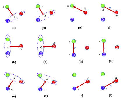
Figure 2: Bipartite assignments in the C3MSV, where $A$ is the steering party and $B$ is the steered party.

In what follows, we take party $A$ and party $B$ from the three modes of the C3MSV and construct 12 kinds of $\sigma_{AB}$s from $V$ in Eq. (3). The steering party $A$ and the steered party $B$ are assigned as shown in Fig.2. According to the rule in Eq. (6), we obtain the following steerings present in the C3MSV.

Case (a)$\Longrightarrow$A(23)-B(1). In this case, we have $\bar{\nu}_{1}^{B|A}=\bar{\nu}_{2}^{B|A}=(c^{2}+s^{2}\cos 2\phi)^{-1}<1$, which leads to

$$\mathcal{G}^{23\rightarrow 1}=2\ln(c^{2}+s^{2}\cos 2\phi).$$ (7)

Case (b)$\Longrightarrow$A(13)-B(2). In this case, we have $\bar{\nu}_{1}^{B|A}=\bar{\nu}_{2}^{B|A}=(c^{2}+s^{2})^{-1}<1$, which leads to

$$\mathcal{G}^{13\rightarrow 2}=2\ln(c^{2}+s^{2}).$$ (8)

Case (c)$\Longrightarrow$A(12)-B(3). In this case, we have $\bar{\nu}_{1}^{B|A}=\bar{\nu}_{2}^{B|A}=(c^{2}-s^{2}\cos 2\phi)^{-1}<1$, which leads to

$$\mathcal{G}^{12\rightarrow 3}=2\ln(c^{2}-s^{2}\cos 2\phi).$$ (9)

Case (d)$\Longrightarrow$A(1)-B(23). In this case, we have $\bar{\nu}_{1}^{B|A}=\bar{\nu}_{2}^{B|A}=\left(\varkappa_{1}-\sqrt{\varkappa_{2}}\right)/\varkappa_{0}<1$ and $\bar{\nu}_{3}^{B|A}=\bar{\nu}_{4}^{B|A}=\left(\varkappa_{1}+\sqrt{\varkappa_{2}}\right)/\varkappa_{0}\geq 1$, which leads to

$$\mathcal{G}^{1\rightarrow 23}=2\ln[\varkappa_{0}/\left(\varkappa_{1}-\sqrt{\varkappa_{2}}\right)],$$ (10)

with

$$\varkappa_{0} = 4+8s^{2}\cos^{2}\phi,$$

$$\varkappa_{1} = 1+3c^{2}+\left(3-2\cos 2\phi\right)s^{2},$$

$$\varkappa_{2} = \left(19-12\cos 2\phi\right)c^{2}s^{2}$$ (11)

$$+\left(19-12\cos 2\phi+2\cos 4\phi\right)s^{4}$$

$$+\left(13-20\cos 2\phi\right)s^{2}.$$

Case (e)$\Longrightarrow$A(2)-B(13). In this case, we have $\bar{\nu}_{1}^{B|A}=\bar{\nu}_{2}^{B|A}=(c^{2}+s^{2})^{-1}<1$ and $\bar{\nu}_{3}^{B|A}=\bar{\nu}_{4}^{B|A}=1$, which leads to

$$\mathcal{G}^{2\rightarrow 13}=2\ln(c^{2}+s^{2}).$$ (12)

Case (f)$\Longrightarrow$A(3)-B(12). In this case, we have $\bar{\nu}_{1}^{B|A}=\bar{\nu}_{2}^{B|A}=\left(\iota_{1}-\sqrt{\iota_{2}}\right)/\iota_{0}<1$ and $\bar{\nu}_{3}^{B|A}=\bar{\nu}_{4}^{B|A}=\left(\iota_{1}+\sqrt{\iota_{2}}\right)/\iota_{0}\geq 1$, which leads to

$$\mathcal{G}^{3\rightarrow 12}=2\ln[\iota_{0}/\left(\iota_{1}-\sqrt{\iota_{2}}\right)],$$ (13)

with

$$\iota_{0} = 4+8s^{2}\sin^{2}\phi,$$

$$\iota_{1} = 1+3c^{2}+(3+2\cos 2\phi)s^{2},$$

$$\iota_{2} = \left(19+12\cos 2\phi\right)c^{2}s^{2}+$$ (14)

$$\left(19+12\cos 2\phi+2\cos 4\phi\right)s^{4}$$

$$+\left(13+20\cos 2\phi\right)s^{2}.$$

Case (g)$\Longrightarrow$A(2)-B(1). In this case, we have $\bar{\nu}_{1}^{B|A}=\bar{\nu}_{2}^{B|A}=(c^{2}-s^{2}\cos 2\phi)/(c^{2}+s^{2})<1$, which leads to

$$\mathcal{G}^{2\rightarrow 1}=2\ln[(c^{2}+s^{2})/(c^{2}-s^{2}\cos 2\phi)].$$ (15)

Case (h)$\Longrightarrow$A(1)-B(3). In this case, we have $\bar{\nu}_{1}^{B|A}=\bar{\nu}_{2}^{B|A}=(c^{2}+s^{2})/(1+2s^{2}\cos^{2}\phi)\geq 1$,, which leads to

$$\mathcal{G}^{1\rightarrow 3}=0.$$ (16)

Case (i)$\Longrightarrow$A(2)-B(3). In this case, we have $\bar{\nu}_{1}^{B|A}=\bar{\nu}_{2}^{B|A}=(c^{2}+s^{2}\cos 2\phi)/(c^{2}+s^{2})<1$, which leads to

$$\mathcal{G}^{2\rightarrow 3}=2\ln[(c^{2}+s^{2})/(c^{2}+s^{2}\cos 2\phi)].$$ (17)

Case (j)$\Longrightarrow$A(1)-B(2). In this case, we have $\bar{\nu}_{1}^{B|A}=\bar{\nu}_{2}^{B|A}=(c^{2}-s^{2}\cos 2\phi)/(1+2s^{2}\cos^{2}\phi)\geq 1$, which leads to

$$\mathcal{G}^{1\rightarrow 2}=0.$$ (18)

Case (k)$\Longrightarrow$A(3)-B(1). In this case, we have $\bar{\nu}_{1}^{B|A}=\bar{\nu}_{2}^{B|A}=(c^{2}+s^{2})/(1+2s^{2}\sin^{2}\phi)\geq 1$, which leads to

$$\mathcal{G}^{3\rightarrow 1}=0.$$ (19)

Case (l)$\Longrightarrow$A(3)-B(2). In this case, we have $\bar{\nu}_{1}^{B|A}=\bar{\nu}_{2}^{B|A}=(c^{2}+s^{2}\cos 2\phi)/(1+2s^{2}\sin^{2}\phi)\geq 1$, which leads to

$$\mathcal{G}^{3\rightarrow 2}=0.$$ (20)

More interestingly, all the above steerings are independent of phases ($\theta_{1}$, $\theta_{2}$). As we all know, EPR steering is a directional form of nonlocality and possesses an asymmetric property. This characteristic can also be reflected in our steerings. In Fig.3, we draw the contour plots of $\mathcal{G}^{12\rightarrow 3}$, $\mathcal{G}^{1\rightarrow 23}$, $\mathcal{G}^{23\rightarrow 1}$, $\mathcal{G}^{3\rightarrow 12}$, $\mathcal{G}^{2\rightarrow 1}$, and $\mathcal{G}^{2\rightarrow 3}$ in the ($\bar{n}_{T}$, $\phi$) space. Interestingly, $\mathcal{G}^{12\rightarrow 3}$ with $\mathcal{G}^{1\rightarrow 23}$, $\mathcal{G}^{23\rightarrow 1}$ with $\mathcal{G}^{3\rightarrow 12}$, and $\mathcal{G}^{2\rightarrow 1}$ with $\mathcal{G}^{2\rightarrow 3}$, all have the symmetry on the axis $\phi=\pi/4$. This is due to self-characteristics of the C3MSV. In Fig.4, we plot $\mathcal{G}^{A\rightarrow B}$s versus $\phi$ (with $\bar{n}_{T}=3$) and $\mathcal{G}^{A\rightarrow B}$s versus $\bar{n}_{T}$ (with $\phi=\pi/8$). Among them, $\mathcal{G}^{13\rightarrow 2}=\mathcal{G}^{2\rightarrow 13}$ are functions of $\bar{n}_{T}$ and are not independent of $\phi$. Moreover, we know that $\mathcal{G}^{1\rightarrow 2}=\mathcal{G}^{1\rightarrow 3}=\mathcal{G}^{3\rightarrow 1}=\mathcal{G}^{3\rightarrow 2}=0$, but $\mathcal{G}^{2\rightarrow 1}>0$ (except $\phi=\pi/2$), $\mathcal{G}^{2\rightarrow 3}>0$ (except $\phi=0$), and $\mathcal{G}^{2\rightarrow 1}=\mathcal{G}^{2\rightarrow 3}$ for $\phi=\pi/4$. As $\bar{n}_{T}$ increasing, most of the $\mathcal{G}^{A\rightarrow B}$s will increase. The results tell us that three types of steerings, i.e., no steering ($A$ cannot steer $B$ and $B$ cannot steer $A$), one-way steering ($A$ can steer $B$ while $B$ cannot steer $A$), or two-way (symmetrical or asymmetrical) steering ($A$ can steer $B$ and $B$ can steer $A$), are presented in the C3MSV. The main results are summarized as follows.

(i) There is no steering between mode 1 and mode 3 because of $\mathcal{G}^{1\rightarrow 3}=0$ and $\mathcal{G}^{3\rightarrow 1}=0$ [see Eq.(16) and Eq.(19)].

(ii) There is one-way steering between mode 1 and mode 2 because of $\mathcal{G}^{2\rightarrow 1}>0$ and $\mathcal{G}^{1\rightarrow 2}=0$ [see Eq.(15) and Eq.(18)].

(iii) There is one-way steering between mode 2 and mode 3 because of $\mathcal{G}^{2\rightarrow 3}>0$ and $\mathcal{G}^{3\rightarrow 2}=0$ [see Eq.(17) and Eq.(20)].

(iv) There is two-way asymmetrical steering between mode 1 and group (23) because of $\mathcal{G}^{23\rightarrow 1}>0$ and $\mathcal{G}^{1\rightarrow 23}>0$ but $\mathcal{G}^{23\rightarrow 1}\neq\mathcal{G}^{1\rightarrow 23}$ [see Eq.(7) and Eq.(10)].

(v) There is two-way symmetrical steering between mode 2 and group (13) because of $\mathcal{G}^{13\rightarrow 2}=$ $\mathcal{G}^{2\rightarrow 13}>0$ [see Eq.(8) and Eq.(12)].

(vi) There is two-way asymmetrical steering between mode 3 and group (12) because of $\mathcal{G}^{12\rightarrow 3}>0$ and $\mathcal{G}^{3\rightarrow 12}>0$ but $\mathcal{G}^{12\rightarrow 3}\neq\mathcal{G}^{3\rightarrow 12}$ [see Eq.(9) and Eq.(13)].

Just like what He et al. said in their work14 , our results also show that each mode can be steered by one or both of the other two in the C3MSV. Moreover, we find that (a) $\mathcal{G}^{2\rightarrow 1}>0$, but $\mathcal{G}^{3\rightarrow 1}=0$, and (b) $\mathcal{G}^{2\rightarrow 3}>0$, but $\mathcal{G}^{1\rightarrow 3}=0$. This result holds the character that two parties cannot steer the same system 76 .

Figure 3: (a) $\mathcal{G}^{12\rightarrow 3}$, (b) $\mathcal{G}^{23\rightarrow 1}$, (c) $\mathcal{G}^{1\rightarrow 23}$, (d) $\mathcal{G}^{3\rightarrow 12}$, (e) $\mathcal{G}^{2\rightarrow 1}$, and (f) $\mathcal{G}^{2\rightarrow 3}$ as functions of $\bar{n}_{T}$ and $\phi$.

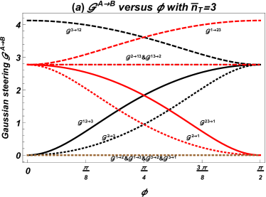
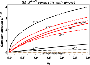
Figure 4: (a) $\mathcal{G}^{A\rightarrow B}$ versus $\phi$ (setting $\bar{n}_{T}=3$). (b) $\mathcal{G}^{A\rightarrow B}$ versus $\bar{n}_{T}$ (setting $\phi=\pi/8$).

III.3 Monogamy relations

Monogamy means that two observers cannot simultaneously steer the state of the third party. Both theoretical and experimental results show the monogamous relation in multipartite EPR steering 79 . In 2017, Xiang et al. defined the concept of the residual Gaussian steering (RGS) 77 . Here, we use the RGS to quantify the genuine tripartite steering for the C3MSV. Using all the above expressions from Eqs.(7) to (20), we check that the following monogamy relations

$$\mathcal{G}^{\left(23\right)\rightarrow 1}-\mathcal{G}^{2\rightarrow 1}-\mathcal{G}^{3\rightarrow 1} \geq 0,$$

$$\mathcal{G}^{\left(31\right)\rightarrow 2}-\mathcal{G}^{3\rightarrow 2}-\mathcal{G}^{1\rightarrow 2} \geq 0,$$

$$\mathcal{G}^{\left(12\right)\rightarrow 3}-\mathcal{G}^{1\rightarrow 3}-\mathcal{G}^{2\rightarrow 3} \geq 0,$$ (21)

and

$$\mathcal{G}^{1\rightarrow\left(23\right)}-\mathcal{G}^{1\rightarrow 2}-\mathcal{G}^{1\rightarrow 3} \geq 0,$$

$$\mathcal{G}^{2\rightarrow\left(31\right)}-\mathcal{G}^{2\rightarrow 3}-\mathcal{G}^{2\rightarrow 1} \geq 0,$$

$$\mathcal{G}^{3\rightarrow\left(12\right)}-\mathcal{G}^{3\rightarrow 1}-\mathcal{G}^{3\rightarrow 2} \geq 0,$$ (22)

hold for the C3MSV. Further, we consider the RGS

$$\mathcal{G}^{1:2:3} = \min_{\left\langle i,j,k\right\rangle}\{\mathcal{G}^{\left(jk\right)\rightarrow i}-\mathcal{G}^{j\rightarrow i}-\mathcal{G}^{k\rightarrow i}\}$$ (23)

$$= \min_{\left\langle i,j,k\right\rangle}\{\mathcal{G}^{i\rightarrow\left(jk\right)}-\mathcal{G}^{i\rightarrow j}-\mathcal{G}^{i\rightarrow k}\},$$

for the C3MSV, where $\left\langle i,j,k\right\rangle$ denotes any cycle permutation of $1$, $2$, and $3$. In Fig.5(a) we plot the RGS as a function of $\bar{n}_{T}$ and $\phi$. From which, we see that the RGS is maximized on bisymmetric C3MSV with $\phi=\pi/4$, i.e., $r_{1}=r_{2}$. In this case, the genuine tripartite $\mathcal{G}^{1:2:3}$ reduces to the collective steering $\mathcal{G}^{13\rightarrow 2}=\mathcal{G}^{2\rightarrow 13}=2\ln(c^{2}+s^{2})$. Figure 5(b) presents the RGS as a function of $\phi$ with different $\bar{n}_{T}$, which are the sections of Fig.5(a). Indeed, the RGS acts as an indicator of collective steering-type correlations.

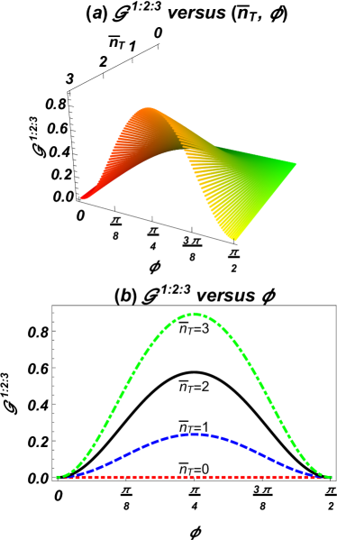
Figure 5: RGS $\mathcal{G}^{1:2:3}$ for the C3MSV with CM $V$ (a) in the ($\bar{n}_{T}$, $\phi$) space and (b) versus $\phi$ with different $\bar{n}_{T}$.

IV Decoherence of steering for the C3MSV

When dealing in a practical application, detector efficiencies and real world effects such as losses and electronic noise will arise and become crucial in a real experimental demonstration. Especially in the quantum realm, decoherence properties will dominate. Following the handling ways of Reid’s group 80 and Paris’s group 66 ; 81 ; 82 , we study the decoherence of the steering for the C3MSV in this section. As shown in Fig.6, we consider the evolution of the C3MSV in three independent noisy channels (characterized by the loss rates $\gamma_{j}$ and the thermal photons $\bar{n}_{R_{j}}$). The solution in mode $j$ is straightforward to evaluate by using the operator Langevin equation 83 ; 84

$$\dot{a}_{j}=-\gamma_{j}a_{j}+\sqrt{2\gamma_{j}}\Gamma_{j},$$ (24)

which describe the evolution of the mode operator $a_{j}$. Here, the annihilation operator $\Gamma_{j}$ describes the thermal reservoir $j$ with the occupation number $\bar{n}_{R_{j}}$ and the factor $\gamma_{j}$ of mode $j$ describes the decay (loss) rate that is induced by its reservoir.

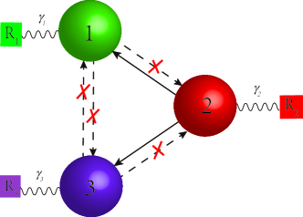
Figure 6: Each mode (mode $j$) in the C3MSV is independently coupled to its respective reservoir $R_{j}$ parametrized by the loss rate $\gamma_{j}$. These three couplings induce the decoherence of the steerings of the C3MSV.

Using the results provided in Appendix B, we can obtain the CM at time $t$ as follows

$$V\left(t\right)=\left(\begin{array}[]{ccc}\mathcal{A}_{1}\text{ }1_{2}&\mathcal{B}_{1}\text{ }\Sigma_{\theta_{1}}&\mathcal{B}_{3}\text{ }R_{\theta_{2}-\theta_{1}}\\ \mathcal{B}_{1}\text{ }\Sigma_{\theta_{1}}&\mathcal{A}_{2}\text{ }1_{2}&\mathcal{B}_{2}\text{ }\Sigma_{\theta_{2}}\\ \text{ }\mathcal{B}_{3}\text{ }\tilde{R}_{\theta_{2}-\theta_{1}}&\text{ }\mathcal{B}_{2}\Sigma_{\theta_{2}}&\mathcal{A}_{3}\text{ }1_{2}\end{array}\right),$$ (25)

with $\mathcal{A}_{j}=1+2\bar{n}_{j}+2\bar{n}_{R_{j}}(1-e^{-2\gamma_{j}t})$, $\mathcal{B}_{1}=-2sce^{-(\gamma_{1}+\gamma_{2})t}\cos\phi$, $\mathcal{B}_{2}=-2sce^{-(\gamma_{2}+\gamma_{3})t}\sin\phi$, and $\mathcal{B}_{3}=s^{2}e^{-(\gamma_{1}+\gamma_{3})t}\sin 2\phi$. Equation (25) with $t=0$ can be reduced to Eq.(3) as expected. Based on the CM in Eq.(25) and using the aforementioned steering criterion, we can analyze the evolution of the steering.

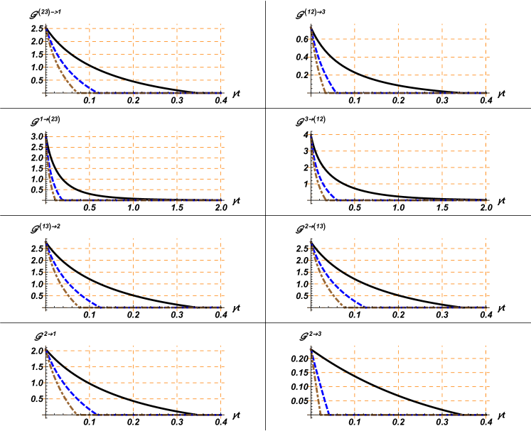
Figure 7: Decoherence of several steerings of the C3MSV with $\bar{n}_{T}=3$ and $\phi=\pi/8$ and in different environments. $\mathcal{G}^{A\rightarrow B}$ versus $\gamma t$ in different $\bar{n}_{R}$. The solid black line refers to the case $\bar{n}_{R}=0$. The dashed blue line refers to the case $\bar{n}_{R}=0.5$. The dotdashed brown line refers to the case $\bar{n}_{R}=1$. For each case, the sudden death will be observed at a threshold time.

Quite obviously, the dynamics of the steering is very complex because the interaction is related with many parameters, including $r$, $\phi$, $\theta_{1}$, $\theta_{2}$, $\gamma_{1}$, $\gamma_{2}$, $\gamma_{3}$, $\bar{n}_{R_{1}}$, $\bar{n}_{R_{2}}$, $\bar{n}_{R_{3}}$, and $t$. In fact, EPR steering may be adjusted by varying the noise on different parties of the C3MSV. Similar works on manipulating the direction 85 or the dynamics (such as death or revival) 86 of EPR steering have been demonstrated. Without loss of generality, we only set $\gamma_{1}=\gamma_{2}=\gamma_{3}=\gamma$ and $\bar{n}_{R_{1}}=\bar{n}_{R_{2}}=\bar{n}_{R_{3}}=\bar{n}_{R}$. Using the C3MSV with $\bar{n}_{T}=3$ and $\phi=\pi/8$ and the environments with $\bar{n}_{R}=0$, $0.5$, and $1$ as an example, we depict the evolution of several steerings in Fig.7. These results show that: (i) The steerability will decrease as time $\gamma t$ increases, and (ii) Until $\gamma t$ exceeds a certain threshold value, sudden death is observed. Moreover, the threshold time is shorten by increasing $\bar{n}_{R}$. Taking $\mathcal{G}^{23\rightarrow 1}$ of Fig.7 as an example, the sudden deaths are observed at $\gamma t$ $=$ $0.346574$, $0.11903$, and $0.0729227$, for $\bar{n}_{R}=0$, $0.5$, and $1$, respectively.

V Protocols of preparing Wigner negativity remotely

As Walschaers et al. recently pointed out, when party $A$ and party $B$ share a Gaussian state, party $B$ can perform some measurement on itself to create Wigner negativity on party $A$, if and only if there is a Gaussian steering from party $A$ to party $B$ 57 . Moreover, they provided an intuitive method to quantify remotely generated WN by employing non-Gaussian operation of photon subtraction. Following methods in Walschaers’ work 59 and Xiang’s work 62 , we investigate the remote creation and distribution of WN in the tripartite C3MSV. Here, we declare that we only study ideal and conceptual protocols of preparing WN, without considering any lossy channels. Based on the C3MSV, we keep the steered party $B$ in the local station and send the steering party $A$ to the remote position. After appropriate single-photon subtraction(s) on the steered party $B$, the steering party $A$ becomes a reduced non-Gaussian state $\rho_{B_{a}|A}$. In some cases, we can generate Wigner negative states in the remote position. For state $\rho_{j}$, we can derive its Wigner function (WF) by $W_{\rho_{j}}\left(\beta_{j}\right)=\mathrm{Tr}(\hat{O}_{w_{j}}\rho_{j})$, with $\hat{O}_{w_{j}}=\frac{2}{\pi}:e^{-2(\hat{a}_{j}^{{\dagger}}-\beta_{j}^{\ast})(\hat{a}_{j}-\beta_{j})}:$ ($:\cdots:$ denotes the normal ordering) and $\beta_{j}=\left(x_{j}+iy_{j}\right)/\sqrt{2}$87 ; 88 . Furthermore, we can quantify the WN of $\rho_{B_{a}|A}$ as

$$\mathcal{N}\equiv\int\left|W(\beta)\right|d^{2n_{A}}\beta-1,$$ (26)

with $\beta\in\mathbb{R}^{2n_{A}}$, where $n_{A}$ is the mode number considered in party $A$. As shown schematically in Fig.8, we propose protocols of generating 18 kinds of $\rho_{B_{a}|A}$s, whose analytical WFs are given in Appendix C. As examples, we plot WFs for $\rho_{B_{a}|A}$s with $\bar{n}_{T}=3$ and $\phi=\pi/8$ in Fig.9, where only several WFs exhibits the WNs.

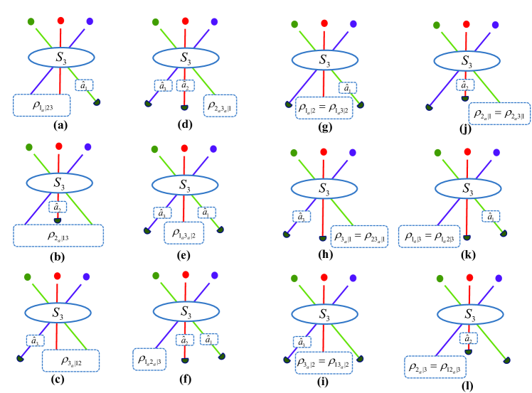
Figure 8: Ideal and conceptual schemes of remote generated non-Gaussian states $\rho_{B_{a}|A}$ based on the C3MSV, without considering the loss in any channel. Note that cases (a)-(c) are two-mode states and cases (d)-(l) are one-mode states.

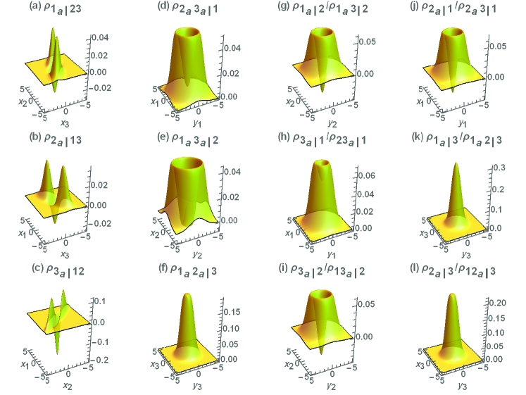
Figure 9: WFs of $\rho_{B_{a}|A}$s corresponding to Fig.8, with $\bar{n}_{T}=3$, $\phi=\pi/8$, and $\theta_{1}=\theta_{2}=0$. Some cases have WNs and some cases have no WNs.

Indeed, the amount of WN cannot be freely distributed among different modes. It can be influenced by the considered protocols and the interaction parameters. In order to explain the characters, we plot some WNs $\mathcal{N}$ versus $\phi$ by fixing $\bar{n}_{T}=3$ in Fig.10 and versus $\bar{n}_{T}$ by fixing $\phi=\pi/8$ in Fig.11. The details are explained as follows.

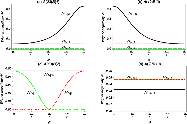
Figure 10: WNs versus $\phi$ with fixed $\bar{n}_{T}=3$, for some $\rho_{B_{a}|A}$s in cases (a) $A(23)B(1)$, (b) $A(12)B(3)$, (c) $A(13)B(2)$, and (d) $A(2)B(13)$.

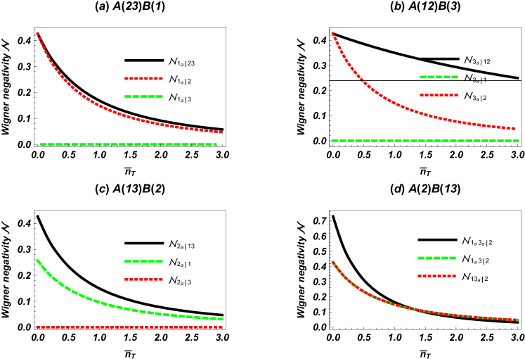
Figure 11: WNs versus $\bar{n}_{T}$ with fixed $\phi=\pi/8$, for some $\rho_{B_{a}|A}$s in cases (a) $A(23)B(1)$, (b) $A(12)B(3)$, (c) $A(13)B(2)$, and (d) $A(2)B(13)$.

Case $A(23)B(1)$: In this case, the steering party $A$ includes mode 2 and mode 3 and the steered party $B$ includes mode 1. Performing appropriate photon subtraction(s) in the local position, we can remotely generate the following states with their respective WNs:

$$\rho_{1_{a}|23} = \mathrm{Tr}_{1}\left(\rho_{1_{a}23}\right)\rightarrow\mathcal{N}_{1_{a}|23},$$

$$\rho_{1_{a}|2} = \mathrm{Tr}_{1,3}\left(\rho_{1_{a}23}\right)\rightarrow\mathcal{N}_{1_{a}|2},$$

$$\rho_{1_{a}|3} = \mathrm{Tr}_{1,2}\left(\rho_{1_{a}23}\right)\rightarrow\mathcal{N}_{1_{a}|3},$$ (27)

where $\rho_{1_{a}23}=\left|\epsilon_{1}\right|_{1}^{-2}\hat{a}_{1}\rho_{123}\hat{a}_{1}^{{\dagger}}$.

We plot $\mathcal{N}_{1_{a}|23}$, $\mathcal{N}_{1_{a}|2}$, and $\mathcal{N}_{1_{a}|3}$ as functions of $\phi$ in Fig.10(a) and as functions of $\bar{n}_{T}$ in Fig.11(a). From these figures, we find that WNs are generated remotely in the group (23), mode 2 and mode 3, respectively, after a single-photon subtraction on mode 1. Moreover, we see that (i) $\mathcal{N}_{1_{a}|23}$ is a monotonically increasing function of $\phi$ from $0.04682$ at $\phi=0$ to $0.42614$ at $\phi=\pi/2$; (ii) $\mathcal{N}_{1_{a}|2}\$ remains as $0.04682$ for any $\phi$; (iii) $\mathcal{N}_{1_{a}|3}\$ remains as $0$ for any $\phi$; (iv) $\mathcal{N}_{1_{a}|23}\geq\mathcal{N}_{1_{a}|2}+\mathcal{N}_{1_{a}|3}$; and (v) as $\bar{n}_{T}$ is increasing, all these WNs will be limited to $0$.

Case $A(12)B(3)$: In this case, the steering party $A$ include mode 1 and mode 2 and the steered party $B$ include mode 3. Performing appropriate photon subtraction(s) in the local position, we can remotely generate the following states with their respective WNs:

$$\rho_{3_{a}|12} = \mathrm{Tr}_{3}\left(\rho_{123_{a}}\right)\rightarrow\mathcal{N}_{3_{a}|12},$$

$$\rho_{3_{a}|1} = \mathrm{Tr}_{2,3}\left(\rho_{123_{a}}\right)\rightarrow\mathcal{N}_{3_{a}|1},$$

$$\rho_{3_{a}|2} = \mathrm{Tr}_{1,3}\left(\rho_{123_{a}}\right)\rightarrow\mathcal{N}_{3_{a}|2},$$ (28)

where $\rho_{123_{a}}=\left|\epsilon_{2}\right|^{-2}\hat{a}_{3}\rho_{123}\hat{a}_{3}^{{\dagger}}$.

We plot $\mathcal{N}_{3_{a}|12}$, $\mathcal{N}_{3_{a}|1}$, and $\mathcal{N}_{3_{a}|2}$ as functions of $\phi$ in Fig.10(b) and as functions of $\bar{n}_{T}$ in Fig.11(b). From these figures, we find that WNs are generated remotely in the group (12), mode 1 and mode 2, respectively, after a single-photon subtraction on mode 3. Moreover, we see that (i) $\mathcal{N}_{3_{a}|12}$ is a monotonically decreasing function of $\phi$ from $0.42614$ at $\phi=0$ to $0.04682$ at $\phi=\pi/2$; (ii) $\mathcal{N}_{3_{a}|2}\$ remains as $0.04682$ for any $\phi$; (iii) $\mathcal{N}_{3_{a}|1}\$ remains as $0$ for any $\phi$; (iv) $\mathcal{N}_{3_{a}|12}\geq\mathcal{N}_{3_{a}|1}+\mathcal{N}_{3_{a}|2}$; and (v) as $\bar{n}_{T}$ is increasing, all these WNs will be limited to $0$.

Case $A(13)B(2)$: In this case, the steering party $A$ includes mode 1 and mode 3 and the steered party $B$ includes mode 2. Performing appropriate photon subtraction(s) in the local position, we can remotely generate the following states with their respective WNs:

$$\rho_{2_{a}|13} = \mathrm{Tr}_{2}\left(\rho_{12_{a}3}\right)\rightarrow\mathcal{N}_{2_{a}|13},$$

$$\rho_{2_{a}|1} = \mathrm{Tr}_{2,3}\left(\rho_{12_{a}3}\right)\rightarrow\mathcal{N}_{2_{a}|1},$$

$$\rho_{2_{a}|3} = \mathrm{Tr}_{1,2}\left(\rho_{12_{a}3}\right)\rightarrow\mathcal{N}_{2_{a}|3},$$ (29)

where $\rho_{12_{a}3}=s^{-2}\hat{a}_{2}\rho_{123}\hat{a}_{2}^{{\dagger}}$.

We plot $\mathcal{N}_{2_{a}|13}$, $\mathcal{N}_{2_{a}|1}$, and $\mathcal{N}_{2_{a}|3}$ as functions of $\phi$ in Fig.10(c) and as functions of $\bar{n}_{T}$ in Fig.11(c). From these figures, we find that WNs are generated remotely in the group (13), mode 1 and mode 3, respectively, after a single-photon subtraction on mode 2. Moreover, we see that (i) $\mathcal{N}_{2_{a}|13}$ remains as $0.4683$ for any $\phi$; (ii) $\mathcal{N}_{2_{a}|1}$ decreases from $0.4683$ to $0$ in $\left[0,\pi/4\right]$ and remains as $0$ in $\left[\pi/4,\pi/2\right]$; (iii) $\mathcal{N}_{2_{a}|3}$ remains as $0$ in $\left[0,\pi/4\right]$ and increases from $0$ to $0.4683$ in $\left[\pi/4,\pi/2\right]$; (iv) $\mathcal{N}_{2_{a}|13}\geq\mathcal{N}_{2_{a}|1}+\mathcal{N}_{2_{a}|3}$; and (v) as $\bar{n}_{T}$ is increasing, all these WNs will be limited to $0$.

Case $A(2)B(13)$: In this case, the steering party $A$ include mode 2 and the steered party $B$ include mode 1 and mode 3. Performing appropriate photon subtraction(s) in the local position, we can remotely generate the following states with their respective WNs:

$$\rho_{1_{a}3_{a}|2} = \mathrm{Tr}_{1,3}\left(\rho_{1_{a}23_{a}}\right)\rightarrow\mathcal{N}_{1_{a}3_{a}|2},$$

$$\rho_{1_{a}3|2} = \mathrm{Tr}_{1,3}\left(\rho_{1_{a}23}\right)\rightarrow\mathcal{N}_{1_{a}3|2},$$

$$\rho_{13_{a}|2} = \mathrm{Tr}_{1,3}\left(\rho_{123_{a}}\right)\rightarrow\mathcal{N}_{13_{a}|2},$$ (30)

where $\rho_{1_{a}23_{a}}=\frac{1}{2}\left|\epsilon_{1}\epsilon_{2}\right|^{-2}\hat{a}_{1}\hat{a}_{3}\rho_{123}\hat{a}_{1}^{{\dagger}}\hat{a}_{3}^{{\dagger}}$.

We plot $\mathcal{N}_{1_{a}3_{a}|2}$, $\mathcal{N}_{1_{a}3|2}$, and $\mathcal{N}_{13_{a}|2}$ as functions of $\phi$ in Fig.10(d) and as functions of $\bar{n}_{T}$ in Fig.11(d). From these figures, we find that WNs are generated remotely in mode 2, after single-photon subtractions on each mode of the group (13) simultaneously, or after a single-photon subtraction on mode 1 or mode 3, respectively. Here, we see that (1) $\mathcal{N}_{1_{a}3_{a}|2}$ remains as $0.0318528$, (2) $\mathcal{N}_{1_{a}3|2}$ and $\mathcal{N}_{13_{a}|2}\$remain as $0.04683$; (3) $\mathcal{N}_{1_{a}3_{a}|2}<\mathcal{N}_{1_{a}3|2}+\mathcal{N}_{13_{a}|2}$; (4) As $\bar{n}_{T}$ increasing, all these WNs will limit to $0$. However, although $\mathcal{G}^{2\rightarrow 1}>0$, $\mathcal{G}^{2\rightarrow 3}>0$, and $\mathcal{G}^{2\rightarrow\left(31\right)}>0$, we cannot achieve more significant increase of the WNs in mode 2, after performing a single-photon subtraction on each of mode 1 and mode 3.

Case $A(1)B(23)$: In this case, the steering party $A$ include mode 1 and the steered party $B$ include mode 2 and mode 3. Performing appropriate photon subtraction(s) in the local position, we can remotely generate the following states with their respective WNs:

$$\rho_{2_{a}3_{a}|1} = \mathrm{Tr}_{2,3}\left(\rho_{12_{a}3_{a}}\right)\rightarrow\mathcal{N}_{2_{a}3_{a}|1}\equiv 0,$$

$$\rho_{2_{a}3|1} = \mathrm{Tr}_{2,3}\left(\rho_{12_{a}3}\right)\rightarrow\mathcal{N}_{2_{a}3|1}\equiv 0,$$

$$\rho_{23_{a}|1} = \mathrm{Tr}_{2,3}\left(\rho_{123_{a}}\right)\rightarrow\mathcal{N}_{23_{a}|1}\equiv 0,$$ (31)

where $\rho_{12_{a}3_{a}}=\left(c^{2}+s^{2}\right)^{-1}\left|\epsilon_{2}\right|^{-2}\hat{a}_{2}\hat{a}_{3}\rho_{123}\hat{a}_{2}^{{\dagger}}\hat{a}_{3}^{{\dagger}}$. For any $\bar{n}_{T}$ and $\phi$, we see $\mathcal{N}_{2_{a}3_{a}|1}=\mathcal{N}_{2_{a}3|1}=\mathcal{N}_{23_{a}|1}\equiv 0$. That is to say, no WNs are generated remotely in mode 1, after single-photon subtractions on each mode of the group (23) simultaneously, or after a single-photon subtraction on mode 2 or mode 3. Surprisingly, $\mathcal{N}_{2_{a}3_{a}|1}=0$ although $\mathcal{G}^{1\rightarrow 23}>0$.

Case $A(3)B(12)$: In this case, the steering party $A$ include mode-3 and the steered party $B$ include mode 1 and mode 2. Performing appropriate photon subtraction(s) in the local position, we can remotely generate the following states with their respective WNs:

$$\rho_{1_{a}2_{a}|3} = \mathrm{Tr}_{1,2}\left(\rho_{1_{a}2_{a}3}\right)\rightarrow\mathcal{N}_{1_{a}2_{a}|3}\equiv 0,$$

$$\rho_{1_{a}2|3} = \mathrm{Tr}_{1,2}\left(\rho_{1_{a}23}\right)\rightarrow\mathcal{N}_{1_{a}2|3}\equiv 0,$$

$$\rho_{12_{a}|3} = \mathrm{Tr}_{1,2}\left(\rho_{12_{a}3}\right)\rightarrow\mathcal{N}_{12_{a}|3}\equiv 0,$$ (32)

where $\rho_{1_{a}2_{a}3}=\left(c^{2}+s^{2}\right)^{-1}\left|\epsilon_{1}\right|^{-2}\hat{a}_{1}\hat{a}_{2}\rho_{123}\hat{a}_{1}^{{\dagger}}\hat{a}_{2}^{{\dagger}}$. For any $\bar{n}_{T}$ and $\phi$, we see $\mathcal{N}_{1_{a}2_{a}|3}=\mathcal{N}_{1_{a}2|3}=\mathcal{N}_{12_{a}|3}\equiv 0$. That is to say, no WNs are generated remotely in mode 3, after single-photon subtractions on each mode of the group (12) simultaneously, or after a single-photon subtraction on mode 1 or mode 2. Surprisingly, $\mathcal{N}_{1_{a}2_{a}|3}=0$ although $\mathcal{G}^{3\rightarrow 12}>0$.

So far, we have quantified all remotely generated WNs in terms of Eq.(26). It is obvious to see that the amount of WN cannot be freely distributed among different modes.

VI Conclusion and discussion

To summarize, we studied the C3MSV and showed how it can be used for steering. By taking different bipartite assignment in the C3MSV, we investigated all bipartite Gaussian steerings present in the C3MSV. These steerings include no steering, one-way steering and two-way steering. Moreover, the steerability can be adjusted by the interaction parameters. In addition, we also studied the decoherence of the steering for the C3MSV and found that the steering will die suddenly at a threshold time. Using the C3MSV as the resource, we proposed conceptual schemes to remotely generate Wigner negative states. We analyzed and compared the distributions of the Gaussian steering and the WNs over different modes. Normally, one expect that stronger steerability induces more WN. That is, if $\mathcal{G}^{A\rightarrow B}>0$, then $\mathcal{N}>0$; and if $\mathcal{G}^{A\rightarrow B}=0$, then $\mathcal{N}=0$. But this is not the case for the C3MSV. For example, although $\mathcal{G}^{1\rightarrow 23}>0$ and $\mathcal{G}^{3\rightarrow 12}>0$, $\rho_{2_{a}3_{a}|1}$ and $\rho_{1_{a}2_{a}|3}$ cannot exhibit WN. These results further verify that quantum correlations are not always a necessary requirement for the conditional generation of WN57 .

People expect that the correlations can be more robust to environmental influences (including loss and noise) 89 ; 90 . Meanwhile, measurement will have nonunity detection efficiency 91 ; 92 accompanied with information leakage 93 . With the help of squeezed states 94 and erasure corrections 95 , one can establish quantum optical coherence over longer distances to diminish the effect from losses and noises. In the aspects of experiment and measurement, our paper is a reservoir of more discussions. Although our work is theoretical and ideal, we still believe that our results may also lay a solid theoretical foundation for a future practical study.

Practical quantum communications (including quantum internet 96 ; 97 , satellite communication 98 , and online banking 99 ) require multipartite correlation and high security 100 ; 101 . Fortunately, all these problems will solved by using protocols involved in quantum steering 102 . Specific properties of the C3MSV (including squeezing, entanglement and steering) have laid a good foundation for applications in quantum technologies. So, we believe the C3MSV will become a useful entangled resource in future quantum communication. For example, following previous works65 ; 66 ; 103 and using the C3MSV, one can construct a new scheme to teleclone pure Gaussian states.

Appendix A: The C3MSO and the C3MSV

In this appendix, we give the transformation relation and the normal ordering form for the C3MSO. In addition, we give the general expression to calculate the expectation values we want for the C3MSV.

About the C3MSO. Using the formula of Bogoliubov transformation, we obtain the following transformation relations

$$S_{3}A^{{\dagger}}S_{3}^{{\dagger}}=A^{{\dagger}}P^{\ast}+AL^{\ast},S_{3}AS_{3}^{{\dagger}}=AP+A^{{\dagger}}L,$$ (A.1)

where $A^{{\dagger}}=\left(\hat{a}_{1}^{{\dagger}},\hat{a}_{2}^{{\dagger}},\hat{a}_{3}^{{\dagger}}\right)$, $A=\left(\hat{a}_{1},\hat{a}_{2},\hat{a}_{3}\right)$, and

$$P=\left(\begin{array}[]{ccc}\kappa_{1}&0&\tau\\ 0&c&0\\ \tau^{\ast}&0&\kappa_{2}\end{array}\right),L=\left(\begin{array}[]{ccc}0&\epsilon_{1}&0\\ \epsilon_{1}&0&\epsilon_{2}\\ 0&\epsilon_{2}&0\end{array}\right).$$ (A.2)

Here we set $\kappa_{1}=\sin^{2}\phi+c\cos^{2}\phi$, $\kappa_{2}=\cos^{2}\phi+c\sin^{2}\phi$, and $\tau=\frac{1}{2}(c-1)e^{i(\theta_{2}-\theta_{1})}\sin 2\phi$.

According to the rule provided by Fan and co-workers104 ; 105 ; 106 , we immediately obtain the normal ordering form of $S_{3}$ as follows

$$S_{3} =\frac{1}{\sqrt{\det P}}e^{-\frac{1}{2}A^{{\dagger}}(LP^{-1})\tilde{A}^{{\dagger}}}$$

$$:e^{A^{{\dagger}}(\tilde{P}^{-1}-I)\tilde{A}}:e^{\frac{1}{2}A(P^{-1}L^{\ast})\tilde{A}}.$$ (A.3)

Of course, we can further use $:e^{A^{{\dagger}}(\tilde{P}^{-1}-I)\tilde{A}}:=e^{A^{{\dagger}}(\ln\tilde{P}^{-1})\tilde{A}}$ in above expression, where $\tilde{P}$ denotes the transpose of $P$.

About the C3MSV. Here, we give the following general expression of expectation value:

$$\left\langle\hat{a}_{1}^{{\dagger}k_{1}}\hat{a}_{2}^{{\dagger}k_{2}}\hat{a}_{3}^{{\dagger}k_{3}}\hat{a}_{1}^{l_{1}}\hat{a}_{2}^{l_{2}}\hat{a}_{3}^{l_{3}}\right\rangle$$

$$=\partial_{\mu_{1}}^{k_{1}}\partial_{\mu_{2}}^{k_{2}}\partial_{\mu_{3}}^{k_{3}}\partial_{\nu_{1}}^{l_{1}}\partial_{\nu_{2}}^{l_{2}}\partial_{\nu_{3}}^{l_{3}}$$

$$e^{\left|\epsilon_{1}\right|^{2}\mu_{1}\nu_{1}+s^{2}\mu_{2}\nu_{2}+\left|\epsilon_{2}\right|^{2}\mu_{3}\nu_{3}+\epsilon_{1}^{\ast}\epsilon_{2}\mu_{1}\nu_{3}+\epsilon_{1}\epsilon_{2}^{\ast}\mu_{3}\nu_{1}}$$

$$e^{-c\epsilon_{1}^{\ast}\mu_{1}\mu_{2}-c\epsilon_{1}\nu_{1}\nu_{2}-c\epsilon_{2}^{\ast}\mu_{2}\mu_{3}-c\epsilon_{2}\nu_{2}\nu_{3}}$$

$$|_{\mu_{1}=\mu_{2}=\mu_{3}=\nu_{1}=\nu_{2}=\nu_{3}=0},$$ (A.4)

from which one can study the statistical properties for the C3MSV. Notice that $k_{1}$, $k_{2}$, $k_{3}$, $l_{1}$, $l_{2}$, and $l_{3}$ are non-negative integers.

Appendix B: Derivation of evolution relation in the reservoir

Using the Laplace transformation

$$\tilde{a}_{j}\left(p\right)=\mathrm{LT}\left[a_{j}\left(t\right)\right]=\int_{0}^{\infty}dt\exp\left(-pt\right)a_{j}\left(t\right),$$ (B1)

and $\mathrm{LT}\left[\dot{a}_{j}\left(t\right)\right]=p\tilde{a}_{j}\left(p\right)-a_{j}\left(0\right)$, Eq.(24) yields

$$\tilde{a}_{j}\left(p\right)=\frac{1}{p+\gamma_{j}}a_{j}\left(0\right)+\sqrt{2\gamma_{j}}\frac{\tilde{\Gamma}_{j}\left(p\right)}{p+\gamma_{j}}$$ (B2)

which leads to 80

$$a_{j}\left(t\right)=e^{-\gamma_{j}t}a_{j}\left(0\right)+\sqrt{2\gamma_{j}}\int_{0}^{t}e^{-\gamma_{j}(t-\tau)}\Gamma_{j}\left(\tau\right)d\tau.$$ (B3)

Notice that the quantum reservoir operators have correlations given by $\left\langle\Gamma_{j}\right\rangle=\left\langle\Gamma_{j}^{{\dagger}}\right\rangle=\left\langle\Gamma_{j}^{2}\right\rangle=\left\langle\Gamma_{j}^{{\dagger}2}\right\rangle=0$ and

$$\left\langle\Gamma_{j}^{{\dagger}}\left(\tau^{\prime}\right)\Gamma_{j}\left(\tau\right)\right\rangle =\bar{n}_{R_{j}}\delta\left(\tau^{\prime}-\tau\right)$$

$$\left\langle\Gamma_{j}\left(\tau\right)\Gamma_{j}^{{\dagger}}\left(\tau^{\prime}\right)\right\rangle =(\bar{n}_{R_{j}}+1)\delta\left(\tau^{\prime}-\tau\right).$$ (B4)

as well as $\left\langle\Gamma_{j}\Gamma_{k}\right\rangle=\left\langle\Gamma_{j}^{{\dagger}}\Gamma_{k}^{{\dagger}}\right\rangle=\left\langle\Gamma_{j}\Gamma_{k}^{{\dagger}}\right\rangle=\left\langle\Gamma_{j}^{{\dagger}}\Gamma_{k}\right\rangle=0$ for $j\neq k$. Thus we can calculate the moments at a later time in terms of the initial moments, in terms of the relations such as $\left\langle a_{j}\left(t\right)\right\rangle=e^{-\gamma_{j}t}\left\langle a_{j}\left(0\right)\right\rangle$, $\left\langle a_{j}^{2}\left(t\right)\right\rangle=e^{-2\gamma_{j}t}\left\langle a_{j}^{2}\left(0\right)\right\rangle$, and

$$\left\langle a_{j}^{{\dagger}}\left(t\right)a_{j}\left(t\right)\right\rangle =e^{-2\gamma_{j}t}\left\langle a_{j}^{{\dagger}}\left(0\right)a_{j}\left(0\right)\right\rangle$$

$$+\bar{n}_{R_{j}}\left(1-e^{-2\gamma_{j}t}\right)$$ (B5)

for the same mode, as well as

$$\left\langle a_{j}\left(t\right)a_{k}\left(t\right)\right\rangle =e^{-(\gamma_{j}+\gamma_{k})t}\left\langle a_{j}\left(0\right)a_{k}\left(0\right)\right\rangle$$

$$\left\langle a_{j}^{{\dagger}}\left(t\right)a_{k}\left(t\right)\right\rangle =e^{-(\gamma_{j}+\gamma_{k})t}\left\langle a_{j}^{{\dagger}}\left(0\right)a_{k}\left(0\right)\right\rangle$$ (B6)

for different modes.

Appendix C: Wigner functions of remotely generated states

The WF for the C3MSV is

$$W_{\rho_{123}} =\frac{8}{\pi^{3}}e^{-2[\left(2\bar{n}_{1}+1\right)\left|\beta_{1}\right|^{2}+\left(2\bar{n}_{2}+\allowbreak 1\right)\left|\beta_{2}\right|^{2}+\left(2\bar{n}_{3}+1\right)\left|\beta_{3}\right|^{2}]}$$

$$\times e^{-8[\text{Re}(c\epsilon_{1}^{\ast}\beta_{1}\beta_{2}\allowbreak)+\text{Re}(\epsilon_{1}^{\ast}\epsilon_{2}\beta_{1}\beta_{3}^{\ast})+\text{Re}(c\epsilon_{2}^{\ast}\allowbreak\beta_{2}\beta_{3})]},$$ (C1)

which has the Gaussian form.

The analytical WFs of $\rho_{B_{a}|A}$s are given as follows. For convenience of writing, we set $\omega_{0}=c^{2}+s^{2}=\cosh 2r$, $\omega_{1}=c^{2}-s^{2}\cos 2\phi$, and $\omega_{2}=c^{2}+s^{2}\cos 2\phi$. If $\phi=0$, then $\epsilon_{2}=0$, $r=r_{1}$, $\omega_{1}=1$ and $\omega_{2}=\omega_{0}$. If $\phi=\pi/2$, then $\epsilon_{1}=0$, $r=r_{2}$, $\omega_{1}=\omega_{0}$, and $\omega_{2}=1$.

(a) The WF for $\rho_{1_{a}|23}$ is obtained by

$$W_{\rho_{1_{a}|23}} =\frac{4e^{-2[\omega_{1}\left|\beta_{2}\right|^{2}+\omega_{0}\left|\beta_{3}\right|^{2}+4\text{Re}(c\epsilon_{2}^{\ast}\beta_{2}\beta_{3})]/\omega_{2}}}{\pi^{2}\omega_{2}^{3}}$$

$$\times(4\left|c\beta_{2}+\epsilon_{2}\beta_{3}^{\ast}\right|^{2}-\omega_{2}).$$ (C2)

When $\phi=0$, Eq.(C2) will be reduced to $W_{\rho_{1_{a}|23}}=(2/\pi)e^{-2\left|\beta_{2}\right|^{2}/\omega_{0}}(4c^{2}\omega_{0}^{-3}\left|\beta_{2}\right|^{2}-\omega_{0}^{-2})\times(2/\pi)e^{-2\left|\beta_{3}\right|^{2}}$.

(b) The WF for $\rho_{2_{a}|13}$ is obtained by

$$W_{\rho_{2_{a}|13}} =\frac{4e^{-2[\omega_{1}\left|\beta_{1}\right|^{2}+\omega_{2}\allowbreak\left|\beta_{3}\right|^{2}-4\text{Re}(\epsilon_{1}^{\ast}\epsilon_{2}\beta_{1}\allowbreak\beta_{3}^{\ast})]/\omega_{0}}}{\pi^{2}s^{2}\omega_{0}^{3}}$$

$$\times(4c^{2}\left|\epsilon_{1}^{\ast}\beta_{1}+\epsilon_{2}^{\ast}\beta_{3}\right|^{2}-\omega_{0}s^{2}\allowbreak).$$ (C3)

When $\phi=0$, Eq.(C3) will be reduced to $W_{\rho_{2_{a}|13}}=(2/\pi)e^{-2\left|\beta_{1}\right|^{2}/\omega_{0}}(4c^{2}\omega_{0}^{-3}\cos^{2}\phi\left|\beta_{1}\right|^{2}-\omega_{0}^{-2})\times(2/\pi)e^{-2\left|\beta_{3}\right|^{2}}$; When $\phi=\pi/2$, Eq.(C3) will be reduced to $W_{\rho_{2_{a}|13}}=(2/\pi)e^{-2\left|\beta_{3}\right|^{2}/\omega_{0}}(4c^{2}\omega_{0}^{-3}\sin^{2}\phi\left|\beta_{3}\right|^{2}-\omega_{0}^{-2})\times(2/\pi)e^{-2\left|\beta_{1}\right|^{2}}$.

(c) The WF for $\rho_{3_{a}|12}$ is obtained by

$$W_{\rho_{3_{a}|12}} =\frac{4e^{-2[\omega_{2}\left|\beta_{2}\right|^{2}+\omega_{0}\left|\beta_{1}\right|^{2}+4\text{Re}(c\epsilon_{1}^{\ast}\beta_{1}\beta_{2})]/\omega_{1}}}{\pi^{2}\omega_{1}^{3}}$$

$$\times(4\left|c\beta_{2}+\epsilon_{1}\beta_{1}^{\ast}\right|^{2}-\omega_{1}).$$ (C4)

When $\phi=\pi/2$, Eq.(C4) will be reduced to $W_{\rho_{3_{a}|12}}=(2/\pi)e^{-2\left|\beta_{2}\right|^{2}/\omega_{0}}(4c^{2}\omega_{0}^{-3}\left|\beta_{2}\right|^{2}-\omega_{0}^{-2})\times(2/\pi)e^{-2\left|\beta_{1}\right|^{2}}$.

(d) The WF for $\rho_{2_{a}3_{a}|1}$ is obtained by

$$W_{\rho_{2_{a}3_{a}|1}} =\frac{2e^{-2\left|\beta_{1}\right|^{2}/\omega_{2}}}{\pi\omega_{0}\omega_{2}^{5}}$$

$$\times[\omega_{2}^{2}\allowbreak\omega_{1}+4\left|\epsilon_{1}\beta_{1}\right|^{2}(4c^{4}+4c^{2}\left|\epsilon_{1}\beta_{1}\right|^{2}-\omega_{1}^{2})]$$ (C5)

When $\phi=\pi/2$, Eq.(C5) will be reduced to $W_{\rho_{2_{a}3_{a}|1}}=(2/\pi)e^{-2\left|\beta_{1}\right|^{2}}$.

(e) The WF for $\rho_{1_{a}3_{a}|2}$ is obtained by

$$W_{\rho_{1_{a}3_{a}|2}}=\frac{2e^{-2\left|\beta_{2}\right|^{2}/\omega_{0}}}{\pi\omega_{0}^{5}}(\omega_{0}^{2}\allowbreak+8c^{4}\left|\beta_{2}\right|^{4}-8\omega_{0}c^{2}\left|\beta_{2}\right|^{2}),$$ (C6)

which is independent of $\phi$.

(f) The WF for $\rho_{1_{a}2_{a}|3}$ is obtained by

$$W_{\rho_{1_{a}2_{a}|3}} =\frac{2e^{-2\left|\beta_{3}\right|^{2}/\omega_{1}}}{\pi\omega_{0}\omega_{1}^{5}}\allowbreak$$

$$\times[\omega_{1}^{2}\allowbreak\omega_{2}+4\left|\epsilon_{2}\beta_{3}\right|^{2}(4c^{4}\allowbreak+4c^{2}\left|\epsilon_{2}\beta_{3}\right|^{2}-\omega_{2}^{2})].$$ (C7)

When $\phi=0$, Eq.(C7) will be reduced to $W_{\rho_{1_{a}2_{a}|3}}=(2/\pi)e^{-2\left|\beta_{3}\right|^{2}}$.

(g) The WFs for $\rho_{1_{a}|2}$ and $\rho_{1_{a}3|2}$ are obtained by

$$W_{\rho_{1_{a}|2}}=W_{\rho_{1_{a}3|2}}=\frac{2e^{-2\left|\beta_{2}\right|^{2}/\omega_{0}}}{\pi\omega_{0}^{3}}(4c^{2}\left|\beta_{2}\right|^{2}-\omega_{0}),$$ (C8)

which is independent of $\phi$.

(h) The WFs for $\rho_{3_{a}|1}$ and $\rho_{23_{a}|1}$ are obtained by

$$W_{\rho_{3_{a}|1}}=W_{\rho_{23_{a}|1}}=\frac{\allowbreak 2e^{-\allowbreak 2\left|\beta_{1}\right|^{2}/\omega_{2}}}{\pi\omega_{2}^{3}}(4\left|\epsilon_{1}\beta_{1}\right|^{2}+\omega_{2}).$$ (C9)

When $\phi=\pi/2$, Eq.(C9) will be reduced to $W_{\rho_{3_{a}|1}}=W_{\rho_{23_{a}|1}}=(2/\pi)e^{-2\left|\beta_{1}\right|^{2}}$.

(i) The WFs for $\rho_{3_{a}|2}$ and $\rho_{13_{a}|2}$ are obtained by

$$W_{\rho_{3_{a}|2}}=W_{\rho_{13_{a}|2}}=\frac{2e^{-2\left|\beta_{2}\right|^{2}/\omega_{0}}}{\pi\omega_{0}^{3}}(4c^{2}\left|\beta_{2}\right|^{2}-\omega_{0}),$$ (C10)

which is independent of $\phi$.

(j) The WFs for $\rho_{2_{a}|1}$ and $\rho_{2_{a}3|1}$ are obtained by

$$W_{\rho_{2_{a}|1}} =W_{\rho_{2_{a}3|1}}$$

$$=\frac{2e^{-2\left|\beta_{1}\right|^{2}/\omega_{2}}}{\pi\omega_{2}^{3}}(4c^{2}\left|\beta_{1}\right|^{2}\allowbreak\cos^{2}\phi-\omega_{2}\cos 2\phi).$$ (C11)

When $\phi=\pi/2$, Eq.(C11) will be reduced to $W_{\rho_{2_{a}|1}}=W_{\rho_{2_{a}3|1}}=(2/\pi)e^{-2\left|\beta_{1}\right|^{2}}$.

(k) The WFs for $\rho_{1_{a}|3}$ and $\rho_{1_{a}2|3}$ are obtained by

$$W_{\rho_{1_{a}|3}}=W_{\rho_{1_{a}2|3}}=\frac{2e^{-\allowbreak 2\left|\beta_{3}\right|^{2}/\omega_{1}}}{\pi\omega_{1}^{3}}\allowbreak(4\left|\epsilon_{2}\beta_{3}\right|^{2}+\omega_{1}).$$ (C12)

When $\phi=0$, Eq.(C12) will be reduced to $W_{\rho_{1_{a}|3}}=W_{\rho_{1_{a}2|3}}=(2/\pi)e^{-2\left|\beta_{3}\right|^{2}}$.

(l) The WFs for $\rho_{2_{a}|3}$ and $\rho_{12_{a}|3}$ are obtained by

$$W_{\rho_{2_{a}|3}} =W_{\rho_{12_{a}|3}}$$

$$=\frac{2e^{-2\left|\beta_{3}\right|^{2}/\omega_{1}}}{\pi\omega_{1}^{3}}(4c^{2}\left|\beta_{3}\right|^{2}\allowbreak\sin^{2}\phi+\omega_{1}\cos 2\phi).$$ (C13)

When $\phi=0$, Eq.(C13) will be reduced to $W_{\rho_{2_{a}|3}}=W_{\rho_{12_{a}|3}}=(2/\pi)e^{-2\left|\beta_{3}\right|^{2}}$.

References

- (1) K. Modi, A. Brodutch, H. Cable, T. Paterek, and V. Vedral, The classical-quantum boundary for correlations: Discord and related measures, Rev. Mod. Phys. 84, 1655 (2012).
- (2) C. H. Bennett, G. Brassard, C. Crepeau, R. Jozsa, A. Peres, and W. K. Wootters, Teleporting an unknown quantum state via dual classical and Einstein-Podolsky-Rosen channels, Phys. Rev. Lett. 70, 1895 (1993).
- (3) R. Horodecki, P. Horodecki, M. Horodecki, and K. Horodecki, Quantum entanglement, Rev. Mod. Phys. 81, 865 (2009).
- (4) M. D. Reid, P. D. Drummond, W. P. Bowen, E. G. Cavalcanti, P. K. Lam, H. A. Bachor, U. L. Andersen, and G. Leuchs, The Einstein-Podolsky-Rosen paradox: From concepts to applications, Rev. Mod. Phys. 81, 1727 (2009).
- (5) R. Uola, A. C. S. Costa, H. Chau Nguyen, and O. Guhne, Quantum steering, Rev. Mod. Phys. 92, 015001 (2020).
- (6) L. M. Duan, G. Giedke, J. I. Cirac, and P. Zoller, Inseparability Criterion for Continuous Variable Systems, Phys. Rev. Lett. 84, 2722 (2000).
- (7) J. S. Bell, On the Einstein podolsky rosen paradox, Physics 1, 195 (1964).
- (8) N. Brunner, D. Cavalcanti, S. Pironio, V. Scarani, and S. Wehner, Bell nonlocality, Phys. Mod. Phys. 86, 419 (2014).
- (9) V. Scarani, Bell Nonlocality (Oxford University, Oxford, 2019).
- (10) I. Kogias, A. R. Lee, S. Ragy, and G. Adesso, Quantification of Gaussian Quantum Steering, Phys. Rev. Lett. 114, 060403 (2015).
- (11) P. Skrzypczyk, M. Navascues, and D. Cavalcanti, Quantifying Einstein-Podolsky-Rosen Steering, Phys. Rev. Lett. 112, 180404 (2014).
- (12) Q. Y. He, Q. H. Gong, and M. D. Reid, Classifying Directional Gaussian Entanglement, Einstein-Podolsky-Rosen Steering, and Discord, Phys. Rev. Lett. 114, 060402 (2015).
- (13) S. Armstrong, M. Wang, R. Y. Teh, Q. H. Gong, Q. Y. He, J. Janousek, H. A. Bachor, M. D. Reid, and P. K. Lam, Multipartite Einstein-Podolsky-Rosen steering and genuine tripartite entanglement with optical networks, Nat. Phys. 11, 167 (2015).
- (14) Q. Y. He and M. D. Reid, Genuine Multipartite Einstein-Podolsky-Rosen Steering, Phys. Rev. Lett. 111, 250403 (2013).
- (15) E. Schrodinger, Discussion of probability relations between separated systems, Math. Proc. Cambridge Philos. Soc. 31, 555 (1935).
- (16) H. M. Wiseman, S. J. Jones, and A. C. Doherty, Steering, Entanglement, Nonlocality, and the Einstein-Podolsky-Rosen Paradox, Phys. Rev. Lett. 98, 140402 (2007).
- (17) S. J. Jones, H. M. Wiseman, and A. C. Doherty, Entanglement, Einstein-Podolsky-Rosen correlations, Bell nonlocality, and steering, Phys. Rev. A 76, 052116 (2007).
- (18) C. Wilkinson, M. Thornton, and N. Korolkova, Quantum steering as a resource for secure tripartite quantum state sharing, Phys. Rev. A 107, 062401 (2023).
- (19) Y. Cai, Y. Xiang, Y. Liu, Q. He, and N. Treps, Versatile multipartite Einstein-Podolsky-Rosen steering via a quantum frequency comb, Phys. Rev. Research 2, 032046(R) (2020).
- (20) H. P. Yuen and J. H. Shapiro, Generation and detection of two-photon coherent states in degenerate four-wave mixing, Opt. Lett. 4, 334 (1979).
- (21) U. L Andersen, T. Gehring, C. Marquardt and G. Leuchs, 30 years of squeezed light generation, Phys. Scr. 91, 053001 (2016).
- (22) N. J. Cerf and G. Leuchs, Quantum Information with Continuous Variables of Atoms and Light (Imperial College, London 2007).
- (23) R. W. Boyd, Nonlinear Optics, 3rd ed. (Academic, San Diego, 2008).
- (24) D. F. Walls and D. J. Milburn, Quantum Optics (Springer-Verlag, Berlin, 1994).
- (25) M. D. Reid and D. F. Walls, Generation of squeezed states via degenerate four-wave mixing, Phys. Rev. A 31, 1622 (1985).
- (26) M. O. Scully and M. S. Zubairy, Quantum Optics (Cambridge University, Cambridge, England, 1997).
- (27) Y. Xiang, F. Sun, Q. He, Q. Gong, Advances in multipartite and high-dimensional Einstein-Podolsky-Rosen steering, Fundamental Research 1, 99 (2021).
- (28) S. S. Liu, H. L. Wang, and J. T. Jing, Two-beam pumped cascaded four-wave-mixing process for producing multiple-beam quantum correlation, Phys. Rev. A 97, 043846 (2018).
- (29) K. Zhang, W. Wang, S. Liu, X. Pan, J. Du, Y. Lou, S. Yu, S. Lv, N. Treps, C. Fabre, and J. T. Jing, Reconfigurable Hexapartite Entanglement by Spatially Multiplexed Four-Wave Mixing Processes, Phys. Rev. Lett. 124, 090501 (2020).
- (30) H. Wang, C. Fabre, and J. T. Jing, Single-step fabrication of scalable multimode quantum resources using four-wave mixing with a spatially structured pump, Phys. Rev. A 95, 051802(R) (2017).
- (31) H. Wang, K. Zhang, N. Treps, C. Fabre, J. Zhang, and J. T. Jing, Generation of hexapartite entanglement in a four-wave-mixing process with a spatially structured pump: Theoretical study, Phys. Rev. A 102, 022417 (2020).
- (32) W. Wang, L. M. Cao, Y. B. Lou, J. J. Du, and J. T. Jing, Experimental characterization of pairwise correlations from triple quantum correlated beams generated by cascaded four-wave mixing processes, Appl. Phys. Lett. 112, 034101 (2018).
- (33) L. M. Cao, W. Wang, Y. B. Lou, J. J. Du, and J. T. Jing, Experimental characterization of pairwise correlations from quadruple quantum correlated beams generated by cascaded four-wave mixing processes, Appl. Phys. Lett. 112, 251102 (2018).
- (34) Z. Qin, L. Cao, and J. T. Jing, Experimental characterization of quantum correlated triple beams generated by cascaded four-wave mixing processes, App. Phys. Lett. 106, 211104 (2015).
- (35) S. C. Lv and J. T. Jing, Generation of quadripartite entanglement from cascaded four-wave-mixing processes, Phys. Rev. A 96, 043873 (2017).
- (36) L. Wang, H. L. Wang, S. J. Li, Y. X. Wang, and J. T. Jing, Phase-sensitive cascaded four-wave-mixing processes for generating three quantum correlated beams, Phys. Rev. A 95, 013811 (2017).
- (37) Z. Qin, L. Cao, H. Wang, A. M. Marino, W. Zhang, J. Jing, Experimental Generation of Multiple Quantum Correlated Beams from Hot Rubidium Vapor, Phys. Rev. Lett. 113, 023602 (2014).
- (38) H. R. He, S. S. Liu, and J. T. Jing, Enhancement of quadripartite quantum correlation via phase-sensitive cascaded four-wave mixing process, Phys. Rev. A 107, 023702 (2023).
- (39) A. N. Boto, P. Kok, D. S. Abrams, S. L. Braunstein, C. P. Williams, and J. P. Dowling, Quantum Interferometric Optical Lithography: Exploiting Entanglement to Beat the Diffraction Limit, Phys. Rev. Lett. 85, 2733 (2000).
- (40) N. Mohseni, S. Saeidian, J. P. Dowling, and C. Navarrete-Benlloch, Deterministic generation of hybrid high-N NOON states with Rydberg atoms trapped in microwave cavities, Phys. Rev. A 101, 013804 (2020).
- (41) D. M. Greenberger, M. A. Horne, and A. Zeilinger, Going Beyond Bell’s Theorem in Bell’s Theorem, in Bell’s Theorem, Quantum Theory, and Conceptions, edited by M. Kafatos (Kluwer Academic, Dordrecht, 1989).
- (42) T. Aoki, N. Takei, H. Yonezawa, K. Wakui, T. Hiraoka, and A. Furusawa, Experimental Creation of a Fully Inseparable Tripartite Continuous-Variable State, Phys. Rev. Lett. 91, 080404 (2003).
- (43) P. van Loock and Samuel L. Braunstein, Multipartite Entanglement for Continuous Variables: A Quantum Teleportation Network, Phys. Rev. Lett. 84, 3482 (2000).
- (44) E. A. R. Gonzalez, A. Borne, B. Boulanger, J. A. Levenson, and K. Bencheikh, Continuous-Variable Triple-Photon States Quantum Entanglement, Phys. Rev. Lett. 120, 043601 (2018).
- (45) S. B. Xie and J. H. Eberly, Triangle Measure of Tripartite Entanglement, Phys. Rev. Lett. 127, 040403 (2021).
- (46) A. Suprano, D. Poderini, E. Polino, I. Agresti, G. Carvacho, A. Canabarro, E. Wolfe, R. Chaves, and F. Sciarrino, Experimental Genuine Tripartite Nonlocality in a Quantum Triangle Network, PRX Quantum 3, 030342 (2022).
- (47) W. Qin, J. Li, Z. Chen, Y. Liu, J. Wei, Y. Bai, Y. Cai, and Y. Zhang, Multimode quantum squeezing generation via multiple four-wave mixing processes within a single atomic vapor cell, J. Opt. Soc. Am. B, 39, 102769 (2022).
- (48) Y. Liu, Y. Cai, Y. Xiang, F. Li, Y. Zhang, and Q. He, Tripartite Einstein-Podolsky-Rosen steering with linear and nonlinear beam splitters in four-wave mixing of Rubidium atoms, Optics Express 27, 33070 (2019).
- (49) W. Li, C. B. Li, M. Q. Niu, B. S. Luo, I. Ahmed, Y. Cai, and Y. P. Zhang, Three-Mode Squeezing of Simultaneous and Ordinal Cascaded Four-Wave Mixing Processes in Rubidium Vapor, Ann. Phys. 533, 2100006 (2021).
- (50) W. Zhang and R. T. Glasser, Coupled Three-Mode Squeezed Vacuum, arXiv: 2002.00323 (2022).
- (51) A. Kenfack and K. Zyczkowski, Negativity of the Wigner function as an indicator of non-classicality, J. Opt. B: Quantum Semiclass. Opt. 6, 396 (2004).
- (52) U. Chabaud, P. E. Emeriau, and F. Grosshans, Witnessing Wigner Negativity, Quantum 5, 471 (2021).
- (53) F. Albarelli, M. G. Genoni, M. G. A. Paris, and A. Ferraro, Resource theory of quantum non-Gaussianity and Wigner negativity, Phys. Rev. A 98, 052350 (2018).
- (54) R. Takagi and Q. Zhuang, Convex resource theory of non-Gaussianity, Phys. Rev. A 97, 062337 (2018).
- (55) A. Mari and J. Eisert, Positive Wigner Functions Render Classical Simulation of Quantum Computation Efficient, Phys. Rev. Lett. 109, 230503 (2012).
- (56) S. Rahimi-Keshari, T. C. Ralph, and C. M. Caves, Sufficient Conditions for Efficient Classical Simulation of Quantum Optics, Phys. Rev. X 6, 021039 (2016).
- (57) M. Walschaers, On Quantum Steering and Wigner Negativity, Quantum 7, 1038 (2023).
- (58) M. Walschaers, C. Fabre, V. Parigi, and N. Treps, Entanglement and Wigner function negativity of multimode non-Gaussian states, Phys. Rev. Lett. 119, 183601 (2017).
- (59) M. Walschaers and N. Treps, Remote Generation of Wigner Negativity through Einstein-Podolsky-Rosen Steering, Phys. Rev. Lett. 124, 150501 (2020).
- (60) M. Walschaers, V. Parigi, and N. Treps, Practical Framework for Conditional Non-Gaussian Quantum State Preparation, PRX Quantum 1, 020305 (2020).
- (61) M. Walschaers, Non-Gaussian Quantum States and Where to Find Them, PRX Quantum 2, 030204 (2021).
- (62) Y. Xiang, S. H. Liu, J. J. Guo, Q. H. Gong, N. Treps, Q. Y. He and M. Walschaers, Distribution and quantification of remotely generated Wigner negativity, npj Quantum Information 8, 21 (2022).
- (63) See Supplemental Material at http://link.aps.org/supplemental/10.1103/PhysRevA.108.012436 for program codes of some of the more technical aspects.
- (64) M. Bondani, A. Allevi, E. Puddu, A. Andreoni, A. Ferraro, and M. G. A. Paris, Properties of two interlinked interactions in non-collinear phase-matching, Opt. Lett. 29, 180 (2004).
- (65) A. Ferraro, M. G. A. Paris, M. Bondani, A. Allevi, E. Puddu, and A. Andreoni, Three-mode entanglement by interlinked nonlinear interactions in optical media, J. Opt. Soc. Am B 21, 1241 (2004).
- (66) A. Ferraro and M. G. A. Paris, Multimode entanglement and telecloning in a noisy environment, Phys. Rev A 72, 032312 (2005).
- (67) H. Y. Fan, Newton–Leibniz integration for ket–bra operators in quantum mechanics (IV)—Integrations within Weyl ordered product of operators and their applications, Ann. Phys. 323, 500 (2008).
- (68) H. Y. Fan, H. L. Lu, and Y. Fan, Newton–Leibniz integration for ket–bra operators in quantum mechanics and derivation of entangled state representations, Ann. Phys. 321, 480 (2006).
- (69) A. Serafini, Quantum Continuous Variables: A Primer of Theoretical Methods (CRC, Boca Raton, FL, 2017).
- (70) M. G. Genoni, L. Lami, and A. Serafini. Conditional and unconditional gaussian quantum dynamics. Contem. Phys. 57, 331 (2016).
- (71) C. Weedbrook, S. Pirandola, R. Garcia-Patron, N. J. Cerf, T. C. Ralph, J. H. Shapiro, and S. Lloyd. Gaussian quantum information, Rev. Mod. Phys. 84, 621 (2012).
- (72) J. B. Brask, Gaussian states and operations - a quick reference, arXiv: 2102.05748 (2021).
- (73) I. Brandao, D. Tandeitnik, and T. Guerreiro, QuGIT: a numerical toolbox for Gaussian quantum states, Comput. Phys. Commun. 280, 108471 (2022).
- (74) L. Lami, C. Hirche, G. Adesso, and A. Winter, Schur Complement Inequalities for Covariance Matrices and Monogamy of Quantum Correlations, Phys. Rev. Lett. 117, 220502 (2016).
- (75) M. Frigerio, C. Destri, S. Olivares, M. G. A. Paris, Quantum steering with Gaussian states: A tutorial, Phys. Lett. A 430, 127954 (2022).
- (76) M. D. Reid, Monogamy inequalities for the Einstein-Podolsky-Rosen paradox and quantum steering, Phys. Rev. A 88, 062108 (2013).
- (77) Y. Xiang, I. Kogias, G. Adesso, and Q. Y. He, Multipartite Gaussian steering: Monogamy constraints and quantum cryptography applications, Phys. Rev. A 95, 010101(R) (2017).
- (78) Y. Xiang, S. M. Cheng, Q. H. Gong, Z. Ficek, and Q. Y. He, Quantum Steering: Practical Challenges and Future Directions, PRX Quantum 3, 030102 (2022).
- (79) Z. Y. Hao, K. Sun, Y. Wang, Z. H. Liu, M. Yang, J. S. Xu, C. F. Li, and G. C. Guo, Demonstrating Shareability of Multipartite Einstein-Podolsky-Rosen Steering, Phys. Rev. Lett. 128, 120402 (2022).
- (80) L. Rosales-Zarate, R. Y. Teh, S. Kiesewetter, A. Brolis, K. Ng, and M. D. Reid, Decoherence of Einstein–Podolsky–Rosen steering, J. Opt. Soc. Am B 32, A82 (2015).
- (81) M. G. A. Paris, F. Illuminati, A. Serafini, and S. De Siena, Purity of Gaussian states: Measurement schemes and time evolution in noisy channels, Phys. Rev. A 68, 012314 (2003).
- (82) A. Serafini, F. Illuminati, M. G. A. Paris, and S. De Siena, Entanglement and purity of two-mode Gaussian states in noisy channels, Phys. Rev. A 69, 022318 (2004).
- (83) M. J. Collett and C. W. Gardiner, Squeezing of intracavity and traveling-wave light fields produced in parametric amplification, Phys. Rev. A 30, 1386 (1984).
- (84) C. W. Gardiner and M. J. Collett, Input and output in damped quantum systems: Quantum stochastic differential equations and the master equation, Phys. Rev. A 31, 3761 (1985).
- (85) Z. Qin, X. Deng, C. Tian, M. Wang, X. Su, C. Xie, and K. Peng, Manipulating the direction of Einstein-Podolsky-Rosen steering, Phys. Rev. A 95, 052114 (2017).
- (86) X. Deng, Y. Liu, M. Wang, X. Su and K. Peng, Sudden death and revival of Gaussian Einstein-Podolsky-Rosen steering in noisy channels, npj Quantum Information 7, 65 (2021).
- (87) B. Lan, H. C. Yuan, and X. X. Xu, Two-mode light states before and after delocalized single-photon addition, Phys. Rev. A 106, 033703 (2022).
- (88) J. Weinbub and D. K. Ferry, Recent advances in Wigner function approaches, Appl. Phys. Rev. 5, 041104 (2018).
- (89) K. Wright, Quantum Steering That’s Robust to Loss and Noise, Physics 15, s168 (2022).
- (90) V. Srivastav, N. H. Valencia, W. McCutcheon, S. Leedumrongwatthanakun, S. Designolle, R. Uola, N. Brunner, and M. Malik, Quick Quantum Steering: Overcoming Loss and Noise with Qudits, Phys. Rev. X 12, 041023 (2022).
- (91) M. Ioannou, B. Longstaff, M. V. Larsen, J. S. Neergaard-Nielsen, U. L. Andersen, D. Cavalcanti, N. Brunner, and J. Bohr Brask, Steering-based randomness certification with squeezed states and homodyne measurements, Phys. Rev. A 106, 042414 (2022).
- (92) M. Sabuncu, L. Mista, J. Fiurasek, R. Filip, G. Leuchs, and U. L. Andersen, Nonunity gain minimal-disturbance measurement, Phys. Rev. A 76, 032309 (2007).
- (93) C. S. Jacobsen, L. S. Madsen, V. C. Usenko, R. Filip and U. L. Andersen, Complete elimination of information leakage in continuous-variable quantum communication channels. npj Quantum Inf. 4, 32 (2018).
- (94) M. Lassen, L. S. Madsen, M. Sabuncu, R. Filip, and U. L. Andersen, Experimental ion of squeezed-state quantum averaging, Phys. Rev. A 82, 021801(R) (2010).
- (95) M. Lassen, M. Sabuncu, A. Huck, J. Niset, G. Leuchs, N. J. Cerf and U. L. Andersen, Quantum optical coherence can survive photon losses using a continuous-variable quantum erasure-correcting code, Nat. Photon. 4, 700 (2010).
- (96) S. Wehner, D. Elkouss, and R. Hanson, Quantum internet: A vision for the road ahead, Science 362, eaam9288 (2018).
- (97) H. J. Kimble, The quantum internet, Nature (London) 453, 1023 (2008).
- (98) B. Evans, M. Werner, E. Lutz, M. Bousquet, G. E. Corazza, G. Maral, and R. Rumeau, Integration of satellite and terrestrial systems in future multimedia communications, IEEE Wireless Commun. 12, 72 (2005).
- (99) A. Sharma and S. K. Lenka, Analysis of QKD multifactor authentication in online banking systems, Bull. Pol. Acad. Sci. Tech. Sci. 63, 545 (2015).
- (100) S. Pirandola, U. L. Andersen, L. Banchi, M. Berta, D. Bunandar, R. Colbeck, D. Englund, T. Gehring, C. Lupo, C. Ottaviani, J. L. Pereira, M. Razavi, J. Shamsul Shaari, M. Tomamichel, V. C. Usenko, G. Vallone, P. Villoresi, and P. Wallden, Advances in quantum cryptography, Adv. Opt. Photon. 12, 1012 (2020).
- (101) F. Xu, X. Ma, Q. Zhang, H. K. Lo, and J. W. Pan, Secure quantum key distribution with realistic devices, Rev. Mod. Phys. 92, 025002 (2020).
- (102) D. Cavalcanti, P. Skrzypczyk, Quantum steering: a review with focus on semidefinite programming. Rep. Prog. Phys. 80, 024001 (2017).
- (103) P. van Loock and S. L. Braunstein, Telecloning of Continuous Quantum Variables, Phys. Rev. Lett. 87, 247901 (2001).
- (104) H. Y. Fan, Normally ordering some multimode exponential operators by virtue of the IWOP technique, J. Phys. A: Math. Gen. 23, 1833 (1990).
- (105) H. Y. Fan and J. VanderLinde, Similarity transformations in one- and two-mode Fock space, J. Phys. A: Math. Gen. 24, 2529 (1991).
- (106) H. Y. Fan and H. Zou, Similarity transformation operators as the images of classical symplectic transformations in coherent state representation, Phys. Lett. A 252, 281 (1999).