Efficient Strategy Synthesis for Switched Stochastic Systems with Uncertain Disturbances

Abstract.

We present a novel framework for formal control of uncertain discrete-time switched stochastic systems against probabilistic reach-avoid specifications, defined as the probability of reaching a goal region while being safe. In particular, we consider stochastic systems with additive noise, whose distribution lies in an ambiguity set of distributions that are $\varepsilon-$close to a nominal one according to the Wasserstein distance. For this class of systems we derive control synthesis algorithms that are robust against all these distributions and maximize the probability of satisfying a reach-avoid specification. The framework we present first learns an abstraction of a switched stochastic system as a robust Markov decision process (robust MDP) by accounting for both the stochasticity of the system and the uncertainty in the noise distribution. Then, it synthesizes a strategy on the resulting robust MDP that maximizes the probability of satisfying the property and is robust to all uncertainty in the system. This strategy is then refined into a switching strategy for the original stochastic system. By exploiting tools from optimal transport and stochastic programming, we show that synthesizing such a strategy reduces to solving a set of linear programs, thus guaranteeing efficiency. We experimentally validate the efficacy of our framework on various case studies, including both linear and non-linear switched stochastic systems.

1. Introduction

Switched stochastic systems are a class of stochastic hybrid systems that are composed by a finite set of modes and a controller that can freely switch between them [44]. Because of their modelling flexibility, switched stochastic systems are currently employed in many real-world applications, including robotics [28] and cyber-physical systems [19]. Many of these applications have two features in common: 1) they are safety-critical, hence formal guarantees of correctness are required, 2) the noise characteristics of the system are uncertain, as we often have only partial knowledge on the statistical properties of the system due to the use of statistical estimation techniques and distributional shifts, i.e., the noise distribution of the system may change [33]. However, existing formal control synthesis and verification methods for switched stochastic systems all assume that the noise distribution is known exactly. This leads to the fundamental research question that we aim to address in this paper: how can we derive formal guarantees for stochastic systems whose noise distribution is uncertain?

In this paper we present a formal control framework to synthesize robust strategies for discrete-time switched stochastic systems with uncertain additive noise. In particular, we assume that in each mode the system evolves according to possibly non-linear dynamics and is affected by an additive noise term whose distribution belongs to a Wasserstein ambiguity set, i.e., a set of distributions that are closer than a given $\epsilon>0$, according to the Wasserstein distance, to a nominal distribution [29, 16]. For instance, such a set could be estimated using data-driven techniques [29]. We consider a finite-time probabilistic reach-avoid specification, defined as a lower bound on the probability that the system reaches a goal region while avoiding bad states. Building on a robust control synthesis framework, we synthesize a strategy that maximizes the probability that the system satisfies the specification for the worst-case choice of adversarial distributions from the ambiguity set.

Our approach proposes to abstract the original system into a finite-state uncertain Markov decision process (MDP) [30, 41], namely a robust MDP [30], whose uncertainty in the transition probabilities also accounts for the distributional ambiguity in the original system. In particular, by relying on recent results from distributional robust optimization [33], we show that value iteration for the resulting robust MDP reduces to solving a set of linear programs, thus guaranteeing efficiency. We formally prove the correctness of our framework and test our approach on two case studies including both linear and non-linear systems and for various ambiguity sets. Note that while in this paper we focus on reach-avoid specifications, this is not limiting. In fact, probabilistic reach-avoid specification are the key building block for model-checking algorithms of various temporal logics, such as PCTL [25, 22] or LTL [9, 23]. Consequently, to the best of our knowledge, our results represent the first step to obtain formal methods for stochastic systems with uncertain or partially unknown noise characteristics.

Related Works. Various formal verification and synthesis algorithms have been developed for switched stochastic systems, with approaches including stochastic barrier functions [36] and abstractions to finite Markov models [9, 27, 13, 41], including interval Markov decision processes (IMDPs)), which are a class of Markov decision processes in which the transition probabilities belong to intervals [17, 24] and admits efficient control synthesis algorithms [25, 9]. However, all of these works assume that both the dynamics and the noise distribution of the system are well known, which is often an unrealistic assumption due to e.g., unmodelled dynamics, distributional shifts, or data-driven components. In order to close this gap recent works have started to employ machine learning algorithms, including neural networks and Gaussian processes, to devise formal control strategies in the case where the dynamics are (partially) unknown or simply too complex to be modelled [1, 23]. Nevertheless, none of these works consider the case when the distribution of the system is uncertain and lies in an ambiguity set.

Ambiguity sets are commonly used in distributionally robust optimization (DRO) problems to represent a set of probability distributions with respect to which the decision-maker wants to be robust [37]. An ambiguity set is defined as a set of probability distributions that are close to a nominal distribution, which represents our approximate knowledge of the uncertainty model. According to the way closeness is quantified, ambiguity sets are typically constructed based on moment constraints [11, 31], statistical divergences [8], and optimal transport discrepancies [16, 4, 5] like the Wasserstein distance. Wasserstein ambiguity sets, such as those considered in this paper, constitute a convenient choice to group ambiguous distributions, especially for data-driven problems. This is justified by the fact that the Wasserstein metric penalizes horizontal dislocations between distributions [35], it provides ambiguity sets that have finite-sample guarantees of containing the true distribution [15], and it enables the formulation of tractable DRO problems [29]. Dynamic aspects of distributional uncertainty with optimal transport ambiguity are studied in [6], which tracks the evolution of Wasserstein ambiguity sets for systems with an unknown state disturbance distribution, and [20], which develops a risk-aware robot control scheme to avoid dynamic obstacles that evolve according to an ambiguous distribution.

While in this work we focus on abstracting our system to a robust MDP, another class of Markov processes that is closely related to our work is distributionally robust Markov decision processes (DR-MDPs) [42, 43, 10], which are MDPs whose transition probabilities depend on some parameters that are uncertain and lie in some ambiguity set. These are substantially different from the robust MDPs considered in this paper because we do not consider any additional probabilistic structure over the ambiguous distributions to signify which uncertainty model is more likely to occur. Planning algorithms against complex specifications for various classes of robust Markov models have been already considered in the literature [25, 41, 30, 32]. However, how to combine these algorithms with tools of optimal transport to abstract and perform formal synthesis of continuous-space dynamical systems affected by noise of uncertain distribution is not considered in these works and represents a key contribution of our work.

2. Basic Notation

Let $\mathbb{N}_{0}:=\mathbb{N}\cup\{0\}$. Given a set $A$, we denote by $|A|$ its cardinality. Given $\ell,m\in\mathbb{N}_{0}$ with $\ell\leq m$, we use the notation $[\ell:m]$ for the set $\{\ell,\ell+1,\ldots,m\}$. For a separable metric space $X$, we denote by $\mathcal{B}(X)$ its Borel $\sigma$-algebra and by $\mathcal{D}(X)$ the set of probability distributions on $(X,\mathcal{B}(X))$. When $X$ is discrete and $\gamma\in\mathcal{D}(X)$ we also denote $\gamma(x):=\gamma(\{x\})$ the probability of the event described by the singleton $\{x\}$. Let $c:X\times X\rightarrow\mathbb{R}_{\geq 0}$ be a continuous cost function defined over the product space $X\times X$. The optimal transport discrepancy between two probability distributions $p,p^{\prime}\in\mathcal{D}(X)$ is defined as

$$\mathcal{T}_{c}(p,p^{\prime}):=\inf_{\pi\in\Pi(p,p^{\prime})}\int_{X\times X}c(x,y)d\pi(x,y),$$ (2.1)

where $\Pi(p,p^{\prime})$ is the set of all transport plans between $p$ and $p^{\prime}$, a.k.a. couplings, i.e., probability distributions $\pi\in\mathcal{D}(X\times X)$, with marginals $p$ and $p^{\prime}$, respectively. Since the cost $c$ is nonnegative, $\mathcal{T}_{c}$ provides a discrepancy measure between distributions in $\mathcal{D}(X)$. By continuity of $c$, there always exists a transport plan $\pi$ for which the infimum in (2.1) is attained [39, Theorem 1.3]. Assume that $X$ is equipped with a metric $d$. Given $s\geq 1$ we denote by $\mathcal{D}_{s}(X)$ the set of probability distributions on $X$ with finite $s$-th moment, i.e., $\mathcal{D}_{s}(X)=\{p\in\mathcal{D}(X):\int_{X}d(x,y)^{s}dp(x)<\infty\>\text{for some}\>y\in X\}$. Then the discrepancy $\mathcal{W}_{s}:=(\mathcal{T}_{d^{s}})^{\frac{1}{s}}$ is also a metric in the space $\mathcal{D}_{s}(X)$ coined as the $s$-Wasserstein distance [39].

3. Problem Formulation

We consider a partially-known discrete-time switched stochastic process described as:

$$\textbf{{x}}_{k+1}=f_{\textbf{u}_{k}}(\textbf{{x}}_{k})+\textbf{v}_{k},$$ (3.1)

where $k\in\mathbb{N},$ $\textbf{{x}}_{k}\in\mathbb{R}^{n}$, $\textbf{u}_{k}\in U$, and $U=\{1,...,m\}$ is a finite set of modes or actions. For every $u\in U,$ $f_{u}:\mathbb{R}^{n}\to\mathbb{R}^{n}$ is a possibly non-linear continuous function. The noise term $\textbf{v}_{k}$ is an independent random variable with a distribution $p_{v}^{\text{true}}$ that is identically distributed at each time step. While the exact distribution is unknown we do assume the following:

Assumption 3.1.

The distribution $p_{v}^{\text{true}}$ is $\varepsilon$-close (in the $s$-Wasserstein sense) to a known distribution $\widehat{p}_{v}\in\mathcal{D}_{s}(\mathbb{R}^{n})$, which we call nominal, i.e., $p_{v}^{\text{true}}\in\mathcal{P}_{v}:=\{p\in\mathcal{D}_{s}(\mathbb{R}^{n}):\mathcal{W}_{s}(p,\widehat{p}_{v})\leq\varepsilon\}$, where $\mathcal{W}_{s}$ is determined by the metric $d(x,y)=\|x-y\|$, where $\|\cdot\|$ is a norm on $\mathbb{R}^{n}$ that is fixed throughout the paper, and some choice of $s\geq 1$.

Intuitively, $\textbf{{x}}_{k}$ is a stochastic process driven by an additive noise process $\textbf{v}_{k}$, whose distribution is uncertain and is close to a nominal one and our goal is to devise control strategies that are robust to all distributions in $\mathcal{P}_{v}$. As a consequence, system (3.1) represents a large class of controlled stochastic systems with additive and uncertain noise. For instance, such a system arises in a data-driven setting, where measure concentration results [15] can be used to build a Wasserstein ambiguity set from data of $\textbf{v}_{k}$ with high confidence [29], or in a distributionally robust setting, where one wants to synthesize control strategies that are robust against distributional shifts of the system.

Let $\omega_{x}=\textbf{{x}}_{0}\xrightarrow{\textbf{u}_{0}}\textbf{{x}}_{1}\xrightarrow{\textbf{u}_{1}}\ldots$ be a path (trajectory) of System (3.1) and denote by $\omega_{x}(k)=\textbf{{x}}_{k}$ the state of $\omega_{x}$ at time $k$. Given a path $\omega_{x}$, we denote by $\omega_{x}^{k}$ the prefix of finite length $k+1$ of $\omega_{x}$. We also denote by $\Omega_{x}^{\rm{fin}}$ the set of all sample paths with finite length, i.e, the set of prefixes $\omega_{x}^{k}=\textbf{{x}}_{0}\xrightarrow{\textbf{u}_{0}}\textbf{{x}}_{1}\xrightarrow{\textbf{u}_{1}}\ldots\xrightarrow{\textbf{u}_{k-1}}\textbf{{x}}_{k}$ for all $k\in\mathbb{N}$. Given a finite path, a switching strategy chooses the mode (action) of System (3.1).

Definition 3.2 (Switching Strategy).

A switching strategy $\sigma_{x}:\Omega_{x}^{\rm{fin}}\to U$ is a function that maps each finite path $\omega_{x}^{k}\in\Omega_{x}^{\rm{fin}}$ to an action $u\in U$.

For any $p_{v}\in\mathcal{P}_{v},$ $u\in U$, $X\in\mathcal{B}(\mathbb{R}^{n})$, and $x\in\mathbb{R}^{n}$, let

$$T^{u}_{p_{v}}(X\mid x)=\int\textnormal{{1}}_{X}(f_{u}(x)+\bar{v})p_{v}(\bar{v})d\bar{v}$$ (3.2)

be the stochastic transition function induced by system (3.1) with noise fixed to $p_{v}$ in mode $u\in U$, where $\textnormal{{1}}_{X}$ is the indicator function with $\textnormal{{1}}_{X}(x)=1$, if $x\in X$ and $\textnormal{{1}}_{X}(x)=0$, otherwise. From the definition of $T^{u}_{p_{v}}(X\mid x)$ it follows that, given a strategy $\sigma_{x}$, a noise distribution $p_{v}$, an initial condition $x_{0}$, and a time horizon $[0:K]$, system (3.1) defines a stochastic process on the canonical space $\Omega=(\mathbb{R}^{n})^{K+1}$ with the Borel sigma-algebra $\mathcal{B}(\Omega)$ [2]. In particular, there is a unique probability distribution $P^{x_{0},\sigma_{x}}_{p_{v}}$ generated by $T^{u}_{p_{v}}$ such that for $k\in\{1,...,K\}$

$$P^{x_{0},\sigma_{x}}_{p_{v}}[\omega_{x}^{K}(0)\in X]=\textnormal{{1}}_{X}(x_{0}),$$

$$P^{x_{0},\sigma_{x}}_{p_{v}}[\omega_{x}^{K}(k)\in X\mid\omega_{x}^{k-1}]=T^{\sigma_{x}(\omega_{x}^{k-1})}_{p_{v}}(X\mid\omega_{x}^{K}(k-1)).$$

3.1. Problem Formulation

In this paper we consider finite-time probabilistic reach-avoid specifications for System (3.1) regarding the probability that a trajectory of System (3.1) reaches a goal region, whilst always avoiding a given set of bad states. In particular, for a time horizon $K\in\mathbb{N}_{0}$, a bounded safe set $X$, a target region $X_{\text{tgt}}\subset X$ and an initial state $x_{0}\in X$, the reach-avoid probability is formally defined as

$$P_{\rm{reach}}(X,X_{\text{tgt}},K\mid x_{0},\sigma_{x},p_{v}):=P_{p_{v}}^{x_{0},\sigma_{x}}[\exists k\in[0:K]\>\omega_{\textbf{{x}}}^{k}(k)\in X_{\text{tgt}}\land\forall\>k^{\prime}<k\>\omega_{\textbf{{x}}}^{k}(k^{\prime})\in X].$$ (3.3)

We are now ready to formally state the problem we consider in this paper.

Problem 3.3 (Switching Strategy Synthesis).

Consider the switched stochastic system (3.1), its corresponding ambiguity set $\mathcal{P}_{v}$, a bounded safe set $X$, and a target region $X_{\text{tgt}}\subset X$. Given an initial state $x_{0}\in X$, a probability threshold $p_{\text{th}}\in[0,1]$, and a horizon $K\in\mathbb{N}_{0}$, synthesize a switching strategy $\sigma_{x}$ that allows us to determine if

$$P_{\rm{reach}}(X,X_{\rm{tgt}},K\mid x_{0},\sigma_{x},p_{v})\geq p_{\rm{th}},$$ (3.4)

for all $p_{v}\in\mathcal{P}_{v}$.

Note that our focus on reach-avoid specifications in Problem 3.3 is not limiting: algorithms to compute more complex specifications, such as linear temporal logic under finite traces (LTLf) or bounded linear temporal logic (BLTL), often reduce to reachability computation [9],[22],[1].

Overview of the Approach

To solve Problem 3.3, in Section 5 we construct a finite-state abstraction of System (3.1) in terms of a robust MDP. In Section 6 we synthesize an optimal strategy for the resulting abstraction via the solution of a set of linear programs. Finally, we refine this strategy into a strategy for system (3.1) and derive upper and lower bounds on the probability that the system satisfies the specification under the refined strategy.

4. preliminaries

4.1. Robust Markov Decision Processes

We abstract system (3.1) into a robust Markov decision process (robust MDP) $\mathcal{M}$. Robust MDPs are a generalization of Markov decision processes in which the transition probability distributions between states are constrained to belong to an ambiguity set [30], [40].

Definition 4.1 (Robust MDP).

A robust Markov decision process ($\mathcal{M}$) is a tuple $\mathcal{M}=(Q,A,\Gamma)$, where

• $Q$ is a finite set of states,

• $A$ is a finite set of actions, and $A(q)$ denotes the set of available actions at state $q\in Q$,

• $\Gamma=\{\Gamma_{q,a}\}_{q\in Q,a\in A}$ are the sets of possible transition probability distributions of $\mathcal{M}$, namely, $\Gamma_{q,a}\subseteq\mathcal{D}(Q)$.

A path of a robust MDP is a sequence of states $\omega=q_{0}\xrightarrow{a_{0}}q_{1}\xrightarrow{a_{1}}q_{2}\xrightarrow{a_{2}}\ldots$ such that $a_{k}\in A(q_{k})$ and there exists $\gamma\in\Gamma_{q_{k},a_{k}}$ with $\gamma(q_{k+1})>0$ for all $k\in\mathbb{N}$. We denote the $i$-th state of a path $\omega$ by $\omega(i)$, a finite path of length $k+1$ by $\omega^{k}$ and the last state of a finite path $\omega^{\mathrm{fin}}$ by $\mathrm{last}(\omega^{\mathrm{fin}})$. The set of all finite paths is denoted by $\Omega^{\mathrm{fin}}$.

Definition 4.2 (IMDP).

An interval Markov decision process (IMDP) $\mathcal{I}$ [9], [26], also known as bounded parameter MDP (BMDP) [17], [24], is a class of robust MDP $\mathcal{I}=(Q,A,\Gamma)$ where $\Gamma$ has the following form:

$$\Gamma_{q,a}=\{\gamma\in\mathcal{D(Q)}:\underline{P}(q,a,q^{\prime})\leq\gamma(q^{\prime})\leq\overline{P}(q,a,q^{\prime})\>\text{for all}\>q^{\prime}\in Q\},$$ (4.1)

for every $q\in Q$, $a\in A(q)$. The bounds $\underline{P},\overline{P}$ are called transition probability bounds and must fulfill, for every state $q\in Q$ and action $a\in A(q)$, that $0\leq\underline{P}(q,a,q^{\prime})\leq\overline{P}(q,a,q^{\prime})\leq 1$ and $\sum_{q^{\prime}\in Q}\underline{P}(q,a,q^{\prime})\leq 1\leq\sum_{q^{\prime}\in Q}\overline{P}(q,a,q^{\prime}).$

The actions of robust MDPs and IMDPs are chosen according to a strategy $\sigma$ which is defined below.

Definition 4.3 (Strategy).

A strategy $\sigma$ of a robust MDP model $\mathcal{M}$ is a function $\sigma:\Omega^{\mathrm{fin}}\rightarrow A$ that maps a finite path $\omega^{k}$, with $k\in\mathbb{N}$, of $\mathcal{M}$ onto an action in $A(\mathrm{last}(\omega^{\mathrm{fin}}))$. If a strategy depends only on $\mathrm{last}(\omega^{\mathrm{fin}})$ and $k$, it is called a memoryless (Markovian) strategy.

Given an arbitrary strategy $\sigma$, we are restricted to the set of robust Markov chains defined by the set of transition probability distributions induced by $\sigma$. In order to reduce this to a Markov chain, we define the adversary function [17], also referred to as “nature” [30], which assigns a transition probability distribution to each state-action pair.

Definition 4.4 (Adversary).

For a robust MDP $\mathcal{M}$, an adversary is a function $\xi:\Omega^{\mathrm{fin}}\times A\rightarrow\mathcal{D}(Q)$ that, for each finite path $\omega^{\mathrm{fin}}\in\Omega^{\mathrm{fin}}$, state $q=\mathrm{last}(\omega^{\mathrm{fin}})$, and action $a\in A(q)$, assigns an admissible distribution $\gamma_{q,a}\in\Gamma_{q,a}$. The set of all adversaries is denoted by $\Xi$.

For an initial condition $q_{0}\in Q$, under a strategy and a valid adversary $\xi\in\Xi$, the robust MDP collapses to a Markov chain and a probability distribution $Prob_{\xi}^{q_{0},\sigma}$ is induced on its paths.

5. Robust MDP Abstraction

In order to solve Problem 3.3, we start by abstracting system (3.1) into the IMDP $\widehat{\mathcal{I}}=(Q,A,\widehat{\Gamma})$ with the noise distribution fixed to the nominal one, $\widehat{p}_{v}$. In this way, we embed the error caused by the state discretization into $\widehat{\mathcal{I}}$. After that, we expand the set of transition probabilities $\widehat{\Gamma}$ of $\widehat{\mathcal{I}}$ to also capture the distributional ambiguity into the abstraction, obtaining the robust MDP $\mathcal{M}=(Q,A,\Gamma)$. Note that the sets of states $Q$ and actions $A$ are the same in $\widehat{\mathcal{I}}$ and $\mathcal{M}.$ Next we describe how we obtain $Q$ and $A$, and in Section 5.2 we consider the set of transition probability distributions $\Gamma$.

5.1. States and Actions

The state-space $Q$ of $\mathcal{M}$ is constructed as follows: consider a set of non-overlapping regions $Q_{\rm{safe}}=\{q_{1},q_{2},\dots,q_{|Q_{\rm{safe}}|}\}$ partitioning the set $X$ so that either $q\cap X_{\rm tgt}=\emptyset$ or $q\cap(X\setminus X_{\rm tgt})=\emptyset$ for all $q\in Q_{\rm{safe}}$. We denote by $Q_{\rm tgt}$ the subset of $Q_{\rm{safe}}$ for which $q\cap X_{\rm{tgt}}=q$ and assume that it is a partition of $Q_{\rm tgt}$. The states of the abstraction comprise of $Q_{\rm{safe}}$ and the unsafe region $q_{u}:=\mathbb{R}^{n}\setminus X$, namely, $Q:=Q_{\rm{safe}}\cup\{q_{u}\}$. We index $Q$ by $\mathcal{N}=\{1,\ldots,N\}$, where $N:=|Q|$ and denote the actions of the abstraction as $A:=U$.

5.2. Transition Probability Distributions

Accounting for the Discretization Error

To capture the state discretization error into the abstraction, we first consider an IMDP abstraction of system (3.1) for a fixed distribution: the nominal probability distribution $\widehat{p}_{v}$. Since this IMDP is constructed for the nominal distribution $\widehat{p}_{v}$, we call it “nominal” IMDP, and use the notation $\widehat{\mathcal{I}}=(Q,A,\widehat{\Gamma})$. Note that building an IMDP abstraction of a stochastic system with disturbances of a known distribution has been widely studied in the literature [25, 12, 9, 1] and we report the full procedure here below for completeness. We have already defined the state $Q$ and action $A$ spaces of $\widehat{\mathcal{I}}$ in Section 5.1. We now describe the set $\widehat{\Gamma}$ of $\widehat{\mathcal{I}}$. According to Definition 4.2, the set $\widehat{\Gamma}$ is defined by the transition probability bounds $\underline{P}$ and $\overline{P}$ of $\widehat{\mathcal{I}}$. To formally account for the discretization error, the bounds must satisfy for all $q\in Q_{\rm{safe}}$, $q^{\prime}\in Q$ and $a\in A=U$:

$$\begin{split}\underline{P}(q,a,q^{\prime})&\leq\min_{x\in q}T_{\widehat{p}_{v}}^{a}(q^{\prime}\mid x)\\ \overline{P}(q,a,q^{\prime})&\geq\max_{x\in q}T_{\widehat{p}_{v}}^{a}(q^{\prime}\mid x).\end{split}$$ (5.1)

Since we are interested in the paths of system (3.1) that do not exit set $X$, we make state $q_{u}$ absorbing, i.e.,

$$\underline{P}(q_{u},a,q_{u})=\overline{P}(q_{u},a,q_{u})=1$$ (5.2)

for all $a\in A$. In this way we include the “avoid” part of the specification into the definition of the abstraction: the paths that reach $q_{u}$, will remain there forever and, therefore, will never reach the target set $Q_{\rm{tgt}}$. Consequently, for each $q\in Q$ and $a\in A$ we obtain

$$\widehat{\Gamma}_{q,a}=\{\gamma\in\mathcal{D}(Q):\underline{P}(q,a,q^{\prime})\leq\gamma(q^{\prime})\leq\overline{P}(q,a,q^{\prime})\>\text{for all}\>q^{\prime}\in Q\}.$$ (5.3)

Accounting for the Distributional Uncertainty

Now, we expand the sets $\{\widehat{\Gamma}_{q,a}\}_{q\in Q,a\in A}$ of transition probabilities of $\widehat{\mathcal{I}}$ to also embed the distributional uncertainty into the abstraction. With this objective, we first define the following cost between states in $Q$:

$$c(q,q^{\prime}):=\inf\{\|x-y\|^{s}:x\in q,y\in q^{\prime}\},$$ (5.4)

for $q,q^{\prime}\in Q$, and where $\|\cdot\|$ and $s$ are the same as for $\mathcal{W}_{s}$ in Assumption 3.1. The cost $c(q,q^{\prime})^{\frac{1}{s}}$ is the minimum distance, in the sense of norm $\|\cdot\|$, between any pair of points in the regions $q$ and $q^{\prime}$, respectively . Using this cost and the exponent $s$ in $\mathcal{W}_{s}$, we define the optimal transport discrepancy $\mathcal{T}_{c}$ between distributions over $Q$ as in (2.1). Given a probability distribution $\gamma\in\mathcal{D}(Q)$ and $\epsilon\geq 0$, we denote by $\mathcal{T}_{c}^{\epsilon}(\gamma)$ the set of all distributions to which mass can be transported from $\gamma$ incurring a $c$-transport cost lower than $\epsilon$. Using the previous elements, we are finally able to define $\Gamma$.

Definition 5.1.

The discrete uncertainty set $\Gamma$ is defined for every state $q\in Q_{\rm{safe}}$ and action $a\in A$ as:

$$\Gamma_{q,a}:= \bigcup_{\gamma\in\widehat{\Gamma}_{q,a}}\mathcal{T}_{c}^{\epsilon}(\gamma),$$ (5.5)

with $\epsilon=\varepsilon^{s}$. For state $q_{u}$ and action $a\in A$, let $\Gamma_{q,a}:=\widehat{\Gamma}_{q,a}$ (preserving the absorbing property of the unsafe state).

Each $\Gamma_{q,a}$ is the set of probability distributions over $Q$ that are $\varepsilon$-close to $\widehat{\Gamma}_{q,a}$, in the sense of the optimal transport discrepancy $\mathcal{T}_{c}$. Once we have obtained the sets of transition probabilities $\Gamma$, along with the state $Q$ and action $A$ spaces, our robust MDP abstraction $\mathcal{M}$ is fully defined. The following proposition ensures that the abstraction captures all possible transition probabilities of system (3.1) to regions in the partition.

Proposition 5.2 (Consistency of the Robust MDP Abstraction).

Consider the robust MDP abstraction $\mathcal{M}=(Q,A,\Gamma)$ of system (3.1). Let $q\in Q_{\rm{safe}}$, $a\in A$, $x\in q$, $p_{v}\in\mathcal{P}_{v}$ and define $\gamma_{x,a}\in\mathcal{D}(Q)$ such that

$$\gamma_{x,a}(q^{\prime}) :=T^{a}_{p_{v}}(q^{\prime}|x)$$

for all $q^{\prime}\in Q$. Then $\gamma_{x,a}\in\Gamma_{q,a}$.

The proof of Proposition 5.2 is given in Appendix A. The intuition behind Proposition 5.2 is that set $\Gamma_{q,a}$ contains the transition probabilities $\gamma_{x,a}$ obtained by starting from any $x\in q$, with $q\in Q_{\rm{safe}}$ under $a\in A$ and for any $p_{v}\in\mathcal{P}_{v}$.

Remark 5.3 (Model Choice for the Abstraction).

An alternative way to include the distributional ambiguity into the abstraction is to use an IMDP abstraction $\mathcal{I}=(Q,A,\Gamma^{\rm IMDP})$, which has the same state $Q$ and action $A$ spaces as $\mathcal{M}$, and in which $\Gamma^{\rm IMDP}$ is defined by transition probability bounds that fulfill:

$$\begin{split}\underline{P}^{\rm IMDP}(q,a,q^{\prime})&\leq\min_{p_{v}\in\mathcal{P}_{v}}\min_{x\in q}T_{p_{v}}^{a}(q^{\prime}\mid x)\\ \overline{P}^{\rm IMDP}(q,a,q^{\prime})&\geq\max_{p_{v}\in\mathcal{P}_{v}}\max_{x\in q}T_{p_{v}}^{a}(q^{\prime}\mid x)\end{split}$$ (5.6)

for all $q\in Q_{\rm{safe}}$, $q^{\prime}\in Q$ $a\in A$, and for which $q_{u}$ is again absorbing. Therefore, for fixed $q\in Q$ and $a\in A$, set $\Gamma_{q,a}^{\rm IMDP}$ of $\mathcal{I}$ is defined as

$$\begin{split}\Gamma_{q,a}^{\rm IMDP}=\{&\gamma\in\mathcal{D(Q)}:\underline{P}^{\rm IMDP}(q,a,q^{\prime})\leq\gamma(q^{\prime})\leq\overline{P}^{\rm IMDP}(q,a,q^{\prime})\>\text{for all}\>q^{\prime}\in Q\}.\end{split}$$ (5.7)

This choice of the abstraction model allows to use efficient synthesis algorithms for IMDPs [17], [24] to solve Problem 3.3. By the definition of the transition probability bounds of $\mathcal{I}$ in (5.6), $\Gamma^{\rm IMDP}$ satisfies Proposition 5.2, effectively capturing all possible transition probabilities of system (3.1). However, IMDP $\mathcal{I}$ describes the uncertainty in a very loose way, i.e., set $\Gamma^{\rm IMDP}$ of $\mathcal{I}$ can be excessively big for many ambiguity sets $\mathcal{P}_{v}$. Intuitively, this is caused by $\Gamma_{q,a}^{\rm IMDP}$ being only defined through decoupled interval constraints for every successor state $q^{\prime}\in Q$, This is likely to result in more conservative solutions to the reach-avoid problem as we will show in Section 7.

6. Strategy Synthesis

Our goal is to synthesize a switching strategy $\sigma^{*}_{\textbf{{x}}}$ for system (3.1) that maximizes (3.4). To capture the distributional uncertainty and the effect of quantization, we consider the proposed abstraction $\mathcal{M}$. We synthesize the robustly maximizing strategy $\sigma^{*}$ for the abstraction $\mathcal{M}$, and refine it, retaining formal guarantees of correctness, when mapped back to the concrete system. In Section 6.1 and 6.2 we show how an optimal strategy $\sigma^{*}$ for the abstraction $\mathcal{M}$ can be efficiently computed via linear programming, then in Section 6.4 we prove the correctness of our strategy synthesis approach.

6.1. Robust Dynamic Programming

Once we have obtained a robust MDP abstraction $\mathcal{M}=(Q,A,\Gamma)$, the uncertainties of $\mathcal{M}$ are characterized by an adversary $\xi$ that at each time step, given a path of $\mathcal{M}$ and an action, selects a feasible distribution from $\Gamma$ (see Definition 4.4). As a consequence, in order to be robust against all uncertainties, as common in the literature [17, 30], we aim to synthesize a strategy $\sigma^{*}$ such that:

$$\sigma^{*}\in\arg\max_{\sigma\in\Sigma}\min_{\xi\in\Xi}P_{\rm{reach}}(Q_{\rm safe},Q_{\rm{tgt}},K\mid q,\sigma,\xi),$$ (6.1)

for all $q\in Q$, where $P_{\rm{reach}}(Q_{\rm safe},Q_{\rm{tgt}},K\mid q,\sigma,\xi)$ is defined as in (3.3) for system (3.1).

We denote by $\underline{p}^{K}$ and $\overline{p}^{K}$, respectively, the worst and best-case probabilities of the paths of $\mathcal{M}$ satisfying the reach-avoid specification under optimal strategy $\sigma^{*}$:

$$\begin{split}\underline{p}^{K}(q)&:=\min_{\xi\in\Xi}P_{\rm{reach}}(Q_{\rm safe},Q_{\rm{tgt}},K\mid q,\sigma^{*},\xi)\\ \overline{p}^{K}(q)&:=\max_{\xi\in\Xi}P_{\rm{reach}}(Q_{\rm safe},Q_{\rm{tgt}},K\mid q,\sigma^{*},\xi)\end{split}$$ (6.2)

for all $q\in Q$. The following proposition from [25] guarantees that the probabilities in (6.2) and the optimal strategy in (6.1) can be obtained through dynamic programming.

Proposition 6.1.

[25] Let $\underline{p}^{K}$ be as defined in (6.2) and $k\in[0:K-1]$. Then, it holds that

$$\underline{p}^{k+1}(q)=\begin{cases}1&\text{if}\>q\in Q_{\rm{tgt}}\\ \max_{a\in A}\min_{\gamma\in\Gamma_{q,a}}\sum_{q^{\prime}\in Q}\gamma(q^{\prime})\underline{p}^{k}(q^{\prime})&\text{otherwise},\end{cases}$$ (6.3)

with initial condition $\underline{p}^{0}(q)=1$ for all $q\in Q_{\rm{tgt}}$ and $0$ otherwise. Furthermore, for each path $\omega^{k}$ with $k\in[0:K-1]$, it holds that

$$\sigma^{*}(\omega^{k})\in\arg\max_{a\in A}\Big{\{}\min_{\gamma\in\Gamma_{\mathrm{last}(\omega^{k}),a}}\sum_{q^{\prime}\in Q}\gamma(q^{\prime})\underline{p}^{K-k-1}(q^{\prime})\Big{\}}.$$ (6.4)

A consequence of Proposition 6.1 is that in our setting there exists an optimal policy that is Markovian and time dependent. Hence, we can restrict our search for $\sigma^{*}$ to this class of strategies. Furthermore, once $\sigma^{*}$ is fixed, $\overline{p}^{k+1}$, an upper bound of $P_{\rm reach}$, can be readily computed via the dynamic programming

$$\overline{p}^{k+1}(q)=\begin{cases}1&\text{if}\>q\in Q_{\rm{tgt}}\\ \max_{\gamma\in\Gamma_{q,\sigma^{*}}}\sum_{q^{\prime}\in Q}\gamma(q^{\prime})\overline{p}^{k}(q^{\prime})&\text{otherwise},\end{cases}$$ (6.5)

which is analogous to that in (6.3) and has initial condition $\overline{p}^{0}(q)=1$ for all $q\in Q_{\rm{tgt}}$ and $\overline{p}^{0}(q)=0$ otherwise.

6.2. Computation of Robust Dynamic Programming via Linear Programming

We now show how for each state $q\in Q$ and time $k\in[0:K-1],$ dynamic programming (6.3) reduces to solving $|A|$ linear programs. In particular, Theorem 6.2 below guarantees that the inner problem in recursion (6.3) can be solved via linear programming. In what follows we explicitly consider $\underline{p}^{k}$, the upper bound $\overline{p}^{k}$ follows similarly. Before formally stating our result we need to introduce some notation. Let $W\subseteq\mathbb{R}^{n}$ be a set containing the support of $p_{v}^{\text{true}}$, and for each $q\in Q$ and $a\in A$ denote

$$\overline{\mathcal{N}}^{q,a}:= \{i\in\mathcal{N}:\overline{P}(q,a,q_{i})>0\},$$ (6.6a)

$$\overline{\mathcal{N}}_{W}^{q,a}:= \{i\in\mathcal{N}:(f_{a}(q)+W)\cap q_{i}\neq\emptyset\},$$ (6.6b)

where $\overline{P}(q,a,q_{i})$ is the upper transition probability bound of the nominal IMDP as defined in (5.1) and (5.2). $\overline{\mathcal{N}}^{q,a}$ and $\overline{\mathcal{N}}^{q,a}_{W}$ represent respectively the set of indices of the discrete states that are reachable from $q$ under action $a$ for the nominal noise distribution, and for any distribution supported on $W$. Note that as the nominal distribution is also supported on $W$, it holds that $\overline{\mathcal{N}}^{q,a}\subseteq\overline{\mathcal{N}}_{W}^{q,a}$ and if $W=\mathbb{R}^{n}$, then $\overline{\mathcal{N}}_{W}^{q,a}=\mathcal{N}$. Intuitively, in Theorem 6.2, from each starting region $q$ we only consider transitions to states indexed by $\overline{\mathcal{N}}_{W}^{q,a}$, as those are the only states reachable by some distribution with support in $W$.

Theorem 6.2 (Robust Dynamic Programming as a Linear Program).

Consider the robust dynamic programming (6.3) for the robust MDP $\mathcal{M}=(Q,A,\Gamma)$ and assume that the support of $P_{v}^{\rm true}$ is contained in the set $W\subseteq\mathbb{R}^{n}$. Then, for any $k\in[0:K-1]$, $q\in Q,$ and $a\in A$ the inner minimization problem in (6.3) is equivalent to the following linear program:

$$\min_{\gamma_{i},\widehat{\gamma}_{j},\pi_{ij}}\;\sum_{i\in\overline{\mathcal{N}}_{W}^{q,a}}\gamma_{i}\underline{p}^{k}(q_{i}),\hskip 120.00018pt$$ (6.7)

$${\rm s.t.}\;\underline{P}(q,a,q_{j})\leq\widehat{\gamma}_{j} \leq\overline{P}(q,a,q_{j})\qquad j\in\overline{\mathcal{N}}^{q,a}$$ (6.8a)

$$\sum_{j\in\overline{\mathcal{N}}^{q,a}}\widehat{\gamma}_{j} =1$$ (6.8b)

$$\pi_{ij} \geq 0, i\in\overline{\mathcal{N}}_{W}^{q,a},j\in\overline{\mathcal{N}}^{q,a}$$ (6.8c)

$$\sum_{i\in\overline{\mathcal{N}}_{W}^{q,a}}\pi_{ij} =\widehat{\gamma}_{j},\qquad j\in\overline{\mathcal{N}}^{q,a}$$ (6.8d)

$$\sum_{j\in\overline{\mathcal{N}}^{q,a}}\pi_{ij} =\gamma_{i}, i\in\overline{\mathcal{N}}_{W}^{q,a}$$ (6.8e)

$$\sum_{i\in\overline{\mathcal{N}}_{W}^{q,a},j\in\overline{\mathcal{N}}^{q,a}}\pi_{ij}c(q_{i},q_{j}) \leq\varepsilon^{s},$$ (6.8f)

where $\underline{P}$, $\overline{P}$, and $c$ are defined in (5.1), (5.2), and (5.4), respectively, and $s$ is given in Assumption 3.1.

Proof.

We show that, for a fixed state $q\in Q$ and action $a\in A$, the set of transition probabilities $\Gamma_{q,a}$ defined in (5.5) is the polytope described by the linear equations (6.8). First, assume that $W\equiv\mathbb{R}^{n}$ and consider the expressions in (6.8) for $\overline{\mathcal{N}}_{W}^{q,a}=\overline{\mathcal{N}}^{q,a}=\mathcal{N}$. Let $\gamma\equiv(\gamma_{1},\ldots,\gamma_{N})\in\Gamma_{q,a}$. From the definition of $\Gamma_{q,a}$ in (5.5), there exist $\widehat{\gamma}\equiv(\widehat{\gamma}_{1},\ldots,\widehat{\gamma}_{N})\in\widehat{\Gamma}_{q,a}$ and an optimal transport plan $\pi\equiv(\pi_{ij})_{i,j=1,\ldots,N}$ that transports mass from $\widehat{\gamma}$ to $\gamma$ with a cost $\mathcal{T}_{c}(\gamma,\widehat{\gamma})$ smaller than $\varepsilon^{s}$. Consider now the set $\widehat{\Gamma}_{q,a}$ as defined in (5.3) with the transition probability bounds $\underline{P}$ and $\overline{P}$ given by (5.1) and (5.2). Then $\widehat{\gamma}$ satisfies the constraints (6.8a) and (6.8b). Since the optimal transport cost $\mathcal{T}_{c}(\gamma,\widehat{\gamma})$ is attained by the transport plan $\pi$, it follows from (2.1) with $X\equiv Q$ and $c$ as in (5.4) that

$$\mathcal{T}_{c}(\gamma,\widehat{\gamma})=\sum_{i,j\in\mathcal{N}}\pi_{ij}c(q_{i},q_{j}).$$

Thus, since $\mathcal{T}_{c}(\gamma,\widehat{\gamma})$ is less than $\varepsilon^{s}$, we deduce that $\gamma$, $\widehat{\gamma}$, and $\pi$ satisfy the linear constraints (6.8c)-(6.8f). Conversely, one can check along the same lines that for any $\gamma\equiv(\gamma_{1},\ldots,\gamma_{N})$, $\widehat{\gamma}\equiv(\widehat{\gamma}_{1},\ldots,\widehat{\gamma}_{N})$, and $\pi\equiv(\pi_{ij})_{i,j=1,\ldots,N}$ satisfying (6.8), it also holds that $\gamma\in\Gamma_{q,a}$.

In the general case where the support of $p_{v}^{\rm true}$ belongs to some known set $W\subseteq\mathbb{R}^{n}$, we can embed this constraint into the ambiguity sets of transition probabilities and their projections on the abstraction. In particular, we can describe the set of transition probabilities $\Gamma_{q,a}$ via transport plans that couple the regions reachable through the nominal distribution with the regions reachable by some distribution in the ambiguity set. From (6.6b) and (6.6a), these regions are indexed respectively by $\overline{\mathcal{N}}^{q,a}$ and $\overline{\mathcal{N}}_{W}^{q,a}$. We can therefore just substitute the set $\mathcal{N}$ by the previous ones, since $\widehat{\gamma}$, $\gamma$, and $\pi$ are zero for indices outside $\overline{\mathcal{N}}^{q,a}$, $\overline{\mathcal{N}}_{W}^{q,a}$, and $\overline{\mathcal{N}}_{W}^{q,a}\times\overline{\mathcal{N}}^{q,a}$, respectively. The proof is now complete. ∎

Intuitively, for each state $q\in Q$ and action $a\in A$, the constraints (6.8a)-(6.8f) capture the union of the $c$-transport cost ambiguity balls in $\mathcal{D}(Q)$ that have radius $\varepsilon^{s}$ and centers all possible distributions of the nominal IMDP. Specifically, (6.8a) and (6.8b) represent the distributions $\widehat{\gamma}$ of the nominal IMDP, i.e., the set $\widehat{\Gamma}_{q,a}$. The constraints (6.8c)-(6.8e) describe a transport plan $\pi$, i.e., a nonnegative measure on $Q\times Q$ (cf. (6.8c)), which has as its marginals the distribution $\widehat{\gamma}$ of the nominal IMDP (cf. (6.8d)), and the target distribution $\gamma$ (cf. (6.8e)), respectively. Finally, (6.8f) implies that transport cost to reach the target distribution $\gamma$ is bounded by $\varepsilon^{s}$, namely, that $\gamma$ belongs to the $c$-transport cost ambiguity ball of radius $\varepsilon^{s}$.

Remark 6.3.

Theorem 6.2 guarantees that, similarly to IMDPs without distributional uncertainty [17, 25], optimal policies can be computed by solving a set of linear programs. In particular, for any $k\in[0:K-1]$ and $q\in Q,$ we can solve the linear program in Theorem 6.2 for each $a\in A$ and take the action that maximizes the resulting value function. However, in the IMDP case the resulting linear program has substantially fewer variables and constraints compared to the problem in Theorem 6.2 (order of $N$ for IMDPs, against order of $N^{2}$ for Theorem 6.2). Nevertheless, as we detail in Subsection 6.3, we can reformulate the LP in Theorem 6.2 to obtain a problem of substantially lower complexity, which can be solved more efficiently.

6.3. Dual Reformulation of the Robust Dynamic Programming Algorithm

In this section, we make use of linear programming duality to obtain a computationally efficient solution to the linear program (6.7)-(6.8). The approach consists of formulating the dual of program (6.7)-(6.8), as common in the literature of robust MDPs[34, 14, 21], and then introducing a tailored algorithm that takes into account its structure to solve it efficiently. The following theorem provides the dual reformulation of the linear program (6.7)-(6.8).

Theorem 6.4.

Consider the optimization problem

$$\max_{\mu\geq 0,\lambda}G(\lambda,\mu),$$ (6.9)

with

$$G(\lambda,\mu)\; :=\sum_{j\in\overline{\mathcal{N}}^{q,a}}\min\{\underline{P}(q,a,q_{j})(h_{j}(\mu)-\lambda),\overline{P}(q,a,q_{j})(h_{j}(\mu)-\lambda)\}-\mu\epsilon+\lambda$$ (6.10a)

$$h_{j}(\mu)\; :=\min_{i\in\overline{\mathcal{N}}_{W}^{q,a}}\{\underline{p}^{k}(q_{i})+\mu c(q_{i},q_{j})\}.$$ (6.10b)

Then, the function $G$ is concave, and the optimal value of problem (6.9)-(6.10) is the same as that of problem (6.7)-(6.8). Furthermore, for every $\mu\geq 0$, the maximization of $G$ with respect to $\lambda$ can be carried out by only evaluating it as $\lambda$ ranges over the finite set $\{h_{j}(\mu)\}_{j\in\overline{\mathcal{N}}^{q,a}}$, i.e.,

$$\max_{\lambda}G(\lambda,\mu)=\max_{j\in\overline{\mathcal{N}}^{q,a}}\{G(h_{j}(\mu),\mu)\}.$$

The proof of Theorem 6.4 is given in Appendix B. Theorem 6.4 allows one to formulate Problem (6.7)-(6.8) as a concave maximization problem in two scalar variables, $\lambda,\mu$. Furthermore, as Problem (6.9) has been derived using duality, if we solve it with an iterative algorithm, then the algorithm can be stopped at any time to obtain a valid lower bound, thus guaranteeing correctness. Note that $G(\lambda,\mu)$ is bivariate, and therefore its minimization does not fall within the class of dual optimization problems in [34], which also considers Wasserstein ambiguity sets. Nevertheless, our problem essentially reduces to the maximization of the univariate concave function $g(\mu):=\max_{\lambda}G(\lambda,\mu)$, whose values can be found by simply performing a finite search over the set $\{G(h_{j}(\mu),\mu)\}_{j\in\overline{\mathcal{N}}^{q,a}}$ by the last part of Theorem 6.4. Therefore, the maximum can be found efficiently by using standard tools from scalar convex optimization.

6.4. Correctness

In this section we prove the correctness of our abstraction for system (3.1). We begin by refining the strategy $\sigma^{*}$ to system (3.1). Let $J:\mathbb{R}^{n}\rightarrow Q$ map the continuous state $x\in\mathbb{R}^{n}$ to the corresponding discrete state $q\in Q$ of $\mathcal{M}$, i.e., for any $x\in\mathbb{R}^{n}$,

$$J(x)=q\iff x\in q.$$ (6.11)

Given a finite path $\omega_{\textbf{{x}}}^{k}=\textbf{{x}}_{0}\xrightarrow{\textbf{u}_{0}}\textbf{{x}}_{1}\xrightarrow{\textbf{u}_{1}}\ldots\xrightarrow{\textbf{u}_{k-1}}\textbf{{x}}_{k}$ of system (3.1), we define by

$$J(\omega_{\textbf{{x}}}^{k})=J(\textbf{{x}}_{0})\xrightarrow{\textbf{u}_{0}}J(\textbf{{x}}_{1})\xrightarrow{\textbf{u}_{1}}\ldots\xrightarrow{\textbf{u}_{k-1}}J(\textbf{{x}}_{k})$$

the corresponding finite path of the MDP abstraction. Consequently, a strategy $\sigma^{*}$ for $\mathcal{M}$ is refined to a switched strategy $\sigma_{x}^{*}$ for system (3.1) such that:

$$\sigma_{x}^{*}(\omega_{\textbf{{x}}}^{k}):=\sigma^{*}(J(\omega_{\textbf{{x}}}^{k})).$$ (6.12)

The following theorem, which is a direct consequence of Theorem 6.2 and Theorem 2 in [22], ensures that the guarantees obtained for the robust MDP abstraction also hold for system (3.1).

Theorem 6.5 (Correctness).

Let $\mathcal{M}$ be a robust MDP abstraction of system (3.1), $\sigma^{*}\in\Sigma$ be an optimal strategy for $\mathcal{M}$ and $\sigma^{*}_{\textbf{{x}}}$ the corresponding switching strategy. Then, for any $q\in Q$, $x\in q$, and $p_{v}\in\mathcal{P}_{v}$ it holds that

$$\overline{p}^{K}(q)\geq P_{\rm{reach}}(X,X_{\rm tgt},K\mid x,\sigma^{*}_{\textbf{{x}}},p_{v})\geq\underline{p}^{K}(q),$$

where $\underline{p}^{K}$ and $\overline{p}^{K}$ are defined in (6.2).

Theorem 6.5 guarantees that in order to solve Problem 3.3 we can synthesize an optimal strategy $\sigma^{*}$ for a robust MDP abstraction of system (3.1) and then simply check if $\underline{p}^{K}(J(x))$ is greater than the given threshold.

7. Case Studies

In this section we evaluate our method on two case studies of reach-avoid specifications using the abstractions in this paper, for a linear and a nonlinear system, respectively. We consider data-driven ambiguity sets which are built from i.i.d. samples $\textbf{v}^{1},\ldots,\textbf{v}^{M}$ of the noise distribution $p_{v}^{\rm{true}}$ Using these samples, we construct an ambiguity ball with center the empirical disrtribution

$$\widehat{p}_{v}=\frac{1}{M}\sum_{i=1}^{M}\delta_{\textbf{v}^{i}},$$ (7.1)

of the data [29], where $\delta_{\textbf{v}^{i}}$ denotes the Dirac distribution that assigns unit mass to $\textbf{v}^{i}$. For the radius $\varepsilon$ of the ball we consider the 2-Wasserstein distance, which penalizes more distributions that have considerable mass far from the samples. This choice is appropriate for our case studies, which consider sufficiently light-tailed distributions.

The true distributions of the disturbances in this section are Gaussian mixtures with two components. We present results for multiple values $M$ of the sample size and the radius $\varepsilon$. To synthesize the respective strategies, we run the value iteration algorithm $K_{\rm{lower}}$ times for the case of $\underline{p}^{k}$ and $K_{\rm{upper}}$ times for the case of $\overline{p}^{k}$. Making use of $\underline{p}^{K_{\rm{lower}}}$ and $\overline{p}^{K_{\rm{upper}}}$ we define the “average error”

$$e_{\rm{avg}}:=\frac{1}{N}\sum_{q\in Q}(\overline{p}^{K_{\rm{upper}}}(q)-\underline{p}^{K_{\rm{lower}}}(q)),$$ (7.2)

which allows us to assess the conservatism of the solution.

7.1. Linear System

For this case study we consider a discrete-time version of the unicycle model [38], which is obtained using a first order Euler discretization with a time step $\Delta t=1$. We fix the velocity of the vehicle to the constant value $1$ and consider its orientation angle $u$ as the control input. Thus we get the switched system:

$$x_{k+1} =x_{k}+\Delta t\Big{(}\begin{bmatrix}\cos{(u_{k})}\\ \sin{(u_{k})}\end{bmatrix}+\textbf{v}_{k}\Big{)}.$$ (7.3)

The state of the system is the vehicle position $x_{k}\in\mathbb{R}^{2}$ and its control input $u_{k}$ takes values in $U=\{0,\frac{2\pi}{8},\dots,7\frac{2\pi}{8}\}$.

For system (7.3), we define the safe set $X$ as the rectangle $[0,1]\times[0,1]\subset\mathbb{R}^{2}$ by further excluding the obstacles contained therein (cf. Figure 2). We partition the rectangle $[0,1]\times[0,1]$ into a uniform grid, which together with the complement of the rectangle yields $N=1601$ regions. The ambiguity set is centered at an empirical distribution of $M=10$ samples, which are drawn from a Gaussian mixture with two components, centered at $[-0.01,0]$ and $[0.01,0]$, respectively, and with the same covariance matrix ${\rm diag}(2.5\times 10^{-5},2.5\times 10^{-5})$. As a result, the centers of both components are separated by a distance close to the size of the state discretization. The obtained results are summarized in Table 1.

Abstraction Class	$\varepsilon$	$e_{\rm{avg}}$	DP Algorithm	Synthesis Time
Robust MDP	$5\times 10^{-3}$	$0.05$	Linprog	$23.2$ h (40 + 9 it)
			Dual approach	$2.7$ min (40 + 9 it)
Robust MDP	$10^{-2}$	$0.18$	Linprog	$23.8$ h (40 + 9 it)
			Dual approach	$3.1$ min (40 + 9 it)
Robust MDP	$1.5\times 10^{-2}$	$0.33$	Linprog	$26.2$ h (40 + 9 it)
			Dual approach	$3.2$ h (40 + 9 it)
IMDP	$5\times 10^{-3}$	$0.83$	Linprog	$0.6$ min (10+10 it)
			Approach in [17]	$0.15$ min (10+10 it)

Table 1. Summary of the results obtained for system (7.3). The number of times the value iteration algorithm was run is expressed as ($K_{\rm{lower}}+K_{\rm{upper}}$ iterations). The label “robust MDP” denotes our proposed approach, while the label “IMDP” refers to the alternative approach pointed out in Remark 5.3.

The derivation of the abstraction took $10$ minutes for all cases, since they all rely on the same nominal IMDP abstraction $\widehat{\mathcal{I}}$. It can be observed in Table 1 that both the average error $e_{\rm{avg}}$ as well as the time required to perform the strategy synthesis increase as the ambiguity set grows.

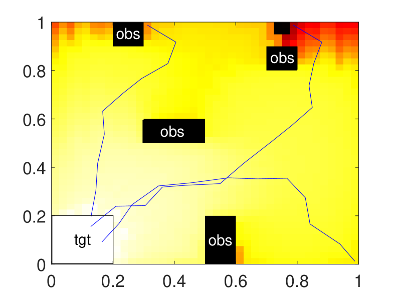
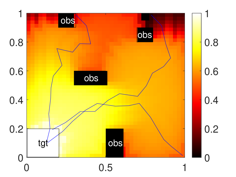
Figure 1. Results of experiments $\#1-\#3$ in Table 1. Lower bound in the probability of reachability. The plotted trajectories correspond to Monte Carlo simulations of System (7.3) taking samples from a distribution $\widetilde{p}_{v}\in\mathcal{P}_{v}$.

The lower bound on the reachability probability obtained for experiments $\#1-\#3$ (representing the different $\varepsilon$ values in Table 1) is presented in Figure 1. It is clear from the figure that the larger the ambiguity set is, the more conservative the lower bound becomes. Figure 2 shows the vector field of System (7.3) when the optimal strategy synthesized for experiment $\#1$ is applied. The synthesized strategy is almost the same for experiments $\#1-\#3$.

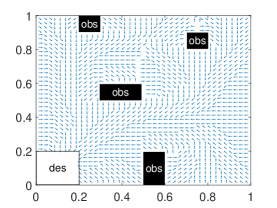
Figure 2. Vector field of System (7.3) in closed loop with the optimal strategy obtained for experiment $\#1$ in Table 1.

To compare our approach with the one that relies on IMDP abstractions described in Remark 5.3, we present the results obtained with the latter in the last row of Table 1. For this experiment, which we refer to as experiment $\#4$, the abstraction was constructed in $13$ minutes. We compare the obtained lower bounds on the reachability probability for experiments $\#1$ and $\#4$ in Figure 3, since they are obtained for the same ambiguity set for the continuous-state system. The results show how our proposed approach, despite requiring a substantially larger amount of time to perform strategy synthesis, is able to provide non-trivial satisfaction guarantees, unlike the approach from Remark 5.3. Furthermore, our approach is able to synthesize a strategy that satisfies the reachability task, in contrast to the approach based on the IMDP abstraction.

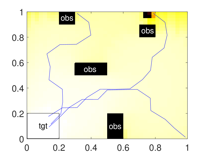
(a) Robust MDP abstraction approach

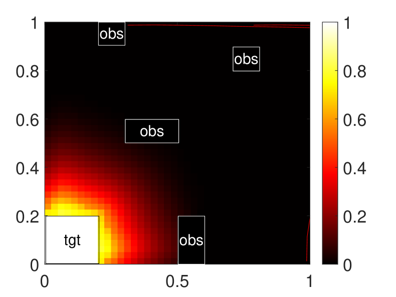
(b) IMDP abstraction approach

Figure 3. Results of experiments $\#1$ and $\#4$ in Table 1. Lower bound in the probability of reachability. The trajectories in both figures correspond to Monte Carlo simulations of System (7.3) taking samples from a distribution $\widetilde{p}_{v}\in\mathcal{P}_{v}$. The ones that satisfy the specification are presented in blue, while the ones that do not are presented in red.

7.2. Nonlinear System with 4 Modes

For the second case study we consider the nonlinear system from [23, 1] with dynamics:

$$x_{k+1}=x_{k}+\widetilde{f}_{u_{k}}(x_{k})+\textbf{v}_{k}.$$ (7.4)

Denoting by $x^{(i)}$ the $i$-th component of the state, the map $\widetilde{f}_{u_{k}}$ is given by

$$\widetilde{f}_{u}(x)=\begin{cases}[0.5+0.2\sin(x^{(2)}),0.4\cos(x^{(1)})]^{T}\qquad&\text{if}\>u=1\\ [-0.5+0.2\sin(x^{(2)}),0.4\cos(x^{(1)})]^{T}\qquad&\text{if}\>u=2\\ [0.4\cos(x^{(2)}),0.5+0.2\sin(x^{(1)})]^{T}\qquad&\text{if}\>u=3\\ [0.4\cos(x^{(2)}),-0.5+0.2\sin(x^{(1)})]^{T}\qquad&\text{if}\>u=4.\end{cases}$$ (7.5)

The system has state $x_{k}\in\mathbb{R}^{2}$ and its control input $u_{k}$ switches between the discrete values 1, 2 , 3, and 4. In analogy to the first case study, we define the safe set $X$ as the rectangle $[-2,2]\times[-2,2]\subset\mathbb{R}^{2}$ and exclude the obstacles contained therein and discretize it into a uniform grid, which results in abstraction with $N=1601$ states. The ambiguity set here is centered at an empirical distribution of $M=20$ samples, that are again drawn from a Gaussian mixture with two components, centered at $[-0.05,0]$ and $[0.05,0]$, respectively, with covariance matrix ${\rm diag}(4\times 10^{-4},4\times 10^{-4})$. Again, the centers of both components are separated by a distance close to the size of the state discretization. The results were obtained for an ambiguity radius $\varepsilon=5\times 10^{-2}$, which yield $e_{\rm{avg}}=0.25$. Furthermore, the abstraction time was around $20$ minutes, and the synthesis process took $2.43$ hours when using Linprog and $0.36$ minutes when using our dual algorithm in Section 6.3. $K_{\rm lower}=15$ iterations were performed for the case of $\underline{p}^{k}$ and $K_{\rm upper}=6$ times for the case of $\overline{p}^{k}$. The results obtained are shown in Figure 4.

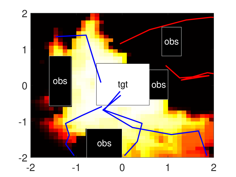
(a) Lower bound on the
    reachability probability

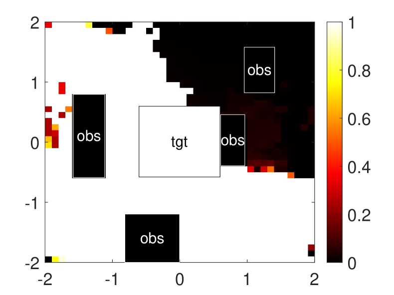
(b) Upper bound on the
    reachability probability

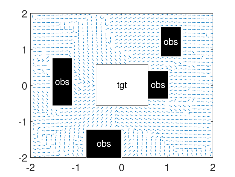
(c) Optimal strategy

Figure 4. Results obtained for the nonlinear system (7.4). The trajectories in Figure 4(a) correspond to Monte Carlo simulations of System (7.4) taking samples from a distribution $\widetilde{p}_{v}\in\mathcal{P}_{v}$. The ones that satisfy the specification are presented in blue, while the ones that do not are presented in red.

All results were obtained with an Intel Core i5-7300HQ CPU at 2.50GHz-2.50 GHz with 8GB of RAM.

8. Conclusion

In this paper we presented a framework for the formal control of switched stochastic systems with additive, random disturbances whose probability distribution belongs to a Wasserstein ambiguity set. To this end, we derived a robust MDP abstraction of the original system and proposed an algorithm, termed robust value iteration, to synthesize robust strategies that maximize the probability of satisfying a reach-avoid specification. The obtained results demonstrate the effectiveness of our approach in systems with both linear and nonlinear dynamics, and show its superiority with respect to leveraging directly IMDP abstractions.

Appendix A Proof of Proposition 5.2

To prove the proposition we will use two technical lemmas that link couplings and optimal transport discrepancies in the continuous and abstract space.

Lemma A.1 (Induced Coupling on the Discrete Space).

Consider the coupling $\pi\in\mathcal{P}(\mathbb{R}^{n}\times\mathbb{R}^{n})$ with marginals $p$ and $p^{\prime}$, a finite (measurable) partition $Q$ of $\mathbb{R}^{n}$, and the induced distributions $\gamma,\gamma^{\prime}\in\mathcal{D}(Q)$ with $\gamma(q):=p(q)$ and $\gamma^{\prime}(q):=p(q)$ for all $q\in Q$. Then $\nu\in\mathcal{P}(Q\times Q)$, defined by

$$\nu(q,q^{\prime}):=\int_{q\times q^{\prime}}d\pi(x,y)$$ (A.1)

is a coupling between $\gamma$ and $\gamma$.

Proof.

The proof follows directly from the fact that

$$\sum_{q^{\prime}\in Q}\nu(q,q^{\prime})=\sum_{q^{\prime}\in Q}\int_{q\times q^{\prime}}d\pi(x,y)=\int_{q\times\mathbb{R}^{n}}d\pi(x,y)=\gamma(q),$$

and analogously for the other marginal. ∎

Next, given two distributions on the continuous space $\mathbb{R}^{n}$ we establish bounds on the optimal transport discrepancy $\mathcal{T}_{c}$ of their induced distributions on $Q$, based on their $s$-Wasserstein distance in the continuous space.

Lemma A.2 (Induced optimal transport discrepancy).

Let $p,p^{\prime}\in\mathcal{D}_{s}(\mathbb{R}^{n})$ and consider the induced distributions $\gamma,\gamma^{\prime}\in\mathcal{D}(Q)$ with $\gamma(q):=p(q)$ and $\gamma^{\prime}(q):=p(q)$ for all $q\in Q$. Then for any $s\geq 1$ and $\varepsilon\geq 0$ it holds that

$$\mathcal{W}_{s}(p,p^{\prime})\leq\varepsilon\Rightarrow\mathcal{T}_{c}(\gamma,\gamma^{\prime})\leq\varepsilon^{s},$$

where $c$ is given in (5.4).

Proof.

Consider the map $J$ in (6.11) and note that due to (5.4),

$$\|x-y\|^{s}\geq c(J(x),J(y))$$ (A.2)

for all $x,y\in\mathbb{R}^{n}$. Let $\pi$ be an optimal coupling for the $s$-Wasserstein distance $\mathcal{W}_{s}(p,p^{\prime})$ and $\nu$ be the induced coupling on $Q$ given by (A.1). Then we get from (2.1), (6.11), and (A.2) that

$$\mathcal{W}_{s}(p,p^{\prime})^{s} =\int_{\mathbb{R}^{n}\times\mathbb{R}^{n}}\|x-y\|^{s}d\pi(x,y)\geq\int_{\mathbb{R}^{n}\times\mathbb{R}^{n}}c(J(x),J(y))d\pi(x,y)$$

$$=\sum_{q,q^{\prime}\in Q}c(q,q^{\prime})\int_{q\times q^{\prime}}d\pi(x,y)=\sum_{q,q^{\prime}\in Q}c(q,q^{\prime})\nu(q,q^{\prime})\geq\mathcal{T}_{c}(\gamma,\gamma^{\prime}),$$

which implies the result. The last inequality follows from (2.1) and Lemma A.1, which asserts that $\nu$ is a coupling between $\gamma$ and $\gamma^{\prime}$. The proof is complete. ∎

The intuition behind Lemma A.2 is the following: if the $s$-Wasserstein distance between two distributions in $\mathbb{R}^{n}$ is at most $\varepsilon$, then the optimal transport discrepancy (based on $c$) between their induced distributions on $Q$ is not more than $\varepsilon^{s}$.

Proof of Proposition 5.2.

Let $q$, $a$, $x$, and $p_{v}$ as given in the statement and define

$$\widehat{\gamma}_{x,a}(q^{\prime}):=T_{\widehat{p}_{v}}^{a}(q^{\prime}\mid x)$$

for all $q^{\prime}\in Q$. Then it follows from (5.1) and (5.3) that

$$\widehat{\gamma}_{x,a}\in\widehat{\Gamma}_{q,a}.$$ (A.3)

Next, we get from (3.2) and Assumption 3.1 that $T_{p_{v}}^{a}(\cdot\mid x)$ and $T_{\widehat{p}_{v}}^{a}(\cdot\mid x)$ are distributions in $\mathcal{D}_{s}(\mathbb{R}^{n})$ and that

$$\mathcal{W}_{s}\Big{(}T_{p_{v}}^{a}(\cdot\mid x),T_{\widehat{p}_{v}}^{a}(\cdot\mid x)\Big{)}\leq\varepsilon.$$

Since the induced distributions of $T_{p_{v}}^{a}(\cdot\mid x)$ and $T_{\widehat{p}_{v}}^{a}(\cdot\mid x)$ on $Q$ are $\gamma_{x,a}$ and $\widehat{\gamma}_{x,a}$, respectively, it follows from Lemma A.2 that $\mathcal{T}_{c}(\gamma_{x,a},\widehat{\gamma}_{x,a})\leq\varepsilon^{s}\equiv\epsilon$, namely, $\gamma_{x,a}\in\mathcal{T}_{c}^{\epsilon}(\widehat{\gamma}_{x,a})$. Thus, we deduce from (5.5) and (A.3) that $\gamma_{x,a}\in\Gamma_{q,a}$ and conclude the proof. ∎

Appendix B Proof of Theorem 6.4

Proof of Theorem 6.4.

Throughout the proof we use the shorthand notation $p_{i}\equiv\underline{p}^{k}(q_{i})$, $\underline{P}_{j}\equiv\underline{P}(q,a,q_{j})$, $\overline{P}_{j}\equiv\overline{P}(q,a,q_{j})$, $\overline{\mathcal{N}}\equiv\overline{\mathcal{N}}^{q,a}$ and $\overline{\mathcal{N}}_{W}\equiv\overline{\mathcal{N}}_{W}^{q,a}$. Concavity of $G$ follows by standard arguments from convex analysis [7]. In particular, the functions $h_{j}$ are concave as the pointwise minimum of affine functions and $\min\{\underline{P}_{j}(\lambda+h_{j}(\mu)),\overline{P}_{j}(\lambda+h_{j}(\mu))\}$ is in turn concave as the minimum of concave functions. Thus, $G$ is also concave as the sum of concave functions.

To obtain (6.9), we first eliminate $\gamma$ and $\widehat{\gamma}$ from (6.7)-(6.8) and get the equivalent problem

$$\min_{\pi_{ij}}\quad\sum_{i\in\overline{\mathcal{N}}_{W},j\in\overline{\mathcal{N}}}\pi_{ij} p_{i}$$

$$\textrm{s.t.}\quad\sum_{i\in\overline{\mathcal{N}}_{W}}\pi_{ij} \geq\underline{P}_{j} \forall j\in\overline{\mathcal{N}}$$

$$\sum_{i\in\overline{\mathcal{N}}_{W}}-\pi_{ij} \geq-\overline{P}_{j} \forall j\in\overline{\mathcal{N}}$$

$$\sum_{i\in\overline{\mathcal{N}}_{W},j\in\overline{\mathcal{N}}}-c(q_{i},q_{j})\pi_{ij} \geq-\epsilon$$

$$\sum_{i\in\overline{\mathcal{N}}_{W},j\in\overline{\mathcal{N}}}\pi_{ij} =1$$

$$\pi_{ij} \geq 0 \forall i\in\overline{\mathcal{N}}_{W},j\in\overline{\mathcal{N}}$$

By denoting $\alpha:=(\alpha_{1},\ldots,\alpha_{N})$, $\beta:=(\beta_{1},\ldots,\beta_{N})$, $\mu$, and $\lambda$ the corresponding dual variables of all but the last set of constraints, we obtain as in [3, Page 142] the dual linear problem

$$\max_{\alpha,\beta,\mu\geq 0,\lambda} \sum_{j\in\overline{\mathcal{N}}}\big{(}\alpha_{j}\underline{P}_{j}-\beta_{j}\overline{P}_{j}\big{)}-\mu\epsilon+\lambda$$

s.t. $$\alpha_{j}-\beta_{j}-\mu c(q_{i},q_{j})+\lambda\leq p_{i}\qquad\forall i\in\overline{\mathcal{N}}_{W},j\in\overline{\mathcal{N}}.$$

Since the feasible set of the primal problem is nonempty and compact, strong duality holds (cf. [3, Theorem 4.4]). The constraints of the dual problem are equivalently written

$$-\alpha_{j}+\beta_{j}+\min_{i\in\overline{\mathcal{N}}_{W}}\{p_{i}+\mu c(q_{i},q_{j})\}-\lambda\geq 0\qquad\forall j\in\overline{\mathcal{N}}$$

and since $\beta_{j}\geq 0$, they can be cast in the form

$$\beta_{j}\geq\max\{0,\alpha_{j}-\min_{i\in\overline{\mathcal{N}}_{W}}\{p_{i}+\mu c(q_{i},q_{j})\}+\lambda\}\qquad\forall j\in\overline{\mathcal{N}}.$$

Taking into account that the objective function of the dual problem is decreasing in each $\beta_{j}$, its optimal value is the same as that of the problem

$$\max_{\alpha,\mu\geq 0,\lambda}\sum_{j\in\overline{\mathcal{N}}}\big{(}\alpha_{j}\underline{P}_{j}-\max\{0,\alpha_{j}-\min_{i\in\overline{\mathcal{N}}_{W}}\{p_{i}+\mu c(q_{i},q_{j})\}+\lambda\}\overline{P}_{j}\big{)}-\mu\epsilon+\lambda$$

$$\qquad=\max_{\alpha,\mu\geq 0,\lambda}\sum_{j\in\overline{\mathcal{N}}}\big{(}\alpha_{j}\underline{P}_{j}+\min\{0,-\alpha_{j}+h_{j}(\mu)-\lambda\}\overline{P}_{j}\big{)}-\mu\epsilon+\lambda$$

$$\qquad=\max_{\alpha,\mu\geq 0,\lambda}\sum_{j\in\overline{\mathcal{N}}}\min\{\alpha_{j}\underline{P}_{j},\alpha_{j}(\underline{P}_{j}-\overline{P}_{j})+\overline{P}_{j}(h_{j}(\mu)-\lambda)\}-\mu\epsilon+\lambda,$$ (B.1)

where we used (6.10a) in the first equality. Next, since each $\overline{P}_{j}>0$, the corresponding function

$$\alpha_{j}\mapsto\varphi_{j}(\alpha_{j}):=\min\{\alpha_{j}\underline{P}_{j},\alpha_{j}(\underline{P}_{j}-\overline{P}_{j})+\overline{P}_{j}(h_{j}(\mu)-\lambda)\}$$

consists of two affine branches that intersect at $h_{j}(\mu)-\lambda$. In particular, over the left segment $\alpha_{j}\mapsto\alpha_{j}\underline{P}_{j}$ where $\alpha_{j}\leq h_{j}(\mu)-\lambda$, the slope is non-negative, and it is non-positive over the right segment $\alpha_{j}\mapsto\alpha_{j}(\underline{P}_{j}-\overline{P}_{j})+\overline{P}_{j}(h_{j}(\mu)-\lambda)$ where $\alpha_{j}\geq h_{j}(\mu)-\lambda$. Thus, the maximum of the function $\varphi_{j}$ is attained at $h_{j}(\mu)-\lambda$ when $h_{j}(\mu)-\lambda\geq 0$ and equals $(h_{j}(\mu)-\lambda)\overline{P}_{j}$, and at $0$ when $h_{j}(\mu)-\lambda<0$ where it is equal to $(h_{j}(\mu)-\lambda)\underline{P}_{j}$. Namely, we have

$$\max_{\alpha_{j}\geq 0}\varphi_{j}(\alpha_{j})=\begin{cases}(h_{j}(\mu)-\lambda)\overline{P}_{j}&{\rm if}\;h_{j}(\mu)-\lambda\geq 0\\ (h_{j}(\mu)-\lambda)\underline{P}_{j}&{\rm if}\;h_{j}(\mu)-\lambda<0\end{cases}=\min\{(h_{j}(\mu)-\lambda)\overline{P}_{j},(h_{j}(\mu)-\lambda)\underline{P}_{j}\},$$

which by virtue of (B.1) implies the dual reformulation (6.9).

To prove the last assertion of Theorem 6.4, fix an arbitrary value of $\mu\geq 0$ and consider the function $\lambda\mapsto G_{\mu}(\lambda)\equiv G(\lambda,\mu)$ with $G$ as given in (6.9). Notice that each $\min$ term in the expression of $G_{\mu}$ is a piecewise affine function of $\lambda$ with two segments and a breakpoint at $h_{j}(\mu)$ (assuming without loss of generality that $\underline{P}_{j}\neq\overline{P}_{j}$). Since $G_{\mu}$ is the sum of piecewise affine functions, it is also piecewise affine and its breakpoints are included in the breakpoints of its components, i.e., in the set $\{h_{j}(\mu)\}_{j\in\overline{\mathcal{N}}}$. Taking further into account that $G_{\mu}$ is upper bounded by the optimal value of problem (6.9)-(6.10), which is finite by strong duality, its maximum is necessarily attained at some of its breakpoints. This concludes the proof. ∎

References

- [1] S. Adams, M. Lahijanian, and L. Laurenti, “Formal control synthesis for stochastic neural network dynamic models,” IEEE Control Systems Letters, 2022.
- [2] D. P. Bertsekas and S. Shreve, Stochastic optimal control: the discrete-time case, 2004.
- [3] D. Bertsimas and J. N. Tsitsiklis, Introduction to linear optimization. Athena scientific, 1997, vol. 6.
- [4] J. Blanchet and K. Murthy, “Quantifying distributional model risk via optimal transport,” Mathematics of Operations Research, vol. 44, no. 2, pp. 565–600, 2019.
- [5] J. Blanchet, K. Murthy, and F. Zhang, “Optimal transport-based distributionally robust optimization: Structural properties and iterative schemes,” Mathematics of Operations Research, vol. 47, no. 2, pp. 1500–1529, 2022.
- [6] D. Boskos, J. Cortés, and S. Martínez, “High-confidence data-driven ambiguity sets for time-varying linear systems,” IEEE Transactions on Automatic Control, 2023.
- [7] S. Boyd and L. Vandenberghe, Convex optimization. Cambridge university press, 2004.
- [8] G. C. Calafiore and L. E. Ghaoui, “On distributionally robust chance-constrained linear programs,” Journal of Optimization Theory and Applications, vol. 130, no. 1, pp. 1–22, 2006.
- [9] N. Cauchi, L. Laurenti, M. Lahijanian, A. Abate, M. Kwiatkowska, and L. Cardelli, “Efficiency through uncertainty: Scalable formal synthesis for stochastic hybrid systems,” in Proceedings of the 2019 22nd ACM International Conference on Hybrid Systems: Computation and Control. Montreal, QC, Canada: ACM, Apr. 2019.
- [10] J. G. Clement and C. Kroer, “First-order methods for wasserstein distributionally robust mdp,” in International Conference on Machine Learning. PMLR, 2021, pp. 2010–2019.
- [11] E. Delage and Y. Ye, “Distributionally robust optimization under moment uncertainty with application to data-driven problems,” Operations research, vol. 58, no. 3, pp. 595–612, 2010.
- [12] M. Dutreix and S. Coogan, “Specification-guided verification and abstraction refinement of mixed monotone stochastic systems,” IEEE Transactions on Automatic Control, vol. 66, no. 7, pp. 2975–2990, 2020.
- [13] M. Dutreix, J. Huh, and S. Coogan, “Abstraction-based synthesis for stochastic systems with omega-regular objectives,” Nonlinear Analysis: Hybrid Systems, vol. 45, p. 101204, 2022.
- [14] L. El Ghaoui and A. Nilim, “Robust solutions to markov decision problems with uncertain transition matrices,” Operations Research, vol. 53, no. 5, pp. 780–798, 2005.
- [15] N. Fournier and A. Guillin, “On the rate of convergence in wasserstein distance of the empirical measure,” Probability Theory and Related Fields, vol. 162, no. 3, pp. 707–738, 2015.
- [16] R. Gao and A. Kleywegt, “Distributionally robust stochastic optimization with wasserstein distance,” Mathematics of Operations Research, 2022.
- [17] R. Givan, S. Leach, and T. Dean, “Bounded-parameter Markov decision processes,” Artificial Intelligence, vol. 122, no. 1-2, pp. 71–109, 2000.
- [18] I. Gracia, D. Boskos, L. Laurenti, and M. Mazo Jr, “Distributionally robust strategy synthesis for switched stochastic systems,” in Proceedings of the 26th ACM International Conference on Hybrid Systems: Computation and Control, 2023, pp. 1–10.
- [19] S. Haesaert, N. Cauchi, and A. Abate, “Certified policy synthesis for general Markov decision processes: An application in building automation systems,” Performance Evaluation, vol. 117, pp. 75–103, 2017.
- [20] A. Hakobyan and I. Yang, “Wasserstein distributionally robust motion control for collision avoidance using conditional value-at-risk,” IEEE Transactions on Robotics, vol. 38, no. 2, pp. 939–957, 2021.
- [21] G. N. Iyengar, “Robust dynamic programming,” Mathematics of Operations Research, vol. 30, no. 2, pp. 257–280, 2005.
- [22] J. Jackson, L. Laurenti, E. Frew, and M. Lahijanian, “Formal verification of unknown dynamical systems via gaussian process regression,” arXiv preprint arXiv:2201.00655, 2021.
- [23] ——, “Strategy synthesis for partially-known switched stochastic systems,” in Proceedings of the 24th International Conference on Hybrid Systems: Computation and Control, 2021, pp. 1–11.
- [24] X. Koutsoukos and D. Riley, “Computational methods for reachability analysis of stochastic hybrid systems,” in International Workshop on Hybrid Systems: Computation and Control. Springer, 2006, pp. 377–391.
- [25] M. Lahijanian, S. B. Andersson, and C. Belta, “Formal verification and synthesis for discrete-time stochastic systems,” IEEE Transactions on Automatic Control, vol. 60, no. 8, pp. 2031–2045, 2015.
- [26] L. Laurenti, M. Lahijanian, A. Abate, L. Cardelli, and M. Kwiatkowska, “Formal and efficient synthesis for continuous-time linear stochastic hybrid processes,” IEEE Transactions on Automatic Control, vol. 66, no. 1, pp. 17–32, 2020.
- [27] A. Lavaei and M. Zamani, “From dissipativity theory to compositional synthesis of large-scale stochastic switched systems,” IEEE Transactions on Automatic Control, 2022.
- [28] R. Luna, M. Lahijanian, M. Moll, and L. E. Kavraki, “Asymptotically optimal stochastic motion planning with temporal goals,” in Algorithmic Foundations of Robotics XI. Springer, 2015, pp. 335–352.
- [29] P. Mohajerin Esfahani and D. Kuhn, “Data-driven distributionally robust optimization using the wasserstein metric: Performance guarantees and tractable reformulations,” Mathematical Programming, vol. 171, no. 1, pp. 115–166, 2018.
- [30] A. Nilim and L. El Ghaoui, “Robust control of markov decision processes with uncertain transition matrices,” Operations Research, vol. 53, no. 5, pp. 780–798, 2005.
- [31] I. Popescu, “Robust mean-covariance solutions for stochastic optimization,” Operations Research, vol. 55, no. 1, pp. 98–112, 2007.
- [32] A. Puggelli, W. Li, A. L. Sangiovanni-Vincentelli, and S. A. Seshia, “Polynomial-time verification of pctl properties of mdps with convex uncertainties,” in International Conference on Computer Aided Verification. Springer, 2013, pp. 527–542.
- [33] H. Rahimian and S. Mehrotra, “Distributionally robust optimization: A review,” arXiv preprint arXiv:1908.05659, 2019.
- [34] S. Ramani and A. Ghate, “Robust markov decision processes with data-driven, distance-based ambiguity sets,” SIAM Journal on Optimization, vol. 32, no. 2, pp. 989–1017, 2022.
- [35] F. Santambrogio, “Optimal transport for applied mathematicians,” Birkäuser, NY, vol. 55, no. 58-63, p. 94, 2015.
- [36] C. Santoyo, M. Dutreix, and S. Coogan, “A barrier function approach to finite-time stochastic system verification and control,” Automatica, vol. 125, p. 109439, 2021.
- [37] A. Shapiro, “Distributionally robust stochastic programming,” SIAM Journal on Optimization, vol. 27, no. 4, pp. 2258–2275, 2017.
- [38] P. Tabuada, “An approximate simulation approach to symbolic control,” IEEE Transactions on Automatic Control, vol. 53, no. 6, pp. 1406–1418, 2008.
- [39] C. Villani, Topics in optimal transportation. American Mathematical Society, 2003, vol. 58.
- [40] W. Wiesemann, D. Kuhn, and B. Rustem, “Robust markov decision processes,” Mathematics of Operations Research, vol. 38, no. 1, pp. 153–183, 2013.
- [41] E. M. Wolff, U. Topcu, and R. M. Murray, “Robust control of uncertain markov decision processes with temporal logic specifications,” in 2012 IEEE 51st IEEE Conference on Decision and Control (CDC). IEEE, 2012, pp. 3372–3379.
- [42] H. Xu and S. Mannor, “Distributionally robust markov decision processes,” Advances in Neural Information Processing Systems, vol. 23, 2010.
- [43] I. Yang, “A convex optimization approach to distributionally robust markov decision processes with wasserstein distance,” IEEE control systems letters, vol. 1, no. 1, pp. 164–169, 2017.
- [44] G. Yin and C. Zhu, Hybrid switching diffusions: properties and applications. Springer New York, 2010, vol. 63.