Elastic anisotropy in heterogeneous materials

Abstract

Heterogeneous materials exhibit anisotropy to varying extent that is influenced by factors such as individual phase properties and microstructural configuration. A review of the existing anisotropy measures proposed in the context of single crystals reveal that they do not account for the material and microstructural descriptors influencing the extent of anisotropy in heterogeneous materials. To overcome this limitation, existing anisotropy indices have been re-interpreted by considering the effective elastic properties of heterogeneous materials obtained by appropriate homogenization techniques. Anisotropy quantification has been demonstrated considering two phase composite materials highlighting the role of constituent volume fractions, secondary phase shape and elastic contrast in influencing the extent of anisotropy. Specific cases leading to overall isotropy in two phase composite materials and extension of the approach to consider porosity and cracks have also been presented demonstrating the applicability of the approach to any class of heterogeneous materials thus filling a crucial gap in the existing literature.

I Introduction

Anisotropy, defined as the direction dependence of material response, is a key aspect characterizing material behavior. Various classes of natural and engineered materials such as single crystals [1], polycrystals [2], composite materials [3], biological tissues [4, 5], geological materials [6], 2D materials [7] etc. exhibit mechanical anisotropy to varying degree. Additionally, anisotropy plays an important role in phenomena such as phase transformations [8], material damage [9], dislocation dynamics [10], defect mobility [11], fracture behavior [12], plastic deformation in crystals [13] etc. The pervasive nature of anisotropy illustrates the importance of quantifying it by relevant measures.

Elastic anisotropy type can be represented graphically [14, 15] and by material symmetry groups [16]. However, a quantifiable parameter in the form of a scalar anisotropy index facilitates the comparison of the extent of anisotropy within and across material symmetry groups. The extent of elastic anisotropy can be determined from the elastic behavior of materials represented by generalized Hooke’s law ($\sigma_{ij}=C_{ijkl}\epsilon_{kl}$) consisting of a fourth-rank elastic stiffness tensor ($C_{ijkl}$) relating the second rank stress ($\sigma_{ij}$) and strain ($\epsilon_{kl}$) tensors. The generalized Hooke’s law can be represented in matrix form through Voigt contraction in the following form that has formed the basis for anisotropy quantification so far.

$${\begin{bmatrix}\sigma_{11}\\ \sigma_{22}\\ \sigma_{33}\\ \sigma_{23}\\ \sigma_{13}\\ \sigma_{12}\\ \end{bmatrix}=\begin{bmatrix}C_{11}&C_{12}&C_{13}&C_{14}&C_{15}&C_{16}\\ C_{21}&C_{22}&C_{23}&C_{24}&C_{25}&C_{26}\\ C_{31}&C_{32}&C_{33}&C_{34}&C_{35}&C_{36}\\ C_{41}&C_{42}&C_{43}&C_{44}&C_{45}&C_{46}\\ C_{51}&C_{52}&C_{53}&C_{54}&C_{55}&C_{56}\\ C_{61}&C_{62}&C_{63}&C_{64}&C_{65}&C_{66}\\ \end{bmatrix}\begin{bmatrix}\epsilon_{11}\\ \epsilon_{22}\\ \epsilon_{33}\\ 2\epsilon_{23}\\ 2\epsilon_{13}\\ 2\epsilon_{12}\\ \end{bmatrix}}$$ (1)

In addition to anisotropy, certain classes of materials mentioned above such as composite materials, biological tissues, geological materials etc. also exhibit spatial variation of mechanical properties termed as heterogeneity. In contrast to homogeneous materials, the elastic stiffness of a heterogeneous material is a function of spatial location within the material i.e. $C_{ijkl}=C_{ijkl}(x,y,z)$ where $x,y,z\in\mathbb{R}^{3}$ denote spatial co-ordinates within the material. While anisotropy quantification in single crystals has received enough attention and is directly applicable in the case of homogeneous materials, similar quantification for heterogeneous material accounting for the spatial variation of elastic stiffness is currently lacking that forms the focus of the current work.

II Single crystal anisotropy indices

Anisotropy quantification in single crystals has been explored by a diverse range of anisotropy indices. Zener’s anisotropy index $A^{Z}=2C_{44}/(C_{11}-C_{12})$, where $C_{11}$, $C_{12}$, and $C_{44}$ are the independent single crystal elastic constants [17], quantifies anisotropy as the ratio of the extreme values of orientation dependent shear moduli that is valid for crystals with cubic symmetry. $A^{Z}$ measures anisotropy as deviation from unity which indicates isotropy and is ambiguous since values both lower and higher than unity indicate anisotropy leading to a lack of universality.

Chung and Buessem [18] proposed a measure of anisotropy based on the equality of shear moduli obtained from Voigt ($\mu^{V}$) and Reuss average ($\mu^{R}$) of shear modulus leading to an anisotropy index in the form $A^{C}=(\mu^{V}-\mu^{R})/(\mu^{V}+\mu^{R})$. Although $A^{C}$ can be calculated for any crystal symmetry, disregarding the bulk modulus which influences anisotropy of crystals other those exhibiting cubic symmetry reduces it’s utility in crystals with lower symmetries. Ledbetter and Migliori [19] proposed a more general anisotropy index based on shear wave velocities in the form $A^{*}=\nu_{2}^{2}/\nu_{1}^{2}$ where $\nu_{1}$ and $\nu_{2}$ are the minimum and maximum shear sound-wave velocities among all propagation and polarization directions respectively.

The above mentioned anisotropy measures lack universality that stems from disregarding the tensorial nature of elastic stiffness as highlighted by Ranganathan & Ostoja-Starzewski [20]. The implication of disregarding the tensorial nature of the elastic stiffness is that the bulk part of the stiffness tensor is neglected limiting the utility of the above anisotropy indices to crystals with isotropic bulk resistance. Anisotropy quantification considering the tensorial nature of elastic stiffness has been attempted via tensor norm based measures by Nye [21], Zheng [22] ($A_{Nye-Zheng}=\left\|C-C^{iso}\right\|/\left\|C\right\|$, where $C-C^{iso}$ is the anisotropic part of C), Zhang [23], Rychlewski [24] ($A_{Zhang-Rychlewski}=\max\left\|R*C-C\right\|/(2\left\|C\right\|)$, where $R$ represents a rotation operation). In both the norm based measures, $\left\|C\right\|$ is the norm of a general fourth-rank tensor $C$ denoted as $\left\|C\right\|=(C_{ijkl}C_{ijkl})^{1/2}$.

A set of criteria for generality, universality, and applicability of an anisotropy index has been proposed by Fang et al. [25] that can be summarized as follows. An acceptable anisotropy index must (a) be zero in the case of isotropy with any positive number indicating anisotropy, (b) should approach infinity if there exists a direction along which the deformation resistance of the material approaches zero, and (c) must have a clear physical meaning. Of the anisotropy indices discussed previously, $A^{Z}$ and $A^{*}$ do not consider the tensorial nature of the elastic stiffness tensor and do not fulfill the first criteria for an acceptable anisotropy index. $A^{C}$ and the tensor norm based measures $A_{Nye-Zheng}$ and $A_{Zhang-Rychlewski}$ do not approach infinity if there exists a direction along which the deformation resistance of the material approaches zero thereby not satisfying the second criterion. These observations highlight the inadequacies of the discussed anisotropy indices.

In the backdrop of the inadequacies of the above anisotropy indices, the following measures seem to be acceptable indices and have been predominantly used in anisotropy quantification in single crystals.

(a) Universal anisotropy index $A^{U}$ that considers the tensorial nature of the stiffness tensor by relating anisotropy to the Euclidean distance between the Voigt ($C^{V}$) and Reuss bounds ($C^{R}$) on spatially uniformly distributed aggregate of a single crystal [20]. $A^{U}$ is a scalar that can be expressed in terms of bulk ($\kappa$) and shear moduli ($\mu$) in the following form.

$$A^{U}(C^{V},C^{R})=\frac{\kappa^{V}}{\kappa^{R}}+5\frac{\mu^{V}}{\mu^{R}}-6$$ (2)

Superscript $V$ and $R$ represent the Voigt and Reuss bounds obtained by ensemble average of randomly oriented crystals. Isotropic crystals have $A^{U}=0$ and any deviation from zero indicates anisotropy. The limitation of $A^{U}$ is that it is a relative measure of anisotropy.

(b) The relative nature of $A^{U}$ can be overcome by considering the log-Euclidean distance between the Voigt and Reuss bounds leading to an absolute anisotropy index $A^{L}$ in the following form [26].

$$A^{L}(C^{V},C^{R})=\sqrt{\left[ln\left(\frac{\kappa^{V}}{\kappa^{R}}\right)\right]^{2}+5\left[ln\left(\frac{\mu^{V}}{\mu^{R}}\right)\right]^{2}}$$ (3)

$A^{L}$ becomes zero for isotropic crystals and any deviation for zero indicates the extent of anisotropy that is valid for any crystal class. Additionally, $A^{L}$ being an absolute measure of anisotropy, the degree of anisotropy is comparable across crystals.

(c) Elastic strain energy based anisotropy index $A^{SE}$ defined as the ratio of maximum and minimum elastic strain energy across the possible range of strain combinations and crystal orientations [25].

$$A^{SE}=\max_{\epsilon,R_{\epsilon}^{(1)},R_{\epsilon}^{(2)}}\left(\frac{(R_{\epsilon}^{(1)}\epsilon)^{T}C(R_{\epsilon}^{(1)}\epsilon)}{(R_{\epsilon}^{(2)}\epsilon)^{T}C(R_{\epsilon}^{(2)}\epsilon)}\right)-1$$ (4)

Where $R_{\epsilon}$ is the rotation matrix of strain, $\epsilon$ is the strain tensor and $C$ is the stiffness tensor. $A^{SE}$ can be expressed in stress or strain space that are equivalent [25].

The terms $\kappa^{V}$, $\kappa^{R}$, $\mu^{V}$ and $\mu^{R}$ in Eq. 2, 3 are given in terms of the components of the elastic stiffness ($C_{ij}$) and compliance ($S_{ij}$) matrices of any arbitrary material in Voigt representation in the following form [27].

$$9\kappa^{V}= \left(C_{11}+C_{22}+C_{33}\right)+2\left(C_{12}+C_{13}+C_{23}\right)$$ (5)

$$15\mu^{V}= \left(C_{11}+C_{22}+C_{33}\right)-\left(C_{12}+C_{13}+C_{23}\right)$$

$$+3\left(C_{44}+C_{55}+C_{66}\right)$$

$$1/\kappa^{R}= S_{11}+S_{22}+S_{33}+2\left(S_{12}+S_{13}+S_{23}\right)$$

$$15/\mu^{R}= 4(S_{11}+S_{22}+S_{33}-S_{12}-S_{13}-S_{23})$$

$$+3(S_{44}+S_{55}+S_{66})$$

Although $A^{U}$ and $A^{L}$ satisfy the first two criteria for an acceptable anisotropy index, they relate anisotropy to the distance between Voigt and Reuss bounds (that converge when a material is isotropic) making their physical meaning difficult to comprehend. On the other hand, $A^{SE}$ relates anisotropy to strain energy satisfying the criteria for a clear physical meaning. However, taken in their proposed form, $A^{U}$, $A^{L}$ and $A^{SE}$ are strictly applicable to single crystals. While the elastic stiffness tensor of a specific single crystal with a particular crystal structure is unique, elastic stiffness tensor of a heterogeneous material is a function of the elastic properties of the constituent phases and microstructural configuration. This dependence highlights the need to critically evaluate and re-examine the applicability of these anisotropy indices in the context of heterogeneous materials considering the parameters that influence their overall elastic properties.

III Anisotropy quantification in heterogeneous materials

The effective elastic stiffness of heterogeneous materials are dependent on the constituent phase properties, relative content and microstructural configuration. Hill bounds [27] discussed in the case of single crystals while determining $A^{U}$ and $A^{L}$ take a different context in the case of heterogeneous materials [28]. Determination of $A^{U}$ and $A^{L}$ proceeds by considering all possible orientations of a single crystal with uniform probability and ensemble averaging leading to isotropic single crystal response. However, heterogeneous materials consist of two or more distinct phases and Hill bounds considering the individual phase properties provide the absolute bounds on the effective elastic properties [28]. The implication is that $A^{U}$ and $A^{L}$ taken in their proposed form (Eq.2,3) considering individual phase properties provide the maximum possible extent of anisotropy but not the actual extent of anisotropy. Consequently, anisotropy measures based on the distance between Voigt and Reuss bounds proposed in the context of single crystals needs to be suitably modified to be applicable for heterogeneous materials.

A more rigorous approach for anisotropy quantification in a heterogeneous material involves the evaluation of its effective elastic properties followed by anisotropy quantification considering the determined effective elastic properties. The effective elastic stiffness of a heterogeneous material can be obtained by homogenization which is the representation of a heterogeneous material by a equivalently homogeneous material considering individual phase elastic properties and microstructural descriptors (See Fig. 1). The effective elastic stiffness tensor $C^{*}$ of a heterogeneous material can be expressed in terms of volume averaged stress ($\bar{\sigma}$) and strain ($\bar{\epsilon}$) in the constituent phases of a heterogeneous material in the following form.

$$\bar{\sigma}=C^{*}\bar{\epsilon}$$ (6)

The effective elastic stiffness $C^{*}$ of a heterogeneous material can be obtained from a diverse range of analytical and numerical homogenization approaches [29]. With the determination of $C^{*}$, the extent of anisotropy can be quantified by distance based as well as strain energy based anisotropy criteria considering $C^{*}$ instead of the individual phase properties. Anisotropy quantification in polycrystals [30] and architectured materials [31] following a similar approach has been demonstrated previously and the present approach is a generalization that is independent of microstructural configuration and homogenization method thereby being applicable for any class of heterogeneous material.

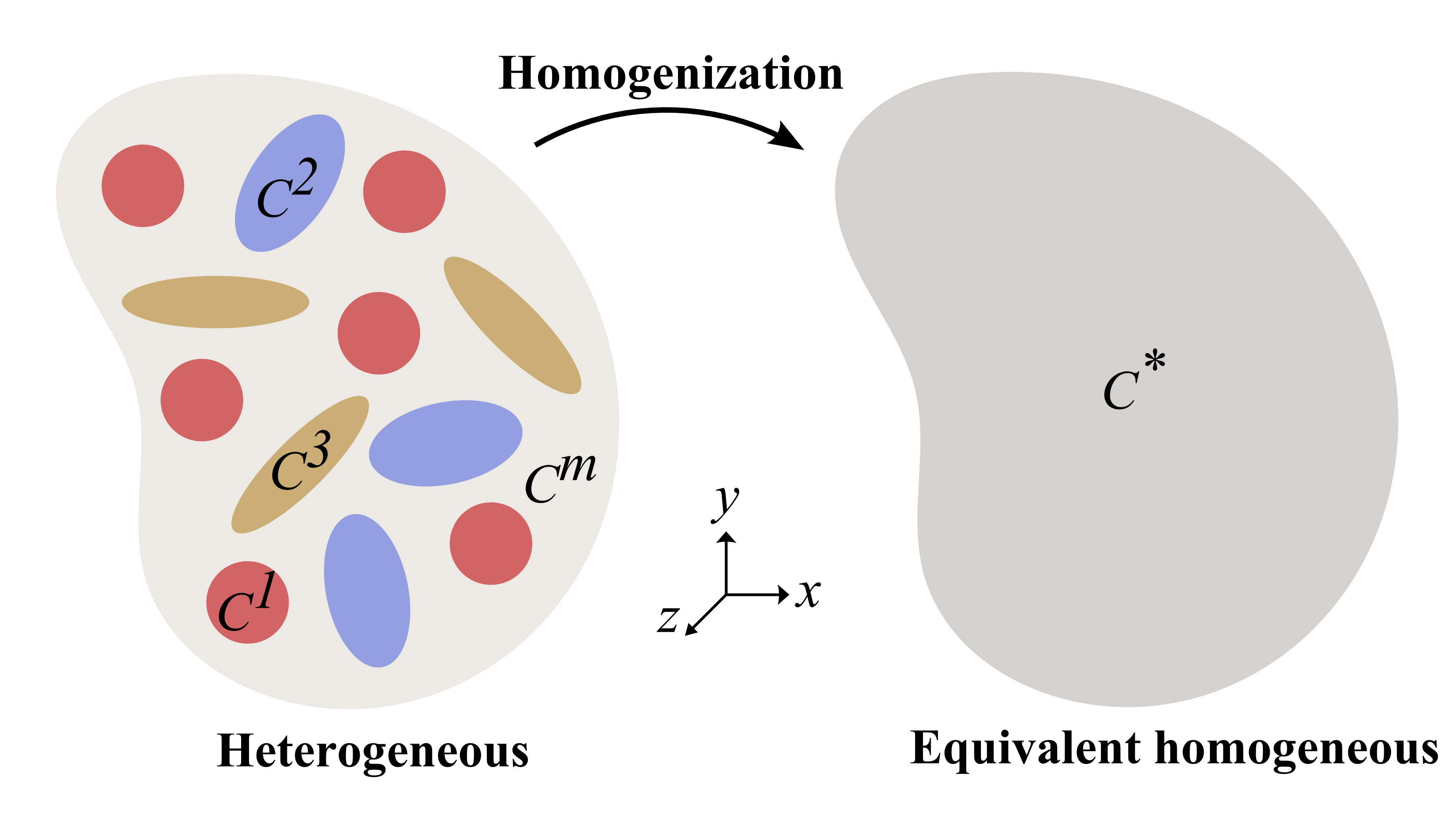
Figure 1: Schematic of homogenization representing the evaluation of the effective elastic stiffness $C^{*}$ of a heterogeneous material consisting of individual phases (with elastic stiffness $C^{1}$, $C^{2}$ etc.) embedded in a matrix with elastic stiffness $C^{m}$.

The effective elastic stiffness $C^{*}$ represents the elastic stiffness of a homogeneous material that is equivalent to the heterogeneous material under consideration without any restriction on anisotropy. Therefore, the terms in Eq. 2, 3 can be replaced with respective starred terms denoting components of the effective elastic stiffness ($C^{*}$) and compliance ($S^{*}=C^{*-1}$) matrix in the Voigt representation following Hill [27].

The modified expressions for $A^{U}$ (Eq. 2) and $A^{L}$ (Eq. 3) replacing the terms $\kappa^{V}$, $\kappa^{R}$, $\mu^{V}$ and $\mu^{R}$ with respective starred terms $\kappa^{V*}$, $\kappa^{R*}$, $\mu^{V*}$ and $\mu^{R*}$ that reflect their evaluation from $C^{*}$ and $S^{*}$ are as follows.

$$A^{U*}=\frac{\kappa^{V*}}{\kappa^{R*}}+5\frac{\mu^{V*}}{\mu^{R*}}-6$$ (7)

$$A^{L*}=\sqrt{\left[ln\left(\frac{\kappa^{V*}}{\kappa^{R*}}\right)\right]^{2}+5\left[ln\left(\frac{\mu^{V*}}{\mu^{R*}}\right)\right]^{2}}$$ (8)

Where the terms $\kappa^{V*}$, $\kappa^{R*}$, $\mu^{V*}$ and $\mu^{R*}$ are given in terms of the components of effective elastic stiffness ($C_{ij}^{*}$) and compliance ($S_{ij}^{*}$) tensors of a heterogeneous material in Voigt representation in the following form.

$$9\kappa^{V*}= \left(C_{11}^{*}+C_{22}^{*}+C_{33}^{*}\right)+2\left(C_{12}^{*}+C_{13}^{*}+C_{23}^{*}\right)$$ (9)

$$15\mu^{V*}= \left(C_{11}^{*}+C_{22}^{*}+C_{33}^{*}\right)-\left(C_{12}^{*}+C_{13}^{*}+C_{23}^{*}\right)$$

$$+3\left(C_{44}^{*}+C_{55}^{*}+C_{66}^{*}\right)$$

$$1/\kappa^{R*}= S_{11}^{*}+S_{22}^{*}+S_{33}^{*}+2\left(S_{12}^{*}+S_{13}^{*}+S_{23}^{*}\right)$$

$$15/\mu^{R*}= 4(S_{11}^{*}+S_{22}^{*}+S_{33}^{*}-S_{12}^{*}-S_{13}^{*}-S_{23}^{*})$$

$$+3(S_{44}^{*}+S_{55}^{*}+S_{66}^{*})$$

A general form of $A^{SE}$ in terms of the ratio of strain energy $U$ which is a function of orientation $R$ and applied strain $\epsilon$ is given in the following form [25].

$$A^{SE}=\max_{\epsilon,R^{(1)},R^{(2)}}\left(\frac{U(\epsilon,R^{(1)})}{U(\epsilon,R^{(2)})}\right)-1$$ (10)

The scalar strain energy $U=\sigma_{ij}\epsilon_{ij}/2$ is a function of the stress and strain tensors evaluating which involves tensorial operations. Rotation operation in Voigt notation is not consistent since the rotation matrices in stress ($R_{\sigma}$) and strain ($R_{\epsilon}$) spaces are different with both not satisfying the orthogonality relation ($R_{\sigma}R_{\sigma}^{T}\neq I$,$R_{\epsilon}R_{\epsilon}^{T}\neq I$). The rotation matrices of strain and stress can be made consistent by using isomorphism between second-rank tensors and six-dimensional vectors as well as between fourth-rank elasticity tensors and six-dimensional positive-definite symmetric matrices. The strain and stress tensors can be represented in the isomorphic form ($\tilde{\epsilon}$, $\tilde{\sigma}$) in the following form [32].

$$\tilde{\epsilon}=\begin{Bmatrix}\epsilon_{11}\\ \epsilon_{22}\\ \epsilon_{33}\\ \sqrt{2}\epsilon_{23}\\ \sqrt{2}\epsilon_{13}\\ \sqrt{2}\epsilon_{12}\\ \end{Bmatrix};\tilde{\sigma}=\begin{Bmatrix}\sigma_{11}\\ \sigma_{22}\\ \sigma_{33}\\ \sqrt{2}\sigma_{23}\\ \sqrt{2}\sigma_{13}\\ \sqrt{2}\sigma_{12}\\ \end{Bmatrix}$$ (11)

The elastic stiffness tensor in Voigt notation ($C$) can be represented in the isomorphic form ($\tilde{C}$) in the following form [32].

$$\tilde{C}=\begin{bmatrix}C_{11}&C_{12}&C_{13}&\sqrt{2}C_{14}&\sqrt{2}C_{15}&\sqrt{2}C_{16}\\ &C_{22}&C_{23}&\sqrt{2}C_{24}&\sqrt{2}C_{25}&\sqrt{2}C_{26}\\ &&C_{33}&\sqrt{2}C_{34}&\sqrt{2}C_{35}&\sqrt{2}C_{36}\\ &&&2C_{44}&2C_{45}&2C_{46}\\ &sym&&&2C_{55}&2C_{56}\\ &&&&&2C_{66}\\ \end{bmatrix}$$ (12)

The isomorphic representation of the terms in the generalized Hooke’s law retains it’s representation i.e. $\tilde{\sigma}=\tilde{C}\tilde{\epsilon}$ as well as the expression for elastic strain energy.

Rotation of $\tilde{\epsilon}$ , $\tilde{\sigma}$ and $\tilde{C}$ can be accomplished by the modified rotation matrix $\tilde{R}$ [32, 33]) that consists of directional cosines $Q_{ij}=cos(x_{i}^{\prime},x_{j})$ $i,j=1,2,3$ and satisfies the orthogonality relation in the following form.

$$\tilde{R}=\begin{bmatrix}Q_{11}^{2}&Q_{12}^{2}&Q_{13}^{2}&\sqrt{2}Q_{12}Q_{13}&\sqrt{2}Q_{11}Q_{13}&\sqrt{2}Q_{11}Q_{12}\\ Q_{21}^{2}&Q_{22}^{2}&Q_{23}^{2}&\sqrt{2}Q_{22}Q_{23}&\sqrt{2}Q_{21}Q_{23}&\sqrt{2}Q_{21}Q_{22}\\ Q_{31}^{2}&Q_{32}^{2}&Q_{33}^{2}&\sqrt{2}Q_{32}Q_{33}&\sqrt{2}Q_{31}Q_{33}&\sqrt{2}Q_{31}Q_{32}\\ \sqrt{2}Q_{21}Q_{31}&\sqrt{2}Q_{22}Q_{32}&\sqrt{2}Q_{23}Q_{33}&Q_{22}Q_{33}+Q_{23}Q_{32}&Q_{21}Q_{33}+Q_{23}Q_{31}&Q_{21}Q_{32}+Q_{22}Q_{31}\\ \sqrt{2}Q_{11}Q_{31}&\sqrt{2}Q_{12}Q_{32}&\sqrt{2}Q_{13}Q_{33}&Q_{12}Q_{33}+Q_{13}Q_{32}&Q_{11}Q_{33}+Q_{13}Q_{31}&Q_{11}Q_{32}+Q_{12}Q_{31}\\ \sqrt{2}Q_{11}Q_{21}&\sqrt{2}Q_{12}Q_{22}&\sqrt{2}Q_{13}Q_{23}&Q_{12}Q_{23}+Q_{13}Q_{22}&Q_{11}Q_{23}+Q_{13}Q_{21}&Q_{11}Q_{22}+Q_{12}Q_{21}\\ \end{bmatrix}$$ (13)

With the isomorphic representation of generalized Hooke’s law and expressions for co-ordinate transformation, the strain energy based anisotropy index in strain space for heterogeneous materials is given by the following expression

$$A^{SE*}=\max_{\epsilon,\tilde{R}^{(1)},\tilde{R}^{(2)}}\left(\frac{(\tilde{R}^{(1)}\epsilon)^{T}\tilde{C^{*}}(\tilde{R}^{(1)}\epsilon)}{(\tilde{R}^{(2)}\epsilon)^{T}\tilde{C^{*}}(\tilde{R}^{(2)}\epsilon)}\right)-1$$ (14)

where $\tilde{R}^{(1)}$ and $\tilde{R}^{(2)}$ represents the rotation matrices for distinct orientations. Detailed derivation of the strain energy based anisotropy index has been presented in the supplementary material.

$A^{U*}$ and $A^{L*}$ form the distance based anisotropy indices applicable for heterogeneous materials. $A^{U*}$ and $A^{L*}$ can be evaluated by Eq 7-9. The strain energy based anisotropy index $A^{SE*}$ needs to be evaluated by suitable optimization technique. Details of the numerical approach to evaluate $A^{U}$, $A^{L}$ and $A^{SE}$, validation with results in current literature and their extension to heterogeneous materials have been presented in the supplementary material.

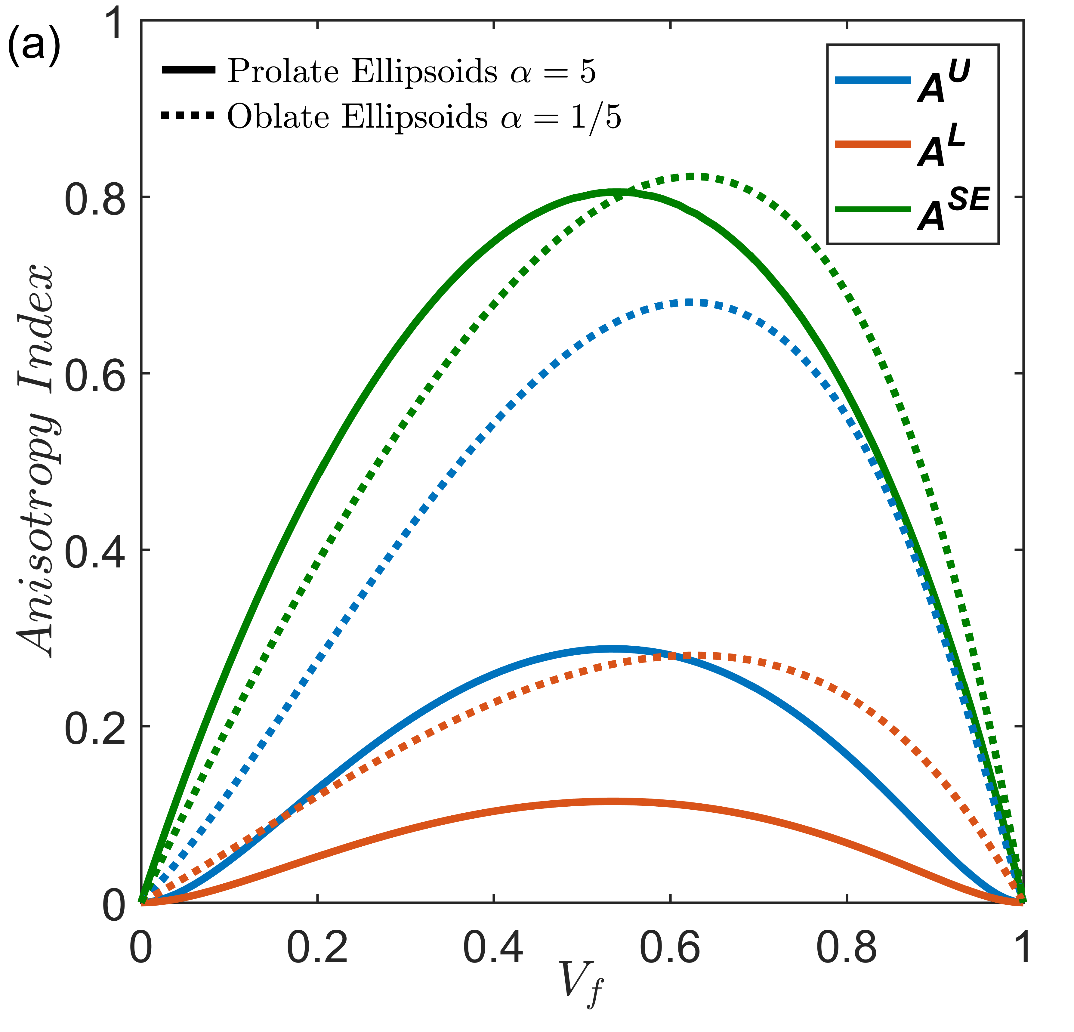
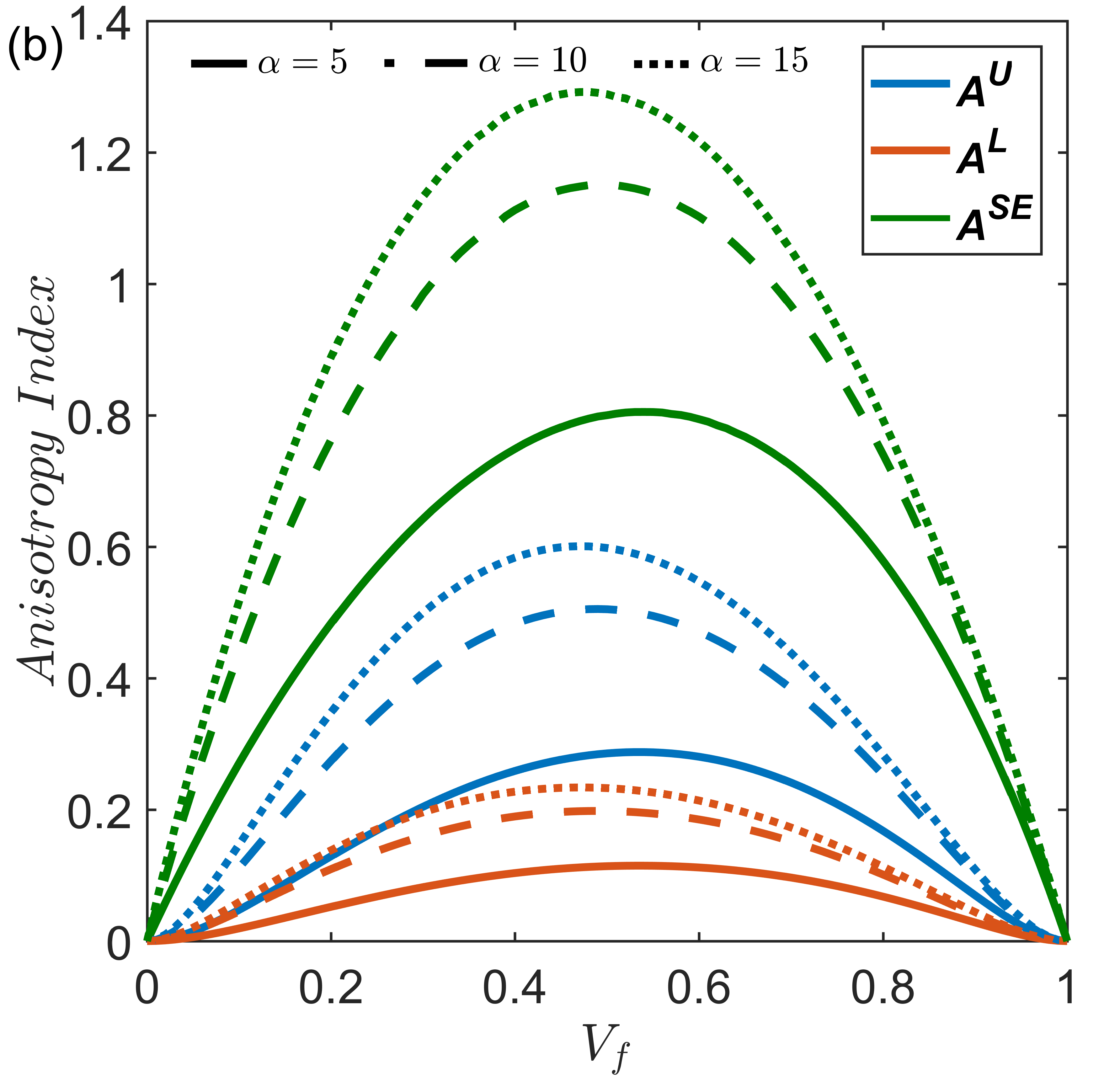
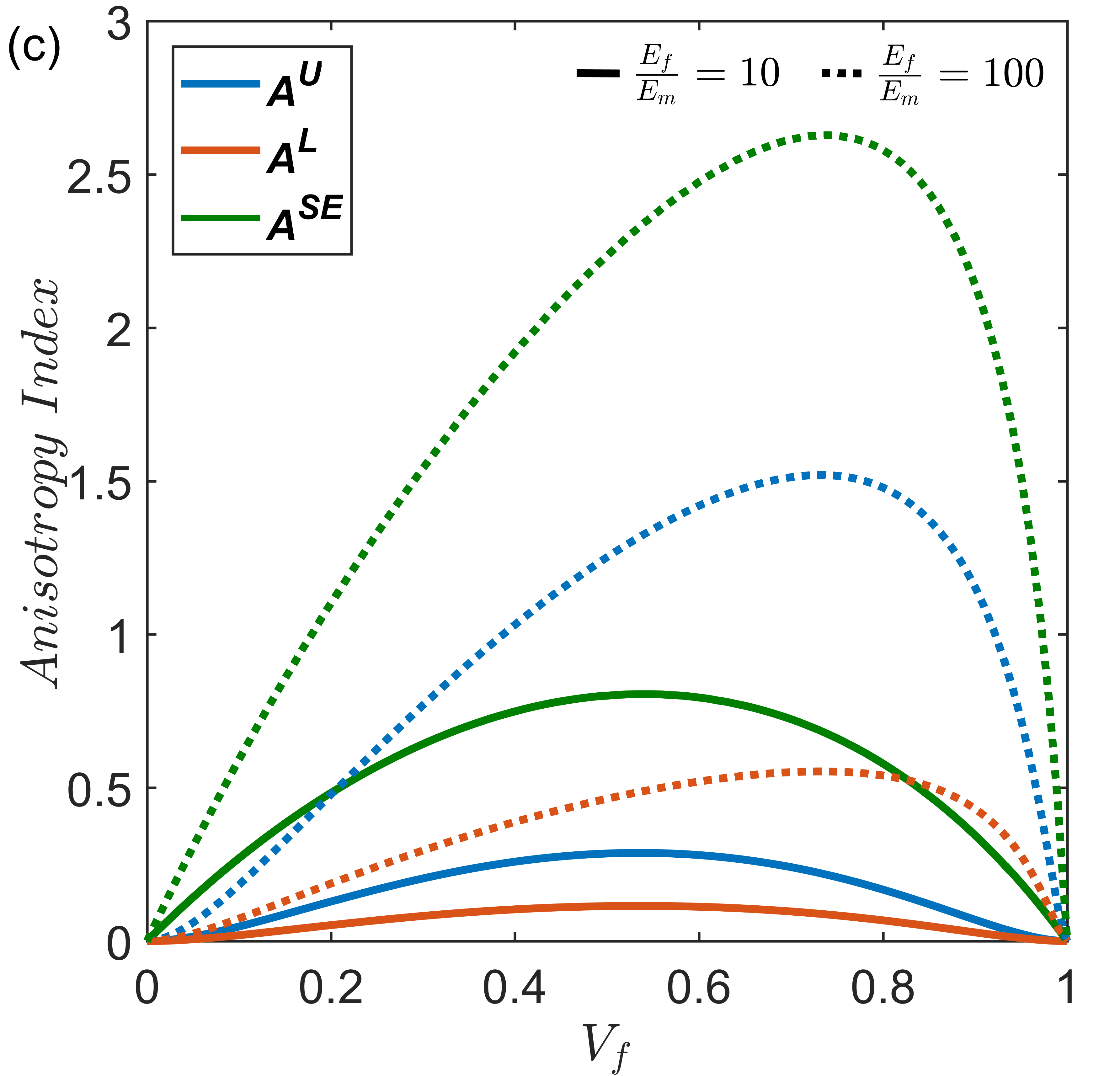
Figure 2: Influence of microstructural and material descriptors on anisotropy in two phase particulate reinforced composite materials: effect of (a) overall shape of the particulates and particulate volume fraction ($E_{f}/E_{m}=10$) and (b) aspect ratio of prolate ellipsoids highlighting the influence of microstructural descriptors ($E_{f}/E_{m}=10$), and (c) elastic contrast ratio highlighting the influence of material descriptors (prolate ellipsoids, $\alpha=5$).

IV Discussion

The reinterpretation of anisotropy indices in the context of heterogeneous materials can demonstrated by considering composite materials due to the availability of closed form expressions for idealized reinforcement shapes. Considering a two phase composite material consisting of aligned isotropic ellipsoidal particulates embedded in isotropic matrix, the effective elastic stiffness tensor accounting for the elastic properties and volume fractions of the constituent phases along with the shape of the particulates is given by Mori-Tanaka approach [34] in the following form.

$$C^{*}=(1-V_{f})C^{m}A^{MT}+V_{f}C^{f}A^{MT}A^{Eshelby}$$ (15)

Where $V_{f}$ is the volume fraction of the particulate phase, $C^{f}$ is the stiffness tensor of the particulate phase, $C^{m}$ is the stiffness tensor of the matrix phase and $A^{MT}$ is the Mori-Tanaka strain concentration tensor given by

$$A^{MT}=[(1-V_{f})I+V_{f}A^{Eshelby}]^{-1}$$ (16)

Where $I$ is identity matrix and $A^{Eshelby}$ is the Eshelby strain concentration tensor in terms of the Eshelby tensor $S$ [35] that accounts for the particulate shape.

$$A^{Eshelby}=[I+SC^{m}(C^{f}-C^{m})]^{-1}$$ (17)

The advantage of Mori-Tanaka approach is the ability to consider shape parameters of general ellipsoidal shapes along with volume fractions and constituent phase properties in effective property estimation. With the determination of $C^{*}$, the influence of constituent properties, relative content, particulate shape and aspect ratio on the anisotropy of two phase composite materials can be evaluated.

The microstructural features that influence $C^{*}$ and consequently the extent of anisotropy are the reinforcement volume fraction, reinforcement shape and aspect ratio of a particular shape under consideration. Assuming that the reinforcement and matrix are individually isotropic with elastic contrast ratio $E_{f}/E_{m}=10$, the role of volume fractions and overall shape of the particulates in influencing anisotropy can be inferred from the variation of anisotropy indices with particulate volume fractions as shown in Fig. 2. The anisotropy indices increase from zero, reach a peak and reduce back to zero indicating that the presence of a secondary phase with elastic property mismatch causes a deviation from isotropy even though the constituents are individually isotropic.

The nature of variation of anisotropy indices differ across prolate and oblate ellipsoidal particulates (Fig. 2) highlighting the effect of overall shape of secondary phase on the extent of anisotropy. Further, anisotropy increases with increasing aspect ratio ($\alpha$) across the range of volume fractions in the case of prolate ellipsoids (Fig. 2) highlighting the effect of shape parameters on anisotropy. The overall shape and the shape parameters along with the particulate volume fractions can be collectively termed as the microstructural descriptors that influence anisotropy in heterogeneous materials.

Elastic contrast, defined as the ratio of the Young’s moduli of the constituent phases ($E_{f}/E_{m}$), is a crucial material descriptor in heterogeneous materials. Considering prolate ellipsoidal particulates, elastic contrast has a significant influence on the extent of anisotropy across the range of volume fractions as seen in Fig. 2. Variation in elastic contrast not only changes the extent of anisotropy across the range of volume fractions but also influences the peak anisotropy and the particulate volume fraction at which the peak anisotropy occurs. The significant influence of elastic contrast in controlling the extent of anisotropy makes it a key material descriptor influencing anisotropy in heterogeneous materials in addition to microstructural descriptors discussed previously.

In the backdrop of anisotropy arising from heterogeneity, the conditions that lead to overall isotropy in heterogeneous material systems is of special interest. Overall isotropy can be inferred by anisotropy indices $A^{U}$, $A^{L}$ and $A^{SE}$ being consistently zero with a variation in material and microstructral descriptors. Two phase particle reinforced composite materials exhibit overall isotropy indicated by anisotropy indices going to zero when the particulates are spherical (Fig.3) and when the contrast ratio is unity i.e. $E_{f}/E_{m}=1$ (Fig.3). Spheres have identical response in all directions leading to overall isotropy in heterogeneous materials with spherical particulates. Contrast ratio being unity signifies identical properties of the constituent phases that is analogous to homogeneous material.

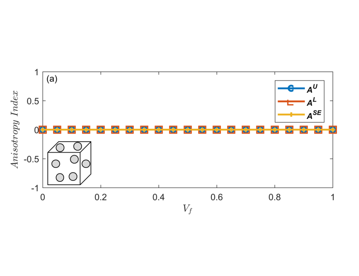
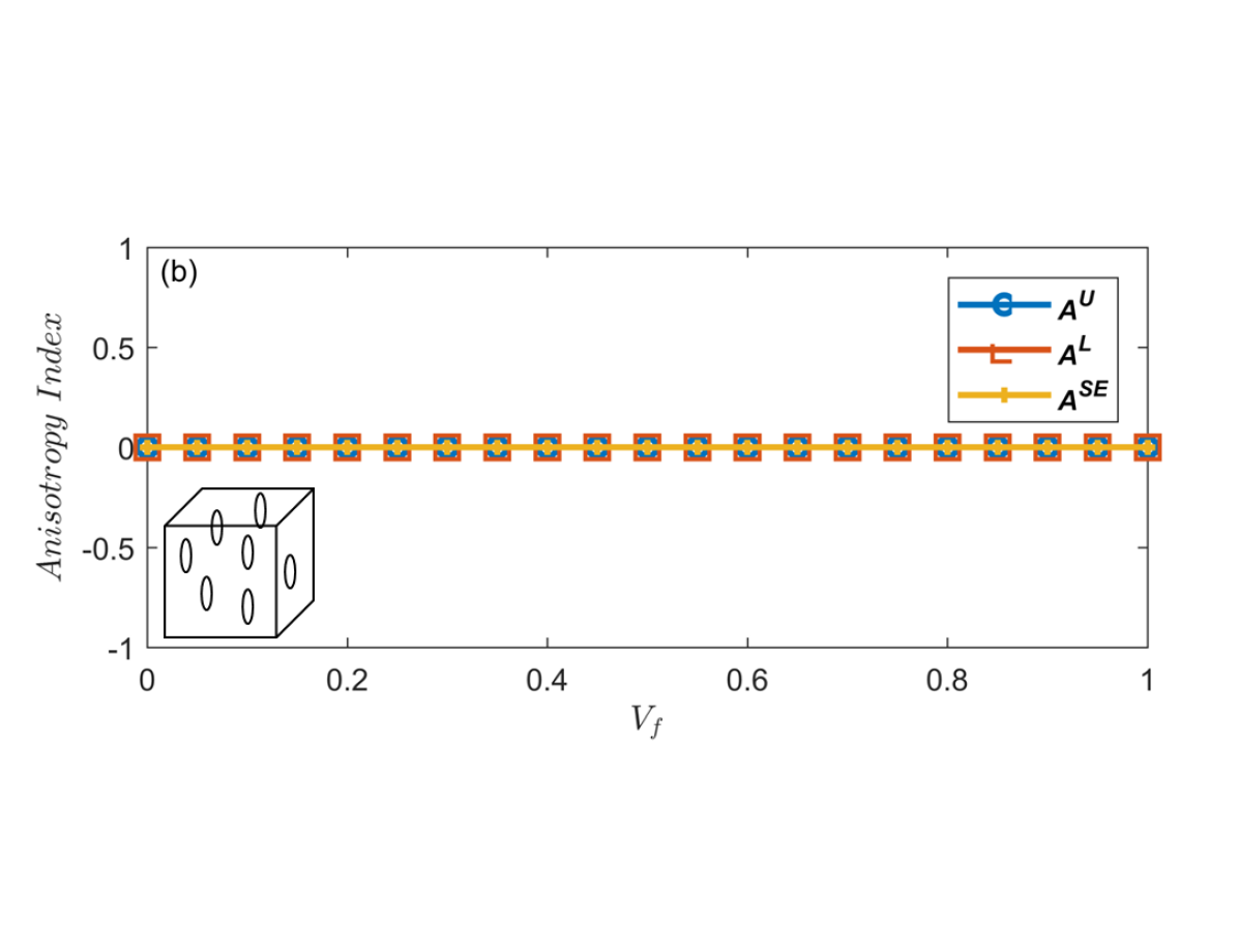
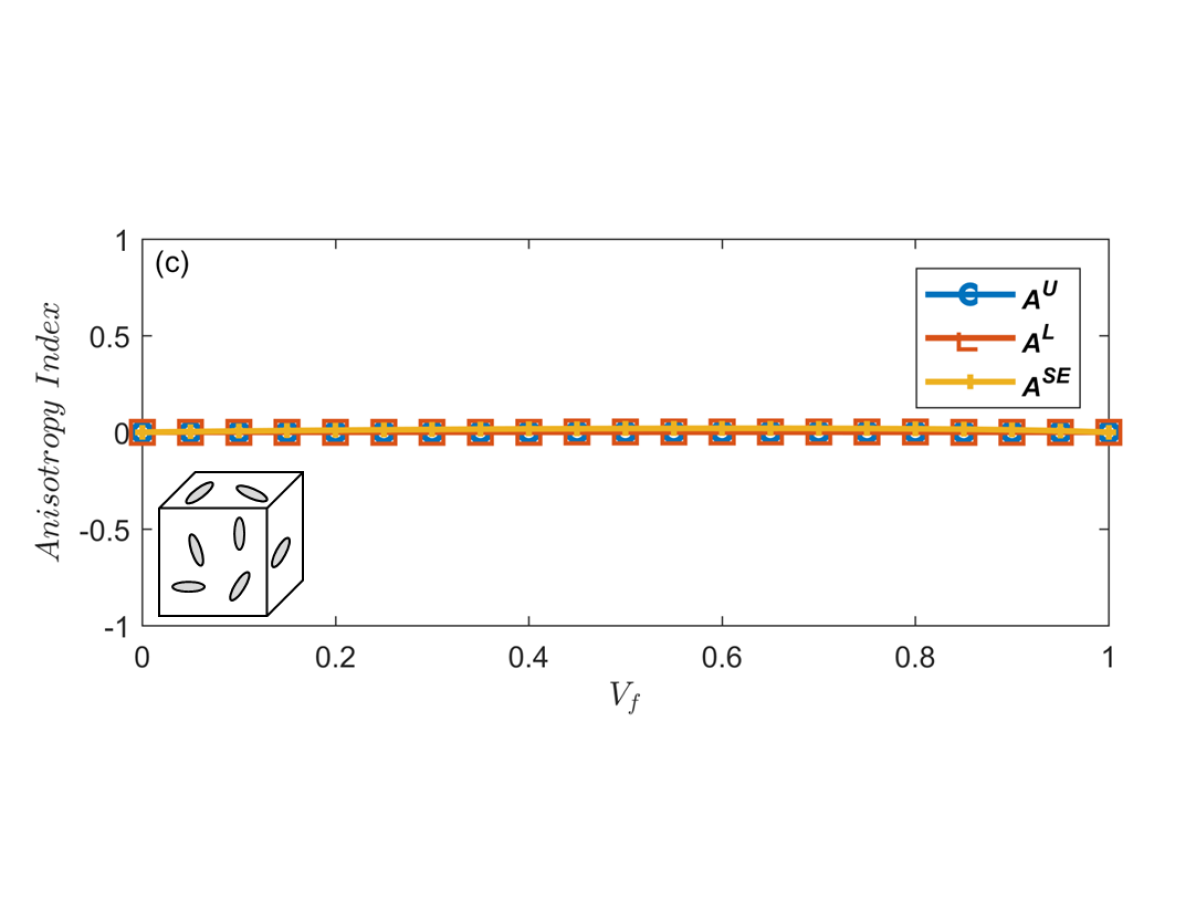
Figure 3: Two phase composite materials consisting of isotropic ellipsoidal particulates in isotropic matrix lead to overall isotropy indicated by anisotropy indices $A^{U}$,$A^{L}$,$A^{SE}$ being zero under the following conditions (composite configuration mentioned in brackets): (a) particulates are spherical ($E_{f}/E_{m}=10$), (b) aligned particulates of general ellipsoidal shapes have a contrast ratio of 1 (aligned prolate ellipsoids, $\alpha=5$, $E_{f}/E_{m}=1$), (c) randomly oriented prolate ellipsoids ($\alpha=5$, $E_{f}/E_{m}=10$), and (d) randomly oriented oblate ellipsoids ($\alpha=1/5$, $E_{f}/E_{m}=10$).

While isotropic matrices consisting of randomly oriented reinforcement phases of ellipsoidal shapes are stated to exhibit overall isotropy, the present approach enables a rigorous proof of the same. Consider a two phase particle reinforced composite material with randomly oriented isotropic ellipsoidal particles embedded in isotropic matrix. Random distribution of the reinforcing phases can be modeled by co-ordinate transformation of the strain concentration tensor and averaging the transformed strain concentration tensor over all possible orientations. Strain concentration tensor follows the transformation rule for fourth order tensors i.e. $\bar{A}^{Eshelby}=Q_{ip}Q_{jp}Q_{kr}Q_{ls}A^{Eshelby}$ with $Q_{ij}$ representing the rotation tensor and considering the orientation averaged quantity denoted by $\left\langle{}\right\rangle$ in the following form [ferrari1989effective].

$$\left\langle{A^{Eshelby}}\right\rangle=\dfrac{\int_{-\pi}^{\pi}\int_{0}^{\pi}\int_{0}^{\pi/2}[\bar{A}^{Eshelby}(\phi,\gamma,\psi)\ sin\gamma\ d\phi\ d\gamma\ d\psi]}{\int_{-\pi}^{\pi}\int_{0}^{\pi}\int_{0}^{\pi/2}sin\gamma\ d\phi\ d\gamma\ d\psi}$$ (18)

Where $\gamma,\phi,\psi$ represent orientations w.r.t global co-ordinates. The Mori-Tanaka strain concentration tensor for random orientation of particulate phases is given by the following expression.

$$A^{MT}_{Random}=[(1-V_{f})I+V_{f}\left\langle{A^{Eshelby}}\right\rangle]^{-1}$$ (19)

The effective elastic properties with randomly oriented particulate phase ($C^{*}_{Random}$) can be evaluated considering the orientation averaged strain concentration tensor in the following form.

$$C^{*}_{Random}=(1-V_{f})C^{m}A^{MT}_{Random}+V_{f}C^{f}A^{MT}_{Random}\left\langle A^{Eshelby}\right\rangle$$ (20)

Evaluation of $A^{U}$, $A^{L}$ and $A^{SE}$ considering $C^{*}_{Random}$ corresponding to randomly oriented ellipsoidal particulates reveal that they are zero across the range of volume fractions (Figs.3,3) indicating overall isotropy irrespective of overall shape, shape parameters and contrast ratio. Previous observations regarding overall isotropy in 2 phase composites with randomly oriented ellipsoidal particles (Benveniste[34] and references therein) can be rigorously proved with the present approach. However, such observations regarding overall isotropy cannot be extended directly to the case where the constituents themselves are anisotropic.

Homogeneous elastic medium containing dry pores (voids) and cracks can be considered as a special case of heterogeneous materials with the pores/cracks representing a distinct phase with zero elastic stiffness [36, 37]. The effective elastic stiffness tensor of a material consisting of ellipsoidal pores $C^{*}_{Pore}$ accounting for the pore volume fraction $V_{P}$ and shape of pores is given in the following form.

$$C^{*}_{Pore}=(1-V_{P})C^{m}A^{MT}$$ (21)

Where $C^{m}$ is the stiffness tensor of the matrix phase. Mori-Tanaka strain concentration tensor $A^{MT}$ and Eshelby strain concentration $A^{Eshelby}$ are obtained by replacing $V_{f}$ with $V_{P}$ and $C^{m}$ by a null matrix in Eq. 16 and Eq. 17 respectively. Evaluation of anisotropy indices with $C^{*}_{Pore}$ following the approach for anisotropy quantification in two phase composite materials provides an insight into the anisotropy caused by the presence of porosity in homogeneous materials.

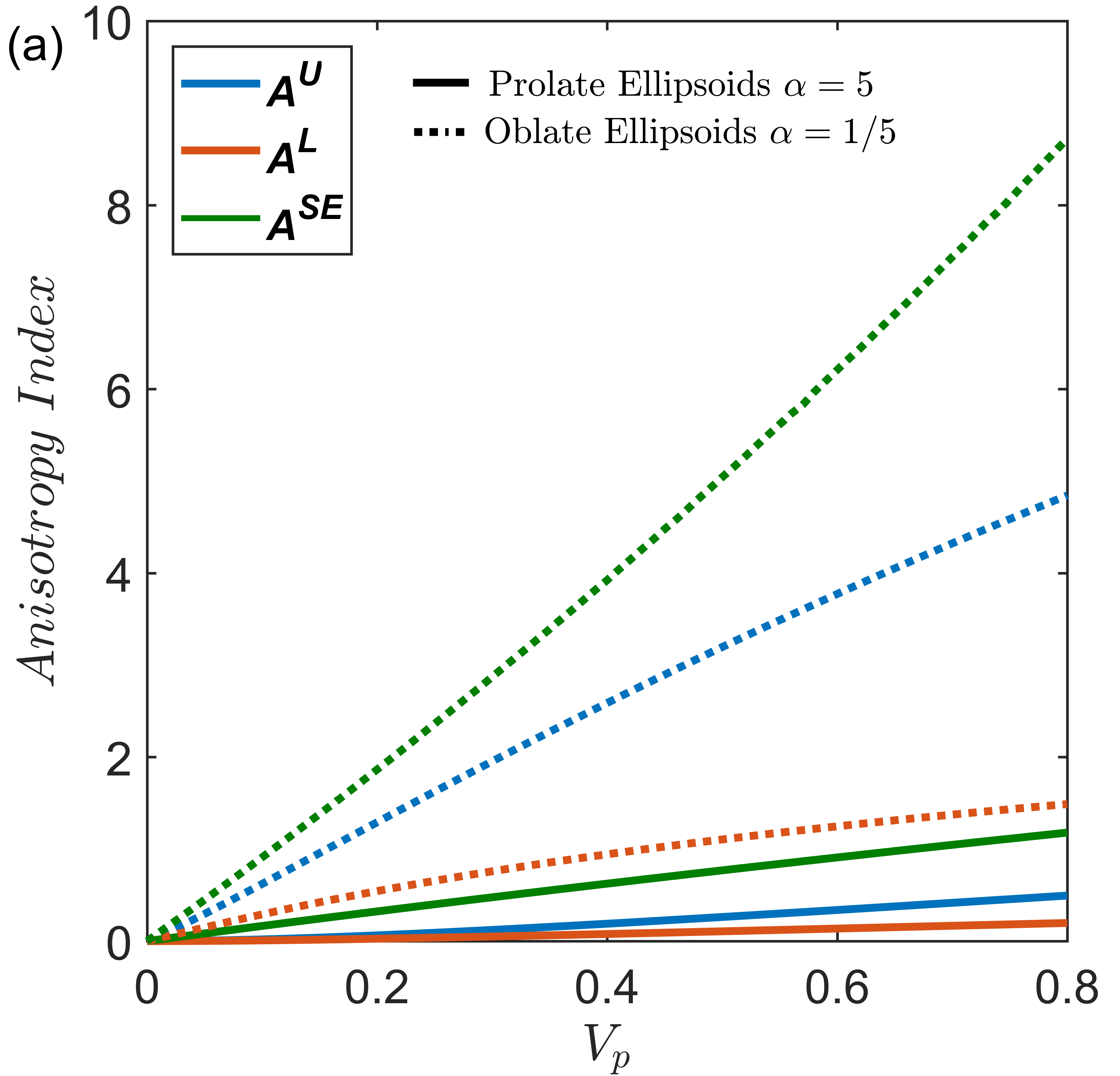
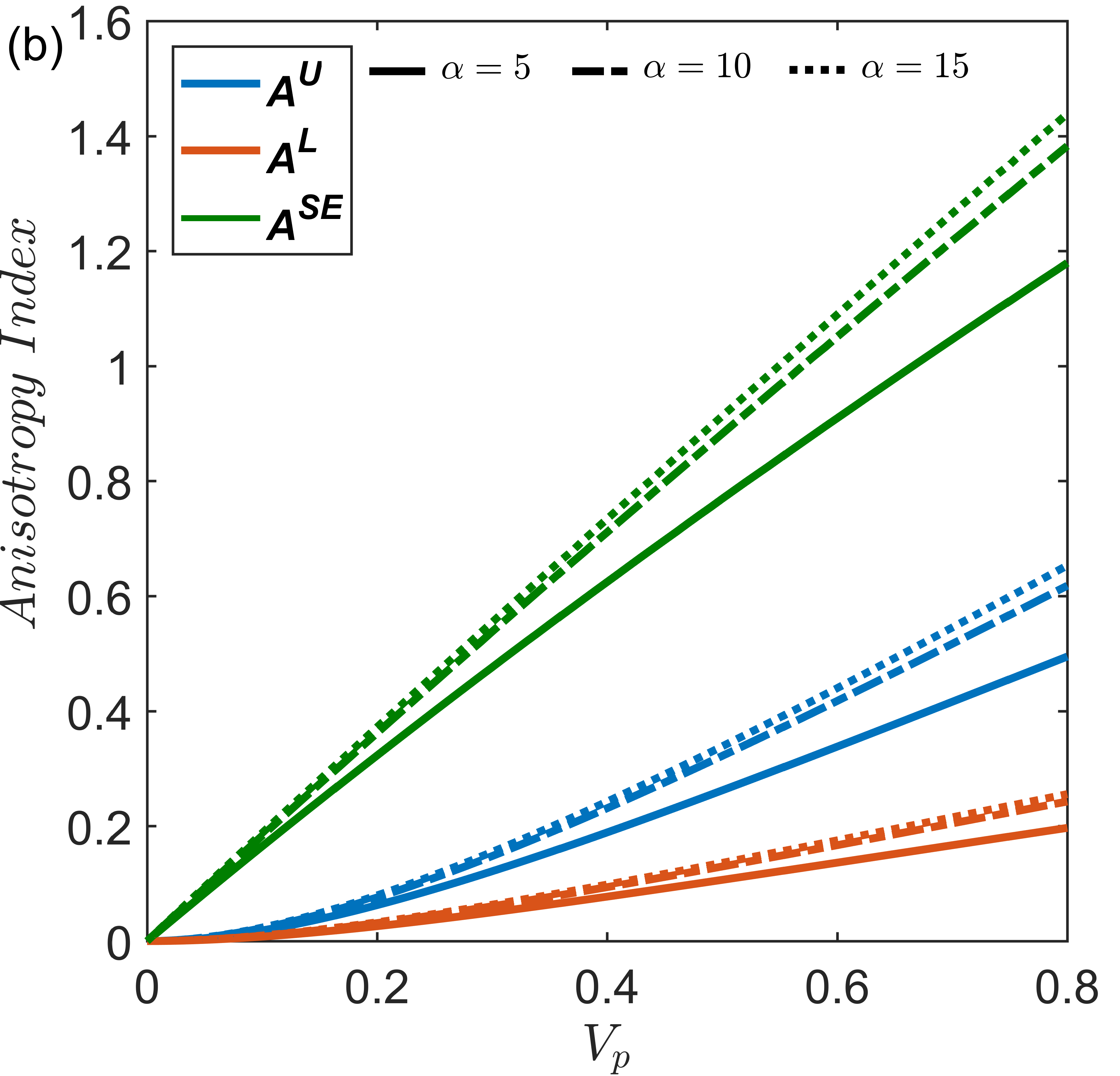
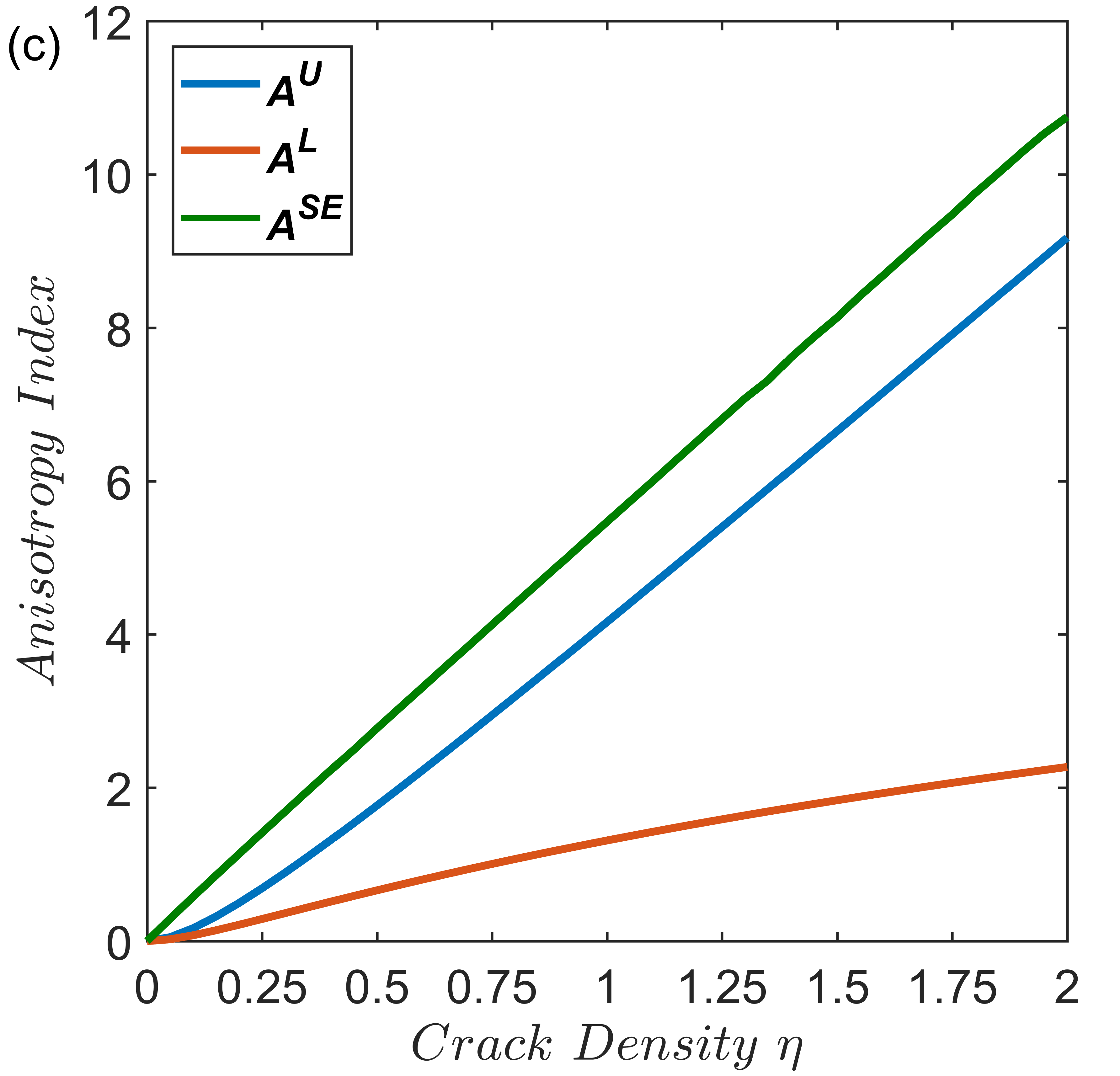
Figure 4: Influence of aligned pores and cracks on anisotropy in homogeneous materials: (a) variation of anisotropy with pore volume fraction $V_{p}$ highlighting the effect of overall shape of ellipsoidal pores on anisotropy, and (b) effect of aspect ratio of prolate ellipsoidal pores emphasizing the influence of shape parameters and (c) influence of circular cracks.

Aligned ellipsoidal pores in an isotropic homogeneous material leads to anisotropy with the extent of anisotropy varying with pore volume fraction $V_{P}$ as shown in Fig. 4. Anisotropy in porous materials vary monotonically with pore volume fraction ($V_{P}$) in stark contrast to two phase heterogeneous materials. Pore shape has a significant effect on the nature of anisotropy variation with prolate and oblate ellipsoidal pores exhibiting markedly different trends as shown in Fig. 4. While increasing pore aspect ratio leads to increase in anisotropy as shown in Fig. 4, the influence of aspect ratio on anisotropy is to a lower extent compared to the overall shape of porosity. Thus, the pore volume fraction, pore shape and aspect ratio form the microstructural descriptors that influence anisotropy in porous materials. Analogously to two phase composite materials, homogeneous materials consisting of spherical pores or randomly oriented ellipsoidal pores exhibit overall isotropy.

Circular cracks represent the extreme case of collapsed discus shaped pores with the aspect ratio tending to zero ($\alpha\rightarrow 0$). Consequently, the volume of individual cracks tend to zero. Quantifying crack content by crack density ‘$\eta$’ that is related to the crack volume fraction $V_{C}$ as $\eta=3V_{C}/4\pi\alpha$, it can be seen that aligned circular cracks lead to a substantial deviation from isotropy even at low concentrations as shown in Fig. 4. Large deviation from isotropy even at low crack concentrations indicate that cracks have a much more significant effect on deviation isotropy than pores.

While $A^{U}$, $A^{L}$ and $A^{SE}$ can be utilized to quantify anisotropy in heterogeneous materials, the most suitable index for anisotropy quantification is a pertinent question. $A^{U}$ and $A^{L}$ have simple closed form expressions in terms of the effective stiffness and compliance matrices of a heterogeneous material leading to ease of evaluation but their physical meaning is difficult to comprehend. $A^{SE}$ on the other hand requires optimization which is computationally expensive and sensitive to the optimization parameters. However, $A^{SE}$ has a clear physical meaning and has an advantage over $A^{U}$ and $A^{L}$ in the form of easy generalization to consider physical fields other than mechanical loading, multiphysics phenomenon and non-linearity. These factors can drive the selection of the appropriate anisotropy index.

The proposed approach to quantify anisotropy in heterogeneous materials along with the presented results open up the exploration of the role microstructural features such as multi-phase reinforcements, presence of pores/cracks along with secondary phases and microstructure statistics (reinforcement/pore aspect ratio and orientation distribution) in influencing anisotropy. In random heterogeneous materials, salient microstructural features such as phase topology and connectivity also play a role in influencing anisotropy and the current approach for anisotropy quantification can form the basis for anisotropy tuning in composite [38] and architectured materials [39, 40].

V Conclusion

In conclusion, a novel approach for anisotropy quantification in heterogeneous materials has been presented in the present paper by reinterpreting anisotropy indices proposed in the context of single crystals considering the effective elastic properties of heterogeneous materials. The reinterpreted anisotropy indices are applicable to any class of heterogeneous materials utilizing appropriate homogenization techniques. Anisotropy quantification in two-phase composite materials reveals that heterogeneity with elastic mismatch between the constituent phases leads to anisotropy. The influence of material and microstructural descriptors on anisotropy in heterogeneous materials is a significant distinction from single crystals. Specific cases leading to overall isotropy in two phase composite materials and extension of the approach to consider porosity and cracks have also been presented demonstrating the applicability of the approach to any class of heterogeneous materials. The approach to quantify anisotropy in heterogeneous materials open up the exploration of salient microstructral features and microstructural statistics in influencing anisotropy in heterogeneous, porous and architectured materials. Additionally, the proposed approach can be extended to consider other physical fields, multiphysics phenomena and non-linearity in heterogeneous materials.

References

- Ingel and III [1988] R. P. Ingel and D. L. III, J. Am. Cer. Soc. 71, 265 (1988).
- Brenner et al. [2009] R. Brenner, R. Lebensohn, and O. Castelnau, Int. J. Sol. Struct. 46, 3018 (2009).
- Hashin [1983] Z. Hashin, J. App. Mech. 50, 481 (1983).
- Katz [1980] J. L. Katz, Nature 283, 106 (1980).
- Katz and Meunier [1987] J. L. Katz and A. Meunier, J. Biomech. 20, 1063 (1987).
- Sondergeld and Rai [2011] C. H. Sondergeld and C. S. Rai, The Leading Edge 30, 324 (2011).
- Li et al. [2020] R. Li, Q. Shao, E. Gao, and Z. Liu, Ext. Mech. Lett. 34, 100615 (2020).
- Schmitz et al. [1989] A. Schmitz, M. Chandrasekaran, G. Ghosh, and L. Delaey, Acta Metall. 37, 3151 (1989).
- Fichant et al. [1997] S. Fichant, G. Pijaudier-Cabot, and C. La Borderie, Mech. Res. Comm. 24, 109 (1997).
- Han et al. [2003] X. Han, N. M. Ghoniem, and Z. Wang, Phil. Mag. 83, 3705 (2003).
- Brugués et al. [2008] J. Brugués, J. Ignés-Mullol, J. Casademunt, and F. Sagués, Phys. Rev. Lett. 100, 037801 (2008).
- Tvergaard and Hutchinson [1988] V. Tvergaard and J. W. Hutchinson, J. Am. Cer. Soc. 71, 157 (1988).
- Li et al. [2002] J. Li, K. J. Van Vliet, T. Zhu, S. Yip, and S. Suresh, Nature 418, 307 (2002).
- Böhlke and Brüggemann [2001] T. Böhlke and C. Brüggemann, Tech. Mech. 21, 145 (2001).
- Nordmann et al. [2018] J. Nordmann, M. Aßmus, and H. Altenbach, Cont. Mech. Therm. 30, 689 (2018).
- Coleman and Noll [1964] B. D. Coleman and W. Noll, Arch. Rat. Mech. Ana. 15, 87 (1964).
- Zener [1948] C. Zener, Elasticity and Anelasticity of Metals (University of Chicago Press, 1948).
- Chung and Buessem [1967] D. Chung and W. Buessem, J. Appl. Phys. 38, 2010 (1967).
- Ledbetter and Migliori [2006] H. Ledbetter and A. Migliori, J. Appl. Phys. 100, 063516 (2006).
- Ranganathan and Ostoja-Starzewski [2008] S. I. Ranganathan and M. Ostoja-Starzewski, Phys. Rev. Lett. 101, 055504 (2008).
- Nye [1985] J. F. Nye, Physical properties of crystals: their representation by tensors and matrices (Oxford university press, 1985).
- Wang and Zheng [2007] L.-F. Wang and Q.-S. Zheng, Appl. Phys. Lett. 90, 153113 (2007).
- Rychlewski and Zhang [1989] J. Rychlewski and J. Zhang, Arch. Mech 47, 697 (1989).
- Rychlewski [1984] J. Rychlewski, Czech. J. Phys. B 34, 499 (1984).
- Fang et al. [2019] Y. Fang, Y. Wang, H. Imtiaz, B. Liu, and H. Gao, Phys. Rev. Lett. 122, 045502 (2019).
- Kube [2016] C. M. Kube, AIP Adv. 6, 095209 (2016).
- Hill [1952] R. Hill, Proc. Phys. Soc. A 65, 349 (1952).
- Hill [1963] R. Hill, J. Mech. Phys. Sol. 11, 357 (1963).
- Nemat-Nasser and Hori [1993] S. Nemat-Nasser and M. Hori, Micromechanics: Overall properties of heterogeneous materials (Elsevier, 1993).
- Kube and De Jong [2016] C. M. Kube and M. De Jong, J. Appl. Phys. 120, 165105 (2016).
- Wei et al. [2021] A. Wei, J. Xiong, W. Yang, and F. Guo, Ext. Mech. Lett. 43, 101173 (2021).
- Mehrabadi et al. [1995] M. M. Mehrabadi, S. C. Cowin, and J. Jaric, Int. J. Sol. Struct. 32, 439 (1995).
- Norris [2008] A. N. Norris, Mat. Mech. Sol. 13, 465 (2008).
- Benveniste [1987] Y. Benveniste, Mech. Mater 6, 147 (1987).
- Eshelby [1957] J. D. Eshelby, Proc. R. Soc. A 241, 376 (1957).
- Zhao et al. [1989] Y. Zhao, G. Tandon, and G. Weng, Acta. Mech. 76, 105 (1989).
- Pan and Weng [1995] H. Pan and G. Weng, Acta Mech. 110, 73 (1995).
- Vidyasagar et al. [2018] A. Vidyasagar, S. Krödel, and D. M. Kochmann, Proc. R. Soc. A 474, 20180535 (2018).
- Kumar et al. [2020] S. Kumar, S. Tan, L. Zheng, and D. M. Kochmann, Comp. Mat. 6, 1 (2020).
- Zheng et al. [2021] L. Zheng, S. Kumar, and D. M. Kochmann, Comp. Meth. App. Mech. Eng. 383, 113894 (2021).