Renormalization for a model of photon scattering
off a charged harmonic oscillator

Abstract

In the electric dipole approximation the model of a charged harmonic oscillator interacting with the radiation field becomes quadratic and soluble, but it needs a UV cutoff for the photon frequency. The model’s renormalizability is only apparent; physics requires that the cutoff be kept finite. The cutoff plays the role of a parameter that characterizes the high frequency behavior of the photon cross section.

I Brief introduction

Exponential decays of excited states were first derived from quantum mechanics by Weisskopf and Wigner Weisskopf and Wigner (1930a, b). Their derivation makes it clear that the decay has nothing to do with the non-linearity of the system, but it is due to the mixing of discrete excited states with a continuum of states involving photons. This type of mixing has been known as configuration interactions in the literature.

U. Fano was the first to diagonalize a generic hamiltonian with a configuration interaction Fano (1961). The solution is based on the method that Dirac used for the derivation of resonance scattering Dirac ; Dirac (1982). Fano applied the result, known as Fano’s profile, to the inelastic electron scattering by He near the resonance corresponding to a double excitation to $2s2p$.

Fano’s model has been studied as a simple model of renormalization in Sonoda (2014). (Due to the author’s ignorance, Sonoda (2014) has no reference to Fano’s earlier works.) The present paper is an extension, and differs technically from Sonoda (2014) in two aspects. First, the model is constructed in the lagrangian formalism as opposed to the hamiltonian formalism. Second, the time-ordered propagator of the oscillator coordinate is considered as opposed to the retarded Green function of the hamiltonian. Otherwise, the same technique based on the analyticity of the Green function is used.

The purpose of the paper is to gain further insights into the physics of renormalization. The outline of the paper is as follows. In Sec. II we introduce the model of photon scattering off a charged harmonic oscillator. We study the field theoretic properties of the model as it is without questioning the validity of the electric dipole approximation. In Sec. III we introduce a sharp cutoff $\omega_{H}$ for the photon’s frequency. Two renormalized parameters are defined: $\Omega_{r}$ and $r_{0,r}$. We show that $\omega_{H}$ has a maximum; hence, we cannot take the limit $\omega_{H}\to+\infty$. In Sec. IV we first sketch the derivation of the photon scattering cross section $\sigma(\omega)$ in terms of the spectral function of the propagator. We then show how $\omega_{H}$ determines the behavior of $\sigma(\omega)$ for $\Omega_{r}\ll\omega\ll\omega_{H}$. In Sec. V we discuss the naive continuum limit $\omega_{H}\to+\infty$. We explain that the propagator obtains a tachyon with a negative probability. In Sec. VI we explain that $\sigma(\omega)$ does not depend on the details of the cutoff. We show how to define $\omega_{H}$ for a smooth cutoff. We conclude the paper in Sec. VII. In Appendix we explain that the tachyon in the naive continuum limit is a consequence of the negative kinetic term in the lagrangian.

II The model

We consider the lagrangian of a charged harmonic oscillator interacting with the radiation field given by

$$L=\frac{m}{2}\frac{d}{dt}\vec{x}\cdot\frac{d}{dt}\vec{x}-\frac{m\Omega^{2}}{2}\vec{x}\,^{2}+e\frac{d}{dt}\vec{x}\cdot\vec{A}(t,\vec{x})+\int d^{3}x\,\frac{1}{2}\left(\partial_{t}\vec{A}\cdot\partial_{t}\vec{A}+\vec{A}\cdot\nabla^{2}\vec{A}\right)\,,$$ (1)

where the vector potential satisfies the Coulomb gauge condition

$$\nabla\cdot\vec{A}=0\,.$$ (2)

The lagrangian becomes quadratic and thus soluble in the electric dipole approximation:

$$L=\frac{m}{2}\frac{d}{dt}\vec{x}\cdot\frac{d}{dt}\vec{x}-\frac{m\Omega^{2}}{2}\vec{x}\,^{2}+e\frac{d}{dt}\vec{x}\cdot\vec{A}(t,\vec{0})+\int d^{3}x\,\frac{1}{2}\left(\partial_{t}\vec{A}\cdot\partial_{t}\vec{A}+\vec{A}\cdot\nabla^{2}\vec{A}\right)\,,$$ (3)

where the dependence of the vector potential on $\vec{x}$ is ignored in the interaction term. The approximation is valid as long as the wave length of a photon is long compared with the size of the oscillator:

$$\lambda=\frac{2\pi}{\omega}>\frac{1}{\sqrt{m\Omega}}\,.$$ (4)

In the following we examine the field theoretic properties of the model given by (3), where even the photons violating (4) are included. We are especially interested in the question of renormalizability.

We expand

$$\vec{A}(t,\vec{x})=\frac{1}{\sqrt{V}}\sum_{\vec{k}}\sum_{\vec{\epsilon}}\vec{\epsilon}\,\varphi_{\vec{k},\vec{\epsilon}}\,(t)e^{i\vec{k}\cdot\vec{x}}\,,$$ (5)

where $V$ is the space volume, $\vec{\epsilon}$ is a unit polarization vector orthogonal to $\vec{k}$, and $\varphi_{\vec{k},\vec{\epsilon}}$ satisfies $\varphi_{-\vec{k},\vec{\epsilon}}=\varphi_{\vec{k},\vec{\epsilon}}^{*}$ . We then obtain

$$\int d^{3}x\,\frac{1}{2}\left(\partial_{t}\vec{A}\cdot\partial_{t}\vec{A}+\vec{A}\cdot\nabla^{2}\vec{A}\right)=\sum_{\vec{k}}\sum_{\vec{\epsilon}}\frac{1}{2}\left(\partial_{t}\varphi_{-\vec{k},\vec{\epsilon}}\,\partial_{t}\varphi_{\vec{k},\vec{\epsilon}}-k^{2}\varphi_{-\vec{k},\vec{\epsilon}}\,\varphi_{\vec{k},\vec{\epsilon}}\right)\,.$$ (6)

Defining two real fields

$$\phi_{n}\equiv\frac{1}{\sqrt{2}}\left(\varphi_{\vec{k},\vec{\epsilon}}+\varphi_{-\vec{k},\vec{\epsilon}}\right),\quad\psi_{n}\equiv\frac{1}{\sqrt{2}}\frac{1}{i}\left(\varphi_{\vec{k},\vec{\epsilon}}-\varphi_{-\vec{k},\vec{\epsilon}}\right)\,,$$ (7)

for $n=(\vec{k},\vec{\epsilon})$, we obtain

$$\int d^{3}x\,\frac{1}{2}\left(\partial_{t}\vec{A}\cdot\partial_{t}\vec{A}+\vec{A}\cdot\nabla^{2}\vec{A}\right)=\sum_{n}\frac{1}{2}\left((\partial_{t}\phi_{n})^{2}-\omega_{n}^{2}\phi_{n}^{2}\right)+\sum_{n}\frac{1}{2}\left((\partial_{t}\psi_{n})^{2}-\omega_{n}^{2}\psi_{n}^{2}\right)\,,$$ (8)

where $\omega_{n}=k\equiv|\vec{k}|$, and the sum is over a half of the $\vec{k}$ space and $\vec{\epsilon}$. (If $\vec{k}$ is included in the sum, then $-\vec{k}$ is not.) We will drop $\psi$’s with even parity from now on, since only $\phi$’s with odd parity interact with the charged oscillator. Denoting $\vec{X}=\sqrt{m}\,\vec{x}$, we obtain

$$L=\frac{1}{2}\frac{d}{dt}\vec{X}\cdot\frac{d}{dt}\vec{X}-\Omega^{2}\frac{1}{2}\vec{X}\,^{2}+\sum_{n}\frac{1}{2}\left((\partial_{t}\phi_{n})^{2}-\omega_{n}^{2}\phi_{n}^{2}\right)+\frac{e}{\sqrt{m}}\frac{d}{dt}\vec{X}(t)\cdot\sqrt{\frac{2}{V}}\sum_{n}\vec{\epsilon}_{n}\phi_{n}(t)\,.$$ (9)

This is the model we are going to solve.

In the frequency space the free propagators are given by

$$\left\langle X_{i}(\omega)X_{j}(-\omega)\right\rangle_{0} =\delta_{ij}\frac{i}{\omega^{2}-\Omega^{2}+i\epsilon}\,,$$ (10a)

$$\left\langle\phi_{n}(\omega)\phi_{n}(-\omega)\right\rangle_{0} =\frac{i}{\omega^{2}-\omega_{n}^{2}+i\epsilon}\,,$$ (10b)

where the product is time ordered. Hence, to the second order in perturbation, the propagator of $\vec{X}$ is obtained as

$$\left\langle X_{i}(\omega)X_{j}(-\omega)\right\rangle$$

$$\simeq\frac{i}{\omega^{2}-\Omega^{2}+i\epsilon}\left(\delta_{ij}-\frac{2e^{2}}{mV}\omega^{2}\sum_{n}\epsilon_{n,i}\epsilon_{n,j}\frac{i}{\omega^{2}-\omega_{n}^{2}+i\epsilon}\frac{i}{\omega^{2}-\Omega^{2}+i\epsilon}\right)\,.$$ (11)

Summing over two polarization vectors, we obtain

$$\sum_{\vec{\epsilon}}\epsilon_{i}\epsilon_{j}=\delta_{ij}-\frac{k_{i}k_{j}}{k^{2}}\,.$$ (12)

Averaging over the directions of $\vec{k}$, we can replace this by

$$\sum_{\vec{\epsilon}}\epsilon_{i}\epsilon_{j}=\frac{2}{3}\delta_{ij}\,.$$ (13)

Hence, we obtain

$$\sum_{n}\epsilon_{n,i}\epsilon_{n,j}\frac{1}{\omega^{2}-\omega_{n}^{2}+i\epsilon}=\frac{2}{3}\delta_{ij}\frac{1}{2}\sum_{\vec{k}}\frac{1}{\omega^{2}-k^{2}+i\epsilon}\,,$$ (14)

where the factor $\frac{1}{2}$ is necessary since the sum over $n$ includes only a half of the $\vec{k}$ space. We then obtain

$$\left\langle X_{i}(\omega)X_{j}(-\omega)\right\rangle$$

$$\simeq\delta_{ij}\frac{i}{\omega^{2}-\Omega^{2}+i\epsilon}\left(1+\frac{2e^{2}}{3mV}\omega^{2}\sum_{\vec{k}}\frac{1}{\omega^{2}-k^{2}+i\epsilon}\frac{1}{\omega^{2}-\Omega^{2}+i\epsilon}\right)\,.$$ (15)

It is straightforward to go beyond the second order perturbation. Summing the corresponding geometric series, we obtain the exact full propagator as

$$\delta_{ij}\,G(\omega^{2}+i\epsilon)\equiv\frac{1}{i}\left\langle X_{i}(\omega)X_{j}(-\omega)\right\rangle=\delta_{ij}\frac{1}{\omega^{2}-\Omega^{2}-\frac{2e^{2}}{3mV}\omega^{2}\sum_{\vec{k}}\frac{1}{\omega^{2}-k^{2}+i\epsilon}}\,.$$ (16)

We now compute

$$\frac{2e^{2}}{3mV}\sum_{\vec{k}}\delta(k-\omega) =\frac{2e^{2}}{3mV}V\int\frac{d^{3}k}{(2\pi)^{3}}\delta(k-\omega)$$

$$=\frac{2e^{2}}{3m}\frac{4\pi}{(2\pi)^{3}}\omega^{2}=\frac{4}{3\pi}r_{0}\omega^{2}\,,$$ (17)

where

$$r_{0}\equiv\frac{e^{2}}{4\pi}\frac{1}{m}$$ (18)

would be the classical electron radius if $m$ were the electron mass, and $e$ the elementary charge. We can write the inverse propagator as

$$\frac{1}{G(\omega^{2}+i\epsilon)}=\omega^{2}-\Omega^{2}-\omega^{2}\frac{4}{3\pi}r_{0}\int_{0}^{\infty}d\omega^{\prime}\,\frac{\omega^{\prime}\,{}^{2}}{\omega^{2}-\omega^{\prime}\,{}^{2}+i\epsilon}\,.$$ (19)

III Sharp cutoff

Now, (19) contains a UV divergent integral

$$\int_{0}^{\infty}d\omega^{\prime}\,\frac{\omega^{\prime}\,{}^{2}}{\omega^{2}-\omega^{\prime}\,{}^{2}+i\epsilon}\,.$$

To make sense out of it, we need to introduce a high frequency cutoff $\omega_{H}$:

$$\frac{1}{G(\omega^{2}+i\epsilon)} =\omega^{2}-\Omega^{2}-\omega^{2}\frac{4}{3\pi}r_{0}\int_{0}^{\omega_{H}}d\omega^{\prime}\frac{\omega^{\prime}\,{}^{2}}{\omega^{2}-\omega^{\prime}\,{}^{2}+i\epsilon}$$

$$=\omega^{2}-\Omega^{2}+\omega^{2}\frac{4}{3\pi}r_{0}\omega_{H}-\omega^{4}\frac{4}{3\pi}r_{0}\int_{0}^{\omega_{H}}d\omega^{\prime}\,\frac{1}{\omega^{2}-\omega^{\prime}\,{}^{2}+i\epsilon}$$

$$=\left(1+\frac{4}{3\pi}r_{0}\omega_{H}\right)\omega^{2}-\Omega^{2}-\omega^{4}\frac{4}{3\pi}r_{0}\int_{0}^{\omega_{H}}d\omega^{\prime}\,\frac{1}{\omega^{2}-\omega^{\prime}\,{}^{2}+i\epsilon}\,.$$ (20)

Initially, the lagrangian (9) has only two parameters, $\Omega$ and $r_{0}$, but the UV finiteness of the propagator requires yet another parameter $\omega_{H}$. We call the model renormalizable if we can take the limit $\omega_{H}\to+\infty$. For the time being we only assume

$$\Omega\ll\omega_{H}\,.$$ (21)

For $0<\omega<\omega_{H}$, we obtain

$$\int_{0}^{\omega_{H}}d\omega^{\prime}\,\frac{1}{\omega^{2}-\omega^{\prime}\,{}^{2}+i\epsilon} =\frac{1}{2\omega}\int_{0}^{\omega_{H}}d\omega^{\prime}\,\left(\frac{1}{\omega-\omega^{\prime}+i\epsilon}+\frac{1}{\omega+\omega^{\prime}-i\epsilon}\right)$$

$$=\frac{1}{2\omega}\int_{-\omega_{H}}^{\omega_{H}}d\omega^{\prime}\,\frac{1}{\omega-\omega^{\prime}+i\epsilon}$$

$$=\frac{1}{2\omega}\left(-\ln\frac{\omega_{H}-\omega}{\omega_{H}+\omega}-i\pi\right)$$ (22)

$$\overset{\omega\ll\omega_{H}}{\longrightarrow}-i\frac{\pi}{2\omega}+\frac{1}{\omega_{H}}+\mathrm{O}\left(\frac{\omega}{\omega_{H}^{2}}\right)\,.$$ (23)

Hence, for $0<\omega\ll\omega_{H}$, we obtain

$$\frac{1}{G(\omega^{2}+i\epsilon)} \simeq\left(1+\frac{4}{3\pi}r_{0}\omega_{H}\right)\omega^{2}-\Omega^{2}-\frac{\omega^{4}}{\omega_{H}}\frac{4}{3\pi}r_{0}+i\frac{2}{3}r_{0}\omega^{3}$$

$$=\left(1+\frac{4}{3\pi}r_{0}\omega_{H}\right)\left(\omega^{2}-\Omega_{r}^{2}+r_{0,r}\omega^{3}\left(\frac{2}{3}i-\frac{4}{3\pi}\frac{\omega}{\omega_{H}}\right)\right)\,,$$ (24)

where we have defined two physical parameters by

$$\Omega_{r}^{2} \equiv\frac{\Omega^{2}}{1+\frac{4}{3\pi}r_{0}\omega_{H}}\,,$$ (25)

$$r_{0,r} \equiv\frac{r_{0}}{1+\frac{4}{3\pi}r_{0}\omega_{H}}\,.$$ (26)

$\Omega_{r}$ is the approximate resonance frequency, and its full width is given approximately by

$$\Gamma=\frac{2}{3}r_{0,r}\Omega_{r}^{2}\,.$$ (27)

We take

$$r_{0,r}\Omega_{r}\ll 1$$ (28)

so that the oscillator has a narrow width.

In addition to $\Omega_{r}$ and $r_{0,r}$, we introduce a wave function renormalization for the harmonic oscillator

$$\vec{X}_{r}\equiv\sqrt{1+\frac{4}{3\pi}r_{0}\omega_{H}}\,\vec{X}$$ (29)

so that the propagator is given by

$$G_{r}(\omega^{2}+i\epsilon)=\left(1+\frac{4}{3\pi}r_{0}\omega_{H}\right)G(\omega^{2}+i\epsilon)\,.$$ (30)

For $\omega>0$ in general, we obtain

$$G_{r}(\omega^{2}+i\epsilon)=\left\{\begin{array}[]{l@{\quad}l}\frac{1}{\omega^{2}-\Omega_{r}^{2}+\frac{1}{2}a\frac{\omega^{3}}{\omega_{H}}\left(\ln\frac{\omega_{H}-\omega}{\omega_{H}+\omega}+i\pi\right)}&(0<\omega<\omega_{H})\,,\\ \frac{1}{\omega^{2}-\Omega_{r}^{2}-\frac{1}{2}a\frac{\omega^{3}}{\omega_{H}}\ln\frac{\omega+\omega_{H}}{\omega-\omega_{H}}}&(\omega_{H}<\omega)\,,\\ \frac{1}{\omega^{2}}\frac{1}{1-a}&(\omega\to\infty)\,,\end{array}\right.$$ (31)

where we have introduced a dimensionless parameter by

$$a\equiv\frac{4}{3\pi}r_{0,r}\omega_{H}=\frac{\frac{4}{3\pi}r_{0}\omega_{H}}{1+\frac{4}{3\pi}r_{0}\omega_{H}}\,.$$ (32)

By definition, we find

$$0<a<1\,.$$ (33)

Hence, given $r_{0,r}$, the highest cutoff we can take is finite:

$$(\omega_{H})_{\textrm{max}}=\frac{3\pi}{4r_{0,r}}\,.$$ (34)

This is an important result: we cannot take $\omega_{H}$ to infinity, i.e., the model is not renormalizable. As we discuss in Sec. V we can still force our way to take $\omega_{H}\to\infty$, but in return we will end up with a model plagued by a tachyon.

There are two artifacts due to the sharp edge of the cutoff:

1. a peak just below $\omega_{H}$
   Let $\omega=\omega_{H}(1-\eta)$, where $\eta$ is a small positive number. We obtain, for small $a$,

   $$\frac{1}{G_{r}(\omega^{2}+i\epsilon)}\simeq\omega_{H}^{2}\left[1+\frac{a}{2}\left(\ln\frac{\eta}{2}+i\pi\right)\right]\,.$$ (35)

   The real part vanishes at

   $$\eta=2e^{-\frac{2}{a}}\,,$$ (36)

   which is extremely small for small $a$. Since $G_{r}$ vanishes at $\omega=\omega_{H}$, the width of the second peak is of order $\eta\,\omega_{H}=2e^{-\frac{2}{a}}\,\omega_{H}$.

2. a pole $\Omega_{b}$ just above $\omega_{H}$
   Let $\Omega_{b}=\omega_{H}(1+\eta)$. We obtain, for small $a$,

   $$\frac{1}{G_{r}(\Omega_{b}^{2})}\simeq\omega_{H}^{2}\left[1-\frac{a}{2}\ln\frac{2}{\eta}\right]\,.$$ (37)

   This vanishes at

   $$\eta=2e^{-\frac{2}{a}}\,.$$ (38)

   The pole is away from $\omega_{H}$ at the same distance as the second peak on the other side. The residue $r_{b}$ of the pole is extremely small for small $a$:

   $$r_{b}\simeq\frac{8}{a}e^{-\frac{2}{a}}\ll 1\,.$$ (39)

These two artifacts simply tell us that the sharp cutoff is only good for low energy physics at $\omega\ll\omega_{H}$.

Since there is no pole on the negative real axis, we obtain the spectral representation

$$G_{r}(\omega^{2}+i\epsilon)=\int_{0}^{\omega_{H}}ds\,\rho(s)\frac{1}{\omega^{2}-s^{2}+i\epsilon}+\frac{r_{b}}{\omega^{2}-\Omega_{b}^{2}}\,,$$ (40)

where

$$\rho(s) =\frac{2s}{\pi}(-)\Im G_{r}(s^{2}+i\epsilon)$$

$$=\frac{a\frac{s^{4}}{\omega_{H}}}{\left\{s^{2}-\Omega_{r}^{2}+a\frac{s^{3}}{\omega_{H}}\frac{1}{2}\ln\frac{\omega_{H}-s}{\omega_{H}+s}\right\}^{2}+\left(\pi a\frac{1}{2\omega_{H}}s^{3}\right)^{2}}$$ (41)

$$\simeq\frac{4r_{0,r}}{3\pi}\frac{s^{4}}{(s^{2}-\Omega_{r}^{2})^{2}+\left(\frac{s}{\omega_{H}}\right)^{2}\left\{-2as^{2}(s^{2}-\Omega_{r}^{2})+\left(\frac{\pi a}{2}\right)^{2}s^{4}\right\}}\quad(s\ll\omega_{H})\,.$$ (42)

The asymptotic behavior (31) of $G_{r}(\omega^{2}+i\epsilon)$ gives the sum rule

$$\int_{0}^{\omega_{H}}d\omega\,\rho(\omega)+r_{b}=\frac{1}{1-a}>1\,.$$ (43)

This is proportional to the sum of decay probabilities of the state $\vec{X}\left|\mathrm{vacuum}\right\rangle$. It decays either to a photon of energy $0<\omega<\omega_{H}$ or to the resonance at energy $\Omega_{b}$. The partial decay probabilities sum to $1$:

$$\int_{0}^{\omega_{H}}d\omega\,(1-a)\,\rho(\omega)+(1-a)r_{b}=1\,.$$ (44)

IV Photon scattering with a sharp cutoff

The spectral function $\rho$ not only gives the decay probability but also gives the photon cross section. For completeness, we first sketch the derivation. (See a standard textbook such as Sakurai (1967).) We then discuss the frequency dependence of the cross section.

To consider the photon scattering off the charged harmonic oscillator, we compute

$$\left\langle\phi_{\vec{k}^{\prime},\vec{\epsilon}\,^{\prime}}(\omega)\phi_{\vec{k},\vec{\epsilon}}(-\omega)\right\rangle$$

$$=\delta_{\vec{k},\vec{k}\,^{\prime}}\delta_{\vec{\epsilon},\vec{\epsilon}\,^{\prime}}\frac{i}{\omega^{2}-k^{2}+i\epsilon}-\frac{e^{2}\omega^{2}}{mV}\vec{\epsilon}\,^{\prime}\cdot\vec{\epsilon}\frac{i}{\omega^{2}-k^{\prime}\,{}^{2}+i\epsilon}iG(\omega^{2}+i\epsilon)\frac{i}{\omega^{2}-k^{2}+i\epsilon}$$

$$=\delta_{\vec{k},\vec{k}\,^{\prime}}\delta_{\vec{\epsilon},\vec{\epsilon}\,^{\prime}}\frac{i}{\omega^{2}-k^{2}+i\epsilon}-4\pi r_{0,r}\frac{\omega^{2}}{V}\vec{\epsilon}\,^{\prime}\cdot\vec{\epsilon}\frac{i}{\omega^{2}-k^{\prime}\,{}^{2}+i\epsilon}iG_{r}(\omega^{2}+i\epsilon)\frac{i}{\omega^{2}-k^{2}+i\epsilon}\,.$$ (45)

This gives the transition matrix

$$iT_{\vec{k}\,^{\prime},\vec{\epsilon}\,^{\prime};\vec{k},\vec{\epsilon}}=2\pi\delta(k-k^{\prime})\frac{1}{\sqrt{2k\cdot 2k^{\prime}}}(4\pi r_{0,r})\frac{k^{2}}{V}\left(\vec{\epsilon}\,^{\prime}\cdot\vec{\epsilon}\right)(-i)G_{r}(k^{2}+i\epsilon)$$ (46)

and the transition probability per unit time

$$w_{\vec{k}\,^{\prime},\vec{\epsilon}\,^{\prime};\vec{k},\vec{\epsilon}}=2\pi\delta(k-k^{\prime})\frac{1}{4k^{2}}(4\pi r_{0,r})^{2}\left(\frac{k^{2}}{V}\right)^{2}\left(\vec{\epsilon}\,^{\prime}\cdot\vec{\epsilon}\right)^{2}|G_{r}(k^{2}+i\epsilon)|^{2}\,.$$ (47)

Summing over the final states, we obtain

$$\sum_{\vec{k}\,^{\prime},\vec{\epsilon}\,^{\prime}}w_{\vec{k}\,^{\prime},\vec{\epsilon}\,^{\prime};\vec{k},\vec{\epsilon}} =2\pi\sum_{\vec{k}\,^{\prime},\vec{\epsilon}\,^{\prime}}\delta(k-k^{\prime})\frac{1}{4k^{2}}(4\pi r_{0,r})^{2}\left(\frac{k^{2}}{V}\right)^{2}\left(\vec{\epsilon}\,^{\prime}\cdot\vec{\epsilon}\right)^{2}|G_{r}(k^{2}+i\epsilon)|^{2}$$

$$=2\pi V\int\frac{d^{3}k^{\prime}}{(2\pi)^{3}}\delta(k-k^{\prime})\sum_{\vec{\epsilon}\,^{\prime}}\frac{k^{2}}{4}\left(4\pi r_{0,r}\right)^{2}\frac{1}{V^{2}}\left(\vec{\epsilon}\,^{\prime}\cdot\vec{\epsilon}\right)^{2}|G_{r}(k^{2}+i\epsilon)|^{2}$$

$$=\frac{1}{V}\frac{4\pi}{(2\pi)^{2}}\frac{k^{4}}{4}(4\pi r_{0,r})^{2}\underbrace{\sum_{\vec{\epsilon}\,^{\prime}}\left(\vec{\epsilon}\,^{\prime}\cdot\vec{\epsilon}\right)^{2}}_{\frac{2}{3}}|G_{r}(k^{2}+i\epsilon)|^{2}$$

$$=\frac{1}{V}\frac{8\pi}{3}r_{0,r}^{2}k^{4}|G_{r}(k^{2}+i\epsilon)|^{2}\,.$$ (48)

Since the flux is $\frac{1}{V}$, we obtain the desired result for the cross section as

$$\sigma(\omega) =\frac{8\pi}{3}r_{0,r}^{2}\omega^{4}|G_{r}(\omega^{2}+i\epsilon)|^{2}$$

$$=\frac{4\pi}{\omega}r_{0,r}\omega^{2}(-)\Im G_{r}(\omega^{2}+i\epsilon)=2\pi^{2}r_{0,r}\rho(\omega)\,.$$ (49)

This is valid for $\omega<\omega_{H}$. See Fig. 1. (43) gives the sum rule

$$\int_{0}^{\omega_{H}}d\omega\,\sigma(\omega)=2\pi^{2}r_{0,r}\left(\frac{1}{1-a}-r_{b}\right)\simeq 2\pi^{2}\frac{r_{0,r}}{1-a}\,.$$ (50)

For $\omega\ll\omega_{H}$, (42) gives

$$\sigma(\omega)\simeq\sigma_{T}\frac{\omega^{4}}{\left(\omega^{2}-\Omega_{r}^{2}\right)^{2}+\left(\frac{2r_{0,r}}{3}\right)^{2}\omega^{4}\left\{\omega^{2}-\frac{8}{\pi^{2}a}(\omega^{2}-\Omega_{r}^{2})\right\}}\,,$$ (51)

where $\sigma_{T}$ is the Thomson cross section:

$$\sigma_{T}\equiv\frac{8\pi}{3}r_{0,r}^{2}\,.$$ (52)

As $\omega$ grows beyond $\Omega_{r}$, $\sigma(\omega)$ approaches $\sigma_{T}$ (right of Fig. 1) until the second term in the denominator starts giving a growing negative contribution. $\sigma(\omega)$ rises slowly as $\omega$ grows toward $\omega_{H}$ (left of Fig. 1):

$$\sigma(\omega)\simeq\sigma_{T}\left(1+\omega^{2}\left(\frac{2r_{0,r}}{3}\right)^{2}\left(\frac{6}{\pi}\frac{1}{r_{0,r}\omega_{H}}-1\right)\right)\quad\left(\Omega_{r}\ll\omega\ll\omega_{H}\right)\,.$$ (53)

The presence of the frequency cutoff $\omega_{H}$ affects the $\omega$ dependence of the cross section.

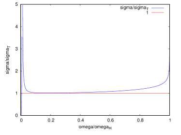
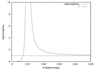
Figure 1: $\sigma(\omega)$ for $a\equiv\frac{4}{3\pi}r_{0,r}\omega_{H}=0.1$ and $b\equiv\frac{\Omega_{r}}{\omega_{H}}=0.01$. $\sigma(\omega)$ vanishes at $\omega=\omega_{H}$; the peak just below $\omega=\omega_{H}$ is an artifact of the sharp cutoff. The figure on the right is magnified for small $\omega$

V What is wrong with the naive continuum limit

To recapitulate, we have shown that the renormalized propagator $G_{r}(\omega^{2}+i\epsilon)$ depends on three parameters: $\Omega_{r}$ giving the resonance frequency, $r_{0,r}$ giving the Thomson cross section, and $\omega_{H}$ giving the high frequency cutoff of the photons. The photon scattering cross section at high frequencies depends on $\omega_{H}$ as given by (53).

Now, (34) tells us that the model is not renormalizable since $\omega_{H}$ cannot be taken to infinity. But if we examine the renormalized propagator given by (31), we find

$$G_{r}(\omega^{2}+i\epsilon)=\frac{1}{\omega^{2}-\Omega_{r}^{2}+\frac{2}{3\pi}r_{0,r}\omega^{3}\left(\ln\frac{\omega_{H}-\omega}{\omega_{H}+\omega}+i\pi\right)}$$ (54)

has a naive limit

$$\lim_{\omega_{H}\to+\infty}G_{r}(\omega^{2}+i\epsilon)=\frac{1}{\omega^{2}-\Omega_{r}^{2}+\omega^{3}\frac{i\pi}{2}\frac{4}{3\pi}r_{0,r}}\,.$$ (55)

What is wrong with this limit?

Let us examine the limit on the negative axis of $\omega^{2}$. At $\omega^{2}=-k^{2}<0$ we find

$$\frac{1}{G_{r}(-k^{2})} =-k^{2}-\Omega_{r}^{2}+k^{4}\frac{4}{3\pi}r_{0,r}\int_{0}^{\infty}d\omega^{\prime}\,\frac{1}{k^{2}+\omega^{\prime}\,{}^{2}}$$

$$=-k^{2}-\Omega_{r}^{2}+k^{3}\frac{2}{3}r_{0,r}\,.$$ (56)

This has a zero at $k=k_{t}\simeq\frac{3}{2r_{0,r}}+\frac{2}{3}r_{0,r}\Omega_{r}^{2}>0$, where

$$\frac{d}{dk}\frac{1}{G(-k^{2})}\Big{|}_{k=k_{t}}=\frac{2k_{t}}{r_{t}}>0\,.$$ (57)

(The positive constant $r_{t}$ is determined shortly.) This implies

$$\frac{1}{G_{r}(-k^{2})}\simeq\frac{2k_{t}}{r_{t}}(k-k_{t})\Longrightarrow G_{r}(-k^{2})\simeq\frac{r_{t}}{2k_{t}(k-k_{t})}\simeq\frac{-r_{t}}{-k^{2}+k_{t}^{2}}\,.$$ (58)

Hence, the propagator $G_{r}(\omega^{2}+i\epsilon)$ has a tachyon pole at $\omega^{2}=-k_{t}^{2}<0$, and the negative residue $-r_{t}$ at the pole implies a negative probability.

The spectral representation becomes

$$G_{r}(\omega^{2}+i\epsilon)=-\frac{r_{t}}{\omega^{2}+k_{t}^{2}}+\int_{0}^{\infty}\frac{ds}{\pi}\frac{s^{4}\frac{4}{3\pi}r_{0,r}}{\left(s^{2}-\Omega_{r}^{2}\right)^{2}+s^{6}\left(\frac{2r_{0,r}}{3}\right)^{2}}\frac{1}{\omega^{2}-s^{2}+i\epsilon}\,.$$ (59)

The sum rule gives the residue of the tachyon pole as

$$r_{t} =\int_{0}^{\infty}\frac{ds}{\pi}\frac{s^{4}\frac{4}{3\pi}r_{0,r}}{\left(s^{2}-\Omega_{r}^{2}\right)^{2}+s^{6}\left(\frac{2r_{0,r}}{3}\right)^{2}}$$

$$=\frac{2}{\pi^{2}}\int_{0}^{\infty}dx\,\frac{x^{4}}{\left(x^{2}-\left(\frac{2}{3}r_{0,r}\Omega_{r}\right)^{2}\right)^{2}+x^{6}}\,.$$ (60)

This is discontinuous at $\frac{2}{3}r_{0,r}\Omega_{r}=0$; for small $r_{0,r}\Omega_{r}\ll 1$, $r_{t}\simeq\frac{2}{\pi}$, but $r_{t}=\frac{1}{\pi}$ at $r_{0,r}=0$. We plot $\pi r_{t}$ for $0.001<\frac{2}{3}r_{0,r}\Omega_{r}<1$ in Fig. 2.

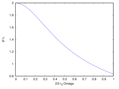
Figure 2: The residue of the tachyon pole is $-\pi r_{t}$. $\pi r_{t}$ is converging toward $2$ as $\frac{2}{3}r_{0,r}\Omega_{r}\to 0+$, though $\pi r_{t}=1$ strictly at zero

Now, what is wrong with the tachyon? The tachyon pole in $G(\omega^{2}+i\epsilon)$ implies the presence of a negative norm state with purely imaginary energy $\mp ik_{t}$. This is a clear violation of unitarity of the theory. In Appendix we explain a little more about the tachyon: we can trace its origin to a negative sign of the kinetic term in the lagrangian.

VI Smooth cutoff

Instead of introducing a sharp cutoff $\omega_{H}$ we may introduce a smooth positive cutoff function $K(\omega)$ that decays smoothly as $\omega\to+\infty$. As we will see, the physics at frequencies sufficiently smaller than $\omega_{H}$ does not depend on which cutoff scheme we use. This is universality.

Eq. (19) is replaced by

$$\frac{1}{G(\omega^{2}+i\epsilon)}=\omega^{2}-\Omega^{2}-\omega^{2}\frac{4}{3\pi}r_{0}\int_{0}^{\infty}d\omega^{\prime}\,K(\omega^{\prime})\frac{\omega^{\prime}\,{}^{2}}{\omega^{2}-\omega^{\prime}\,{}^{2}+i\epsilon}\,,$$ (61)

where $K(\omega)=1$ for low frequencies, but it decays fast enough as $\omega\to\infty$. (See Fig. 3.)

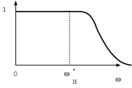
Figure 3: Cutoff function $K(\omega)$ is $1$ for low frequencies

We obtain

$$\frac{1}{G(\omega^{2}+i\epsilon)}=\left(1+\Delta z\right)\omega^{2}-\Omega^{2}-\omega^{4}\frac{4}{3\pi}r_{0}\int_{0}^{\infty}d\omega^{\prime}\,K(\omega^{\prime})\frac{1}{\omega^{2}-\omega^{\prime}\,{}^{2}+i\epsilon}\,,$$ (62)

where we have defined

$$\Delta z\equiv\frac{4r_{0}}{3\pi}\int_{0}^{\infty}d\omega^{\prime}K(\omega^{\prime})>0\,.$$ (63)

As in Sec. III we introduce renormalized quantities as follows:

$$\Omega_{r}^{2} \equiv\frac{\Omega^{2}}{1+\Delta z}\,,$$ (64a)

$$r_{0,r} \equiv\frac{r_{0}}{1+\Delta z}\,,$$ (64b)

$$G_{r}(\omega^{2}+i\epsilon) \equiv\left(1+\Delta z\right)G(\omega^{2}+i\epsilon)\,,$$ (64c)

so that

$$\frac{1}{G_{r}(\omega^{2}+i\epsilon)}=\omega^{2}-\Omega_{r}^{2}-\omega^{4}\frac{4}{3\pi}r_{0,r}\int_{0}^{\infty}d\omega^{\prime}\,K(\omega^{\prime})\frac{1}{\omega^{2}-\omega^{\prime}\,{}^{2}+i\epsilon}\,.$$ (65)

(63) and (64b) imply that $a_{K}$ defined below is less than $1$:

$$a_{K}\equiv\frac{4}{3\pi}r_{0,r}\int_{0}^{\infty}d\omega^{\prime}\,K(\omega^{\prime})=\frac{\Delta z}{1+\Delta z}<1\,.$$ (66)

Defining

$$b_{\omega}\equiv\omega^{2}-\Omega_{r}^{2}-\omega^{4}\frac{4}{3\pi}r_{0,r}\int_{0}^{\infty}d\omega^{\prime}\,K(\omega^{\prime})\mathbf{P}\frac{1}{\omega^{2}-\omega^{\prime}\,{}^{2}}$$ (67)

for $\omega>0$, we obtain

$$G_{r}(\omega^{2}+i\epsilon)=\frac{1}{b_{\omega}+\omega^{4}\frac{4}{3\pi}r_{0,r}K(\omega)\frac{i\pi}{2\omega}}\,.\quad(\omega>0)$$ (68)

As in Sec. III we can obtain a spectral representation of $G_{r}$:

$$G_{r}(\omega^{2}+i\epsilon)=\int_{0}^{\infty}ds\,\rho(s)\frac{1}{\omega^{2}-s+i\epsilon}\,,$$ (69)

where the positive spectral function is given by

$$\rho(s) =\frac{2s}{\pi}(-)\Im G_{r}(s^{2}+i\epsilon)$$

$$=\frac{s^{4}\frac{4}{3\pi}r_{0,r}K(s)}{b_{s}^{2}+\left(s^{4}\frac{4}{3\pi}r_{0,r}K(s)\frac{\pi}{2s}\right)^{2}}\,.$$ (70)

To obtain a sum rule for $\rho(s)$, we must make sure that $G_{r}(\omega^{2})$, defined by (65) for the entire complex plane of $\omega^{2}$, has no pole on the negative real axis. There is no such pole because at $\omega^{2}=-k^{2}<0$ we obtain

$$-k^{2}\left(1-\frac{4}{3\pi}r_{0,r}\int_{0}^{\infty}d\omega^{\prime}\,K(\omega^{\prime})\frac{k^{2}}{k^{2}+\omega^{\prime}\,{}^{2}}\right)-\Omega_{r}^{2}<0$$ (71)

thanks to (66). The asymptotic behavior

$$G_{r}(\omega^{2}+i\epsilon)\overset{\omega^{2}\to\infty}{\longrightarrow}\frac{1}{1-a_{K}}\frac{1}{\omega^{2}}$$ (72)

then implies a sum rule analogous to (43):

$$\int_{0}^{\infty}ds\,\rho(s)=\frac{1}{1-a_{K}}\,.$$ (73)

Accordingly, the cross section $\sigma(\omega)=2\pi^{2}r_{0,r}\rho(\omega)$ satisfies

$$\int_{0}^{\infty}d\omega\,\sigma(\omega)=2\pi^{2}r_{0,r}\frac{1}{1-a_{K}}\,,$$ (74)

analogous to (50).

We would like to find the approximate behavior of the cross section for $\omega$ small compared with a cutoff scale. Suppose $K(\omega)=1$ for $\omega<\omega^{\prime}_{H}$, where $\omega^{\prime}_{H}$ is much larger than $\Omega_{r}$. We then obtain, for $0<\omega<\omega^{\prime}_{H}$,

$$\int_{0}^{\infty}d\omega^{\prime}\,K(\omega^{\prime})\frac{1}{\omega^{2}-\omega^{\prime}\,{}^{2}+i\epsilon}$$

$$=\int_{0}^{\omega^{\prime}_{H}}d\omega^{\prime}\,\frac{1}{\omega^{2}-\omega^{\prime}\,{}^{2}+i\epsilon}+\int_{\omega^{\prime}_{H}}^{\infty}d\omega^{\prime}\,K(\omega^{\prime})\frac{1}{\omega^{2}-\omega^{\prime}\,{}^{2}}$$

$$=\frac{1}{2\omega}\left(-\ln\frac{\omega^{\prime}_{H}-\omega}{\omega^{\prime}_{H}+\omega}-i\pi\right)+\int_{\omega^{\prime}_{H}}^{\infty}d\omega^{\prime}\,K(\omega^{\prime})\frac{1}{\omega^{2}-\omega^{\prime}\,{}^{2}}\,.$$ (75)

Expanding in powers of $\frac{\omega}{\omega^{\prime}_{H}}$, we obtain

$$\int_{0}^{\infty}d\omega^{\prime}\,K(\omega^{\prime})\frac{1}{\omega^{2}-\omega^{\prime}\,{}^{2}+i\epsilon}\simeq-\frac{i\pi}{2\omega}+\frac{1}{\omega^{\prime}_{H}}-\int_{\omega^{\prime}_{H}}^{\infty}d\omega^{\prime}\,K(\omega^{\prime})\frac{1}{\omega^{\prime}\,{}^{2}}\,.$$ (76)

Hence, for $\omega\ll\omega^{\prime}_{H}$, we can approximate

$$b_{\omega}\simeq\omega^{2}-\Omega_{r}^{2}-\omega^{4}\frac{4}{3\pi}r_{0,r}\left(\frac{1}{\omega^{\prime}_{H}}-\int_{\omega^{\prime}_{H}}^{\infty}d\omega^{\prime}\,K(\omega^{\prime})\frac{1}{\omega^{\prime}\,{}^{2}}\right)\,.$$ (77)

We can identify

$$\frac{1}{\omega_{H}}\equiv\frac{1}{\omega^{\prime}_{H}}-\int_{\omega^{\prime}_{H}}^{\infty}d\omega^{\prime}\,K(\omega^{\prime})\frac{1}{\omega^{\prime}\,{}^{2}}$$ (78)

with the cutoff frequency of the sharp cutoff. As long as $\omega\ll\omega_{H}$, the smooth cutoff gives the same propagator, hence the same cross section, as the sharp cutoff with the same $\omega_{H}$. We note that $\omega_{H}$ given by (78) depends only on the cutoff function $K$ but not on the particular choice of $\omega^{\prime}_{H}$. We show the cross section $\sigma(\omega)$ for three smooth cutoff functions and a sharp cutoff corresponding to the same $\omega_{H}$. (Fig. 4) They seem to agree even up to relatively large $\omega$.

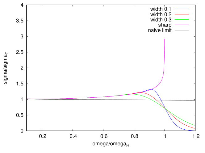
Figure 4: $\sigma(\omega)$ for $0.1<\frac{\omega}{\omega_{H}}<1.2$ with four choices of cutoff. The “width” of a smooth cutoff is the width of the region where $K$ drops from $1$ to almost $0$. The four schemes agree for $\frac{\omega}{\omega_{H}}<0.8$. We also show the “naive limit” discussed in Sec. V

In conclusion, the cross section for $\omega$ sufficiently smaller than $\omega_{H}$ is independent of a particular choice of the cutoff scheme. The sum rule (74) for the cross section, however, depends on the cutoff scheme.

VII Conclusion

In this paper we have reconsidered the familiar model of a charged harmonic oscillator interacting with the radiation field in the electric dipole approximation, and examined the question of renormalizability.

The lagrangian (9) with two parameters $\Omega,r_{0}=\frac{e^{2}}{4\pi m}$ is naively renormalizable via the renormalization of the wave function and the parameters. But we have identified the problem of a tachyon that spoils unitarity of the model. The frequency cutoff $\omega_{H}$ must be kept finite, and it can be considered as the third parameter of the model besides the renormalized parameters $\Omega_{r}$ and $r_{0,r}$, defined by (25, 26). We have shown that for frequencies sufficiently smaller than $\omega_{H}$, the photon scattering cross section depends only on the three parameters, not sensitive to the precise way the cutoff is introduced. In this sense $\omega_{H}$ is analogous to the coupling constant of many renormalizable theories in four dimensions, such as $\phi^{4}$ and QED, whose renormalizability is only perturbative. The problem with tachyons is well known in the renormalization of the Lee model Lee (1954) and the large $N$ limit of the $\phi^{4}$ theory Coleman et al. , both in four dimensions. The tachyons are absent as long as the UV cutoff is kept finite in both cases.

*

Appendix A The origin of a tachyon

We would like to show that the tachyon we have found in the naive continuum limit can be traced to a negative kinetic term in the lagrangian. In terms of renormalized parameters the lagrangian (9) of the model is given by

$$L=\frac{1}{2}(1-a)\frac{d}{dt}\vec{X}_{r}\cdot\frac{d}{dt}\vec{X}_{r}-\Omega_{r}^{2}\frac{1}{2}\vec{X}_{r}^{2}+\sqrt{4\pi r_{0,r}}\,\frac{d}{dt}\vec{X}_{r}\cdot\sqrt{\frac{2}{V}}\sum_{n}\vec{\epsilon}_{n}\phi_{n}+\sum_{n}\frac{1}{2}\left(\left(\partial_{t}\phi_{n}\right)^{2}-\omega_{n}^{2}\phi_{n}^{2}\right)\,,$$ (79)

where the parameter $a$ is given by

$$a\equiv\frac{4}{3\pi}r_{0,r}\omega_{H}\,.$$

Given $r_{0,r}$, disregarding the inequality (33), we may increase $\omega_{H}$ beyond the limit (34). For $a>1$, the kinetic term is negative, and we are not surprised to find that the propagator acquires a tachyon with a negative residue.

To be more precise, on the negative axis of $\omega^{2}$, the inverse of the renormalized propagator $G_{r}(\omega^{2}+i\epsilon)$ is given by

$$\frac{1}{G_{r}(-k^{2})}=-k^{2}-\Omega_{r}^{2}+k^{3}\frac{4r_{0,r}}{3\pi}\arctan\frac{\omega_{H}}{k}\,.$$ (80)

In the limit $\omega_{H}\to+\infty$, this gives (56) considered in Sec. V. We can show that this propagator has a simple pole at $k^{2}=k_{t}^{2}$ with a negative residue $-\pi r_{t}$. For $a$ slightly larger than $1$, we obtain approximately

$$\frac{k_{t}}{\omega_{H}}\simeq\sqrt{\frac{\frac{a}{3}+\left(\frac{\Omega_{r}}{\omega_{H}}\right)^{2}}{a-1}}\,,\quad r_{t}\simeq\frac{1}{a-1}\,.$$ (81)

We have discussed the limit $a\to+\infty$ in Sec. V. As $a$ increases toward $1$, the bound state pole $\Omega_{b}^{2}$, discussed in Sec. III, approaches infinity. As we take $a$ across $1$, the pole returns as a tachyon pole $-k_{t}^{2}$, and it moves toward the pole found in Sec. V as we increase $a$ further.

References

Weisskopf and Wigner (1930a)V. Weisskopf and Eugene P. Wigner, “Calculation of
the natural brightness of spectral lines on the basis of Dirac’s theory,” Z. Phys. 63, 54–73 (1930a).
Weisskopf and Wigner (1930b)V. Weisskopf and Eugene P. Wigner, “Over the
natural line width in the radiation of the harmonic oscillator,” Z.
Phys. 65, 18–29
(1930b).