Reduction of Chemical Reaction Networks with Approximate Conservation Laws

Abstract

Model reduction of fast-slow chemical reaction networks based on the quasi-steady state approximation fails when the fast subsystem has first integrals. We call these first integrals approximate conservation laws. In order to define fast subsystems and identify approximate conservation laws, we use ideas from tropical geometry. We prove that any approximate conservation law evolves slower than all the species involved in it and therefore represents a supplementary slow variable in an extended system. By elimination of some variables of the extended system, we obtain networks without approximate conservation laws, which can be reduced by standard singular perturbation methods. The field of applications of approximate conservation laws covers the quasi-equilibrium approximation, well known in biochemistry. We discuss reductions of slow-fast as well as multiple timescale systems. Networks with multiple timescales have hierarchical relaxation. At a given timescale, our multiple timescale reduction method defines three subsystems composed of (i) slaved fast variables satisfying algebraic equations, (ii) slow driving variables satisfying reduced ordinary differential equations, and (iii) quenched much slower variables that are constant. The algebraic equations satisfied by fast variables define chains of nested normally hyberbolic invariant manifolds. In such chains, faster manifolds are of higher dimension and contain the slower manifolds. Our reduction methods are introduced algorithmically for networks with monomial reaction rates and linear, monomial or polynomial approximate conservation laws. We propose symbolic algorithms to reshape and rescale the networks such that geometric singular perturbation theory can be applied to them, test the applicability of the theory, and finally reduce the networks. As a proof of concept, we apply this method to a model of the TGF-$\beta$ signaling pathway.

Keywords: Model order reduction, chemical reaction networks, singular perturbations, multiple timescales, tropical geometry.

1 Introduction

The study of chemical reaction networks (CRN) was motivated by important applications in physics and chemistry, concerning models of non-equilibrium thermodynamics [48], catalytic reactions [61], combustion [53], etc. More recently, CRNs were used to model cell and tissue physiology [55] needed for the understanding of the fundamental mechanisms of living systems and for fighting disease.

Chemical reaction networks can be characterized by reaction stoichiometry and reaction rates [2]. Stoichiometry tells us how many molecules of each species are consumed and produced in a reaction. For instance, the reaction $A_{1}+A_{2}\rightarrow A_{3}$ consumes one molecule of each $A_{1}$ and $A_{2}$ and produces one molecule of $A_{3}$. A useful construct is the stoichiometric matrix $\boldsymbol{S}$ in which each column represents the net numbers of molecules of each species produced by a particular reaction. A three species CRN made of the reactions $A_{1}+A_{2}\rightarrow A_{3}$ and $A_{1}+A_{1}\rightarrow A_{1}$ has the stoichiometric matrix

$$\boldsymbol{S}=\begin{pmatrix}-1&-1\\ -1&0\\ 1&0\end{pmatrix}.$$

With each reaction we also associate a positive function of species concentrations, called reaction rate, representing the number of occurrences of the reaction per unit time and volume. In this paper we assume that reaction rates are monomials. Therefore, the deterministic kinetics of CRNs is described by sets of polynomial ordinary differential equations. For instance, if the reaction rates in the above example are $R_{1}=k_{1}x_{1}x_{2}$ and $R_{2}=k_{2}x_{1}^{2}$, the CRN kinetics is described by $\dot{x}_{1}=-k_{1}x_{1}x_{2}-\frac{1}{2}k_{2}x_{1}^{2}$, $\dot{x}_{2}=-k_{1}x_{1}x_{2}$ and $\dot{x}_{3}=k_{1}x_{1}x_{2}$.

A lot of effort has been dedicated to studying the behavior of mass-action networks [14]. In such networks, the probability that two species react is proportional to their abundances, and therefore the reaction rates are monomials in the concentrations of reactant species with exponents equal to the number of molecules entering the reaction. The above example is of this type, but will no longer be of this type if $R_{1}$ is changed to $k_{1}x_{1}x_{2}^{2}$, for instance. This constraint leads to algebraic properties exploited in chemical reaction network theory (CRNT), which has been initiated by Horn, Jackson and Feinberg [15, 14]. In order to cover more general models, we do not impose the mass action constraint on the reaction rates. Instead, to avoid that some species become negative as a result of the CRN kinetics, we use a weaker constraint: if a reaction consumes a species, then its rate is proportional to a strictly positive power of the concentration of this species. In spite of significant progress towards elucidating the properties of CRNs, important models are left aside because of their size and complexity of their dynamics. For such examples, algorithmic model reduction, which transforms complex networks into simpler ones that can be more easily analysed, becomes a necessity. A few attempts of developing model reduction algorithms used concepts of CRNT such as complex balance [44, 17], but they were limited to networks functioning at the steady state or based on ad hoc identification of the balanced complexes. Model reduction methods based on the theory of singular perturbations, employing concepts such as the intrinsic low dimensional manifold or quasi-steady state reduction, are often used in chemistry and systems biology [54, 21]. However, these methods lack general algorithms for finding appropriate small parameters and scalings, needed for the quasi-steady state reduction, and are limited to two time-scales (slow-fast systems).

Recently, we proposed a symbolic method for algorithmic reduction of chemical reaction networks with multiple (more than two) timescales [27]. This method combines tropical geometry ideas for identifying the time and concentration scales [46, 39], dominance principles based on comparison of orders of magnitude [23, 40, 24] and singular perturbation results [18, 8] to justify the reduction. For a given timescale, the method defines three subsystems: a slaved equilibrated subsystem, a driving evolving subsystem and a quenched subsystem. The variables of the slaved subsystem satisfy quasi-steady equations, defined as equilibria of the fast truncated ODEs in which all the remaining variables are considered fixed. The entire construction requires the hyperbolicity of the quasi-steady state, which is needed in the classical geometrical singular perturbation theory of Fenichel [18]. Although general in its implementation, this reduction method fails in a number of cases. A major cause of failure is the degeneracy of the quasi-steady state, when the fast dynamics has a continuous variety of steady states. Typically, this happens when the fast truncated ODEs have first integrals, i.e. quantities that are conserved on any trajectory, whose values depend on the initial conditions. The quasi-steady states are no longer hyperbolic, because the Jacobian matrix of the fast part of the dynamics is in this case singular. This type of singular perturbations, called critical, is known since the work of Vasil’eva and Butuzov in the 70’s [57], but its origins can be traced back to the early theory of enzymatic reactions, as quasi-equilibrium is an instance of critical singular perturbations. Vasil’eva and Butuzov [57] propose asymptotic expansions of the solutions of singularly perturbed systems in the critical case based on their method of boundary series, which are two timescale expansions. Their method works in the case when the problem has rigorously two timescales, but can not be applied in the case when there are more than two timescales. We show in this paper that critical singular perturbations may have more timescales than are apparent after rescaling parameters and variables. We also provide algorithmic methods to compute these extra timescales that correspond to approximate conservation laws.

Exact conservation laws, i.e. first integrals of the full dynamics, were already used for model order reduction. If such quantities exist, the model can be reduced by eliminating a number of variables and equations equal to the number of independent conservation laws [29, 32]. In the present work, we introduce the approximate conservation laws that are quantities conserved by the fast dynamics. In models with multiple timescales, approximate conservation laws provide extra slow variables. Model reduction takes place by elimination of the fast variables. We thus provide algorithmic reduction methods covering the case of non-hyperbolic fast dynamics with conservation. Our algorithms are inspired from the well-known quasi-equilibrium approximation [24, 41]. Contrary to the quasi-equilibrium approximation that uses only linear approximate conservation laws, here we are also exploiting non-linear conserved quantities. Similar ideas were developed in [49, 9, 3], but without a full algorithmic solution. Like in [27] we use tropical geometry to find appropriate time and concentration scales.

The topic of conservation laws has a broad interest and its relation to symmetry was widely studied in classical and quantum mechanics (see Noether’s theorems [36]). Referring to the broad range of phenomena in physics, from nuclear forces to gravitation, having near symmetry, R. Feynman concludes that “God made the laws only nearly symmetrical so that we should not be jealous of His perfection” [19]. Approximate continuous symmetries (Lie-Bäcklund symmetries) were studied for differential equations with or without a Lagrangian (see [4] and [26], respectively). Beyond their utility in the theory of regular and singular perturbations, exact and approximate symmetries can be used to gain insight into the dynamics of complex chemical reaction networks. Approximate conservation laws, valid for certain concentrations and not valid for other concentrations of biochemical species, imply that the same biochemical system can have multiple behaviors depending on the internal or external stimuli. In biology, “imperfect” conservation allows living systems to be flexible, to evolve and adapt to changes of the environment. This also leads to multiple dynamical phenomena: slow metastable states, bifurcations in the fast dynamics of the system and itineracy when the system switches from one metastable state to another [23, 3, 38].

The structure of this paper is as follows. Section 2 introduces the class of models we are dealing with. These are systems of ODEs whose r.h.s. are integer coefficient polynomials in species concentrations and reaction rate constants. Theorem 1 shows that these models are always endowed with a stoichiometric matrix. Section 3 introduces the concept of exact and approximate conservation laws, without methods for computing them. The methods for symbolic computation of approximate conservation laws are presented in [10]. Section 4 introduces our reduction method based on tropically constrained formal scalings and approximate conservation laws. An important result here is that approximate conservation laws are always slower than all the species involved in their structure. This implies that they can be used as new, unconditionally slow variables, providing robust reductions. In 6 we illustrate the method via a case study from molecular biology of intracellular signal transduction.

2 Models

In this paper we consider CRNs with $n$ species $A_{1},\ldots,A_{n}$, whose concentrations $\boldsymbol{x}=(x_{1},\ldots,x_{n})$ follow a system of ODEs of the form

$$\dot{x}_{1}=f_{1}(\boldsymbol{k},\boldsymbol{x}),\,\dots,\,\dot{x}_{n}=f_{n}(\boldsymbol{k},\boldsymbol{x}),$$ (1)

where

$$f_{i}(\boldsymbol{k},\boldsymbol{x})=\sum_{j=1}^{r}S_{ij}k_{j}\boldsymbol{x}^{\boldsymbol{\alpha}_{j}}\in\mathbb{Z}[\boldsymbol{k},\boldsymbol{x}]=\mathbb{Z}[k_{1},\dots,k_{r},x_{1},\dots,x_{n}].$$

The monomials $\boldsymbol{x}^{\boldsymbol{\alpha}_{j}}=x_{1}^{\alpha_{j1}}\ldots x_{n}^{\alpha_{j_{n}}}$ appearing in the right hand sides of (1) are defined by $r$ multi-indices $\boldsymbol{\alpha}_{j}=(\alpha_{j1},\ldots,\alpha_{jn})\in\mathbb{N}^{n}$ and for each monomial the variable $k_{j}$ represents a rate constant. The variables $\boldsymbol{k}=(k_{1},\dots,k_{r})$ take values in $\mathbb{R}_{>0}^{r}$ and the integer coefficients $S_{ij}$ form a matrix $\boldsymbol{S}=(S_{ij})\in\mathbb{Z}^{n\times r}$, which is called the stoichiometric matrix. The concentration variables $\boldsymbol{x}=(x_{1},\ldots,x_{n})$ take values in $\mathbb{R}_{>0}^{n}$. For reasons that will become clear in Section 4.2 in Remark 16, we exclude zero concentrations. We denote the vector of right hand sides of (1) by

$$\boldsymbol{F}(\boldsymbol{k},\boldsymbol{x})=(f_{1}(\boldsymbol{k},\boldsymbol{x}),f_{2}(\boldsymbol{k},\boldsymbol{x}),\ldots,f_{n}(\boldsymbol{k},\boldsymbol{x}))^{\mathsf{T}}.$$

Mass action networks belong to this class of models. For a mass action reaction

$$\bar{\alpha}_{j1}A_{1}+\ldots+\bar{\alpha}_{jn}A_{n}\rightarrow\beta_{j1}A_{1}+\ldots+\beta_{jn}A_{n}$$

we have that $S_{ij}=\beta_{ji}-\bar{\alpha}_{ji}$ and that the reaction rate is $k_{j}\boldsymbol{x}^{\boldsymbol{\bar{\alpha}}_{j}}$, i.e. the stoichiometric coefficients $\boldsymbol{\bar{\alpha}}_{j}$ and the multi-indices $\boldsymbol{\alpha}_{j}$ coincide. But in general this must not be the case, meaning that the multi-indices $\boldsymbol{\alpha}_{j}$ and $\boldsymbol{\bar{\alpha}}_{j}$ in $S_{ij}=\beta_{ji}-\bar{\alpha}_{ji}$ and $k_{j}\boldsymbol{x}^{\boldsymbol{\alpha}_{j}}$ are not necessarily equal. In order to keep the positive orthant $\mathbb{R}_{>0}^{n}$ invariant, we consider that whenever a reaction consumes a species, its rate tends to zero when the concentration of this species approaches zero. This is equivalent to

Condition 1.

$\alpha_{ji}>0$ for all $i,j$ such that $S_{ij}<0$.

The condition 1 is automatically satisfied by mass action reactions, but covers also truncated ODEs systems introduced in Section 3.1 and used in Section 4.

3 Approximate Conservation Laws

3.1 A Classical Example and some Definitions

Example 2.

Let us consider the irreversible Michaelis-Menten mechanism that is paradigmatic for enzymatic reactions. We choose rate constants corresponding to the so-called quasi-equilibrium, studied by Michaelis and Menten. The reaction network for this model is

$$S+E\underset{k_{2}}{\overset{k_{1}}{\rightleftharpoons}}ES\overset{k_{3}\delta}{\longrightarrow}E+P,$$

where $S$ is a substrate, $E$ is an enzyme, $ES$ is an enzyme-substrate complex and $k_{1}$, $k_{2}$, $k_{3}$ are rate constants. Here $0<\delta<1$ is a small positive scaling parameter, indicating that the third rate constant is small.

According to mass-action kinetics, the concentrations $x_{1}=[S]$, $x_{2}=[ES]$ and $x_{3}=[E]$ satisfy the system of ODEs

$$\dot{x_{1}} = -k_{1}x_{1}x_{3}+k_{2}x_{2},$$

$$\dot{x_{2}} = k_{1}x_{1}x_{3}-k_{2}x_{2}-\delta k_{3}x_{2},$$

$$\dot{x_{3}} = -k_{1}x_{1}x_{3}+k_{2}x_{2}+\delta k_{3}x_{2}.$$ (2)

We consider the truncated system of ODEs

$$\dot{x_{1}} = -k_{1}x_{1}x_{3}+k_{2}x_{2},$$

$$\dot{x_{2}} = k_{1}x_{1}x_{3}-k_{2}x_{2},$$

$$\dot{x_{3}} = -k_{1}x_{1}x_{3}+k_{2}x_{2},$$ (3)

which is obtained by setting $\delta=0$ in (2). The truncated system (2) describes the dynamics of the model on fast timescales of order ${O}(\delta^{0})$.

The steady state of the fast dynamics is obtained by equating to zero the r.h.s. of (2). The resulting condition is called quasi-equilibrium (QE) because it means that the complex formation rate $k_{1}x_{1}x_{3}$ is equal to the complex dissociation rate $k_{2}x_{2}$. In other words, the reversible reaction

$$S+E\underset{k_{2}}{\overset{k_{1}}{\rightleftharpoons}}ES$$

functions at equilibrium. The QE condition is reached only at the end of the fast dynamics and is satisfied with a precision of order ${O}(\delta)$ during the slow dynamics [24]. Because of its approximate validity and purely kinetic origin, QE is different from the similar concept of detailed balance [7].

We introduce the linear combinations of variables $x_{4}=x_{1}+x_{2}$ and $x_{5}=x_{2}+x_{3}$ corresponding to the total substrate and total enzyme concentrations, respectively. Addition of the last two equations of (2) leads to $\dot{x}_{5}=0$, which means that for solutions of the full system $x_{5}$ is constant for all times. We will call such a quantity an exact conservation law.

Addition of the first two and the last two equations of (2) lead to $\dot{x}_{4}=0$ and $\dot{x}_{5}=0$. This means that $x_{4}$ is constant for solutions of the truncated dynamics, valid at short times $t={O}(\delta^{0})$ and is not constant at larger times $t={O}(\delta^{-1})$. We call such a quantity an approximate conservation law. The quantity $x_{5}$ is both an exact and approximate conservation law.

More generally, let us consider system (1). This model depends on the parameters $\boldsymbol{k}=(k_{1},\dots,k_{r})$. After rescaling it by powers of a scaling parameter $\delta$ with $0<\delta<1$, it becomes (for details see Section 4.1)

$$\dot{\bar{x}}_{1} = \delta^{b_{1}}\big{(}\bar{f}_{1}^{(1)}(\boldsymbol{\bar{k}},\boldsymbol{\bar{x}})+\delta^{b^{\prime}_{1}}\bar{f}_{1}^{(2)}(\boldsymbol{\bar{k}},\boldsymbol{\bar{x}},\delta)\big{)},$$

$$\vdots$$

$$\dot{\bar{x}}_{n} = \delta^{b_{n}}\big{(}\bar{f}_{n}^{(1)}(\boldsymbol{\bar{k}},\boldsymbol{\bar{x}})+\delta^{b^{\prime}_{n}}\bar{f}_{n}^{(2)}(\boldsymbol{\bar{k}},\boldsymbol{\bar{x}},\delta)\big{)},$$ (4)

where $b^{\prime}_{i}>0$. The rescaled model (3.1) is rewritten in rescaled variables $\boldsymbol{\bar{x}}=(\bar{x}_{1},\dots,\bar{x}_{n})$ and depends on the rescaled parameters $\boldsymbol{\bar{k}}=(\bar{k}_{1},\dots,\bar{k}_{r})$.

The functions $\bar{f}_{i}^{(2)}(\boldsymbol{\bar{k}},\boldsymbol{\bar{x}},\delta)$ are infinitely differentiable and their first derivatives in $\delta$ vanish at $\delta=0$. We also have

$$f_{i}(\boldsymbol{k},\boldsymbol{x})=\delta^{b_{i}}\big{(}\bar{f}_{i}^{(1)}(\boldsymbol{\bar{k}},\boldsymbol{\bar{x}})+\delta^{b^{\prime}_{i}}\bar{f}_{i}^{(2)}(\boldsymbol{\bar{k}},\boldsymbol{\bar{x}},\delta)\big{)}.$$

For small $\delta$ and $b_{i}^{\prime}>0$ the terms in $\delta^{b^{\prime}_{i}}\bar{f}_{i}^{(2)}(\boldsymbol{\bar{k}},\boldsymbol{\bar{x}},\delta)$ are dominated by the terms in $\bar{f}_{i}^{(1)}(\boldsymbol{\bar{k}},\boldsymbol{\bar{x}})$. This justifies to introduce the truncated system as the system of ODEs obtained by keeping only the lowest order dominant terms in (3.1), namely

$$\dot{x}_{1}=f_{1}^{(1)}(\boldsymbol{k},\boldsymbol{x}),\,\ldots,\,\dot{x}_{n}=f_{n}^{(1)}(\boldsymbol{k},\boldsymbol{x}),$$ (5)

where $f_{i}^{(1)}(\boldsymbol{k},\boldsymbol{x})=\delta^{b_{i}}\bar{f}_{i}^{(1)}(\boldsymbol{\bar{k}},\boldsymbol{\bar{x}})$ for all $1\leq i\leq n$.

Definition 3.

 

1. A function $\phi(\boldsymbol{x})$ is an exact conservation law, unconditionally on the parameters, if it is a first integral of the full system (1), i.e. if

   $$\sum_{i=1}^{n}\frac{\partial\phi}{\partial x_{i}}(\boldsymbol{x})f_{i}(\boldsymbol{k},\boldsymbol{x})=0$$

   for all $\boldsymbol{k}\in\mathbb{R}_{>0}^{r}$, $\boldsymbol{x}\in\mathbb{R}_{>0}^{n}$.

2. A function $\phi(\boldsymbol{x})$ is an approximate conservation law, unconditionally on the parameters, if it is a first integral of the truncated system (5), i.e. if

   $$\sum_{i=1}^{n}\frac{\partial\phi}{\partial x_{i}}(\boldsymbol{x})f_{i}^{(1)}(\boldsymbol{k},\boldsymbol{x})=0$$

   for all $\boldsymbol{k}\in\mathbb{R}_{>0}^{r}$, $\boldsymbol{x}\in\mathbb{R}_{>0}^{n}$.

3. An exact (approximate) conservation law of the form $c_{1}x_{1}+\dots+c_{n}x_{n}$ with coefficients $c_{i}\in\mathbb{R}$ is called an exact (approximate) linear conservation law. If $c_{i}\geq 0$ for $1\leq i\leq n$, the linear conservation law is called semi-positive.

4. An exact (approximate) conservation law of the form $x_{1}^{m_{1}}\cdots x_{n}^{m_{n}}$ with $m_{i}\in\mathbb{Z}$ is called an exact (approximate) rational monomial conservation law. If $m_{i}\in\mathbb{Z}_{+}$ for $1\leq i\leq n$, the conservation law is called monomial. For simplicity, in this paper, we will call both types monomial.

5. An exact (approximate) conservation law of the form $\sum_{i=1}^{s}a_{i}x_{1}^{m_{1i}}\cdots x_{n}^{m_{ni}}$ with $m_{ji}\in\mathbb{Z}_{+}$ and $a_{i}\in\mathbb{R}$ is called an exact (approximate) polynomial conservation law.

Remark 4.

In the above definitions $\phi(\boldsymbol{x})$ does not contain $\boldsymbol{k}$, and exists for all admissible $\boldsymbol{k}$, which is a slight limitation. This condition facilitates the calculation of time scale orders needed for model reduction (see Section 4.4). Of course, some conservation laws may depend on $\boldsymbol{k}$, and/or exist only for special values of $\boldsymbol{k}$, but finding them and their existence conditions is generally a much more difficult problem. Parametric conservation laws are considered in our parallel paper [10]. From now on, for the sake of simplicity and when it is clear from the context, we will refer to the categories in ((a)) and ((b)) of Definition 3 as conservation law and approximate conservation law, respectively. Let us note that an approximate conservation law can also be exact.

Some variables may not appear in a conservation law $\phi(\boldsymbol{x})$. This means that in the case of a linear conservation law some coefficients $c_{i}$ may be zero, or in the case of a nonlinear conservation law some partial derivatives $\frac{\partial\phi}{\partial x_{i}}(\boldsymbol{x})$ may vanish. If $r$ is the number of all non-zero quantities $\frac{\partial\phi}{\partial x_{i}}(\boldsymbol{x})$, then we say that the conservation law depends on $r$ variables.

Definition 5.

An exact or approximate conservation law depending on $r$ variables is called simple if it can not be split into the sum or the product of two conservation laws such that at least one of them depends on a number $r^{\prime}$ of variables, with $1\leq r^{\prime}<r$.

Definition 6.

For $\boldsymbol{k}\in\mathbb{R}_{>0}^{r}$ a steady state $\boldsymbol{x}$ is a positive solution of $\boldsymbol{F}(\boldsymbol{k},\boldsymbol{x})=0$ and we denote the steady state variety by $\mathcal{S}_{\boldsymbol{k}}$. A steady state $\boldsymbol{x}$ is degenerate or non-degenerate if the Jacobian $D_{\boldsymbol{x}}\boldsymbol{F}(\boldsymbol{k},\boldsymbol{x})$ is singular or regular, respectively.

Degeneracy of steady states implies that $\mathcal{S}_{\boldsymbol{k}}$ is not discrete. Reciprocally, if the local dimension at a point $\boldsymbol{x}_{0}\in\mathcal{S}_{\boldsymbol{k}}$ is strictly positive, then $\boldsymbol{x}_{0}$ is degenerate (Theorem 10 of [10]).

Definition 7.

A set

$$\boldsymbol{\Phi}(\boldsymbol{x})=\left(\phi_{1}(\boldsymbol{x}),\ldots,\phi_{s}(\boldsymbol{x})\right)^{\mathsf{T}}$$

of exact conservation laws is called complete if the Jacobian matrix

$$\boldsymbol{J}_{\boldsymbol{F},\boldsymbol{\Phi}}(\boldsymbol{k},\boldsymbol{x})=D_{\boldsymbol{x}}(\boldsymbol{F}(\boldsymbol{k},\boldsymbol{x}),\boldsymbol{\Phi}(\boldsymbol{x}))^{\mathsf{T}}$$

has rank $n$ for any $\boldsymbol{k}\in\mathbb{R}_{>0}^{r}$, $\boldsymbol{x}\in\mathbb{R}_{>0}^{n}$ satisfying $\boldsymbol{F}(\boldsymbol{k},\boldsymbol{x})=0$. The set is called independent if the Jacobian matrix of $\boldsymbol{\Phi}(\boldsymbol{x})^{\mathsf{T}}$ with respect to $\boldsymbol{x}$ has rank $s$ for any $\boldsymbol{k}\in\mathbb{R}_{>0}^{r}$, $\boldsymbol{x}\in\mathbb{R}_{>0}^{n}$ such that $\boldsymbol{F}(\boldsymbol{k},\boldsymbol{x})=0$. In the case of a set $\boldsymbol{\Phi}(\boldsymbol{x})$ of approximate conservation laws completeness is defined with $\boldsymbol{F}(\boldsymbol{k},\boldsymbol{x})$ replaced by

$$\boldsymbol{F}^{(1)}(\boldsymbol{k},\boldsymbol{x})=\left(f_{1}^{(1)}(\boldsymbol{k},\boldsymbol{x}),\ldots,f_{n}^{(1)}(\boldsymbol{k},\boldsymbol{x})\right)^{\mathsf{T}}.$$

If a CRN has a complete set of conservation laws $\boldsymbol{\Phi}(\boldsymbol{x})$, then the set of positive solutions of $\boldsymbol{F}(\boldsymbol{k},\boldsymbol{x})=0$, $\boldsymbol{\Phi}(\boldsymbol{x})=\boldsymbol{c}_{0}$ is finite (see Proposition 12 of [10]).

Remark 8.

If the components of $\boldsymbol{\Phi}(\boldsymbol{x})$ are linear in $\boldsymbol{x}$ and comes from a stoichiometric matrix, the set

$$\{\boldsymbol{\Phi}(\boldsymbol{x})=\boldsymbol{c}_{0}\}\cap\mathbb{R}_{\geq 0}^{n}$$

is called stoichiometric compatibility class or reaction simplex [59, 15]. Stoichiometric compatibility classes of systems with complete sets of linear conservation laws contain a finite number of steady states (see Proposition 12 of [10]). We note that some authors call completeness of linear conservation laws non-degeneracy [16].

Remark 9.

Since our concern is the number of strictly positive solutions in $\boldsymbol{x}$ of the system $\boldsymbol{F}(\boldsymbol{k},\boldsymbol{x})=0$, $\boldsymbol{\Phi}(\boldsymbol{x})=\boldsymbol{c}_{0}$, in Definition 7 it would be more natural to consider the rank of $\boldsymbol{J}_{\boldsymbol{F},\boldsymbol{\Phi}}(\boldsymbol{k},\boldsymbol{x})$ on $\mathcal{S}_{\boldsymbol{k}}\cap\{\boldsymbol{\Phi}(\boldsymbol{x})=\boldsymbol{c}_{0}\}\cap\mathbb{R}_{>0}^{n}$. In fact, as this rank does not depend on $\boldsymbol{c}_{0}$, it is simpler and equivalent to impose its value on $\mathcal{S}_{\boldsymbol{k}}\cap\mathbb{R}_{>0}^{n}$.

Remark 10.

The independent linear conservation laws

$$\boldsymbol{\Phi}(\boldsymbol{x})=(x_{1}+x_{2},\,x_{2}+x_{3})$$

of Example 2 are complete. More precisely, the Jacobian of $(\boldsymbol{F}(\boldsymbol{x}),\boldsymbol{\Phi}(\boldsymbol{x}))^{\mathsf{T}}$, where $\boldsymbol{F}(\boldsymbol{x})$ is the vector of right hand sides of (2), has the $3\times 3$ minor

$$M:=\mathrm{det}(D_{\boldsymbol{x}}(-k_{1}x_{1}x_{3}+k_{2}x_{2},\boldsymbol{\Phi}(\boldsymbol{x}))^{\mathsf{T}})=-k_{2}-k_{1}x_{1}-k_{1}x_{3}.$$

This minor can not be zero for positive $\boldsymbol{x}$, $\boldsymbol{k}$ on the steady state variety defined by the equation $-k_{1}x_{1}x_{3}+k_{2}x_{2}=0$ and therefore the rank of $\boldsymbol{J}_{\boldsymbol{F},\boldsymbol{\Phi}}(\boldsymbol{k},\boldsymbol{x})$ is three.

Furthermore, all stoichiometric compatibility classes defined by $x_{1}+x_{2}=c_{01}$, $x_{2}+x_{3}=c_{02}$, $\boldsymbol{x}>0$ contain a unique steady state

$$x_{1} = \big{(}k_{1}(c_{01}-c_{02})-k_{2}+\sqrt{\Delta}\big{)}/(2k_{1}),$$

$$x_{2} = \big{(}k_{1}(c_{01}+c_{02})+k_{2}-\sqrt{\Delta}\big{)}/(2k_{1}),$$

$$x_{3} = \big{(}k_{1}(c_{02}-c_{01})-k_{2}+\sqrt{\Delta}\big{)}/(2k_{1}),$$

where $\Delta=(c_{01}-c_{02})^{2}k_{1}^{2}+k_{2}^{2}+2k_{1}k_{2}(c_{01}+c_{02})$.

Remark 11.

The following example shows that linear conservation laws are not always complete.

Example 12.

One checks easily that the system

$$\dot{x}_{1}=1-x_{1}-x_{2},\quad\dot{x}_{2}=x_{1}+x_{2}-1$$

has the linear conservation law $\Phi(\boldsymbol{x})=(x_{1}+x_{2})$ and that the Jacobian of $(\boldsymbol{F}(\boldsymbol{x}),\boldsymbol{\Phi}(\boldsymbol{x}))^{\mathsf{T}}$ is constant and has rank $1$. Trivially the Jacobian has everywhere rank $1$ and so $\boldsymbol{\Phi}(\boldsymbol{x})$ is not complete. The explicit solutions of the ODE system are $x_{1}(t)=(1-c_{0})t+c_{1}$ and $x_{2}(t)=(c_{0}-1)t+c_{0}-c_{1}$. One can easily show that all invariant curves are of the form $x_{1}+x_{2}=c_{0}$. We conclude that there are no further first integrals and so the system has no complete set of conservation laws. We can also note that the intersection of the steady state variety $x_{1}+x_{2}=1$ with a stoichiometric compatibility class $x_{1}+x_{2}=c_{0}$ is either empty or continuous.

Remark 13.

The notions of completeness and independence in Definition 7 are effective and can be tested algorithmically using parametric rank computations (see Algorithms 3-5 in [10]).

4 Model Reduction Using Approximate Conservation Laws

4.1 Formal Scaling Procedure

We consider CRN models described by a system of ODEs as in (1), where we assume that numerical values of the model parameters are given. We denote these parameters by $\boldsymbol{k}^{*}$.

For the scaling of the model parameters $\boldsymbol{k}^{*}$ we choose a new parameter $\epsilon_{*}\in]0,1[$ and rescale $\boldsymbol{k}^{*}$ by powers of $\epsilon_{*}$, that is

$$k_{i}^{*}=\bar{k}_{i}\epsilon_{*}^{e_{i}}\quad\mathrm{for}\ 1\leq i\leq r,$$ (6)

where the exponents $e_{i}$ are in $\mathbb{Q}$. Furthermore, the prefactors $\bar{k}_{i}$ have order ${O}(\epsilon_{*}^{0})$. More precisely, we have

$$(\epsilon_{*})^{\eta}<\bar{k}_{i}\leq(\epsilon_{*})^{-\eta}\quad\mathrm{for}\ 1\leq i\leq r,$$ (7)

where $\eta$ is a positive parameter smaller than one. A possible choice of the exponents is

$$e_{i}=\frac{\text{round}(g\log_{\epsilon_{*}}(k_{i}^{*}))}{g}\in\mathbb{Q},$$ (8)

where $g$ is a strictly positive integer controlling the precision of the rounding step and round stands for round half down. This choice leads to prefactors $\bar{k}_{i}$ satisfying (7) with $\eta=1/(2g)$.

We further rescale the variables $x_{k}=y_{k}\epsilon_{*}^{d_{k}}$, where $d_{k}\in\mathbb{Q}$, and transform (1) into the rescaled system

$$S_{\epsilon_{*}}\left\{\begin{array}[]{rcl}\dot{y}_{1}&=&\displaystyle\sum_{j=1}^{r}\epsilon_{*}^{\psi_{1j}}S_{1j}\bar{k}_{j}^{*}\boldsymbol{y}^{\alpha_{j}},\\ &\vdots&\\ \dot{y}_{n}&=&\displaystyle\sum_{j=1}^{r}\epsilon_{*}^{\psi_{nj}}S_{nj}\bar{k}_{j}^{*}\boldsymbol{y}^{\alpha_{j}},\end{array}\right.$$ (9)

where $\psi_{i,j}=e_{j}+\langle\boldsymbol{d},\alpha_{j}\rangle-d_{i}$ for $1\leq i\leq n$ and $\boldsymbol{d}=(d_{1},d_{2},\ldots,d_{n})$.

The parameter and concentration orders $e_{i}$ and $d_{k}$ should be understood as orders of magnitude. For instance, if $\epsilon^{*}=10^{-1}$, a parameter or concentration of order $d=2$ equals roughly $10^{-2}$. Thus, small orders mean large parameters or concentration values.

At this stage, the variable rescaling is completely arbitrary, but in the next subsection the rescaling exponents $d_{k}$ will satisfy important constraints.

From now on, we will transform the numerical parameters $\epsilon_{*}$, $\boldsymbol{k}^{*}$ into variables $\epsilon$, $\boldsymbol{k}=(k_{1},\ldots,k_{r})$ such that $k_{i}=\epsilon^{e_{i}}\bar{k}_{i}$ and consider the family of ODE systems indexed by $\epsilon$

$$S_{\epsilon}\left\{\begin{array}[]{rcl}\dot{y}_{1}&=&\displaystyle\sum_{j=1}^{r}\epsilon^{\psi_{1j}}S_{1j}\bar{k}_{j}\boldsymbol{y}^{\alpha_{j}},\\ &\vdots&\\ \dot{y}_{n}&=&\displaystyle\sum_{j=1}^{r}\epsilon^{\psi_{nj}}S_{nj}\bar{k}_{j}\boldsymbol{y}^{\alpha_{j}}.\end{array}\right.$$ (10)

Our initial model $S_{\epsilon_{*}}$ is a member of this family, obtained from (10) for $\epsilon=\epsilon_{*}$ and $\boldsymbol{k}=\boldsymbol{k}^{*}$. We are interested in characterizing the behaviour of the solutions of this family of ODEs when $\epsilon\to 0$. This limit will correspond to a reduced model that is a good approximation to the initial model if $\epsilon^{*}$ is close to zero for $\boldsymbol{k}=\boldsymbol{k}^{*}$ and if several conditions ensuring the convergence of the solutions of $S_{\epsilon}$ are satisfied (see Section 4.5). This remark suggests that $\epsilon^{*}$ should be chosen as small as possible, smaller than an upper bound depending on the convergence rate of the solutions of $S_{\epsilon}$ in the limit $\epsilon\to 0$. However, rounding effects in (8) imply that when $\epsilon^{*}$ is too small, the parameter orders $e_{i}$ become zero for all $1\leq i\leq r$. In practice, we need to differentiate parameters whose ratios are large (or small) enough, although it is generally difficult to establish what is the meaning of enough. However, this means that $\epsilon^{*}$ must be chosen larger than a lower bound depending on the common denominator $d$ and on the minimum (or maximum) ratio of parameters that need to be consider as distinct.

In order to transform the exponents $\psi_{ij}$ into positive integer orders and thus render the equations suitable for application of singular perturbation theory, we further perform the time scaling $\tau=\epsilon^{\mu}t$, where

$$\mu=\min\{\psi_{ij}\mid 1\leq i\leq n,\,1\leq j\leq r,\,S_{ij}\neq 0\}$$

and separate lowest order terms in each equation. Letting

$$a_{ij}=\psi_{ij}-\mu\geq 0,\ a_{i}=\min\{a_{ij}\mid 1\leq j\leq r,\,S_{ij}\neq 0\}\geq 0\ \mathrm{and}\ a^{\prime}_{ij}=a_{ij}-a_{i}>0,$$

we obtain

$$y^{\prime}_{i}=\epsilon^{a_{i}}(\sum_{a_{ij}=a_{i}}S_{ij}\bar{k}_{j}\boldsymbol{y}^{\alpha_{j}}+\sum_{a_{ij}\neq a_{i}}S_{ij}\bar{k}_{j}\epsilon^{a^{\prime}_{ij}}\boldsymbol{y}^{\alpha_{j}})\quad\mathrm{for}\ 1\leq i\leq n.$$ (11)

Defining $\delta=\epsilon^{1/o}$, where $o\in\mathbb{N}$ is the least common multiple of denominators of $a_{ij}\in\mathbb{Q}$, the equations in (11) become

$$y^{\prime}_{i}=\delta^{b_{i}}(\bar{f}^{(1)}_{i}(\boldsymbol{\bar{k}},\boldsymbol{y})+\delta^{b^{\prime}_{i}}\bar{f}^{(2)}_{i}(\boldsymbol{\bar{k}},\boldsymbol{y},\delta)),$$ (12)

where

$$\bar{f}^{(1)}_{i}(\boldsymbol{\bar{k}},\boldsymbol{y})=\sum_{a_{ij}=a_{i}}S_{ij}\bar{k}_{j}\boldsymbol{y}^{\alpha_{j}}\quad\mathrm{and}\quad\bar{f}^{(2)}_{i}(\boldsymbol{\bar{k}},\boldsymbol{y},\delta)=\sum_{a_{ij}\neq a_{i}}S_{ij}\bar{k}_{j}\delta^{b^{\prime}_{ij}}\boldsymbol{y}^{\alpha_{j}},$$

and all the powers of $\delta$ are positive integers as follows:

$$b_{i}=oa_{i},\ b^{\prime}_{i}=o\min\{a_{ij}\mid 1\leq j\leq r,\,S_{ij}\neq 0,\,a_{ij}\neq a_{i}\}-b_{i}>0,\ b^{\prime}_{ij}=oa^{\prime}_{ij}-b_{i}-b^{\prime}_{i}>0.$$

We call the system obtained by retaining only the minimal order dominant terms in (12) the truncated system

$$y^{\prime}_{i}=\delta^{b_{i}}\bar{f}^{(1)}_{i}(\boldsymbol{\bar{k}},\boldsymbol{y})\quad\mathrm{for}\ 1\leq i\leq n.$$ (13)

Let us define the truncated stoichiometric matrix $\boldsymbol{S}^{(1)}$ as the matrix whose entries are

$$S_{ij}^{(1)}=\left\{\begin{array}[]{ll}S_{ij}&\text{if }a_{ij}=a_{i},\\ 0&\text{if not}.\end{array}\right.$$ (14)

It then follows that

$$\bar{f}^{(1)}_{i}(\boldsymbol{\bar{k}},\boldsymbol{y})=\sum_{j=1}^{r}S_{ij}^{(1)}\bar{k}_{j}\boldsymbol{y}^{\alpha_{j}}\quad\mathrm{for}\ 1\leq i\leq n.$$

For several calculations it is convenient to return to the variables $\boldsymbol{x}$ and the time $t$. In the variables $x_{i}=y_{i}\delta^{od_{i}}$, the full system reads

$$\dot{x}_{i}=f^{(1)}_{i}(\boldsymbol{k},\boldsymbol{x})+f^{(2)}_{i}(\boldsymbol{k},\boldsymbol{x})\quad\mathrm{for}\ 1\leq i\leq n,$$ (15)

where

$$f^{(1)}_{i}(\boldsymbol{k},\boldsymbol{x})=\delta^{od_{i}+b_{i}+o\mu}\bar{f}^{(1)}_{i}(\boldsymbol{\bar{k}},\boldsymbol{y})=\sum_{j=1}^{r}S_{ij}^{(1)}k_{j}\boldsymbol{x}^{\alpha_{j}}$$

and

$$f^{(2)}_{i}(\boldsymbol{k},\boldsymbol{x})=\sum_{j=1}^{r}S_{ij}^{(2)}k_{j}\boldsymbol{x}^{\alpha_{j}}$$

with $S_{ij}^{(2)}=S_{ij}-S_{ij}^{(1)}$. In the same variables, the truncated system is

$$\dot{x}_{i}=f^{(1)}_{i}(\boldsymbol{k},\boldsymbol{x})\quad\mathrm{for}\ 1\leq i\leq n.$$ (16)

Remark 14.

It is useful to notice that $f^{(1)}_{i}$ and $\bar{f}^{(1)}_{i}$ are in fact identical as polynomials in $\mathbb{R}(\boldsymbol{k},\boldsymbol{x})$ for all $1\leq i\leq n$.

Remark 15.

The variables $x_{i}$ (and $y_{i}$) change significantly on timescales given, in the same units as $t$, by the reciprocals of $\dot{x}_{i}/x_{i}=\dot{y}_{i}/y_{i}$. Because $\dot{x}_{i}/x_{i}$ scales with $\delta^{\mu_{i}}$, where $\mu_{i}=b_{i}+o\mu$, we call $\mu_{i}$ the timescale order of $x_{i}$ which is also the timescale of $y_{i}$. Changing time units to the units of $\tau$, $x^{\prime}_{i}/x_{i}=y^{\prime}_{i}/y_{i}={O}(\delta^{b_{i}})$; in these units the timescales of the variables $x_{i}$ and $y_{i}$ have orders $b_{i}$.

By definition

$$\min\{a_{i}\mid 1\leq i\leq n\}=\min\{\psi_{ij}\mid 1\leq i\leq n,\,1\leq j\leq r,\,S_{ij}\neq 0\}-\mu=0$$

and therefore $\min\{b_{i}\mid 1\leq i\leq n\}=0$ and up to a relabelling of the variables $y_{i}$ one can assume that $b_{1}=0\leq b_{2}\leq\ldots\leq b_{n}$. As the powers $\delta^{b_{i}}$ indicate the timescales of the variables $y_{i}$ (in the same units as $\tau$), the most rapid variable is $y_{1}$ and the slowest variable is $y_{n}$. Of course, several variables can have the same timescale order, i.e. the same value of $b_{i}$. Let us regroup the variables $y_{i}$ into vectors $\boldsymbol{z}_{k}$. More precisely, $\boldsymbol{z}_{k}=(y_{i_{k}},y_{i_{k}+1},\ldots,y_{i_{k}+n_{k}-1})$ regroups all variables such that $b_{i_{k}}=b_{i_{k}+1}=\ldots=b_{i_{k}+n_{k}-1}=b_{k}$, where $n_{1}+n_{2}+\ldots+n_{m}=n$. We then obtain

$$\boldsymbol{z}^{\prime}_{k}=\delta^{b_{k}}({\boldsymbol{\bar{f}}}^{(1)}_{k}(\boldsymbol{\bar{k}},\boldsymbol{z})+\delta^{b^{\prime}_{k}}{\boldsymbol{\bar{f}}}^{(2)}_{k}(\boldsymbol{\bar{k}},\boldsymbol{z},\delta)),$$ (17)

where $b_{1}=0<b_{2}<\ldots<b_{m}$, $0<b^{\prime}_{k}$, ${\boldsymbol{\bar{f}}}^{(1)}_{k}(\boldsymbol{\bar{k}},\boldsymbol{z})\in(\mathbb{Z}[\boldsymbol{\bar{k}},\boldsymbol{z}])^{n_{k}}$ and ${\boldsymbol{\bar{f}}}^{(2)}_{k}(\boldsymbol{\bar{k}},\boldsymbol{z},\delta)\in(\mathbb{Z}[\boldsymbol{\bar{k}},\boldsymbol{z},\delta])^{n_{k}}$.

We regroup variables $x_{i}$ into vectors $\boldsymbol{x}_{k}=(y_{i_{k}}\delta^{od_{i_{k}}},y_{i_{k}+1}\delta^{od_{i_{k+1}}},\ldots,y_{i_{k}+n_{k}-1}\delta^{od_{i_{k}+n_{k}-1}})$ for $1\leq k\leq m$. Although the variables $x_{i}$ in the same group $\boldsymbol{x}_{k}$ can have different orders, their timescales have the same order $\mu_{k}$; the vector $\boldsymbol{x}_{1}$ contains the fastest variables, whereas $\boldsymbol{x}_{m}$ contains the slowest variables.

4.2 Tropical Geometry Constraints on the Scaling

4.2.1 General Considerations

In the previous sections, the orders $\boldsymbol{d}=(d_{1},\dots,d_{n})$ of the species concentrations are chosen arbitrarily. However, theories of singular perturbations and normally hyperbolic invariant manifolds imply that after a fast transient period, the dynamics of CRNs is confined to one low dimensional normally hyperbolic invariant manifold [18, 41], where it remains for a long period, after which it switches to another invariant manifold eventually. Normally hyperbolic invariant manifolds generalize the notion of hyperbolic fixed points [60]. Although normally hyperbolic manifolds can have both contracting and expanding directions, here we are only concerned with the fully attractive case. Invariant manifolds with expanding directions, such as saddle connections, are important for switching between attractive invariant manifolds, a phenomenon that will not be addressed in this paper.

Quasi-steady state (QSS) [5, 53, 52] and quasi-equilibrium (QE) [22] conditions provide lowest order approximations to these normally hyperbolic, attractive invariant manifolds. Although a QSS manifold may loose normal hyperbolicity at singular points [12], the QSS approximation is valid in the stable region of this manifold. For CRNs with rational or polynomial rate functions the QSS and QE conditions read as systems of polynomial equations and the lowest order approximations of invariant manifolds are algebraic varieties [43].

Tropical geometry is the natural framework to study limits of algebraic varieties depending on one parameter. These limits are based on the Litvinov–Maslov dequantization of real numbers leading to degeneration of complex algebraic varieties into tropical varieties [30, 58]. The name dequantization is inspired by the analogy with Shrödinger’s dequantization in quantum mechanics where the small parameter is the Planck’s constant $h$ and the limit $h\to 0$ allows to obtain classical mechanics as a limit of quantum mechanics. By dequantization, multivariate polynomials become piecewise-linear functions (min-plus polynomials). Furthermore, null sets of multivariate polynomials become tropical hypersurfaces, defined as the set of points where the piecewise-linear functions are not smooth, i.e. where the minimum in the min-plus polynomials is obtained for at least two monomials.

4.2.2 Orders and Valuations

In algebraic geometry, tropical hypersurfaces, prevarieties and varieties establish a modern tool in the theory of Puiseux series [6]. Lowest orders in Puiseux series are called valuations [31].

In our problem, let us assume that the normally hyperbolic invariant manifold confining the reduced dynamics (defined by the QSS or QE conditions, see also Section 4.5) can be approximate by the Puiseux series solutions $\boldsymbol{x}(\epsilon)$ of the system

$$f_{1}(\boldsymbol{x},\epsilon)=0,\,\ldots,\,f_{m}(\boldsymbol{x},\epsilon)=0,$$ (18)

where $f_{i}(\boldsymbol{x},\epsilon)=\sum_{i=1}^{n_{i}}M_{ij}(\boldsymbol{x},\epsilon)$ are polynomials and $M_{ij}(\boldsymbol{x},\epsilon)$ are monomials in $\boldsymbol{x}$ and $\epsilon$.

Let us remind that a Puiseux series is a power series with rational exponents and with a minimum, eventually negative, exponent. By the multivariate version of the Newton-Puiseux theorem [13, 6, 31] the solutions of (18) read

$$x_{i}(\epsilon)=\sum_{k=k_{0i}}^{\infty}c_{ik}\epsilon^{k/n},$$

where $n>0$ and $k_{0i}$ are integers, and $c_{ik_{0i}}\neq 0$. In general $x_{i}(\epsilon)\in\mathbb{C}$, but here we are interested in real positive solutions, that is when $x_{i}(\epsilon)\in\mathbb{R}_{>0}$.

The valuation of $x_{i}(\epsilon)$ is the smallest exponent of this Puiseux series, namely $V(x_{i}(\epsilon))=k_{0i}/n$. The valuation can also be defined as the limit

$$V(x_{i}(\epsilon))=\lim_{\epsilon\to 0}\log_{\epsilon}(x_{i}(\epsilon)).$$ (19)

Remark 16.

Concentration valuations (19) and valuation based scalings can be defined only for strictly positive concentrations. This is why we assume that all the concentration variables are in $\mathbb{R}_{>0}$.

Valuations satisfy the tropical min-plus algebra:

$$V(x_{1}(\epsilon)+x_{2}(\epsilon)) = \min\{V(x_{1}(\epsilon)),V(x_{2}(\epsilon))\},$$

$$V(x_{1}(\epsilon)x_{2}(\epsilon)) = V(x_{1}(\epsilon))+V(x_{2}(\epsilon)).$$ (20)

According to the rules (4.2.2) of the min-plus algebra, valuations of monomials are linear functions of valuations of parameters

$$V(k_{j}\boldsymbol{x}^{\boldsymbol{\alpha}_{j}})=e_{j}+\langle\boldsymbol{d},\boldsymbol{\alpha}_{j}\rangle$$

and valuations of polynomials are min-plus polynomials, i.e. piecewise-linear functions

$$V\big{(}\sum_{j=1}^{r}S_{ij}k_{j}\boldsymbol{x}^{\boldsymbol{\alpha}_{j}}\big{)}=\min\{e_{j}+\langle\boldsymbol{d},\boldsymbol{\alpha}_{j}\rangle\mid 1\leq j\leq r,\,S_{ij}\neq 0\}.$$

Here we assume that elements of the stoichiometric matrix $S_{ij}$ have order ${O}(\epsilon^{0})$ and zero valuation.

In this paper, we will use valuations as a tool for computing orders of magnitude.

For instance, to each variable one can associate a characteristic time that is the reciprocal of $\frac{d\log(x_{i})}{dt}=\frac{\dot{x}_{i}}{x_{i}}$. The valuation of $\frac{\dot{x}_{i}}{x_{i}}$, which we call timescale order, reads as

$$\begin{split}&V\big{(}\frac{\dot{x}_{i}}{x_{i}}\big{)}=V(\dot{x_{i}})-d_{i}=\min\{e_{j}+\langle\boldsymbol{d},\boldsymbol{\alpha}_{j}\rangle\mid 1\leq j\leq r,\,S_{ij}\neq 0\}-d_{i}=\\ &=\min\{\psi_{ij}+\langle\boldsymbol{d},\boldsymbol{\alpha}_{j}\rangle\mid 1\leq j\leq r,\,S_{ij}\neq 0\},\end{split}$$ (21)

where $\psi_{ij}$ is defined by (9).

4.2.3 The Tropical Equilibration Conditions

For Puiseux series solutions, the valuations represent the orders of magnitude introduced in the previous section. In particular, $V(x_{i})=d_{i}$.

By a theorem of Kapranov [31] the valuations are rational points on the tropical hypersurface, defined as the locus of points where the piecewise-linear tropical polynomials

$$V(f_{i}(\boldsymbol{x},\epsilon))=\min\{V(M_{ij}(\boldsymbol{x},\epsilon))\mid 1\leq j\leq n_{i}\}$$

are non-differentiable. In other words, the tropical hypersuface is the locus of points where the minimal valuation in $V(f_{i}(\boldsymbol{x},\epsilon))$ is attained for at least two monomials.

In the case of Puiseux series of real positive solutions, which are of interest for our problem, in addition to the non-smoothness we need also a sign condition. In this case, we obtain the tropical equilibration condition: the minimal valuation is obtained for at least two monomials of opposite signs [33, 34, 41, 43, 47, 45].

Let us note that orders of magnitude satisfy the same properties as valuations. The smallest order monomials are also the largest in absolute valueand therefore the tropical equilibration condition means that each polynomial equation should contain at least two dominant terms of minimal order and opposite signs. These conditions were justified heuristically using the concept of compensation of dominant monomials [33, 34, 41, 43, 47, 45].

In systems with multiple timescales, slow dynamics occurs only when for each dominant (i.e. much larger than the other) monomial on the right hand side of (1), there is at least one other monomial of the same order but with opposite sign.

In singular perturbation theory, only fast variables satisfy quasi-steady state or quasi-equilibrium equations that reduce the dimension of the dynamics. Slow variables need not to satisfy such constraints. Therefore, only the fast variables and not necessarily the slow variables need to satisfy tropical equilibration conditions. This condition was called partial tropical equilibration in [47, 11].

Therefore, in order to obtain the constraints satisfied by the orders, we first partition the variables into two disjoint sets: fast equilibrated species variables with indices $F$ and slow non-equilibrated species variables with indices $S$, where $F\cup S=\{1,\ldots n\}$ and $F\cap S=\emptyset$. This splitting is a priori arbitrary and changes from one partial equilibration solution to another.

To summarize, orders of variables have to satisfy several types of constraints:

1. Tropical equilibration of fast variables

The equilibration condition follows from the properties (4.2.2) of valuations and reads as

$$\min\{\psi_{ij}\mid 1\leq j\leq r,\,S_{ij}>0\}=\min\{\psi_{ij}\mid 1\leq j\leq r,\,S_{ij}<0\},$$ (22)

for all $i\in F$.

2. Tropical equilibration of exact conservation laws

Let us assume that the reaction network has one or several conservations laws $\phi_{i}(\boldsymbol{x})$, where $1\leq i\leq n_{c}$. These can be linear, monomial or polynomial conservation laws

$$\phi_{i}(\boldsymbol{x})=\sum_{j=1}^{r_{c}}z_{ij}\boldsymbol{x}^{\boldsymbol{\beta_{j}}}(\boldsymbol{x}),$$

where $z_{ij}$ are integers and $\boldsymbol{\beta_{ij}}\in\mathbb{N}^{n}$ are multi-indices. We consider the case that all $z_{ij}$ are positive and have order ${O}(\epsilon^{0})$.

Then the steady state variety must satisfy the polynomial equation $\phi_{i}(\boldsymbol{x})=\bar{c}_{i}\epsilon^{f_{i}}$. Again, the Kapranov theorem adapted to real positive solutions leads to the condition

$$\min\{\langle\boldsymbol{d},\boldsymbol{\beta_{j}}\rangle\mid 1\leq j\leq r_{c},\,Z_{ij}\neq 0\}=f_{i},$$ (23)

for all $1\leq i\leq n_{c}$.

3. Timescale conditions between fast and slow variables

This condition simply means that the fastest slow variable is slower than any fast variable

$$\min\{\psi_{ij}\mid S_{ij}\neq 0,\,i\in S,\,1\leq j\leq r\}>\min\{\psi_{ij}\mid S_{ij}\neq 0,\,1\leq j\leq r\},$$ (24)

for all $i\in F$.

If $F=\{1,\ldots,n\}$, then all variables are equilibrated and no timescale conditions are required. In this case, the set of constraints (22) and (23) define total tropical equilibration solutions. If not all variables are fast, then the set of constraints (22), (23) and (24) define partial tropical equilibration solutions (see [11]).

4.2.4 Importance of Concentration Valuations for the Scaling

In many studies, scalings are applied only to parameters. This is because species concentrations are unknown and in this case it is handy to assume that all the chemical species are present in similar concentrations. However, this method has limited validity, as concentrations of different species can have different orders of magnitudes.

To illustrate this common mistake, we consider the following example, adapted from [50].

Example 17.

Let us consider the mass action CRN

$$\emptyset\xrightarrow{1}A_{2}\xrightarrow{1/\epsilon}A_{1}\xrightarrow{1}\emptyset,\quad A_{2}+A_{2}\xrightarrow{1/\epsilon}\emptyset.$$

The corresponding ODEs are

$$\dot{x}_{1}=x_{2}/\epsilon-x_{1},\quad\dot{x}_{2}=-x_{2}/\epsilon-x_{2}^{2}/\epsilon+1.$$

The model does not have exact conservation laws. By imposing total tropical equilibration conditions to the model we get

$$d_{2}-1=d_{1},\quad\min\{d_{2}-1,2d_{2}-1\}=0.$$

These equations have the unique solution $d_{1}=0$, $d_{2}=1$, meaning that the valuations of $x_{1}$ and $x_{2}$ are different. The corresponding scaling is $x_{1}=y_{1}$, $x_{2}=y_{2}\epsilon$ and the rescaled ODEs read

$$\dot{y}_{1}=y_{2}-y_{1},\quad\dot{y}_{2}=\epsilon^{-1}(-y_{2}-\epsilon y_{2}^{2}+1).$$

This scaling shows that $y_{1}$ and $y_{2}$ are slow and fast variables, respectively. The fast truncated system

$$\dot{y}_{2}=\epsilon^{-1}(-y_{2}+1)$$

has a unique hyperbolic steady state $y_{2}=1$.

This model is not an example of approximate conservation and standard singular perturbation theory techniques (quasi-steady state approximation) can be applied for its reduction.

Note that [50] used non-scaled concentrations for this example. By doing so, the truncated system is $\dot{x}_{1}=x_{2}/\epsilon$, $\dot{x}_{2}=-x_{2}/\epsilon-x_{2}^{2}/\epsilon$, where both variables $x_{1}$ and $x_{2}$ are fast. This scaling is different from ours. It leads to the nonlinear approximate conservation law $\phi(x_{1},x_{2})=x_{1}+\log(1+x_{2})$ that was interpreted as a slow variable in [50]. This scaling, for which the two fast variables $x_{1}$, $x_{2}$ are not equilibrated, could describe the fast dynamics starting with initial concentrations $x_{1}(0)$, $x_{2}(0)$ of the same order, but does not apply to later stages of the dynamics.

4.3 Reduction of the Michaelis-Menten Model under Quasi-equilibrium Conditions

The Michaelis-Menten model has been used as a paradigmatic example as it allows to introduce the main concepts of model reduction. Both QSS and QE reductions were discussed in [34, 43, 46], for a two variable Michaelis-Menten model obtained from the three variable one by exact reduction, using one exact linear conservation laws. In this subsection we illustrate a slightly different approach that starts with the three variable model introduced in Example 2.

The scaling used to derive (2) is based on the total tropical equilibration solution $d_{1}=d_{2}=d_{3}=0$ and $\delta=\epsilon$. More general scalings, leading to equivalent results, can be found in [35]. According to this scaling all three variables $x_{1}$, $x_{2}$ and $x_{3}$ have the same timescale. As already shown in the Section 3.1 the new variables $x_{4}=x_{1}+x_{2}$ and $x_{5}=x_{2}+x_{3}$ are conservation laws (approximate and exact, respectively).

We use the approximate and exact conservation laws to eliminate two out of the three variables $x_{1}$, $x_{2}$, $x_{3}$ and obtain

$$x_{2} = x_{4}-x_{1},$$

$$x_{3} = x_{5}-x_{4}+x_{1}.$$ (25)

The remaining variables satisfy

$$\dot{x_{1}} = -k_{1}x_{1}(x_{5}-x_{4}+x_{1})+k_{2}(x_{4}-x_{1}),$$

$$\dot{x_{4}} = -\delta k_{3}(x_{4}-x_{1}),$$

$$\dot{x_{5}} = 0.$$ (26)

System (4.3) shows that $x_{4}$ is a slow variable and $x_{5}$ is a conserved constant variable. The constant variable can be turned into a parameter $x_{5}=k_{4}$, which leads to

$$\dot{x_{1}} = -k_{1}x_{1}(k_{4}-x_{4}+x_{1})+k_{2}(x_{4}-x_{1}),$$

$$\dot{x_{4}} = \delta k_{3}(x_{4}-x_{1}).$$ (27)

The system (27) is typically a slow-fast system with $x_{1}$ the fast and $x_{4}$ the slow variable [56, 18]. The fast dynamics is described by

$$\dot{x_{1}} = -k_{1}x_{1}(k_{4}-x_{4}+x_{1})+k_{2}(x_{4}-x_{1})$$ (28)

and has two hyperbolic steady states, where only one is positive and stable, namely

$$x_{1}^{*}=\frac{-(k_{1}(k_{4}-x_{4})+k_{2})+\sqrt{(k_{1}(k_{4}-x_{4})+k_{2})^{2}+4k_{1}k_{2}x_{4}}}{2k_{1}}.$$ (29)

It follows from singular perturbation theory [56, 25, 18] that the solutions of system (27) with appropriate initial conditions converge for $\delta\to 0$ to the solutions of the differential-algebraic system

$$0 = -k_{1}x_{1}(k_{4}-x_{4}+x_{1})+k_{2}(x_{4}-x_{1}),$$

$$x^{\prime}_{4} = k_{3}(x_{4}-x_{1}),$$ (30)

where the derivative of $x_{4}$ is with respect to the time $\tau=t\delta$.

Using the solution (29), the semi-explicit differential-algebraic system (4.3) can be transformed into the reduced ODE

$$x^{\prime}_{4}=k_{3}\left(x_{4}-\frac{-(k_{1}(k_{4}-x_{4})+k_{2})+\sqrt{(k_{1}(k_{4}-x_{4})+k_{2})^{2}+4k_{1}k_{2}x_{4}}}{2k_{1}}\right).$$ (31)

Figure 1 illustrates the accuracy of this reduction.

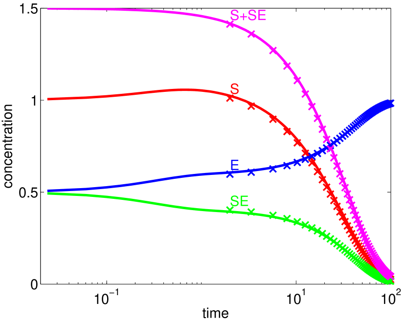
Figure 1: Comparison of numerical solutions obtained with the full Michaelis-Menten model (continuous lines) and with the reduced model (crosses). The variables $S$, $E$ and $SE$ are fast and slaved (in the reduced model, their values are obtained as solutions of algebraic equations) and the approximate conservation law $S+SE$ is slow. The initial values are such that $E$ and $S$ have concentrations of the same order of magnitude; this is not compatible with the quasi-steady state (QSS) approximation [52, 46] of the MM mechanism but is compatible with the quasi-equilibrium (QE) approximation that has been used here. As discussed in [34, 43, 46] the QE and QSS approximations correspond to scalings obtained from different tropical equilibration solutions (the total equilibration for QE and a partial equilibration solution for QSS).

4.4 Approximate Conservation Laws as Slow Variables

We have seen in the previous section that the approximate linear conservation laws of the Michaelis-Menten model are either exact conservation laws or slow variables. In this section we show that this property is true in general for any polynomial CRN model of type (1) and for all linear, monomial, or polynomial approximate conservation laws.

4.4.1 Linear Approximate Conservation Laws as Slow Variables

Linear approximate conservation laws correspond to “pools” of species that are conserved by fast cycling reactions. The exact and approximate linear conservation laws usually correspond to the total number of copies of a certain type of molecule in the pool. For instance, in Example 2, there is an exact and an approximate linear conservation law corresponding to the total numbers of enzyme and substrate molecules, respectively. The fast part of the dynamics ends with the equilibration of all species in the fast pool. This state is named quasi-equilibrium (QE) [24].

Let us consider an approximate linear conservation law

$$\phi(\boldsymbol{x})=\sum_{i=1}^{n}c_{i}x_{i},\quad\mathrm{where}\ c_{i}\in\mathbb{N},$$

which is conserved by the truncated ODE system (16). Note that in the linear combination defining $\phi(\boldsymbol{x})$ we also admit that some of the coefficients $c_{i}$ are zero. Let $I=\{i\mid c_{i}\neq 0\}$ denote the set of indices of species involved in the fast pool quantity. Furthermore, in most applications the $c_{i}$ are small positive integers and we will assume that $c_{i}={O}(1)$. Using the Definitions 3 and 5 we obtain the following result.

Theorem 18.

If $\phi(\boldsymbol{x})$ is a simple linear approximate conservation law, then the variable $q=\phi(\boldsymbol{x})$ is either constant or slower than all the variables $\{x_{i}\mid i\in I\}$ of the system (1). Furthermore, if the timescales of all $x_{i}$ with $i\in I$ have the same order, then the concentrations of these variables have the same orders.

Before we start with the proof of the theorem, we show the following lemma.

Lemma 19.

Let

$$\phi(\boldsymbol{x})=\sum_{i=1}^{n}c_{i}x_{i}$$

be a simple linear approximate conservation law and let $I$ be defined as above. Then all the polynomials $f_{i}^{(1)}(\boldsymbol{k},\boldsymbol{x})$ in the truncated system (16) have the same order in $\delta$, i.e. $od_{i}+b_{i}=od_{i^{\prime}}+b_{i^{\prime}}$ for all $i,\,i^{\prime}\in I$. If furthermore, the timescales of the variables $x_{i}$ have the same order in $\delta$ for all $i\in I$, i.e. $b_{i}=b_{i^{\prime}}$ for all $i,\,i^{\prime}\in I$, then the concentrations $x_{i}$ have also the same order in $\delta$, i.e. $d_{i}=d_{i^{\prime}}$ for all $i,\,i^{\prime}\in I$.

Proof of Lemma 19.

In the variables $\boldsymbol{x}$ the truncated system reads as (see (16))

$$\dot{x}_{i}=\delta^{od_{i}}\dot{y}_{i}=f_{i}^{(1)}(\boldsymbol{k},\boldsymbol{x}),\quad\mathrm{where}\ f_{i}^{(1)}(\boldsymbol{k},\boldsymbol{x})=\delta^{od_{i}+b_{i}+o\mu}\bar{f}_{i}^{(1)}(\boldsymbol{\bar{k}},\boldsymbol{y}).$$

Since $\phi(\boldsymbol{x})$ is conserved by system (16), one has

$$\sum_{i=1}^{r}c_{i}f_{i}^{(1)}(\boldsymbol{k},\boldsymbol{x})=0$$

for all $\boldsymbol{k}$, $\boldsymbol{x}$. This can only be satisfied if for all $i\in I$ there is at least one $j\in I$ such that $f_{i}^{(1)}(\boldsymbol{k},\boldsymbol{x})$ and $f_{j}^{(1)}(\boldsymbol{k},\boldsymbol{x})$ have a common monomial. Since $q$ is simple, then for all $i,\,j\in I$ with $i\neq j$ either $f_{i}^{(1)}(\boldsymbol{k},\boldsymbol{x})$ and $f_{j}^{(1)}(\boldsymbol{k},\boldsymbol{x})$ share a monomial or there is finite sequence $i=i_{0},\,i_{1},\,\ldots,\,i_{k}=j$ such that $f_{i_{l}}^{(1)}(\boldsymbol{k},\boldsymbol{x})$ and $f_{i_{l+1}}^{(1)}(\boldsymbol{k},\boldsymbol{x})$ share a monomial for $0\leq l\leq k$. Since by the definition of the truncated system all the monomials in $f_{i}^{(1)}(\boldsymbol{k},\boldsymbol{x})$ have the same order, it follows that all the polynomials $f_{i}^{(1)}(\boldsymbol{k},\boldsymbol{x})$ for some $i\in I$ have the same order $\nu=od_{i}+b_{i}+o\mu$. The timescale order $\mu_{i}$ of $x_{i}$ is the order of

$$\frac{\dot{x}_{i}}{x_{i}}=\frac{f_{i}^{(1)}(\boldsymbol{k},\boldsymbol{x})}{x_{i}},$$

namely $\mu_{i}=\nu-od_{i}=b_{i}+o\mu$. Thus, if all $b_{i}$ are equal, then all $d_{i}$ are equal, for $i\in I$. ∎

Proof of Theorem 18 .

From the definition of $q$ it follows that

$$\dot{q}=\sum_{i\in I}c_{i}\dot{x}_{i}.$$

Since $q$ is conserved by the truncated system (16), we have that

$$\sum_{i=1}^{n}c_{i}\delta^{b_{i}+od_{i}+o\mu}\bar{f}_{i}^{(1)}(\boldsymbol{\bar{k}},\boldsymbol{y})=0$$ (32)

for all $\boldsymbol{\bar{k}}$, $\boldsymbol{y}$, $\delta$ and so

$$\dot{q}=\sum_{i=1}^{n}c_{i}\delta^{b_{i}+od_{i}+o\mu}\left(\bar{f}_{i}^{(1)}(\boldsymbol{\bar{k}},\boldsymbol{y})+\delta^{b^{\prime}_{i}}\bar{f}_{i}^{(2)}(\boldsymbol{\bar{k}},\boldsymbol{y},\delta)\right)=\sum_{i=1}^{n}c_{i}\delta^{b_{i}+b^{\prime}_{i}+od_{i}+o\mu}\bar{f}_{i}^{(2)}(\boldsymbol{\bar{k}},\boldsymbol{y},\delta).$$

Thus $\dot{q}=0$ if $f_{i}^{(2)}(\boldsymbol{\bar{k}},\boldsymbol{y},\delta)$ vanishes identically. In this case the approximate conservation law is also an exact one. If this is not the case, we can define $\mu_{q}$ as the order of the timescale of $q$, i.e. the order of $\frac{\dot{q}}{q}$. The order of $q$ is $\min\{od_{i}\mid i\in I\}$ and so

$$\mu_{q}=\min\{b_{i}+b_{i}^{\prime}+od_{i}+o\mu\mid i\in I\}-\min\{od_{i}\mid i\in I\}.$$

We prove now that $q$ is slower than all $x_{i}$ with $i\in I$, that is, we need to check that $b_{i}+o\mu<\mu_{q}$ for all $i\in I$. These conditions are equivalent to

$$b_{i}<\min\{b_{j}+b_{j}^{\prime}+od_{j}\mid j\in I\}-\min\{od_{j}\mid j\in I\}\quad\mathrm{for}\ \mathrm{all}\ i\in I.$$

According to the Lemma 19, $b_{i}=\nu-o\mu-od_{i}$ for all $i\in I$. Obviously, it is enough to prove that

$$\nu-o\mu-\min\{od_{j}\mid j\in I\}<\min\{b_{j}+b_{j}^{\prime}+od_{j}\mid j\in I\}-\min\{od_{j}\mid j\in I\},$$

which leads us to the inequation $\nu-o\mu<\min\{b_{j}+b_{j}^{\prime}+od_{j}\mid j\in I\}$. Since $\nu=b_{j}+od_{j}+o\mu$ and $b_{j}^{\prime}>0$ for all $j\in I$, all the above inequalities are satisfied.

The second part of the Theorem follows from the Lemma 19. ∎

Theorem 18 suggests that there is a link between timescales and concentrations of species contributing to a linear approximate conservation law. This link can be made more precise by using the vectors $\boldsymbol{x}_{k}$ introduced in Section 4.1, which group variables with the same timescale orders $\mu_{k}$ for $1\leq k\leq m$. We have the following structure theorem for approximate linear conservation laws.

Theorem 20.

If $\phi(\boldsymbol{x}_{1},\ldots,\boldsymbol{x}_{l})$ is a simple linear approximate conservation law depending on variables having timescale orders smaller than or equal to $\mu_{l}$, then

$$\phi(\boldsymbol{x}_{1},\ldots,\boldsymbol{x}_{l})=\sum_{k=1}^{l}\delta^{d_{q}+\mu_{l}-\mu_{k}}\langle\boldsymbol{c}_{k},\boldsymbol{z}_{k}\rangle,$$ (33)

where $\mu_{1}<\mu_{2}<\ldots<\mu_{l}$, $\boldsymbol{c}_{k}\in\mathbb{R}^{n_{k}}$ and $d_{q}$ is the order of the variable $q=\phi(\boldsymbol{x}_{1},\ldots,\boldsymbol{x}_{l})$. Thus,

$$\phi(\boldsymbol{x}_{1},\ldots,\boldsymbol{x}_{l})=\phi^{(1)}(\boldsymbol{x}_{l})+\phi^{(2)}(\boldsymbol{x}_{1},\ldots,\boldsymbol{x}_{l-1}),$$

where

$$\phi^{(1)}(\boldsymbol{x}_{l})=\delta^{d_{q}}\langle\boldsymbol{c}_{l},\boldsymbol{z}_{l}\rangle\quad\mathrm{and}\quad\phi^{(2)}(\boldsymbol{x}_{1},\ldots,\boldsymbol{x}_{l-1})={o}(\delta^{d_{q}}).$$

$\phi^{(1)}(\boldsymbol{x}_{l})$ contains the dominant lowest order terms of $\phi$. In other words, variables of the same timescale orders contribute to terms of the same order in the conservation law; the dominant terms in the conservation law depend only on the slowest variables $\boldsymbol{x}_{l}$.

Proof.

From Equation (32) it follows that

$$\mu_{i}+od_{i}=\mu_{l}+d_{q}$$ (34)

for all $i$ with $c_{i}\neq 0$, where $d_{q}=\min\left\{od_{i}\mid c_{i}\neq 0\right\}$. From regrouping the coefficients $c_{i}$ into vectors $\boldsymbol{c}_{k}$ corresponding to variables of the same timescales, we obtain

$$\phi=\sum_{k=1}^{l}\langle\boldsymbol{c}_{k},\boldsymbol{x}_{k}\rangle=\sum_{k=1}^{l}\delta^{od_{k}}\langle\boldsymbol{c}_{k},\boldsymbol{z}_{k}\rangle.$$ (35)

Finally, Equation (33) follows from (35) and (34). ∎

Remark 21.

A set of independent simple approximate conservation laws can be obtained from the truncated stoichiometric matrix $\boldsymbol{S}^{(1)}$ by using algorithms for the computation of a basis of simple vectors of the left kernel of a given integer coefficient matrix, i.e. vectors that can not be decomposed as a sum of two non-zero kernel vectors having more zero elements [51].

Example 22.

Consider the chemical reaction network

If the dynamics of this reaction network is of mass-action form, then it is given by the system of ODEs

$$\dot{x}_{1} = k_{2}x_{2}-k_{1}x_{1},$$

$$\dot{x}_{2} = k_{1}x_{1}-(k_{2}+k_{5})x_{2},$$

$$\dot{x}_{3} = k_{5}x_{2}+k_{4}x_{4}-k_{3}x_{3},$$

$$\dot{x}_{4} = k_{3}x_{3}-k_{4}x_{4}.$$

Let us assume that the parameter orders are $e_{1}=e_{2}=e_{3}=e_{4}=0$, $e_{5}=1$. Then the total tropical equilibrations are solutions of the system $d_{1}=d_{2}$, $\min\{d_{4},\,d_{2}+1\}=d_{3}$, $d_{3}=d_{4}$, that is $d_{1}=d_{2}\geq d_{4}-1$, $d_{3}=d_{4}$. Assuming that the concentration orders are given by the total tropical equilibration $d_{1}=d_{2}=-1$ and $d_{3}=d_{4}=-2$, we obtain the rescaled system

$$\dot{y}_{1} = \bar{k}_{2}y_{2}-\bar{k}_{1}y_{1},$$

$$\dot{y}_{2} = \bar{k}_{1}y_{1}-(\bar{k}_{2}+\epsilon\bar{k}_{5})y_{2},$$

$$\dot{y}_{3} = \epsilon^{2}\bar{k}_{5}y_{2}+\bar{k}_{4}y_{4}-\bar{k}_{3}y_{3},$$

$$\dot{y}_{4} = \bar{k}_{3}y_{3}-\bar{k}_{4}y_{4}.$$

Since $\epsilon$ occurs only with integer powers we have $\delta=\epsilon$. All species $x_{i}$ for $1\leq i\leq 4$ have the same timescale orders $\mu_{i}=0$ . The truncated system is

$$\dot{x}_{1} = k_{2}x_{2}-k_{1}x_{1},$$

$$\dot{x}_{2} = k_{1}x_{1}-k_{2}x_{2},$$

$$\dot{x}_{3} = k_{4}x_{4}-k_{3}x_{3},$$

$$\dot{x}_{4} = k_{3}x_{3}-k_{4}x_{4}$$

and the truncated stoichiometric matrix reads as

$$\boldsymbol{S}^{(1)}=\begin{pmatrix}-1&1&0&0\\ 1&-1&0&0\\ 0&0&-1&1\\ 0&0&1&-1\end{pmatrix}.$$

The truncated system has two simple conservation laws $\phi_{1}(\boldsymbol{x})=x_{1}+x_{2}$ and $\phi_{2}(\boldsymbol{x})=x_{3}+x_{4}$. These correspond to the species pools $q_{1}=x_{1}+x_{2}$ and $q_{2}=x_{3}+x_{4}$ that have timescale orders $\mu_{q_{1}}=1$ and $\mu_{q_{2}}=2$, respectively. Thus, $q_{1}$ and $q_{2}$ are slower than the species $x_{i}$ with $1\leq i\leq 4$. Note that the species concentrations in these pools have equal orders $d_{1}=d_{2}$ and $d_{3}=d_{4}$, consistent with the fact that in simple pools, species with the same timescales have the same concentration orders (see Lemma 19). This CRN has also the exact conservation law $\phi_{1}(\boldsymbol{x})+\phi_{2}(\boldsymbol{x})$, but this conservation law is not simple.

4.4.2 Monomial Approximate Conservation Laws as Slow Variables

We consider now a monomial conservation law

$$\phi(\boldsymbol{x})=\prod_{i=1}^{n}x_{i}^{m_{i}}$$

of the truncated system (16). As in Section 3.1, we admit that some of the exponents $m_{i}$ can be zero and define $I=\{i\mid 1\leq i\leq n,\,m_{i}\neq 0\}$. This means that the variables $x_{i}$ with $i\notin I$ do not appear in the conservation law.

Theorem 23.

If $\phi(\boldsymbol{x})$ is a simple monomial approximate conservation law, then the variable $q=\phi(\boldsymbol{x})$ is slower than all the variables $\{x_{i}\mid i\in I\}$ of system (1). Furthermore, all $x_{i}$ with $i\in I$ have the same timescale orders.

Proof.

Let us note that

$$\dot{q}=q\sum_{i\in I}m_{i}\frac{\dot{x}_{i}}{x_{i}}.$$

Since $\phi(\boldsymbol{x})$ is conserved by the truncated system (16), we have that

$$\sum_{i\in I}\frac{m_{i}}{x_{i}}f_{i}^{(1)}(\boldsymbol{k},\boldsymbol{x})=0,$$ (36)

for all $\boldsymbol{k}$, $\boldsymbol{x}$. As $\frac{f_{i}^{(1)}}{x_{i}}$ is a sum of rational monomials, (36) is only satisfied if for any $i\in I$ there is $j\in I$ such that $\frac{f_{i}^{(1)}}{x_{i}}$ and $\frac{f_{j}^{(1)}}{x_{j}}$ share a common monomial. Since $\phi(\boldsymbol{x})$ is simple, for all $i,\,j\in I$ either $\frac{f_{i}^{(1)}}{x_{i}}$ and $\frac{f_{j}^{(1)}}{x_{j}}$ share a common monomial or there is a sequence $i=i_{0},\,i_{1},\,\ldots,\,i_{k}=j$ such that $\frac{f_{i_{l}}^{(1)}}{x_{i_{l}}}$ and $\frac{f_{i_{l+1}}^{(1)}}{x_{i_{l+1}}}$ share a common monomial for $0\leq l\leq k-1$. Hence, the orders of $\frac{f_{i}^{(1)}(\boldsymbol{k},\boldsymbol{x})}{x_{i}}$ are the same for all $i\in I$. As the timescale orders of $x_{i}$ are the orders of $\frac{f_{i}^{(1)}(\boldsymbol{k},\boldsymbol{x})}{x_{i}}$, it follows that all $x_{i}$ with $i\in I$ have the same timescale orders.

In order to compute the timescale of $q$ we use

$$\frac{\dot{q}}{q}=\sum_{i\in I}m_{i}\frac{\dot{x}_{i}}{x_{i}}=\sum_{i\in I}m_{i}\delta^{b_{i}+o\mu}\frac{\bar{f}_{i}^{(1)}(\boldsymbol{\bar{k}},\boldsymbol{y})+\delta^{b^{\prime}_{i}}\bar{f}_{i}^{(2)}(\boldsymbol{\bar{k}},\boldsymbol{y},\delta)}{y_{i}}=\sum_{i\in I}m_{i}\delta^{b_{i}+b^{\prime}_{i}+o\mu}\frac{f_{i}^{(2)}(\boldsymbol{\bar{k}},\boldsymbol{y},\delta)}{y_{i}},$$

where the last equality follows from the fact that $\phi(\boldsymbol{x})$ is conserved by (16).

Let us denote by $\mu_{q}$ the order of the timescale of $q$, i.e. the order of $\frac{\dot{q}}{q}$. Assuming that all $m_{i}$ are small integers of order ${O}(\delta^{0})$, it follows that

$$\mu_{q}=\min\{b_{i}+b^{\prime}_{i}+o\mu\mid i\in I\}.$$

To prove that $q$ is slower than each of the variables $\{x_{i}\mid i\in I\}$, we need to show that for all $i\in I$ we have $\mu_{i}<\mu_{q}$. Thus we need to prove that $b_{i}<\min\{b_{j}+b^{\prime}_{j}\mid j\in I\}$ for all $i\in I$. As for all $i,\,j\in I$ we have $b_{i}=b_{j}$ and $b^{\prime}_{j}>0$, it follows that $b_{i}=\min\{b_{j}\mid j\in I\}<\min\{b_{j}+b^{\prime}_{j}\mid j\in I\}$ for all $i\in I$.

∎

Example 24.

The model

$$\dot{x}_{1}=x_{1}(x_{2}-x_{1})-\delta x_{1},\quad\dot{x}_{2}=x_{2}(x_{1}-x_{2})$$

is a mass action network described by

$$A_{1}+A_{2}\xrightarrow{1}2A_{2},\quad A_{1}+A_{2}\xrightarrow{1}\emptyset,\quad A_{2}+A_{2}\xrightarrow{1}\emptyset,\quad A_{1}\xrightarrow{\delta}\emptyset.$$

The truncated system

$$\dot{x}_{1}=x_{1}(x_{2}-x_{1}),\quad\dot{x}_{2}=x_{2}(x_{1}-x_{2})$$

has a continuous steady state variety $x_{1}=x_{2}$ and on which its Jacobian is singular. This model has $\phi(x_{1},x_{2})=x_{1}x_{2}$ as an approximate monomial simple conservation law. The intersection of the steady state variety with the set $\phi=c_{0}$ is the point $x_{1}=x_{2}=c_{0}/2$. The monomial conservation law is complete, since the $2\times 2$ minor of the Jacobian

$$\mathrm{det}(D_{\boldsymbol{x}}(x_{1}(x_{2}-x_{1}),x_{1}x_{2})^{T})=-2x_{1}^{2}$$

does not vanish for $x_{1}>0$. Including $q=x_{1}x_{2}$ among the variables leads to the ODE system

$$\dot{x}_{1}=x_{1}(x_{2}-x_{1})-\delta x_{1},\quad\dot{x}_{2}=x_{2}(x_{1}-x_{2}),\quad\dot{q}=-\delta q.$$

We note that in agreement with the Theorem 23 $x_{1}$ and $x_{2}$ have the same timescale order and that $q$ is a slower variable.

4.4.3 Polynomial Approximate Conservation Laws as Slow Variables

Let

$$\phi(\boldsymbol{x})=\sum_{j=1}^{r}c_{j}\boldsymbol{x}^{\boldsymbol{m}_{j}}$$

be an approximate polynomial conservation law, that is conserved by system (16), where $c_{j}\in\mathbb{R}\setminus\{0\}$ and $\boldsymbol{m}_{j}=(m_{1j},\dots,m_{nj})\in\mathbb{N}^{n}$. Let $I=\{i\mid m_{ij}\neq 0\text{ for some $j$ with }1\leq j\leq r\}$ so that $\phi(\boldsymbol{x})$ depends only on the variables $x_{i}$ with $i\in I$.

Theorem 25.

If $\phi(\boldsymbol{x})$ is a simple polynomial approximate conservation law, then the variable $q=\phi(\boldsymbol{x})$ is slower than all variables $x_{i}$ with $i\in I$ of system (1). Furthermore, if the timescales of the variables $x_{i}$ have the same order in $\delta$, i.e. $b_{i}=b_{i^{\prime}}$ for all $i,\,i^{\prime}\in I$, then the monomials in $\phi(\boldsymbol{x})$ have also the same order in $\delta$, i.e. $\langle\boldsymbol{d},\boldsymbol{m}_{j}\rangle=\langle\boldsymbol{d},\boldsymbol{m}_{j^{\prime}}\rangle$ for all $1\leq j,\,j^{\prime}\leq r$ such that $m_{i,j}\neq 0$ and $m_{i^{\prime},j^{\prime}}\neq 0$ for some $i,\,i^{\prime}\in I$.

Proof.

We note that

$$\dot{q}=\sum_{j=1}^{r}c_{j}x^{\boldsymbol{m}_{j}}(\sum_{i=1}^{r}m_{ij}\frac{\dot{x}_{i}}{x_{i}})=\sum_{i=1}^{n}\frac{\dot{x}_{i}}{x_{i}}(\sum_{m_{i,j}\neq 0}m_{ij}c_{j}\boldsymbol{x}^{\boldsymbol{m}_{j}}).$$

Let us define the sums of rational monomials

$$E_{i,j}(\boldsymbol{k},\boldsymbol{x})=\frac{f_{i}^{(1)}(\boldsymbol{k},\boldsymbol{x})}{x_{i}}m_{ij}c_{j}\boldsymbol{x}^{\boldsymbol{m}_{j}}.$$

Then the expressions $E_{i,j}(\boldsymbol{k},\boldsymbol{x})$ have the orders

$$b_{i}+o\mu+o\langle\boldsymbol{d},\boldsymbol{m}_{j}\rangle.$$

As $\phi(\boldsymbol{x})$ is conserved by (16) it follows that

$$\sum_{1\leq i\leq n,\,1\leq j\leq r,\,m_{i,j}\neq 0}E_{i,j}(\boldsymbol{k},\boldsymbol{x})=0$$ (37)

for all $\boldsymbol{k}$, $\boldsymbol{x}$. This is only possible if for any pair $(i,j)$ with $m_{i,j}\neq 0$, there is a pair $(i^{\prime},j^{\prime})$ with $m_{i^{\prime},j^{\prime}}\neq 0$ such that $E_{i,j}$ and $E_{i^{\prime},j^{\prime}}$ share a common monomial. Since $\phi(\boldsymbol{x})$ is simple, for all pairs $(i,j)$ and $(i^{\prime},j^{\prime})$ with $m_{i,j}\neq 0$ and $m_{i^{\prime},j^{\prime}}\neq 0$, either $E_{i,j}$ and $E_{i^{\prime},j^{\prime}}$ share a common monomial or there is a sequence of pairs

$$(i,j)=(i_{0},j_{0}),\,(i_{1},j_{1}),\,\ldots,\,(i_{k},j_{k})=(i^{\prime},j^{\prime})$$

such that $E_{i_{l},j_{l}}$ and $E_{i_{l+1},j_{l+1}}$ share a common monomial for $0\leq l\leq k-1$. Thus, the expressions $E_{i,j}$ have the same order for all pairs $(i,j)$ with $m_{i,j}\neq 0$, i.e. we have that

$$b_{i}+o\mu+o\langle\boldsymbol{d},\boldsymbol{m}_{j}\rangle=b_{i^{\prime}}+o\mu+o\langle\boldsymbol{d},\boldsymbol{m}_{j^{\prime}}\rangle$$

for all pairs $(i,j)$ and $(i^{\prime},j^{\prime})$ with $m_{i,j}\neq 0$ and $m_{i^{\prime},j^{\prime}}\neq 0$. In particular, if all variables $x_{i}$ have the same timescale order $b_{i}$ for $i\in I$, it follows that the scalar products $\langle\boldsymbol{d},\boldsymbol{m}_{j}\rangle$ are equal for all $1\leq j<r$ with $m_{i,j}\neq 0$ for some $i\in I$. This proves the second part of the theorem.

As $q$ is conserved by system (16), it follows that

$$\dot{q}=\sum_{i,j,m_{i,j}\neq 0}\delta^{b_{i}+b^{\prime}_{i}+o\mu}\frac{\bar{f}_{i}^{(2)}(\boldsymbol{\bar{k}},\boldsymbol{y},\delta)}{y_{i}}m_{ij}c_{j}\delta^{o\langle\boldsymbol{d},\boldsymbol{m}_{j}\rangle}\boldsymbol{y}^{\boldsymbol{m}_{j}}.$$

The timescale order of $q$ is

$$\mu_{q}=\min\{b_{i}+b^{\prime}_{i}+o\mu+o\langle\boldsymbol{d},\boldsymbol{m}_{j}\rangle\mid m_{ij}\neq 0\}-\min\{o\langle\boldsymbol{d},\boldsymbol{m}_{j}\rangle\mid 1\leq j\leq r\}.$$

Let $i\in I$ and $j$ such that $m_{i,j}\neq 0$. Using

$$b_{i}+o\mu+o\langle\boldsymbol{d},\boldsymbol{m}_{j}\rangle=\min\{b_{i}+o\mu+o<\boldsymbol{d},\boldsymbol{m}_{j}\rangle\mid m_{i,j}\neq 0\}$$

and $b^{\prime}_{i}>0$, we obtain

$$b_{i}+o\mu=\min\{b_{i}+o\mu+o\langle\boldsymbol{d},\boldsymbol{m}_{j}\rangle\mid m_{i,j}\neq 0\}-o\langle\boldsymbol{d},\boldsymbol{m}_{j}\rangle<\mu_{q},$$

meaning that $q$ is slower than all $x_{i}$ with $i\in I$.

∎

As in the case of linear conservation laws, i.e. Theorem 20, we have a structure theorem for approximate polynomial conservation laws.

Theorem 26.

If $\phi(\boldsymbol{x}_{1},\ldots,\boldsymbol{x}_{l})$ is a simple polynomial approximate conservation law depending on variables having timescale orders smaller than or equal to $\mu_{l}$, then

$$\phi(\boldsymbol{x}_{1},\ldots,\boldsymbol{x}_{l})=\sum_{k=1}^{l}\delta^{d_{q}+\mu_{l}-\mu_{k}}\langle\boldsymbol{c}_{k},\boldsymbol{\varphi}(\boldsymbol{z}_{k})\rangle,$$ (38)

where $\mu_{1}<\mu_{2}<\ldots<\mu_{l}$, $\boldsymbol{c}_{k}\in\mathbb{R}^{n_{k}}$, $\boldsymbol{\varphi}(\boldsymbol{z}_{k})\in\mathbb{R}^{n_{k}}[\boldsymbol{z}_{k}]$ and $d_{q}$ is the order of the variable $q=\phi(\boldsymbol{x}_{1},\ldots,\boldsymbol{x}_{l})$. Thus,

$$\phi(\boldsymbol{x}_{1},\ldots,\boldsymbol{x}_{l})=\phi^{(1)}(\boldsymbol{x}_{l})+\phi^{(2)}(\boldsymbol{x}_{1},\ldots,\boldsymbol{x}_{l-1}),$$

where

$$\phi^{(1)}(\boldsymbol{x}_{l})=\delta^{d_{q}}\langle\boldsymbol{c}_{l},\boldsymbol{\varphi}_{l}(\boldsymbol{z}_{l})\rangle\quad\mathrm{and}\quad\phi^{(2)}(\boldsymbol{x}_{1},\ldots,\boldsymbol{x}_{l-1})={o}(\delta^{d_{q}}).$$

$\phi^{(1)}(\boldsymbol{x}_{l})$ contains the dominant lowest order terms of $\phi$. In other words, variables of the same timescale orders contribute to monomials of the same order in the conservation law; the dominant monomials in the conservation law correspond to the slowest variables.

Proof.

It follows from (37) that

$$\mu_{i}+o\langle\boldsymbol{d},\boldsymbol{m}_{j}\rangle=\mu_{l}+d_{q}$$ (39)

for all pairs $(i,j)$ with $c_{j}\neq 0$ and $m_{i,j}\neq 0$, where $d_{q}=\min\left\{o\langle\boldsymbol{d},\boldsymbol{m}_{j}\rangle\mid c_{j}\neq 0\right\}$. From (39) we obtain that the variables $x_{i}$, $x_{i^{\prime}}$ appearing in the same monomial $c_{j}\boldsymbol{x}^{\boldsymbol{m}_{j}}$ of $\phi$ must have the same timescale orders, i.e. we have $\mu_{i}=\mu_{i^{\prime}}$. By regrouping the coefficients $c_{i}$ into vectors $\boldsymbol{c}_{k}$ corresponding to variables of the same timescales and using again (39), we obtain (38). ∎

4.5 The Model Reduction Algorithms

To wrap up all the above developed concepts, we propose in this section several model reduction algorithms. These take into account approximate conservation laws and are applicable to CRN models with multiple timescales and polynomial rate functions. We consider two types of reductions:

1. Reduction at the slowest timescale.

2. Nested reductions at intermediate timescales.

In case (i) all the variables except the slowest one are eliminated during the reduction procedure. The reduced model is an ODE for the slowest variable. The elimination of fast variables proceeds hierarchically, the fastest variables being eliminated first.

In case (ii) all fast variables up to the $(l-1)$-th fastest one satisfy polynomial quasi-steady state equations and can be eliminated. The remaining variables satisfy a reduced system of ODEs. The reduced dynamics takes place on the normally hyperbolic invariant manifold that is close to the critical manifold defined by the quasi-steady state equations. Changing $l$ from $l=1$ to $l=m$ one obtains $m$ nested attractive normally hyperbolic invariant manifolds along which the reduced dynamics evolves at successively slower timescales. Of course (i) follows from (ii) with $l=m$.

For both types of reduction (i) and (ii) the elimination of the fast variables is possible only if the truncated system at the $k$-th timescale (defined by the vector fields ${\boldsymbol{\bar{f}}}_{1}^{(1)},\ldots,{\boldsymbol{\bar{f}}}_{k}^{(1)}$) has non-degenerate steady states (with $1\leq k\leq m$ in case (i) and $1\leq k\leq l$ in case (ii)). When there are approximate conservation laws which are conserved by the truncated system, the non-degeneracy condition is not fulfilled and the standard reduction algorithm proposed in [27] does not apply. Our solution to this problem is to add approximate conservation laws to the set of variables, eliminate some of the fast variables and obtain a modified system that has no approximate conservation laws and satisfies the hyperbolicity condition.

4.5.1 The Slowest Timescale Reduction

As in [27] we introduce the small parameters $\delta_{l-1}=\delta^{b_{l}-b_{l-1}}$, for $2\leq l\leq m$ and the vector $\boldsymbol{\bar{\delta}}=(\delta_{1},\ldots,\delta_{m-1})$. Let us change the time variable to $\tau^{\prime}=\tau\delta_{1}\delta_{2}\ldots\delta_{m-1}$, the slowest timescale of the model. Then system (17) becomes

$$\delta_{1}\delta_{2}\ldots\delta_{m-1}\boldsymbol{z}^{\prime}_{1} = {\boldsymbol{\bar{f}}}^{(1)}_{1}(\boldsymbol{\bar{k}},\boldsymbol{z})+{\boldsymbol{\bar{g}}}_{1}(\boldsymbol{\bar{k}},\boldsymbol{z},\boldsymbol{\bar{\delta}}),$$

$$\vdots$$

$$\delta_{m-1}\boldsymbol{z}^{\prime}_{m-1} = {\boldsymbol{\bar{f}}}^{(1)}_{m-1}(\boldsymbol{\bar{k}},\boldsymbol{z})+{\boldsymbol{\bar{g}}}_{m-1}(\boldsymbol{\bar{k}},\boldsymbol{z},\boldsymbol{\bar{\delta}}),$$

$$\boldsymbol{z}^{\prime}_{m} = {\boldsymbol{\bar{f}}}^{(1)}_{m}(\boldsymbol{\bar{k}},\boldsymbol{z})+{\boldsymbol{\bar{g}}}_{m}(\boldsymbol{\bar{k}},\boldsymbol{z},\boldsymbol{\bar{\delta}}),$$ (40)

where ${\boldsymbol{\bar{g}}}_{k}(\boldsymbol{\bar{k}},\boldsymbol{z},\boldsymbol{\bar{\delta}})=\delta^{b^{\prime}_{k}}{\boldsymbol{\bar{f}}}^{(2)}_{k}(\boldsymbol{\bar{k}},\boldsymbol{z},\boldsymbol{\bar{\delta}})$ satisfy ${\boldsymbol{\bar{g}}}_{k}(\boldsymbol{\bar{k}},\boldsymbol{z},0)=0$ for $1\leq k\leq m$. We assume that the functions ${\boldsymbol{\bar{g}}}_{k}$ are smooth in all their arguments. The smoothness in $\boldsymbol{\bar{\delta}}$ can be tested algorithmically with methods introduced in [27].

By setting $\boldsymbol{\bar{\delta}}=\boldsymbol{0}$ in system (4.5.1) we obtain the slowest timescale reduced system

$$0 = {\boldsymbol{\bar{f}}}^{(1)}_{1}(\boldsymbol{\bar{k}},\boldsymbol{z}),$$

$$\vdots$$

$$0 = {\boldsymbol{\bar{f}}}^{(1)}_{m-1}(\boldsymbol{\bar{k}},\boldsymbol{z}),$$

$$\boldsymbol{z}^{\prime}_{m} = {\boldsymbol{\bar{f}}}^{(1)}_{m}(\boldsymbol{\bar{k}},\boldsymbol{z}).$$ (41)

For $\boldsymbol{k}\in\mathbb{R}_{>0}^{r}$ and $\boldsymbol{z}_{m}\in\mathbb{R}_{>0}^{n_{m}}$ a state $(\boldsymbol{z}_{1},\ldots,\boldsymbol{z}_{m-1})$ satisfying the system of equations

$${\boldsymbol{\bar{f}}}_{1}^{(1)}(\boldsymbol{\bar{k}},\boldsymbol{z}_{1},\ldots,\boldsymbol{z}_{m-1},\boldsymbol{z}_{m})=0,\,\ldots,\,{\boldsymbol{\bar{f}}}_{m-1}^{(1)}(\boldsymbol{\bar{k}},\boldsymbol{z}_{1},\ldots,\boldsymbol{z}_{m-1},\boldsymbol{z}_{m})=0$$ (42)

is called a quasi-steady state. System (42) is called the quasi-steady state condition.

Assume that system (42) can be solved for $(\boldsymbol{z}_{1},\ldots,\boldsymbol{z}_{m-1})$ in the following hierarchical way. First, there is a differentiable function ${\boldsymbol{\tilde{f}}}_{1}(\boldsymbol{\bar{k}},\boldsymbol{z}_{2},\ldots,\boldsymbol{z}_{m})$ such that

$${\boldsymbol{\bar{f}}}_{1}^{(1)}(\boldsymbol{\bar{k}},{\boldsymbol{\tilde{f}}}_{1}(\boldsymbol{\bar{k}},\boldsymbol{z}_{2},\ldots,\boldsymbol{z}_{m}),\boldsymbol{z}_{2},\ldots,\boldsymbol{z}_{m})=0.$$

Next, consider that there is a differentiable function ${\boldsymbol{\tilde{f}}}_{2}(\boldsymbol{\bar{k}},\boldsymbol{z}_{3},\ldots,\boldsymbol{z}_{m})$ such that

$${\boldsymbol{\bar{f}}}_{2}^{(1)}(\boldsymbol{\bar{k}},{\boldsymbol{\tilde{f}}}_{1}(\boldsymbol{\bar{k}},{\boldsymbol{\tilde{f}}}_{2}(\boldsymbol{\bar{k}},\boldsymbol{z}_{3},\ldots,\boldsymbol{z}_{m}),\ldots,\boldsymbol{z}_{m}),{\boldsymbol{\tilde{f}}}_{2}(\boldsymbol{\bar{k}},\boldsymbol{z}_{3},\ldots,\boldsymbol{z}_{m}),\ldots,\boldsymbol{z}_{m})=0.$$

Assuming that the procedure can go on, consider finally that there is a function ${\boldsymbol{\tilde{f}}}_{m-1}(\boldsymbol{\bar{k}},\boldsymbol{z}_{m})$ such that

$${\boldsymbol{\bar{f}}}_{m-1}^{(1)}(\boldsymbol{\bar{k}},\boldsymbol{z}_{1},\boldsymbol{z}_{2},\ldots,\boldsymbol{z}_{m-1},\boldsymbol{z}_{m})=0,$$

where $\boldsymbol{z}_{1}$, $\boldsymbol{z}_{2}$, $\ldots$, $\boldsymbol{z}_{m-1}$ are recursively replaced by ${\boldsymbol{\tilde{f}}}_{1}(\boldsymbol{\bar{k}},\boldsymbol{z}_{2},\ldots,\boldsymbol{z}_{m})$, ${\boldsymbol{\tilde{f}}}_{2}(\boldsymbol{\bar{k}},\boldsymbol{z}_{3},\ldots,\boldsymbol{z}_{m})$, $\ldots$, ${\boldsymbol{\tilde{f}}}_{m-1}(\boldsymbol{\bar{k}},\boldsymbol{z}_{m})$, respectively.

Consider the reduced system

$$\boldsymbol{z}^{\prime}_{m}=\boldsymbol{f}^{*}_{m}(\boldsymbol{\bar{k}},\boldsymbol{z}_{m}),$$ (43)

where $\boldsymbol{f}^{*}_{m}(\boldsymbol{\bar{k}},\boldsymbol{z}_{m})$ is obtained from ${\boldsymbol{\bar{f}}}_{m}^{(1)}(\boldsymbol{\bar{k}},\boldsymbol{z}_{1},\ldots,\boldsymbol{z}_{m})$ by substituting $\boldsymbol{z}_{1}$, $\boldsymbol{z}_{2}$, $\ldots$, $\boldsymbol{z}_{m-1}$ as above.

Solutions of system (4.5.1) in the limit $\boldsymbol{\bar{\delta}}\to 0$ were studied by Tikhonov [56], Hoppensteadt [25] and O’Malley [37]. They showed that under appropriate conditions (roughly speaking the non-degeneracy and hyperbolicity of the quasi-steady states $\boldsymbol{z}_{k-1}={\boldsymbol{\tilde{f}}}_{k-1}(\boldsymbol{\bar{k}},\boldsymbol{z}_{k},\ldots,\boldsymbol{z}_{m})$ for $2\leq k\leq m$, see Section 4.5.3), the solutions of the system (4.5.1) with initial conditions $\boldsymbol{z}_{i}(0)=g_{i}(\delta)$, where the $g_{i}(\delta)$ are differentiable functions, converge for $\boldsymbol{\bar{\delta}}\to 0$ to the solutions of the system (43) with initial conditions $\boldsymbol{z}_{m}(0)=g_{m}(0)$. By this reduction, called quasi-steady state approximation, all variables faster than the slowest one are eliminated and the reduced model describes the dynamics at the slowest timescale. This type of reduction is the most popular one in applications, for instance in physical chemistry (where it is known as the Semenov-Bodenstein quasi-steady state approximation [5, 53]) and in computational systems biology [41].

4.5.2 Nested Intermediate Timescale Reductions

This type of reduction was proposed by Cardin and Teixera [8] and algorithmically formalized by Kruff et al. in [27]. We call it nested, since the reduced dynamics at intermediate timescales are embedded in normally hyperbolic invariant manifolds that form a nested family (manifolds of slower variables are included in manifolds of faster variables). In [8] both manifolds were considered, the stable and unstable one. As in [27] we only consider here the stable case. The stable normally hyperbolic invariant manifolds attract and sequentially confine the dynamics of the system, with rates from fastest to slowest, and are used to obtain reductions valid at intermediate timescales.

We provide here the formal description of the reduction at an intermediate timescale of order $\delta^{b_{l}}=\delta^{b_{1}}\delta_{1}\delta_{2}\ldots\delta_{l-1}$, where $\delta_{l},\,1\leq l\leq m$ are defined as in the previous section.

Redefining the time into $\tau^{\prime}=\tau\delta^{b_{l}}$, where $1\leq l\leq m$, leads to the system

$$\delta_{1}\delta_{2}\ldots\delta_{l-1}\boldsymbol{z}^{\prime}_{1} = ({\boldsymbol{\bar{f}}}_{1}^{(1)}(\boldsymbol{\bar{k}},\boldsymbol{z})+{\boldsymbol{\bar{g}}}_{1}(\boldsymbol{\bar{k}},\boldsymbol{z},\boldsymbol{\bar{\delta}})),$$

$$\vdots$$

$$\delta_{l-1}\boldsymbol{z}^{\prime}_{l-1} = ({\boldsymbol{\bar{f}}}_{l-1}^{(1)}(\boldsymbol{\bar{k}},\boldsymbol{z})+{\boldsymbol{\bar{g}}}_{l-1}(\boldsymbol{\bar{k}},\boldsymbol{z},\boldsymbol{\bar{\delta}})),$$

$$\boldsymbol{z}^{\prime}_{l} = ({\boldsymbol{\bar{f}}}_{l}^{(1)}(\boldsymbol{\bar{k}},\boldsymbol{z})+{\boldsymbol{\bar{g}}}_{l}(\boldsymbol{\bar{k}},\boldsymbol{z},\boldsymbol{\bar{\delta}})),$$

$$\boldsymbol{z}^{\prime}_{l+1} = \delta_{l}({\boldsymbol{\bar{f}}}_{l+1}^{(1)}(\boldsymbol{\bar{k}},\boldsymbol{z})+{\boldsymbol{\bar{g}}}_{l+1}(\boldsymbol{\bar{k}},\boldsymbol{z},\boldsymbol{\bar{\delta}})),$$

$$\vdots$$

$$\boldsymbol{z}^{\prime}_{m} = \delta_{l}\delta_{l+1}\ldots\delta_{m-1}({\boldsymbol{\bar{f}}}_{m}^{(1)}(\boldsymbol{\bar{k}},\boldsymbol{z})+{\boldsymbol{\bar{g}}}_{m}(\boldsymbol{\bar{k}},\boldsymbol{z},\boldsymbol{\bar{\delta}})),$$ (44)

where $\boldsymbol{\bar{\delta}}=(\delta_{1},\ldots,\delta_{m-1})$ and ${\boldsymbol{\bar{g}}}_{k}(\boldsymbol{\bar{k}},\boldsymbol{z},\boldsymbol{\bar{\delta}})$ is a smooth functions with ${\boldsymbol{\bar{g}}}_{k}(\boldsymbol{\bar{k}},\boldsymbol{z},0)=0$ for all $1\leq k\leq m$. In the following we call the system

$$0 = {\boldsymbol{\bar{f}}}_{1}^{(1)}(\boldsymbol{\bar{k}},\boldsymbol{z}),$$

$$\vdots$$

$$0 = {\boldsymbol{\bar{f}}}_{l-1}^{(1)}(\boldsymbol{\bar{k}},\boldsymbol{z}),$$

$$\boldsymbol{z}^{\prime}_{l} = {\boldsymbol{\bar{f}}}_{l}^{(1)}(\boldsymbol{\bar{k}},\boldsymbol{z}),$$

$$\boldsymbol{z}^{\prime}_{l+1} = \delta_{l}({\boldsymbol{\bar{f}}}_{l+1}^{(1)}(\boldsymbol{\bar{k}},\boldsymbol{z})+{\boldsymbol{\bar{g}}}_{l+1}(\boldsymbol{\bar{k}},\boldsymbol{z},\boldsymbol{\bar{\delta}})),$$

$$\vdots$$

$$\boldsymbol{z}^{\prime}_{m} = \delta_{l}\delta_{l+1}\ldots\delta_{m-1}({\boldsymbol{\bar{f}}}_{m}^{(1)}(\boldsymbol{\bar{k}},\boldsymbol{z})+{\boldsymbol{\bar{g}}}_{m}(\boldsymbol{\bar{k}},\boldsymbol{z},\boldsymbol{\bar{\delta}})),$$ (45)

where $\boldsymbol{\bar{\delta}}=(0,\ldots,0,\delta_{l},\ldots,\delta_{m-1})$, which we obtained from (4.5.2) by setting $\delta_{1},\,\delta_{2},\,\ldots,\,\delta_{l-1}$ to zero, the reduced system at the $l$-th fastest time or slower. In this case as well, the system of equations ${\boldsymbol{\bar{f}}}_{1}^{(1)}(\boldsymbol{\bar{k}},\boldsymbol{z})=0,\,\ldots,\,{\boldsymbol{\bar{f}}}_{l-1}^{(1)}(\boldsymbol{\bar{k}},\boldsymbol{z})=0$ corresponds to the quasi-steady state condition. In [27] we have also defined the simpler reduced system obtained by setting $\delta_{1},\,\delta_{2}\,\ldots,\,\delta_{m-1}$ in (4.5.2) to zero, namely

$$0 = {\boldsymbol{\bar{f}}}_{1}^{(1)}(\boldsymbol{\bar{k}},\boldsymbol{z}),$$

$$\vdots$$

$$0 = {\boldsymbol{\bar{f}}}_{l-1}^{(1)}(\boldsymbol{\bar{k}},\boldsymbol{z}),$$

$$\boldsymbol{z}^{\prime}_{l} = {\boldsymbol{\bar{f}}}_{l}^{(1)}(\boldsymbol{\bar{k}},\boldsymbol{z}),$$

$$\boldsymbol{z}^{\prime}_{l+1} = 0,$$

$$\vdots$$

$$\boldsymbol{z}^{\prime}_{m} = 0.$$ (46)

This reduced model emphasizes three groups of variables: slaved variables $\boldsymbol{z}_{1},\ldots,\boldsymbol{z}_{l-1}$, which are faster than $\delta^{b_{l}}$, driving variables $\boldsymbol{z}_{l}$, which have timescale $\delta^{b_{l}}$, and quenched variables $\boldsymbol{z}_{l+1},\,\ldots,\,\boldsymbol{z}_{m}$, which are slower than $\delta^{b_{l}}$. If regularity and hyperbolicity conditions are satisfied (see [8] and Section 4.5.3), then the solutions of system (4.5.2) converge to the solutions of system (4.5.2) when $\epsilon_{k}\to 0$ for $1\leq k\leq l-1$ (see the Corollary of Theorem A in [8]).

The limit $(\delta_{l},\ldots,\delta_{m-1})\to 0$ leading from system (4.5.2) to system (4.5.2) can be treated in the simpler framework of regular perturbations. Using the same regularity and hyperbolicity conditions, one can show that there is a time $T>0$ such that the solutions of system (4.5.2) converge for $\boldsymbol{\bar{\delta}}\to 0$ uniformly on any close subinterval of $(0,T]$ to the solutions of system (4.5.2) (cf. Theorem 1 of [27]). This result implies that the reduction (4.5.2) is valid on a time interval $[t_{1}\delta^{-b_{l}},t_{2}\delta^{-b_{l}}]$ with $[t_{1},t_{2}]\subset(0,T]$. The reduction $\eqref{truncatedmultiscale}$ has a broader validity including times longer than $\delta^{-b_{l}}$.

4.5.3 Hyperbolically Attractive Chains and Quasi-steady State Conditions

The two types of reductions presented in the previous section are based on hierarchical elimination of fast variables, previously discussed in [27]. We revisit here this construction, using the concept of the Schur complement.

Let us define

$$\boldsymbol{Z}_{k}=\begin{pmatrix}\boldsymbol{z}_{1}\\ \vdots\\ \boldsymbol{z}_{k}\end{pmatrix}\quad\mathrm{and}\quad{\boldsymbol{\bar{F}}}_{k}^{(1)}(\boldsymbol{\bar{k}},\boldsymbol{z})=\begin{pmatrix}{\boldsymbol{\bar{f}}}^{(1)}_{1}(\boldsymbol{\bar{k}},\boldsymbol{z})\\ \vdots\\ {\boldsymbol{\bar{f}}}^{(1)}_{k}(\boldsymbol{\bar{k}},\boldsymbol{z})\end{pmatrix}.$$

For any $1\leq k\leq m$, the system of equations ${\boldsymbol{\bar{F}}}_{k}^{(1)}(\boldsymbol{\bar{k}},\boldsymbol{z})=0$ defines the $k$-th quasi-steady variety. The set of positive solutions $\boldsymbol{z}$ of ${\boldsymbol{\bar{F}}}_{k}^{(1)}(\boldsymbol{\bar{k}},\boldsymbol{z})=0$ is denoted by ${\mathcal{M}}_{k}$ and represents the intersection of the $k$-th quasi-steady state variety with the first orthant. For $1\leq l\leq m$ we call the chain $\mathbb{R}_{>0}^{n}={\mathcal{M}}_{0}\supseteq{\mathcal{M}}_{1}\supseteq\ldots\supseteq{\mathcal{M}}_{l}$ of nested quasi-steady state varieties lying in the first orthant an $l$-chain.

We solve the equations ${\boldsymbol{\bar{F}}}_{k}^{(1)}(\boldsymbol{\bar{k}},\boldsymbol{z})=0$ by successive elimination of variables, starting with $\boldsymbol{z}_{1}$ and ending with $\boldsymbol{z}_{k}$. During the elimination process, intermediary functions $\boldsymbol{f}_{k}^{*}(\boldsymbol{\bar{k}},\boldsymbol{z}_{k},$ $\ldots,\boldsymbol{z}_{m})$, ${\boldsymbol{\tilde{f}}}_{k}(\boldsymbol{\bar{k}},\boldsymbol{z}_{k+1},\ldots,\boldsymbol{z}_{m})$ and ${\boldsymbol{\tilde{F}}}_{k}(\boldsymbol{\bar{k}},\boldsymbol{z}_{k+1},\ldots,\boldsymbol{z}_{m})$ are defined recursively. More precisely, let

$$\boldsymbol{f}_{1}^{*}(\boldsymbol{\bar{k}},\boldsymbol{z}_{1},\ldots,\boldsymbol{z}_{m})={\boldsymbol{\bar{f}}}_{1}^{(1)}(\boldsymbol{\bar{k}},\boldsymbol{z}_{1},\ldots,\boldsymbol{z}_{m})$$

and let $\boldsymbol{z}_{1}={\boldsymbol{\tilde{f}}}_{1}(\boldsymbol{\bar{k}},\boldsymbol{z}_{2},\ldots,\boldsymbol{z}_{m})$ be the locally unique solution of $\boldsymbol{f}_{1}^{*}(\boldsymbol{\bar{k}},\boldsymbol{z}_{1},\ldots,\boldsymbol{z}_{m})=0$ and set

$${\boldsymbol{\tilde{F}}}_{1}(\boldsymbol{\bar{k}},\boldsymbol{z}_{2},\ldots,\boldsymbol{z}_{m})={\boldsymbol{\tilde{f}}}_{1}(\boldsymbol{\bar{k}},\boldsymbol{z}_{2},\ldots,\boldsymbol{z}_{m}).$$

Giving this initial data one continues then recursively for $2\leq k\leq m-1$ in the following way: Define

$$\boldsymbol{f}_{k}^{*}(\boldsymbol{\bar{k}},\boldsymbol{z}_{k},\ldots,\boldsymbol{z}_{m})={\boldsymbol{\bar{f}}}_{k}^{(1)}(\boldsymbol{\bar{k}},{\boldsymbol{\tilde{F}}}_{k-1}(\boldsymbol{\bar{k}},\boldsymbol{z}_{k},\ldots,\boldsymbol{z}_{m}),\boldsymbol{z}_{k},\ldots,\boldsymbol{z}_{m}),$$ (47)

determine the locally unique solution

$$\boldsymbol{z}_{k}={\boldsymbol{\tilde{f}}}_{k}(\boldsymbol{\bar{k}},\boldsymbol{z}_{k+1},\ldots,\boldsymbol{z}_{m})$$ (48)

of $\boldsymbol{f}_{k}^{*}(\boldsymbol{\bar{k}},\boldsymbol{z}_{k},\ldots,\boldsymbol{z}_{m})=0$ and then set

$${\boldsymbol{\tilde{F}}}_{k}(\boldsymbol{\bar{k}},\boldsymbol{z}_{k+1},\ldots,\boldsymbol{z}_{m})=\begin{pmatrix}{\boldsymbol{\tilde{F}}}_{k-1}(\boldsymbol{\bar{k}},{\boldsymbol{\tilde{f}}}_{k}(\boldsymbol{\bar{k}},\boldsymbol{z}_{k+1},\ldots,\boldsymbol{z}_{m}),\boldsymbol{z}_{k+1},\ldots,\boldsymbol{z}_{m})\\ {\boldsymbol{\tilde{f}}}_{k}(\boldsymbol{\bar{k}},\boldsymbol{z}_{k+1},\ldots,\boldsymbol{z}_{m})\end{pmatrix}.$$ (49)

From the recursion the following proposition follows immediately.

Proposition 27.

The vector $\boldsymbol{z}=({\boldsymbol{\tilde{F}}}_{k}(\boldsymbol{\bar{k}},\boldsymbol{z}_{k+1},\ldots,\boldsymbol{z}_{m}),\boldsymbol{z}_{k+1},\ldots,\boldsymbol{z}_{m})$ is a solution of ${\boldsymbol{\bar{F}}}_{k}^{(1)}(\boldsymbol{\bar{k}},\boldsymbol{z})=0$.

The existence of the implicit functions ${\boldsymbol{\tilde{f}}}_{k}$ and ${\boldsymbol{\tilde{F}}}_{k}$ needs the following non-degeneracy condition.

Condition 28.

The solution $\boldsymbol{z}_{k}$ of the equation $\boldsymbol{f}_{k}^{*}(\boldsymbol{\bar{k}},\boldsymbol{z}_{k},\ldots,\boldsymbol{z}_{m})=0$ is non-degenerate, i.e. $\mathrm{det}(D_{\boldsymbol{z}_{k}}\boldsymbol{f}_{k}^{*})\neq 0$.

This condition can be written more conveniently.

Theorem 29.

For $1\leq k\leq l$ the implicit functions ${\boldsymbol{\tilde{f}}}_{k}(\boldsymbol{\bar{k}},\boldsymbol{z}_{k+1},\ldots,\boldsymbol{z}_{m})$ and ${\boldsymbol{\tilde{F}}}_{k}(\boldsymbol{\bar{k}},\boldsymbol{z}_{k+1},$ $\ldots,\boldsymbol{z}_{m})$ exist and are differentiable, if and only if

$$\mathrm{det}(D_{\boldsymbol{Z}_{k}}{\boldsymbol{\bar{F}}}_{k}^{(1)})\neq 0\text{ for all }\boldsymbol{z}\in{\cal M}_{k}.$$ (50)

In order to prove Theorem50 we need the Schur complement, which occurs naturally during the Gaussian elimination of variables (see, for instance, [62]).

Definition 30.

Let $M=\begin{pmatrix}A&B\\ C&D\end{pmatrix}$ be a block matrix with $A$ invertible. The matrix $M/A=D-CA^{-1}B$ is called the Schur complement of the block $A$ of $M$.

The Schur complement can be obtained from the following successive computations:

• Solve $AX+BY=0$ for $X$.

• Substitute $X$ in $CX+DY$, which leads to $(M/A)Y$.

Moreover, the Schur complement has the follwoing two simple properties [62]:

$$\mathrm{det}(M) = \mathrm{det}(M/A)\,\mathrm{det}(A)\quad\quad\text{(Schur formula), }$$ (51)

$$\mathrm{rk}(M) = \mathrm{rk}(M/A)+\mathrm{rk}(A)\quad\quad\text{(Guttman rank additivity formula). }$$ (52)

Returning to our problem, we prove now the following lemma.

Lemma 31.

The matrix $D_{\boldsymbol{z}_{k+1}}\boldsymbol{f}_{k+1}^{*}$ is a Schur complement. More precisely, we have

$$D_{\boldsymbol{z}_{k+1}}\boldsymbol{f}_{k+1}^{*}=D_{\boldsymbol{Z}_{k+1}}{\boldsymbol{\bar{F}}}_{k+1}^{(1)}/D_{\boldsymbol{Z}_{k}}{\boldsymbol{\bar{F}}}_{k}^{(1)},$$ (53)

for all $1\leq k\leq m-1$ and $\boldsymbol{z}\in{\cal M}_{k}$ such that $D_{\boldsymbol{Z}_{k}}{\boldsymbol{\bar{F}}}_{k}^{(1)}$ is invertible.

Proof.

We differentiate (47) with respect to $\boldsymbol{z}_{k+1}$ and obtain

$$D_{\boldsymbol{z}_{k+1}}\boldsymbol{f}_{k+1}^{*}=(D_{\boldsymbol{Z}_{k}}{\boldsymbol{\bar{f}}}_{k+1}^{(1)})D_{\boldsymbol{z}_{k+1}}{\boldsymbol{\tilde{F}}}_{k}+D_{\boldsymbol{z}_{k+1}}{\boldsymbol{\bar{f}}}_{k+1}^{(1)}.$$

From Proposition 27 we have that

$${\boldsymbol{\bar{F}}}_{k}^{(1)}(\boldsymbol{\bar{k}},{\boldsymbol{\tilde{F}}}_{k}(\boldsymbol{\bar{k}},\boldsymbol{z}_{k+1},\ldots,\boldsymbol{z}_{m}),\boldsymbol{z}_{k+1},\ldots,\boldsymbol{z}_{m})=0.$$

Differentiating the last equation with respect to $\boldsymbol{z}_{k+1}$ we obtain

$$(D_{\boldsymbol{Z}_{k}}{\boldsymbol{\bar{F}}}_{k}^{(1)})D_{\boldsymbol{z}_{k+1}}{\boldsymbol{\tilde{F}}}_{k}+D_{\boldsymbol{z}_{k+1}}{\boldsymbol{\bar{F}}}_{k}^{(1)}=0$$

for $\boldsymbol{z}\in{\cal M}_{k}$. Finally, we get

$$D_{\boldsymbol{z}_{k+1}}\boldsymbol{f}_{k+1}^{*}=-(D_{\boldsymbol{Z}_{k}}{\boldsymbol{\bar{f}}}_{k+1}^{(1)})(D_{\boldsymbol{Z}_{k}}{\boldsymbol{\bar{F}}}_{k}^{(1)})^{-1}D_{\boldsymbol{z}_{k+1}}{\boldsymbol{\bar{F}}}_{k}^{(1)}+D_{\boldsymbol{z}_{k+1}}{\boldsymbol{\bar{f}}}_{k+1}^{(1)}=D_{\boldsymbol{Z}_{k+1}}{\boldsymbol{\bar{F}}}_{k+1}^{(1)}/D_{\boldsymbol{Z}_{k}}{\boldsymbol{\bar{F}}}_{k}^{(1)}.$$

∎

Now we can prove Theorem 29.

Proof of Theorem 29 .

Using Schur formula (51) and Lemma 31, we obtain that

$$\mathrm{det}(D_{\boldsymbol{z}_{k}}\boldsymbol{f}_{k}^{*})\,\mathrm{det}(D_{\boldsymbol{Z}_{k-1}}{\boldsymbol{\bar{F}}}_{k-1}^{(1)})=\mathrm{det}(D_{\boldsymbol{Z}_{k}}{\boldsymbol{\bar{F}}}_{k}^{(1)})$$

for $2\leq k\leq l$ and that

$$\mathrm{det}(D_{\boldsymbol{z}_{1}}\boldsymbol{f}_{1}^{*})=\mathrm{det}(D_{\boldsymbol{Z}_{1}}{\boldsymbol{\bar{F}}}_{1}^{(1)}).$$

This implies that $\mathrm{det}(D_{\boldsymbol{z}_{k}}\boldsymbol{f}_{k}^{*})\neq 0$ for $1\leq k\leq l$ is equivalent to $\mathrm{det}(D_{\boldsymbol{Z}_{k}}{\boldsymbol{\bar{F}}}_{k}^{(1)})\neq 0$ for $1\leq k\leq l$. ∎

As discussed in [27] and [37], the validity of the quasi-steady state approximation depends also on the following hyperbolicity condition:

Condition 32 (Hyperbolicity).

For all $1\leq k\leq m$ the solution $\boldsymbol{z}_{k}={\boldsymbol{\tilde{f}}}_{k}(\boldsymbol{\bar{k}},\boldsymbol{z}_{k+1},\ldots,\boldsymbol{z}_{m})$ is a hyperbolically stable steady state of the ODE

$$\boldsymbol{z}_{k}^{\prime}=\boldsymbol{f}^{*}_{k}(\boldsymbol{\bar{k}},\boldsymbol{z}_{k},\boldsymbol{z}_{k+1},\ldots,\boldsymbol{z}_{m}),$$

where $\boldsymbol{f}^{*}_{k}$ is defined as in the subsection 4.5.3. Here, by hyperbolically stable we mean that all eigenvalues of the Jacobian matrix at the steady state have strictly negative real parts. The validity of the nested reduction at the $l$-th fastest time or slower requires that Condition 32 is fulfilled for all $1\leq k\leq l$.

As discussed in [27], an important concept for the geometric theory of singular perturbations is the hyperbolically attractive chain.

Definition 33.

An $l$-chain of nested quasi-steady state varieties ${\mathcal{M}}_{0}\supseteq{\mathcal{M}}_{1}\supseteq\ldots\supseteq{\mathcal{M}}_{l}$ is called a hyperbolically attractive $l$-chain if for all $1\leq k\leq l$ all eigenvalues of $D_{\boldsymbol{z}_{k}}\boldsymbol{f}_{k}^{*}$ have strictly negative real parts for $\boldsymbol{z}\in{\mathcal{M}}_{k}$. In this case we write ${\mathcal{M}}_{0}\rhd{\mathcal{M}}_{1}\rhd\ldots\rhd{\mathcal{M}}_{l}$.

Summarizing, the nested reduction (4.5.2) is valid up to the $l$-th timescale if the $l$-chain ${\mathcal{M}}_{0}\rhd{\mathcal{M}}_{1}\rhd\ldots\rhd{\mathcal{M}}_{l}$ is hyperbolically attractive (see [8, 27]). The slowest timescale quasi-steady state reduction (43) is valid if the $m$-chain ${\mathcal{M}}_{0}\rhd{\mathcal{M}}_{1}\rhd\ldots\rhd{\mathcal{M}}_{m}$ is hyperbolically attractive.

From Lemma 31 we obtain the following proposition.

Proposition 34.

An $l$-chain is hyperbolically attractive if and only if $\mathrm{det}(D_{\boldsymbol{Z}_{k}}{\boldsymbol{\bar{F}}}_{k}^{(1)})\neq 0$ for all $1\leq k\leq l$, all eigenvalues of $D_{\boldsymbol{z}_{1}}{\boldsymbol{\bar{f}}}_{1}^{(1)}$ have negative real parts for all $\boldsymbol{z}\in{\cal M}_{1}$ and for all $2\leq k\leq l$ all eigenvalues of $D_{\boldsymbol{Z}_{k}}{\boldsymbol{\bar{F}}}_{k}^{(1)}/D_{\boldsymbol{Z}_{k-1}}{\boldsymbol{\bar{F}}}_{k-1}^{(1)}$ have negative real parts for all $\boldsymbol{z}\in{\cal M}_{k-1}$.

4.5.4 Approximate Conservation Laws and the Quasi-equilibrium Condition

Linear approximate conservation laws were already proposed as a tool for model reduction of CRNs when the so-called quasi-equilibrium (QE) condition [24, 41] is satisfied. At QE the direct and reverse rates of fast reversible reactions compensate each other and the net rates of change of reactants and products are negligible. Products or reactants of fast reactions are fast species. However, although concentrations of fast species are equilibrated, these variables can not be eliminated by using the quasi-steady state (QSS) equations. In the case of QE linear combinations of concentrations of fast species are conserved by the fast dynamics and the QSS equations have degenerate solutions indexed by the values of the conserved quantities [24, 41].

In this paper we show that the degeneracy of solutions of QSS equations is valid more generally, for any approximate conservation laws.

Let us denote by $\boldsymbol{x}_{l}$ and $\boldsymbol{X}_{l}=(\boldsymbol{x}_{1},\ldots,\boldsymbol{x}_{l})$ the set of variables of system (1) having time-scales of order $\mu_{l}$ and timescales equal to or faster than $\mu_{l}$, respectively. Furthermore, let $\boldsymbol{f}_{l}(\boldsymbol{k},\boldsymbol{x})$, $\boldsymbol{f}_{l}^{(1)}(\boldsymbol{k},\boldsymbol{x})$,

$$\boldsymbol{F}_{l}(\boldsymbol{k},\boldsymbol{x})=\begin{pmatrix}\boldsymbol{f}_{1}(\boldsymbol{k},\boldsymbol{x})\\ \vdots\\ \boldsymbol{f}_{l}(\boldsymbol{k},\boldsymbol{x})\end{pmatrix}\quad\mathrm{and}\quad\boldsymbol{F}_{l}^{(1)}(\boldsymbol{k},\boldsymbol{x})=\begin{pmatrix}\boldsymbol{f}_{1}^{(1)}(\boldsymbol{k},\boldsymbol{x})\\ \vdots\\ \boldsymbol{f}_{l}^{(1)}(\boldsymbol{k},\boldsymbol{x})\end{pmatrix}$$

be the full and truncated vector fields whose flows have timescales of order $\mu_{l}$, and timescales equal to or faster than $\mu_{l}$, respectively. In other words, these vector fields are the unscaled versions of the vector fields ${\boldsymbol{\bar{f}}}_{l}(\boldsymbol{\bar{k}},\boldsymbol{z})$, ${\boldsymbol{\bar{f}}}_{l}^{(1)}(\boldsymbol{\bar{k}},\boldsymbol{z})$, ${\boldsymbol{\bar{F}}}_{l}(\boldsymbol{\bar{k}},\boldsymbol{z})$ and ${\boldsymbol{\bar{F}}}_{l}^{(1)}(\boldsymbol{\bar{k}},\boldsymbol{z})$ introduced in Section 4.1.

Let $\phi_{l}(\boldsymbol{X}_{l})$ be a linear, monomial or polynomial approximate conservation law depending only on the variables $\boldsymbol{X}_{l}$ satisfying $D_{\boldsymbol{X}_{l}}\phi_{l}(\boldsymbol{X}_{l})\boldsymbol{F}_{l}^{(1)}=0$. This approximate conservation law can eventually also be exact, in which case it also satisfies $D_{\boldsymbol{X}_{l}}\phi_{l}(\boldsymbol{X}_{l})\boldsymbol{F}_{l}=0$. The existence of such an approximate conservation law implies the failure of Condition (50) in Theorem 29 as in the following proposition.

Proposition 35.

Let us assume that there is an approximate conservation law $\phi_{l}(\boldsymbol{X}_{l})$, where $1\leq l\leq m$. Then $\mathrm{det}(D_{\boldsymbol{Z}_{l}}{\boldsymbol{\bar{F}}}^{(1)}_{l})=0$ if $\boldsymbol{z}\in{\cal M}_{l}$.

Proof.

The definition of approximate conservation laws yields

$$D_{\boldsymbol{X}_{l}}\phi_{l}(\boldsymbol{X}_{l})\boldsymbol{F}^{(1)}_{l}(\boldsymbol{k},\boldsymbol{x})=0.$$ (54)

Since, up to the change of variables $\boldsymbol{\bar{k}}\leftarrow\boldsymbol{k}$ and $\boldsymbol{z}\leftarrow\boldsymbol{x}$, the polynomials $\boldsymbol{F}^{(1)}_{l}$ and ${\boldsymbol{\bar{F}}}^{(1)}_{l}$ are identical, we find

$$D_{\boldsymbol{Z}_{l}}\phi_{l}(\boldsymbol{Z}_{l}){\boldsymbol{\bar{F}}}^{(1)}_{l}(\boldsymbol{\bar{k}},\boldsymbol{z})=0.$$ (55)

Differentiating (55) we obtain

$$\frac{d^{2}\phi_{l}}{d{\boldsymbol{Z}_{l}}^{2}}{\boldsymbol{\bar{F}}}^{(1)}_{l}+\frac{d\phi_{l}}{d\boldsymbol{Z}_{l}}\frac{d{\boldsymbol{\bar{F}}}^{(1)}_{l}}{d\boldsymbol{Z}_{l}}=0,$$

where $\frac{d^{2}\phi_{l}}{d{\boldsymbol{Z}_{l}}^{2}}$ is the second derivative of $\phi_{l}$ with respect to $\boldsymbol{Z}_{l}$. If $\boldsymbol{z}\in{\cal M}_{l}$, then ${\boldsymbol{\bar{F}}}^{(1)}_{l}(\boldsymbol{\bar{k}},\boldsymbol{z})=0$ and therefore

$$\frac{d\phi_{l}}{d\boldsymbol{Z}_{l}}\frac{d{\boldsymbol{\bar{F}}}^{(1)}_{l}}{d\boldsymbol{Z}_{l}}=0.$$

Thus, the left kernel of the matrix $\frac{d{\boldsymbol{\bar{F}}}^{(1)}_{l}}{d\boldsymbol{Z}_{l}}$ contains the covector $\frac{d\phi_{l}}{d\boldsymbol{Z}_{l}}\neq 0$ and so $\mathrm{det}(D_{\boldsymbol{Z}_{l}}{\boldsymbol{\bar{F}}}^{(1)}_{l})=0$. ∎

In this case the quasi-steady state condition $\boldsymbol{F}_{l}^{(1)}(\boldsymbol{k},\boldsymbol{X}_{l},\boldsymbol{x}_{l+1},\ldots,\boldsymbol{x}_{m})=0$ can not be used to eliminate the fast variables $\boldsymbol{X}_{l}$. However, even in this case the CRN (1) can be transformed to an equivalent CRN that fulfils the nondegeneracy Condition (50) for $1\leq k\leq l$. The details of the transformation are presented below.

Let $\boldsymbol{\Phi}_{l}(\boldsymbol{X}_{l})=(\phi_{1l}(\boldsymbol{X}_{l}),\ldots,\phi_{s_{l}l}(\boldsymbol{X}_{l}))^{T}$ be a set of $s_{l}$ approximate conservation laws dependent on $\boldsymbol{X}_{l}$ and consider the equation

$$\boldsymbol{x}_{l}^{c}=\boldsymbol{\Phi}_{l}(\boldsymbol{X}_{l}).$$ (56)

Assuming that the conservation laws $\boldsymbol{\Phi}_{l}(\boldsymbol{X}_{l})$ are independent as functions of $\boldsymbol{x}_{l}$, namely that

$$\mathrm{rk}(D_{\boldsymbol{x}_{l}}\boldsymbol{\Phi}_{l}(\boldsymbol{X}_{l}))=s_{l},$$

we have, up to a relabelling of the components of $\boldsymbol{X}_{l}$, the splitting $\boldsymbol{X}_{l}=(\boldsymbol{X}_{l-1},\check{\boldsymbol{x}}_{l},\hat{\boldsymbol{x}}_{l})$, where $\boldsymbol{X}_{l-1}\in\mathbb{R}^{n_{1}+\ldots+n_{l-1}}$, $\check{\boldsymbol{x}}_{l}\in\mathbb{R}^{s_{l}}$, $\hat{\boldsymbol{x}}_{l}\in\mathbb{R}^{n_{l}-s_{l}}$ and $\mathrm{det}(D_{\check{\boldsymbol{x}}_{l}}\boldsymbol{\Phi}_{l})\neq 0$. Hence, (56) defines the implicit function $\check{\boldsymbol{x}}_{l}=\boldsymbol{\Psi}_{l}(\boldsymbol{X}_{l-1},\hat{\boldsymbol{x}}_{l},\boldsymbol{x}_{l}^{c})$, which allows to eliminate the variables $\check{\boldsymbol{x}}_{l}$.

The above splitting of $\boldsymbol{X}_{l}$ induces the splittings $\boldsymbol{F}_{l}=(\boldsymbol{F}_{l-1},{\boldsymbol{\check{f}}}_{l},{\boldsymbol{\hat{f}}}_{l})$ and $\boldsymbol{F}^{(i)}_{l}=(\boldsymbol{F}^{(i)}_{l-1},$ ${\boldsymbol{\check{f}}}^{(i)}_{l},{\boldsymbol{\hat{f}}}^{(i)}_{l})$ for $1\leq i\leq 2$. Let us define the functions

$$\boldsymbol{F}_{k}^{red}(\boldsymbol{k},{\boldsymbol{X}}_{l-1},\hat{\boldsymbol{x}}_{l},\boldsymbol{x}_{l}^{c},\boldsymbol{x}_{l+1},\boldsymbol{x}_{l+2},\ldots,\boldsymbol{x}_{m})=$$

$${\boldsymbol{\hat{F}}}_{k}(\boldsymbol{k},{\boldsymbol{X}}_{l-1},\boldsymbol{\Psi}_{l}(\boldsymbol{X}_{l-1},\hat{\boldsymbol{x}}_{l},\boldsymbol{x}_{l}^{c}),\hat{\boldsymbol{x}}_{l},\boldsymbol{x}_{l+1},\boldsymbol{x}_{l+2},\ldots,\boldsymbol{x}_{m}),$$ (57)

where ${\boldsymbol{\hat{F}}}_{k}=\boldsymbol{F}_{k}$ for $1\leq k\leq l-1$, and ${\boldsymbol{\hat{F}}}_{l}=(\boldsymbol{F}_{l-1},{\boldsymbol{\hat{f}}}_{l})$. The transformed model obtained from the substitution $\check{\boldsymbol{x}}_{l}=\boldsymbol{\Psi}_{l}(\boldsymbol{X}_{l-1},\hat{\boldsymbol{x}}_{l},\boldsymbol{x}_{l}^{c})$ is

$$\dot{\hat{\boldsymbol{X}}}_{l} = \boldsymbol{F}_{l}^{red}(\boldsymbol{k},{\boldsymbol{X}}_{l-1},\hat{\boldsymbol{x}}_{l},\boldsymbol{x}_{l}^{c},\boldsymbol{x}_{l+1},\boldsymbol{x}_{l+2},\ldots,\boldsymbol{x}_{m}),$$ (58)

$$\dot{\boldsymbol{x}}_{l}^{c} = ((D_{\boldsymbol{X}_{l}}\boldsymbol{\Phi}_{l})\boldsymbol{F}_{l}^{(2)})(\boldsymbol{k},{\boldsymbol{X}}_{l-1},\boldsymbol{\Psi}_{l}(\boldsymbol{X}_{l-1},\hat{\boldsymbol{x}}_{l},\boldsymbol{x}_{l}^{c}),\hat{\boldsymbol{x}}_{l},\boldsymbol{x}_{l+1},\boldsymbol{x}_{l+2},\ldots,\boldsymbol{x}_{m}),$$ (59)

$$\dot{\boldsymbol{x}}_{k} = \boldsymbol{f}_{k}(\boldsymbol{k},{\boldsymbol{X}}_{l-1},\boldsymbol{\Psi}_{l}(\boldsymbol{X}_{l-1},\hat{\boldsymbol{x}}_{l},\boldsymbol{x}_{l}^{c}),\hat{\boldsymbol{x}}_{l},\boldsymbol{x}_{l+1},\boldsymbol{x}_{l+2},\ldots,\boldsymbol{x}_{m}),\,k\in\{l+1,\ldots,m\}.$$ (60)

We have seen in Theorems 20 and 26) that $\boldsymbol{\Phi}_{l}=\boldsymbol{\Phi}_{l}^{(1)}(\boldsymbol{x}_{l})+{o}(\delta^{q_{f}})$, where $\boldsymbol{\Phi}_{l}^{(1)}(\boldsymbol{x}_{l})={O}(\delta^{q_{f}})$ is the lowest order (dominant) part of $\boldsymbol{\Phi}_{l}$. Furthermore, the dominant part $\boldsymbol{\Psi}^{(1)}_{l}$ of $\boldsymbol{\Psi}_{l}$ satisfies the equation

$$\boldsymbol{x}_{l}^{c}=\boldsymbol{\Phi}_{l}^{(1)}(\boldsymbol{\Psi}^{(1)}_{l}(\hat{\boldsymbol{x}}_{l},\boldsymbol{x}_{l}^{c}),\hat{\boldsymbol{x}_{l}}).$$ (61)

Thus, the truncated versions of the functions $\boldsymbol{F}_{k}^{red}$ are

$$\boldsymbol{F}_{k}^{red,1}(\boldsymbol{k},{\boldsymbol{X}}_{l-1},\hat{\boldsymbol{x}}_{l},\boldsymbol{x}_{l}^{c},\boldsymbol{x}_{l+1},\boldsymbol{x}_{l+2},\ldots,\boldsymbol{x}_{m})=$$

$${\boldsymbol{\hat{F}}}^{(1)}_{k}(\boldsymbol{k},{\boldsymbol{X}}_{l-1},\boldsymbol{\Psi}^{(1)}_{l}(\hat{\boldsymbol{x}}_{l},\boldsymbol{x}_{l}^{c}),\hat{\boldsymbol{x}}_{l},\boldsymbol{x}_{l+1},\boldsymbol{x}_{l+2},\ldots,\boldsymbol{x}_{m}),$$ (62)

where ${\boldsymbol{\hat{F}}}^{(1)}_{k}=\boldsymbol{F}^{(1)}_{k}$ for $1\leq k\leq l-1$, and ${\boldsymbol{\hat{F}}}^{(1)}_{l}=(\boldsymbol{F}^{(1)}_{l-1},{\boldsymbol{\hat{f}}}_{l})$.

We can state now the main result of this section. Let us assume that the following conditions are satisfied.

Condition 36.

 

1. For any $\boldsymbol{k}\in\mathbb{R}_{>0}^{r}$ there exist $\boldsymbol{x}\in\mathbb{R}_{>0}^{n}$ such that $\boldsymbol{F}^{(1)}_{l}(\boldsymbol{k},\boldsymbol{x})=0$. For all $\boldsymbol{x}\in\mathbb{R}_{>0}^{n}$ with $\boldsymbol{F}^{(1)}_{l}(\boldsymbol{k},\boldsymbol{x})=0$, we have $\mathrm{det}(D_{\boldsymbol{X}_{k}}{\boldsymbol{F}^{(1)}_{k}})\neq 0$ for all $1\leq k\leq l-1$ and $\mathrm{det}(D_{\boldsymbol{X}_{l}}{\boldsymbol{F}^{(1)}_{l}})=0$.

2. There is a set of $s_{l}$ simple approximate conservation laws

   $$\boldsymbol{\Phi}_{l}(\boldsymbol{X}_{l})=(\phi_{1l}(\boldsymbol{X}_{l}),\ldots,\phi_{s_{l}l}(\boldsymbol{X}_{l}))^{\mathsf{T}}$$

   depending only on $\boldsymbol{X}_{l}$ such that $(D_{\boldsymbol{X}_{l}}\boldsymbol{\Phi}_{l})\boldsymbol{F}^{(1)}_{l}=0$, , where $0<s_{l}\leq n_{l}$. For all $\boldsymbol{k}\in\mathbb{R}_{>0}^{r}$ and $\boldsymbol{x}\in\mathbb{R}_{>0}^{n}$ such that $\boldsymbol{F}^{(1)}_{l}(\boldsymbol{k},\boldsymbol{x})=0$ we have that

   $$\mathrm{rk}\left(D_{\boldsymbol{X}_{l}}\begin{pmatrix}\boldsymbol{\Phi}_{l}^{(1)}\\ {\boldsymbol{\hat{F}}}^{(1)}_{l}\end{pmatrix}\right)=n_{1}+\ldots+n_{l}.$$ (63)

3. The conservation laws $\boldsymbol{\Phi}_{l}(\boldsymbol{X}_{l})$ are independent as functions of $\boldsymbol{x}_{l}$, namely

   $$\mathrm{rk}(D_{\boldsymbol{x}_{l}}\boldsymbol{\Phi}_{l}(\boldsymbol{X}_{l}))=s_{l}.$$ (64)

Theorem 37.

If Condition 36 is fulfilled and

$$\boldsymbol{F}_{l}^{red,1}(\boldsymbol{k},{\boldsymbol{X}}_{l-1},\hat{\boldsymbol{x}}_{l},\boldsymbol{x}_{l}^{c},\boldsymbol{x}_{l+1},\boldsymbol{x}_{l+2},\ldots,\boldsymbol{x}_{m})=0,$$

then $\mathrm{det}(D_{\hat{\boldsymbol{X}}_{k}}\boldsymbol{F}_{k}^{(red,1)})\neq 0$ for all $1\leq k\leq l$, where $\hat{\boldsymbol{X}}_{k}={\boldsymbol{X}}_{k}$ for $1\leq k\leq l-1$ and $\hat{\boldsymbol{X}}_{l}=({\boldsymbol{X}}_{l-1},\hat{\boldsymbol{x}}_{l})$.

The proof of Theorem 37 uses the following lemma.

Lemma 38.

We have

$$D_{\hat{\boldsymbol{X}}_{l}}\boldsymbol{F}_{l}^{red,1}=D_{{\boldsymbol{X}}_{l}}\left.\begin{pmatrix}\boldsymbol{\Phi}_{l}^{(1)}\\ {\boldsymbol{\hat{F}}}^{(1)}_{l}\end{pmatrix}\right/D_{\check{\boldsymbol{x}}_{l}}\boldsymbol{\Phi}_{l}^{(1)}.$$

Proof.

Differentiating (61) with respect to $\hat{\boldsymbol{X}}_{l}$ we obtain

$$D_{\hat{\boldsymbol{X}}_{l}}\boldsymbol{\Phi}_{l}^{(1)}+D_{\check{\boldsymbol{x}}_{l}}\boldsymbol{\Phi}_{l}^{(1)}D_{\hat{\boldsymbol{X}}_{l}}\boldsymbol{\Psi}_{l}^{(1)}=0.$$

It follows from (62) that

$$D_{\hat{\boldsymbol{X}}_{l}}\boldsymbol{F}_{l}^{red,1}=D_{\hat{\boldsymbol{X}}_{l}}{\boldsymbol{\hat{F}}}^{(1)}_{l}+D_{\check{\boldsymbol{x}}_{l}}{\boldsymbol{\hat{F}}}^{(1)}_{l}D_{\hat{\boldsymbol{X}}_{l}}\boldsymbol{\Psi}_{l}^{(1)}=D_{\hat{\boldsymbol{X}}_{l}}{\boldsymbol{\hat{F}}}^{(1)}_{l}-D_{\check{\boldsymbol{x}}_{l}}{\boldsymbol{\hat{F}}}^{(1)}_{l}(D_{\check{\boldsymbol{x}}_{l}}\boldsymbol{\Phi}_{l}^{(1)})^{-1}D_{\hat{\boldsymbol{X}}_{l}}\boldsymbol{\Phi}_{l}^{(1)},$$

which completes the proof. ∎

Proof of Theorem 37.

We prove that $D_{\hat{\boldsymbol{X}}_{k}}\boldsymbol{F}_{k}^{red,1}$ is invertible for all $1\leq k\leq l$. Using the structure Theorems 20 and 26 we find that $D_{\boldsymbol{x}_{l}}\boldsymbol{\Phi}_{l}=D_{\boldsymbol{x}_{l}}\boldsymbol{\Phi}^{(1)}_{l}$. Thus, it follows from (64) that $\mathrm{rk}(D_{\boldsymbol{x}_{l}}\boldsymbol{\Phi}_{l}^{(1)})=s_{l}$. Using (63), the Guttman rank additivity formula (52) and Lemma 38, we find that

$$\mathrm{rk}\left(D_{\hat{\boldsymbol{X}}_{l}}\boldsymbol{F}_{l}^{red,1}\right)=n_{1}+n_{2}+\ldots+n_{l}-s_{l}$$

and so $D_{\hat{\boldsymbol{X}}_{l}}{\boldsymbol{\hat{F}}}_{l}^{red,1}$ is invertible. Since $\boldsymbol{\psi}_{l}^{(1)}$ does not depend on $\boldsymbol{X}_{k}$ for $1\leq k\leq l-1$, it follows that $D_{\hat{\boldsymbol{X}}_{k}}\boldsymbol{F}_{k}^{red,1}=D_{{\boldsymbol{X}}_{k}}\boldsymbol{F}_{k}^{(1)}$. Since $D_{{\boldsymbol{X}}_{k}}\boldsymbol{F}_{k}^{(1)}$ is invertible, the same is true for $D_{\hat{\boldsymbol{X}}_{k}}\boldsymbol{F}_{k}^{red,1}$.

∎

Remark 39.

Because conservation laws are used to eliminate the variables $\check{\boldsymbol{x}}_{l}$, the rank conditions (63) and (64) are satisfied if

$$\mathrm{det}\left(D_{\boldsymbol{X}_{l}}\begin{pmatrix}\boldsymbol{\Phi}_{l}^{(1)}\\ {\boldsymbol{\hat{F}}}^{(1)}_{l}\end{pmatrix}\right)\neq 0$$

and $\mathrm{det}(D_{\check{\boldsymbol{x}}_{l}}\boldsymbol{\Phi}_{l})\neq 0$, respectively.

Remark 40.

Theorem 37 allows to define $l$-chains in the case of a quasi-equilibrium. The set of positive solutions of the set of equations

$$\boldsymbol{F}_{k}^{red,1}(\boldsymbol{k},{\boldsymbol{X}}_{l-1},\hat{\boldsymbol{x}}_{l},\boldsymbol{x}_{l}^{c},\boldsymbol{x}_{l+1},\ldots,\boldsymbol{x}_{m})=0,$$

that is equivalent to

$${\boldsymbol{\hat{F}}}_{k}^{(1)}(\boldsymbol{k},{\boldsymbol{X}}_{l-1},{\boldsymbol{x}}_{l},\boldsymbol{x}_{l}^{c},\boldsymbol{x}_{l+1},\ldots,\boldsymbol{x}_{m})=0,\,\boldsymbol{\Phi}_{l}^{(1)}({\boldsymbol{x}}_{l})=\boldsymbol{x}_{l}^{c},$$

is denoted ${\cal M}_{k}^{QE}$ and represents the $k$-th quasi-equilibrium variety (intersected with the first orthant). These sets satisfy

$$\mathbb{R}_{>0}^{n}={\cal M}_{0}^{QE}\supset{\cal M}_{1}^{QE}\supset\ldots\supset{\cal M}_{l}^{QE}.$$

The concept of hyperbolically attractive $l-$chains is applicable to quasi-equilibrium varieties as well.

By the results of Section 4.4 the new variables $\boldsymbol{x}_{l}^{c}$ are slower than $\hat{\boldsymbol{X}}_{l}$ and by Theorem 37 the transformed model satisfies the non-degeneracy conditions $\mathrm{det}(D_{\hat{\boldsymbol{X}}_{k}}F_{k}^{(red,1)})\neq 0$ up to order $l$. If the approximate conservation laws are also exact, the new variables $\boldsymbol{x}_{l}^{c}$ are constant and stand for new parameters. Then, the new equations (59) are not added to the transformed ones (58) and (60). In this case as well, the transformed model (58) and (60) satisfies the non-degeneracy conditions up to order $l$.

4.5.5 Algorithmic Solution for Eliminating the Approximate Conservation Laws

The previous section allows us to define an algorithm which transforms the CRN (1) into an equivalent one that does not have approximate conservation laws and that can be further reduced using the method introduced in [27]. During this transformation, some old variables are substituted by new ones, representing approximate conservation laws that are not exact. Also, each exact conservation law leads to the creation of a new parameter and to the elimination of one variable together with the corresponding ODE.

Algorithm 1 transforms the CRN into another CRN that satisfies the condition $\mathrm{det}(D_{\boldsymbol{X}_{k}}$ $F_{k})\neq 0$ for all $1\leq k\leq l$ up to the $l$-th timescale. It further iterates the procedure for increasing $l$, computes a rescaled and truncated version of the CRN at each step by using the algorithm ScaleAndTruncate introduced in [27].

0:  A CRN given by a polynomial vector field $\boldsymbol{F}(\boldsymbol{k},\boldsymbol{x})$.

0:  A transformed CRN given by a modified polynomial vector field.

1:  ScaleAndTruncate.

2:  $l:=0$

3:  while $l<m$ do

4:     $l:=l+1$

5:     while $\mathrm{det}(D_{\boldsymbol{X}_{l}}F_{l}^{(1)})\neq 0$ do

6:        $l:=l+1$

7:     end while

8:     Find a complete set $\boldsymbol{\Phi}_{l}$ of independent conservation laws for $\boldsymbol{F}^{(1)}_{l}$ satisfying conditions (63) and (64).

9:      Compute the solution $\check{\boldsymbol{x}}_{l}=\boldsymbol{\psi}_{l}(\boldsymbol{X}_{l-1},\hat{\boldsymbol{x}}_{l},\boldsymbol{x}_{l}^{c})$ of the equation $\boldsymbol{x}_{l}^{c}=\boldsymbol{\Phi_{l}}(\boldsymbol{X}_{l-1},\hat{\boldsymbol{x}}_{l},\check{\boldsymbol{x}}_{l})$.

10:     for $i:=1$ to $s_{l}$ do

11:        if $\Phi_{il}$ is not exact then

12:           Replace the ODE satisfied by $\check{x}_{il}$ by $\dot{x}_{il}^{c}=(D_{\boldsymbol{x}}{\Phi}_{il})\boldsymbol{F}(\boldsymbol{k},\boldsymbol{x})$.

13:        else

14:           Delete the ODE satisfied by $\check{x}_{il}$.

15:           Define the new constant $k_{il}^{c}$ and concatenate it with $\boldsymbol{k}$.

16:           Substitute $x_{il}^{c}\leftarrow k_{il}^{c}$.

17:        end if

18:        Substitute $\check{x}_{il}\leftarrow\psi_{il}(\boldsymbol{X}_{l-1},\hat{\boldsymbol{x}}_{l},\boldsymbol{x}_{l}^{c})$.

19:     end for

20:     ScaleAndTruncate.

21:  end while

Algorithm 1 $\operatorname{TransformCRNexplicit}$

0:  A CRN given by a polynomial vector field $\boldsymbol{F}(\boldsymbol{k},\boldsymbol{x})$.

0:  A differential algebraic CRN given by a modified polynomial vector field and a set of algebraic constraints.

1:  ScaleAndTruncate.

2:  $l:=0$

3:  while $l<m$ do

4:     $l:=l+1$

5:     while $\mathrm{det}(D_{\boldsymbol{X}_{l}}F_{l}^{(1)})\neq 0$ do

6:        $l:=l+1$

7:     end while

8:     Find a complete set $\boldsymbol{\Phi}_{l}$ of independent conservation laws for $\boldsymbol{F}^{(1)}_{l}$ satisfying conditions (63) and (64).

9:     for $i:=1$ to $s_{l}$ do

10:        if $\phi_{il}$ is not exact then

11:           Replace the ODE satisfied by $\check{x}_{il}$ by $\dot{x}_{il}^{c}=D_{\boldsymbol{x}}{\phi}_{il}\boldsymbol{F}(\boldsymbol{k},\boldsymbol{x})$.

12:           Add $\boldsymbol{x}_{l}^{c}={\phi_{il}}(\boldsymbol{x})$ to the set of algebraic constraints.

13:        else

14:           Delete the ODE satisfied by $\check{x}_{il}$

15:           Define new constants $k_{il}^{c}$ and concatenate them to $\boldsymbol{k}$.

16:           Add $k_{il}^{c}={\phi_{il}}(\boldsymbol{x})$ to the set of algebraic constraints.

17:        end if

18:     end for

19:     ScaleAndTruncate.

20:  end while

Algorithm 2 $\operatorname{TransformCRNimplicit}$

If none of the approximate conservation laws used in the transformation are exact, then the resulting CRN has the same number of variables, ODEs and parameters as the initial one. Any exact conservation law used in the transformation reduces the numbers of variables and ODEs by one and increases the number of parameters by one.

Because at each step $l$ the total number of variables can only decrease, the total number of variables having timescales slower than $\boldsymbol{x}_{l}$ and remaining to be treated is strictly decreasing with $l$. Therefore, the algorithm terminates in a finite number of steps.

The applicability of Algorithm 1 is limited by the possibility of solving the equation $\boldsymbol{x}_{l}^{c}=\boldsymbol{\Phi}_{l}(\boldsymbol{X}_{l})$ symbolically (elimination step 9 of the algorithm). This is always possible when all the approximate conservation laws $\boldsymbol{\Phi}_{l}$ are linear, but may not be easy when the completeness condition (63) can not be fulfilled without some polynomial conservation laws. However, for most biochemical CRN models used in computational biology, this situation does not arise: linear conservation laws are enough to obtain completeness.

If one wants to avoid the elimination step (for instance, when there are polynomial conservation laws) there is another possible algorithmic solution whose output is a differential algebraic system. More precisely, at each step $l$ one considers the truncated vector field $\boldsymbol{F}^{(1)}_{l}(\boldsymbol{k},\boldsymbol{x})$ and the conservation law $\boldsymbol{\Phi}_{l}(\boldsymbol{x})$. The former is used for the ODE part of the transformed model and the latter defines the algebraic constraint (56). This choice is implemented in Algorithm 2. One should note that the symbolic reduction algorithms introduced in [27] also use an implicit formulation of the fast variables elimination that leads to differential algebraic reduced systems. Using Lemma 38 and Proposition 34 it follows that the hyperbolicity test justifying the reduction of the transformed model should be performed on the eigenvalues of the Schur complement

$$\left.\left(D_{{\boldsymbol{X}}_{l}}\left.\begin{pmatrix}\boldsymbol{\Phi}_{l}^{(1)}\\ {\boldsymbol{\hat{F}}}^{(1)}_{l}\end{pmatrix}\right/D_{\check{\boldsymbol{x}}_{l}}\boldsymbol{\Phi}_{l}^{(1)}\right)\right/\left(D_{{\boldsymbol{X}}_{l-1}}\left.\begin{pmatrix}\boldsymbol{\Phi}_{l-1}^{(1)}\\ {\boldsymbol{\hat{F}}}^{(1)}_{l-1}\end{pmatrix}\right/D_{\check{\boldsymbol{x}}_{l-1}}\boldsymbol{\Phi}_{l-1}^{(1)}\right).$$

5 Conclusions

In this paper we showed how to transform a system of polynomial ODEs with approximate conservation laws into an equivalent system without any approximate conservation laws. This allowed us to reduce the transformed system using a previously introduced method which uses geometric singular perturbation theory for multiple timescales [27].

The output of our reduction algorithm depends on the choice of a tropical equilibration solution. Changing this solution may lead to different timescale orderings of the variables, truncated systems, approximate conservation laws and reduced models. However, continuous branches of tropical solutions lead to the same truncated systems, approximate conservation laws and ordering of timescales. A branch of tropical equilibation solutions corresponds to a polyhedral domain in the space of logarithms of species concentrations [11]. Furthermore, the validity of a given reduction can be extended to neighborhoods of such polyhedra in logarithms of species concentrations. For these reasons, the reductions based on orders of magnitude comparison (including those discussed in this paper) are robust [23, 40, 41]. However, biochemical CRNs are often excitable and their trajectories explore very large domains of the species concentrations space. In such cases, the CRN may change the branch of tropical solutions several times along the same trajectory. Thus, scalings, truncated systems and even approximate conservation laws may change and several different reductions must be used along the same trajectory [42, 47, 11]. The study of switching between different reduced models asks for different mathematical methods such as blow-ups [28] and will be treated in future work.

In our method we consider that fast dynamics relaxes to a quasi-equilibrium or quasi-steady state. Approximate conservation laws can also be relevant in situations when fast dynamics is periodic. This situation, needing averaging techniques, has been discussed for perturbed Hamiltonian systems in [20]. The long-time behavior of such systems turns to be universal and corresponds to slow random motion on the graph of connected components of the Hamiltonian level sets [20].

The general usefulness of reduced models follows from their reduced number of variables and parameters. A reduced model can be more easily simulated, analysed and learned from data. Beyond these benefits, the model reduction process unfolds useful information about the full model. First, it provides a classification of the parameters, according to their identifiability, that is very useful for machine learning applications [40, 41]. Parameters of the full model, not occurring in the reduced model are sloppy in the sense of a lack of sensibility of model properties with respect to them. Other parameters of the full model, occurring in the reduced model in a grouped manner, for instance as monomials, are not identifiable independently. The reduction process also outputs timescales of different variables. This is important for understanding the dynamics of the system and in certain cases can be used to gain biological understanding. In particular, slow variables are involved into memory mechanisms, important in learning processes and for the maintenance of the biological identity, whereas fast variables are important for complex responses needed for adaptation to external changes.

6 A case study: reduction of a signaling pathway model

6.1 Model and its scaling

The TGF-$\beta$ signaling model including including transcriptional repression of SMAD transcription factors by TIF1-$\gamma$ is described by 21 ODEs [1]:

$$\dot{x}_{1} = k_{2}x_{2}-k_{1}x_{1}-k_{16}x_{1}x_{11}$$

$$\dot{x}_{2} = k_{1}x_{1}-k_{2}x_{2}+k_{17}k_{36}x_{6}$$

$$\dot{x}_{3} = k_{3}x_{4}-k_{3}x_{3}+k_{7}x_{7}+k_{33}k_{38}x_{20}-k_{6}x_{3}x_{5}$$

$$\dot{x}_{4} = k_{3}x_{3}-k_{3}x_{4}+k_{9}x_{8}-k_{8}x_{4}x_{6}$$

$$\dot{x}_{5} = k_{5}x_{6}-k_{4}x_{5}+k_{7}x_{7}+2k_{11}x_{9}-2k_{10}x_{5}^{2}-k_{6}x_{3}x_{5}+k_{16}x_{1}x_{11}$$

$$\dot{x}_{6} = k_{4}x_{5}-k_{5}x_{6}+k_{9}x_{8}+2k_{13}x_{10}+k_{35}x_{21}-2k_{12}x_{6}^{2}-k_{17}k_{36}x_{6}-k_{8}x_{4}x_{6}$$

$$\dot{x}_{7} = k_{6}x_{3}x_{5}-x_{7}(k_{7}+k_{14})$$

$$\dot{x}_{8} = k_{14}x_{7}-k_{9}x_{8}+k_{8}x_{4}x_{6}-k_{31}x_{8}x_{17}$$

$$\dot{x}_{9} = k_{10}x_{5}^{2}-x_{9}(k_{11}+k_{15})$$

$$\dot{x}_{10} = k_{15}x_{9}-k_{13}x_{10}+k_{12}x_{6}^{2}$$

$$\dot{x}_{11} = k_{23}x_{14}-k_{30}x_{11}$$

$$\dot{x}_{12} = k_{18}-x_{12}(k_{20}+k_{26})+k_{30}x_{11}+k_{27}x_{15}-k_{22}k_{37}x_{12}x_{13}$$

$$\dot{x}_{13} = k_{19}-x_{13}(k_{21}+k_{28})+k_{30}x_{11}+k_{29}x_{16}-k_{22}k_{37}x_{12}x_{13}$$

$$\dot{x}_{14} = k_{22}k_{37}x_{12}x_{13}-x_{14}(k_{23}+k_{24}+k_{25})$$

$$\dot{x}_{15} = k_{26}x_{12}-k_{27}x_{15}$$

$$\dot{x}_{16} = k_{28}x_{13}-k_{29}x_{16}$$

$$\dot{x}_{17} = k_{35}x_{21}-k_{31}x_{8}x_{17}$$

$$\dot{x}_{18} = k_{31}x_{8}x_{17}-k_{34}x_{18}$$

$$\dot{x}_{19} = k_{34}x_{18}-k_{32}x_{19}$$

$$\dot{x}_{20} = k_{32}x_{19}-k_{33}k_{38}x_{20}$$

$$\dot{x}_{21} = k_{34}x_{18}-k_{35}x_{21}$$ (65)

This model is particularly interesting because it contains multiple exact and approximate conservation laws, and many timescales. The model has three exact linear conservation laws $x_{17}+x_{18}+x_{21}=k_{39}$, $x_{1}+x_{2}+x_{5}+x_{6}+x_{7}+x_{8}+2x_{9}+2x_{10}+x_{18}+x_{21}=k_{40}$, $x_{3}+x_{4}+x_{7}+x_{8}+x_{18}+x_{19}+x_{20}=k_{41}$, whose constant values $k_{39}$,$k_{40}$,$k_{41}$ can be interpreted as the total amounts of TIF1-$\gamma$, SMAD2, and SMAD4, respectively.

We propose a reduction based on the total tropical equilibration

$$d=(-2,-1,-2,-2,0,0,-1,-1,1,1,1,1,4,2,0,3,-1,-1,-1),$$

computed for $\epsilon=1/11$. This total equilibration solution is the closest, in logarithmic coordinates, to the steady state of the TGFb model.

The rescaled system of ODEs is

$$\dot{y}_{1} = \epsilon^{2}(\bar{k}_{2}y_{2}-\bar{k}_{1}y_{1}-\epsilon^{2}\bar{k}_{16}y_{1}y_{11})$$

$$\dot{y}_{2} = \epsilon^{1}(\bar{k}_{1}y_{1}+\epsilon^{2}\bar{k}_{17}\bar{k}_{36}y_{6}-\bar{k}_{2}y_{2})$$

$$\dot{y}_{3} = \epsilon^{2}(\bar{k}_{3}y_{4}+\epsilon\bar{k}_{7}y_{7}+\epsilon\bar{k}_{33}\bar{k}_{38}y_{20}-\bar{k}_{3}y_{3}-\epsilon\bar{k}_{6}y_{3}y_{5})$$

$$\dot{y}_{4} = \epsilon^{2}(\bar{k}_{3}y_{3}+\epsilon\bar{k}_{9}y_{8}-\bar{k}_{3}y_{4}-\epsilon\bar{k}_{8}y_{4}y_{6})$$

$$\dot{y}_{5} = \epsilon^{1}(\bar{k}_{5}y_{6}+\bar{k}_{7}y_{7}+2\epsilon^{2}\bar{k}_{11}y_{9}+\epsilon\bar{k}_{16}y_{1}y_{11}-2\epsilon^{2}\bar{k}_{10}y_{5}^{2}-$$

$$-\epsilon\bar{k}_{4}y_{5}-\bar{k}_{6}y_{3}y_{5})$$

$$\dot{y}_{6} = \epsilon^{1}(\bar{k}_{9}y_{8}+\bar{k}_{35}y_{21}+2\epsilon^{2}\bar{k}_{13}y_{10}+\epsilon\bar{k}_{4}y_{5}-\bar{k}_{5}y_{6}-$$

$$-2\epsilon^{2}\bar{k}_{12}y_{6}^{2}-\bar{k}_{8}y_{4}y_{6}-\epsilon\bar{k}_{17}\bar{k}_{36}y_{6})$$

$$\dot{y}_{7} = \epsilon^{2}(\bar{k}_{6}y_{3}y_{5}-\bar{k}_{7}y_{7}-\bar{k}_{14}y_{7})$$

$$\dot{y}_{8} = \epsilon^{2}(\bar{k}_{14}y_{7}+\bar{k}_{8}y_{4}y_{6}-\bar{k}_{9}y_{8}-\bar{k}_{31}y_{8}y_{17})$$

$$\dot{y}_{9} = \epsilon^{2}(\bar{k}_{10}y_{5}^{2}-\bar{k}_{11}y_{9}-\bar{k}_{15}y_{9})$$

$$\dot{y}_{10} = \epsilon^{2}(\bar{k}_{15}y_{9}+\bar{k}_{12}y_{6}^{2}-\bar{k}_{13}y_{10})$$

$$\dot{y}_{11} = \epsilon^{3}(\bar{k}_{23}y_{14}-\bar{k}_{30}y_{11})$$

$$\dot{y}_{12} = \epsilon^{2}(\epsilon\bar{k}_{18}+\bar{k}_{27}y_{15}+\epsilon\bar{k}_{30}y_{11}-\bar{k}_{26}y_{12}-\epsilon\bar{k}_{20}y_{12}-\epsilon\bar{k}_{22}\bar{k}_{37}y_{12}y_{13})$$

$$\dot{y}_{13} = \epsilon^{0}(\bar{k}_{19}+\bar{k}_{30}y_{11}+\epsilon^{2}\bar{k}_{29}y_{16}-\epsilon^{3}\bar{k}_{21}y_{13}-\epsilon^{2}\bar{k}_{28}y_{13}-\bar{k}_{22}\bar{k}_{37}y_{12}y_{13})$$

$$\dot{y}_{14} = \epsilon^{2}(\bar{k}_{22}\bar{k}_{37}y_{12}y_{13}-\bar{k}_{23}y_{14}-\bar{k}_{25}y_{14}-\epsilon\bar{k}_{24}y_{14})$$

$$\dot{y}_{15} = \epsilon^{3}(\bar{k}_{26}y_{12}-\bar{k}_{27}y_{15})$$

$$\dot{y}_{16} = \epsilon^{3}(\bar{k}_{28}y_{13}-\bar{k}_{29}y_{16})$$

$$\dot{y}_{17} = \epsilon^{2}(\bar{k}_{35}y_{21}-\bar{k}_{31}y_{8}y_{17})$$

$$\dot{y}_{18} = \epsilon^{2}(\bar{k}_{31}y_{8}y_{17}-\bar{k}_{34}y_{18})$$

$$\dot{y}_{19} = \epsilon^{2}(\bar{k}_{34}y_{18}-\bar{k}_{32}y_{19})$$

$$\dot{y}_{20} = \epsilon^{1}(\bar{k}_{32}y_{19}-\bar{k}_{33}\bar{k}_{38}y_{20})$$

$$\dot{y}_{21} = \epsilon^{2}(\bar{k}_{34}y_{18}-\bar{k}_{35}y_{21}),$$ (66)

and the truncated rescaled system is

$$\dot{y}_{1} = \epsilon^{2}(\bar{k}_{2}y_{2}-\bar{k}_{1}y_{1})$$

$$\dot{y}_{2} = \epsilon^{1}(\bar{k}_{1}y_{1}-\bar{k}_{2}y_{2})$$

$$\dot{y}_{3} = \epsilon^{2}(\bar{k}_{3}y_{4}-\bar{k}_{3}y_{3})$$

$$\dot{y}_{4} = \epsilon^{2}(\bar{k}_{3}y_{3}-\bar{k}_{3}y_{4})$$

$$\dot{y}_{5} = \epsilon^{1}(\bar{k}_{5}y_{6}+\bar{k}_{7}y_{7}-\bar{k}_{6}y_{3}y_{5})$$

$$\dot{y}_{6} = \epsilon^{1}(\bar{k}_{9}y_{8}+\bar{k}_{35}y_{21}-\bar{k}_{8}y_{4}y_{6})$$

$$\dot{y}_{7} = \epsilon^{2}(\bar{k}_{6}y_{3}y_{5}-\bar{k}_{7}y_{7}-\bar{k}_{14}y_{7})$$

$$\dot{y}_{8} = \epsilon^{2}(\bar{k}_{14}y_{7}+\bar{k}_{8}y_{4}y_{6}-\bar{k}_{9}y_{8}-\bar{k}_{31}y_{8}y_{17})$$

$$\dot{y}_{9} = \epsilon^{2}(\bar{k}_{10}y_{5}^{2}-\bar{k}_{11}y_{9}-\bar{k}_{15}y_{9})$$

$$\dot{y}_{10} = \epsilon^{2}(\bar{k}_{15}y_{9}+\bar{k}_{12}y_{6}^{2}-\bar{k}_{13}y_{10})$$

$$\dot{y}_{11} = \epsilon^{3}(\bar{k}_{23}y_{14}-\bar{k}_{30}y_{11})$$

$$\dot{y}_{12} = \epsilon^{2}(\bar{k}_{27}y_{15}-\bar{k}_{26}y_{12})$$

$$\dot{y}_{13} = \epsilon^{0}(\bar{k}_{19}+\bar{k}_{30}y_{11}-\bar{k}_{22}\bar{k}_{37}y_{12}y_{13})$$

$$\dot{y}_{14} = \epsilon^{2}(\bar{k}_{22}\bar{k}_{37}y_{12}y_{13}-\bar{k}_{23}y_{14}-\bar{k}_{25}y_{14})$$

$$\dot{y}_{15} = \epsilon^{3}(\bar{k}_{26}y_{12}-\bar{k}_{27}y_{15})$$

$$\dot{y}_{16} = \epsilon^{3}(\bar{k}_{28}y_{13}-\bar{k}_{29}y_{16})$$

$$\dot{y}_{17} = \epsilon^{2}(\bar{k}_{35}y_{21}-\bar{k}_{31}y_{8}y_{17})$$

$$\dot{y}_{18} = \epsilon^{2}(\bar{k}_{31}y_{8}y_{17}-\bar{k}_{34}y_{18})$$

$$\dot{y}_{19} = \epsilon^{2}(\bar{k}_{34}y_{18}-\bar{k}_{32}y_{19})$$

$$\dot{y}_{20} = \epsilon^{1}(\bar{k}_{32}y_{19}-\bar{k}_{33}\bar{k}_{38}y_{20})$$

$$\dot{y}_{21} = \epsilon^{2}(\bar{k}_{34}y_{18}-\bar{k}_{35}y_{21}),$$ (67)

After this scaling four timescales are apparent, in order from the fastest to the slowest: $\epsilon^{0}$, $\epsilon^{1}$, $\epsilon^{2}$, $\epsilon^{3}$. The corresponding groups of variables having these timescales are, in order from the fastest to the slowest: $\boldsymbol{z}_{1}=y_{13}$, $\boldsymbol{z}_{2}=(y_{2},y_{5},y_{6},y_{20})$, $\boldsymbol{z}_{3}=(y_{1},y_{3},y_{4},y_{7},y_{8},y_{9},y_{10},y_{12},y_{14},y_{17}$ $,y_{18},y_{19},y_{21})$,$\boldsymbol{z}_{4}=(y_{11},y_{15},y_{16})$. Thus $n_{1}=1$, $n_{2}=4$, $n_{3}=13$, $n_{4}=3$.

6.2 Elimination of the conservation laws

We now transform the model into an equivalent one that has no conservation laws. At the first iteration, step 5 of the Algorithm 1, we find $|D_{\boldsymbol{X}_{1}}\boldsymbol{F}^{(1)}_{1}|=-k_{22}k_{37}x_{12}\neq 0$, $|D_{\boldsymbol{X}_{2}}\boldsymbol{F}^{(1)}_{2}|=-k_{2}k_{6}k_{22}k_{33}k_{37}k_{38}x_{3}x_{12}(k_{5}+k_{8}x_{4})\neq 0$, but $|D_{\boldsymbol{X}_{3}}\boldsymbol{F}^{(1)}_{3}|=0$. Thus $l=3$ at the step 8.

At the step 8, building a stoichiometric matrix $\boldsymbol{S}^{(1)}_{3}$ from $\boldsymbol{F}^{(1)}_{3}$ we find four linear, independent, approximate conservation laws: $x_{1}+x_{2}$, $x_{3}+x_{4}$, $x_{5}+x_{6}+x_{7}+x_{8}+x_{18}+x_{21}$, $x_{17}+x_{18}+x_{21}$. The last one is an exact conservation law that we have already interpreted. The first three approximate conservation laws can be interpreted as: the total free SMAD2, the total free SMAD4, and the total phosphorylated SMAD2 free or forming heterodimers (excluding pS22c, pS22n that are homodimers, and pS24nTIF, pS2nTIF that are trimers), respectively. We have $s_{3}=4$.

At the step 9, we choose $\check{\boldsymbol{x}}_{3}=(x_{1},x_{3},x_{8},x_{21})$, that at step 13 are substituted as $x_{1}\leftarrow x_{1}-x_{2}$ ($x_{1}^{c}=x_{1}+x_{2}$ is renamed $x_{1}$), $x_{3}\leftarrow x_{3}-x_{4}$ ($x_{2}^{c}=x_{3}+x_{4}$ is renamed $x_{3}$), $x_{8}\leftarrow-x_{5}-x_{6}-x_{7}+x_{8}-x_{18}-x_{21}$ ($x_{3}^{c}=x_{5}+x_{6}+x_{7}+x_{8}+x_{18}+x_{21}$ is renamed $x_{8}$), $x_{21}\leftarrow k_{39}-(x_{17}+x_{18})$ ($x_{4}^{c}=x_{17}+x_{18}+x_{21}$ is renamed $k_{39}$, a parameter because the last conservation law is exact). Because the old variables are positive, the new variables must obey $x_{1}\geq x_{2}$, $x_{3}\geq x_{4}$, $x_{8}\geq x_{5}+x_{6}+x_{7}+x_{8}+x_{18}+x_{21}$ and $k_{39}\geq x_{17}+x_{18}$.

After this substitution, the ScaleandTruncate step 20 reveals a fifth, slower timescale of order $\epsilon^{4}$, that results from approximate conservation laws.

At the step 8 of the second iteration we get $l=4$, $|D_{\boldsymbol{X}_{k}}\boldsymbol{F}^{(1)}_{k}|\neq 0,k\in\{1,3\}$ and $|D_{\boldsymbol{X}_{4}}\boldsymbol{F}^{(1)}_{4}|=0$. We find then two linear approximate conservation laws $x_{3}-x_{5}-x_{6}+x_{17}+x_{18}+x_{19}+x_{20}$, $x_{12}+x_{15}$. In initial variables, the first one corresponds to $x_{3}+x_{4}-x_{5}-x_{6}+x_{17}+x_{18}+x_{19}+x_{20}$. At this iteration $\check{\boldsymbol{x}}_{4}=(x_{3},x_{15})$ are substituted as $x_{3}\leftarrow x_{3}+x_{5}+x_{6}-x_{17}-x_{18}-x_{19}-x_{20}$, $x_{15}\leftarrow-x_{12}+x_{15}$. All the new variables have timescales $\epsilon^{4}$.

At the step 8 of the third iteration we find $l=5$, $|D_{\boldsymbol{X}_{k}}\boldsymbol{F}^{(1)}_{k}|\neq 0,k\in\{1,4\}$ but $|D_{\boldsymbol{X}_{5}}\boldsymbol{F}^{(1)}_{5}|=0$. We get two new approximate conservation laws $x_{3}+x_{8}$ and $x_{3}-x_{1}$. The first one is an exact conservation as in initial variables is $x_{3}+x_{4}+x_{7}+x_{8}+x_{18}+x_{19}+x_{20}+x_{17}+x_{18}+x_{21}=k_{39}+k_{41}$. At this iteration $\check{\boldsymbol{x}}_{5}=(x_{1},x_{3})$ are substituted as $x_{1}\leftarrow x_{3}-x_{1}$, $x_{3}\leftarrow k_{39}+k_{41}-x_{8}$. After this iteration, a sixth timescale occurs, of order $\epsilon^{5}$ for the variable $x_{1}$.

At step 8 of the fourth iteration $l=6$, $|D_{\boldsymbol{X}_{k}}\boldsymbol{F}^{(1)}_{k}|\neq 0,k\in\{1,5\}$ but $|D_{\boldsymbol{X}_{6}}\boldsymbol{F}^{(1)}_{6}|=0$. We identify one more, exact, conservation law $2x_{10}+2x_{9}-x_{1}$ that in initial variables represents $x_{1}+x_{2}+x_{5}+x_{6}+x_{7}+x_{8}+2x_{9}+2x_{10}+x_{18}+x_{21}=k_{40}-k_{39}-k_{41}$. The variable $x_{1}$ is eliminated and the timescale of order $\epsilon^{5}$ disappears. The substitution is $x_{1}\leftarrow 2x_{10}+2x_{9}-k_{40}+k_{39}+k_{41}$. After the fourth iteration the full Jacobian matrix is regular and there are no more conservation law, approximate or exact. Five timescales remain, of orders $\epsilon^{0}$,$\epsilon^{1}$,$\epsilon^{2}$,$\epsilon^{3}$,$\epsilon^{4}$.

To summarize, 6 approximate and 3 exact conservation laws were used in this transformation. The 3 exact conservation laws were used to eliminate 3 of the initial system variables, see Table 1. Among the 6 approximate conservation laws, 2 were kept as variables in the final transformed model, the other being substituted at different steps of the procedure. The final transformed model has a reduced dimensionality (18 variables) and no conservation laws. The transformed model reads:

$$\dot{x}_{2} = k_{17}k_{36}x_{6}-k_{1}(x_{2}-k_{40}+x_{8}+2x_{9}+2x_{10})-k_{2}x_{2},$$

$$\dot{x}_{4} = -k_{3}(x_{4}-k_{41}-k_{39}-x_{5}-x_{6}+x_{8}+x_{17}+x_{18}+x_{19}+x_{20})-k_{3}x_{4}-$$

$$-k_{9}(k_{39}+x_{5}+x_{6}+x_{7}-x_{8}-x_{17})-k_{8}x_{4}x_{6},$$

$$\dot{x}_{5} = k_{5}x_{6}-k_{4}x_{5}+k_{7}x_{7}+2k_{11}x_{9}-2k_{10}x_{5}^{2}-k_{16}x_{11}(x_{2}-k_{40}+x_{8}+2x_{9}+$$

$$+2x_{10})+k_{6}x_{5}(x_{4}-k_{41}-k_{39}-x_{5}-x_{6}+x_{8}+x_{17}+x_{18}+x_{19}+x_{20}),$$

$$\dot{x}_{6} = k_{4}x_{5}-k_{5}x_{6}+2k_{13}x_{10}-2k_{12}x_{6}^{2}-k_{9}(k_{39}+x_{5}+x_{6}+x_{7}-x_{8}-x_{17})-$$

$$-k_{35}(x_{17}-k_{39}+x_{18})-k_{17}k_{36}x_{6}-k_{8}x_{4}x_{6},$$

$$\dot{x}_{7} = -x_{7}(k_{7}+k_{14})-k_{6}x_{5}(x_{4}-k_{41}-k_{39}-x_{5}-x_{6}+x_{8}+x_{17}+x_{18}+$$

$$+x_{19}+x_{20}),$$

$$\dot{x}_{8} = k_{7}x_{7}-x_{7}(k_{7}+k_{14})+2k_{11}x_{9}+k_{14}x_{7}+2k_{13}x_{10}-2k_{10}x_{5}^{2}-2k_{12}x_{6}^{2}-$$

$$-k_{16}x_{11}(x_{2}-k_{40}+x_{8}+2x_{9}+2x_{10})-k_{17}k_{36}x_{6},$$

$$\dot{x}_{9} = k_{10}x_{5}^{2}-x_{9}(k_{11}+k_{15}),$$

$$\dot{x}_{10} = k_{15}x_{9}-k_{13}x_{10}+k_{12}x_{6}^{2},$$

$$\dot{x}_{11} = k_{23}x_{14}-k_{30}x_{11},$$

$$\dot{x}_{12} = k_{18}-x_{12}(k_{20}+k_{26})+k_{30}x_{11}-k_{27}(x_{12}-x_{15})-k_{22}k_{37}x_{12}x_{13},$$

$$\dot{x}_{13} = k_{19}-x_{13}(k_{21}+k_{28})+k_{30}x_{11}+k_{29}x_{16}-k_{22}k_{37}x_{12}x_{13},$$

$$\dot{x}_{14} = k_{22}k_{37}x_{12}x_{13}-x_{14}(k_{23}+k_{24}+k_{25}),$$

$$\dot{x}_{15} = k_{18}-x_{12}(k_{20}+k_{26})+k_{26}x_{12}+k_{30}x_{11}-k_{22}k_{37}x_{12}x_{13},$$

$$\dot{x}_{16} = k_{28}x_{13}-k_{29}x_{16},$$

$$\dot{x}_{17} = k_{31}x_{17}(k_{39}+x_{5}+x_{6}+x_{7}-x_{8}-x_{17})-k_{35}(x_{17}-k_{39}+x_{18}),$$

$$\dot{x}_{18} = -k_{34}x_{18}-k_{31}x_{17}(k_{39}+x_{5}+x_{6}+x_{7}-x_{8}-x_{17}),$$

$$\dot{x}_{19} = k_{34}x_{18}-k_{32}x_{19},$$

$$\dot{x}_{20} = k_{32}x_{19}-k_{33}k_{38}x_{20},$$ (68)

and the truncated rescaled transformed model reads

$$\dot{y}_{2} = \epsilon^{1}(k_{1}k_{40}-k_{2}y_{2}),$$

$$\dot{y}_{4} = \epsilon^{2}(k_{3}k_{41}-2k_{3}y_{4}),$$

$$\dot{y}_{5} = \epsilon^{1}(k_{5}y_{6}+k_{7}y_{7}+k_{6}y_{4}y_{5}-k_{6}k_{41}y_{5}),$$

$$\dot{y}_{6} = \epsilon^{1}(k_{35}k_{39}+k_{9}y_{8}+k_{9}y_{17}-k_{9}k_{39}-k_{5}y_{6}-k_{9}y_{7}-$$

$$-k_{35}y_{17}-k_{35}y_{18}-k_{8}y_{4}y_{6}),$$

$$\dot{y}_{7} = \epsilon^{2}(k_{6}k_{41}y_{5}-k_{7}y_{7}-k_{1}4y_{7}-k_{6}y_{4}y_{5}),$$

$$\dot{y}_{8} = \epsilon^{3}(k_{16}k_{40}y_{11}-k_{17}k_{36}y_{6}),$$

$$\dot{y}_{9} = \epsilon^{2}(k_{10}y_{5}^{2}-k_{11}y_{9}-k_{15}y_{9}),$$

$$\dot{y}_{10} = \epsilon^{2}(k_{15}y_{9}+k_{12}y_{6}^{2}-k_{13}y_{10}),$$

$$\dot{y}_{11} = \epsilon^{3}(k_{23}y_{14}-k_{30}y_{11}),$$

$$\dot{y}_{12} = \epsilon^{2}(k_{27}y_{15}-k_{26}y_{12}),$$

$$\dot{y}_{13} = \epsilon^{0}(k_{19}+k_{30}y_{11}-k_{22}k_{37}y_{12}y_{13}),$$

$$\dot{y}_{14} = \epsilon^{2}(k_{22}k_{37}y_{12}y_{13}-k_{23}y_{14}-k_{25}y_{14}),$$

$$\dot{y}_{15} = \epsilon^{4}(k_{18}+k_{30}y_{11}-k_{20}y_{12}-k_{22}k_{37}y_{12}y_{13}),$$

$$\dot{y}_{16} = \epsilon^{3}(k_{28}y_{13}-k_{29}y_{16}),$$

$$\dot{y}_{17} = \epsilon^{2}(k_{35}k_{39}+k_{31}k_{39}y_{17}+k_{31}y_{7}y_{17}-k_{35}y_{17}-k_{35}y_{18}-k_{31}y_{17}^{2}-$$

$$-k_{31}y_{8}y_{17}),$$

$$\dot{y}_{18} = \epsilon^{2}(k_{31}y_{17}^{2}+k_{31}y_{8}y_{17}-k_{34}y_{18}-k_{31}k_{39}y_{17}-k_{31}y_{7}y_{17}),$$

$$\dot{y}_{19} = \epsilon^{2}(k_{34}y_{18}-k_{32}y_{19}),$$

$$\dot{y}_{20} = \epsilon^{1}(k_{32}y_{19}-k_{33}k_{38}y_{20}).$$ (69)

As can be seen from (69), this method unravels one new timescale that was not apparent in the initial rescaled model (6.1).

The new variables of the transformed model can be expressed in the old variables of the initial model as shown in Table 2. Some of the variables remain the same after the transformation. In order to find the inverse transformation, from new variable $x_{i}$ to old variables $x_{i}^{o}$, we need to gather the definitions of the variables that change, namely $x_{8}$ and $x_{15}$ and the definitions of the three exact conservation laws that were used to eliminate three old variables. More precisely, we have to solve

$$x_{8} = x_{5}+x_{6}+x_{7}+x^{o}_{8}+x_{18}+x^{o}_{21}$$

$$x_{15} = x_{12}+x^{o}_{15}$$

$$k_{39} = x_{17}+x_{18}+x^{o}_{21}$$

$$k_{40} = x^{o}_{1}+x_{2}+x_{5}+x_{6}+x_{7}+x^{o}_{8}+2x_{9}+2x_{10}+x_{18}+x^{o}_{21}$$

$$k_{41} = x^{o}_{3}+x_{4}+x_{7}+x^{o}_{8}+x_{18}+x_{19}+x_{20},$$ (70)

leading to

$$x^{o}_{1} = k_{40}-x_{2}-x_{8}-2x_{9}-2x_{10}$$

$$x^{o}_{3} = k_{39}+k_{41}-x_{4}+x_{5}+x_{6}-x_{8}-x_{17}-x_{18}-x_{19}-x_{20}$$

$$x^{o}_{8} = x_{8}+x_{17}-x_{5}-x_{6}-x_{7}-k_{39}$$

$$x^{o}_{15} = x_{15}-x_{12}$$

$$x^{o}_{21} = k_{39}-x_{17}-x_{18}.$$ (71)

Because all the old variables are positive, the new variables have to satisfy the following constraints:

$$k_{40}-x_{2}-x_{8}-2x_{9}-2x_{10}\geq 0$$

$$k_{39}+k_{41}-x_{4}+x_{5}+x_{6}-x_{8}-x_{17}-x_{18}-x_{19}-x_{20}\geq 0$$

$$x_{8}+x_{17}-x_{5}-x_{6}-x_{7}-k_{39}\geq 0$$

$$x_{15}-x_{12}\geq 0$$

$$k_{39}-x_{17}-x_{18}\geq 0.$$ (72)

This result is well known for CRNs, as exact conservation laws are often used for reducing model reduction. The resulting CRNs have variables constrained to polytopes. In our case, the number of constraints is larger, because not only exact, but also approximate conservation laws, are used for the reduction.

Contrary to the reduction by exact conservation laws elimination when the remaining variables are chemical species, our transformed model contains two variables representing pools of chemical species. According to (6.2) $x_{15}$ represents the total type 1 free receptor RI, and $x_{8}$ represents the total phosphorylated SMAD2, except those in homodimers or complexified with TIF1-$\gamma$.

6.3 Reduced models

The non-degeneracy condition being satisfied, the transformed model can be now further reduced by successive elimination of the fast variables. The hyperbolicity condition can be tested with methods exposed in [27]. The reduced models at various last slow timescales are summarized in the Table 3.

$l$	Groups of variables	ToV	Conservation laws	Interpretation	ToC
$1$	$\boldsymbol{x}_{1}=x_{13}$	$\epsilon^{0}$	none
$2$	$\boldsymbol{x}_{2}=(x_{2},x_{5},x_{6},x_{20})$	$\epsilon^{1}$	none
$3$	$\boldsymbol{x}_{3}=(x_{1},x_{3},x_{4},x_{7},x_{8},x_{9},x_{10},$	$\epsilon^{2}$	$x_{1}+x_{2}$	total free SMAD2	$\epsilon^{4}$
$3$	$x_{14},x_{17},x_{18},x_{19},x_{21})$	$\epsilon^{2}$	$x_{3}+x_{4}$	total free SMAD4	$\epsilon^{3}$
$3$		$\epsilon^{2}$	$x_{5}+x_{6}+x_{7}+x_{8}+x_{18}+x_{21}$	total pSMAD2	$\epsilon^{3}$
$3$		$\epsilon^{2}$	$x_{17}+x_{18}+x_{21}$	total TIF	$\epsilon^{\infty}$
$4$	$\boldsymbol{x}_{4}=(x_{11},x_{15},x_{16},x_{3}+x_{4},$	$\epsilon^{3}$	$x_{12}+x_{15}$	total free RI	$\epsilon^{4}$
$4$	$x_{5}+x_{6}+x_{7}+x_{8}+x_{18}+x_{21})$	$\epsilon^{3}$	$x_{3}+x_{4}-x_{5}-x_{6}+x_{17}+x_{18}+x_{19}+x_{20}$	total pSMAD2	$\epsilon^{4}$
$5$	$\boldsymbol{x}_{5}=(x_{1}+x_{2},x_{3}+x_{4}-x_{5}-x_{6}+$	$\epsilon^{4}$	$x_{3}+x_{4}+x_{17}+x_{19}+x_{20}-(x_{1}+x_{2}+x_{5}+x_{6})$	total SMAD2	$\epsilon^{5}$
$5$	$+x_{17}+x_{18}+x_{19}+x_{20},x_{12}+x_{15})$	$\epsilon^{4}$	$x_{3}+x_{4}+x_{7}+x_{8}+x_{17}+2x_{18}+x_{19}+x_{20}$	total SMAD4	$\epsilon^{\infty}$
$6$	$\boldsymbol{x}_{6}=x_{3}+x_{4}+x_{17}+x_{19}+$	$\epsilon^{5}$	$x_{1}+x_{2}+x_{5}+x_{6}+2x_{9}+2x_{10}-$		$\epsilon^{\infty}$
	$+x_{20}-(x_{1}+x_{2}+x_{5}+x_{6})$		$-(x_{3}+x_{4}+x_{17}+x_{18}+x_{19}+x_{20})$

Table 1: Transformed model: variable sets and conservation laws at various iterations. The ToV column contains the timescale order of the slowest variable included in the conservation laws (slower means higher order) and the ToC column contains the timescale order of the variable resulting from the conservation law. One can check that ToC$>$ToV: conservation laws are slower than the variables composing them. Exact conservation laws have infinite timescale orders.

Variable	Definition in old variables	Timescale	Interpretation
$x_{2}$	$x_{2}$	$\epsilon^{1}$	SMAD2n
$x_{4}$	$x_{4}$	$\epsilon^{2}$	SMAD4n
$x_{5}$	$x_{5}$	$\epsilon^{1}$	pSMAD2c
$x_{6}$	$x_{6}$	$\epsilon^{1}$	pSMAD2n
$x_{7}$	$x_{7}$	$\epsilon^{2}$	pSMAD24c
$x_{8}$	$x_{5}+x_{6}+x_{7}+x_{8}+x_{18}+x_{21}$	$\epsilon^{3}$	total pSMAD2 without pSMAD22
$x_{9}$	$x_{9}$	$\epsilon^{2}$	pSMAD22c
$x_{10}$	$x_{10}$	$\epsilon^{2}$	pSMAD22n
$x_{11}$	$x_{11}$	$\epsilon^{3}$	LRe
$x_{12}$	$x_{12}$	$\epsilon^{2}$	RI
$x_{13}$	$x_{13}$	$\epsilon^{0}$	RII
$x_{14}$	$x_{14}$	$\epsilon^{2}$	LR
$x_{15}$	$x_{12}+x_{15}$	$\epsilon^{4}$	total free RI
$x_{16}$	$x_{16}$	$\epsilon^{3}$	RIIe
$x_{17}$	$x_{17}$	$\epsilon^{2}$	TIF
$x_{18}$	$x_{18}$	$\epsilon^{2}$	pSMAD24nTIF
$x_{19}$	$x_{19}$	$\epsilon^{2}$	SMAD4ubn
$x_{20}$	$x_{20}$	$\epsilon^{1}$	SMAD4ubc

Table 2: Transformed model: final variables and their interpretation. The variables of the transformed model are all positive and must also satisfy $k_{40}-x_{2}-x_{8}-2x_{9}-2x_{10}\geq 0$, $k_{39}+k_{41}-x_{4}+x_{5}+x_{6}-x_{8}-x_{17}-x_{18}-x_{19}-x_{20}\geq 0$, $x_{8}+x_{17}-x_{5}-x_{6}-x_{7}-k_{39}\geq 0$, $x_{15}-x_{12}\geq 0$, $k_{39}-x_{17}-x_{18}\geq 0$.

T	ODEs	Fast variables
$\epsilon^{4}$	$\dot{x}_{15}=k_{18}-x_{12}(k_{20}+k_{26})+$	$x_{2}=\frac{k_{1}k_{40}}{k_{2}},x_{4}=\frac{k_{41}}{2},x_{5}=\frac{2k_{5}k_{16}k_{19}k_{23}k_{40}(k_{7}+k_{14})}{k_{6}k_{14}k_{17}k_{25}k_{30}k_{36}k_{41}},x_{6}=\frac{k_{16}k_{19}k_{23}k_{40}}{k_{17}k_{25}k_{30}k_{36}},x_{7}=\frac{k_{5}k_{16}k_{19}k_{23}k_{40}}{k_{14}k_{17}k_{25}k_{30}k_{36}},$
	$+k_{26}x_{12}+k_{30}x_{11}-k_{22}k_{37}x_{12}x_{13}$	$x_{8}=\frac{(2k_{5}(k_{9}+k_{14})+k_{8}k_{14}k_{41})k_{16}k_{19}k_{23}k_{40}++k_{14}k_{17}k_{25}k_{30}k_{36}(2(k_{9}-k_{35})(k_{39}-x_{17})+2k_{35}x_{18})}{2k_{9}k_{14}k_{17}k_{25}k_{30}k_{36}},$
		$a=2k_{17}k_{25}k_{30}k_{31}k_{34}k_{35}k_{36},$ $c=-2k_{9}k_{17}k_{25}k_{30}k_{34}k_{35}k_{36}k_{39},$
		$b=k_{5}k_{16}k_{19}k_{23}k_{31}(2+k_{8}k_{41})(k_{34}+k_{35})k_{40}+k_{39}(c-a)$, $x_{17}=(-b+\sqrt{b^{2}-4ac})/(2a),$
		$x_{18}=\frac{-k_{34}((2k_{5}+k_{8}k_{41})k_{16}k_{19}k_{23}k_{31}k_{40}+2(k_{9}-k_{31}k_{39})k_{17}k_{25}k_{30}k_{35}k_{36})x_{17}++ax_{17}^{2}+c}{k_{34}(2k_{17}k_{25}k_{30}k_{35}k_{36}(k_{9}+k_{31}x_{17}))},$
		$x_{19}=\frac{k_{34}x_{18}}{k_{32}},$ $x_{20}=\frac{k_{34}x_{18}}{k_{33}k_{38}},$
		$x_{9}=\frac{4k_{5}^{2}k_{10}k_{16}^{2}k_{19}^{2}k_{23}^{2}k_{40}^{2}(k_{7}+k_{14})^{2}}{k_{6}^{2}k_{14}^{2}k_{17}^{2}k_{25}^{2}k_{30}^{2}k_{36}^{2}k_{41}^{2}(k_{11}+k_{15})},$ $x_{13}=\frac{k_{19}(k_{23}+k_{25})k_{26}}{k_{22}k_{25}k_{27}k_{37}x_{15}},x_{14}=\frac{k_{19}}{k_{25}},x_{16}=\frac{k_{19}k_{26}k_{28}(k_{23}+k_{25})}{k_{22}k_{25}k_{27}k_{29}k_{37}x_{15}}$
		$x_{10}=\frac{k_{16}^{2}k_{19}^{2}k_{23}^{2}k_{40}^{2}(4k_{5}^{2}k_{15}k_{10}(k_{7}+k_{14})^{2}+k_{6}^{2}k_{12}k_{14}^{2}(k_{15}+k_{11})k_{41}^{2})}{k_{6}^{2}k_{13}k_{14}^{2}k_{17}^{2}k_{25}^{2}k_{30}^{2}k_{36}^{2}k_{41}^{2}(k_{11}+k_{15})},$ $x_{11}=\frac{k_{19}k_{23}}{k_{25}k_{30}},x_{12}=\frac{k_{27}x_{15}}{k_{26}}.$
$\epsilon^{3}$	$\dot{x}_{8}=-2k_{10}x_{5}^{2}-2k_{12}x_{6}^{2}-k_{16}x_{11}(x_{2}-k_{40}+x_{8}+$	$x_{2}=\frac{k_{1}k_{40}}{k_{2}},x_{4}=\frac{k_{41}}{2},$ $c=-k_{34}k_{35}k_{39}(2k_{5}k_{9}+2k_{5}k_{14}+k_{8}k_{14}k_{41}),$
	$+2x_{9}+2x_{10})+2k_{13}x_{10}+2k_{11}x_{9}-k_{17}k_{36}x_{6},$	$a=k_{31}(2k_{5}k_{14}k_{34}+2k_{5}k_{14}k_{35}+2k_{5}k_{34}k_{35}+k_{8}k_{14}k_{34}k_{41}+k_{8}k_{14}k_{35}k_{41}),$
	$\dot{x}_{11}=k_{23}x_{14}-k_{30}x_{11},$	$b=(a-2k_{5}k_{31}k_{34}k_{35})x_{8}+(c-a)k_{39}-c(k_{39}^{2}+1)/k_{39},$ $x_{17}=(-b+\sqrt{b^{2}-4ac})/(2a),$
	$\dot{x}_{15}=k_{18}-x_{12}(k_{20}+k_{26})+k_{26}x_{12}+k_{30}x_{11}-$	$x_{5}=\frac{4k_{5}(k_{9}+k_{31}x_{17})(k_{7}+k_{14})(x_{8}-k_{39}+x_{17})}{k_{6}k_{41}(2k_{5}k_{9}+2k_{5}k_{14}+k_{8}k_{14}k_{41}+2k_{5}k_{31}x_{17})},$ $x_{6}=\frac{2k_{14}(k_{9}+k_{31}x_{17})(x_{8}-k_{39}+x_{17})}{2k_{5}k_{9}+2k_{5}k_{14}+k_{8}k_{14}k_{41}+2k_{5}k_{31}x_{17}},$
	$-k_{22}k_{37}x_{12}x_{13},$	$x_{7}=\frac{2k_{5}(k_{9}+k_{31}x_{17})(x_{8}-k_{39}+x_{17})}{2k_{5}k_{9}+2k_{5}k_{14}+k_{8}k_{14}k_{41}+2k_{5}k_{31}x_{17}},$ $x_{9}=\frac{16k_{5}^{2}k_{10}(k_{9}+k_{31}x_{17})^{2}(k_{7}+k_{14})^{2}(x_{8}-k_{39}+x_{17})^{2}}{k_{6}^{2}k_{41}^{2}(k_{11}+k_{15})(2k_{5}k_{9}+2k_{5}k_{14}+k_{8}k_{14}k_{41}+2k_{5}k_{31}x_{17})^{2}},$
	$\dot{x}_{16}=k_{28}x_{13}-k_{29}x_{16}.$	$x_{18}=\frac{k_{35}k_{39}+(k_{31}k_{39}-k_{35})x_{17}+k_{31}(x_{7}-x_{8})x_{17}-k_{31}x_{17}^{2}}{k_{35}},$ $x_{19}=\frac{k_{34}x_{18}}{k_{32}},$ $x_{20}=\frac{k_{34}x_{18}}{k_{33}k_{38}}.$
$\epsilon^{2}$	$\dot{x}_{4}=-k_{3}(x_{4}-k_{41}-k_{39}-$	$x_{2}=\frac{k_{1}k_{40}}{k_{2}},$
	$-x_{5}-x_{6}+x_{8}+x_{17}+x_{18}+x_{19}+x_{20})-$	$x_{5}=\frac{k_{5}(k_{35}-k_{9})k_{39}+k_{5}(k_{7}-k_{9})x_{7}+k_{5}k_{9}(x_{8}+x_{17})-k_{5}k_{35}(x_{17}+x_{18})+k_{7}k_{8}x_{4}x_{7}}{k_{6}(k_{5}+k_{8}x_{4})(k_{41}-x_{4})},$
	$-k_{3}x_{4}-k_{9}(k_{39}+x_{5}+x_{6}+x_{7}-x_{8}-x_{17})-$	$x_{6}=-\frac{(k_{9}-k_{35})k_{39}+k_{9}(x_{7}-x_{8})+(k_{35}-k_{9})x_{17}+k_{35}x_{18}}{k5+k8y4},$
	$-k_{8}x_{4}x_{6},\,\dot{x}_{7}=-x_{7}(k_{7}+k_{14})-k_{6}x_{5}(x_{4}-k_{41}-$	$x_{13}=\frac{k_{19}+k_{30}x_{11}}{k_{22}k_{37}x_{12}},$
	$-k_{39}-x_{5}-x_{6}+x_{8}+x_{17}+x_{18}+x_{19}+x_{20}),$	$x_{20}=\frac{k_{32}x_{19}}{k_{33}k_{38}}.$
	$\dot{x}_{8}=2k_{11}x_{9}+2k_{13}x_{10}-2k_{10}x_{5}^{2}-2k_{12}x_{6}^{2}-$
	$-k_{16}x_{11}(x_{2}-k_{40}+x_{8}+2x_{9}+2x_{10})-k_{17}k_{36}x_{6},$
	$\dot{x}_{9}=k_{10}x_{5}^{2}-x_{9}(k_{11}+k_{15}),$
	$\dot{x}_{10}=k_{15}x_{9}-k_{13}x_{10}+k_{12}x_{6}^{2},\,\dot{x}_{11}=k_{23}x_{14}-$
	$-k_{30}x_{11},\,\dot{x}_{12}=k_{18}-x_{12}(k_{20}+k_{26})+k_{30}x_{11}-$
	$-k_{27}(x_{12}-x_{15})-k_{22}k_{37}x_{12}x_{13},$
	$\dot{x}_{14}=k_{22}k_{37}x_{12}x_{13}-x_{14}(k_{23}+k_{24}+k_{25}),$
	$\dot{x}_{15}=k_{18}-x_{12}(k_{20}+k_{26})+k_{26}x_{12}+k_{30}x_{11}-$
	$-k_{22}k_{37}x_{12}x_{13},\,\dot{x}_{16}=k_{28}x_{13}-k_{29}x_{16},$
	$\dot{x}_{17}=k_{31}x_{17}(k_{39}+x_{5}+x_{6}+x_{7}-x_{8}-x_{17})-$
	$-k_{35}(x_{17}-k_{39}+x_{18}),\,\dot{x}_{18}=-k_{34}x_{18}-$
	$-k_{31}x_{17}(k_{39}+x_{5}+x_{6}+x_{7}-x_{8}-x_{17}),$
	$\dot{x}_{19}=k_{34}x_{18}-k_{32}x_{19}.$

Table 3: Description of various reduced models. The T column contains the timescale order of the slow variable satisfying ODEs; in the case of several slow variables, it represents the fastest one. The fast variable column expresses the concentrations of fast variables as functions of the slow ones. The variables $x_{i}$ are the transformed variables defined in the Table 2.

In order to test numerically the accuracy of the reduction we have eliminated the fast variables up to timescale order $\epsilon^{q_{k}}$ by symbolically solving the algebraic truncated system ${\boldsymbol{\bar{F}}}^{(1)}_{k}(\boldsymbol{k},\boldsymbol{x})=0$, eliminating the variables $\boldsymbol{X}_{k}$, and numerically solving the system of ODEs for the remaining slow variables (nested reduction (4.5.2)). The result is represented in the Figure 2, for various choices of $k$. As it can be noticed, especially at shorter timescales there are few species that are predicted with errors by the reduced model. There are two reasons to this phenomenon. The first reason is that the values of fast species are based on the truncated system of equations. Although all the terms neglected by truncation have orders larger than the dominant terms and therefore the reduction is justified in the limit $\epsilon\to 0$, for finite $\epsilon$ the quality of the approximation can be low if the number of the neglected terms is large. This source of error can be reduced by considering higher order terms in the approximation, for instance higher order Puiseux series to represent the fast variables. Another reason for bad approximation is the choice of the tropical equilibration used for the reduction. A tropical equilibration solution is valid in a domain in the space of concentrations but not for all species concentrations. Furthermore, several tropical equilibration solutions (a polytope in log scale) lead to the same reduced model, but again the corresponding polytope does not cover all the concentration. It is thus possible that the tropical equilibration solution and the reduced model has to change along a trajectory of the full model when this crosses polytopes corresponding to different reductions. This is the case for the transformed TGF-$\beta$ model, see Figure 3. This source of error can be reduced by considering tropical equilibration solutions at the boundary between polytopes, leading to reductions valid for two or several polytopes of solutions.

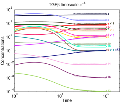
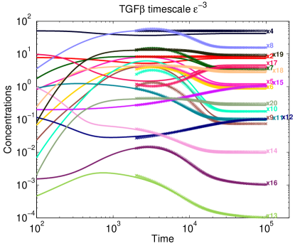
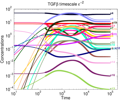
Figure 2: Comparison of numerical solutions obtained with the transformed TGF-$\beta$ model (continuous lines) and with slowest timescale reduced models (crosses). For each reduced model, a small number of variables (slow) follow ODEs. The initial values of these were chosen the same as the values computed with the full transformed model at a large enough time. The remaining fast variables were computed as functions of the slow variables. The large errors for a few species at times shorther than $10^{4}$ could be explained by lack of validity of the tropical equilibration used for the reduction at these shorter timescales, see also Figure 3.

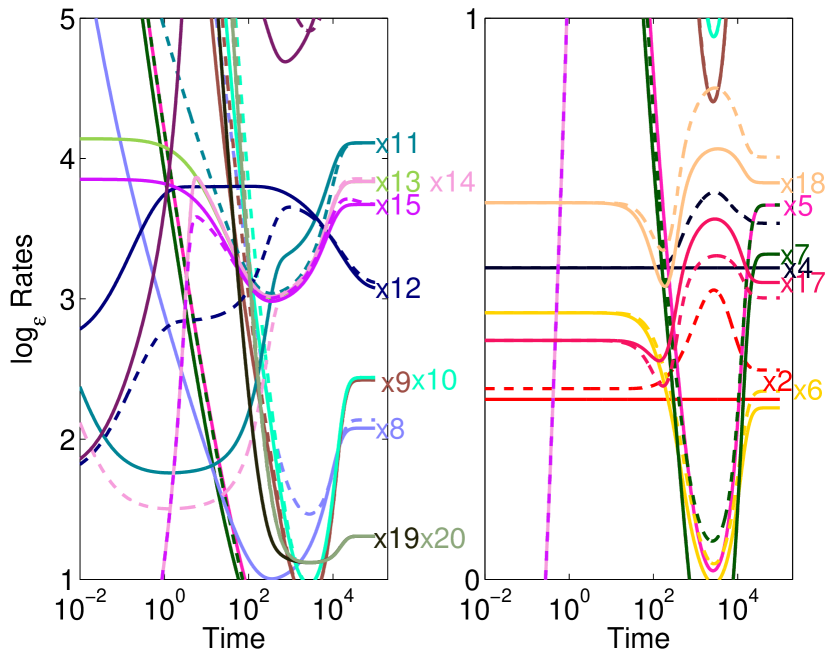
Figure 3: Testing tropical equilibration for various species of the transformed TGF-$\beta$ model. For each species we have plotted the $\log_{\epsilon}$ of positive (continuous line) and negative (dotted lines) rates producing and consuming these species, respectively. For tropically equilibrated species the two rates must have the same order (the $\log_{\epsilon}$ values should round up to the same integer for continuous and dotted curves of the same color). For times larger than $10^{4}$ this condition is valid for all species. For shorter times, a few species are not equilibrated. Furthermore, some rates change abruptly at these timescales, suggesting that different tropical equilibration solutions should be considered at shorter timescales.

References

- [1] Geoffroy Andrieux, Laurent Fattet, Michel Le Borgne, Ruth Rimokh, and Nathalie Théret. Dynamic regulation of Tgf- signaling by Tif1: a computational approach. PloS one, 7(3):e33761, 2012.
- [2] Rutherford Aris and RHS Mah. Independence of chemical reactions. Industrial & Engineering Chemistry Fundamentals, 2(2):90–94, 1963.
- [3] Pierre Auger, R Bravo de La Parra, Jean-Christophe Poggiale, E Sánchez, and L Sanz. Aggregation methods in dynamical systems and applications in population and community dynamics. Physics of Life Reviews, 5(2):79–105, 2008.
- [4] Vitalii Anvarovich Baikov, Rafail Kavyevich Gazizov, and Nail Hairullovich Ibragimov. Approximate symmetries. Matematicheskii Sbornik, 178(4):435–450, 1988.
- [5] Max Bodenstein. Eine theorie der photochemischen reaktionsgeschwindigkeiten. Zeitschrift für physikalische Chemie, 85(1):329–397, 1913.
- [6] Tristram Bogart, Anders Nedergaard Jensen, David Speyer, Bernd Sturmfels, and Rekha R. Thomas. Computing tropical varieties. J. Symb. Comput., 42(1–2):54–73, January–February 2007.
- [7] Ludwig Boltzmann. Lectures on gas theory. U. of California Press, Berkeley, CA, USA, 1964.
- [8] Pedro Toniol Cardin and Marco Antonio Teixeira. Fenichel theory for multiple time scale singular perturbation problems. SIAM Journal on Applied Dynamical Systems, 16(3):1425–1452, 2017.
- [9] Domitilla Del Vecchio, Alexander J Ninfa, and Eduardo D Sontag. Modular cell biology: retroactivity and insulation. Molecular systems biology, 4(1):161, 2008.
- [10] Aurélien Desoeuvres, Alexandru Iosif, Ovidiu Radulescu, Hamid Rahkooy, Matthias Seiß, and Thomas Sturm. A computational approach to complete exact and approximate conservation laws of chemical reaction networks. preprint, 2022.
- [11] Aurélien Desoeuvres, Peter Szmolyan, and Ovidiu Radulescu. Qualitative dynamics of chemical reaction networks: An investigation using partial tropical equilibrations. In Ion Petre and Andrei Păun, editors, Computational Methods in Systems Biology, pages 61–85, Cham, 2022. Springer International Publishing.
- [12] Justin Eilertsen and Santiago Schnell. The quasi-steady-state approximations revisited: Timescales, small parameters, singularities, and normal forms in enzyme kinetics. Mathematical biosciences, 325:108339, 2020.
- [13] Manfred Einsiedler, Mikhail Kapranov, and Douglas Lind. Non-archimedean amoebas and tropical varieties. 2006(601):139–157, 2006.
- [14] Martin Feinberg. Foundations of Chemical Reaction Network Theory, volume 202 of Applied Mathematical Sciences. Springer, 2019.
- [15] Martin Feinberg and Friedrich JM Horn. Dynamics of open chemical systems and the algebraic structure of the underlying reaction network. Chemical Engineering Science, 29(3):775–787, 1974.
- [16] Elisenda Feliu and Carsten Wiuf. Preclusion of switch behavior in networks with mass-action kinetics. Applied Mathematics and Computation, 219(4):1449–1467, 2012.
- [17] Elisenda Feliu and Carsten Wiuf. Simplifying biochemical models with intermediate species. Journal of the Royal Society Interface, 10(87):20130484, 2013.
- [18] Neil Fenichel. Geometric singular perturbation theory for ordinary differential equations. Journal of differential equations, 31(1):53–98, 1979.
- [19] Richard P Feynman, Robert B Leighton, and Matthew Sands. The Feynman lectures on physics, Vol. I: mainly mechanics, radiation, and heat, volume 1. Addison-Wesley, 1963.
- [20] Mark I Freidlin. Perturbation of systems with a first integral: Motion on the reeb graph. Journal of Statistical Physics, 189(3):36, 2022.
- [21] Ziomara P Gerdtzen, Prodromos Daoutidis, and Wei-Shou Hu. Non-linear reduction for kinetic models of metabolic reaction networks. Metabolic engineering, 6(2):140–154, 2004.
- [22] Alexander N Gorban, Iliya V Karlin, Patrick Ilg, and Hans Christian Öttinger. Corrections and enhancements of quasi-equilibrium states. Journal of non-newtonian fluid mechanics, 96(1-2):203–219, 2001.
- [23] Alexander N. Gorban and Ovidiu Radulescu. Dynamic and static limitation in multiscale reaction networks, revisited. In Advances in Chemical Engineering, volume 34 of Advances in Chemical Engineering, chapter 3, pages 103–173. Elsevier, 2008.
- [24] Alexander N Gorban, Ovidiu Radulescu, and Andrei Y Zinovyev. Asymptotology of chemical reaction networks. Chemical Engineering Science, 65(7):2310–2324, 2010.
- [25] Frank Hoppensteadt. On systems of ordinary differential equations with several parameters multiplying the derivatives. J. Differ. Equations, 5(1):106–116, January 1969.
- [26] AH Kara, FM Mahomed, and G Unal. Approximate symmetries and conservation laws with applications. International journal of theoretical physics, 38(9):2389–2399, 1999.
- [27] Niclas Kruff, Christoph Lüders, Ovidiu Radulescu, Thomas Sturm, and Sebastian Walcher. Algorithmic reduction of biological networks with multiple time scales. Mathematics in Computer Science, 15(3):499–534, 2021.
- [28] Martin Krupa and Peter Szmolyan. Extending geometric singular perturbation theory to nonhyperbolic points—fold and canard points in two dimensions. SIAM journal on mathematical analysis, 33(2):286–314, 2001.
- [29] François Lemaire and Alexandre Temperville. On defining and computing “good” conservation laws. In International Conference on Computational Methods in Systems Biology, pages 1–19. Springer, 2014.
- [30] Grigoriĭ L. Litvinov. Maslov dequantization, idempotent and tropical mathematics: A brief introduction. J. Math. Sci., 140(3):426–444, January 2007.
- [31] Diane Maclagan and Bernd Sturmfels. Introduction to tropical geometry. graduate studies in mathematics. 161, 2009.
- [32] Adam Mahdi, Antoni Ferragut, Claudia Valls, and Carsten Wiuf. Conservation laws in biochemical reaction networks. SIAM Journal on Applied Dynamical Systems, 16(4):2213–2232, 2017.
- [33] Vincent Noel, Dima Grigoriev, Sergei Vakulenko, and Ovidiu Radulescu. Tropical geometries and dynamics of biochemical networks application to hybrid cell cycle models. In J. Feret and A. Levchenko, editors, Proc. SASB 2011, volume 284 of ENTCS, pages 75–91. Elsevier, 2012.
- [34] Vincent Noel, Dima Grigoriev, Sergei Vakulenko, and Ovidiu Radulescu. Tropicalization and tropical equilibration of chemical reactions. In G. L. Litvinov and S. N. Sergeev, editors, Tropical and Idempotent Mathematics and Applications, volume 616 of Contemporary Mathematics, pages 261–277. AMS, 2014.
- [35] Vincent Noel, Dima Grigoriev, Sergei Vakulenko, and Ovidiu Radulescu. Tropicalization and tropical equilibration of chemical reactions. Tropical and Idempotent Mathematics and Applications, 616:261–277, 2014.
- [36] Emmy Noether. Invarianten beliebiger differentialausdrücke. Nachrichten von der Gesellschaft der Wissenschaften zu Göttingen, mathematisch-physikalische Klasse, 1918:37–44, 1918.
- [37] RE O’Malley. On initial value problems for nonlinear systems of differential equations with two small parameters. Archive for Rational Mechanics and Analysis, 40(3):209–222, 1971.
- [38] Mikhail I Rabinovich, Ramón Huerta, Pablo Varona, and Valentin S Afraimovich. Transient cognitive dynamics, metastability, and decision making. PLoS computational biology, 4(5):e1000072, 2008.
- [39] Ovidiu Radulescu. Tropical geometry of biological systems (invited talk). In Computer Algebra in Scientific Computing, LNCS 12291, pages 1–13. Springer, 2020.
- [40] Ovidiu Radulescu, Alexander N Gorban, Andrei Zinovyev, and Alain Lilienbaum. Robust simplifications of multiscale biochemical networks. BMC systems biology, 2(1):1–25, 2008.
- [41] Ovidiu Radulescu, Alexander N Gorban, Andrei Zinovyev, and Vincent Noel. Reduction of dynamical biochemical reactions networks in computational biology. Frontiers in genetics, 3:131, 2012.
- [42] Ovidiu Radulescu, Satya Swarup Samal, Aurélien Naldi, Dima Grigoriev, and Andreas Weber. Symbolic dynamics of biochemical pathways as finite states machines. In International Conference on Computational Methods in Systems Biology, pages 104–120. Springer, 2015.
- [43] Ovidiu Radulescu, Sergei Vakulenko, and Dima Grigoriev. Model reduction of biochemical reactions networks by tropical analysis methods. Math. Model. Nat. Pheno., 10(3):124–138, June 2015.
- [44] Shodhan Rao, Arjan van der Schaft, and Bayu Jayawardhana. A graph-theoretical approach for the analysis and model reduction of complex-balanced chemical reaction networks. Journal of Mathematical Chemistry, 51(9):2401–2422, 2013.
- [45] Satya S. Samal, Dima Grigoriev, Holger Fröhlich, and Ovidiu Radulescu. Analysis of reaction network systems using tropical geometry. In V. Gerdt, W. Koepf, W. Seiler, and E. Vorozhtsov, editors, Proc. CASC 2015, volume 9301 of LNCS, pages 424–439. Springer, 2015.
- [46] Satya Swarup Samal, Dima Grigoriev, Holger Fröhlich, Andreas Weber, and Ovidiu Radulescu. A geometric method for model reduction of biochemical networks with polynomial rate functions. Bulletin of Mathematical Biology, 77(12):2180–2211, 2015.
- [47] Satya Swarup Samal, Aurélien Naldi, Dima Grigoriev, Andreas Weber, Nathalie Théret, and Ovidiu Radulescu. Geometric analysis of pathways dynamics: Application to versatility of tgf- receptors. Biosystems, 149:3–14, 2016.
- [48] Friedrich Schlögl. Chemical reaction models for non-equilibrium phase transitions. Zeitschrift für physik, 253(2):147–161, 1972.
- [49] Klaus R Schneider and Thomas Wilhelm. Model reduction by extended quasi-steady-state approximation. Journal of mathematical biology, 40(5):443–450, 2000.
- [50] Klaus R. Schneider and Thomas Wilhelm. Model reduction by extended quasi-steady-state approximation. J. Math. Biol., 40(5):443–450, May 2000.
- [51] Stefan Schuster and Thomas Höfer. Determining all extreme semi-positive conservation relations in chemical reaction systems: a test criterion for conservativity. Journal of the Chemical Society, Faraday Transactions, 87(16):2561–2566, 1991.
- [52] Lee A. Segel and Marshall Slemrod. The quasi-steady-state assumption: A case study in perturbation. SIAM Rev., 31(3):446–477, September 1989.
- [53] Nikolai N Semenov. Some problems relating to chain reactions and to the theory of combustion. Nobel Lecture, pages 487–514, 1956.
- [54] Irina Surovtsova, Natalia Simus, Thomas Lorenz, Artjom König, Sven Sahle, and Ursula Kummer. Accessible methods for the dynamic time-scale decomposition of biochemical systems. Bioinformatics, 25(21):2816–2823, 2009.
- [55] Nathalie Theret, Jérôme Feret, Arran Hodgkinson, Pierre Boutillier, Pierre Vignet, and Ovidiu Radulescu. Integrative models for TGF- signaling and extracellular matrix. In Extracellular Matrix Omics, pages 209–225. Springer, 2020.
- [56] Andrei Nikolaevich Tikhonov. Systems of differential equations containing small parameters in the derivatives. Mat. Sb. (N. S.), 73(3):575–586, 1952.
- [57] Adelaida Borisovna Vasil’eva and Valentin Fedorovich Butuzov. Singularly perturbed equations in the critical case. Technical report, Wisconsin Univ-Madison Mathematics Research Center, 1980.
- [58] Oleg Viro. Dequantization of real algebraic geometry on logarithmic paper. In C. Casacuberta, R. M. Miró-Roig, J. Verdera, and S. Xambó-Descamps, editors, European Congress of Mathematics, volume 201 of Progress in Mathematics, pages 135–146. Springer, 2001.
- [59] James Wei and Charles D Prater. The structure and analysis of complex reaction systems. In Advances in Catalysis, volume 13, pages 203–392. Elsevier, 1962.
- [60] Stephen Wiggins. Normally hyperbolic invariant manifolds in dynamical systems, volume 105. Springer Science & Business Media, 1994.
- [61] GS v Yablonskii, VI Bykov, VI Elokhin, and AN Gorban. Kinetic models of catalytic reactions. Elsevier, 1991.
- [62] Fuzhen Zhang. The Schur complement and its applications, volume 4. Springer Science & Business Media, 2006.