Fibered $3$–manifolds and Veech groups

Abstract.

We study Veech groups associated to the pseudo-Anosov monodromies of fibers and foliations of a fixed hyperbolic 3-manifold. Assuming Lehmer’s Conjecture, we prove that the Veech groups associated to fibers generically contain no parabolic elements. For foliations, we prove that the Veech groups are always elementary.

1. Introduction

A pseudo-Anosov homeomorphism $f\colon S\to S$ on an orientable surface determines a complex structure and holomorphic quadratic differential, $(X,q)$, up to Teichmüller deformation, for which the vertical and horizontal foliations are the stable and unstable foliations of $f$. The pseudo-Anosov generates an infinite cyclic subgroup of the full group of orientation preserving affine homeomorphisms, ${\rm{Aff}}_{+}(X,q)$.

For a finite type surface $S$, we say that the pseudo-Anosov homeomorphism $f$ is lonely if $\langle f\rangle<{\rm{Aff}}_{+}(S,q)$ has finite index. The motivation for this paper is the following; see e.g. Hubert-Masur-Schmidt-Zorich [HMSZ06] and Lanneau [Lan17]

Conjecture 1.1 (Lonely p-As).

There exist lonely pseudo-Anosov homeomorphisms. In fact, lonely pseudo-Anosov homeomorphisms are generic.

There is not an agreed upon notion of “generic”, and some care must be taken: work of Calta [Cal04] and McMullen [McM03a, McM03b] shows that no pseudo-Anosov homeomorphism on a surface of genus $2$, with orientable stable/unstable foliation is lonely. In fact, in this case, not only are the pseudo-Anosov homeomorphisms not lonely, but their Veech groups always contain parabolic elements.

In this paper, we consider infinite families of pseudo-Anosov homeomorphism arising as follows; see §2.1. Suppose $f\colon S\to S$ is a pseudo-Anosov homeomorphism of a finite type surface $S$ and $M_{f}$ the mapping torus (which is hyperbolic by Thurston’s Hyperbolization Theorem [Ota98]). The connected cross sections of the suspension flow are organized by their cohomology classes (up to isotopy), which are primitive integral classes in the cone on the open fibered face $F\subset H^{1}(M,\mathbb{R})$ of the Thurston norm ball containing the Poincaré-Lefschetz dual of the fiber $S$. Given such an integral class $\alpha$, the first return map to the cross section $S_{\alpha}$ is a pseudo-Anosov homeomorphism $f_{\alpha}\colon S_{\alpha}\to S_{\alpha}$. When $b_{1}(M)>1$, there are infinitely many such pseudo-Anosov homeomorphisms; in fact, $|\chi(S_{\alpha})|$ is a linear function of $\alpha$, and hence tends to infinity with $\alpha$.

We let $\bar{\alpha}\in F$ denote the projection of the primitive integral class $\alpha$ in the cone over $F$, and let $F_{\mathbb{Q}}$ be the set of all such projections, which is precisely the (dense) set of rational points in $F$.

Question 1.2.

Given a fibered hyperbolic $3$–manifold and fibered face $F$, are the pseudo-Anosov homeomorphism $f_{\alpha}$ for $\bar{\alpha}\in F_{\mathbb{Q}}$ generically lonely?

We will provide two pieces of evidence that the answer to this question is ‘yes’. Write ${\rm{Aff}}_{+}(X_{\alpha},q_{\alpha})$ for the orientation preserving affine group containing $f_{\alpha}$; see §2.3 for more details.

Theorem 1.3.

Suppose $F$ is the fibered face of an orientable, fibered, hyperbolic $3$–manifold. Assuming Lehmer’s Conjecture, the set of $\bar{\alpha}\in F_{\mathbb{Q}}$ such that ${\rm{Aff}}_{+}(X_{\alpha},q_{\alpha})$ contains a parabolic element is discrete in $F$.

In certain examples, the set of classes whose associated Veech group contains parabolics is actually finite (again, assuming Lehmer’s conjecture); see Theorem 4.2. In §3 we describe some explicit computations that illustrate this finite set. If $M$ is the orientation cover of a non-orientable, fibered $3$–manifold, then the conclusion of Theorem 1.3 holds on the invariant cohomology of the covering involution without assuming the validity of Lehmer’s Conjecture; see Theorem 4.3.

Much of the defining structure survives for non-integral classes $\alpha\in F-F_{\mathbb{Q}}$; see §2.2 for details. Briefly, we first recall that every $\alpha\in F-F_{\mathbb{Q}}$ is represented by a closed $1$–form $\omega_{\alpha}$ which is positive on the vector field generating the suspension flow. The kernel of $\omega_{\alpha}$ is tangent to a foliation $\mathcal{F}_{\alpha}$, and the flow can be reparameterized to send leaves of $\mathcal{F}_{\alpha}$ to other leaves. There is no longer a first return time, but rather a higher rank abelian group of return times, $H_{\alpha}$, to any given leaf $S_{\alpha}$ of $\mathcal{F}_{\alpha}$. Work of McMullen [McM00] associates a leaf-wise complex structure and quadratic differential $(X_{\alpha},q_{\alpha})$ to each $\alpha\in F-F_{\mathbb{Q}}$ so that the leaf-to-leaf maps of the flow are all Teichmüller maps. For every leaf $S_{\alpha}$ of $\mathcal{F}_{\alpha}$, the return maps to $S_{\alpha}$ thus determine an isomorphism from $H_{\alpha}<\mathbb{R}$ to a subgroup we denote $H_{\alpha}^{{\rm{Aff}}}\!\!<{\rm{Aff}}_{+}(X_{\alpha},q_{\alpha})$, an abelian group of pseudo-Anosov elements. Our second piece of evidence for a positive answer to Question 1.2 is the following.

Theorem 1.4.

If $F$ is a fibered face of a closed, orientable, fibered, hyperbolic $3$–manifold, then for all $\alpha\in F-F_{\mathbb{Q}}$, and any leaf $S_{\alpha}$ of $\mathcal{F}_{\alpha}$, the abelian group $H_{\alpha}^{{\rm{Aff}}}\!\!<{\rm{Aff}}_{+}(X_{\alpha},q_{\alpha})$ has finite index.

For $\alpha\in F-F_{\mathbb{Q}}$, the leaves $S_{\alpha}$ are infinite type surfaces. In general, there is much more flexibility in constructing affine groups for infinite type surfaces, and exotic groups abound. Indeed, work of Przyticki-Schmithusen-Valdez [PSV11] and Ramírez-Valdez [RMV17] proves that any countable subgroup of ${\rm{GL}}_{2}(\mathbb{R})$ without contractions is the derivative-image of some affine group. (See also Bowman [Bow13] for a “naturally occurring” lonely pseudo-Anosov homeomorphism on an infinite type surface of finite area.) Theorem 1.4 says that for the leaves $S_{\alpha}$ of the foliations and their associated quadratic differentials, the situation is much more rigid.

Acknowledgements

The authors would like to thank Erwan Lanneau, Livio Liechti, Alan Reid, and Ferrán Valdez for helpful conversations, and to the anonymous referee for suggestions that improved the readability. We are particularly grateful to Liechti for suggesting Theorem 4.3. The first author was partially supported by NSF grant DMS-2106419. The second author was partially supported by NSERC Discovery grant, RGPIN 06486. The fifth author was partially supported by an NSERC-PDF Fellowship.

2. Definitions and background

2.1. Fibered $3$–manifolds

Here we explain the set up and background for our work in more detail. For a pseudo-Anosov homeomorphism $f\colon S\to S$ of an orientable, finite type surface $S$, let $\lambda(f)$ denote its stretch factor (also called its dilatation); see [FLP79]. We write

$$M=M_{f}=S\times[0,1]/(x,1)\sim(f(x),0)$$

to denote the mapping torus of the pseudo-Anosov homeomorphism $f$. The suspension flow $\psi_{s}$ of $f$ is generated by the vector field $\xi=\frac{\partial}{\partial t}$, where $t$ is the coordinate on the $[0,1]$ factor. Alternatively, we have the local flow of the same name $\psi_{s}(x,t)=(x,t+s)$ on $S\times[0,1]$, defined for $t,s+t\in[0,1]$, which descends to the suspension flow.

A cross section (or just section) of the flow is a surface $S_{\alpha}\subset M$ transverse to $\xi$, such that for all $x\in S_{\alpha}$, $\psi_{s}(x)\in S_{\alpha}$ for some $s>0$. If $s(x)>0$ is the smallest such number, then the first return map of $\psi_{s}$ is the map $f_{\alpha}\colon S_{\alpha}\to S_{\alpha}$ defined by $f_{\alpha}(x)=\psi_{s(x)}(x)$ for $x\in S_{\alpha}$. Note that $S(=S\times\{0\})\subset M$ is a section, and the first return map to $S$ is precisely the map $f=\psi_{1}|_{S}$.

Cutting open along an arbitrary section $S_{\alpha}$ we get a product $S_{\alpha}\times[0,1]$ where the slices $\{x\}\times[0,1]$ are arcs of flow lines. Thus, $M$ can also be expressed as the mapping torus of $f_{\alpha}$, or alternatively, $M$ fibers over the circle with monodromy $f_{\alpha}$. Up to isotopy, the fiber $S_{\alpha}$ is determined by its Poincaré-Lefschetz dual cohomology class $\alpha=[S_{\alpha}]\in H^{1}(M;\mathbb{Z})\subset H^{1}(M;\mathbb{R})=H^{1}(M)$. To see how these are organized, we first recall the following theorem of Thurston [Thu86]

Theorem 2.1.

For $M=M_{f}$ as above, there is a finite union of open, convex, polyhedral cones $\mathcal{C}_{1},\ldots,\mathcal{C}_{k}\subset H^{1}(M)$ such that $\alpha\in H^{1}(M;\mathbb{Z})$ is dual to a fiber in a fibration over $S^{1}$ if and only if $\alpha\in\mathcal{C}_{j}$ for some $j$. Moreover, there is a norm $\|\cdot\|_{T}$ on $H^{1}(M)$ so that for each $\mathcal{C}_{j}$, $\|\cdot\|_{T}$ restricted to $\mathcal{C}_{j}$ is linear, and if $\alpha\in\mathcal{C}_{j}\cap H^{1}(M;\mathbb{Z})$ then $\|\alpha\|_{T}$ is the negative of the Euler characteristic of the fiber dual to $\alpha$.

The unit ball $\mathfrak{B}$ of $\|\cdot\|_{T}$ is a polyhedron, and each $\mathcal{C}_{j}$ is the cone over the interior of a top dimensional face $F_{j}$ of $\mathfrak{B}$.

The cones in the theorem are called the fibered cones of $M$ and the $F_{j}$ the fibered faces of $\mathfrak{B}$. It follows from Thurston’s proof of Theorem 2.1 that each of the sections $S_{\alpha}$ of $(\psi_{s})$ described above must lie in a single one of the fibered cones $\mathcal{C}$ over a fibered face $F$. The following theorem elaborates on this, combining results of Fried from [Fri83, Fri82].

Theorem 2.2.

For $M=M_{f}$ as above, there is a fibered cone $\mathcal{C}\subset H^{1}(M)$ such that $\alpha\in H^{1}(M;\mathbb{Z})$ is dual to a section of $(\psi_{s})$ if and only if $\alpha\in\mathcal{C}$. Moreover, there is a function $\mathfrak{h}\colon\mathcal{C}\to\mathbb{R}_{+}$ which is continuous, convex, and homogenous of degree $-1$, with the following properties.

• For any $\alpha\in\mathcal{C}\cap H^{1}(M;\mathbb{Z})$, $f_{\alpha}$ is pseudo-Anosov and $\mathfrak{h}(\alpha)=\log(\lambda(f_{\alpha}))$.

• For any $\{\alpha_{n}\}\subset\mathcal{C}$ with $\alpha_{n}\to\partial\mathcal{C}$, we have $\mathfrak{h}(\alpha_{n})\to\infty$;

We let $\mathcal{C}_{\mathbb{Z}}\subset\mathcal{C}$ denote the primitive integral classes in the fibered cone $\mathcal{C}$; that is, the integral points which are not nontrivial multiples of another element of $H^{1}(M;\mathbb{Z})$. These correspond precisely to the connected sections of $(\psi_{s})$.

McMullen [McM00] refined the analysis of $\mathfrak{h}$, proving for example that it is actually real-analytic. For this, he computed the stretch factors using his Teichmüller polynomial $\Theta_{\mathcal{C}}$. This polynomial

$$\Theta_{\mathcal{C}}=\sum_{g\in G}a_{g}g$$

is an element of the group ring $\mathbb{Z}[G]$ where $G=H_{1}(M;\mathbb{Z})/\text{torsion}$. For $\alpha\in\mathcal{C}_{\mathbb{Z}}$, the specialization of the Teichmüller polynomial is

$$\Theta_{\mathcal{C}}^{\alpha}(t)=\sum_{g\in G}a_{g}t^{\alpha(g)}\in\mathbb{Z}[t^{\pm 1}]$$

where we view $\alpha\in H^{1}(M;\mathbb{Z})\cong\rm{Hom}(G;\mathbb{Z})$. Further, $G\cong H\oplus\mathbb{Z}$ where $H=\text{Hom}(H^{1}(S,\mathbb{Z})^{f},\mathbb{Z})\cong\mathbb{Z}^{m}$ and $H^{1}(S,\mathbb{Z})^{f}$ are the $f$–invariant cohomology classes. So we can regard $\Theta_{\mathcal{C}}$ as a Laurent polynomial on the generators $x_{1},x_{2},\ldots,x_{m}$ of $H$ and the generator $u$ of $\mathbb{Z}$. Then specialization to the dual of an element $(a_{1},a_{2},\ldots,a_{m},b)\in\mathcal{C}\cap H^{1}(M;\mathbb{Z})$ amounts to setting $x_{i}=t^{a_{i}}$ for $1\leq i\leq m$ and $u=t^{b}$. McMullen proves that the specializations and the pseudo-Anosov first return maps are related by the following.

Theorem 2.3.

For any $\alpha\in\mathcal{C}_{\mathbb{Z}}$, the stretch factor $\lambda(f_{\alpha})$ is a root of $\Theta_{\mathcal{C}}^{\alpha}$ with the largest modulus.

Combining the linearity of $\|\cdot\|_{T}$ on $\mathcal{C}$ together with the homogeneity of $\mathfrak{h}$, we have the following observation of McMullen; see [McM00].

Corollary 2.4.

The function $\alpha\mapsto\|\alpha\|_{T}\mathfrak{h}(\alpha)$ is continuous and constant on rays from $0$. In particular, if $K\subset\mathcal{C}$ is any compact subset, then $\|\cdot\|_{T}\mathfrak{h}(\cdot)$ is bounded on $\mathbb{R}_{+}K$.

The key corollary for us is the following, also observed by McMullen from the same paper.

Corollary 2.5.

If $\{\alpha_{n}\}_{n}\subset\mathcal{C}_{\mathbb{Z}}$ is any infinite sequence of distinct elements, then $|\chi(S_{\alpha_{n}})|\to\infty$ and if the rays $\mathbb{R}_{+}\alpha_{n}$ do not accumulate on $\partial\mathcal{C}$, then

$$\log(\lambda(f_{\alpha_{n}}))\asymp\frac{1}{|\chi(S_{\alpha_{n}})|}.$$

In particular, $\lambda(f_{\alpha_{n}})\to 1$.

Remark 2.6.

One can sometimes promote the final conclusion to any infinite sequence of distinct elements, without the assumption about non-accumulation to $\partial\mathcal{C}$; see the examples in §3. This is not always the case, and the accumulation set of stretch factors can be fairly complicated, as described by work of Landry-Minsky-Taylor [LMT21].

2.2. Foliations in the fibered cone

Fried’s work described above [Fri83, Fri82] implies that any $\alpha\in\mathcal{C}$ may be represented by a closed $1$–form $\omega_{\alpha}$ for which $\omega_{\alpha}(\xi)>0$ at every point of $M$. For integral classes, $\omega_{\alpha}$ is the pull-back of the volume form from the fibration over the circle $\mathbb{R}/\mathbb{Z}$, and in general, $\omega_{\alpha}$ is a convex combination of such $1$–forms. The kernel of $\omega_{\alpha}$ defines a foliation $\mathcal{F}_{\alpha}$ transverse to $\xi$ whose leaves are injectively immersed surfaces $S_{\alpha}\subset M$. We consider the reparameterized flow $\{\psi_{s}^{\alpha}\}$ defined by scaling the generating vector field $\xi$ by $\xi/\omega_{\alpha}(\xi)$. Then for every leaf $S_{\alpha}\subset M$ of $\mathcal{F}_{\alpha}$ and for every $s\in\mathbb{R}$, the image by the flow $\psi_{s}^{\alpha}(S_{\alpha})$ is another leaf of $\mathcal{F}_{\alpha}$. The subgroup $H_{\alpha}<\mathbb{R}$ mentioned in the introduction is precisely the set of return times of $\psi_{s}^{\alpha}$ to $S_{\alpha}$. As such, $H_{\alpha}$ acts on $S_{\alpha}$ so that $s\in H_{\alpha}$ acts by $s\cdot x=\psi_{s}^{\alpha}(x)$, for all $x\in S_{\alpha}$.

The group $H_{\alpha}\cong\mathbb{Z}^{n}$ for some $n=n_{\alpha}\leq b_{1}(M)$, and can alternatively be defined as the set of periods of $\alpha$ (i.e. the $\alpha$–homomorphic image of $H_{1}(M;\mathbb{Z})$). A leaf $S_{\alpha}$ is a closed surface, and in fact a fiber as above if and only if $n_{\alpha}=1$ in which case $H_{\alpha}$ is a discrete subgroup of $\mathbb{R}$ and $\bar{\alpha}\in F_{\mathbb{Q}}$. On the other hand, $n_{\alpha}\geq 2$ if and only if the group of return times $H_{\alpha}$ is indiscrete, and so $S_{\alpha}$ is dense in $M$.

2.3. Teichmüller flows and Veech groups

In [McM00], McMullen defines a conformal structure and quadratic differential, $(X_{\alpha},q_{\alpha})$, on the leaves $S_{\alpha}$ of the foliation $\mathcal{F}_{\alpha}$, for all $\alpha\in\mathcal{C}$, with the following properties. For each $s\in\mathbb{R}$ and leaf $S_{\alpha}$, the leaf-to-leaf map $\psi_{s}^{\alpha}\colon S_{\alpha}\to\psi_{s}^{\alpha}(S_{\alpha})$ is a Teichmüller map with initial/terminal quadratic differentials given by $q_{\alpha}$ on the respective leaves. In fact, there exists some $K_{\alpha}>1$ so that $\psi_{s}^{\alpha}$ is a $K_{\alpha}^{|s|}$–Teichmüller map, and hence $K_{\alpha}^{2|s|}$–quasi-conformal.

Remark 2.7.

The notation $(X_{\alpha},q_{\alpha})$ is somewhat ambiguous: this really denotes a family of structures, one on every leaf, though we abuse notation and also use this same notation to denote the restriction to any given leaf.

The vertical and horizontal foliations of $q_{\alpha}$ on the leaves $S_{\alpha}$ of $\mathcal{F}_{\alpha}$ are obtained by intersecting with a fixed singular foliation on the $3$–manifold; namely, the suspension of the unstable/stable foliations for the original pseudo-Anosov homeomorphism $f$. In particular, the cone points (i.e. zeros) of $q_{\alpha}$ are precisely the intersections of $S_{\alpha}$ with the $\psi_{s}$–flowlines through the cone points on the original surface $S$. Consequently, the cone points are isolated, and the cone angles are bounded by those of the original surface, and are hence bounded independent of $\alpha$.

For $s\in H_{\alpha}$, $\psi_{s}^{\alpha}\colon S_{\alpha}\to S_{\alpha}$ is (a remarking) of the Teichmüller map, and thus an affine pseudo-Anosov homeomorphism with respect to $q_{\alpha}$. In this way, we obtain an isomorphism from $H_{\alpha}$ to a subgroup $H_{\alpha}^{{\rm{Aff}}}<{\rm{Aff}}_{+}(X_{\alpha},q_{\alpha})$, the group of orientation preserving affine homeomorphisms of the leaf $S_{\alpha}$ with respect to $(X_{\alpha},q_{\alpha})$. The derivative with respect to the preferred coordinates defines a map

$$D_{\alpha}\colon{\rm{Aff}}_{+}(X_{\alpha},q_{\alpha})\to{\rm{GL}}_{2}^{+}(\mathbb{R})/\pm I,$$

which is called the Veech group of $(X_{\alpha},q_{\alpha})$. A parabolic element of ${\rm{Aff}}_{+}(X_{\alpha},q_{\alpha})$ is one whose image by $D_{\alpha}$ is parabolic.

Remark 2.8.

The preferred coordinates for a quadratic differential are only defined up to translation and rotation through angle $\pi$, so the derivative is only defined up to sign. If all affine homeomorphisms are area preserving (e.g. if the surface has finite area) then the derivative maps to ${\rm{PSL}}_{2}(\mathbb{R})=\rm SL_{2}(\mathbb{R})/\pm I$.

Since the vertical/horizontal foliations are the stable/unstable foliations, the image of $H_{\alpha}^{\rm{Aff}}$, which we denote $H_{\alpha}^{D}=D_{\alpha}(H_{\alpha}^{\rm{Aff}})$ is contained in the diagonal subgroup of ${\rm{PSL}}_{2}(\mathbb{R})$:

$$H_{\alpha}^{D}<\Delta=\left\{\left.\left(\begin{array}[]{cc}a&0\\ 0&\frac{1}{a}\end{array}\right)\in\rm SL_{2}(\mathbb{R})\,\,\right|\,\,a>0\,\,\right\}/\pm I.$$

Define ${\rm SAff}(X_{\alpha},q_{\alpha})<{\rm{Aff}}_{+}(X_{\alpha},q_{\alpha})$ to be the area preserving subgroup of orientation preserving affine homeomorphisms; this is the preimage of ${\rm{PSL}}_{2}(\mathbb{R})$ under $D_{\alpha}$. In particular, $H_{\alpha}^{\rm{Aff}}<{\rm SAff}(X_{\alpha},q_{\alpha})$.

2.4. Trace fields

A number field is totally real if the image of every embedding into $\mathbb{C}$ lies in $\mathbb{R}$. Hubert-Lanneau [HL06] proved the following.

Theorem 2.9.

If a nonelementary Veech group contains a parabolic element, then the trace field is totally real.

A pseudo-Anosov $f$ being lonely implies that there are no parabolic elements in the Veech group, but not conversely; see [HLM09].

McMullen [McM03b, Corollary 9.6] proved the following fact about the trace field of a Veech group; see also Kenyon-Smillie [KS00].

Theorem 2.10.

The trace field of a Veech group containing a pseudo-Anosov is generated by the trace of that pseudo-Anosov. That is, the trace field is given by $\mathbb{Q}(\lambda(f)+\lambda(f)^{-1})$.

Thus, this trace field is totally real precisely when the trace of the pseudo-Anosov has only real Galois conjugates.

Remark 2.11.

Theorems 2.9 and 2.10 are proved for complex structures with an abelian differential, rather than a quadratic differential. The proof of Theorem 2.9 for the more general case of quadratic differentials follows verbatim since the key ingredient is the so-called Thurston-Veech construction, which works for both quadratic differentials and abelian differentials (see [Thu88, §6]). Theorem 2.10 for quadratic differentials follows from the case of abelian differentials since every affine homeomorphism lifts to the canonical $2$–fold cover where a quadratic differential pulls back to a square of an abelian differential, and thus the preimage of the Veech group of the original surface in $\rm SL_{2}(\mathbb{R})$ is contained in the Veech group for the abelian differential.

2.5. Lehmer’s Conjecture

Theorem 1.3 is dependent on the validity of what is known as Lehmer’s conjecture [Leh33] though Lehmer did not actually conjecture the statement we will use. See [Smy08]. To state this conjecture, we need the following.

Definition 2.12.

Let $p(x)\in\mathbb{C}[x]$ with factorization over $\mathbb{C}$

$$p(x)=a_{0}\prod_{i=1}^{m}(x-\gamma_{i}).$$

The Mahler measure of $p$ is

$$\mathcal{M}(p)=\left|a_{0}\right|\prod_{i=1}^{m}(\max{1,|\gamma_{i}|}).$$

With this definition, we state the conjecture we assume.

Conjecture 2.13 (Lehmer).

There is a constant $\mu>1$ such that for every $p(x)\in\mathbb{Z}[x]$ with a root not equal to a root of unity $\mathcal{M}(p)\geq\mu$.

Lehmer’s Conjecture is known in some special cases, including the following result of Schinzel [Sch75] which will be important in the proof of Theorem 4.3.

Theorem 2.14.

If $p(t)$ is the minimal polynomial for an algebraic integer not equal to $0$ or $\pm 1$, all of whose roots are real, then

$$\mathcal{M}(p)\geq\left(\tfrac{1+\sqrt{5}}{2}\right)^{\deg(p)/2}.$$

3. Examples

Here we provide examples of fibered faces of fibered 3-manifolds and examine arithmetic features of the Veech groups of the corresponding pseudo-Anosov homeomorphisms.

3.1. Example 1

Let $\beta=\sigma_{1}\sigma_{2}^{-1}$ be an element of the braid group $B_{3}$ on three strands (viewed as the mapping class group of a four-punctured sphere, $S$), where $\sigma_{1}$ and $\sigma_{2}$ denote the standard generators. Let $M$ denote the mapping torus of $\beta$. McMullen computes the Teichmüller polynomial for this manifold in detail in [McM00]. See also Hironaka [Hir10].

Since $\beta$ permutes the strands of the braid cyclically, $b_{1}(M)=2$. Choosing appropriate bases, we obtain an isomorphism $H^{1}(M;\mathbb{Z})\cong\mathbb{Z}^{2}$ so that the starting fiber surface $S$ is dual to $(0,1)$, the fibered cone is

$$\mathcal{C}=\{(a,b)\in\mathbb{R}^{2}:b>0,-b<a<b\}$$

and the Teichmüller polynomial for this cone is

$$\Theta_{\mathcal{C}}(x,u)=u^{2}-u(x+1+x^{-1})-1.$$

Specialization to an integral class $(a,b)\in\mathcal{C}_{\mathbb{Z}}$ equates to setting $x=t^{a}$ and $u=t^{b}$ and yields

$$\Theta_{\mathcal{C}}^{(a,b)}(t)=\Theta_{\mathcal{C}}(t^{a},t^{b})=t^{2b}-t^{b+a}-t^{b}-t^{b-a}+1.$$

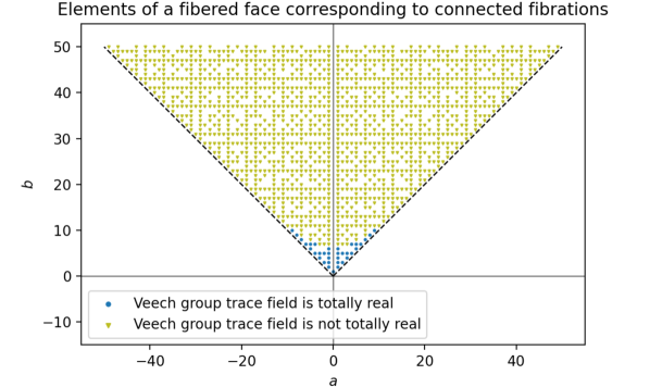
We used the mathematics software system SageMath [S⁺21] to factor $\Theta_{\mathcal{C}}^{(a,b)}(t)$ for all primitive integral pairs $(a,b)\in\mathcal{C}$ with $b<50$, to determine the stretch factors $\lambda_{(a,b)}$ of the corresponding monodromies and their minimal polynomials. We then computed the conjugates of the corresponding traces, $\lambda_{(a,b)}+1/\lambda_{(a,b)}$, to determine whether the trace field of each associated Veech group is totally real. The results are shown in Figure 1. Recall that by Theorem 2.9, when this trace field is not totally real, the Veech group has no parabolic elements.

These computations suggest that there are only finitely many pairs $(a,b)$ where the trace field is not totally real. This is not a coincidence as we will see below. For this, we record the following improvement on Corollary 2.5 for the cone $\mathcal{C}$ for this example.

Lemma 3.1.

For any sequence $\alpha_{n}=(a_{n},b_{n})\in{\mathcal{C}}_{\mathbb{Z}}$ of distinct elements, we have $\lambda(f_{\alpha_{n}})\to 1$.

Proof.

Since $\mathfrak{h}$ is convex, the maximum value of $\mathfrak{h}(a,b)=\log(\lambda(f_{(a,b)}))$, for points $(a,b)\in\mathcal{C}_{\mathbb{Z}}$ and a fixed $b$, occurs at either $(b-1,b)$ or $(1-b,b)$.

First we consider the points of the form $(b-1,b)$. The specialization of $\Theta_{\mathcal{C}}$ in this case takes the form

$$\Theta_{\mathcal{C}}^{(b-1,b)}(t)=t^{2b}-t^{2b-1}-t^{b}-t+1.$$

Recall that $\lambda_{b}=\lambda(f_{(b-1,b)})>1$. As $b\to\infty$, we claim that $\lambda_{b}\to 1$. Suppose instead that the sequence is bounded below by $1+\epsilon$, for $\epsilon>0$ on some subsequence. Then in this subsequence we have

$$\Theta_{\mathcal{C}}^{(b-1,b)}(\lambda_{b}) =\lambda_{b}^{2b}(1-\lambda_{b}^{-1}-\lambda_{b}^{-b}-\lambda_{b}^{1-2b})+1$$

$$\geq(1+\epsilon)^{2b}\left(1-(1+\epsilon)^{-1}-(1+\epsilon)^{-b}-(1+\epsilon)^{1-2b}\right)$$

The first factor on the right hand side tends to infinity when $b$ does, while the second factor tends toward $1-(1+\epsilon)^{-1}=\epsilon/(1+\epsilon)>0$. This implies that $\Theta_{\mathcal{C}}^{(b-1,b)}(\lambda_{b})$ approaches infinity, whereas instead it is identically equal to 0. This contradiction proves the claim.

For points of the form $(1-b,b)$, the specialization takes the form

$$\Theta_{\mathcal{C}}^{(1-b,b)}(t)=t^{2b}-t-t^{b}-t^{2b-1}+1=\Theta_{\mathcal{C}}^{(b-1,b)}(t).$$

Therefore, $\lambda(f_{(1-b,b)})=\lambda(f_{(b-1,b)})=\lambda_{b}$ and as $b\to\infty$, these both tend to $1$. ∎

Figure 1. Primitive integral elements in a fibered cone for the mapping torus of the three-strand braid $\sigma_{1}\sigma_{2}^{-1}$. Elements marked with green triangles have corresponding Veech group with trace field that is not totally real.

One of the difficulties in the proof of Theorem 1.3 is understanding the degrees of the trace field. This is complicated by the fact that the Teichmüller polynomial need not be irreducible in general. For example, when specialized to $(a,b)=(9,14)$, the Teichmüller polynomial in this example splits into the cyclotomic polynomials $t^{2}-t+1$ and $t^{4}-t^{2}+1$, plus the minimal polynomial of the corresponding stretch factor. However, in other cases, such as the specialization to $(a,b)=(5,14)$, the Teichmüller polynomial remains irreducible. We refer the reader to [FG22] for more on the factorizations of the specialized polynomials in the example above. As we will see in the example below, the Teichmüller polynomial also sometimes admits additional non-cyclotomic factors aside from the minimal polynomial of the corresponding stretch factor.

3.2. Example 2

Let $\beta^{\prime}=\beta^{2}$, for $\beta$ from the preceding example. Let $M^{\prime}$ denote the mapping torus on $\beta^{\prime}$ and ${\theta^{\prime}}_{\mathcal{C}^{\prime}}$ the Teichmüller polynomial of the fibered cone $\mathcal{C}^{\prime}$ containing the dual of $\beta^{\prime}$. Here we will observe three different splitting behaviors of specializations of the Teichmüller polynomial. In particular, we see that certain specializations of ${\theta^{\prime}}_{\mathcal{C}^{\prime}}$ split into multiple non-cyclotomic factors, limiting what information can be derived about conjugates of the corresponding stretch factors and their traces by looking at the collection of all roots of ${\theta^{\prime}}_{\mathcal{C}^{\prime}}$.

The Teichmüller polynomial here is

$${\theta^{\prime}}_{\mathcal{C}^{\prime}}(x,u)=u^{2}-u(x^{2}+2x+1+2x^{-1}+x^{-2})+1$$

over the cone

$$\mathcal{C}=\{(a,b)\in\mathbb{R}^{2}:b>0,-b/2<a<b/2\}.$$

The specialization to $(a,b)=(6,17)$ is irreducible over $\mathbb{Z}$:

$$t^{34}-t^{29}-2t^{23}-t^{17}-2t^{11}-t^{5}+1,$$

while the specialization to $(a,b)=(7,17)$ splits as a cyclotomic and non-cyclotomic factor:

$$(t^{4}+t^{3}+t^{2}+t+1)(t^{30}-t^{29}-t^{27}+t^{26}+t^{25}-t^{24}-t^{22}+t^{21}-t^{20}+t^{19}-t^{17}+t^{16}\\ -t^{15}+t^{14}-t^{13}+t^{11}-t^{10}+t^{9}-t^{8}-t^{6}+t^{5}+t^{4}-t^{3}-t+1),$$

and the specialization to $(a,b)=(7,18)$ has multiple non-cyclotomic factors:

$$(t^{2}-t+1)(t^{4}+t^{3}+t^{2}+t+1)(t^{12}-t^{9}-t^{8}+t^{7}+t^{6}+t^{5}-t^{4}-t^{3}+1)(t^{18}-t^{16}-t^{9}-t^{2}+1).$$

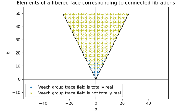
Figure 2 shows whether the Veech groups corresponding to elements of $\mathcal{C}^{\prime}$ have totally real trace field. For all three specializations described in this example, the corresponding Veech group trace field is not totally real.

The analog to Lemma 3.1 holds in this example as well. $M^{\prime}$ is a 2-fold cover of $M$ so the stretch factors in $\mathcal{C}_{\mathbb{Z}}^{\prime}$ are at most squares of the stretch factors in $\mathcal{C}_{\mathbb{Z}}$.

Figure 2. Primitive integral elements in a fibered cone for the mapping torus of the three-strand braid $(\sigma_{1}\sigma_{2}^{-1})^{2}$. Elements marked with green triangles have a not totally real corresponding Veech group.

4. Most Veech groups have no parabolics

We are now ready for the proof of the first theorem from the introduction.

Theorem 1.3. Suppose $F$ is the fibered face of an orientable, fibered, hyperbolic $3$–manifold. Assuming Lehmer’s Conjecture, the set of $\bar{\alpha}\in F_{\mathbb{Q}}$ such that ${\rm{Aff}}_{+}(X_{\alpha},q_{\alpha})$ contains a parabolic element is discrete in $F$.

Proof.

Consider any sequence of distinct elements $\alpha_{n}$ in $\mathcal{C}_{\mathbb{Z}}$ such that $\bar{\alpha}_{n}$ does not accumulate on $\partial F$. We need to show that ${\rm{Aff}}(X_{\alpha},q_{\alpha_{n}})$ contains a parabolic for at most finitely many $n$. According to Theorem 2.9, it suffices to prove that the trace field is totally real for at most finitely many $n$. Setting $\lambda_{n}=\lambda(f_{\alpha_{n}})$, Theorem 2.10 implies that the trace field of ${\rm{Aff}}(X_{\alpha_{n}},q_{\alpha_{n}})$ is $\mathbb{Q}(\lambda_{n}+\lambda_{n}^{-1})$.

Next, let $N$ be the number of terms of the Teichmüller polynomial, $\Theta_{\mathcal{C}}$ for $\mathcal{C}$. The stretch factor $\lambda_{n}$ is the largest modulus root of the specialization $\Theta_{\mathcal{C}}^{\alpha_{n}}(t)$ by Theorem 2.3. We observe that this polynomial has no more nonzero terms than $\Theta_{\mathcal{C}}$, and thus has at most $N$ terms. Descartes’s rule of signs implies that the number of real roots of $\Theta_{\mathcal{C}}^{\alpha_{n}}$ is at most $2N-2$.

Suppose that $p_{n}(t)$ is the minimal polynomial of $\lambda_{n}$, which is thus a factor of $\Theta_{\mathcal{C}}^{\alpha_{n}}(t)$ (up to powers of $t$, which we will ignore). In particular, note that $\lambda_{n}$ bounds the modulus of all other roots of $p_{n}(t)$. The stretch factors are always algebraic integers, and hence $p_{n}(t)$ is monic. The Mahler measure is therefore the product of the moduli of the roots outside the unit circle. There are at most $2N-2$ real roots of $\Theta_{\mathcal{C}}^{\alpha_{n}}(t)$, and hence the same is true of $p_{n}(t)$. Write

$$\mathcal{M}(p_{n})=A_{n}B_{n}$$

where $A_{n}$ is the product of the moduli of the real roots and $B_{n}$ is the product of the moduli of the non-real roots outside the unit circle (and $1$ if there are none). Thus, we have

(1) $$A_{n}\leq\lambda_{n}^{2N-2}.$$

Now, as $n\to\infty$, we have $|\chi(S_{\alpha_{n}})|=\|\alpha_{n}\|_{T}\to\infty$ as $n\to\infty$. Since $\bar{\alpha}_{n}$ does not accumulate on $\partial F$, Corollary 2.5 implies $\lambda_{n}=\lambda(f_{\alpha_{n}})\to 1$. By (1), it follows that $A_{n}\to 1$ as $n\to\infty$. Since we are assuming Lehmer’s Conjecture, it follows that $B_{n}>1$ for all but finitely many $n$. That is, there is at least one non-real root $\zeta_{n}$ of $p_{n}(t)$ outside the unit circle. (In fact, the number of such roots tends to infinity linearly with $|\chi(S_{\alpha_{n}})|$ since $\lambda_{n}$ has the maximum modulus of any root of $p_{n}(t)$).

Therefore, for all but finitely many $n$, the embedding of $\mathbb{Q}(\lambda_{n}+\lambda_{n}^{-1})$ to $\mathbb{C}$ sending $\lambda_{n}+\lambda_{n}^{-1}$ to $\zeta_{n}+\zeta_{n}^{-1}$ has non-real image, since $\zeta_{n}$ is non-real and lies off the unit circle. Therefore, $\mathbb{Q}(\lambda_{n}+\lambda_{n}^{-1})$ is totally real for at most finitely many $n$, as required. ∎

Remark 4.1.

The proof of Theorem 1.3 follows a strategy of Craig Hodgson, [Hod], for understanding trace fields under hyperbolic Dehn filling.

The key ingredient is that for sequences $\{\alpha_{n}\}$ in $\mathcal{C}_{\mathbb{Z}}$, we have $\lambda(f_{\alpha_{n}})\to 1$. Sometimes this happens for any sequence of distinct elements in the cone, and then one obtains the following stronger result.

Theorem 4.2.

Suppose $F$ is the fibered face of an orientable, fibered, hyperbolic $3$–manifold and that $1$ is the only accumulation point of the set

$$\{\lambda(f_{\alpha})\mid\bar{\alpha}\in F_{\mathbb{Q}}\}.$$

Assuming Lehmer’s Conjecture, the set of $\bar{\alpha}\in F_{\mathbb{Q}}$ such ${\rm{Aff}}_{+}(X_{\alpha},q_{\alpha})$ contains a parabolic element is finite.

Proof.

This is exactly the same as the proof of Theorem 1.3, except that the assumption that $1$ is the only accumulation point of $\{\lambda(f_{\alpha})\mid\bar{\alpha}\in F_{\mathbb{Q}}\}$ replaces the references to Corollary 2.5, and does away with the requirement that $\bar{\alpha}_{n}$ does not accumulate on $\partial F$. ∎

Returning to the examples from Section 3, Lemmas 3.1 and the discussion in both implies that the hypotheses of Theorem 4.2 are satisfied. Thus only finitely many elements $\alpha\in\mathcal{C}_{\mathbb{Z}}$ are such that ${\rm{Aff}}_{+}(X_{\alpha},q_{\alpha})$ can contain parabolics. We refer the reader to [LMT21] for more on accumulation set of $\{\lambda(f_{\alpha})\mid\alpha\in\mathcal{C}_{\mathbb{Z}}\}$

If $p\colon M\to N$ is the orientation double cover of a non-orientable fibered $3$–manifold $N$ with covering involution $\tau\colon M\to M$, then $p^{*}\colon H^{1}(N)\to H^{1}(M)$ is an isomorphism onto the $\tau^{*}$–fixed subspace. There is a well-defined Thurston norm on $H^{1}(N)$, and the induced homomorphism $\pi_{1}N\to\pi_{1}S^{1}=\mathbb{Z}$ determines an element $\alpha\in H^{1}(N)$ which lies in an open cone of a fibered face. Indeed, the $p^{*}$–image of this cone is the intersection of $p^{*}(H^{1}(N))$ with an open cone on a fibered face $F$ for $M$, or equivalently, the cone over the $\tau^{*}$–fixed set $F^{\tau}\subset F$; see [KPW21, Theorem 2.11]. In this setting, and appealing to work of Liechti and Strenner, [LS20], we can remove the assumption that Lehmer’s Conjecture holds, at the expense of restricting to $F^{\tau}$.

Theorem 4.3.

With assumptions above on $M\to N=M/\langle\tau\rangle$, the set of $\bar{\alpha}\in F^{\tau}_{\mathbb{Q}}$ such that ${\rm{Aff}}_{+}(X_{\alpha},q_{\alpha})$ contains a parabolic element is discrete in $F^{\tau}$.

Proof.

For every $\bar{\alpha}\subset F^{\tau}_{\mathbb{Q}}$, the associated monodromy $f_{\alpha}\colon S_{\alpha}\to S_{\alpha}$ is the lift of the monodromy for some fibration of $N$. Then either $S_{\alpha}$ covers a non-orientable surface $S_{\alpha}^{\prime}$ and $f_{\alpha}$ is the lift of a pseudo-Anosov homeomorphism on $S_{\alpha}^{\prime}$, or else $f_{\alpha}$ is the square of an orientation reversing pseudo-Anosov homeomorphism. In either case, [LS20, Theorem 1.10] implies that if $p(t)$ is the minimal polynomial for $\lambda(f_{\alpha})$, then $p(t)$ has no roots on the unit circle.

Now suppose $\{\bar{\alpha}_{n}\}\subset F^{\tau}_{\mathbb{Q}}$ is any infinite sequence of distinct elements not accumulating on the boundary of $F$ and $\lambda_{n}=\lambda(f_{\alpha_{n}})$. As in the proof of Theorem 1.3, write $p_{n}(t)$ for the minimal polynomial and $\mathcal{M}(p_{n})=A_{n}B_{n}$. Again, $A_{n}\to 1$, and thus by Theorem 2.14, there is a non-real root $\zeta_{n}$ of $p_{n}(t)$ for all $n$ sufficiently large (regardless of the behavior of $B_{n}$). By the previous paragraph $\zeta_{n}$ is not on the unit circle, and thus $\zeta_{n}+\zeta_{n}^{-1}\not\in\mathbb{C}$, and hence $\mathbb{Q}(\lambda_{n}+\lambda_{n}^{-1})$ is not totally real, proving our result. ∎

5. Veech groups of leaves

We now turn our attention to the non-integral points in the cone and the second theorem from the introduction.

Theorem 1.4. If $F$ is a fibered face of a closed, orientable, fibered, hyperbolic $3$–manifold, then for all $\alpha\in F-F_{\mathbb{Q}}$, and any leaf $S_{\alpha}$ of $\mathcal{F}_{\alpha}$, the abelian group $H_{\alpha}^{{\rm{Aff}}}\!\!<{\rm{Aff}}_{+}(X_{\alpha},q_{\alpha})$ has finite index.

For the rest of the paper, we assume $M$ is a closed, fibered, hyperbolic $3$–manifold. The results of this section are only nontrivial if $b_{1}(M)>1$, since otherwise $F-F_{\mathbb{Q}}=\emptyset$ for any fibered face $F$ (since in that case $F=F_{\mathbb{Q}}$ is a point). Given $\alpha\in F$, we recall that $\psi_{s}^{\alpha}$ is the reparameterized flow as in §2.2, that sends leaves of $\mathcal{F}_{\alpha}$ to leaves. Furthermore, $(X_{\alpha},q_{\alpha})$ is the leaf-wise conformal structure and quadratic differential, and there is $K_{\alpha}>1$ so that $\psi_{s}^{\alpha}$ is the $K_{\alpha}^{|s|}$–Teichmüller map, hence $K_{\alpha}^{2|s|}$–quasi-conformal and $K_{\alpha}^{|s|}$–bi-Lipschitz.

Lemma 5.1.

For any $\alpha\in F-F_{\mathbb{Q}}$ there exists a compact subsurface $Z\subset S_{\alpha}$ such that

$$M=\bigcup_{s\in[0,1]}\psi_{s}^{\alpha}(Z).$$

Proof.

Choose an exhaustion of $S_{\alpha}$ by a sequence of compact subsurfaces:

$$Z_{1}\subsetneq Z_{2}\subsetneq Z_{3}\subsetneq\cdots S_{\alpha},\mbox{ and }\bigcup_{n=1}^{\infty}Z_{n}=S_{\alpha},$$

and observe that

$$\left\{\bigcup_{s\in(0,1)}\psi_{s}^{\alpha}(\mbox{int}(Z_{n}))\right\}_{n=1}^{\infty}$$

is an open cover of $M$ since every leaf is dense. Since $M$ is compact, the open cover admits a finite subcover of $M$. As the compact surfaces $Z_{n}$ are nested, there exists an index $N$ such that for $Z=Z_{N}$ we have

$$M=\bigcup_{s\in[0,1]}\psi_{s}^{\alpha}(Z).\qed$$

The isomorphism $H_{\alpha}\cong H_{\alpha}^{\rm{Aff}}$ is given by $s\mapsto\psi_{s}^{\alpha}|_{S_{\alpha}}$. We write

$$H^{\rm{Aff}}_{\alpha}[0,1]\subset H^{\rm{Aff}}_{\alpha}$$

for the image of $H_{\alpha}\cap[0,1]$ under this isomorphism. Note that every element of $H^{\rm{Aff}}_{\alpha}$ is $K_{\alpha}^{2}$–quasi-conformal and $K_{\alpha}$–bi-Lipschitz since $s\leq 1$. As a consequence of Lemma 5.1, we have the following.

Corollary 5.2.

For $\alpha\in F-F_{\mathbb{Q}}$ and $Z\subset S_{\alpha}$ as in Lemma 5.1 we have

$$S_{\alpha}=\bigcup_{h\in H_{\alpha}^{\rm{Aff}}[0,1]}h(Z).$$

Proof.

Let $Z\subset S_{\alpha}$ be the compact subsurface from Lemma 5.1, so that for every $x\in S_{\alpha}\subseteq M$, we have $x\in\psi_{s}^{\alpha}(Z)$ for some $s\in[0,1]$. Since $x\in S_{\alpha}$, this implies that $s\in H_{\alpha}$. Therefore

$$S_{\alpha}=\bigcup_{s\in H_{\alpha}\cap[0,1]}\psi_{s}^{\alpha}(Z)=\bigcup_{h\in H_{\alpha}^{\rm{Aff}}[0,1]}h(Z).\qed$$

Corollary 5.3.

For any $\alpha\in F-F_{\mathbb{Q}}$ there exists $C>0$ so that for any leaf $S_{\alpha}$ of $\mathcal{F}_{\alpha}$, the geometry of $q_{\alpha}$ is bounded. Specifically, (1) there is a lower bound on the length of any saddle connection, in particular a lower bound on the distance between any two cone points, (2) all cone points have finite (uniformly bounded) cone angle, and (3) $(X_{\alpha},q_{\alpha})$ is complete.

Proof.

Let $S_{\alpha}$ be any leaf, and consider the compact surface $Z$ from Corollary 5.2. By making $Z$ slightly larger, we can assume that no singular points of $q_{\alpha}$ lie on the boundary of $Z$. Denote the set of all singularities of $q_{\alpha}$ by $A$. Let $d_{\partial Z}(a)$ denote the distance of a singularity $a\in A$ to the boundary of $Z$, and let $d_{Z}(a,b)$ denote the minimal length of a saddle connection in $Z$ between two (not necessarily distinct) singularities $a,b\in A\cap Z$. Since $Z$ is compact, we have that

$$\epsilon=\min\left\{\min_{a,b\in A\cap Z}d_{Z}(a,b),\min_{a\in A}d_{\partial Z}(a)\right\}>0.$$

Pick a saddle connection $\omega$ connecting any singularity $a$ to any singularity $b$. There exists an $h\in H_{\alpha}^{\rm{Aff}}[0,1]$ such that $h(Z)$ contains $a$. Since $h$ is $K_{\alpha}$–bi-Lipschitz, either $\omega$ is contained in $h(Z)$ and has length at least $\epsilon K_{\alpha}^{-1}$, or it leaves $h(Z)$ and we again deduce that $\omega$ has length at least the distance from $a$ to $\partial h(Z)$, which is at least $\epsilon K_{\alpha}^{-1}$. In either case, we obtain a uniform lower bound $\epsilon K_{\alpha}^{-1}$ to the length of $\omega$, proving (1).

As was noted in Section 2.3, we have that all cone points have finite cone angle which proves (2). Since $Z$ is compact, there is an $\epsilon^{\prime}$ so that the $\epsilon^{\prime}$–neighborhood of $Z$ also has compact closure, which is thus complete. Any Cauchy sequence has a tail that is contained in the $h$-image of the closure of this neighborhood for some $h\in H_{\alpha}^{\rm{Aff}}[0,1]$. Since this $h$–image is also complete, the Cauchy sequence converges, and we have that $(X_{\alpha},q_{\alpha})$ is complete which proves (3). ∎

Remark 5.4.

Note that Corollary 5.3 implies that our surfaces are tame in the sense of Definition 2.1 of [PSV11].

An important observation is the following: for any element of $g\in{\rm{Aff}}_{+}(X_{\alpha},q_{\alpha})$, we can choose some element $h\in H^{\rm{Aff}}_{\alpha}[0,1]$ so that $h\circ g(Z)\cap Z\neq\emptyset$, and furthermore, if $g$ is $K$–quasi-conformal, then $h\circ g$ is $(KK_{\alpha}^{2})$–quasi-conformal.

Proposition 5.5.

Suppose $\alpha\in F-F_{\mathbb{Q}}$, $K_{0}>1$, and $\{g_{n}\}_{n=1}^{\infty}\subset{\rm{Aff}}_{+}(X_{\alpha},q_{\alpha})$ is a sequence of elements with $K(g_{n})\leq K_{0}$. Then there is a subsequence $\{g_{n_{k}}\}_{k=0}^{\infty}$ and $\{h_{n_{k}}\}_{k=0}^{\infty}\subset H_{\alpha}^{\rm{Aff}}[0,1]$ so that $h_{n_{k}}\circ g_{n_{k}}=h_{n_{0}}\circ g_{n_{0}}$ for all $k\geq 0$.

Proof.

From the observation before the statement, we can find $h_{n}\in H_{\alpha}^{\rm{Aff}}[0,1]$ so that $h_{n}\circ g_{n}(Z)\cap Z\neq\emptyset$. Next, observe that $h_{n}\circ g_{n}$ is $(K_{0}K_{\alpha}^{2})$–quasi-conformal, so by compactness of quasi-conformal maps, after passing to a subsequence, $h_{n_{k}}\circ g_{n_{k}}$ converges uniformly on compact sets to a map $f$. The maps $h_{n_{k}}\circ g_{n_{k}}$ are affine, so they must map cone points to cone points. Since the cone points are uniformly separated by Corollary 5.3, there are a pair of cone points $a,b$ so that for $k$ sufficiently large $h_{n_{k}}\circ g_{n_{k}}(a)=b$. Moreover, if we pick a pair of saddle connections in linearly independent directions emanating from $a$, then for $n$ sufficiently large $h_{n_{k}}\circ g_{n_{k}}$ all agree on this pair, again by Corollary 5.3. But these conditions uniquely determines the affine homeomorphism, and hence $h_{n_{k}}\circ g_{n_{k}}$ is eventually constant, and passing to a tail-subsequence of this subsequence completes the proof. ∎

From this we can prove a special case of Theorem 1.4:

Proposition 5.6.

If $\alpha\in F-F_{\mathbb{Q}}$, then $H_{\alpha}^{\rm{Aff}}$ has finite index in ${\rm SAff}(X_{\alpha},q_{\alpha})$.

Proof.

Suppose $H_{\alpha}^{{\rm{Aff}}}$ is not finite index, consider the closure of the $D_{\alpha}$–image in ${\rm{PSL}}_{2}(\mathbb{R})$:

$$G=\overline{D_{\alpha}({\rm SAff}(X_{\alpha},q_{\alpha}))}.$$

Since $\alpha\in F-F_{\mathbb{Q}}$, every leaf $S_{\alpha}$ of $\mathcal{F}_{\alpha}$ is dense in $M$. Therefore $H_{\alpha}^{D}<\Delta\cong\mathbb{R}$ is an abelian subgroup with rank at least $2$, and hence is dense in $\Delta$. Consequently, $\Delta<G$.

By the classification of Lie subalgebras of $\mathfrak{s}\mathfrak{l}_{2}(\mathbb{R})$ (or a direct calculations) we observe that, after replacing $G$ with a finite index subgroup, we must be in one of the following situations:

1. $G={\rm{PSL}}_{2}(\mathbb{R})$,

2. $G$ is the subgroup of upper triangular matrices, or

3. $G=\Delta$.

In any case, we claim that there is a sequence of elements $\{g_{n}\}\subset{\rm SAff}(X_{\alpha},q_{\alpha})$ such that $D_{\alpha}(g_{n})\to I$ in ${\rm{PSL}}_{2}(\mathbb{R})$ and so that $H_{\alpha}^{{\rm{Aff}}}g_{n}$ are distinct cosets of $H_{\alpha}^{{\rm{Aff}}}$. Assuming the claim, we prove the proposition. For this, we simply apply Proposition 5.5, pass to a subsequence (of the same name) so that $h_{n}\circ g_{n}=h_{0}\circ g_{0}$ for all $n\geq 0$. This contradicts the fact that $\{H_{\alpha}^{{\rm{Aff}}}g_{n}\}$ are all distinct cosets.

To prove the claim, notice that in the first two cases, a finite index subgroup of $D_{\alpha}({\rm SAff}(X_{\alpha},q_{\alpha}))$ is dense in the Lie subgroup $G\leq{\rm{PSL}}_{2}(\mathbb{R})$, and $\Delta<G$ is a $1$–dimensional submanifold of $G$, which itself has dimenion $3$ or $2$ in cases (1) and (2), respectively. This implies that there exists a sequence $\{g_{n}\}\in{\rm SAff}(X_{\alpha},q_{\alpha})$ such that $D_{\alpha}(g_{n})\rightarrow I$ as $n\rightarrow\infty$ but $D_{\alpha}(g_{n})\notin\Delta$. By way of contradiction, suppose that there exists a subsequence $\{g_{n_{i}}\}$ such that $g_{n_{i}}$ are in the same coset $H_{\alpha}^{{\rm{Aff}}}g$ where $D_{\alpha}(g)\notin\Delta$. This implies that $D_{\alpha}(g_{n_{i}})\subset\Delta D_{\alpha}(g)$, which is a $1$–manifold parallel to $\Delta$ and does not accumulate to $I$. This contradicts the fact that $D_{\alpha}(g_{n_{i}})\rightarrow I$. Therefore, there exists a subsequence of $\{g_{n}\}$ such that $\{H_{\alpha}^{{\rm{Aff}}}g_{n}\}$ are all distinct cosets.

To prove the claim in the final case, we note that by assumption there exists a sequence of distinct cosets $H_{\alpha}^{\rm{Aff}}b_{n}^{\rm{Aff}}$ of $H_{\alpha}^{\rm{Aff}}$ in ${\rm SAff}(X_{\alpha},q_{\alpha})$. Since both $H_{\alpha}^{D}$ and $D_{\alpha}({\rm SAff}(X_{\alpha},q_{\alpha}))$ are dense in $\Delta$, so is every coset of $H_{\alpha}^{D}$. Therefore, we can find a sequence $\{a_{n}^{\rm{Aff}}\}\subset H_{\alpha}^{\rm{Aff}}$ so that $D_{\alpha}(a_{n}^{\rm{Aff}})D_{\alpha}(b_{n}^{\rm{Aff}})\to I$ as $n\to\infty$. Let $g_{n}=a_{n}^{\rm{Aff}}b_{n}^{\rm{Aff}}$, so that $D_{\alpha}(a_{n}^{\rm{Aff}})\to I$ and $H_{\alpha}^{\rm{Aff}}g_{n}$ are distinct cosets of $H_{\alpha}^{\rm{Aff}}$, as required. This completes the proof of the claim. Since we already proved the proposition assuming the claim, we are done. ∎

To complete the proof of Theorem 1.4, we need only prove the following.

Proposition 5.7.

$\mathrm{Aff}_{+}(X_{\alpha},q_{\alpha})=\mathrm{SAff}(X_{\alpha},q_{\alpha})$.

Proof.

First, observe that ${\rm SAff}_{+}(X_{\alpha},q_{\alpha})$ is a normal subgroup of ${\rm{Aff}}_{+}(X_{\alpha},q_{\alpha})$ since it is precisely the kernel of the homomorphism given by the determinant of the derivative. In fact, from this homomorphism, either ${\rm{Aff}}_{+}(X_{\alpha},q_{\alpha})={\rm SAff}(X_{\alpha},q_{\alpha})$ or else the index is infinite; $[{\rm{Aff}}_{+}(X_{\alpha},q_{\alpha}):{\rm SAff}(X_{\alpha},q_{\alpha})]=\infty$.

After passing to a finite index subgroup, $\Gamma<{\rm{Aff}}_{+}(X_{\alpha},q_{\alpha})$, if necessary, the conjugation action of $\Gamma$ on ${\rm SAff}_{+}(X_{\alpha},q_{\alpha})$ preserves the finite index subgroup $H_{\alpha}^{\rm{Aff}}$ (and without loss of generality, $H_{\alpha}^{\rm{Aff}}<\Gamma$). It thus suffices to prove $\Gamma<{\rm SAff}_{+}(X_{\alpha},q_{\alpha})$, or equivalently, $D_{\alpha}(\Gamma)<{\rm{PSL}}_{2}(\mathbb{R})$.

Consider any element

$$g=\begin{pmatrix}a&b\\ c&d\end{pmatrix}\in D_{\alpha}(\Gamma)\quad\mbox{ and }\quad h=\begin{pmatrix}\lambda&0\\ 0&\lambda^{-1}\end{pmatrix}\in H_{\alpha}^{D},$$

with $\lambda\neq\pm 1$. Then $ghg^{-1}\in H_{\alpha}^{D}$, and is given by

$$ghg^{-1} =\frac{1}{\mathrm{det}(g)}\begin{pmatrix}a&b\\ c&d\end{pmatrix}\begin{pmatrix}\lambda&0\\ 0&\lambda^{-1}\end{pmatrix}\begin{pmatrix}d&-b\\ -c&a\end{pmatrix}$$

$$=\frac{1}{\mathrm{det}(g)}\begin{pmatrix}ad\lambda-bc\lambda^{-1}&ab(\lambda-\lambda^{-1})\\ cd(\lambda-\lambda^{-1})&ad\lambda^{-1}-bc\lambda\end{pmatrix}.$$

In order for this element to be in $H_{\alpha}^{D}$ (hence diagonal), we must have that $ab=0$ and $cd=0$. Suppose that $a=0$. If $c=0$, then we have the zero matrix, so we must have that $c\neq 0$ and instead that $d=0$. This gives us that $g$ is a matrix of the form

$$g=\begin{pmatrix}0&b\\ c&0\end{pmatrix}.$$

We note that the square of a matrix of this form is a diagonal matrix. Similarly, if $b=0$, we must have that $c=0$ and we have that $g$ is a matrix of the form

$$g=\begin{pmatrix}a&0\\ 0&d\end{pmatrix}.$$

Together, these two conclusions imply that either $g$ or $g^{2}$ is diagonal.

Now we show that $D_{\alpha}(\Gamma)<{\rm{PSL}}_{2}(\mathbb{R})$. If not, then there exists $g\in D_{\alpha}(\Gamma)$ with $0<\det(g)\neq 1$. After squaring and inverting if necessary, we may assume that $g$ is diagonal,

$$g=\left(\begin{matrix}\lambda&0\\ 0&\sigma\end{matrix}\right),$$

and $0<\det(g)=\lambda\sigma<1$. Without loss of generality, suppose $\lambda<1$. Notice that there exists an element $h\in H_{\alpha}^{D}$ such that

$$h=\begin{pmatrix}\mu&0\\ 0&\mu^{-1}\end{pmatrix}$$

and there exist $n,k\in\mathbb{Z}$ so that

$$m=g^{n}h^{k}=\begin{pmatrix}r&0\\ 0&s\end{pmatrix}$$

where $0<r,s<1$. Therefore, $m^{j}$ is a contraction for all $j>0$, which implies that it is contracting in both directions. Fixing a saddle connection $\omega$ of $q_{\alpha}$, it follows that the length of $m^{j}(\omega)$ tends to $0$ as $j\to\infty$. This contradicts Corollary 5.3, part (1), and thus proves that $g\in{\rm{PSL}}_{2}(\mathbb{R})$, as required. ∎

Remark 5.8.

The final contradiction in the proof also follows from Theorem 1.1 of [PSV11], since $D_{\alpha}({\rm{Aff}}_{+}(X_{\alpha},q_{\alpha}))$ is necessarily of type (i) in that theorem.

References

- [Bow13] Joshua P. Bowman. The complete family of Arnoux-Yoccoz surfaces. Geom. Dedicata, 164:113–130, 2013.
- [Cal04] Kariane Calta. Veech surfaces and complete periodicity in genus two. J. Amer. Math. Soc., 17(4):871–908, 2004.
- [FG22] Michael Filaseta and Stavros Garoufalidis. Factorization of polynomials in hyperbolic geometry and dynamics. preprint, arXiv:2209.08449, 2022.
- [FLP79] A. Fathi, F. Laudenbach, and V. Poénaru. Travaux de Thurston sur les surfaces, volume 66-67 of Astérisque. Société Mathématique de France, 1979.
- [Fri82] David Fried. Flow equivalence, hyperbolic systems and a new zeta function for flows. Comment. Math. Helv., 57(2):237–259, 1982.
- [Fri83] David Fried. Transitive Anosov flows and pseudo-Anosov maps. Topology, 22(3):299–303, 1983.
- [Hir10] Eriko Hironaka. Small dilatation mapping classes coming from the simplest hyperbolic braid. Algebr. Geom. Topol., 10(4):2041–2060, 2010.
- [HL06] Pascal Hubert and Erwan Lanneau. Veech groups without parabolic elements. Duke Math. J., 133(2):335–346, 2006.
- [HLM09] Pascal Hubert, Erwan Lanneau, and Martin Möller. The Arnoux-Yoccoz Teichmüller disc. Geom. Funct. Anal., 18(6):1988–2016, 2009.
- [HMSZ06] Pascal Hubert, Howard Masur, Thomas Schmidt, and Anton Zorich. Problems on billiards, flat surfaces and translation surfaces. In Problems on mapping class groups and related topics, volume 74 of Proc. Sympos. Pure Math., pages 233–243. Amer. Math. Soc., Providence, RI, 2006.
- [Hod] Craig Hodgson. Commensurability, trace fields, and hyperbolic dehn filling. Unpublished notes.
- [KPW21] Sayantan Khan, Caleb Partin, and Rebecca R. Winarski. Pseudo-Anosov homeomorphisms of punctured non-orientable surfaces with small stretch factor. preprint, arXiv:2107.04068, 2021.
- [KS00] Richard Kenyon and John Smillie. Billiards on rational-angled triangles. Comment. Math. Helv., 75(1):65–108, 2000.
- [Lan17] Erwan Lanneau. Tell me a pseudo-Anosov. Eur. Math. Soc. Newsl., (106):12–16, 2017. Translated from the French [ MR3643215] by Fernando P. da Costa.
- [Leh33] D. H. Lehmer. Factorization of certain cyclotomic functions. Ann. of Math. (2), 34(3):461–479, 1933.
- [LMT21] Michael Landry, Yair Minsky, and Samuel Taylor. Flows, growth rates, and the veering polynomial. preprint, arXiv:2107.04066, 2021.
- [LS20] Livio Liechti and Balázs Strenner. Minimal pseudo-Anosov stretch factors on nonoriented surfaces. Algebr. Geom. Topol., 20(1):451–485, 2020.
- [McM00] Curtis T. McMullen. Polynomial invariants for fibered 3-manifolds and Teichmüller geodesics for foliations. Ann. Sci. École Norm. Sup. (4), 33(4):519–560, 2000.
- [McM03a] Curtis T. McMullen. Billiards and Teichmüller curves on Hilbert modular surfaces. J. Amer. Math. Soc., 16(4):857–885, 2003.
- [McM03b] Curtis T. McMullen. Teichmüller geodesics of infinite complexity. Acta Math., 191(2):191–223, 2003.
- [Ota98] Jean-Pierre Otal. Thurston’s hyperbolization of Haken manifolds. In Surveys in differential geometry, Vol. III (Cambridge, MA, 1996), pages 77–194. Int. Press, Boston, MA, 1998.
- [PSV11] Piotr Przytycki, Gabriela Schmithüsen, and Ferrán Valdez. Veech groups of Loch Ness monsters. Ann. Inst. Fourier (Grenoble), 61(2):673–687, 2011.
- [RMV17] Camilo Ramírez Maluendas and Ferrán Valdez. Veech groups of infinite-genus surfaces. Algebr. Geom. Topol., 17(1):529–560, 2017.
- [S+21] W. A. Stein et al. Sage Mathematics Software (Version 9.3). The Sage Development Team, 2021. http://www.sagemath.org.
- [Sch75] A. Schinzel. Addendum to the paper: “On the product of the conjugates outside the unit circle of an algebraic number” (Acta Arith. 24 (1973), 385–399). Acta Arith., 26(3):329–331, 1974/75.
- [Smy08] Chris Smyth. The Mahler measure of algebraic numbers: a survey. In Number theory and polynomials, volume 352 of London Math. Soc. Lecture Note Ser., pages 322–349. Cambridge Univ. Press, Cambridge, 2008.
- [Thu86] William P. Thurston. A norm for the homology of -manifolds. Mem. Amer. Math. Soc., 59(339):i–vi and 99–130, 1986.
- [Thu88] William P. Thurston. On the geometry and dynamics of diffeomorphisms of surfaces. Bull. Amer. Math. Soc. (N.S.), 19(2):417–431, 1988.