Predicting Topological Quantum Phase Transition via Multipartite Entanglement from Dynamics

Abstract

An exactly solvable Kitaev model in a two-dimensional square lattice exhibits a topological quantum phase transition which is different from the symmetry-breaking transition at zero temperature. When the ground state of a non-linearly perturbed Kitaev model with different strengths of perturbation taken as the initial state is quenched to a pure Kitaev model, we demonstrate that various features of the dynamical state, such as Loschmidt echo, time-averaged multipartite entanglement, can determine whether the initial state belongs to the topological phase or not. Moreover, the derivatives of the quantifiers can faithfully identify the topological quantum phase transition, present in equilibrium. When the individual qubits of the lattice interact with the local thermal bath repeatedly, we observe that block entanglement can nevertheless distinguish the phases from which the system starts evolution.

I Introduction

Phase transitions, which occur when a system parameter crosses a critical value in a condensed matter system, are characterized by a sharp change in behavior. While the conventional phase transitions are due to the onset of thermal fluctuation after a critical temperature, there can be a quantum phase transition (QPT) solely driven by the quantum fluctuations which occur by tuning the system parameter Sachdev (2011). Moreover, it was shown in recent years that in the quench dynamics, quantum critical points can be linked to the non-analytic behavior of physical quantities with time which is also referred to as the dynamical quantum phase transition (DQPT) Sengupta et al. (2004); Sen (De); Heyl (2018); Heyl et al. (2013). Both in static and dynamical scenarios, it has been pointed out that multipartite entanglement measures Horodecki et al. (2009) can be used as a marker of QPT and DQPT Wei et al. (2005a); Biswas et al. (2014); Lewenstein et al. (2007); Amico et al. (2008); Haldar et al. (2020). Due to the advancement of the experimental front, such spin models can nowadays be realized and controlled using trapped ions Häffner et al. (2008); Duan and Monroe (2010), cold atoms trapped in optical lattices Lewenstein et al. (2007), and superconducting qubits Kaur et al. (2021).

On the other hand, it was shown that systems with topologically ordered states possess several unique characteristics like robustness under local perturbation which is, in general, absent in other phases of a many-body system Wen (1995, 2002). Moreover, such states cannot be characterized by any local order parameter and hence, QPTs from topologically ordered states cannot be understood by conventional theories based on the divergence in local order parameters. Therefore, a novel approach is required to investigate the underlying characteristics of the ground state of these systems. In these models, QPT, known as topological quantum phase transition (TQPT), from a topological phase to another phase has been extensively studied both analytically and numerically Hamma and Lidar (2008); Trebst et al. (2007a); Hamma et al. (2008a). In this context, the Kitaev toric code is an example of a topologically ordered state that undergoes a second order quantum phase transition Dennis et al. (2002a); Kitaev (2003, 2006). The ground states of modified Kitaev models also change their phase from the topologically ordered phase to a nontopological one, thereby exhibiting a topological quantum phase transition Trebst et al. (2007b); Castelnovo and Chamon (2008); Wu et al. (2012).

Further, topologically ordered states are of particular interest in quantum information processing tasks Dennis et al. (2002b); Nayak et al. (2008) which include quantum communication, quantum computation, quantum error correcting codes since they are resilient to local perturbation and can only deviate from them through a QPT Levin and Wen (2006); Kitaev and Preskill (2006); Jiang et al. (2012); Yao and Qi (2010); Abasto et al. (2008); Hamma et al. (2008b); Chen and Li (2010); Zhang et al. (2022); Schotte et al. (2019). Several information theoretic quantities, such as block entanglement entropy, multipartite entanglement, quantum discord, and Fisher information of the ground state in the Kitaev code and the modified one are shown to be useful to detect TQPT Samimi et al. (2022). Note, however, that the bipartite reduced states possess vanishing entanglement, thereby incapable to detect TQPT. In a very recent work K. J. and Pal (2022), it was demonstrated that TQPT may be distinguished using localizable entanglement obtained from the dynamical state of the Kitaev code in presence of a parallel magnetic field which is influenced by Markovian and non-Markovian dephasing noise.

In our work, we examine the nonlinearly perturbed Kitaev code, which was demonstrated to go through a topological quantum phase transition by adjusting the perturbation strength Castelnovo and Chamon (2008); Dusuel et al. (2011); Zarei (2015, 2019); Hamma and Lidar (2008); Vidal et al. (2009). It was also found that this phase transition at zero temperature can be detected by multipartite entanglement known as global entanglement Samimi et al. (2022). Here, we explore whether the characteristics of the evolving state in this model, which we refer to as a topological dynamical quantum phase transition, can indicate the occurrence of a topological quantum phase transition. We respond in the affirmative. We answer it affirmatively. The Hamiltonian of the initial state is taken to be the Kitaev model having different perturbations, and the system is then quenched to an original Kitaev model. By computing Loschmidt echo (LE), a conventional measure for detecting DQPT, we illustrate that the rate function originated from LE shows a nonanalyticity with respect to time. at the topological quantum critical point.

We demonstrate that genuine multipartite entanglement measure, quantified by generalized geometric measure Sen (De) and block entanglement of the dynamical state can successfully determine the TQPT present in the ground state, despite the fact that entanglement has not yet been established as a quantifier for identifying DQPT (cf. Haldar et al. (2020)). In particular, time-averaged GGM and block logarithmic negativity Vidal and Werner (2002); Plenio (2005) of the evolved state both change from concave to convex at the phase transition point, resulting in non-analytic behavior in their derivatives. Further, we observe that if both the initial and final Hamiltonians belong to the topologically ordered phases, the evolved state possesses a substantial amount of average multipartite entanglement. Going beyond the unitary dynamics, our studies also reveal that when the entire system is affected by the local environment, the time-averaged block entanglement decays although the behavior of entanglement can predict the topological critical point.

The organization of the paper goes as follows. In Sec. II, we first introduce the nonlinearly perturbed Kitaev code as well as topological criticalities in static scenarios and we also describe the evolution due to the sudden quench. The physical quantities that we apply to detect quantum phase transition in dynamics are discussed in Sec. III. In Secs. IV and IV.1, we present The results where Loschmidt echo and multipartite entanglement applied in the evolved states to detect QPT in equilibrium. When the local noise affects all the sites in the lattice, the entanglement of the dynamical state is still capable to identify quantum criticality as shown in Sec. V. We summarize in Sec. VI.

II Toric Code with non-linear perturbation

Let us first introduce the Hamiltonian that we will use to demonstrate the topological dynamical quantum phase transition. Before studying the dynamics, we will first discuss the transition known in equilibrium. Specifically, we identify the parameters which are used to observe the dynamical quantum phase transition.

II.1 Non-linearly perturbed Kitaev code

For the present work, we consider a deformed Kitaev toric code with a non-linear perturbation on a two-dimensional (2D) square lattice consisting of vertices and plaquettes having spin-$1/2$ particles located on each edge of a lattice cell. The Hamiltonian in this case reads as Castelnovo and Chamon (2008); Samimi et al. (2022)

$$\hat{H}_{NLTC}(\beta)=-\sum_{v}\hat{A}_{v}-\sum_{p}\hat{B}_{p}+\sum_{v}e^{-\beta\sum_{i\in v}\hat{\sigma}_{i}^{z}},$$ (1)

where $\beta>0$ with $\beta=0$ representing the original Kitaev model and $\hat{\sigma}^{k}$ ($k=x,y,z$) is the Pauli matrix. It was shown that the above model exhibits a second order topological quantum phase transition as the system parameter $\beta$ is tuned across the critical value, $\beta_{critical}=\frac{1}{2}\log(\sqrt{2}+1)=0.4407$. Here $\hat{A}_{v}$ and $\hat{B}_{p}$ represent the star and plaquette operators, respectively which are defined as the tensor products of Pauli operators, $\hat{\sigma}_{i}^{x}$ and $\hat{\sigma}_{i}^{z}$, acting on individual spin-$\frac{1}{2}$ particle, $A_{v}=\prod_{i\in v}\hat{\sigma}_{i}^{x}$ and $\hskip 28.45274ptB_{p}=\prod_{i\in p}\hat{\sigma}_{i}^{z}$ (see Fig. 1), with $N/2$ being the total number of vertices.

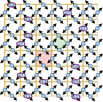
Figure 1: Schematic diagram representing the Kitaev toric code with periodic boundary condition (which is shown by dotted lines in the boundary). The start and plaquette operators, $A_{v}$ and $B_{p}$, are marked in green and pink respectively. Moreover, the clouds represent the local noise which acts on each qubit of the entire state.

As the name suggests, the star operator acts on four qubits situated around a vertex of the lattice while the action of the plaquette operator is again on four qubits on the bond around a plaquette of the 2D lattice. From the definition, all stars and plaquette operators commute with each other. Furthermore, $\hat{A}_{\nu}$s are generators of an Abelian group whose elements can be represented by a loop configuration. In that, all possible trivial loops can be generated by the combination of $\hat{A}_{\nu}$ on each star. An Abelian group Zanardi et al. (2007) comprising of all possible loops helps in identifying the underlying structure of the ground state, i.e., the element of the group is, $a_{\left\{r_{1},r_{2},\ldots,r_{N/2}\right\}}=\hat{A}_{1}^{r_{1}}\cdot\hat{A}_{2}^{r_{2}}\ldots\hat{A}_{\frac{N}{2}-1}^{r_{\frac{N}{2}-1}}$, where ${r_{i}\in{0,1}}$, i.e., the star operator is active on site $i$ or not. The underlying lattice becomes a torus as the periodic boundary conditions are imposed on both the horizontal and vertical edges of the lattice. The torus structure increases the number of ground states to four linearly independent states which satisfy the toric code. In particular, the centres of two non-trivial loops match the centres of the tube and the torus, respectively.

Since Eq. (1) reduces to the analytically solvable Kitaev toric code with some energy shifts, the ground state (GS) properties are already known Kitaev (2006). One of the ground states in the four-dimensional GS manifold can be expressed as  Castelnovo and Chamon (2008)

$$|GS\rangle=\prod_{v}(1+\hat{A}_{v})|0\rangle^{\bigotimes N}.$$ (2)

Here $N$ is the total number of spins and $|0\rangle^{\bigotimes N}$ represents a fully magnetized state with all spins pointing up. Therefore, one can immediately identify Eq. (2) as the ground state of Eq. (1) in the limit $\beta\rightarrow 0$.

In the other extreme limit, i.e., $\beta\rightarrow\infty$, the ground state of Eq. (1) becomes fully magnetized which suggests that the system exhibits a topological quantum phase transition from a topological phase to a magnetized phase as $\beta$ is varied from $\beta=0$ to $\beta\rightarrow\infty$.

The exact ground state of the system can be analytically obtained  Castelnovo and Chamon (2008) as

$$|GS(\beta)\rangle=\frac{1}{\sqrt{Z(\beta)}}\sum_{a\in G}\exp^{\beta\sum_{i}\sigma_{i}^{z}(a)}a|0\rangle,$$ (3)

where $g\in G$ refers to the loop operators from the Abelian group $G$, $Z(\beta)=\sum_{a\in G}\exp^{\frac{\beta}{2}\sum_{i}\sigma_{i}^{z}(a)}$ and $\sigma^{z}_{i}(a)=\mp 1$ depending on if the spin $i$ has an intersection with the loop operator $a$ or not. The static properties of $\hat{H}_{NLTC}(\beta)$ can help us to fix the initial state and the quenching Hamiltonian.

II.2 Quench across the critical point

A sudden change of parameters under evolution, more popularly known as quantum quench or sudden quench turns out to be an important tool to study the non-equilibrium properties of the system under consideration. It has been established that the ground state of the toric code is resilient to local perturbations. We consider a study in which the system is no more under equilibrium but actively undergoes evolution Tsomokos et al. (2009).

To achieve the goal of mimicking equilibrium physics, especially the TQPT from the dynamical state, the initial state is chosen to be the ground state of $H_{NLTC}(\beta_{0})$, i.e., at $t=0$, $|GS\rangle$ is taken as the initial state for dynamics. After the sudden quench in which $\beta_{0}$ is abruptly changed to $\beta_{1}$, the system evolves according to the Hamiltonian $H_{NLTC}(\beta_{1})$. To identify TQPT through evolution, we ensure that $\beta_{0}$ and $\beta_{1}$ are either taken from the same phase or from a different phase Heyl (2018); Heyl et al. (2013). The evolved state takes the form as

$$|\psi(\beta_{0},\beta_{1},t)\rangle=U(\beta_{1},t)|\psi_{0}(\beta_{0})\rangle=e^{-iH_{NLTC}(\beta_{1})t}|\psi_{0}(\beta_{0})\rangle,$$ (4)

where $|\psi_{0}(\beta_{0})\rangle$ is the ground state of the $H_{NLTC}(\beta_{0})$ Hamiltonian. For our investigation, the initial state is chosen with $\beta_{0}\neq 0$ while the post-quenched Hamiltonian is always considered to be the original Kitaev code, i.e., $\beta_{1}=0$.

III Measures used for detecting Criticalities in Evolution

Let us briefly discuss the measures that we use to detect TDQPT.

Loschmidt echo and rate function. First, we employ the conventional DQPT detector, Loschmidt echo Heyl et al. (2013); Heyl (2018) which is computed for distinguishing the equilibrium phases from the dynamical state. It is defined as $\mathcal{L}(t)=|\langle\psi_{t}|\psi_{0}\rangle|^{2}$, where $|\psi_{0}\rangle$ and $|\psi_{t}\rangle$ are the initial and the evolved states respectively. It has been observed that in the case of a quantum transverse Ising chain, the evolved state becomes completely orthogonal with the initial state if the quench is performed to a different phase from the initial one. In order to detect the existence of such zeros, the logarithm of it is introduced, known as the Loschmidt rate, which reads as $\Lambda(t)=\lim_{N\to\infty}\frac{1}{N}{\ln[\mathcal{L}(t)]}=\lim_{N\to\infty}\frac{2}{N}{\ln[\langle\psi_{t}|\psi_{0}\rangle}]$. The non-analytic behavior of the rate function with time is argued to be analogous to the behavior of the free energy in the classical phase transition Heyl (2018) if we replace $i\times t$ in the evolution operator with the inverse temperature in the partition function.

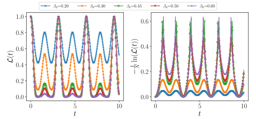
Figure 2: (a) Loschmidt echo (ordinate) of the non-linearly perturbed Kitaev model vs time, t (abscissa) for different choices of parameters for the ground state as initial states, $\beta_{0}$. The sudden quench is performed with the Hamiltonian having $\beta_{1}=0$. The initial and final Hamiltonians are in different phase when $\beta_{0}>\beta_{critical}=0.4407$ while they are in the same phase for $\beta_{0}<\beta_{critical}=0.4407$. (b) Rate function, $\Lambda(t)$, (vertical axis) with respect to time (horizontal axis). The system-size is chosen to be $28$. All the axis are dimensionless.

Specifically, it was shown that uniformly-spaced kinks appear in the time evolution of the rate function for the transverse Ising spin model when the initial Hamiltonian and the quenched Hamiltonian belong to different phases while such kinks are absent if they are chosen from the same phase. Notice, however, that many exceptions to this detection process are also reported Vajna and Dóra (2014); Andraschko and Sirker (2014); Gurarie (2019); Haldar et al. (2020); Nandi et al. (2022). However, as we will illustrate in the next section, both $\mathcal{L}(t)$ and $\Lambda(t)$ are capable to identify TQPT from the dynamics.

Entanglement measures. Let us define two entanglement measures, namely genuine multipartite entanglement measure by exploiting the geometric structure of states Sen (De); Wei and Goldbart (2003); Wei et al. (2005b); Blasone et al. (2008); Orús (2008); Buchholz et al. (2016); Das et al. (2016), and block entanglement which is computed by dividing the entire system into two equal blocks.

Genuine multipartite entanglement. A pure state is genuinely multipartite entangled if it is not separable in any bipartition. Moreover, we know that all separable states form a closed and convex set. It gives rise to the possibility of measuring the entanglement of a given state by calculating the distance between the set of separable states and the given state. By denoting the set of non-genuinely multipartite entangled states as $\Lambda_{G}$, the generalized geometric measure (GGM, quantifying genuine multipartite entanglement content of an arbitrary $N$-party state $|\psi\rangle$, is defined as $\mathcal{G}(|\psi\rangle)=1-\max|\langle\phi\mid\psi\rangle|^{2},\,\,|\phi\rangle\in\Lambda_{G}$. By using Schmidt decomposition of a pure state, it reduces to a simple form as

$$\mathcal{G}(|\psi\rangle)=1-\max\left\{\lambda_{i_{1}\text{ :rest }}^{\max},\lambda_{i_{1}i_{2}\text{ :rest }}^{\max_{1}},\ldots,\lambda_{i_{1}i_{2}\ldots i_{M}:\mathrm{rest}}^{\max}\mid\right.$$

$$i_{1},i_{2},\ldots,i_{M}\left.\in\{1,2,\ldots\frac{N}{2}\};i_{k}\neq i_{l};k,l\in\{1,2,\ldots M\}\right\},$$

where $\lambda^{\max}_{i_{1}i_{2}\ldots i_{M}}$ is the largest eigenvalue of the reduced density matrix, $\rho_{i_{1}i_{2}\ldots i_{M}}$ corresponding to a bipartition $M:rest$. Also, in our case, $N$ is always even since an odd number of spins cannot sit on a torus. Although it may seem that one has to calculate all possible bipartitions and thus it requires to compute maximum eigenvalues of $\sum_{i=1}^{\frac{N}{2}}\dbinom{N}{i}=\frac{1}{2}\times(2^{n}+\dbinom{N}{\frac{N}{2}}-2)$ number of matrices. We will prove that it is not the case in the next section.

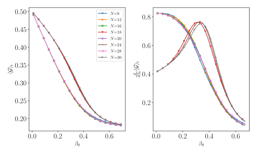
Figure 3: (a) Time-averaged $GGM$, $\langle\mathcal{G}\rangle_{t}$ (ordinate) of the evolved state of $\hat{H}_{NLTC}$ against $\beta_{0}$ (abscissa) for different sizes of $N$. (b) The first derivative of $\langle\mathcal{G}\rangle_{t}$ (y-axis) with respect to $\beta_{0}$ (x-axis). A peak in $\frac{d\langle\mathcal{G}\rangle_{t}}{d\beta_{0}}$ is observed at $\beta_{0}$ close to TQPT. This indicates that the $\langle\mathcal{G}\rangle_{t}$ changes from concave to convex at the transition point. The value of $\beta_{0}$ reaches the exact value of $TQPT$ as $N$ increases. All the axes are dimensionless.

Based on the partial transposition criteria Peres (1996); Horodecki et al. (1996), logarithmic negativity (LN) for an arbitrary state, $\rho_{AB}$, can be defined as Vidal and Werner (2002) $E_{LN}(\rho_{AB})=\log_{2}||\rho_{AB}^{T_{A}}||$, where $||\cdot||$ represents the trace-norm and $\rho_{AB}^{T_{A}}$ denotes the partial transposition of $\rho_{AB}$ with respect to the party $A$ . In the case of pure states, $\rho=|\psi\rangle\langle\psi|$, whose Schmidt-decomposition is written as $|\psi\rangle=\sum_{i}c_{i}|A_{i}\rangle|B_{i}\rangle$, the negativity, $\mathcal{N}(\rho)=\frac{||\rho_{AB}^{T_{A}}||-1}{2}$ reduces to Vidal and Werner (2002) $\mathcal{N}(\rho)=\frac{1}{2}\left[\left(\sum_{\alpha}c_{\alpha}\right)^{2}-1\right]$. By considering the dynamical state, $\rho$ having $N$ parties, we calculate logarithmic negativity by taking bipartition, $N/2:N/2$, which we denote it as $E_{LN}(\rho_{\frac{N}{2}:\frac{N}{2}})$.

IV Detection of Topological Criticalities via Entanglement

To uncover the topological quantum phase transition from the dynamics of the system, we adopt three quantities as defined in the preceding section. We start with the commonly used quantifier for DQPT, Loschmidt echo and rate function.

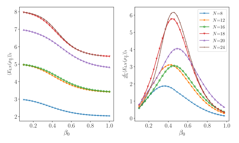
Figure 4: (a) Behavior of time-averaged block logarithmic negativity, $\langle E_{LN}\rangle_{t}$ (ordinate) with respect to $\beta_{0}$ (abscissa) of the modified Kitaev model with various system-sizes, $N$. LN is computed by dividing the $N$-party state into two equal blocks. (b) $\frac{d\langle E_{LN}\rangle_{t}}{d\beta_{0}}$ (y-axis) vs $\beta_{0}$ (x-axis). The peak at $\beta_{0}$ clearly signals topological quantum phase transition occurred at zero temperature. All the axes are dimensionless.

Behavior of Loschmidt echo and kink in rate function. The initial state is the ground state of the Hamiltonian, $\hat{H}_{NLTC}$ with $\beta_{0}<\beta_{critical}$ and also $\beta_{0}>\beta_{critical}$. As mentioned before, the unitary operator involves the Kitaev Hamiltonian, i.e., $\hat{H}_{NLTC}(\beta_{1}=0)$. Hence when $\beta_{0}>\beta_{critical}$, the initial state is in the ground state of a system which is in a paramagnetic phase, thereby belonging to a different phase than the evolving operator while with $\beta_{0}<\beta_{critical}$, both the post- and pre-quenched Hamiltonian belong to the same topologically ordered phase.

We observe that when $\beta_{0}>\beta_{crtical}$, the corresponding Loschmidt echo reaches zero for certain values of $t$ which are equally spaced in $t$ like in the transverse Ising model, as depicted in Fig. 2(a). On the other hand, for $\beta_{0}<\beta_{crtical}$, since the quenched Hamiltonian and the ground state lie in the same phase, $\mathcal{L}(t)$ never vanishes. Therefore, Loschmidt echo, involving both the initial and the dynamical states, clearly recognizes the topological quantum phase transition occurred at zero temperature. As argued before, such behavior becomes more evident when one considers $\Lambda(t)$. Specifically, $\Lambda(t)$ demonstrates a kink exactly at those times when $\mathcal{L}(t)$ vanishes with $\beta_{0}<\beta_{crtical}$ (see Fig. 2 (b)). It clearly signifies that both the quantities are capable to predict TQPT from the dynamical state.

IV.1 Time-averaged Multipartite Entanglement detects Topological Critical Point

Beyond the typical indicator of DQPT, let us demonstrate that entanglement measures, especially multipartite entanglement measures of the evolved state carry the signature of the TQPT (see Haldar et al. (2020) for different spin models). It has already been established that both bipartite and multipartite entanglement of the ground state are capable to detect quantum phase transition in spin Hamiltonian, including topological phase transition considered in this paper (for global entanglement, see Samimi et al. (2022)).

To study the behavior of genuine multipartite entanglement of the evolved state, we compute the time-averaged GGM, denoted by $\langle\mathcal{G}\rangle_{t}$, when the state evolved under the quenched $\hat{H}_{NLTC}(\beta_{1}=0)$ from the ground state of $\hat{H}_{NLTC}(\beta_{0}\neq 0)$ as the initial state. Before presenting the results, let us first establish that the computation of GGM gets simplified by exploiting the characteristics of this model.

Theorem. Eigenvalues from a single-party density matrix of the evolved state only contribute to the maximum involved in GGM.

Proof.

In order to find the eigenvalues in bipartitions, we require to trace out some of the parties, say, $M$. First, notice that the ground state is a superposition of all possible closed loops on the torus. Let us consider the density matrix corresponding to the ground state, given by

$$\hat{\rho}(\beta)=\frac{1}{Z}\sum_{a,a^{\prime}\in G}e^{\frac{\beta}{2}(\hat{\sigma}_{i}^{z}(a)+\hat{\sigma}_{i}^{z}(a^{\prime}))}a|0\ldots 0\rangle\langle 0\ldots 0|a^{\prime},$$ (6)

and the corresponding reduced density matrix of $\{i_{1},i_{2}i_{3}\ldots,i_{M}\}$ parties are obtained by tracing out $M$ parties as

$$\hat{\rho}_{i_{1}i_{2},i_{3}\ldots i_{M}}=\frac{1}{Z}\sum_{\left\{\delta_{k}=0,1\right\}}\sum_{a,a^{\prime}}e^{\frac{\beta}{2}\sum_{i}\left[\hat{\sigma}_{i}^{z}(a)+\hat{\sigma}_{i}^{z}\left(a^{\prime}\right)\right]}$$

$$\times\left\langle\delta_{1}\delta_{2}\ldots\delta_{N-M}|a|0\ldots 0\rangle\langle 0\ldots 0\left|a^{\prime}\right|\delta_{1}\delta_{2}\ldots\delta_{N-M}\right\rangle.$$

As shown in Refs. Samimi et al. (2022); Castelnovo and Chamon (2008), one can prove by contradiction that this state cannot have non-diagonal terms. As described previously, all loops are represented as elements of an Abelian group generated by $A_{\nu}$. In the ground state, each $a_{i}|0\rangle^{\otimes N}$ corresponds to the system configuration of $N$ spins in the $i$-loop configuration. For example, no two closed loops can have one different spin, and hence it is not possible to have

$$\begin{array}[]{l}\left(\left\langle\delta_{1},\delta_{2},\ldots,\delta_{x},\ldots,\delta_{N}\right|\right)\left(a_{1}|0\rangle^{\otimes N}\right)\\ \quad\times\left({}^{N\otimes}\langle 0|a_{2}\right)\left(\left|\delta_{1},\delta_{2},\ldots,\delta_{x}^{\prime},\ldots,\delta_{N}\right\rangle\right)\neq 0,\end{array}$$ (8)

when $x\neq x^{\prime}$. A similar argument can be made for any reduced density matrices for the ground state which is the initial state during evolution.

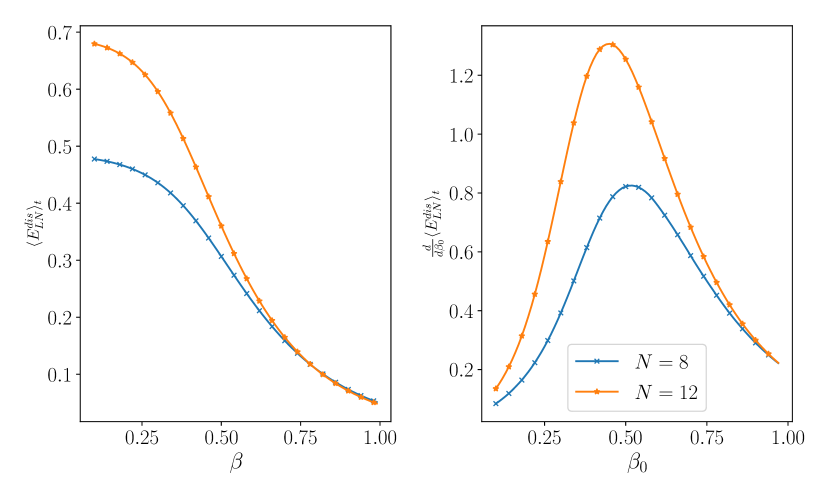
Figure 5: Topological dynamical quantum phase transition under decoherence. The individual qubits of the entire system are in contact with local thermal bath with temperature, $B/T_{E}=10$. (a)Plot of time-averaged LN under repetitive noisy environment, $\langle E_{LN}^{dis}\rangle_{t}$ (ordinate) by varying $\beta_{0}$ (abscissa) of a perturbed Kitaev toric code with different $N$. (b) The first derivative of $\langle E_{LN}^{dis}\rangle_{t}$ (vertical axis) again shows a clear pick at $\beta_{0}$ (horizontal axis) close to critical point. It indicates that even in presence of decoherence, the system clearly carries the information of the phase in the initial Hamiltonian. Both the axes are dimensionless.

Since the evolution operator involves the Kitaev model, the evolved state can be written in the same basis as the ground state and the corresponding local density matrices are again diagonal by using similar logic which are also diagonal in that basis. Moreover, we note that the $M$-party reduced state has eigenvalues $e_{1},\ldots e_{2^{M}}$, written in decreasing order say. It can be easily found that $(M-1)$-party reduced state has $2^{M-1}$ number of eigenvalues of the form $e_{i}+e_{i+1}$ ($i=1,2,\ldots 2^{M}-1$). It clearly shows that the maximum eigenvalue of $(M-1)$-party is bigger than that obtained from the $M$-party state. Hence, the single-site reduced density matrix has the maximum eigenvalue which contributes in the computation of GGM for the evolved state.

∎

Let us now elaborate the way we compute the time-average GGM. Following the quench as described before, we calculate GGM at every time step, and then perform averaging over time, indicated as

$$\langle\mathcal{G}\rangle_{t}=\frac{\sum_{t=t_{i}}^{t_{f}}\mathcal{G}(|\psi(\beta_{0},\beta_{1},t)\rangle}{L},$$ (9)

where $t_{i(f)}$ is the initial (final) time, and $L=\frac{t_{f}-t_{i}}{\delta t}$ with $\delta t$ being the step size. For illustration in Fig. 3, we choose $t_{i}$ and $t_{f}$ as $0$ and $10$ respectively while the step size is taken to be $0.01$. The observations can be summarized as follows.

1. When both the initial and the post-quench Hamiltonian are in the topological phase, the time-averaged GGM is very high, almost close to its maximum value. In other words, the initial state should be prepared as the ground state of the Hamiltonian with a very low $\beta<<\beta_{critical}$ to produce a highly genuine multipartite entangled state during dynamics. Such a behavior can be termed as topological robustness which persists in presence of a weak perturbation, $\beta_{0}$.

2. With the increase of the perturbation of the initial state, $\beta_{0}$, $\langle\mathcal{G}\rangle_{t}$ decreases as shown in Fig. 3 (a). When the initial and the quenched Hamiltonian belong to the different phases, i.e., when the quenching Hamiltonian is in the paramagnetic phase, the time-averaged GGM content is lower than the scenario with both the initial and final Hamiltonians being in the same phase.

3. At the topological phase transition point, $\langle\mathcal{G}\rangle_{t}$ changes its curvature from concave to convex. The derivative of the time-averaged GGM with respect to $\beta_{0}$, i.e., $\frac{d\langle\mathcal{G}\rangle_{t}}{d\beta_{0}}$ shows maximum at $\beta_{critical}$ (see Fig. 3 (b)). However, for certain small system-size, this is not the case and the double derivative of $\langle G\rangle_{t}$ shows the maximum.

The above inspections strongly indicate that genuine multipartite entanglement of the dynamical state can efficiently signal the topological phase transition in equilibrium. Moreover, high multipartite entanglement content identifies the beneficial role of the topologically ordered phase in the deformed Kitaev model and its importance in quantum information processing tasks.

Block entanglement. Let us now examine whether other multipartite entanglement measures are also able to reveal TQPT from the dynamics. Towards that aim, we compute the time-averaged value of LN in $N/2:N/2$ bipartition, i.e., we replace $\mathcal{G}$ by $E_{LN}$ in the definition of $\langle\mathcal{G}\rangle_{t}$ in Eq. (9). For all system-sizes, we observe that $\langle E_{LN}(\rho_{N/2})\rangle_{t}$ in equal bipartition with the variation of $\beta_{0}$ becomes convex to concave and the point of inflexion indicates the topological phase transition at zero temperature which is prominent with the behavior of $\frac{d\langle E_{LN}\rangle_{t}}{d\beta_{0}}$ as shown in Fig. 4 (b).

V Effect of local repetitive interaction on Toric code

Until now, the dynamics that we have studied is unitary which means that the system is isolated and is not interacting with the environment. We have shown that entanglement as well as Loschmidt echo from the evolved state can faithfully signal the topological quantum phase transition present at zero temperature.

We will now ask the following question – can we still predict the topological critical point from dynamics using entanglement, even when the system is in contact with a bath? It is quite reasonable to assume that decoherence may eliminate the information about the equilibrium phase transition carried by a evolved state in unitary dynamics. However, we will manifest that this is not the case.

Let us consider the scenario in which each qubit of the system is repeatedly interacting with a spin-bath at a given thermal equilibrium, having temperature $T$ governed by a Hamiltonian, $H_{B_{i}}=B\hat{\sigma}^{z}_{i}$ Dhahri (2008); Chanda et al. (2018). In our case, the local thermal state interacts with the individual spin on the Toric code. In this scenario, we assume that each bath interacts with the system-spin for a very small period of time, $\delta t$ and the corresponding interacting Hamiltonian, $H_{int}=\sqrt{k/\delta t}(\hat{\sigma}^{x}_{S}\otimes\hat{\sigma}^{x}_{E}+\hat{\sigma}^{y}_{S}\otimes\hat{\sigma}^{y}_{E})$. After the interaction for $\delta t$ period of time, the system-environment entangled state is again reset to be a product state between the system and the environment, thereby ensuring the Markovian dynamics. The evolution is governed by the master equation Ángel Rivas et al. (2014); Breuer and Petruccione (2007); Rivas and Huelga (2012)

$$\frac{d\rho_{S}}{dt}=-\frac{i}{\hbar}\left[H_{S},\rho_{S}\right]+\mathcal{D}\left(\rho_{S}\right),$$ (10)

where $\mathcal{D}$ is the dissipative part dictated by the choice of the environment, and $H_{NLTS}$ is the Hamiltonian of the system, $H_{S}$. The dissipative term in the Markovian limit with the assumption of the weak coupling limit (i.e., we assume that interaction strength is much weaker than the local terms) in this case reduces to

$$\mathcal{D}\left(\rho_{S}\right)=\frac{2k}{\hbar^{2}}\sum_{i=1}^{3}\sum_{l=0}^{1}p_{l}\left[2\eta_{i}^{l+1}\rho_{S}\eta_{i}^{l}-\left\{\eta_{i}^{l}\eta_{i}^{l+1},\rho_{S}\right\}\right],$$ (11)

where $p_{l}=Z_{E}^{-1}\exp\left[\frac{(-1)^{l}B}{T_{E}}\right]$, $Z_{E}=\operatorname{tr}\left[\exp\left(\frac{-H_{E}}{T_{E}}\right)\right]$ with the temperature of the bath Hamiltonian, $B$, being $T_{E}$ and $\eta_{i}^{\alpha}=(\sigma_{i}^{x}+i(-1)^{\alpha}\sigma_{i}^{y})/2$, where the subscript $d_{i}$ denotes the .

The initial state is again chosen to be the ground state of $H_{NLTS}$ with different $\beta_{0}\neq 0$. By solving the above master equation, we obtain $\rho(t)$ at a given time which is used to compute the time-averaged LN by partitioning the entire system into equal blocks. Notice that due to the dissipative term, the evolved state is no more a pure state but a noisy density matrix and hence the computation of GGM via Schmidt coefficients is not possible (see Buchholz et al. (2016); Das et al. (2016)).

For a fixed system-size, $N$, and fixed temperature of the bath (for Fig. 5, $B/T_{E}=10$), we observe that $\langle E_{LN}^{dis}\rangle_{t}$ decreases substantially since all the qubits in the perturbed Kitaev toric code interacts with the thermal bath repeatedly. However, the overall behavior of the time-averaged entanglement remains same which can be seen by comparing Figs. 5 and 4. In particular, we find that when the initial state is prepared in the topologically ordered phase, the dynamical state even in presence of noisy environment can create high entanglement compared to the initial state prepared in the paramagnetic phase.

Moreover, depending on the choice of the phase of the initial state, the curvature of $\langle E_{LN}^{dis}(\rho_{\frac{N}{2}:\frac{N}{2}})\rangle_{t}$ changes to convex at the TQPT point from concave and therefore, $\frac{d\langle E_{LN}^{dis}\rangle_{t}}{dt}$ shows rise at the quantum critical point which is in good agreement with the exact topological phase transition point.

VI Summary

In many-body systems, local order parameters can commonly be employed to characterize quantum phases. The topological order of the system, which is resilient to local disruption, is an exception. It is known that the non-linearly perturbed Kitaev toric code undergoes a quantum phase transition (QPT) from the topological phase to a paramagnetic one by tuning the nonlinear perturbation parameter. The best feature of this model is that the ground state can be found exactly and also exhibits topological order which is robust against local perturbation. There is a constant effort to detect QPT occurring at zero temperature by investigating the evolved state via sudden quench in distinct phases across the quantum critical point.

In summary, we studied the quench dynamics of the non-linearly perturbed Kitaev toric code and searched for the signatures of topological quantum phase transitions in the dynamics which we refer to as topological dynamical quantum phase transition (TDQPT). We choose the initial state for different values of perturbation from both sides of the quantum critical point and quench the system with the original Kitaev code. In addition to the conventional markers of a quantum critical point in the dynamical state, such as the Loschmidt echo and the rate function, we used various entanglement quantifiers, namely time-averaged genuine multipartite entanglement quantified via generalized geometric measure, and block entanglement to detect the TDQPT. We found that under closed unitary dynamics, all the identifiers can distinguish between the instances in which the initial state is in the topological phase or in the paramagnetic phase, thereby signalling the topological QPT. Moreover, we found that the block entanglement in the dynamical state can still identify the topological critical point when all individual qubits of the model are in contact with a thermal bath. The results demonstrate that the topological quantum phase transition is prominent enough to be revealed in dynamics with or without a noisy environment.

References

- Sachdev (2011) S. Sachdev, Quantum Phase Transitions, 2nd ed. (Cambridge University Press, 2011).
- Sengupta et al. (2004) K. Sengupta, S. Powell, and S. Sachdev, Phys. Rev. A 69, 053616 (2004).
- Sen (De) A. Sen(De), U. Sen, and M. Lewenstein, Phys. Rev. A 72, 052319 (2005).
- Heyl (2018) M. Heyl, Reports on Progress in Physics 81, 054001 (2018).
- Heyl et al. (2013) M. Heyl, A. Polkovnikov, and S. Kehrein, Phys. Rev. Lett. 110, 135704 (2013).
- Horodecki et al. (2009) R. Horodecki, P. Horodecki, M. Horodecki, and K. Horodecki, Rev. Mod. Phys. 81, 865 (2009).
- Wei et al. (2005a) T.-C. Wei, D. Das, S. Mukhopadyay, S. Vishveshwara, and P. M. Goldbart, Phys. Rev. A 71, 060305 (2005a).
- Biswas et al. (2014) A. Biswas, R. Prabhu, A. Sen(De), and U. Sen, Phys. Rev. A 90, 032301 (2014).
- Lewenstein et al. (2007) M. Lewenstein, A. Sanpera, V. Ahufinger, B. Damski, A. Sen(De), and U. Sen, Advances in Physics 56, 243 (2007).
- Amico et al. (2008) L. Amico, R. Fazio, A. Osterloh, and V. Vedral, Rev. Mod. Phys. 80, 517 (2008).
- Haldar et al. (2020) S. Haldar, S. Roy, T. Chanda, A. Sen(De), and U. Sen, Phys. Rev. B 101, 224304 (2020).
- Häffner et al. (2008) H. Häffner, C. Roos, and R. Blatt, Physics Reports 469, 155 (2008).
- Duan and Monroe (2010) L.-M. Duan and C. Monroe, Rev. Mod. Phys. 82, 1209 (2010).
- Kaur et al. (2021) K. Kaur, T. Sépulcre, N. Roch, I. Snyman, S. Florens, and S. Bera, Phys. Rev. Lett. 127, 237702 (2021).
- Wen (1995) X.-G. Wen, Advances in Physics 44, 405 (1995), https://doi.org/10.1080/00018739500101566 .
- Wen (2002) X.-G. Wen, Phys. Rev. B 65, 165113 (2002).
- Hamma and Lidar (2008) A. Hamma and D. A. Lidar, Phys. Rev. Lett. 100, 030502 (2008).
- Trebst et al. (2007a) S. Trebst, P. Werner, M. Troyer, K. Shtengel, and C. Nayak, Phys. Rev. Lett. 98, 070602 (2007a).
- Hamma et al. (2008a) A. Hamma, W. Zhang, S. Haas, and D. A. Lidar, Phys. Rev. B 77, 155111 (2008a).
- Dennis et al. (2002a) E. Dennis, A. Kitaev, A. Landahl, and J. Preskill, Journal of Mathematical Physics 43, 4452 (2002a), https://doi.org/10.1063/1.1499754 .
- Kitaev (2003) A. Kitaev, Annals of Physics 303, 2 (2003).
- Kitaev (2006) A. Kitaev, Annals of Physics 321, 2 (2006), january Special Issue.
- Trebst et al. (2007b) S. Trebst, P. Werner, M. Troyer, K. Shtengel, and C. Nayak, Phys. Rev. Lett. 98, 070602 (2007b).
- Castelnovo and Chamon (2008) C. Castelnovo and C. Chamon, Phys. Rev. B 77, 054433 (2008).
- Wu et al. (2012) F. Wu, Y. Deng, and N. Prokof’ev, Phys. Rev. B 85, 195104 (2012).
- Dennis et al. (2002b) E. Dennis, A. Kitaev, A. Landahl, and J. Preskill, Journal of Mathematical Physics 43, 4452 (2002b), https://doi.org/10.1063/1.1499754 .
- Nayak et al. (2008) C. Nayak, S. H. Simon, A. Stern, M. Freedman, and S. Das Sarma, Rev. Mod. Phys. 80, 1083 (2008).
- Levin and Wen (2006) M. Levin and X. G. Wen, Phys. Rev. Lett. 96, 110405 (2006).
- Kitaev and Preskill (2006) A. Kitaev and J. Preskill, Phys. Rev. Lett. 96, 110404 (2006).
- Jiang et al. (2012) H.-C. Jiang, Z. Wang, and L. Balents, Nature Physics 8, 902 (2012).
- Yao and Qi (2010) H. Yao and X.-L. Qi, Phys. Rev. Lett. 105, 080501 (2010).
- Abasto et al. (2008) D. F. Abasto, A. Hamma, and P. Zanardi, Phys. Rev. A 78, 010301 (2008).
- Hamma et al. (2008b) A. Hamma, W. Zhang, S. Haas, and D. A. Lidar, Phys. Rev. B. 77, 155111 (2008b).
- Chen and Li (2010) Y. X. Chen and S. W. Li, Phys. Rev. A 81, 032120 ((2010)).
- Zhang et al. (2022) Y.-R. Zhang, Y. Zeng, T. Liu, H. Fan, J. Q. You, and F. Nori, Phys. Rev. Res. 4, 023144 (2022).
- Schotte et al. (2019) A. Schotte, J. Carrasco, B. Vanhecke, L. Vanderstraeten, J. Haegeman, F. Verstraete, and J. Vidal, Phys. Rev. B 100, 245125 (2019).
- Samimi et al. (2022) E. Samimi, M. H. Zarei, and A. Montakhab, Phys. Rev. A 105, 032438 (2022).
- K. J. and Pal (2022) H. K. J. and A. K. Pal, Phys. Rev. A 105, 052421 (2022).
- Dusuel et al. (2011) S. Dusuel, M. Kamfor, R. Orús, K. P. Schmidt, and J. Vidal, Phys. Rev. Lett. 106, 107203 (2011).
- Zarei (2015) M. H. Zarei, Phys. Rev. A 91, 022319 (2015).
- Zarei (2019) M. H. Zarei, Phys. Rev. B 100, 125159 (2019).
- Vidal et al. (2009) J. Vidal, R. Thomale, K. P. Schmidt, and S. Dusuel, Phys. Rev. B 80, 081104 (2009).
- Sen (De) A. Sen(De) and U. Sen, Phys. Rev. A 81, 012308 (2010).
- Vidal and Werner (2002) G. Vidal and R. F. Werner, Phys. Rev. A 65, 032314 (2002).
- Plenio (2005) M. B. Plenio, Phys. Rev. Lett. 95, 090503 (2005).
- Zanardi et al. (2007) P. Zanardi, L. Campos Venuti, and P. Giorda, Phys. Rev. A 76, 062318 (2007).
- Tsomokos et al. (2009) D. I. Tsomokos, A. Hamma, W. Zhang, S. Haas, and R. Fazio, Phys. Rev. A 80, 060302 (2009).
- Vajna and Dóra (2014) S. Vajna and B. Dóra, Phys. Rev. B 89, 161105 (2014).
- Andraschko and Sirker (2014) F. Andraschko and J. Sirker, Phys. Rev. B 89, 125120 (2014).
- Gurarie (2019) V. Gurarie, Phys. Rev. A 100, 031601 (2019).
- Nandi et al. (2022) P. Nandi, S. Bhattacharyya, and S. Dasgupta, Phys. Rev. Lett. 128, 247201 (2022).
- Wei and Goldbart (2003) T.-C. Wei and P. M. Goldbart, Phys. Rev. A 68, 042307 (2003).
- Wei et al. (2005b) T.-C. Wei, D. Das, S. Mukhopadyay, S. Vishveshwara, and P. M. Goldbart, Phys. Rev. A 71, 060305 (2005b).
- Blasone et al. (2008) M. Blasone, F. Dell’Anno, S. De Siena, and F. Illuminati, Phys. Rev. A 77, 062304 (2008).
- Orús (2008) R. Orús, Phys. Rev. A 78, 062332 (2008).
- Buchholz et al. (2016) L. E. Buchholz, T. Moroder, and O. Gühne, Annalen der Physik 528, 278 (2016), https://arxiv.org/pdf/1412.7471.pdf .
- Das et al. (2016) T. Das, S. S. Roy, S. Bagchi, A. Misra, A. Sen(De), and U. Sen, Phys. Rev. A 94, 022336 (2016).
- Peres (1996) A. Peres, Phys. Rev. Lett. 77, 1413 (1996).
- Horodecki et al. (1996) M. Horodecki, P. Horodecki, and R. Horodecki, Physics Letters A 223, 1 (1996).
- Dhahri (2008) A. Dhahri, Journal of Physics A: Mathematical and Theoretical 41, 275305 (2008).
- Chanda et al. (2018) T. Chanda, T. Das, D. Sadhukhan, A. K. Pal, A. Sen(De), and U. Sen, Phys. Rev. A 97, 062324 (2018).
- Ángel Rivas et al. (2014) Ángel Rivas, S. F. Huelga, and M. B. Plenio, Reports on Progress in Physics 77, 094001 (2014).
- Breuer and Petruccione (2007) H.-P. Breuer and F. Petruccione, The Theory of Open Quantum Systems (Oxford University Press, 2007).
- Rivas and Huelga (2012) A. Rivas and S. F. Huelga, Open Quantum Systems (Springer-Verlag Berlin Heidelberg, 2012).