Robust computation of optimal transport by $\beta$-potential regularization

Abstract

Optimal transport (OT) has become a widely used tool in the machine learning field to measure the discrepancy between probability distributions. For instance, OT is a popular loss function that quantifies the discrepancy between an empirical distribution and a parametric model. Recently, an entropic penalty term and the celebrated Sinkhorn algorithm have been commonly used to approximate the original OT in a computationally efficient way. However, since the Sinkhorn algorithm runs a projection associated with the Kullback-Leibler divergence, it is often vulnerable to outliers. To overcome this problem, we propose regularizing OT with the $\beta$-potential term associated with the so-called $\beta$-divergence, which was developed in robust statistics. Our theoretical analysis reveals that the $\beta$-potential can prevent the mass from being transported to outliers. We experimentally demonstrate that the transport matrix computed with our algorithm helps estimate a probability distribution robustly even in the presence of outliers. In addition, our proposed method can successfully detect outliers from a contaminated dataset.

1 Introduction

Many machine learning problems such as density estimation and generative modeling are often formulated by a discrepancy between probability distributions (Kanamori et al., 2009; Goodfellow et al., 2014). As a common choice, the Kullback-Leibler (KL) divergence (Kullback and Leibler, 1951) has been widely used since minimizing the KL-divergence of an empirical distribution from a parametric model corresponds to maximum likelihood estimation. However, the KL-divergence suffers from some problems. For instance, the KL-divergence of $p$ from $q$ is not well-defined when the support of $p$ is not completely included in the support of $q$. Moreover, the KL-divergence does not satisfy the axioms of metrics in a probability space. On the other hand, optimal transport (OT) (Villani, 2008) does not suffer from these problems. OT does not require any conditions on the support of probability distributions and thus is expected to be more stable than the KL-divergence. Therefore, the divergence estimator is less prone to diverge to infinity. In addition, OT between two distributions is a metric in a probability space and therefore defines a proper distance between histograms and probability measures (Peyré and Cuturi, 2019). Owing to these nice properties, OT has been celebrated with many applications such as image processing (Rabin et al., 2012) and color modifications (Solomon et al., 2015).

However, the ordinary OT suffers from heavy computation. To cope with this problem, one of the common approaches is to regularize the ordinary OT problem with an entropic penalty term (Boltzmann–Shannon entropy (Dessein et al., 2018)) and use the Sinkhorn algorithm (Knopp and Sinkhorn, 1967) to approximate OT (Cuturi, 2013). The entropic penalty makes the objective strictly convex, ensuring the existence of the unique global optimal solution, and the Sinkhorn algorithm projects this global optimal solution onto a set of couplings in terms of the KL-divergence, a divergence associated with the Boltzmann–Shannon entropy (Dessein et al., 2018). Unfortunately, the KL projection in statistical estimation is often not robust in the presence of outliers (Basu et al., 1998). In our pilot study, we experimentally confirmed that the Sinkhorn algorithm is easily affected by outliers (Figure 1). As can be seen in Table 1, the output value of the Sinkhorn algorithm drastically increases even when only a small number of outliers are included in the dataset.

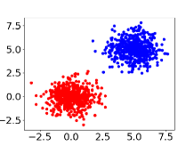
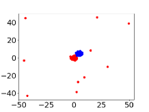
(a) Sets of samples without outliers

(b) Sets of samples with outliers

Figure 1: (a) 500 samples (red) are drawn from $\mathcal{N}([0,0]^{\top},I)$ and 500 samples (blue) are from $\mathcal{N}([5,5]^{\top},I)$. $I$ is the two-dimensional identity matrix. (b) 10 samples from two-dimensional uniform distribution $\mathrm{U}\{(x,y)|-50\leq x,y\leq 50\}$ are added to the red samples.

Table 1: The ouput value of the Sinkhorn algorithm and our algorithm. The exact OT value is 50.13 for the sets of samples in Figure (1).

	Figure 1	Figure 1
The Sinkhorn algorithm	50.74	92.19
Our algorithm	50.10	50.00

The high sensitivity of the Sinkhorn algorithm may lead to undesired solutions in probabilistic modeling when we deal with noisy and adversarial datasets (Kos et al., 2018). Several existing works have tackled this challenge. Staerman et al.(2021) proposed a median-of-means estimator of the $1$-Wasserstein dual to suppress outlier sensitivity. However, the obtained solution is hard to be interpreted as an approximation to OT because the corresponding primal problem is unclear. On the other hand, the following works robustly approximate OT by sending only a small probability mass to outliers, allowing some violation of the coupling constraint: Balaji et al.(2020) used unbalanced OT (Chizat, 2017) with the $\chi^{2}$-divergence as their $f$-divergence penalty on marginal violation to compute OT robustly. This formulation requires access to the outlier proportion, which is usually not available. Moreover, in Section 4.2, we show their method relying on the optimization package CVXPY (Diamond and Boyd, 2016) does not scale to large samples. Mukherjee et al.(2021) mainly focused on outlier detection by truncating the distance matrix in OT. As a downside, one needs to set an appropriate threshold to use their method, which is hardly known in advance. Hence, we still lack a robust OT formulation independent of sensitive hyperparameters, with easily-accessible primal transport matrices.

In this work, we propose to mitigate the outlier sensitivity of the Sinkhorn algorithm by regularizing OT with the $\beta$-potential term instead of the Boltzmann–Shannon entropy. This formulation can be regarded as a projection based on the $\beta$-divergence (Basu et al., 1998; Futami et al., 2018). With some computational tricks, our algorithm is guaranteed not to move any probability mass to outliers (Figure 2). It also suggests that our algorithm computes an approximate OT between the inliers. The approximate OT computed by our method was 50.10 and 50.00 in the settings of Figures 1 and 1, respectively (Table 1), meaning that our method is less prone to be affected by outliers. Through numerical experiments, we demonstrate that our proposed method can measure a distance between datasets more robustly than the Sinkhorn algorithm. As a practical application, we show our proposed method can be applied to an outlier detection task.

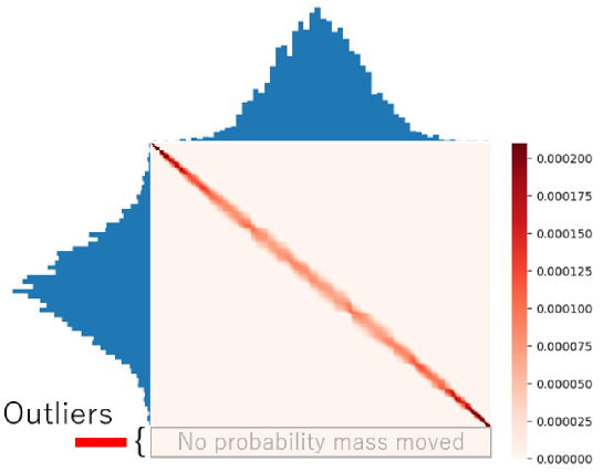
Figure 2: The heatmap of the transport matrix computed with our algorithm. The horizontal histogram is a set of 500 samples from a 1-dimensional standard normal distribution. The vertical histogram is a set of 495 samples from a 1-dimensional standard normal distribution added with 5 outliers with a value of 70. As can be seen from the heatmap, no mass was transported from outliers included in the source histogram.

2 Background

In this section, we first show the formulation of ordinary discrete OT. Subsequently, we review the Bregman divergence. Finally, we introduce the convex regularized discrete OT (CROT) formulation and the alternate Bregman projection to obtain the solution to the CROT.

2.1 Optimal Transport (OT)

We introduce OT in a discrete setting. In this case, OT can be regarded as the cheapest plan to deliver items from $m$ suppliers to $n$ consumers, where each supplier and consumer has supply $\frac{1}{m}$ and demand $\frac{1}{n}$, respectively. In this work, we mainly focus on measuring the transportation cost between two probability distributions. Suppose we have two sets of independent samples $\{\boldsymbol{x}_{i}\}_{i=1}^{m}$ and $\{\boldsymbol{y}_{j}\}_{j=1}^{n}$ drawn from two distributions $P_{x}$ and $P_{y}$, respectively. We write the corresponding empirical measures by $\hat{P}_{x}\coloneqq\frac{1}{m}\sum_{i=1}^{m}\boldsymbol{x}_{i}\delta_{\boldsymbol{x}_{i}}$ and $\hat{P}_{y}\coloneqq\frac{1}{n}\sum_{i=1}^{n}\boldsymbol{y}_{i}\delta_{\boldsymbol{y}_{i}}$, where $\delta_{\boldsymbol{x}}$ is the delta function at position $\boldsymbol{x}$. Let $\boldsymbol{\gamma}\in\mathbb{R}_{+}^{m\times n}$ be the distance matrix, where $\gamma_{ij}$ denotes the distance between $\boldsymbol{x}_{i}$ and $\boldsymbol{y}_{j}$. Transport matrices are confined to

$$\left\{\boldsymbol{\Pi}\in\mathbb{R}^{m\times n}_{+}\,\middle|\,\boldsymbol{\Pi}\boldsymbol{1}_{n}=\frac{\boldsymbol{1}_{m}}{m},\boldsymbol{\Pi}^{\top}\boldsymbol{1}_{m}=\frac{\boldsymbol{1}_{n}}{n}\right\}\eqqcolon\mathcal{G}\left(\frac{\boldsymbol{1}_{m}}{m},\frac{\boldsymbol{1}_{n}}{n}\right),$$ (1)

where $\mathbb{R}^{m\times n}_{+}$ is the set of non-negative reals. We call $\mathcal{G}(\frac{\boldsymbol{1}_{m}}{m},\frac{\boldsymbol{1}_{n}}{n})$ the coupling constraint. In order to keep the notation concise, the Frobenius inner product between two matrices $\boldsymbol{\pi},\boldsymbol{\gamma}\in\mathbb{R}_{+}^{m\times n}$ is denoted by

$$\langle\boldsymbol{\pi},\boldsymbol{\gamma}\rangle\coloneqq\sum_{i,j}\pi_{ij}\gamma_{ij}.$$ (2)

Then, OT between the two empirical distributions $\hat{P}_{x}$ and $\hat{P}_{y}$ is defined as follows (Peyré and Cuturi, 2019):

$$\mathrm{OT}(\hat{P}_{x}\|\hat{P}_{y}) \coloneqq \min_{\boldsymbol{\pi}\in\mathcal{G}(\frac{\boldsymbol{1}_{m}}{m},\frac{\boldsymbol{1}_{n}}{n})}\langle\boldsymbol{\pi},\boldsymbol{\gamma}\rangle.$$ (3)

2.2 Bregman divergence

Let $\mathcal{E}$ be a Euclidean space with inner product $\langle\cdot,\cdot\rangle$ and induced norm $\|\cdot\|$. Let $\phi:\mathcal{E}\to\mathbb{R}$ be a strictly convex function on $\mathcal{E}$ that is differentiable on $\mathrm{int}(\operatorname{dom}\phi)\neq\emptyset$. The Bregman divergence generated by $\phi$ is defined as follows:

$$B_{\phi}(\boldsymbol{x}\|\boldsymbol{y}):=\phi(\boldsymbol{x})-\phi(\boldsymbol{y})-\langle\boldsymbol{x}-\boldsymbol{y},\nabla\phi(\boldsymbol{y})\rangle,$$ (4)

for all $\boldsymbol{x}\in\operatorname{dom}\phi$ and $\boldsymbol{y}\in\operatorname{dom}\phi$. In this paper, for the sake of simplicity, we consider the so-called separable Bregman divergences (Dessein et al., 2018) over the set of transport matrices $\mathcal{G}\left(\frac{\boldsymbol{1}_{m}}{m},\frac{\boldsymbol{1}_{n}}{n}\right)$, which can be decomposed as the element-wise summation:

$$B_{\phi}(\boldsymbol{\pi}\|\boldsymbol{\xi}) = \sum_{i=1}^{m}\sum_{j=1}^{n}B_{\phi}(\pi_{ij}\|\xi_{ij}),$$ (5)

$$\phi(\boldsymbol{\pi}) = \sum_{i=1}^{m}\sum_{j=1}^{n}\phi(\pi_{ij}),$$ (6)

where we used $\phi:\mathbb{R}\to\mathbb{R}$ to denote the generator function same across all elements, with a slight abuse of notation. Suppose now that $\phi$ is of the Legendre type (Bauschke and Borwein, 1997), and let $\mathcal{C}\subseteq\mathcal{E}$ be a closed convex set such that $\mathcal{C}\cap\mathrm{int}(\operatorname{dom}\phi)\neq\emptyset$. Then, for any point $\boldsymbol{y}\in\mathrm{int}(\operatorname{dom}\phi)$, the following problem,

$$T_{\mathcal{C}}(\boldsymbol{y})=\operatornamewithlimits{argmin}_{\boldsymbol{x}\in\mathcal{C}}B_{\phi}(\boldsymbol{x}\|\boldsymbol{y}),$$ (7)

has a unique solution. $T_{\mathcal{C}}(\boldsymbol{y})$ is called the Bregman projection of $\boldsymbol{y}$ onto $\mathcal{C}$ (Dessein et al., 2018).

2.3 Formulation of CROT

Regularization term	dom $\phi$	dom $\psi$
$\beta$-potential ($\beta>1$)	$\mathbb{R}_{+}$	$(\frac{1}{1-\beta},\infty)$
Boltzman-Shannon entropy	$\mathbb{R}_{+}$	$\mathbb{R}$

Table 2: Domains of each regularizer and its Fenchel conjugate.

Here, we give the formulation of the CROT and show that obtaining the optimal solution of the CROT corresponds to minimizing the Bregman divergence between two matrices.

The CROT is formulated as a regularized version of (3) by $\phi$ as follows:

$$L_{\phi}(\boldsymbol{\pi})\coloneqq\min_{\boldsymbol{\pi}\in\mathcal{G}(\frac{\boldsymbol{1}_{m}}{m},\frac{\boldsymbol{1}_{n}}{n})}\langle\boldsymbol{\pi},\boldsymbol{\gamma}\rangle+\lambda\phi(\boldsymbol{\pi}),$$ (8)

where $\lambda>0$ is a regularization parameter. Subsequently, we often work on the dual variable of $\boldsymbol{\pi}$. The dual variable $\boldsymbol{\theta}$ satisfies the following conditions:

$$\boldsymbol{\pi} = \nabla\psi(\boldsymbol{\theta}),$$ (9)

$$\boldsymbol{\theta} = \nabla\phi(\boldsymbol{\pi}),$$ (10)

where $\psi$ is the Fenchel conjugate of $\phi$ (Dessein et al., 2018). The optimal solution of (8) can be understood via the Bregman projection. Let us consider the unconstrained version of (8):

$$\min_{\boldsymbol{\pi}\in\mathbb{R}^{m\times n}}\langle\boldsymbol{\pi},\boldsymbol{\gamma}\rangle+\lambda\phi(\boldsymbol{\pi}).$$ (11)

Since $\langle\boldsymbol{\pi},\boldsymbol{\gamma}\rangle$ is linear and $\phi$ is strictly convex with respect to $\boldsymbol{\pi}$, there is a unique optimal solution $\boldsymbol{\xi}$ for (11):

$$\boldsymbol{\xi}=\nabla\psi(-\boldsymbol{\gamma}/\lambda),$$ (12)

which can be obtained by solving the first-order optimality condition of (11) with the dual relationship $(\nabla\phi)^{-1}=\nabla\psi$:

$$\boldsymbol{\gamma}+\lambda\nabla\phi(\boldsymbol{\xi})=0.$$ (13)

Then,

$$\boldsymbol{\pi}_{\lambda}^{*} \coloneqq\operatornamewithlimits{argmin}_{\boldsymbol{\pi}\in\mathcal{G}(\frac{\boldsymbol{1}_{m}}{m},\frac{\boldsymbol{1}_{n}}{n})}L_{\phi}(\boldsymbol{\pi})$$ (14)

$$=\operatornamewithlimits{argmin}_{\boldsymbol{\pi}\in\mathcal{G}(\frac{\boldsymbol{1}_{m}}{m},\frac{\boldsymbol{1}_{n}}{n})}B_{\phi}(\boldsymbol{\pi}\|\boldsymbol{\xi}),$$ (15)

where the last equality is due to the following equation:

$$\langle\boldsymbol{\pi},\boldsymbol{\gamma}\rangle+\lambda\phi(\boldsymbol{\pi})-\lambda\phi(\boldsymbol{\xi})-\langle\boldsymbol{\xi},\boldsymbol{\gamma}\rangle=\lambda B_{\phi}(\boldsymbol{\pi}\|\boldsymbol{\xi}).$$ (16)

Therefore, the solution of (8) can be interpreted as the Bregman projection of the unconstrained solution $\boldsymbol{\xi}$ onto $\mathcal{G}(\frac{\boldsymbol{1}_{m}}{m},\frac{\boldsymbol{1}_{n}}{n})$. The Sinkhorn algorithm can be used to obtain a solution to OT regularized with the negative of Boltzmann–Shannon entropy $\phi(\pi)=\pi\log\pi-\pi+1$ (Table 5), and runs a projection associated with the KL-divergence where $B_{\phi}(\pi\|\xi)=\pi\log\frac{\pi}{\xi}-\pi+\xi$.

2.4 Alternate Bregman projection

Here, we demonstrate how the Bregman projection onto $\mathcal{G}(\frac{\boldsymbol{1}_{m}}{m},\frac{\boldsymbol{1}_{n}}{n})$ is executed based on Dessein et al.[2018].

Let $\mathcal{C}_{0},\mathcal{C}_{1},\mathcal{C}_{2}$ be the following convex sets:

$$\mathcal{C}_{0} = \mathbb{R}_{+}^{m\times n},$$ (17)

$$\mathcal{C}_{1} = \left\{\boldsymbol{\pi}\in\mathbb{R}^{m\times n}\,\middle|\,\boldsymbol{\pi}\boldsymbol{1}_{n}=\textstyle{\frac{\boldsymbol{1}_{m}}{m}}\right\},$$ (18)

$$\mathcal{C}_{2} = \left\{\boldsymbol{\pi}\in\mathbb{R}^{m\times n}\,\middle|\,\boldsymbol{\pi}^{\top}\boldsymbol{1}_{m}=\textstyle{\frac{\boldsymbol{1}_{n}}{n}}\right\}.$$ (19)

Then, $\mathcal{G}(\frac{\boldsymbol{1}_{m}}{m},\frac{\boldsymbol{1}_{n}}{n})$ can be written as follows:

$$\mathcal{G}(\textstyle{\frac{\boldsymbol{1}_{m}}{m}},\textstyle{\frac{\boldsymbol{1}_{n}}{n}})=\mathcal{C}_{0}\cap\mathcal{C}_{1}\cap\mathcal{C}_{2}.$$ (20)

We can get the Bregman projection onto $\mathcal{G}(\frac{\boldsymbol{1}_{m}}{m},\frac{\boldsymbol{1}_{n}}{n})$ by alternately performing projections onto $\mathcal{C}_{0}$, $\mathcal{C}_{1}$, and $\mathcal{C}_{2}$.

Next, let us consider the projection of a given matrix $\overline{\boldsymbol{\pi}}\in\mathrm{int}(\operatorname{dom}\phi)$ onto $\mathcal{C}_{0}$, $\mathcal{C}_{1}$, and $\mathcal{C}_{2}$. The corresponding projection onto each set is denoted by $\boldsymbol{\pi}_{0}^{*}$, $\boldsymbol{\pi}_{1}^{*}$, and $\boldsymbol{\pi}_{2}^{*}$, respectively. Subsequently, we show how to obtain them (Dessein et al., 2018) (see Section A in the supplementary file for details).

2.4.1 Projection onto $\mathcal{C}_{0}$

When considering the separable Bregman divergence, the projection onto $\mathcal{C}_{0}$ can be performed with a closed-form expression in terms of primal parameters:

$$\pi^{*}_{0,ij}=\max\{0,\overline{\pi}_{ij}\},$$ (21)

where, $\pi^{*}_{0,ij}$ is the $(i,j)$-element of matrix $\boldsymbol{\pi}_{0}^{*}$. Since $\phi^{\prime}$ is increasing, this is equivalently expressed in terms of the dual parameters of $\boldsymbol{\pi}_{0}^{*}$, $\boldsymbol{\theta}_{0}^{*}$, as

$$\theta_{0,ij}^{*}=\max\{\phi^{\prime}(0),\overline{\theta}_{ij}\}.$$ (22)

Here, the dual coordinate of the input matrix $\overline{\boldsymbol{\pi}}$ is denoted by $\overline{\boldsymbol{\theta}}=\nabla\psi(\overline{\boldsymbol{\pi}})$.

2.4.2 Projections onto $\mathcal{C}_{1}$ and $\mathcal{C}_{2}$

Next, we consider the Bregman projection onto $\mathcal{C}_{1}$. The projection onto $\mathcal{C}_{2}$ can be executed in the same way and thus omitted here. The Lagrangian associated to the Bregman projection $\boldsymbol{\pi}_{1}^{*}$ of a given matrix $\overline{\boldsymbol{\pi}}\in\mathrm{int}(\operatorname{dom}\phi)$ onto $\mathcal{C}_{1}$ is given as follows:

$$\mathcal{L}_{1}(\boldsymbol{\pi},\boldsymbol{\mu})=\phi(\boldsymbol{\pi})-\langle\boldsymbol{\pi}, \nabla\phi(\overline{\boldsymbol{\pi}})\rangle+\boldsymbol{\mu}^{\top}(\boldsymbol{\pi}\boldsymbol{1}_{n}-\textstyle{\frac{\boldsymbol{1}_{m}}{m}}),$$

where $\boldsymbol{\mu}\in\mathbb{R}^{m}$ are Lagrange multipliers. Their gradients are given on $\mathrm{int}(\operatorname{dom}\phi)$ by

$$\nabla_{\boldsymbol{\pi}}\mathcal{L}_{1}(\boldsymbol{\pi},\boldsymbol{\mu})=\nabla_{\boldsymbol{\pi}}\phi(\boldsymbol{\pi})-\nabla_{\boldsymbol{\pi}}\phi(\overline{\boldsymbol{\pi}})+\boldsymbol{\mu}{\boldsymbol{1}_{n}}^{\top},$$ (23)

and by noting $(\nabla\phi)^{-1}=\nabla\psi$, $\nabla_{\boldsymbol{\pi}}\mathcal{L}_{1}(\boldsymbol{\pi}_{1},\boldsymbol{\mu})=\boldsymbol{0}_{m\times n}$ if and only if (Dessein et al., 2018),

$$\boldsymbol{\pi}_{1}^{*}=\nabla\psi(\nabla\phi(\overline{\boldsymbol{\pi}})-\boldsymbol{\mu}{\boldsymbol{1}_{n}}^{\top}).$$ (24)

By multiplying $\boldsymbol{1}_{n}$ on the both sides of (24), the following equation system is obtained:

$$\nabla\psi(\nabla\phi(\overline{\boldsymbol{\pi}})-\boldsymbol{\mu}{\boldsymbol{1}_{n}}^{\top})\boldsymbol{1}_{n}=\textstyle{\frac{\boldsymbol{1}_{m}}{m}}.$$ (25)

Due to the separability, the projection onto $\mathcal{C}_{1}$ can be divided into $m$ subproblems in each coordinate of the dual variable as follows:

$$\sum_{j=1}^{n}\psi^{\prime}(\overline{\theta}_{ij}-\mu_{i})=\frac{1}{m}.$$ (26)

To solve equation (26) with respect to $\mu_{i}$, we use the Newton–Raphson method (Akram and ul Ann, 2015).

Algorithm 1 Non-negative alternate scaling algorithm for $\beta$-divergence when $\beta>1$

1:  $\tilde{\boldsymbol{\theta}}\leftarrow-\boldsymbol{\gamma}/\lambda$

2:   $\boldsymbol{\theta^{*}}\leftarrow\max\{\nabla\phi(\boldsymbol{0}_{m\times n}),\tilde{\boldsymbol{\theta}}\}$

3:  for $t$ = 1, 2, …, $T$ do

4:      $\boldsymbol{\tau}=\frac{\nabla\psi(\boldsymbol{\theta^{*}})\boldsymbol{1}_{n}-\frac{\boldsymbol{1}_{m}}{\mathit{m}}}{\nabla^{2}\psi(\boldsymbol{\theta}^{*})\boldsymbol{1}_{n}}$

5:      $\boldsymbol{\tau}\leftarrow\max(\boldsymbol{\tau},\ \hat{\boldsymbol{\theta}}^{*}-\nabla\phi(\frac{\boldsymbol{1}_{m}}{m}))$

6:      $\boldsymbol{\tilde{\theta}}\leftarrow\boldsymbol{\tilde{\theta}}-\boldsymbol{\tau}{\boldsymbol{1}_{n}}^{\top}$

7:      $\boldsymbol{\theta^{*}}\leftarrow\max\{\nabla\phi(\bf{0}),\boldsymbol{\tilde{\theta}}\}$

8:      $\boldsymbol{\sigma}=\frac{{\boldsymbol{1}_{m}}^{\top}\nabla\psi(\boldsymbol{\theta^{*}})-(\frac{\boldsymbol{1}_{n}}{\mathit{n}})^{\top}}{{\boldsymbol{1}_{m}}^{\top}\nabla^{2}\psi(\boldsymbol{\theta}^{*})}$

9:      $\boldsymbol{\sigma}\leftarrow\max(\boldsymbol{\sigma},\hat{\boldsymbol{\theta}}^{*}-\nabla\phi(\frac{\boldsymbol{1}_{n}}{\mathit{n}}))$

10:      $\boldsymbol{\tilde{\theta}}\leftarrow\boldsymbol{\tilde{\theta}}-\boldsymbol{1}_{m}\boldsymbol{\sigma}$

11:      $\boldsymbol{\theta^{*}}\leftarrow\max\{\nabla\phi(\boldsymbol{0}_{m\times n}),\boldsymbol{\tilde{\theta}}\}$

12:  end for

13:  $\boldsymbol{\pi^{*}\leftarrow\nabla\psi(\theta^{*})}$

3 Outlier-robust CROT

In this section, we first formalize a model of outliers. To make the CROT robust against outliers under the model, we propose the CROT with the $\beta$-potential ($\beta>1$) and introduce how to compute the CROT with the $\beta$-potential. Finally, we show its theoretical properties.

3.1 Definition of outliers

In this paper, outliers are formally defined as follows. Suppose we have two datasets $\{\boldsymbol{x}_{i}\}_{i=1}^{m}$ and $\{\boldsymbol{y}_{j}\}_{j=1}^{n}$. We assume $\{\boldsymbol{x}_{i}\}_{i=1}^{m}$ are samples from a clean distribution, while $\{\boldsymbol{y}_{j}\}_{j=1}^{n}$ are samples that are contaminated by outliers. Let $\boldsymbol{\gamma}$ be the distance matrix.

Definition 1.

For $z>0$, the indices of outliers $J$ are defined as follows:

$$\forall j\in J,\ \forall i\in\{1,\ldots,m\},\gamma_{ij}\geq z.$$ (27)

This means that any point in $\{\boldsymbol{y}_{j}\}_{j=1}^{n}$ that is more than or equal to $z$ away from any point in $\{\boldsymbol{x}_{i}\}_{i=1}^{m}$ is considered as outliers.

3.2 $\beta$-potential regularization

We use the $\beta$-potential

$$\phi(\pi)=\frac{1}{\beta(\beta-1)}(\pi^{\beta}-\beta\pi+\beta-1),$$ (28)

associated with the $\beta$-divergence,

$$B_{\phi}(\pi\|\xi)=\frac{1}{\beta(\beta-1)}(\pi^{\beta}+(\beta-1)\xi^{\beta}-\beta\pi\xi^{\beta-1}),$$ (29)

to robustify the CROT, where $\beta>1$. The domains of primal $\phi$ and its Fenchel conjugate $\psi$ are shown in Table 5.

Our proposed algorithm is shown in Algorithm 1. The dual coordinate of the unconstrained CROT solution is denoted by $\boldsymbol{\tilde{\theta}}=\nabla\phi(\boldsymbol{\xi})$. We execute the projections in the cyclic order of $\mathcal{C}_{0}\rightarrow\mathcal{C}_{1}\rightarrow\mathcal{C}_{0}\rightarrow\mathcal{C}_{2}\rightarrow\mathcal{C}_{0}\rightarrow\mathcal{C}_{1}\rightarrow\mathcal{C}_{0}\rightarrow\mathcal{C}_{2}\rightarrow\cdots$.

Lines 2, 7, and 11 in Algorithm 1 enforce the dual constraint $\theta_{ij}^{*}\geq\frac{1}{1-\beta}$ corresponding to $\operatorname{dom}\psi=(\frac{1}{1-\beta},\infty)$ (Table 5). Lines 4–6 correspond to the projection onto $\mathcal{C}_{1}$ implemented on the dual coordinate. Since the dual variable must satisfy $\theta_{ij}^{*}\geq\frac{1}{1-\beta}$ due to $\operatorname{dom}\psi=(\frac{1}{1-\beta},\infty)$, we update the dual variable only once in the Newton–Raphson method (line 4) since $\theta_{ij}^{*}\geq\frac{1}{1-\beta}$ is no longer guaranteed after the first update. Similarily, the projection onto $\mathcal{C}_{2}$ is shown in lines 8–10.

The procedure in line 5 is based on Section 4.6 in Dessein et al.(2018) accelerating the convergence of Algorithm 1 by truncating the optimization variable $\boldsymbol{\tau}$, which we describe subsequently. Recall that, for any $i$, we have the following condition,

$$\forall j,\ 0\leq\pi_{1,ij}^{*}\leq\textstyle{\frac{1}{m}},$$ (30)

implicitly from the coupling constraint (1). Since naively updating Newton–Raphson method can “overshoot”, we truncate $\boldsymbol{\tau}$ so that (30) is satisfied after each update. Below, we show this condition is satisfied mathematically. Let $\hat{\boldsymbol{\theta}}^{*}$ be the $m$-dimensional vector whose $i$th element is the largest value in the $i$th row of $\boldsymbol{\theta}^{*}$ defined as follows:

$$\hat{\theta}^{*}_{i} := \mathrm{max}\{\theta^{*}_{ij}\}_{1\leq j\leq n}.$$ (31)

Since $\phi$ is convex,

$$0\leq\pi_{1,ij}^{*}\leq\frac{1}{m}$$

$$\iff \phi^{\prime}(0)\leq\phi^{\prime}(\pi_{1,ij}^{*})=\theta^{*}_{1,ij}\leq\phi^{\prime}(\frac{1}{m})$$ (32)

holds. Hence, for every $i$, if we lower-bound $\tau_{i}$, the Newton–Raphson decrement for the $i$th row of $\boldsymbol{\theta^{*}}$ as

$$\tau_{i} \leftarrow \max\{\tau_{i},\hat{\theta}^{*}_{i}-\phi^{\prime}\left(\textstyle{\frac{1}{m}}\right)\},$$ (33)

then, for any $j$,

$$\tilde{\theta}_{ij}-\tau_{i} \leq \theta^{*}_{ij}-\tau_{i}$$ (34)

$$\leq \hat{\theta}^{*}_{i}-\tau_{i}$$ (35)

$$\leq \phi^{\prime}\left(\textstyle{\frac{1}{m}}\right).$$ (36)

This means that every element in the $i$th row of $\tilde{\boldsymbol{\theta}}$ computed in line 6 in Algorithm 1 is no larger than $\phi^{\prime}(\frac{1}{m})$. After line 7, $\boldsymbol{\theta}^{*}$ satisfies the condition (30). Similarly, we force $\pi_{2,ij}$ to satisfy the following conditions:

$$\forall i,\ 0\leq\pi_{2,ij}\leq\textstyle{\frac{1}{n}}.$$ (37)

After line 11, this condition is satisfied.

3.3 Theoretical analysis

In the presence of outliers, we expect to approximate the OT by preventing mass transport to outliers. This property is formalized below.

Definition 2.

Suppose $\boldsymbol{\pi}\in\mathbb{R}_{+}^{m\times n}$ and a set of indices O $\subseteq\{1,\ldots,n\}$ satisfies the following condition:

$$\forall i,\pi_{ij}=0\ \ \mathrm{if}\ \ j\in O.$$ (38)

Then, we say $\boldsymbol{\pi}$ transports no mass to O.

Although we do not expect to transport any mass to outliers, the optimal solution of the CROT must satisfy the coupling constraint and then the condition (38) is never satisfied. To ensure (38), we consider solving the CROT with only a finite number of updates subsequently. Then, an intermediate solution can satisfy (38), although the coupling constraint is not satisfied. This is in stark contrast to the previous works (Chizat, 2017; Balaji et al., 2020), which cannot avoid transporting some mass to outliers.

The following proposition provides sufficient conditions on the number of iterations $T$ to ensure the condition (38). Refer to Section B in the supplementary file for the proof.

Proposition 1.

For a given $z\ (>\frac{\lambda}{\beta-1})$, let $J\subseteq\{1,\ldots,n\}$ be a subset of indices which satisfies the condition shown in Definition 1. Suppose we obtained a transport matrix $\boldsymbol{\pi}^{\mathrm{output}}$ by running the alogrithm $T$ times satisfying the following condition:

$$T<\frac{\frac{z}{\lambda}(\beta-1)-1}{(\frac{1}{m})^{\beta-1}+(\frac{1}{n})^{\beta-1}}.$$ (39)

Then, $\boldsymbol{\pi}^{\mathrm{output}}$ transports no mass to J.

Here, $z>\frac{\lambda}{\beta-1}$ is necessary so that $T$ is upper-bounded by a positive number. Intuitively, this means that the transport matrix obtained by Algorithm 1 disregards points distant from inliers more than or equal to $z$. Note that the condition (68) tells us that a sufficiently small number of iterations $T$ leads to an approximate CROT solution that does not transport any mass to outliers.

We discuss the selection of hyperparameters $\beta$ and $\lambda$ in Sections 4.3.

4 Experiments

Here, we show two applications of our method to demonstrate the practical effectiveness. In both of the experiments in Sections 4.1 and 4.2, we set the hyperparameters in the proposed method as $\beta=1.2$ and $\lambda=2$. We discuss the selection of these hyperparameters in Section 4.3.

4.1 Measuring distance between datasets

In the first experiments, we numerically confirm that our method can compute the distance more robustly than the Sinkhorn algorithm. We used the following benchmark datasets: MNIST (Deng, 2012), FashionMNIST (Xiao et al., 2017), KMNIST (Clanuwat et al., 2018), and EMNIST(Letters)(Cohen et al., 2017). From each benchmark dataset, we randomly sampled 10000 data points, and split them into two subsets, each containing 5000 data. We regarded these data points as inliers. Then a portion of one subset was replaced by data from another benchmark dataset which were regarded as outliers. We computed CROT and outlier-robust CROT between these two subsets, and investigated how they changed when the outlier ratio are 5%, 10 %, 15%, 20%, 25% and 30%. We simply used the raw data to compute the distance matrix $\gamma_{ij}=\|\boldsymbol{x}_{i}-\boldsymbol{y}_{j}\|_{2}^{2}$, i.e., the Euclidean distance between raw data, and used their median value as the threshold $z$. In this way, we expect that outliers are distinguished from inliers. The results are shown in Figure 3. Although the distance computed by the Sinkhorn algorithm drastically changes when the outlier ratio gets larger, the degree of change in the output values of our algorithm is milder in every dataset. Therefore, we can see that our algorithm computes the distance between datasets more stably than the Sinkhorn algorithm.

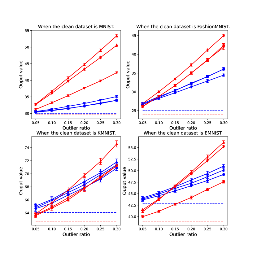
Figure 3: The mean and standard deviation of the output value of the Sinkhorn algorithm (red) and our algorithm (blue) over 20 runs. $\bigcirc$, $\triangle$, $\triangledown$, and $\diamondsuit$ represents when the outlier dataset are MNIST, FashionMNIST, KMNIST, and EMNIST, respectively. The dotted line is the output value when the dataset is clean.

4.2 Applications to outlier detection

	Outliers	Inliers
One-class SVM	49.78 $\pm$ 1.83 %	49.99 $\pm$ 0.10 %
Local outlier factor	49.43 $\pm$ 3.68 %	99.13 $\pm$ 0.11 %
Isolation forest	42.78 $\pm$ 6.95 %	72.81 $\pm$ 3.34 %
Elliptical envelope	95.57 $\pm$ 2.77 %	69.37 $\pm$ 5.61 %
Baseline technique (95th)	92.78 $\pm$ 1.67 %	92.66 $\pm$ 0.44 %
Baseline technique (97.5th)	84.19 $\pm$ 2.10 %	96.41 $\pm$ 0.32 %
Baseline technique (99th)	65.04 $\pm$ 2.75 %	98.60 $\pm$ 0.16 %
ROBOT (95th)	99.96 $\pm$ 0.08 %	68.76 $\pm$ 0.49 %
ROBOT (97.5th)	99.89 $\pm$ 0.14 %	77.22 $\pm$ 0.63 %
ROBOT (99th)	99.48 $\pm$ 0.31 %	84.79 $\pm$ 0.47 %
Our Method (95th)	98.98 $\pm$ 0.66 %	86.72 $\pm$ 0.72 %
Our Method (97.5th)	96.96 $\pm$ 1.71 %	91.58 $\pm$ 0.38 %
Our Method (99th)	92.25 $\pm$ 1.53 %	95.73 $\pm$ 0.34 %

Table 3: The percentage of true outliers/inliers detected as outliers/inliers over 50 runs. The numbers show the mean and standard deviation. “(Xth)” means $X$th percentile was used in its subsampling phase.

Our algorithm enables us to detect outliers. Let $\mu_{m}$ be a clean dataset and $\nu_{n}$ be a dataset which is polluted with outliers. We regard the $j$th data point in $\nu_{n}$ is an outlier if Algorithm 1 outputs a transport matrix whose $j$th column is all zeros.

In this experiment, we used Fashion-MNIST (Xiao et al., 2017) as a clean dataset and MNIST (Deng, 2012) as outliers. $\nu_{n}$ consists of 9500 images from Fashion-MNIST and 500 images from MNIST. $\mu_{m}$ consists of 10000 images from Fashion-MNIST. We computed the transport matrix with the two datasets and identified the outlying MNIST images. We simply used the raw data to compute the distance matrix $\gamma_{ij}=\|\boldsymbol{x}_{i}-\boldsymbol{y}_{j}\|^{2}_{2}$, i.e., the Euclidean distance between raw data.

We compared the proposed method with the “ROBust Optimal Transport” (ROBOT) method (Mukherjee et al., 2021) and the method proposed by Balaji et al.(2020) , which are existing methods to compute OT robustly. We also compared our method with a variety of popular outlier detection algorithms available in scikit-learn (Pedregosa et al., 2011): the one-class support vector machine (SVM) (Schölkopf et al., 1999), local outlier factor (Breunig et al., 2000), isolation forest (Liu et al., 2008), and elliptical envelope (Rousseeuw and van Driessen, 1999). In the ROBOT method, we set the cost truncation hyperparameter to the (1) 95th (2) 97.5th (3) 99th percentile of the distance matrix in the subsampling phase (Mukherjee et al., 2021).

For our method, the distance tolerance parameter $z$ in Definition 1 is necessary to detect outliers by leveraging Proposition 2. Once $z$ is chosen, after running the algorithm $\left\lfloor\frac{\frac{z}{\lambda}(\beta-1)-1}{(\frac{1}{m})^{\beta-1}+(\frac{1}{n})^{\beta-1}}\right\rfloor$ times satisfying the condition (68), points in $\nu_{n}$ that are far from any points in $\mu_{m}$ with more than or equal to distance $z$ are regarded as outliers. To determine $z$, we need a subsampling phase using the clean dataset similar to Mukherjee et al.(2021). We propose the following heuristics: since we know that $\mu_{m}$ is clean, we subsample two datasets from it and compute the distance matrix. Then, we choose the minimum value for each row and use the largest value among them as $z$. This procedure is essentially estimating the maximum distance between two samples in the clean dataset. In order to avoid subsampling noise, we used the (1) 95th (2) 97.5th (3) 99th percentile instead of the maximum. Additionaly, we compared our method with a natural baseline to identify a data point as an outlier if the minimum distance to the clean dataset is larger than the distance computed in the subsampling phase. We call this method “the baseline technique”. The results are shown in Table 3. One can see that our method has a high performance in detecting not only outliers but also inliers.

	Outliers	Inliers
Balaji et al.[2020]	89.0 $\pm$ 16.9 %	67.0 $\pm$ 8.9 %
Our Method	96.6 $\pm$ 2.0 %	88.0 $\pm$ 0.7 %

Table 4: Comparison with Balaji et al.[2020] with 1000 data points. The numbers show the mean and standard deviation of the percetage of the true outliers/inliers detected as outliers/inliers over 10 runs.

We also tried the code of Balaji et al.(2020) based on CVXPY (Diamond and Boyd, 2016), which is not scalable so that the computational time is not negligible even with 1000 data points. Similar to the previous experiments, the clean dataset $\mu_{m}$ consists of 1000 Fashion-MNIST data points and the polluted dataset $\nu_{n}$ consists of 950 Fashion-MNIST data as inliers and 50 MNIST data points as outliers. Table 4 shows the mean accuracy and standard deviations over 10 runs. The run-time of their method was $820\pm 17$ seconds, while that of our method was $6\pm 0.2$ seconds. Our method outperforms the method by Balaji et al.[2020] in terms of not only outlier detection performance but also computation time.

4.3 The selection of hyperparamters $\beta$ and $\lambda$

Here, we dicuss the selection of hyperparameters $\beta$ and $\lambda$. Figure 4 shows the sensitivity to the hyperparameters for the same outlier task above. We see $2\leq\lambda\leq 14$ and $1.2\leq\beta\leq 1.5$ are good choices of possible hyperparameters.

Then, how about other $\beta$ or $\lambda$? Since, we are running the algorithm $\left\lfloor\frac{\frac{z}{\lambda}(\beta-1)-1}{(\frac{1}{m})^{\beta-1}+(\frac{1}{n})^{\beta-1}}\right\rfloor$ times, if we choose $\beta$ excessively large or $\lambda$ excessively small, we will harmfully increase the computation time. On the other hand, if we choose $\beta$ excessively small or excessively $\lambda$ large, $\left\lfloor\frac{\frac{z}{\lambda}(\beta-1)-1}{(\frac{1}{m})^{\beta-1}+(\frac{1}{n})^{\beta-1}}\right\rfloor$ will become less than or equal to 0, which means that we can not start running the algorithm. However, these discussions are when $z$ is fixed. If we scale the raw value of data by constant multiplication, $z$ will also change. By scaling $z$, we can adjust the number of times running the algorithm so that it will be larger than 0, and at the same time, not too large. In the MNIST detection task, we scaled the raw data so that the number of times running the algorithm will fit in $(0,20)$ when $(\beta,\lambda)$ = (1.4, 14), (1.3, 10), (1.3, 12), (1.3, 14), (1.2, 6), (1.2, 8), (1.2, 10), (1.2, 12), (1.2, 14). We can see that scaling the raw data by constant multiplication has no problem in detecting outliers (Figure 4). Therefore, since we can scale $z$, we can adjust the number of times running the algorithm with limited $\lambda\in[2,14]$ and $\beta\in[1.2,1.5]$.

Below, we confirm that the proposed method is sufficiently stable in the above range of hyperparameters by using the credit card fraud detection dataset. We experimentally observe the sensitivity of the proposed method to the choice of the hyperparameters $\beta$ and $\lambda$. We used the credit card fraud detection dataset to verify that the proposed method is sufficiently stable in a certain range of the hyperparameters.

The credit card fraud detection dataset contains transactions made by credit cards in 2013 by European cardholders. Due to confidentiality issues, it does not provide the original features and more background information about the data. Instead, it contains 28-dimensional numerical feature vectors, which are the result of a principal component analysis transformation. We used these feature vectors to compute the cost matrix, which is the L2 distance among them. The task is to detect 450 frauds out of 9000 transactions. We conducted ten experiments for each pair of $\beta$ and $\lambda$.

We show the results in Figure 4. We can see that the detection accuracy is sufficiently stable when $1.2\leq\beta\leq 1.5$ and $1\leq\lambda\leq 14$.

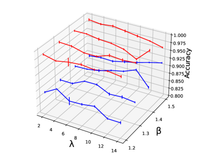
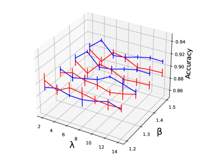
(a) The hyperparameter sensitivity in the Fashion-MNIST detection task. (Blue) The inlier detection accuracy. (Red) The outlier detection arruracy. Error bars represent the mean and standard deviation.

(b) The hyperparameter sensitivity in the credit card fraud detection task. (Blue) The inlier detection accuracy. (Red) The outlier detection arruracy. Error bars represent the mean and standard deviation.

Figure 4: The hyperparameter ($\beta$ and $\lambda$) sensitivity in the Fashion-MNIST dataset and in the credit card fraud detection dataset.

5 Conclusion

In this work, we proposed to robustly approximate OT by regularizing the ordinary OT with the $\beta$-potential term. By leveraging the domain of the Fenchel conjugate of the $\beta$-potential, our algorithm does not move any probability mass to outliers. We demonstrated that our proposed method can be used in estimating a probability distribution robustly even in the presence of outliers and successfully detecting outliers from a contaminated dataset.

SN was supported by JST SPRING, Grant Number JPMJSP2108. MS was supported by JST CREST Grant Number JPMJCR18A2.

Appendix A Details of the Bregman projection

Here, we demonstrate the details of our algorithm inspired by the Non-negative alternate scaling algorithm (NASA) introduced by Dessein et al. (2018), which is an algorithm to obtain the solution for CROT. Although our outlier-robust CROT does not satisfy the assumptions required for CORT, we show our algorithm is constructed similarly to the NASA algorithm.

First, we introduce basics of convex analysis as preliminaries. Next, we explain the alternate scaling algorithm, which is the basis of the NASA algorithm, and the required assumptions for it. Finally, we show the NASA algorithm for the separable Bregman divergence, and how we borrowed their idea to construct our algorithm.

A.1 Convex analysis

Let $\mathcal{E}$ be a Euclidean space with inner product $\langle\cdot,\cdot\rangle$ and induced norm $\|\cdot\|$. The boundary, interior, and relative interior of a subset $\mathcal{S}\subseteq\mathcal{E}$ are denoted by bd($\mathcal{S}$), int($\mathcal{S}$), and ri($\mathcal{S}$), respectively. Recall that for a convex set $\mathcal{C}$, we have

$$\mathrm{ri}(\mathcal{C})=\{\boldsymbol{x}\in\mathcal{E}\ |\ \forall\boldsymbol{y}\in\mathcal{C},\ \exists\lambda>1,\ \lambda\boldsymbol{x}+(1-\lambda)\boldsymbol{y}\in\mathcal{C}\}.$$ (40)

In convex analysis, scalar functions are defined over the whole space $\mathcal{E}$ and take values in $\mathbb{R}\cup\{-\infty,\ \infty\}$. The effective domain, or simply domain, of a function $f$ is defined as the set:

$$\operatorname{dom}f=\{\boldsymbol{x}\in\mathcal{E}\ |\ f(\boldsymbol{x})<+\infty\}.$$ (41)

Definition 3 (Closed functions).

A function $f:\mathbb{R}^{n}\rightarrow\mathbb{R}$ is said to be closed if for each $\alpha\in\mathbb{R}$, the sublevel set $\{\boldsymbol{x}\in\operatorname{dom}f\ |\ f(\boldsymbol{x})\leq\alpha\}$ is a closed set.

If $\operatorname{dom}f$ is closed, then $f$ is closed.

Definition 4 (Proper functions).

Suppose a convex function $f:\mathcal{E}\rightarrow\mathbb{R}\cup\{\pm\infty\}$ satisfies $f(\boldsymbol{x})>-\infty$ for every $\boldsymbol{x}\in\operatorname{dom}f$ and there exists some point $\boldsymbol{x}_{0}$ in its domain such that $f(\boldsymbol{x}_{0})<+\infty$. Then $f$ is called a proper function.

A proper convex function is closed if and only if it is lower semi-continuous. A closed function $f$ is continuous relative to any simplex, polytope of a polyhedral subset in $\operatorname{dom}f$. A convex function $f$ is always continuous in the relative interior ri($\operatorname{dom}f$).

Definition 5 (Essential smoothness Bauschke and Borwein (1997)).

Suppose f is a closed convex proper function on $\mathcal{E}$ with $\mathrm{int}(\operatorname{dom}f)\neq\emptyset$. Then f is essentially smooth, if f is differentiable on $\mathrm{int}(\operatorname{dom}f)$ and

$\begin{array}[]{c}\forall n\in\mathbb{N},\ x_{n}\in\mathrm{int}(\operatorname{dom}f),\\ x_{n}\rightarrow x\in\mathrm{bd}(\operatorname{dom}f)\end{array}\Bigr{\}}\Rightarrow\|\nabla f(\boldsymbol{x}_{n})\|\rightarrow\infty.$

Definition 6 (Essential strict convexity Bauschke and Borwein (1997)).

Let $\partial f$ be the subgradient of $f$. Suppose f is closed convex proper on $\mathcal{E}$. Then, f is essentially strictly convex, if f is strictly convex on every convex subset of $\mathrm{dom(\mathit{\partial f)}}$.

We define a set of functions called the Legendre type and Fenchel conjugate functions.

Definition 7 (Legendre type Bauschke and Borwein (1997)).

Suppose f is a closed convex proper function on $\mathcal{E}$. Then, f is said to be of the Legendre type if f is both essentially smooth and essentially strictly convex.

Definition 8 (Fenchel conjugate Dessein et al. (2018)).

The Fenchel conjugate $f^{*}$ of a function $f$ is defined for all $\boldsymbol{y}\in\mathcal{E}$ as follows:

$$f^{*}(\boldsymbol{y})=\sup_{\boldsymbol{x}\in\mathrm{int}(\operatorname{dom}f)}\langle\boldsymbol{x},\boldsymbol{y}\rangle-f(\boldsymbol{x}).$$ (42)

The Fenchel conjugate $f^{*}$ is always a closed convex function and if $f$ is a closed convex function, then $(f^{*})^{*}=f$, and $f$ is of the Legendre type if and only if $f^{*}$ is of the Legendre type. If $f^{*}$ is of the Legendre type, the gradient mapping $\nabla f$ is a homeomorphism between int(dom$f$) and int(dom$f^{*}$), with inverse mapping $(\nabla f)^{-1}=\nabla f^{*}$. This guarantees the existence of dual coordinate systems $\boldsymbol{x}(\boldsymbol{y})=\nabla f^{*}(\boldsymbol{y})$ and $\boldsymbol{y}(\boldsymbol{x})=\nabla f(\boldsymbol{x})$ on int(dom $f$) and int(dom $f^{*}$).

Finally, we say that a function $f$ is a cofinite if it satisfies

$$\lim_{\lambda\rightarrow+\infty}f(\lambda\boldsymbol{x})/\lambda=+\infty,$$ (43)

for all nonzero $\boldsymbol{x}\in\mathcal{E}$. Intuitively, it means that $f$ grows super-linearly in every direction. In particular, a closed convex proper function is cofinite if and only if $\operatorname{dom}f^{*}=\mathcal{E}$.

A.2 Alternate scaling algorithm

Here, we show the details of obtaining the Bregman projection onto a convex set. Let $\phi$ be a function of the Legendre type with Fenchel conjugate $\phi^{*}=\psi$. In general, computing Bregman projections onto an arbitrary closed convex set $\mathcal{C}\subseteq\mathcal{E}$ such that $\mathcal{C}\cap\mathrm{int}(\operatorname{dom}\phi)\neq\emptyset$ is nontrivial Dessein et al. (2018). Sometimes, it is possible to decompose $\mathcal{C}$ into an intersection of finitely many closed convex sets:

$$\mathcal{C}=\bigcap_{l=1}^{s}\mathcal{C}_{l},$$ (44)

where the individual Bregman projections onto the respective sets $\mathcal{C}_{1},\ldots,\mathcal{C}_{s}$ are easier to compute. It is then possible to obtain the Bregman projections onto $\mathcal{C}$ by alternate projections onto $\mathcal{C}_{1},\ldots,\mathcal{C}_{s}$ according to Dykstra’s algorithm (Boyle and Dykstra, 1986).

In more detail, let $\sigma:\mathbb{N}\rightarrow\{1,\ldots,s\}$ be a control mapping that determines the sequence of subsets onto which we project. For a given point $\boldsymbol{x}_{0}\in\mathrm{int(dom}\phi)$, the Bregman projection $T_{\mathcal{C}}(\boldsymbol{x}_{0})$ of $\boldsymbol{x}_{0}$ onto $\mathcal{C}$ can be approximated with Dykstra’s algorithm by iterating the following updates:

$$\boldsymbol{x}_{k+1}\leftarrow T_{\mathcal{C}_{\sigma(k)}}(\nabla\psi(\nabla\phi(\boldsymbol{x}_{k}+\boldsymbol{y}^{\sigma(k)})),$$ (45)

where the correction term $\boldsymbol{y}^{1},\ldots,\boldsymbol{y}^{s}$ for the respective subsets are initialized with the null element of $\mathcal{E}$, and are updated after projection as follows:

$$\boldsymbol{y}^{\sigma(k)}\leftarrow\boldsymbol{y}^{\sigma(k)}+\nabla\phi(\boldsymbol{x}_{k})-\nabla\phi(\boldsymbol{x}_{k+1}).$$ (46)

Under some technical assumptions, the sequence of updates $(\boldsymbol{x}_{k})_{k\in\mathbb{N}}$ converges in terms of some norm to $P_{\mathcal{C}}(\boldsymbol{x_{0}})$ with a linear rate. Several sets of such conditions have been studied (Dhillon and Tropp, 2007; Bauschke and Lewis, 1993, 2000). Here, we use the following conditions proposed by Dhillon and Tropp [2007] for the CROT framework:

• The function $\phi$ is cofinite

• The constraint qualification $\mathrm{ri}(\mathcal{C}_{1})\cap\cdots\cap\mathrm{ri}(\mathcal{C}_{s})\cap\mathrm{int(dom}\phi)\neq\emptyset$ holds

• The control mapping $\sigma$ is essentially cyclic, that is , there exists a number $t\in\mathbb{N}$ such that $\sigma$ takes each output value at least once during any $t$ consecutive input values

Once these conditions are imposed, the convergence of Dykstra’s algorithm is guaranteed.

A.3 Technical assumptions for CROT to hold

Some mild technical assumptions are required on the convex regularizer $\phi$ and its Fenchel conjugate $\psi=\phi*$ for the CROT framework to hold. The assumptions are as follows:

1. $\phi$ is of Legendre type.

2. $(0,1)^{d\times d}\subseteq\operatorname{dom}\phi$

3. $\operatorname{dom}\psi=\mathbb{R}^{d\times d}$

Some assumptions relate to required conditions for the definition of Bregman projections and convergence of the algorithms, while others are more specific to CROT problems.

The first assumption (1) is required for the definition of the Bregman projection. In addition, it guarantees the existence of dual coordinate systems on int($\operatorname{dom}\phi$) and int($\operatorname{dom}\psi$) via the homeomorphism $\nabla\phi=\nabla\psi^{-1}$.

The second assumption (2) ensures the constraint qualification $\mathcal{G}(\frac{\boldsymbol{1}_{m}}{m},\frac{\boldsymbol{1}_{n}}{n})\cap\mathrm{int}(\operatorname{dom}\phi)$ for the Bregman projection onto the transport polytope.

The third assumption (3) equivalently requires $\phi$ to be cofinite for convergence.

A.4 NASA algorithm

In this subsection, we show the NASA algorithm based on Dykstra’s algorithm constructed by projections on $\mathcal{C}_{0}$,$\mathcal{C}_{1}$, and $\mathcal{C}_{2}$.

Algorithm  NASA algorithm

  $\tilde{\boldsymbol{\theta}}\leftarrow-\boldsymbol{\gamma}/\lambda$

  $\boldsymbol{\theta^{*}}\leftarrow\max\{\nabla\phi(\boldsymbol{0}_{m\times n}),\tilde{\boldsymbol{\theta}}\}$

  repeat

     $\boldsymbol{\tau}\leftarrow\boldsymbol{0}_{m}$

     repeat

        $\boldsymbol{\tau}\leftarrow\boldsymbol{\tau}+\frac{\nabla\psi(\boldsymbol{\theta}^{*}-\boldsymbol{\tau}\boldsymbol{1}_{n}^{\top})\boldsymbol{1}_{n}-\frac{\boldsymbol{1}_{m}}{m}}{\nabla^{2}\psi(\boldsymbol{\theta}^{*}-\boldsymbol{\tau}\boldsymbol{1}_{n}^{\top})\boldsymbol{1}_{n}}$

     until convergence

     $\boldsymbol{\tilde{\theta}}\leftarrow\boldsymbol{\tilde{\theta}}-\boldsymbol{\tau}\boldsymbol{1}_{n}^{\top}$

     $\boldsymbol{\theta^{*}}\leftarrow\max\{\nabla\phi(\boldsymbol{0}_{m\times n}),\boldsymbol{\tilde{\theta}\}}$

     $\boldsymbol{\sigma}\leftarrow\boldsymbol{0}_{n}^{\top}$

     repeat

        $\boldsymbol{\sigma}\leftarrow\boldsymbol{\sigma}+\frac{\boldsymbol{1}_{m}^{\top}\nabla\psi(\boldsymbol{\theta}^{*}-\boldsymbol{1}_{m}\boldsymbol{\sigma})-(\frac{\boldsymbol{1}_{n}}{n})^{\top}}{\boldsymbol{1}_{m}^{\top}\nabla^{2}\psi(\boldsymbol{\theta}^{*}-\boldsymbol{1}_{m}\boldsymbol{\sigma})}$

     until convergence

     $\boldsymbol{\tilde{\theta}}\leftarrow\boldsymbol{\tilde{\theta}}-\boldsymbol{1}_{m}\boldsymbol{\sigma}$

     $\boldsymbol{\theta^{*}}\leftarrow\max\{\nabla\phi(\boldsymbol{0}_{m\times n}),\boldsymbol{\tilde{\theta}}\}$

  until convergence

  $\boldsymbol{\pi^{*}\leftarrow\nabla\psi(\theta^{*})}$

A.4.1 Projcetion onto $\mathcal{C}_{0}$

Let us consider the projection of given matrix $\overline{\boldsymbol{\pi}}$ onto $\mathcal{C}_{0}$. We denote this projection $P_{\mathcal{C}_{0}}(\boldsymbol{\overline{\pi}})$ by $\boldsymbol{\pi}_{0}^{*}$. Then, the Karush-Kuhn-Tucker conditions (Kuhn and Tucker, 1951; Karush, 1939) for $\boldsymbol{\pi}_{0}^{*}$ are as follows:

$$\boldsymbol{\pi}_{0}^{*} \geq \mathbf{0},$$ (47)

$$\nabla\phi(\boldsymbol{\pi}_{0}^{*})-\nabla\phi(\overline{\boldsymbol{\pi}}) \geq \mathbf{0},$$ (48)

$$(\nabla\phi(\boldsymbol{\pi}_{0}^{*})-\nabla\phi(\overline{\boldsymbol{\pi}}))\odot\boldsymbol{\pi}_{0}^{*} = \mathbf{0},\$$ (49)

where (47) is the primal feasibility, (48) is the dual feasibility, and (49) is the complementary slackness.

Since we are thinking of the separable Bregman divergence, the projection onto $\mathcal{C}_{0}$ can be performed with a closed-form expression on primal parameters:

$$\pi^{*}_{0,ij}=\max\{0,\overline{\pi}_{ij}\},$$ (50)

where, $\pi^{*}_{0,ij}$ is the $(i,j)$-element of matrix $\boldsymbol{\pi}_{0}^{*}$. Since $\phi^{\prime}$ is increasing, this is equivalent on the dual parameters of $\boldsymbol{\pi}_{0}^{*}$, $\boldsymbol{\theta}_{0}^{*}$, to

$$\theta_{0,ij}^{*}=\max\{\phi^{\prime}(0),\overline{\theta}_{ij}\}.$$ (51)

Here, the dual coordinate of the input matrix $\overline{\boldsymbol{\pi}}$ is denoted by $\overline{\boldsymbol{\theta}}$.

A.4.2 Projection onto $\mathcal{C}_{1}$ and $\mathcal{C}_{1}$

Next, we consider the Bregman projections of a given matrix $\overline{\boldsymbol{\pi}}\in\mathrm{int(dom}\phi)$ onto $\mathcal{C}_{1}$ and $\mathcal{C}_{2}$. For the projection onto $\mathcal{C}_{1}$ and $\mathcal{C}_{2}$, we employ the method of Lagrange multipliers. The Lagrangians with Lagrange multipliers $\boldsymbol{\mu}\in\mathbb{R}^{m}$ and $\boldsymbol{\nu}\in\mathbb{R}^{n}$ for the Bregman projections $\boldsymbol{\pi}_{1}^{*}$ and $\boldsymbol{\pi}_{2}^{*}$ of a given matrix $\overline{\boldsymbol{\pi}}\in\mathrm{int(dom}\phi)$ onto $\mathcal{C}_{1}$ and $\mathcal{C}_{2}$ respectively write as follows:

$$\mathcal{L}_{1}(\boldsymbol{\pi},\boldsymbol{\mu}) = \phi(\boldsymbol{\pi})-\langle\boldsymbol{\pi},\nabla\phi(\overline{\boldsymbol{\pi}})\rangle+\mu^{\top}(\boldsymbol{\pi}\mathbf{1}-\frac{\mathbf{1}}{m}),$$ (52)

$$\mathcal{L}_{2}(\boldsymbol{\pi},\boldsymbol{\nu}) = \phi(\boldsymbol{\pi})-\langle\boldsymbol{\pi},\nabla\phi(\overline{\boldsymbol{\pi}})\rangle+\nu^{\top}(\boldsymbol{\pi}^{\top}\mathbf{1}-\frac{\mathbf{1}}{n}).$$ (53)

Their gradients are given on int(dom$\phi$) by

$$\nabla\mathcal{L}_{1}(\boldsymbol{\pi},\boldsymbol{\mu}) = \nabla\phi(\boldsymbol{\pi})-\nabla\phi(\overline{\boldsymbol{\pi}})+\boldsymbol{\mu}\mathbf{1}^{\top},$$ (54)

$$\nabla\mathcal{L}_{2}(\boldsymbol{\pi},\boldsymbol{\nu}) = \nabla\phi(\boldsymbol{\pi})-\nabla\phi(\overline{\boldsymbol{\pi}})+\mathbf{1}\boldsymbol{\nu}^{\top},$$ (55)

and vanish at $\boldsymbol{\pi}_{1}^{*},\boldsymbol{\pi}^{*}_{2}\in\mathrm{int(dom}\phi)$ if and only if

$$\boldsymbol{\pi}_{1}^{*} = \nabla\psi(\nabla\phi(\overline{\boldsymbol{\pi}})-\boldsymbol{\mu}\mathbf{1}^{\top}),$$ (56)

$$\boldsymbol{\pi}_{2}^{*} = \nabla\psi(\nabla\phi(\overline{\boldsymbol{\pi}})-\mathbf{1}\boldsymbol{\nu}^{\top}).$$ (57)

By duality, the Bregman projections onto $\mathcal{C}_{1}$, $\mathcal{C}_{2}$ are thus equivalent to finding the unique vectors $\boldsymbol{\mu}$, $\boldsymbol{\nu}$, such that the rows of $\boldsymbol{\pi}_{1}^{*}$ sum up to $\frac{\mathbf{1}}{m}$, respectively the columns of $\boldsymbol{\pi}_{2}^{*}$ sum up to $\frac{\mathbf{1}}{n}$:

$$\nabla\psi(\nabla\phi(\overline{\boldsymbol{\pi}})-\boldsymbol{\mu}\mathbf{1}^{\top})\mathbf{1} = \frac{\mathbf{1}}{m},$$ (58)

$$\nabla\psi(\nabla\phi(\overline{\boldsymbol{\pi}})-\mathbf{1}\boldsymbol{\nu}^{\top})^{\top}\mathbf{1} = \frac{\mathbf{1}}{n}.$$ (59)

Again, since we are resticting ourselves to the separable Bregman divergence, we can compute the projection step more efficiently. Due to the separability, the projections onto $\mathcal{C}_{1}$ and $\mathcal{C}_{2}$ can be divided into $m$ and $n$ parallel subproblems in the search space of 1-dimension as follows:

$$\sum_{j=1}^{n}\psi^{\prime}(\overline{\theta}_{ij}-\mu_{i}) = \frac{1}{m},$$ (60)

$$\sum_{i=1}^{m}\psi^{\prime}(\overline{\theta}_{ij}-\nu_{j}) = \frac{1}{n}.$$ (61)

Here, we denote the dual coordinate of $\overline{\boldsymbol{\pi}}$ by $\overline{\boldsymbol{\theta}}$.

In order to obtain the Lagrange multipliers $\mu_{i}$ and $\nu_{j}$, we use the Newton-Raphson method. More specifically, we eploit the following functions:

$$f(\mu_{i}) = -\sum_{j=1}^{n}\psi^{\prime}(\overline{\theta}_{ij}-\mu_{i}),$$ (62)

$$g(\nu_{j}) = -\sum_{i=1}^{m}\psi^{\prime}(\overline{\theta}_{ij}-\nu_{j}).$$ (63)

These functions are defined on the open intervals $(\hat{\theta}_{i}-\theta_{\mathrm{limit}},+\infty)$ and $(\check{\theta}_{j}-\theta_{\mathrm{limit}},+\infty)$, where $0<\theta_{\mathrm{limit}}<+\infty$ is such that $\operatorname{dom}\psi=(-\infty,\theta_{\mathrm{limit}})$, and $\hat{\theta}_{i}=\max\{\overline{\theta}_{ij}\}_{1\leq j\leq n}$, $\check{\theta}_{j}=\max\{\overline{\theta}_{ij}\}_{1\leq i\leq m}$. We can now obtain the unique solution to $f(\mu_{i})=-\frac{1}{m}$ and $g(\nu_{j})=-\frac{1}{n}$. Starting with $\mu_{i}=0$ and $\nu_{j}=0$, the Newton-Raphson updates:

$$\mu_{i} \leftarrow \mu_{i}+\frac{\sum_{j=1}^{n}\psi^{\prime}(\overline{\theta}_{ij}-\mu_{i})-\frac{1}{m}}{\sum_{j=1}^{n}\psi^{\prime\prime}(\overline{\theta}_{ij}-\mu_{i})},$$ (64)

$$\nu_{j} \leftarrow \nu_{j}+\frac{\sum_{i=1}^{m}\psi^{\prime}(\overline{\theta}_{ij}-\nu_{i})-\frac{1}{n}}{\sum_{i=1}^{m}\psi^{\prime\prime}(\overline{\theta}_{ij}-\nu_{i})},$$ (65)

converge to the optimal solution with a quadraitic rate. To avoid storing the intermediate Lagrange multipliers, the updates can be directly written in terms of the dual parameters:

$$\theta^{*}_{1,ij} \leftarrow \theta^{*}_{1,ij}-\frac{\sum_{j=1}^{n}\psi^{\prime}(\theta^{*}_{1,ij})-\frac{1}{m}}{\sum_{j=1}^{n}\psi^{\prime\prime}(\theta^{*}_{1,ij})},$$ (66)

$$\theta^{*}_{2,ij} \leftarrow \theta^{*}_{2,ij}-\frac{\sum_{i=1}^{m}\psi^{\prime}(\theta^{*}_{2,ij})-\frac{1}{n}}{\sum_{i=1}^{m}\psi^{\prime\prime}(\theta^{*}_{2,ij})},$$ (67)

after initilalization by $\theta^{*}_{1,ij}\leftarrow\overline{\theta}_{ij}$, $\theta^{*}_{2,ij}\leftarrow\overline{\theta}_{ij}$. Here, $\theta_{1,ij}^{*}$ and $\theta_{2,ij}^{*}$ are the $i$th row and $j$th column of $\boldsymbol{\theta}^{*}_{1}$ and $\boldsymbol{\theta}^{*}_{2}$ respectively. $\boldsymbol{\theta}^{*}_{1}$ and $\boldsymbol{\theta}^{*}_{2}$ are the dual coordinates of $\boldsymbol{\pi}^{*}_{1}$ and $\boldsymbol{\pi}^{*}_{2}$ respectively.

From the above, starting from $\boldsymbol{\xi}$ and writing the successive vectors $\boldsymbol{\mu}^{(k)}$, $\boldsymbol{\nu}^{(k)}$ along iterations, we have:

$$\psi^{\prime}(-\boldsymbol{\gamma}/\lambda) \rightarrow \psi^{\prime}\Bigl{(}\max\{\phi^{\prime}(\mathbf{0}),\ -\boldsymbol{\gamma}/\lambda\}\Bigr{)}$$

$$\rightarrow \psi^{\prime}\Bigl{(}\max\{\phi^{\prime}(\mathbf{0}),\ -\boldsymbol{\gamma}/\lambda\}-\boldsymbol{\mu}^{(1)}\mathbf{1}^{\top}\Bigr{)}$$

$$\rightarrow \psi^{\prime}\Bigl{(}\max\{\phi^{\prime}(\mathbf{0}),\ -\boldsymbol{\gamma}/\lambda-\boldsymbol{\mu}^{(1)}\mathbf{1}^{\top}\ )\}\Bigr{)}$$

$$\rightarrow \psi^{\prime}\Bigl{(}\max\{\phi^{\prime}(\mathbf{0}),-\boldsymbol{\gamma}/\lambda-\boldsymbol{\mu}^{(1)}\mathbf{1}^{\top})\}-\mathbf{1}\boldsymbol{\nu}^{(1)\top}\Bigr{)}$$

$$\rightarrow \psi^{\prime}\Bigl{(}\max\{\phi^{\prime}(\mathbf{0}),-\boldsymbol{\gamma}/\lambda-\boldsymbol{\mu}^{(1)}\mathbf{1}^{\top}-\mathbf{1}\boldsymbol{\nu}^{(1)\top}\}\Bigr{)}$$

$$\rightarrow \psi^{\prime}\Bigl{(}\max\{\phi^{\prime}(\mathbf{0}),-\boldsymbol{\gamma}/\lambda-\boldsymbol{\mu}^{(1)}\mathbf{1}^{\top})-\mathbf{1}\boldsymbol{\nu}^{(1)\top}\}+\boldsymbol{\mu}^{(1)}\mathbf{1}^{\top}-\boldsymbol{\mu}^{(2)}\mathbf{1}^{\top}\Bigr{)}$$

$$\rightarrow \psi^{\prime}\Bigl{(}\max\{\phi^{\prime}(\mathbf{0}),-\boldsymbol{\gamma}/\lambda-\boldsymbol{\mu}^{(2)}\mathbf{1}^{\top}-\mathbf{1}\boldsymbol{\nu}^{(1)\top}\}\Bigr{)}$$

$$\rightarrow \psi^{\prime}\Bigl{(}\max\{\phi^{\prime}(\mathbf{0}),-\boldsymbol{\gamma}/\lambda-\boldsymbol{\mu}^{(2)}\mathbf{1}^{\top})-\mathbf{1}\boldsymbol{\nu}^{(1)\top}\}+\mathbf{1}\boldsymbol{\nu}^{(1)\top}-\mathbf{1}\boldsymbol{\nu}^{(2)\top}\Bigr{)}$$

$$\rightarrow \psi^{\prime}\Bigl{(}\max\{\phi^{\prime}(\mathbf{0}),-\boldsymbol{\gamma}/\lambda-\boldsymbol{\mu}^{(2)}\mathbf{1}^{\top}-\mathbf{1}\boldsymbol{\nu}^{(2)\top}\}\Bigr{)}$$

$$\rightarrow \cdots$$

$$\rightarrow \psi^{\prime}\Bigl{(}\max\{\phi^{\prime}(\mathbf{0}),-\boldsymbol{\gamma}/\lambda-\boldsymbol{\mu}^{(k)}\mathbf{1}^{\top}-\mathbf{1}\boldsymbol{\nu}^{(k)\top}\}\Bigr{)}$$

$$\rightarrow \psi^{\prime}\Bigl{(}\max\{\phi^{\prime}(\mathbf{0}),-\boldsymbol{\gamma}/\lambda-\boldsymbol{\mu}^{(k)}\mathbf{1}^{\top}-\mathbf{1}\boldsymbol{\nu}^{(k)\top}\}+\boldsymbol{\mu}^{(k)}\mathbf{1}^{\top}-\boldsymbol{\mu}^{(k+1)}\mathbf{1}^{\top}\Bigr{)}$$

$$\rightarrow \psi^{\prime}\Bigl{(}\max\{\phi^{\prime}(\mathbf{0}),-\boldsymbol{\gamma}/\lambda-\boldsymbol{\mu}^{(k+1)}\mathbf{1}^{\top}-\mathbf{1}\boldsymbol{\nu}^{(k)\top}\}\Bigr{)}$$

$$\rightarrow \psi^{\prime}\Bigl{(}\max\{\phi^{\prime}(\mathbf{0}),-\boldsymbol{\gamma}/\lambda-\boldsymbol{\mu}^{(k+1)}\mathbf{1}^{\top}-\mathbf{1}\boldsymbol{\nu}^{(k)\top}\}+\mathbf{1}\boldsymbol{\nu}^{(k)\top}-\mathbf{1}\boldsymbol{\nu}^{(k+1)\top}\Bigr{)}$$

$$\rightarrow \psi^{\prime}\Bigl{(}\max\{\phi^{\prime}(\mathbf{0}),-\boldsymbol{\gamma}/\lambda-\boldsymbol{\mu}^{(k+1)}\mathbf{1}^{\top}-\mathbf{1}\boldsymbol{\nu}^{(k+1)\top}\}\Bigr{)}$$

$$\rightarrow \cdots$$

$$\rightarrow \boldsymbol{\pi}^{*}.$$

An efficent algorithm then exploits the differences $\boldsymbol{\tau}^{(k)}=\boldsymbol{\mu}^{(k)}-\boldsymbol{\mu}^{(k-1)}$ and $\boldsymbol{\sigma}^{(k)}=\boldsymbol{\nu}^{(k)}-\boldsymbol{\nu}^{(k-1)}$ to scale the rows and columns (Algorithm Algorithm ).

A.5 The different point of our algorithm from NASA

Table 5: Domain of Euclidean norm and $\beta$-potential ($\beta>1$).

Regularization term	dom $\phi$	dom $\psi$
$\beta$-potential ( $\beta>1$ )	$\mathbb{R}_{+}$	$(\frac{1}{1-\beta},\infty)$
Euclidean norm	$\mathbb{R}$	$\mathbb{R}$

An example of applying NASA algorithm is when the regulariler is the Euclidean norm $\phi(\pi)=\frac{1}{2}(\pi-1)^{2}$. As it is shown in Table 5, we can easily confirm the Euclidean norm satisfies the three assumptions introduced in A.3. However, for the outlier-robust CROT, we use $\beta$-potential ($\beta>1$) as the regularizer, which violates the third assumption, $\operatorname{dom}\psi=\mathbb{R}$ (Table 5). Therefore, we cannot naively apply the NASA algorithm for the outlier-robust CROT. For instance, lines 2, 7, and 11 in our algorithm are not mathematically correct as projections onto $\mathcal{C}_{0}$. Similarly, lines 4–6 and 8–10 are not mathematically correct for projections onto $\mathcal{C}_{1}$ and $\mathcal{C}_{2}$, respectively.

In spite of these mathematical issues, we still see lines 2, 7, and 11 in our algorithm as projections onto $\mathcal{C}_{0}$. In addition, since we cannot update the Newton-Raphson more than twice for projections onto $\mathcal{C}_{1}$ and $\mathcal{C}_{2}$ because $\boldsymbol{\theta}^{*}\in\operatorname{dom}\nabla\psi(=\operatorname{dom}\nabla\psi)$ is no longer guaranteed, we overcome this issue by only updating it once.

Appendix B The proof of Proposition 1

Proposition 2.

For a given $z\ (>\frac{\lambda}{\beta-1})$, let $J\subseteq\{1,\ldots,n\}$ be a subset of indices which satisfies the condition shown in Definition 2. Suppose we obtained a transport matrix $\boldsymbol{\pi}^{\mathrm{output}}$ by running the alogrithm $T$ times satisfying the following condition:

$$T<\frac{\frac{z}{\lambda}(\beta-1)-1}{(\frac{1}{m})^{\beta-1}+(\frac{1}{n})^{\beta-1}}.$$ (68)

Then, $\boldsymbol{\pi}^{\mathrm{output}}$ transports no mass to J.

Proof.

Before the algorithm starts,

$$-\frac{z}{\lambda}<\frac{1}{1-\beta}$$ (69)

holds. Since every element in $\boldsymbol{\theta}^{*}$ is greater than or equal to $\phi^{\prime}(0)=\frac{1}{1-\beta}$, the following inequality holds for every $i$ in the algorithm:

$$\tau_{i} \geq \frac{1}{1-\beta}-\phi^{\prime}\Bigl{(}\frac{1}{m}\Bigr{)}$$

$$= \frac{1}{1-\beta}-\left(\frac{1}{\beta-1}\left(\left(\frac{1}{m}\right)^{\beta-1}-1\right)\right)$$

$$= -\frac{1}{\beta-1}\left(\frac{1}{m}\right)^{\beta-1}.$$ (71)

Therefore,

$$-\tau_{i} \leq \frac{1}{\beta-1}\left(\frac{1}{m}\right)^{\beta-1}.$$ (72)

Similarly, for every $j$, the following inequality holds:

$$-\sigma_{j}\leq\frac{1}{\beta-1}\left(\frac{1}{n}\right)^{\beta-1}.$$ (73)

Therefore, if the algorithm finished running $T$ times and the following inequality holds,

$$-\frac{z}{\lambda}+T\times\frac{1}{\beta-1}\left(\frac{1}{m}\right)^{\beta-1}+T\times\frac{1}{\beta-1}\left(\frac{1}{n}\right)^{\beta-1}<\frac{1}{1-\beta},$$ (74)

then,

$$\forall i,\tilde{\theta}_{ij}<\frac{1}{1-\beta}\ \ \mathrm{if}\ \ j\in\textit{J}$$ (75)

holds. Therefore,

$$\forall i,\boldsymbol{\pi}^{\mathrm{output}}_{ij}=0\ \ \mathrm{if}\ \ j\in\textit{J}.$$ (77)

∎

References

- Akram and ul Ann (2015) Sabahat Akram and Qurrat ul Ann. Newton Raphson method. 2015.
- Balaji et al. (2020) Yogesh Balaji, Rama Chellappa, and Soheil Feizi. Robust optimal transport with applications in generative modeling and domain adaptation. In NeurIPS, pages 12934–12944, 2020.
- Basu et al. (1998) Ayanendranath Basu, Ian R. Harris, Nils L. Hjort, and M. C. Jones. Robust and efficient estimation by minimising a density power divergence. Biometrika, 85(3):549–559, 1998.
- Bauschke and Lewis (1993) H. H. Bauschke and A. S. Lewis. Dual coordinate ascent methods for non-strictly convex minimization. Mathematical Programming, 59(1-3):231–247, 1993.
- Bauschke and Lewis (2000) H. H. Bauschke and A. S. Lewis. Dykstra’s algorithm with Bregman projections: A convergence proof. Optimization, 48(4):409–427, 2000.
- Bauschke and Borwein (1997) H.H. Bauschke and J.M. Borwein. Legendre functions and the method of random Bregman projections. Journal of Convex Analysis, 1997.
- Boyle and Dykstra (1986) James P. Boyle and Richard L. Dykstra. A method for finding projections onto the intersection of convex sets in Hilbert spaces. In Advances in Order Restricted Statistical Inference, pages 28–47, New York, NY, 1986. Springer New York.
- Breunig et al. (2000) Markus M. Breunig, Hans-Peter Kriegel, Raymond T. Ng, and Jörg Sander. LOF: Identifying density-based local outliers. SIGMOD Record, 29(2):93–104, 2000.
- Chizat (2017) Lenaic Chizat. Unbalanced Optimal Transport : Models, Numerical Methods, Applications. Theses, Université Paris sciences et Lettres, 2017.
- Clanuwat et al. (2018) Tarin Clanuwat, Mikel Bober-Irizar, Asanobu Kitamoto, Alex Lamb, Kazuaki Yamamoto, and David Ha. Deep learning for classical Japanese literature. CoRR, abs/1812.01718, 2018. URL http://arxiv.org/abs/1812.01718.
- Cohen et al. (2017) Gregory Cohen, Saeed Afshar, Jonathan Tapson, and André van Schaik. EMNIST: an extension of mnist to handwritten letters, 2017. URL https://arxiv.org/abs/1702.05373.
- Cuturi (2013) Marco Cuturi. Sinkhorn distances: Lightspeed computation of optimal transport. In NeurIPS, NIPS’13, page 2292–2300, 2013.
- Deng (2012) Li Deng. The mnist database of handwritten digit images for machine learning research. IEEE Signal Processing Magazine, 29(6):141–142, 2012.
- Dessein et al. (2018) Arnaud Dessein, Nicolas Papadakis, and Jean-Luc Rouas. Regularized optimal transport and the ROT mover’s distance. JMLR, 19(1):590–642, 2018.
- Dhillon and Tropp (2007) I.S. Dhillon and J.A. Tropp. Matrix nearness problems with Bregman divergences. SIAM Journal on Matrix Analysis and Applications, 29(4):1120–1146, 2007.
- Diamond and Boyd (2016) Steven Diamond and Stephen Boyd. CVXPY: A python-embedded modeling language for convex optimization. J. Mach. Learn. Res., 17(1):2909–2913, jan 2016. ISSN 1532-4435.
- Futami et al. (2018) Futoshi Futami, Issei Sato, and Masashi Sugiyama. Variational inference based on robust divergences. In AISTATS, volume 84, pages 813–822. PMLR, 2018.
- Goodfellow et al. (2014) Ian J. Goodfellow, Jean Pouget-Abadie, Mehdi Mirza, Bing Xu, David Warde-Farley, Sherjil Ozair, Aaron Courville, and Yoshua Bengio. Generative adversarial nets. In NeurIPS, page 2672–2680, Cambridge, MA, USA, 2014.
- Kanamori et al. (2009) Takafumi Kanamori, Shohei Hido, and Masashi Sugiyama. A least-squares approach to direct importance estimation. JMLR, 10:1391–1445, 2009.
- Karush (1939) William Karush. Minima of functions of several variables with inequalities as side conditions. Master’s thesis, Department of Mathematics, University of Chicago, Chicago, IL, USA, 1939.
- Knopp and Sinkhorn (1967) Paul Knopp and Richard Sinkhorn. Concerning nonnegative matrices and doubly stochastic matrices. Pacific Journal of Mathematics, 21(2):343 – 348, 1967.
- Kos et al. (2018) Jernej Kos, Ian Fischer, and Dawn Xiaodong Song. Adversarial examples for generative models. 2018 IEEE Security and Privacy Workshops (SPW), pages 36–42, 2018.
- Kuhn and Tucker (1951) H. W. Kuhn and A. W. Tucker. Nonlinear programming. In Proceedings of the Second Berkeley Symposium on Mathematical Statistics and Probability, 1950, pages 481–492, Berkeley and Los Angeles, 1951. University of California Press.
- Kullback and Leibler (1951) S. Kullback and R. A. Leibler. On information and sufficiency. The Annals of Mathematical Statistics, 22(1):79 – 86, 1951.
- Liu et al. (2008) Fei Tony Liu, Kai Ming Ting, and Zhi-Hua Zhou. Isolation forest. 2008 Eighth IEEE International Conference on Data Mining, pages 413–422, 2008.
- Mukherjee et al. (2021) Debarghya Mukherjee, Aritra Guha, Justin M Solomon, Yuekai Sun, and Mikhail Yurochkin. Outlier-robust optimal transport. In ICML, pages 7850–7860, 2021.
- Pedregosa et al. (2011) Fabian Pedregosa, Gaël Varoquaux, Alexandre Gramfort, Vincent Michel, Bertrand Thirion, Olivier Grisel, Mathieu Blondel, Peter Prettenhofer, Ron Weiss, Vincent Dubourg, Jake Vanderplas, Alexandre Passos, David Cournapeau, Matthieu Brucher, Matthieu Perrot, and Édouard Duchesnay. Scikit-learn: Machine learning in Python. JMLR, 12:2825–2830, 2011.
- Peyré and Cuturi (2019) Gabriel Peyré and Marco Cuturi. Computational optimal transport. Foundations and Trends in Machine Learning, 11 (5-6):355–602, 2019.
- Rabin et al. (2012) Julien Rabin, Gabriel Peyré, Julie Delon, and Marc Bernot. Wasserstein barycenter and its application to texture mixing. In Scale Space and Variational Methods in Computer Vision, pages 435–446, 2012.
- Rousseeuw and van Driessen (1999) Peter J. Rousseeuw and Katrien van Driessen. A fast algorithm for the minimum covariance determinant estimator. Technometrics, 41(3):212–223, 1999.
- Schölkopf et al. (1999) Bernhard Schölkopf, Robert Williamson, Alex Smola, John Shawe-Taylor, and John Platt. Support vector method for novelty detection. In NeurIPS, 1999.
- Solomon et al. (2015) Justin Solomon, Fernando de Goes, Gabriel Peyré, Marco Cuturi, Adrian Butscher, Andy Nguyen, Tao Du, and Leonidas Guibas. Convolutional Wasserstein distances: Efficient optimal transportation on geometric domains. ACM Transactions on Graphics, 34(4), 2015.
- Staerman et al. (2021) Guillaume Staerman, Pierre Laforgue, Pavlo Mozharovskyi, and Florence d’Alché Buc. When OT meets MoM: Robust estimation of wasserstein distance. In AISTATS, volume 130, pages 136–144, 2021.
- Villani (2008) Cédric Villani. Optimal transport – Old and new, volume 338. Springer Berlin, Heidelberg, 2008.
- Xiao et al. (2017) Han Xiao, Kashif Rasul, and Roland Vollgraf. Fashion-MNIST: a novel image dataset for benchmarking machine learning algorithms. CoRR, 2017.