E-AFE: Approximate Hashing for Automated Feature Engineering

Accelerating Automated Feature Engineering via Sample Hashing

Toward Efficient Automated Feature Engineering

Abstract

Automated Feature Engineering (AFE) refers to automatically generate and select optimal feature sets for downstream tasks, which has achieved great success in real-world applications. Current AFE methods mainly focus on improving the effectiveness of the produced features, but ignoring the low-efficiency issue for large-scale deployment. Therefore, in this work, we propose a generic framework to improve the efficiency of AFE. Specifically, we construct the AFE pipeline based on reinforcement learning setting, where each feature is assigned an agent to perform feature transformation and selection, and the evaluation score of the produced features in downstream tasks serve as the reward to update the policy. We improve the efficiency of AFE in two perspectives. On the one hand, we develop a Feature Pre-Evaluation (FPE) Model to reduce the sample size and feature size that are two main factors on undermining the efficiency of feature evaluation. On the other hand, we devise a two-stage policy training strategy by running FPE on the pre-evaluation task as the initialization of the policy to avoid training policy from scratch. We conduct comprehensive experiments on 36 datasets in terms of both classification and regression tasks. The results show $2.9\%$ higher performance in average and 2x higher computational efficiency comparing to state-of-the-art AFE methods.

I Introduction

Feature engineering refers to the process of feature generation and selection to convert raw data into effective features for machine learning tasks. Due to the lack of domain knowledge, traditional manual feature engineering is labor-intensive and time-consuming [1]. To overcome the limitation, Automated Feature Engineering (AFE) is proposed to automatically generate and select optimal feature sets [2, 3]. On the one hand, AFE can significantly reduce human efforts and benefit the deployment in large-scale big data systems; on the other hand, AFE can also discover new knowledge from the data that is hardly achieved by traditional manual data engineering.

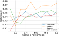
(1) Sample Percentage vs. Performance.

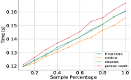
(2) Sample Percentage vs. Computation Time.

Figure 1: Sample size vs. performance and computation Time.

Current studies in AFE focus on leveraging the Reinforcement Learning paradigm to explore possible feature candidates and exploit generated features to downstream machine learning tasks for selecting optimal feature sets. For example, Nargesian et al. proposed Learning Feature Engineering (LFE) with focusing on extracts useful transformations from past feature engineering experiences [4]; Khurana et al. developed a new transformation graph with Directed Acyclic Graph (DAG) to represent relationships between different transformed versions of the data, and Q-learning was used to learn a performance-guided strategy for effective feature transformation from historical instances [5]. In order to resolve the feature space explosion problem on high-order transformations, Chen et al. proposed Neural Feature Search (NFS) that utilized Recurrent Neural Network (RNN)-based controller to transform each raw feature through a series of transformation functions, and policy gradient was used to train this controller [6].

Dataset	Instances$\backslash$Features	New Features	Generation Time	Eval. New Features Time	Total Time
PimaIndian	768$\backslash$8	1195	354ms	205s	225s
credit-a	690$\backslash$6	890	192ms	139s	155s
diabetes	768$\backslash$8	1174	334ms	203s	223s
german credit	1001$\backslash$24	3730	1291ms	654s	732s

TABLE I: One epoch of NFS time consuming on four datasets.

While promising feature sets produced, these state-of-the-art AFE methods suffer from low-efficiency issue, especially in terms of time consumption for complex machine learning tasks. Taking NFS as an example. We investigate the time consumption of NFS on four datasets with different sizes, and present the empirical results in Table I. The results show that for each dataset, only about 0.1% of the time is spent on feature generation, but about 90% of the time is consumed on evaluating new features. The observation indicates that the efficiency of AFE is largely impeded by the feature evaluation step. Moreover, with the sample size increasing, the feature evaluation would take much more time, which even exacerbates the low-efficiency issue. Unfortunately, few efforts are put on improving the efficiency of AFE methods.

Therefore, in this work, we aim to study how to accelerate AFE. As the feature evaluation step takes the most of time, we propose to improve the efficiency of AFE by optimizing the feature evaluation process. Specifically, we optimize the feature evaluation process from two perspectives: (1) reducing the sample size for evaluation; (2) reducing the size of candidate features for evaluation. Next, we introduce the two perspectives as follows:

(1) Reducing the sample size for evaluation. In traditional pipeline of AFE, the feature evaluation is conducted over the whole dataset. However, not all samples are necessary for determining the quality of the generated features. We empirically investigate the contribution of the sample size on the feature performance. Specifically, we randomly sample different percentage of four datasets, and calculate the performance of the selected features and the corresponding running time. We conduct the operation for ten times, and present the average results in Figure 1. The results show that ignoring when the sample size achieves a certain scale, the performance of the selected features remains relatively stable. With more samples getting involved in, it barely enhances the quality of the selected features, but raises unacceptable surge in time consumption. The observation suggests that reducing the sample size is a promising direction for accelerating the feature evaluation process without sacrificing the feature quality.

(2) reducing the size of candidate features for evaluation. In addition to sample size, the size of candidate features is another important factor to affect the running time of evaluation. Intuitively, more features lead to larger candidate space for evaluation in feature selection, resulting in larger running time. Moreover, traditional AFE methods directly evaluate the features on the downstream tasks. However, the downstream tasks are usually complex and time-consuming, which even significantly retards the feature evaluation process. Therefore, reducing the size of candidate features prior to the formal evaluation (downstream tasks) is a potential solution.

Nevertheless, it is challenging to achieve the goal. The reasons are as follows: First, since AFE aims to provide a generic feature-refinement pipeline for different datasets with various sizes, the reducing process demands to work for arbitrary sample sizes. Second, different datasets have features with diverse semantic meanings, thus, how to determine a feature as a candidate for evaluation across datasets in a unified manner is non-trivial. Third, it is even more challenging to combine reducing the size of samples and candidate features without violating each requirement. Therefore, to tackle the above challenges, we propose to develop a simple and fast yet reasonable auxiliary evaluation task to pre-evaluate the validness of features to filter the candidate features prior to the formal evaluation. The proposed auxiliary evaluation task, namely Feature-Validness Task, is a binary classification task that justifies whether one feature is selected as a candidate for the formal evaluation. The Feature-Validness Task takes features as input, where one feature is denoted by respective values in samples. We pre-train a binary classification model, namely Feature Pre-Evaluation (FPE) Model, for the Feature-Validness Task using a group of public datasets as prior knowledge, and apply the well-trained model for pre-evaluation of the candidate features. In this case, all the features are required to be represented as a fixed size of samples. To achieve the goal, we further propose a Hashing-based method to project arbitrary sample sizes into a fixed number, which naturally fulfill the requirement for reducing sample sizes.

Along this line, we propose an efficient AFE framework with accelerating AFE via reducing the size of samples and candidate features simultaneously. Specifically, we formulate AFE as an off-policy reinforcement learning problem following the convention of AFE. Different from existing AFE methods, generated features from agents would be first pre-evaluated by the pre-trained FPE model to reduce the feature size with compressing samples to improve the efficiency. Then, to further reduce the costs on exploring promising feature transformation actions, we develop a two-stage training strategy: (1) quick initialization with FPE model, and (2) formal training. In stage 1, we only use FPE model as the evaluation to quickly discover promising feature transformation actions. During stage 1, the policy is initialized by borrowing knowledge from the pre-trained FPE model, and one replay buffer is constructed to record potentially good actions. After several epochs of training in stage 1, we formally convert the evaluation to the downstream tasks in stage 2. Trough this way, the proposed framework can improve the training efficiency by avoiding learning the policy from scratch. Our contributions can be listed as follows:

• To the best of our knowledge, we are the first to study how to improve the efficiency of AFE.

• Through empirical studies, we identify the core reason of the low-efficiency issue of AFE as the inefficient feature evaluation process.

• We propose an efficient AFE framework by reducing the size of samples and candidate features simultaneously through a faster auxiliary feature evaluation task with sample hashing.

• We develop a two-stage training strategy to improve the efficiency of policy learning.

• We conduct comprehensive experiments on 36 datasets in terms of both classification and regression tasks. The results show $2.9\%$ higher performance in average and 2x higher computational efficiency comparing to state-of-the-art methods.

II Problem Formulation

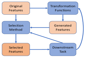
(1) General Process of Automated Feature Engineering

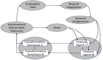
(2) Automated Feature Engineering with RL

Figure 2: From traditional AFE to RL-based AFE.

In this section, we introduce the formulation of AFE. For tabular datasets, the general pipeline of AFE can be abstracted into two steps: feature generation and selection. As shown in Figure 2(1), the original features are first transformed into generated features through a series of combinatorial transformation functions. Then the selection method selects effective features from the generated features based on the evaluation results in downstream tasks. Then, the evaluation results will be further used as the feedback to improve the selection method and transformation functions to continue generating and selecting features until the selected features satisfy the evaluation requirement for the downstream tasks. Formally, given a dataset $\mathcal{D}\langle\mathbf{F},\mathbf{y}\rangle$ with $N$ original features $\mathbf{F}=\{f^{[1]},f^{[2]},...,f^{[N]}\}$ with label $\mathbf{y}$, we use $A_{\mathcal{T}}(\mathbf{F},\mathbf{y})$ to represent the evaluation score of the downstream task $\mathcal{T}$ on dataset $\mathcal{D}$. The original feature set $\mathbf{F}$ is transformed into $\mathbf{\check{F}}$ through a set of transformation functions (e.g., addition, multiplication, logarithm, etc). The AFE is to find the optimal transformed feature set $\mathbf{F}^{*}$ where $A_{\mathcal{T}}(\mathbf{F}^{*},\mathbf{y})$ is maximized, such that $\mathbf{F}^{*}=\underset{\mathbf{\check{F}}}{\mathrm{argmax}}{A_{\mathcal{T}}(\mathbf{\check{F}},\mathbf{y})}$.

In this work, we formulate AFE in a reinforcement learning setting, as shown in Figure 2(2). We outline the definitions for the key elements as follows:

• Environment. In our design, the environment is the feature subspace of generated feature space. Whenever a feature agent issues an action to generate a new feature, the state of the feature subspace (environment) changes.

• Agents. Suppose there are $N$ original features in the dataset, we define $N$ agents to generate features. Specifically, each agent will generate new features based on the given original feature. In other words, considering one original feature and the respective newly generated features as a subgroup of the state space, there are $N$ feature subgroups. Each agent will be responsible for one feature subgroup.

• State Space. We define the state $s$ as the selected features. The dimension (size) of the state space is the size of the selected feature. The selected features include the original features and the newly generated features. Once a newly generated feature is discriminated as a good feature, the feature will be included into the state. Therefore, with more newly generated features added into the state, the state space will keep expanding until the feature engineering process finishes.

• Action. We define the action $a$ as the feature transformation. Each agent will take actions (feature transformation) over the respective feature subgroup. The feature transformation is in the format of $\text{OPERATOR}(\text{feature}_{1},\text{feature}_{2})$, where OPERATOR is a feature transformation operator that takes two features as input and outputs a new feature, and $\text{feature}_{1}$ and $\text{feature}_{2}$ are two features from one feature subgroup. We consider two types of feature transformation operators: (i) unary operator (including logarithm, min-max-normalization, square root, and reciprocal), in this case, $\text{feature}_{1}$ and $\text{feature}_{2}$ are the same feature; (ii) binary operator (including addition, subtraction, multiplication, division, and modulo operation), in this case, $\text{feature}_{1}$ and $\text{feature}_{2}$ are two different features.

• Transition. We illustrate the transition process in Figure 3. For simplicity, we take the transition from $s_{t}$ to $s_{t+1}$ as an example. The agent first sample two features from the respective feature subgroup in $s_{t}$ with replacement. Then, the agent takes actions according to the policy to generate new features. The newly generated features will be discriminated as qualified or unqualified. Once confirmed as qualified, the newly generated feature will be selected and added to the respective feature subgroup to construct new state $s_{t+1}$.

  

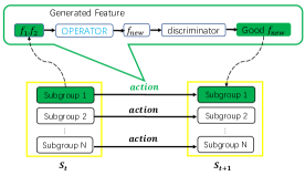
  Figure 3: The transition process.

• Evaluation Task. The evaluation task aims to examine the effectiveness of the generated and selected features. There are two types of evaluation tasks: (1) pre-evaluation task, that is to reduce the feature size through quick binary classification; and (2) downstream task, that is the formal evaluation task to evaluate and select the generated features. Following the convention of AFE [6], we utilize Random Forest as the model for downstream tasks. Details will be introduced in Section III-B.

• Reward. We define the performance gain on the evaluation task as the reward $r$.

Figure 4: An illustration of feature generation using RNN-based agent. An RNN implements an agent of the raw feature. $s_{t}$ is state, $a_{t}$ is action, $h_{t}$ is action probability distribution, $f_{t}$ is generated features, $r_{t}$ is the reward of new features. The initial state is the original feature. The evaluation task returns the reward $r_{t}$ to the $h_{t}$ through backpropagation on the loss function Equ. LABEL:equ:rnn_loss and updates $h_{t}$.

Based on the above definition, we take one agent as example to show how the proposed RL-based AFE generates features. For each feature, we exploit a RNN as the agent to take actions. Specifically, we maintain the hidden state of RNN as the probability distribution to sample an action (feature transformation function) to perform. For the first round generation, we set the action probability distribution as uniform distribution, and the original feature set as the input. For the $t$-th round generation, we take the probability distribution $h_{t-1}$ updated from the $(t-1)$-th round generation, and current state (feature set) $s_{t}$ of RL as the input to RNN. RNN would output the updated probability distribution $h_{t}$. We sample an action $a_{t}$ based on the updated probability distribution $h_{t}$. Then, we generate new features $f_{t}$ by applying the action $a_{t}$ on the feature set $s_{t}$. The updated state (feature set) $s_{t+1}$ is the combination of the input feature set $s_{t}$ and the generated feature set $f_{t}$. Moreover, the generated features $f_{t}$ will be evaluated on the evaluation tasks and obtain the reward $r_{t}$. The action probability distribution $h_{t}$ will be further updated based on the reward $r_{t}$ by Equ. LABEL:equ:rnn_loss. Finally, the updated distribution $h_{t}$ will be taken as the hidden state of RNN to perform the next round feature generation.

The loss function of our RNN is as Equ. LABEL:equ:rnn_loss. Agent loss function is constructed by three parts. $r$ is the reward, $h$ is the action probability distribution, and $\theta$ is the weight of RNN.

$$\begin{split}&\mathcal{L}(\theta,h,r)=\log(\mathrm{argmax}(h))*r+\log(h)*h+||\theta||^{2}\\ \end{split}$$ (1)

TABLE II: Notations for E-AFE

Notations	Meaning
$\mathcal{D}\langle\mathbf{F},\mathbf{y}\rangle$	Dataset $\mathcal{D}$ with feature $\mathbf{F}$ and label $\mathbf{y}$
$\mathcal{T}$	Downstream task (classification or regression)
$A_{\mathcal{T}}(\mathbf{F},\mathbf{y})$	Score of a downstream task $\mathcal{T}$ on $(\mathbf{F},\mathbf{y})$
$\mathbf{\check{F}}$	A set of generated feature
$\mathcal{D}^{i}$	The $i$-th taining set
$\mathcal{D}^{i}_{j}$	The $i$-th residual dataset (drawed $j$-th feature)
$\mathcal{V}$	Validation set
$A^{i}_{0}$	The score of $i$-th original training set
$A^{i}_{j}$	The score of residual dataset $\mathcal{D}^{i}_{j}$
$d$	MinHash signature output dimension
H	Approximate hashing features
L	Labels of negative/positive feature (0 or 1)
$thre$	Threshold of score gain for feature labels (0 or 1)
$Rec,Prec$	Recall, Precision
$\mathcal{C}_{\mathcal{D}}$	The FPE model
$N$	The number of features on a target dataset
$T$	Sample of an episode
$s_{t}$	State at time $t$ for one agent
$a_{t}$	Action at time $t$ of one agent
$r_{t}$	Reward at time $t$ of one agent
$\gamma$	Discount factor in range [0,1]
$h_{t}$	Action probability distribution at time $t$ of one agent

The notations used in this paper are summarized in Table II.

III E-AFE

In this section, we introduce our proposed framework in detail. We start with overall framework of our proposed E-AFE. Then, we present FPE model for reducing sample and feature size. Moreover, we introduce the two-stage training strategy for enhancing the learning efficiency. Finally, we provide a theoretical analysis of the algorithm complexity.

III-A Framework Overview

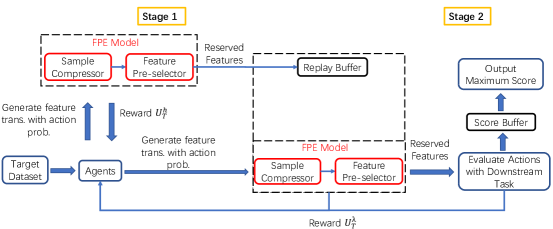
Figure 5: Framework Overview.

Figure 5 shows an overview of the proposed framework. The core elements of  E-AFE  includes two parts: (1) FPE model, which is to reduce the sample size and candidate feature size for improving the evaluation efficiency; (2) two-stage policy-training strategy, which is to boost the learning efficiency by avoiding training from scratch. Specifically, for each original feature, the agent will first generate features following the pipeline as shown in Figure 4. Then, the generated features are fed into the FPE model to reduce sample size with the hashing module, and reduce the candidate feature size with a binary classifier pre-trained by the pre-evaluation task. During the policy training procedure, we will initialize the policy with taking the pre-evaluation task as the evaluation task to train for several epochs. Meanwhile, we construct a replay buffer to record promising actions. Then, we continue to train the policy with real downstream tasks. The proposed framework continue to be trained until the optimal features are achieved.

III-B Feature Pre-Evaluation (FPE) Model

As discussed in Section I, sample size and feature size are two vital factors to compromise the efficiency of AFE. Therefore, we develop FPE model to help reduce the sample and feature size to accelerate AFE. Specifically, FPE model consists of two modules: (1) sample compressor, which is to reduce sample size with hashing operations; and (2) feature pre-selector, which is to reduce candidate feature size for evaluation tasks with pre-trained binary classifier.

Sample Compressor. Figure 1 indicates that not all samples are necessary for feature evaluation. Therefore, a method for reducing the sample size is highly desired. Moreover, different datasets have various sizes. To be generalized across datasets, the compression method also expects to compress arbitrary input sizes into the fix one. Therefore, in this work, we adopt hashing techniques as the sample compressor to reduce sample size. Specifically, we take MinHash as the hashing function family. The basic idea of MinHash is to assign the target dimension hashing values, and select $d$ instances with the minimum hashing values as the compressed results [7].

In our sample compressor case, given a dataset (tabular data) $\mathcal{D}\in\mathbb{R}^{M\times N}$ with $N$ features (column) and $M$ samples (row). We take samples (row) as the target dimension, and input into MinHash. Suppose the expected sample size is $d$, we expect the compressed dataset with selected $d$ samples should also preserve the sample similarities in the original $M$-sample dataset. Then the compression process can be represented as

$$\begin{split}\tilde{\mathcal{D}}&=\text{MinHash}(\mathcal{D},d),\\ ~{}s.t.~{}|\text{sim}&(\mathcal{D}^{1},\mathcal{D}^{2})-\text{sim}(\tilde{\mathcal{D}}^{1},\tilde{\mathcal{D}}^{2})|<\epsilon\\ \end{split}$$ (2)

where $\mathcal{D}\in\mathbb{R}^{M\times N}$ and $\tilde{\mathcal{D}}\in\mathbb{R}^{d\times N}$ denote the orignal dataset and compressed dataset, respectively, and $\epsilon$ denotes a very small constant. $D^{1}$ and $D^{2}$ are the two datasets whose similarity is to be calculated.

Feature Pre-Selector. Since evaluating features directly on downstream tasks is time-consuming, we develop a fast yet effective pre-evaluation task to pre-select candidate features. Specifically, we pre-train a binary classifier on public datasets to distinguish the effective features from the generated feature set. Formally, given $n$ public datasets, and each dataset is $\mathcal{D}^{i}=[k^{i},m^{i}],i\in[1,n]$, which include $m^{i}$ original features and $k^{i}$ instances. The downstream task $\mathcal{T}$ calculates the original performance score as $A_{0}$. Then, we leave out the $j$-th feature from $i$-th original dataset to construct the residual dataset $\mathcal{D}^{i}_{j}$. We continue to calculate the performance score $A_{j}^{i}$ for $\mathcal{D}^{i}_{j}$. We compare the performance score between $A_{0}$ and $A_{j}^{i}$ to determine whether the $j$-th feature is effective. Then, the labeling process of feature effectiveness can be represented as

$$\begin{split}&\mathbf{A}_{0}^{i}=\mathcal{T}(\mathcal{D}^{i}),~{}i\in[1,n]\\ &\mathcal{D}_{j}^{i}\leftarrow\mathcal{D}^{i}-\mathbf{F}_{j}^{i}\\ &\mathbf{A}_{j}^{i}=\mathcal{T}(\mathcal{D}_{j}^{i}),~{}j\in[1,m^{i}],i\in[1,n]\\ &\mathbf{L}_{j}^{i}=\mathrm{sgn}(\mathbf{A}_{0}^{i}-\mathbf{A}_{j}^{i}+thre)\end{split}$$ (3)

where $thre$ is the threshold of score gain; $\mathrm{sgn}(z)=1$ if $z>0$ and $\mathrm{sgn}(z)=0$ (or equivalently -1) otherwise; $\mathbf{L}$ is the label vector. Consequently, the effective feature is labeled as $1$, otherwise $0$. $thre$ is set a small value, such as 0.01. This value is to set the boundary of the binary classification, which is larger than 0, so that better features can be found. If set to 0, many features that are not significantly improved for downstream tasks may be retained. The size of this threshold is also set according to the recall effect. For example, as shown in Figure 6.

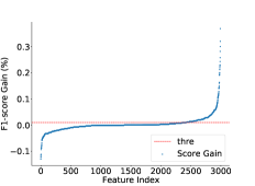
Figure 6: The $thre$ and score gain for classification.

Once the label vector is obtained, we pre-train a binary classifier $\mathcal{C}_{\mathcal{D}}$ paramterized by $\phi$ through taking the sample-compressed features as input. We select effective features (labeled as $1$) as the candidate as the input to evaluation tasks in RL-based AFE. Although the pre-evaluation task is still based on real downstream tasks, once well-trained, the binary classifier can infer the effectiveness of given features quickly.

Model Optimization. We exploit cross-entropy as the loss function and take maximizing recall as the optimization target. The objective is to find the optimal sample compressor with the optimal compression size $d$ complying with best feature-effectiveness classifier. Therefore, we consider the sample compressor as the hyperparameter by fine-tuning the hashing function options and compression size $d$ to train the feature-effectiveness classifier. Formally, the predicted label vector $\tilde{\mathbf{L}}$ can be represented as

$$\begin{split}\mathbf{H}&=\text{MinHash}(\mathcal{D},d)\\ \tilde{\mathbf{L}}&=\mathrm{sgn}(\mathcal{C}_{\mathcal{D}}(\mathbf{H}))\\ \end{split}$$ (4)

Then, according to the ground-truth $\mathbf{L}$ and prediction $\tilde{\mathbf{L}}$, we calculate the precision $Prec$ and recall $Rec$ as

$$\begin{split}Prec&=\text{Precision}(\mathbf{L},\tilde{\mathbf{L}})\\ Rec&=\text{Recall}(\mathbf{L},\tilde{\mathbf{L}})\\ \end{split}$$ (5)

Then, the objective can be represented as

$$\begin{split}&\mathcal{C}_{\mathcal{D}}^{*},\text{MinHash}^{*},d^{*}\leftarrow\underset{\mathcal{C}_{\mathcal{D}},\text{MinHash},d}{\mathrm{argmax}}~{}Rec,\\ &~{}s.t.~{}Prec>0~{}and~{}Rec<1,\\ \end{split}$$ (6)

where $\mathcal{C}_{\mathcal{D}}^{*}$, $\text{MinHash}^{*}$ and $d^{*}$ are optimal classifier, and the corresponding hashing function and compressed sample size, respectively. We perform stochastic gradient descent (SGD) to train and fine-tune the FPE model. Algorithm 1 shows the calculation details of FPE model.

Algorithm 1 Feature Pre-Evaluation (FPE) Model

Input: $n$ public dataset $\mathcal{D}$ for training, every dataset has $k^{i},i\in[1,n]$ samples and $m^{i},i\in[1,n]$ features. $\mathcal{V}$ is the validation set. $\mathcal{T}$ is the downstream task. $\mathbf{d}$ is the vector of MinHash signature output dimension for an approximate feature. $thre$ is the threshold of score gain for feature labels (0 or 1). MinHash is hash function set.
Output: Trained FPE model $\mathcal{C}_{\mathcal{D}}$, MinHash function and MinHash output dimension $d$.

1:  while Select $d\in\textbf{d}$ or MinHash Function do

2:     Let $\mathbf{A}=[],\mathbf{L}=[],Rec=[]$.

3:     /*Training model with cross-entropy*/

4:     for $i=1\rightarrow n$ do

5:        Get $\mathbf{A}_{0}^{i}$ by Equ. (LABEL:equ:acc0_label) on $\mathcal{D}^{i}$.

6:        for $j=1\rightarrow m^{i}$ do

7:           Draw sub dataset $\mathcal{D}_{j}^{i}\leftarrow\mathcal{D}^{i}-\mathbf{F}_{j}^{i}$.

8:           Get $\mathbf{A}_{j}^{i}$ by Equ. (LABEL:equ:acc0_label) on $\mathcal{D}_{j}^{i}$.

9:           if $\mathbf{A}_{0}^{i}-\mathbf{A}_{j}^{i}>thre$ then

10:              $\mathbf{L}_{j}^{i}\leftarrow 1$

11:           else

12:              $\mathbf{L}_{j}^{i}\leftarrow 0$

13:           end if

14:           $\mathbf{H}_{j}^{i}\leftarrow\text{MinHash}(\mathbf{F}_{j}^{i},d)$ as Equ. (4)

15:        end for

16:     end for

17:     /*Validating model for recall*/

18:     $\tilde{\mathbf{L}}=\mathrm{sgn}(\mathbf{\mathcal{C}}_{\mathcal{D}}(\mathbf{H}))$ as Equ. (4)

19:     $Rec=\text{Recall}(\mathbf{L},\tilde{\mathbf{L}})$ as Equ. (5)

20:  end while

21:  /*Train and fine-tune the FPE model*/

22:  $\mathcal{C}_{\mathcal{D}}^{*},\text{MinHash}^{*},d^{*}\leftarrow\underset{\mathcal{C}_{\mathcal{D}},\text{MinHash},d}{\mathrm{argmax}}(Rec)$ as Equ. (LABEL:equ:argmax)

23:  return $\mathcal{C}_{\mathcal{D}}^{*},\text{MinHash}^{*},d^{*}$

Algorithm 2 Two-Stage Policy Training Strategy

Input: Trained FPE model $\mathcal{C}_{\mathcal{D}}$. Features $\mathbf{F}$ of the target dataset. MinHash function. MinHash output dimension $d$.
Output: Maximize score of downstream task

1:  /*Stage 1: Quick Initialization with FPE Model*/

2:  while Choose agent one by one do

3:     Agent sample action with equal rate

4:     Action generates new feature $\check{f}\in\mathbf{\check{F}}$

5:     Evaluate $\check{f}$ by Equ. (LABEL:equ:probability)

6:     if $\check{f}$ is positive feature then

7:        Store this feature to replay buffer

8:     else

9:        Dropout this feature

10:     end if

11:     Get $A^{h}_{t}$ by Equ. (8)

12:     Get return $U^{h}_{t}$ by Equ. (LABEL:equ:return_single) for every agent

13:  end while

14:  Agents initialization complete

15:  /*Stage 2: Formal Training*/

16:  while Get feature from replay buffer do

17:     Sample feature transformation with action prob.

18:     Generate new features by transformation

19:     Save score of the downstream task

20:     Get return $U^{\lambda}_{t}$ by Equ. (LABEL:equ:return_multi).

21:  end while

22:  Trained agents

23:  return Maximize score of downstream task

III-C Two-Stage Training Strategy

We integrate the well-trained FPE model into the RL-based AFE framework to construct  E-AFE , as shown in Figure 5. The conventional training process of RL-based AFE methods suffer from exhaustively exploring the action-state space, which wastes a lot of running time to reach the optimum. Therefore, to solve the problem, we propose the two-stage training strategy by borrowing external knowledge from pre-trained FPE model to avoid learning policy from scratch. The two-stage training strategy includes: (1) quick initialization with FPE model, and (2) formal training.

Stage 1: Quick Initialization with FPE Model The benefits of FPE model lie in two aspect. On the one hand, FPE model is trained on various public datasets, which contain rich external knowledge of feature characteristics; On the other hand, the well-trained FPE can directly infer the effectiveness of the generated features, which saves substantial time comparing to the downstream task evaluation. Therefore, at the initialization stage, we omit the downstream task evaluation, but directly take the results from FPE model as the reward to update the policy of  E-AFE . Formally, we compute the reward of each action as follows: for taking action $a_{t}$, the improvement $r_{t}$ is the score $A_{t}$ of state $s_{t}$ minus $A_{t-1}$ of state $s_{t-1}$ , which means the gain of performing $a_{t}$ intuitively. Then, we utilize the $\lambda-return$ $U^{\lambda}_{t}$ that combines all $k-step$ returns $U_{t}$ as the final reward signal for action $a_{t}$. We define $A^{O}$ and $A^{h}$ as the performance score of the original dataset and compressed dataset by FPE model, respectively. $\Delta A_{max}$ and $\Delta A_{min}$ are the maximize and minimize score gain of input space. Then, the accumulated reward can be computed as

$$\begin{split}&p=\mathcal{C}_{\mathcal{D}}(\text{MinHash}(\check{f},d))\\ \end{split}$$ (7)

$$A^{h}_{t}=\left\{\begin{aligned} A^{O}+\frac{0.5-p}{0.5}(\Delta A_{max}-thre),p\in[0,0.5)\\ A^{O}+\frac{0.5-p}{0.5}(thre-\Delta A_{min}),p\in[0.5,1]\\ \end{aligned}\right.$$ (8)

where, $thre$ is the threshold of score gain for feature labels (0 or 1). $\check{f}$ is a new feature from the test set. $p$ is the output probability of the binary classifier.

$$\begin{split}&r^{h}_{t}=A^{h}_{t}-A^{h}_{t-1}\\ &U^{h}_{t}=r^{h}_{t}+\gamma r^{h}_{t+1}+...+\gamma^{k}r^{h}_{t+k}=\sum^{t}_{k=0}\gamma^{(t-k)}r^{h}_{k}\\ \end{split}$$ (9)

Stage 2: Formal Training After several epochs of training in stage 1, we then change the evaluation task to the real downstream task. We take the output of FPE model (pre-selected feature with reduced sample and feature size) as the candidate features to formally train the policy, where the reward is computed as the performance gain on the downstream tasks. To be consistent with the stage 1, we represent the accumulated rewards for stage 2 as:

$$\begin{split}&r_{t}=A_{t}-A_{t-1}\\ &U_{t}=r_{t}+\gamma r_{t+1}+...+\gamma^{k}r_{t+k}=\sum^{t}_{k=0}\gamma^{(t-k)}r_{k}\\ &U^{\lambda}_{t}=(1-\lambda)\sum^{N\times T}_{k=1}\lambda^{k-1}U_{t},\\ \end{split}$$ (10)

where $A_{t}$ and $A_{t-1}$ are evaluation scores of two successive feature sets on the downstream tasks, respectively.

Policy Learning. To explore the optimal actions (feature transformations), we train agents to maximize their expected return, represented by $J(\theta^{[1]},...,\theta^{[j]},\theta^{[N]})$, where the $j$-th agent is parameterized by $\theta^{[j]}$. Then, the expected return can be represented as

$$\begin{split}&J(\theta^{[1]},...,\theta^{[N]})=\mathbb{E}_{P(a_{1:N\times T};~{}\theta^{[1]},...,\theta^{[N]})}\Bigg{[}\sum^{N\times T}_{t=1}U^{\lambda}_{t}\Bigg{]}\\ \end{split}$$ (11)

To achieve an empirical approximation, we utilize the REINFORCE [8] rule and Monte Carlo simulation [9] to update the parameters:

$$\begin{split}&\nabla_{\theta^{[1]},...,\theta^{[N]}}J(\theta^{[1]},...,\theta^{[N]})\approx\\ &\frac{1}{m}\sum^{m}_{k=1}\sum^{N\times T}_{t=1}\nabla_{\theta^{[1]},...,\theta^{[N]}}\log\mathbb{P}(a_{t}|a_{1,t-1};~{}\theta^{[1]},...,\theta^{[N]})U^{\lambda}_{t,[k]}\\ \end{split}$$ (12)

where $m$ is the number of batch size that the agent samples per epoch and $U^{\lambda}_{t,[k]}$ is the cross-validation score that the $k-th$ sample achieves. Algorithm 2 shows the calculation details of the two-stage training strategy.

TABLE III: Comparison results on 36 target datasets. C$\backslash$R is the downstream type. C is classification. R is regression. $\mathrm{RTDL_{N}}$ ($\mathrm{DL_{N}}$) is ResNet with RF from RTDL [10]. $\mathrm{AutoFS_{R}}$ ($\mathrm{FS_{R}}$) [11, 12] is feature selection from randomly generated features. $\mathrm{NFS}$ [6] is feature generation and evaluation. The FE|DL method is to put the features selected by feature engineering into the deep learning process. The DL|FE method puts the original features into the deep learning training and then puts the output features into the feature engineering method for feature selection. $\emph{E-AFE}_{D}$ is the ablation study of  E-AFE , replacing the approximate hashing model with a random dropout method. $\emph{E-AFE}_{R}$ is the ablation study of  E-AFE , replacing the RL framework with policy gradient method like $\mathrm{NFS}$ [6] used. $\emph{E-AFE}^{P}$ is E-AFE with PCWS [13]. $\emph{E-AFE}^{I}$ is E-AFE with ICWS [14]. $\emph{E-AFE}^{L}$ is E-AFE with LICWS [15]. E-AFE use CCWS [16]

Dataset C$\backslash$ R Samples$\backslash$ Features $\mathrm{FS_{R}}$ $\mathrm{DL_{N}}$ NFS FE|DL DL|FE $\emph{E-AFE}_{R}$ $\emph{E-AFE}_{D}$ $\emph{E-AFE}^{L}$ $\emph{E-AFE}^{P}$ $\emph{E-AFE}^{I}$ E-AFE Higgs Boson C 50000$\backslash$28 0.723 0.756 0.731 0.779 0.836 0.725 0.802 0.821 0.833 0.816 0.836 A. Employee C 32769$\backslash$9 0.948 0.484 0.950 0.677 0.532 0.943 0.950 0.950 0.951 0.950 0.951 PimaIndian C 768$\backslash$8 0.779 0.743 0.790 0.787 0.797 0.783 0.792 0.793 0.797 0.795 0.798 SpectF C 267$\backslash$44 0.871 0.639 0.876 0.760 0.684 0.862 0.900 0.903 0.900 0.892 0.903 SVMGuide3 C 1243$\backslash$21 0.842 0.728 0.846 0.741 0.793 0.843 0.875 0.872 0.879 0.881 0.881 German Credit C 1001$\backslash$24 0.775 0.681 0.780 0.692 0.712 0.773 0.810 0.796 0.816 0.813 0.816 Bikeshare DC R 10886$\backslash$11 0.978 0.945 0.990 0.973 0.993 0.983 0.992 0.991 0.993 0.993 0.993 Housing Boston R 506$\backslash$13 0.709 0.648 0.710 0.670 0.720 0.693 0.798 0.813 0.819 0.817 0.821 Airfoil R 1503$\backslash$5 0.784 0.697 0.796 0.723 0.741 0.781 0.790 0.795 0.810 0.807 0.810 AP. ovary C 275$\backslash$10936 0.852 0.659 0.864 0.684 0.671 0.858 0.879 0.880 0.876 0.879 0.884 Lymphography C 148$\backslash$18 0.895 0.000 0.922 0.000 0.000 0.921 0.960 0.958 0.960 0.961 0.964 Ionosphere C 351$\backslash$34 0.934 0.883 0.957 0.906 0.913 0.944 0.973 0.977 0.964 0.970 0.977 Openml 618 R 1000$\backslash$50 0.619 0.072 0.640 0.678 0.143 0.635 0.728 0.729 0.731 0.737 0.737 Openml 589 R 1000$\backslash$25 0.737 0.578 0.754 0.765 0.647 0.748 0.757 0.754 0.762 0.762 0.764 Openml 616 R 500$\backslash$50 0.609 0.000 0.673 0.510 0.000 0.653 0.675 0.676 0.689 0.680 0.689 Openml 607 R 1000$\backslash$50 0.634 0.025 0.688 0.603 0.027 0.678 0.728 0.729 0.727 0.733 0.734 Openml 620 R 1000$\backslash$25 0.705 0.047 0.732 0.741 0.078 0.727 0.736 0.734 0.747 0.741 0.748 Openml 637 R 500$\backslash$50 0.608 0.016 0.634 0.539 0.039 0.633 0.624 0.635 0.642 0.636 0.646 Openml 586 R 1000$\backslash$25 0.749 0.521 0.780 0.612 0.542 0.780 0.790 0.793 0.781 0.784 0.793 Credit Default C 30000$\backslash$25 0.782 0.678 0.815 0.738 0.693 0.812 0.819 0.821 0.821 0.816 0.822 Messidor features C 1150$\backslash$19 0.743 0.731 0.757 0.765 0.793 0.756 0.781 0.783 0.790 0.784 0.793 Wine Q. Red C 999$\backslash$12 0.671 0.387 0.692 0.514 0.421 0.691 0.716 0.717 0.720 0.723 0.723 Wine Q. White C 4900$\backslash$12 0.652 0.371 0.687 0.403 0.469 0.671 0.708 0.708 0.705 0.708 0.708 SpamBase C 4601$\backslash$57 0.934 0.939 0.938 0.949 0.949 0.935 0.949 0.949 0.949 0.944 0.949 AP. lung C 203$\backslash$10936 0.962 0.944 0.966 0.955 0.985 0.964 0.983 0.985 0.979 0.985 0.985 credit-a C 690$\backslash$6 0.782 0.798 0.793 0.802 0.815 0.789 0.810 0.814 0.893 0.815 0.815 diabetes C 768$\backslash$8 0.778 0.695 0.784 0.714 0.748 0.782 0.798 0.798 0.781 0.784 0.798 fertility C 100$\backslash$9 0.896 0.474 0.900 0.513 0.486 0.900 0.916 0.911 0.919 0.913 0.920 gisette C 2100$\backslash$5000 0.951 0.950 0.952 0.960 0.978 0.950 0.971 0.973 0.969 0.978 0.978 hepatitis C 155$\backslash$6 0.877 0.162 0.884 0.253 0.195 0.873 0.910 0.894 0.910 0.887 0.910 labor C 57$\backslash$8 0.876 0.862 0.930 0.899 0.964 0.930 0.964 0.957 0.960 0.960 0.964 lymph C 138$\backslash$10936 0.961 1.000 0.964 1.000 1.000 0.964 0.992 1.000 0.990 0.994 1.000 madelon C 780$\backslash$500 0.742 0.564 0.751 0.681 0.638 0.740 0.860 0.860 0.864 0.864 0.867 megawatt1 C 253$\backslash$37 0.899 0.620 0.913 0.743 0.693 0.904 0.943 0.941 0.937 0.942 0.945 secom C 470$\backslash$590 0.922 0.030 0.929 0.092 0.092 0.927 0.930 0.929 0.932 0.932 0.932 sonar C 208$\backslash$60 0.740 0.699 0.770 0.769 0.840 0.768 0.840 0.842 0.833 0.837 0.842

III-D Theoretical Analysis

We first analyze the complexity of the proposed FPE model on reducing sample and feature sizes. The training complexity of FPE is related to the size of search space and datasets. Suppose there are $h$ hash functions in search space, the $\alpha$ candidate options of the sample size $d$. In the training process, given $n$ public datasets $\mathcal{D}^{i}=[k^{i},m^{i}],i\in[1,n]$, and $v$ validation set $\mathcal{V}^{\gamma}=[j^{\gamma},t^{\gamma}],\gamma\in[1,v]$, the training complexity of FPE model in stage 1 is $O((h\cdot\alpha\cdot d)\cdot(n\cdot k\cdot m)\cdot(v\cdot j\cdot t))$.

When we integrate FPE model in RL-based AFE, the FPE model serves as a sample compressor and feature pre-selector via quick inference. With the two-stage training strategy,  E-AFE  evaluates the generated feature with the binary classifier first and then with the downstream tasks. Formally, given $N$ agents (original features) with $k$ samples, each agent performs $T$ times of feature transformations to get $m$ generated features. The complexity in the first training stage is $O(d\cdot k\cdot m\cdot N\cdot T)$. After initialization from stage 1, we continue to train the policy with cross-validation downstream tasks. Suppose the downstream task of RF cross-validation complexity is $O(c)$, the policy update $epoch$, the dropout rate is $ratio$, and the complexity of the stage 2 is $O(c\cdot N\cdot T\cdot epoch\cdot ratio)$.

Then, the two-stage policy training complexity of  E-AFE  is $O((h\cdot\alpha\cdot d)\cdot(n\cdot k\cdot m)\cdot(v\cdot j\cdot t))+O(c\cdot N\cdot T\cdot epoch\cdot ratio)$. Stage 1 runs the inference process of the FPE model, which is far less than the cross-validation time of RF and can be excluded. If you consider deploying to multiple target datasets, the FPE model can be reused, and the training time of the FPE model is much shorter than the deployment time. Therefore $O(c\cdot N\cdot T\cdot epoch\cdot ratio)>>O((h\cdot\alpha\cdot d)\cdot(n\cdot k\cdot m)\cdot(v\cdot j\cdot t))$, the finally complexity is $O(c\cdot N\cdot T\cdot epoch\cdot ratio)$ . Compared to the state-of-the-art AFE method NFS, its complexity is $O(c\cdot N\cdot T\cdot epoch\cdot ratio)$. Our method drop rate is more than $0.5$. Our algorithm guarantees 2x faster than NFS when running the same epoch without early stopping. As the drop rate increases, our algorithm is faster. The drop rate increase positively correlates with the FPE model’s ability to recall good new features on the current dataset.

IV Results and Discussion

In this section, we conduct extensive experiments to answer the following research questions: Q1: How is the performance of our  E-AFE  in online AFE tasks as compared to state-of-the-art methods? Q2: How is the performance of  E-AFE  variants with different combinations of key components in the RL framework? Q3: How is the performance of  E-AFE  with a different RL framework? Q4: Is deep learning better than feature engineering for the tabular dataset? Q5: How do the key hyperparameter settings impact  E-AFE ’s performance? Q6: Why MinHash is chosen? Q7: Are the results robust to other downstream tasks? Q8: Is the performance improvement robust? Q9: How the method is performing with increasing numbers of features and larger datasets? In the following subsections, we first present the experimental settings and then answer the above research questions in turn.

IV-A Experimental Settings

IV-A1 Data Description

We collect 239 public datasets for pre-training FPE, and 36 datasets for downstream task evaluations. Specifically, the collected public datasets are from OpenML with 141 classification datasets and 98 regression datasets. And the datasets for downstream tasks include 26 classification datsets and 10 regression datasets. Detials about the datasets can be found in Table III.

IV-A2 Evaluation Protocols and Metrics

The following metrics are used for evaluating our proposed method. $TP,TN,FP,FN$ are true positive, true negative, false positive and false negative for all classes. Precision is given by $\frac{TP}{TP+FP}$. Recall is given by $\frac{TP}{TP+FN}$. F1-score is the harmonic mean of precision and recall, given by $\frac{2\times Precision\times Recall}{Precision+Recall}$. 1-relative absolute error (1-rae) is given by $1-rae=1-\frac{\sum|\check{y}-y|}{\sum|\bar{y}-y|}$, where $y$ is the actual target, $\bar{y}$ is the mean of $y$, and $\check{y}$ is prediction results by model. We use F1-score for the classification problem, and use 1-rae for the regression problem.

IV-A3 Baseline Methods

We compare the performance of our method (namely  E-AFE ) against the following baseline algorithms.

(1)NFS. Neural Feature Search (NFS) [6] is the most accurate method at present. It uses RF as the downstream task. For a fair comparison, we use RF in other comparison methods.

(2)$RTDL_{N}$. RTDL [10] concludes that ResNet-like architecture is effective for tabular deep learning. Our ResNet [17] method is derived from RTDL. First, we divide each target dataset into train, validation, and test sets for RTDL. After training and validating the ResNet in the framework of RTDL, we change the downstream task of ResNet, softmax, into RF, then test the modified ResNet model.

(3)$AutoFS_{R}$. The RL framework of AutoFS [11, 12] can’t consider feature generation. So we generated features randomly and selected features by AutoFS.

IV-A4 Reproducibility and Parameter Settings

We implemented our RL framework based on TensorFlow and chose Adam [18] as our optimizer to learn the model parameters. The learning rate is 0.01. The batch size is 32. We use four unary operations, such as logarithm, min-max-normalization, square root, and reciprocal, and five binary operations, such as addition, subtraction, multiplication, division, and modulo operation. Our default MinHash signature output dimension is 48, and the MinHash function is CCWS. The maximum order is 5. Threshold $thre$ is 0.01. The training epoch of the two-stage policy training strategy is 200, respectively.

IV-B Performance Comparison (Q1)

We evaluated the performance of all compared algorithms on 26 classification and 10 regression datasets and reported the evaluation results in Table III, IV, and Figure 7. To reduce the feature space,  E-AFE  first conducts feature selection of less than maximum features according to the feature importance via RF on the 36 raw target datasets. Then, In the learning curve, we sample score results when the training epoch is 0, 10, 30, 60, 90, 120, 150, or 200. From the evaluation results, we summarize several key observations as follows:

We can observe that the learning speed of  E-AFE  is more than 2x that of NFS [6] when the learning curve is saturated. The evaluated features of  E-AFE  are less than $50\%$ of other methods. In the two-stage training strategy, by dropping some bad generated features,  E-AFE  can significantly improve the learning speed of AFE. Comparing time with the same score,  E-AFE  is 10x faster than NFS in some datasets. $\emph{E-AFE}^{L}$, $\emph{E-AFE}^{P}$ and $\emph{E-AFE}^{I}$ are all variants of  E-AFE , just using different MinHash functions.

$\mathrm{AutoFS_{R}}$ [11] has not had enough generated features for feature selection, and the final score is less than  E-AFE . AutoFS [11, 12] with random feature generation does not fully mine the knowledge of feature generation. The randomly generated feature set does not have enough good features to give AutoFS for feature selection.

The score of $\mathrm{RTDL_{N}}$ [10] is the lowest. The ResNet feature extractor is not suitable for tabular datasets at any time. We believe that the convolution kernel of the CNN network is specially designed for data types such as images, and it is not ideal for tabular data processing.

IV-C Model Ablation Study of  E-AFE  (Q2)

In addition to comparing  E-AFE  with state-of-the-art techniques, we aim to understand the proposed framework better and evaluate the critical components of the FPE model. Mainly, we aim to answer the following question: How is the performance of  E-AFE  variants with different combinations of critical components in the RL framework? Hence, in our evaluation, we consider the random drop feature method $\emph{E-AFE}_{D}$ for the ablation study:

In Table III, IV, and Figure 7, the score of comparison between  E-AFE  and $\emph{E-AFE}_{D}$, our FPE model gets a higher score. According to evaluated generated features by downstream task, our method is mostly evaluated less than other methods. The results of $\emph{E-AFE}_{D}$ prove that the new features have redundancy for AFE. The above ablation study results also demonstrate that our method does learn more effective knowledge of discarding redundant features than dropping new features randomly.

TABLE IV: Comparison of feature evaluation numbers of one epoch in the target dataset. $\mathrm{AutoFS_{R}}$ ($\mathrm{FS_{R}}$) [11, 12] is feature selection from randomly generated features. $\mathrm{NFS}$ [6] is feature generation and evaluation. $\emph{E-AFE}_{D}$ is the ablation study of  E-AFE , replacing the approximate hashing model with a random dropout method.

Dataset	$\mathrm{FS_{R}}$	NFS	$\emph{E-AFE}_{D}$	E-AFE
Higgs Boson	4640	4585	2273	2182
A. Employee	1440	1322	667	603
PimaIndian	1280	1230	585	474
SpectF	7040	6964	3372	3116
SVMGuide3	3360	3269	1577	1573
German Credit	3840	3748	1634	1473
Bikeshare DC	1600	1537	743	327
Housing Boston	1920	1826	898	559
Airfoil	800	698	333	161
AP. ovary	8000	7905	3937	4008
Lymphography	2880	2809	1339	1160
Ionosphere	5440	5364	2600	2139
Openml 618	8000	7905	3903	1572
Openml 589	4000	3889	1934	975
Openml 616	8000	7917	3967	2009
Openml 607	8000	7900	3960	1671
Openml 620	4000	3883	1924	929
Openml 637	8000	7894	4040	2038
Openml 586	4000	3891	1996	932
Credit Default	3680	3593	1823	1608
Messidor features	3040	2958	1470	1448
Wine Q. Red	1760	1665	867	806
Wine Q. White	1760	1646	849	596
SpamBase	9120	9016	4347	4015
AP. lung	8000	7905	3954	3966
credit-a	960	898	415	483
diabetes	1280	1208	589	489
fertility	1440	1361	670	552
gisette	8000	7875	3954	3667
hepatitis	960	836	407	363
labor	1280	1202	596	695
lymph	8000	7891	4042	4033
madelon	8000	7923	3549	3549
megawatt1	5760	5695	2845	2319
secom	3200	3087	1559	1647
sonar	9600	9501	4747	4762

IV-D Effect of RL in  E-AFE  Framework (Q3)

To show the effect of the RL framework in our developed  E-AFE , we replaced our designed RL framework with the policy gradient method $\emph{E-AFE}_{R}$ for the ablation study:

Table III shows that our RL framework method  E-AFE  is better than $\emph{E-AFE}_{R}$. Figure 5 shows that our RL framework explores knowledge from offline public datasets and exploits new knowledge online from a target dataset. Especially our method not only use the final result of the downstream task but also cache the intermediate result of the downstream task in the process of training agents. This RL framework is also the source of improving the score of our method compared with the NFS [6] method, which uses the policy gradient to train the controller and get a result at the final test. However, NFS omitted the cross-validation results in the training process, resulting in time-consuming and poor results.

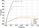
(1) Higgs Boson

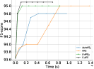
(2) A. Employee

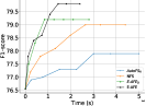
(3) PimaIndian

(4) SpectF

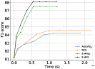
(5) SVMGuide3

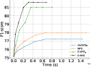
(6) German Credit

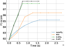
(7) AP. ovary

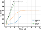
(8) Lymphography

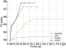
(9) Ionoshpere

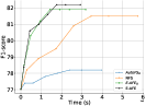
(10) Credit Default

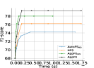
(11) Messidor features

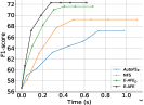
(12) Wine Q. Red

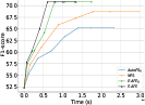
(13) Wine Q. White

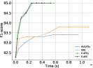
(14) SpamBase

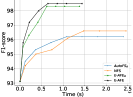
(15) AP. lung

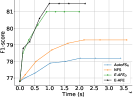
(16) credit-a

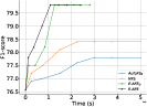
(17) diabetes

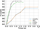
(18) fertility

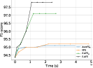
(19) gisette

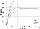
(20) hepatitis

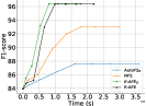
(21) labor

(22) lymph

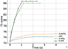
(23) madelon

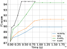
(24) megawatt1

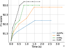
(25) secom

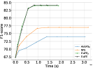
(26) sonar

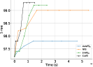
(27) Bikeshare DC

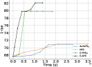
(28) Housing Boston

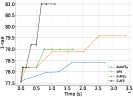
(29) Airfoil

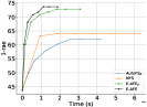
(30) Openml 618

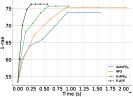
(31) Openml 589

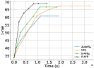
(32) Openml 616

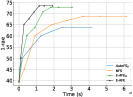
(33) Openml 607

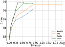
(34) Openml 620

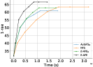
(35) Openml 637

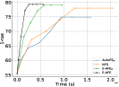
(36) Openml 586

Figure 7: Performance comparison. We show the converging curve of four methods on target datasets. E-AFE is our method. $\mathrm{AutoFS_{R}}$ [11, 12] is feature selection from randomly generated features. $\mathrm{NFS}$ [6] is feature generation and evaluation. $\emph{E-AFE}_{D}$ is the ablation study of  E-AFE , replacing the approximate hashing model with a random dropout method.

IV-E Comparison with DNN method (Q4)

To compare the feature engineering method with the deep learning method, we invite the RTDL [10] method for baseline.

In Table III, we can see that feature engineering-related methods are more robust than ResNet from RTDL. The results of ResNet have 0.0 or near 0.0. We consider that ResNet is less useful in mini datasets, such as Lymphography and hepatitis. In the mini dataset, NFS [6] and  E-AFE  have significant advantages to ResNet. However, if the dataset is large, ResNet performs similarly to NFS [6] and  E-AFE , such as Higgs Boson, SpamBase, AP. lung, and gisette. The robustness loss of DNN results comes from its pre-division of data sets into training, validation, and test sets. Especially for small data sets, this partition is a fatal disadvantage. The robust result comes from the cross-validation downstream task of the feature engineering-related method, though this cross-validation is very time-consuming. We also mix deep learning and feature engineering methods in Table III, and DL|FE and FE|DL also support the above analysis results.

IV-F Hyperparameter Sensitivity Studies (Q5)

E-AFE  involves several parameters (e.g., Threshold $thre$, MinHash signature output dimension and Maximum Order). To investigate the robustness of our method, we examine how the different choices of parameters affect the performance of  E-AFE . Except for the parameter being tested, we set other parameters at the default values.

We use auto-sklearn for training and validation the FPE model. $thre$ divides the features into positive and negative ones. The FPE model is trained on the approximate hashing features from the original public training set and validated on the approximate hashing features from the validation set.

Figure 8 shows the evaluation results on data as a function of one selected parameter when fixing others. Overall, we observe that  E-AFE  is not strictly sensitive to these parameters, demonstrating our proposed framework’s robustness. In particular, we can observe that score achieves better performance with the decrease of the threshold. The reason is that a smaller threshold has a larger recall for the validation set. The MinHash output length have something with the score. The reason is that the approximate features generated by the hash function can affect training results. This paper uses a variety of hash functions and different compressed feature lengths to generate approximate features. If the MinHash signature output dimension set is too small, it will extract too little information from the original feature and is not conducive to hash model training. Some datasets may get a better score with the maximum order increase, but the evaluated features and training time will increase significantly. Our experiments set the maximum order as 5 due to the effectiveness and computational cost trade-offs.

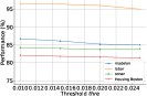
(1) Threshold $thre$.

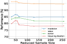
(2) MinHash signature output dimension .

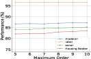
(3) Maximum Order.

Figure 8: Hyperparameter sensitivity studies of  E-AFE .

IV-G MinHash Explanations and Signature Sensitivity (Q6)

On the one hand, MinHash can map arbirtary size samples into the fixed size (like other Hash functions do), which is necessary for across datasets data engineering; on the other hand, one unique property of MinhHash is to quickly estimate the similarity between two samples with hashing signature, which can capture and preserve the relationships between samples during hashing, leading to limited information loss caused by compression [7]. Table III shows little difference in the effect obtained by different MinHash functions.

IV-H Replace downstream task (Q7)

TABLE V: Comparison results on 36 datasets. C is classification, R is regression. $\mathrm{AutoFS_{R}}$ [11, 12] is feature selection from randomly generated features. $\mathrm{NFS}$ [6] is feature generation and evaluation. SVM is support vector machines, NB is gaussian naive bayes for classification, GP is gaussian processes for regression, MLP is multi-layer perceptron.

Dataset C\R $\mathrm{AutoFS_{R}}$ NFS E-AFE SVM NB|GP MLP SVM NB|GP MLP SVM NB|GP MLP fertility C 0.880 0.670 0.760 0.870 0.140 0.300 0.880 0.880 0.900 hepatitis C 0.794 0.819 0.561 0.774 0.316 0.329 0.813 0.826 0.813 labor C 0.648 0.839 0.482 0.582 0.667 0.333 0.876 0.911 0.808 PimaIndian C 0.762 0.749 0.569 0.638 0.352 0.469 0.779 0.772 0.626 credit-a C 0.655 0.657 0.536 0.545 0.555 0.445 0.733 0.748 0.713 diabetes C 0.762 0.757 0.509 0.642 0.352 0.397 0.770 0.768 0.638 german credit C 0.713 0.727 0.663 0.688 0.302 0.390 0.734 0.754 0.731 ionosphere C 0.937 0.869 0.539 0.632 0.442 0.388 0.952 0.906 0.821 sonar C 0.558 0.590 0.518 0.447 0.441 0.335 0.683 0.667 0.721 spambase C 0.606 0.826 0.899 0.568 0.388 0.399 0.810 0.847 0.914 SPECTF267 C 0.790 0.670 0.701 0.775 0.513 0.323 0.839 0.794 0.798 AP. lung C 0.695 0.936 0.626 0.586 0.404 0.339 0.936 0.946 0.867 lymph C 0.899 0.935 0.682 0.499 0.456 0.363 0.928 0.950 0.884 lymphography C 0.810 0.713 0.570 0.563 0.465 0.352 0.852 0.838 0.768 madelon C 0.664 0.504 0.535 0.469 0.468 0.435 0.751 0.621 0.578 megawatt1 C 0.893 0.806 0.565 0.873 0.166 0.222 0.897 0.893 0.893 messidor features C 0.693 0.611 0.517 0.513 0.467 0.476 0.709 0.643 0.673 AP. ovary C 0.804 0.789 0.636 0.695 0.284 0.280 0.822 0.829 0.775 secom C 0.934 0.720 0.906 0.925 0.262 0.712 0.934 0.919 0.931 A. Employee C 0.942 0.912 0.890 0.942 0.746 0.683 0.942 0.942 0.942 svmguide3 C 0.762 0.817 0.763 0.749 0.240 0.314 0.817 0.825 0.778 Wine Q. Red C 0.511 0.528 0.475 0.425 0.459 0.334 0.537 0.553 0.527 Wine Q. White C 0.458 0.436 0.374 0.441 0.159 0.337 0.477 0.479 0.476 credit default C 0.779 0.380 0.660 0.778 0.222 0.492 0.808 0.780 0.777 gisette C 0.580 0.555 0.880 0.498 0.486 0.506 0.962 0.900 0.920 higgs boson C 0.704 0.685 0.695 0.669 0.331 0.432 0.735 0.701 0.720 Bikeshare DC R 0.977 0.773 0.998 0.976 0.773 0.998 0.977 0.773 0.999 boston housing R 0.614 0.468 0.509 0.612 0.467 0.476 0.614 0.468 0.525 Airfoil R 0.680 0.311 0.323 0.670 0.311 0.323 0.680 0.314 0.341 openml 618 R 0.631 0.523 0.218 0.630 0.523 0.438 0.633 0.523 0.671 openml 589 R 0.638 0.548 0.543 0.637 0.548 0.249 0.641 0.548 0.605 openml 616 R 0.552 0.486 0.324 0.549 0.486 0.459 0.558 0.486 0.636 openml 607 R 0.623 0.485 0.369 0.620 0.485 0.497 0.624 0.485 0.606 openml 620 R 0.619 0.521 0.340 0.618 0.518 0.488 0.622 0.521 0.265 openml 637 R 0.519 0.468 0.404 0.517 0.468 0.409 0.523 0.473 0.575 openml 586 R 0.647 0.523 0.756 0.646 0.523 0.726 0.649 0.523 0.759

We add one more experiment to verify that the features generated by our AFE are also robust to other downstream tasks. Specifically, we cache the features generated by different AFEs and replace Random Forest with other models (i.e., taking widely-used SVM as an exmaple) to evaluate the quality of these features. We also list the results in Table V for your reference. The results indicate that with our proposed framework, the features obtained from random forest can consistently outperform baselines using SVM, which indicates the features selected by our method are robust to other models.

IV-I Improvement analysis (Q8)

TABLE VI: P-value of  E-AFE  with other baseline methods

P-value $AutoFS_{R}$| E-AFE $RTDL_{N}$ | E-AFE NFS | E-AFE Performance $5.08\times 10^{-2}$ $9.87\times 10^{-7}$ $1.83\times 10^{-1}$ Time $1.97\times 10^{-6}$ $2.75\times 10^{-11}$ $3.75\times 10^{-6}$

Specifically, we calculate the $p-value$ of the improvement over each baseline method in terms of both effectiveness (accuracy) and efficiency (running time) to check the significance. The results in Table VI indicate that for efficiency, $p-value$ of improvement over baselines NFS, $AutoFS_{R}$, and $RTDL_{N}$ are $3.75\times 10^{-6}$, $1.97\times 10^{-11}$, and $2.75\times 10^{-11}$, respectively, which shows that the improvement on efficiency is statistically significant; for effectiveness, the improvement over $RTDL_{N}$ is statistically significant with $p-value$ as $9.87\times 10^{-7}$, and the improvement over $AutoFS_{R}$ is statistically near-significant with $p-value$ as $5.08\times 10^{-2}$. But the effectiveness improvement over NFS is not statistically significant with the $p-value$ as $1.83\times 10^{-1}$. The reason is that the difference of our method over NFS is mainly on developing the two-stage training strategy with reduced sample/feature size to improve the efficiency, while both of the two methods exploits reinforcement learning-based cross-validation for feature evaluation. Thus, the improvement on efficiency is statistically significant, while the effectiveness improvement is incremental.

IV-J Scalability analysis (Q9)

(1) Performance vs. Feature Number

(2) Performance vs. Sample Number

(3) Performance vs. Feature Number

(4) Performance vs. Sample Number

Figure 9: Time or performance improvement vs. feature or sample size.

Figure 9 results show the relationship between running time and performance improvement with data size. The performance improvement of E-AFE on larger datasets are better on smaller dataset, which demonstrate scalability ability of our proposed method.

V Related Work

V-A Automated Feature Engineering

AFE method can be divided into three types: (1)The downstream task has no feedback to the feature generator. ExploreKit [19] performs all transformation functions on the dataset. AutoLearn [2] preprocesses raw features and discards features with low information gain. Learning Feature Engineering (LFE) [4] uses feature-class representation and a set of Multi-Layer Perception (MLP) classifiers to predict whether the transformation result is better than the original feature. (2)The downstream task gives feedback to the feature generator with RL. Transformation Graph [5] builds DAG and uses Q-learning to exploit high-order features. Neural Feature Search (NFS) [6] predicts the most appropriate transformation for each feature by policy gradient for better feature generation. Group-wise Reinforcement Feature Generation (GRFG) [20] proposes a principled framework to address the automation, explicitness, optimal issues in representation space reconstruction. (3)Feature selection with RL ignores feature generation. Multi-Agent Reinforcement Learning Feature Selection (MARLFS), Interactive Reinforced Feature Selection (IRFS), Single-Agent Reinforcement Learning Framework (SADRLFS), Monte Carlo based reinforced feature selection (MCRFS), Group-based Interactive Reinforced Feature Selection (GIRFS) and Combinatorial Multi-Armed Bandit (CMAB) on feature selection [21, 11, 22, 12, 23, 24, 25, 26] use RL in feature selection. However, those RL frameworks can’t consider feature generation.

V-B Approximate Feature

To speed up feature engineering, many methods to obtain an approximate dataset from the original dataset are proposed. We summarize four classes of approximate feature methods. (1)Meta-Feature. Previous approaches used hand-crafted meta-features, including information-theoretic and statistical meta-features, to represent datasets [27, 28, 29, 19]. Meta-Feature Extractor (MFE) [30, 31] extracts meta-features from the dataset to improve the reproducibility of machine learning. Automatic generation of meta-features [32] presents a framework to generate meta-features in the context of meta-learning systematically. ExploreKit [19] generates two types of meta-features: dataset-based and candidate features-based. (2)Low-rank matrix approximation [33, 34] finds a smaller rank matrix similar to the original matrix. (3)Quantile Data Sketch was used in LFE [4] to represent feature values. (4)Hashing method. Feature Hashing [35] introduces specialized hash functions with unbiased inner products that are directly applicable to a large variety of kernel methods. Hash kennel [36, 37] computes the kernel matrix for data streams and sparse feature spaces.

VI Conclusion Remarks

In this paper, we studied how to improve the efficiency of AFE. Based on the empirical studies, we identified that the time-consuming feature evaluation procedure is the core reason of interfering with AFE’s running efficiency. We further validated that smaller sample size and feature size would accelerate feature evaluation. Therefore, we proposed to improve the efficiency of AFE by reducing the sample and feature size. Specifically, we develop FPE model, including a sample compressor with MinHash to reduce sample size , and a feature pre-selector with a pre-trained binary classifier to distinguish the effectiveness of the generated features. Moreover, we devised a two-stage training strategy to first initialize the policy using the binary feature-effectiveness classification as the evaluation task to borrow external knowledge from the pre-trained FPE. The enhanced initialization provideed the AFE policy with a good starting point for exploring the optimal actions, which further significantly save the running time. Finally, we conduct extensive experiments on 36 datasets on both the classification and regression tasks. When compared to state-of-the-art AFE methods, the results show 2.9 percent higher average performance and 2x higher computational efficiency. The improvements over both the effectiveness and efficiency proved that FPE model can remove the redundancy in candidate features.

VII Acknowledgements

This paper is jointly funded by National Key R&D Program of China (No. 2019YFB2102100), The Science and Technology Development Fund of Macau SAR (File no. 0015/2019/AKP), Key-Area Research and Development Program of Guangdong Province (NO.2020B010164003), GuangDong Basic and Applied Basic Research Foundation (No. 2020B1515130004), The Science and Technology Development Fund, Macau SAR (File no. SKL-IOTSC-2021-2023 to Chengzhong Xu and Pengyang Wang), and The Start-up Research Grant of University of Macau (File no. SRG2021-00017-IOTSC to Pengyang Wang).

References

- [1] Q. Shi, Y.-L. Zhang, L. Li, X. Yang, M. Li, and J. Zhou, “Safe: Scalable automatic feature engineering framework for industrial tasks,” in 2020 IEEE 36th International Conference on Data Engineering (ICDE). IEEE, 2020, pp. 1645–1656.
- [2] A. Kaul, S. Maheshwary, and V. Pudi, “Autolearn—automated feature generation and selection,” in 2017 IEEE International Conference on data mining (ICDM). IEEE, 2017, pp. 217–226.
- [3] L. Kotthoff, C. Thornton, H. H. Hoos, F. Hutter, and K. Leyton-Brown, “Auto-weka: Automatic model selection and hyperparameter optimization in weka,” in AUTOMATED MACHINE LEARNING: METHODS, SYSTEMS, CHALLENGES. Springer, Cham, 2019, pp. 81–95.
- [4] F. Nargesian, H. Samulowitz, U. Khurana, E. B. Khalil, and D. S. Turaga, “Learning feature engineering for classification.” in IJCAI, 2017, pp. 2529–2535.
- [5] U. Khurana, H. Samulowitz, and D. Turaga, “Feature engineering for predictive modeling using reinforcement learning,” in Proceedings of the AAAI Conference on Artificial Intelligence, vol. 32, no. 1, 2018.
- [6] X. Chen, Q. Lin, C. Luo, X. Li, H. Zhang, Y. Xu, Y. Dang, K. Sui, X. Zhang, B. Qiao et al., “Neural feature search: A neural architecture for automated feature engineering,” in 2019 IEEE International Conference on Data Mining (ICDM). IEEE, 2019, pp. 71–80.
- [7] W. Wu, B. Li, L. Chen, J. Gao, and C. Zhang, “A review for weighted minhash algorithms,” IEEE Transactions on Knowledge and Data Engineering, 2020.
- [8] J. R. Williams, “Simple statistical gradient-following algorithms for connectionist reinforcement learning,” Machine Learning, pp. 229–256, 1992.
- [9] P. C. Robert and G. Casella, “Monte carlo statistical methods,” Monte Carlo Statistical Methods, 2010.
- [10] Y. Gorishniy, I. Rubachev, V. Khrulkov, and A. Babenko, “Revisiting deep learning models for tabular data,” NeurIPS 2021, 2021.
- [11] W. Fan, K. Liu, H. Liu, P. Wang, Y. Ge, and Y. Fu, “Autofs: Automated feature selection via diversity-aware interactive reinforcement learning,” 20TH IEEE INTERNATIONAL CONFERENCE ON DATA MINING (ICDM 2020), pp. 1008–1013, 2020.
- [12] W. Fan, K. Liu, H. Liu, Y. Ge, H. Xiong, and Y. Fu, “Interactive reinforcement learning for feature selection with decision tree in the loop,” IEEE Transactions on Knowledge and Data Engineering, 2021.
- [13] W. Wu, B. Li, L. Chen, and C. Zhang, “Consistent weighted sampling made more practical,” in Proceedings of the 26th International Conference on World Wide Web, 2017, pp. 1035–1043.
- [14] S. Ioffe, “Improved consistent sampling, weighted minhash and l1 sketching,” Data Mining, pp. 246–255, 2010.
- [15] P. Li, “0-bit consistent weighted sampling,” ACM Knowledge Discovery and Data Mining, pp. 665–674, 2015.
- [16] W. Wu, B. Li, L. Chen, and C. Zhang, “Canonical consistent weighted sampling for real-value weighted min-hash,” 2016 IEEE 16TH INTERNATIONAL CONFERENCE ON DATA MINING (ICDM), pp. 1287–1292, 2016.
- [17] k. he, x. zhang, s. ren, and j. sun, “Deep residual learning for image recognition,” 2016 IEEE CONFERENCE ON COMPUTER VISION AND PATTERN RECOGNITION (CVPR), pp. 770–778, 2016.
- [18] D. P. Kingma and J. Ba, “Adam: A method for stochastic optimization,” arXiv preprint arXiv:1412.6980, 2014.
- [19] G. Katz, C. R. E. Shin, and D. Song, “Explorekit: Automatic feature generation and selection,” 2016 IEEE 16TH INTERNATIONAL CONFERENCE ON DATA MINING (ICDM), pp. 979–984, 2016.
- [20] D. Wang, Y. Fu, K. Liu, X. Li, and Y. Solihin, “Group-wise reinforcement feature generation for optimal and explainable representation space reconstruction,” arXiv preprint arXiv:2205.14526, 2022.
- [21] K. Liu, Y. Fu, P. Wang, L. Wu, R. Bo, and X. Li, “Automating feature subspace exploration via multi-agent reinforcement learning,” ACM SIGKDD, pp. 207–215, 2019.
- [22] K. Liu, Y. Fu, L. Wu, X. Li, C. Aggarwal, and H. Xiong, “Automated feature selection: A reinforcement learning perspective,” IEEE Transactions on Knowledge and Data Engineering, 2021.
- [23] X. Zhao, K. Liu, W. Fan, L. Jiang, X. Zhao, M. Yin, and Y. Fu, “Simplifying reinforced feature selection via restructured choice strategy of single agent,” 20TH IEEE INTERNATIONAL CONFERENCE ON DATA MINING (ICDM 2020), pp. 871–880, 2020.
- [24] K. Liu, P. Wang, D. Wang, W. Du, O. D. Wu, and Y. Fu, “Efficient reinforced feature selection via early stopping traverse strategy,” 2021 IEEE International Conference on Data Mining (ICDM), pp. 399–408, 2021.
- [25] W. Fan, K. Liu, H. Liu, A. Hariri, D. Dou, and Y. Fu, “Autogfs: Automated group-based feature selection via interactive reinforcement learning,” in Proceedings of the 2021 SIAM International Conference on Data Mining (SDM). SIAM, 2021, pp. 342–350.
- [26] K. Liu, H. Huang, W. Zhang, A. Hariri, Y. Fu, and K. Hua, “Multi-armed bandit based feature selection,” in Proceedings of the 2021 SIAM International Conference on Data Mining (SDM). SIAM, 2021, pp. 316–323.
- [27] D. Michie, J. D. Spiegelhalter, C. C. Taylor, and J. Campbell, “Machine learning, neural and statistical classification,” Technometrics, 1995.
- [28] a. kalousis and H. M., “Model selection via meta-learning: a comparative study,” International Journal on Artificial Intelligence Tools, pp. 525–554, 2001.
- [29] M. Feurer, A. Klein, K. Eggensperger, T. J. Springenberg, M. Blum, and F. Hutter, “Efficient and robust automated machine learning,” Annual Conference on Neural Information Processing Systems, pp. 2962–2970, 2015.
- [30] A. Rivolli, P. F. L. Garcia, C. Soares, J. Vanschoren, and C. P. L. F. d. A. Carvalho, “Towards reproducible empirical research in meta-learning,” arXiv: Learning, 2018.
- [31] E. Alcobaça, F. Siqueira, A. Rivolli, L. P. F. Garcia, J. T. Oliva, A. C. de Carvalho et al., “Mfe: Towards reproducible meta-feature extraction.” J. Mach. Learn. Res., vol. 21, pp. 111–1, 2020.
- [32] F. Pinto, C. Soares, and J. Mendes-Moreira, “Towards automatic generation of metafeatures,” ADVANCES IN KNOWLEDGE DISCOVERY AND DATA MINING, PAKDD 2016, PT I, pp. 215–226, 2016.
- [33] M. A. Frieze, R. Kannan, and S. Vempala, “Fast monte-carlo algorithms for finding low-rank approximations,” Journal of the ACM (JACM), pp. 1025–1041, 2004.
- [34] H. N. Nguyen, T. T. Do, and D. T. Tran, “A fast and efficient algorithm for low-rank approximation of a matrix,” STOC, pp. 215–224, 2009.
- [35] Q. K. Weinberger, A. Dasgupta, J. Langford, J. A. Smola, and J. Attenberg, “Feature hashing for large scale multitask learning,” international conference on machine learning, pp. 1113–1120, 2009.
- [36] Q. Shi, J. Petterson, G. Dror, J. Langford, J. A. Smola, L. A. Strehl, and S. V. V. N, “Hash kernels,” AISTATS, pp. 496–503, 2009.
- [37] Q. Shi, J. Petterson, G. Dror, J. Langford, A. Smola, and S. Vishwanathan, “Hash kernels for structured data,” Journal of Machine Learning Research, pp. 2615–2637, 2009.