Semantic Enhanced Knowledge Graph for Large-Scale Zero-Shot Learning

Abstract

Zero-Shot Learning has been a highlighted research topic in both vision and language areas. Recently, most existing methods adopt structured knowledge information to model explicit correlations among categories and use deep graph convolutional network to propagate information between different categories. However, it is difficult to add new categories to existing structured knowledge graph, and deep graph convolutional network suffers from over-smoothing problem. In this paper, we provide a new semantic enhanced knowledge graph that contains both expert knowledge and categories semantic correlation. Our semantic enhanced knowledge graph can further enhance the correlations among categories and make it easy to absorb new categories. To propagate information on the knowledge graph, we propose a novel Residual Graph Convolutional Network (ResGCN), which can effectively alleviate the problem of over-smoothing. Experiments conducted on the widely used large-scale ImageNet-21K dataset and AWA2 dataset show the effectiveness of our method, and establish a new state-of-the-art on zero-shot learning. Moreover, our results on the large-scale ImageNet-21K with various feature extraction networks show that our method has better generalization and robustness.

I Introduction

Recently, with the fast development of deep learning techniques [19, 55, 2, 3, 4, 5] and large-scale high-quality annotated datasets [30], visual object recognition has made remarkable achievements. However, to obtain a good multi-class classifier, thousands of high-quality labeled images are needed to train the model, the learned classifier can only identify the categories that participate in the training. In real-world applications, there are tens of thousands of categories, most of which are long tail. It is laboriously to collect and label large amounts of data for each category. Moreover, new categories are emerging endlessly, it is also difficult to collect sufficient training data for these new categories. Therefore, how to develop a robust algorithm for classification in the case of limited samples or even zero samples is a very urgent and arduous task.

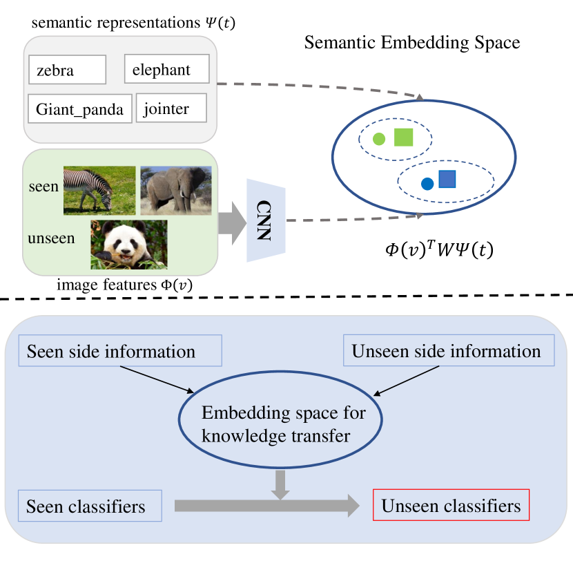
Figure 1: Illustration of the semantic embedding-based (top) and the classifiers-based (bottom) methods that are typically used for zero-shot learning.

To address such issues, Zero-Shot Learning (ZSL) [82, 59, 83, 49, 81, 79, 78, 80, 76, 52, 59, 51, 65, 60, 61, 62, 63, 64] has recently attracted great attention, which aims to recognize new categories without any exemplars. The core idea of ZSL is to emulate the intelligence of humans in transfering knowledge obtained from seen categories to describe the unseen categories. Existing ZSL methods can be divided into two paradigms: (1) embedding-based. Embedding-based [44, 6, 20] methods learn a projection from visual space to semantic (e.g., attribute or word embedding) space based on the dataset of seen categories. In such a setting, an effective common embedding space is constructed to associate seen categories and unseen categories for knowledge transfer. (2) classifier-based. Classifier-based methods [58, 24, 15] learn a classifier for new categories. The core idea behind these methods is to use semantic information (e.g., word embedding) to model correlations among seen and unseen categories in semantic space, and learn a classifier for unseen categories. As illustrated in Figure. 1.

Embedding-based methods have a general hypothesis that a projection function existing in semantic space measures the compatibility between the visual features and the side information for both seen and unseen categories [1]. During training, a mapping matrix is learned from the labeled data. At test phase, the learned mapping matrix is shared between the seen and unseen categories, so unlabeled data can be accurately identified by resorting to the nearest neighbor search in the common semantic space. In the last decade, many regularization terms and various optimization objectives have been extensively studied to obtain better mapping matrix.

The alternative and less-explored paradigm is to generate a classifier for novel categories based on the explicit or implicit correlations among seen and unseen categories. In this paradigm, the key issue is to model the correlations among seen and unseen categories. Li et al. [8] learned simple linear semantic correlations among seen and unseen category prototypes, and generated a classifier for unseen categories based on the learned semantic correlations. Misra et al. [9] generated classifiers for complex visual concepts by composing simple concepts primitives classifiers. However, the correlations among different categories can be more complex than a linear combination. Moreover, the above methods only explored the correlations among categories in an implicit way.

Recently, some studies have used structured knowledge information (knowledge graph) to model explicit correlations among categories, and achieved favorable performance in various computer vision tasks such as zero-shot action recognition [10, 72], multi-label image classification [11, 12], cross-modal retrieval [74, 75, 59], object detection [13], etc. The great advantage of knowledge graph is that it allows statistical strength to be shared between related categories. Due to the particular structure of the knowledge graph, to effectively utilize the knowledge information in the knowledge graph, Graph Convolutional Networks (GCN) [14, 73] is used to propagate information among different categories. Wang et al. [15] designed a 6-layer deep GCN for zero-shot recognition.

However, deep GCN suffers from over-smoothing problem. In recent work, Li et al. [17] demonstrated that GCN performs a form of Laplacian smoothing. As the number of GCN layers increases, the node features may be over-smoothed so that node features from different categories may become indistinguishable [12]. To alleviate the problem of over-smoothing caused by deep GCN, we design a novel Residual Graph Convolutional Network (ResGCN) for ZSL by introducing residual connections into the hidden layer of GCN. Veit et al. [18] proved that the residual networks [19] can be viewed as an ensemble of shallow networks. Residual Graph Convolutional Network has the same merit with residual networks and can effectively alleviate over-smoothing.

Furthermore, existing knowledge graph-based methods directly extract fixed relationships from WordNet [16], which limits the scalability of knowledge graphs. Since WordNet is built by experts, it is difficult to absorb new categories. To address this problem, we propose a new method to build a Semantic Enhanced Knowledge Graph (SE-KG) that contains both expert knowledge and semantic information. In practice, the word embeddings of related categories are close to each other in the semantic space. Therefore, if the word embeddings are close to each other in the semantic space, their corresponding categories should have edges connected in the knowledge graph. Concretely, we first build a basic knowledge graph from WordNet, and then connect the categories whose word embeddings are close to each other in the semantic space. For a new category that is not in WordNet, it can be absorbed by connecting it with the semantically closer category in the knowledge graph.

Most existing zero-shot methods are well designed and can achieve competitive results on small datasets. However, their performance degrades rapidly on the large-scale datasets, such as ImageNet-21K [30]. One possible reason could be that these methods learned an ambiguous inter-class relationship to transfer knowledge. As the number of unseen categories increases, the drawback of these methods become more serious. Furthermore, one major shortcoming of small datasets is that the number of unseen categories is dwarfed by the number of seen categories. To solve such issues, we provide a new method that focuses on the large-scale zero-shot image classification. We evaluate our method mainly on the large-scale ImageNet-21K dataset. For generalization, we also report experimental results on the AWA2 [49] dataset.

The main contributions of this paper are summarized as follows:

• We design a novel Residual Graph Convolutional Network (ResGCN) for ZSL, which can effectively alleviate the problem of over-smoothing in GCN based models.

• We present a new method to build a semantic enhanced knowledge graph that contains both expert knowledge and semantic information. Our method can further enhance the correlations among categories and easily absorb new categories into the knowledge graph.

• We conduct extensive experiments and evaluate our method on two widely used benchmarks, AWA2 and large-scale ImageNet-21K datasets. Experimental results show the effectiveness of our method.

• We show that our method can be easily applied to various feature extractor architectures and has better generalization and robustness.

This paper provides a more comprehensive development of the previous work [58], with more analysis, insights and evaluation. Compared to the previous work [58], (1) we have strengthened the introduction of our work. In particular, we have elaborated more details about the motivation of researching on zero-shot learning and the drawback of existing work in this field. (2) in Section III-C, we provide two new variants of residual convolutional networks to further improve performance. In the previous work [58], our residual block only skipping two layers. Noted that shallow GCN may limit representation abilities. To handle this problem, we provide two new variants of residual GCN with more skipping layers. (3) the experiment part is re-designed. More comparison methods are added to comprehensively illustrate the superiority of our model. In Section IV, we provide in-depth analysis of experimental results. Specifically, (a) in Section IV-B, we evaluate our method on more datasets and achieve competitive results; (b) in Section IV-D, we provide Qualitative Results; (c) in Section IV-E, we provide Ablation Study with more experimental setting. Furthermore, we apply our method to various architectures. Experimental results show that the proposed method has better generalization and robustness.

The rest of this paper is organized as follows. Section II provides a review of related work. In Section III, we elaborate on the proposed residual graph convolution network and semantic enhanced knowledge graph. In Section IV, we test our method on the two benchmarks. The conclusion is presented in Section V.

II Related Work

In this section, we review related work on the study of zero-shot learning. Existing methods are divided into two categories: embedding-based and classifier-based.

Embedding-based methods. Most previous work introduced linear or nonlinear modeling methods to learn a mapping matrix for zero-shot learning. Generality, these methods have two stages: firstly, learn a mapping matrix between visual features and side information (e.g., attribute, word embedding) on the training dataset; secondly, predict the test samples by performing the nearest neighbor search in the common embedding space. Attributes which defined as various properties of categories are widely used in early ZSL work. Lampert et al. [20] proposed a method named Direct Attributes Prediction (DAP), which infers the attributes of an image for the first time. Li et al. [1] proposed a method to learn discriminative semantic representations in an augmented space for attributes. However, the manually-defined attributes are subjective, and attributes annotation are difficult and laborious.

As an alternative, word embeddings have been widely studied for ZSL. Word embeddings are learned from a large linguistic corpora [6], each category can be uniquely represented by a word embedding vector in the word embedding space. Socher et al. [6] proposed a non-linear model to project visual features into the word embedding space. Frome et al. [7] designed a linear transformation layer to measure the compatibility between the visual features and word embeddings. In order to explore the complementary of different semantic information, Ji et al. [21] proposed a model named Multi-Battery Factor Analysis (MBFA), which constructed a unified semantic space for both visual features and multiple types of semantic information. Instead of learning a projection function between visual features and semantic information, Changpingyo et al. [22] proposed a kernel-based method to learn an exemplar for each category through semantic representation. Norouzi et al. [23] directly generated a semantic vector for each unseen category via a convex combination of seen categories word embeddings. Above methods all adopt the semantic space as a bridge to measure the compatibility between the visual features and the semantic information, however, the generalization capabilities of semantic models and mapping models are limited, resulting in poor performance of these methods.

Classifiers-based methods. Recently, there are many methods to learn a classifier for each new category. The core idea behind these methods is to mine correlations among categories and generate classifiers for new categories based on this correlation. Li et al. [8] proposed a model to learn the correlations among seen and unseen prototypes, thus the unseen classifiers can be generated by combinations of seen classifiers using the same correlations. Changpinyo et al. [24] proposed a method to synthesize classifiers for unseen categories via aligning the semantic space and visual space. Nevertheless, the above approaches only mine the implicit correlations among categories. Another popular way to transfer knowledge is using knowledge graph to model the explicit correlations among categories. Marino et al. [11] proposed a graph search neural network and used knowledge graph for object recognition. Lee et al. [25] introduced a knowledge graph to model the correlations among multiple labels. One strong shortcoming of these methods is they did not incorporate unseen labels during training [10]. DGP [52] exploits the hierarchical structure of the knowledge graph by connecting the ancestors and descendants. Wang et al. [15] introduced a knowledge graph to model the explicit correlations among categories, and used a deep graph convolutional network to propagate message among different categories. However, this method is deficient since the knowledge graph they built only considers expert knowledge and ignores the labels semantic correlation. Moreover, deep graph convolutional network suffers from over-smoothing problem.

To address such issues, we introduce a new semantic enhanced knowledge graph (SE-KG) that contains both expert knowledge and labels semantic correlation. In addition, we design a novel residual graph convolutional network to propagate messages among different categories in the new SE-KG. The proposed residual graph convolutional network can effectively alleviate over-smoothing problem.

III Proposed Method

III-A Problem Statement

Assume that there is a labeled source dataset $S={\{(\mathbf{x_{i}},y_{i})\}}_{i=1}^{ms}$, where $\mathbf{x_{i}}$ denoted as the visual feature vector, and each $\mathbf{x_{i}}$ is associated with a label $y_{i}$. There are $N_{s}$ distinct categories available for source dataset, ${y_{i}}\in Y_{s}=\{1,2,3,...,N_{s}\}$. In addition, there is a target dataset $T={\{({\mathbf{x_{j}}}\prime,{y_{j}}\prime)\}}_{i=1}^{mt}$, where $\mathbf{x_{j}}\prime$ denoted as visual feature vector, while ${y_{j}}\prime\in Y_{t}=\{N_{s}+1,\cdots,N_{s}+N_{t}\}$. Target dataset contains $N_{t}$ distinct categories, which are disjoint with source target, $Y_{s}\cap Y_{t}=\emptyset$. In general, the categories within source dataset are also referred to as the seen categories, the categories within target dataset are referred to as the unseen categories. Zero-shot learning aims to learn a classifier $(F:\mathbf{x_{i}}\to y_{i})$ on the $S$, which performs well on the target dataset $T$ $(F:{\mathbf{x_{j}}}\prime\to{y_{j}}\prime)$. Zero-shot learning is a non-trivial task, but it is infeasible without any side information. To mitigate zero-shot learning, in this paper, we formulated zero-shot learning as a classifier weights regression problem. Concretely, we associate each label with a word embedding, and learn a projection from word embedding to visual classifier for both seen and unseen categories.

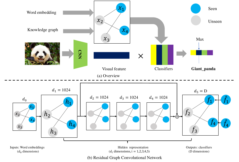
Figure 2: Example of a Residual Graph Convolutional Network for zero-shot learning. The input is the matrix of word embeddings and outputs are classifiers for each category. The ground-truth $\hat{\mathbf{f}_{1}}$ is extracted from the pre-trained CNN. During testing, with the classifiers predicted by our model, the inner product of the classifiers and the visual feature can be obtained, the classification is performed by ranking the value of the inner product.

III-B Graph Convolutional Network

Graph Convolutional Network (GCN) [14] aims to semi-supervised learning on graph-structured data. The key idea is to propagate message between different nodes via explicit graph-based correlations among categories. In semi-supervised setting, given an undirected graph that models the explicit correlations among different entities, where each node represents an entity and related entities are connected by edges. GCN takes nodes feature matrix $\mathcal{H}^{l}\in\mathbb{R}^{N\times d}$ and adjacency matrix $\mathcal{A}\in\mathbb{R}^{N\times N}$ (binary or weighted) as inputs, and updates the nodes feature as $\mathcal{H}^{l+1}\in\mathbb{R}^{N\times m}$, here $\mathcal{H}^{l}\in\mathbb{R}^{N\times d}$ is the hidden representation of the $l$-th layer, $N$ represents the number of nodes, and $d$ denotes the dimension of node features. Formally, layer-wise propagation rule in GCN can be defined as follows:

$$\mathcal{H}^{l+1}=\boldsymbol{\sigma}(\hat{\mathcal{A}}\mathcal{H}^{l}\mathcal{W}^{l}),$$ (1)

where $\hat{\mathcal{A}}\in\mathbb{R}^{N\times N}$ is the normalized version of adjacency matrix $\mathcal{A}$. $\boldsymbol{\sigma}(\cdot)$ denotes a nonlinear activation function. $\mathcal{W}^{l}\in\mathbb{R}^{d\times m}$ are the parameters of the $l$-th layer.

III-C Residual Graph Convolutional Network for ZSL

A deep GCN can be obtained by stacking multiple graph convolutional layers of the form of Eq. 1. In recent work, Li et al. [17] demonstrated that GCN performs a form of Laplacian smoothing. As the number of GCN layers increases, node features from different categories may become indistinguishable [12] due to over-smoothing. To address this issue, we explore introducing residual connections into GCN. Our work is inspired by residual networks [19]. More recently, Veit et al. [18] proved that the residual networks [19] can be viewed as an ensemble of shallow networks, deep convolutional networks can benefit by introducing residual connections. Residual Graph Convolutional Network has the same merit with residual networks [19] and can effectively alleviate over-smoothing.

TABLE I: Detailed architectures for the task of ZSL. “Identity” means that the identity shortcut is used. “Projection” means using the projection shortcut to match the dimension. D represents the dimension of the ground-truth classifier.

Layer name	Model-1	Model-2	Model-3	Model-4	Model-5
First layer	1024	2048	2048	1024	1024
Residual Connections	(Identity) 1024	(Projection) 2048 1024	(Identity) 2048 2048	(Identity) 1024 1024 1024	(Identity) 1024 2048 1024
	(Projection) 2048	(Identity) 1024 1024	(Projection) 2048 1024
Last layer	D	D	D	D	D

Similar to the residual networks [19], we introduce residual connections to every few stacked GCN layers. There are two forms of residual connections: identity shortcuts and projection shortcuts. For clarity of notation, we use function $F(\cdot)$ to encode a few stacked GCN layers, $F(\cdot)$ in this paper has one, two or three GCN layers. Identity shortcuts can be formulated as follows:

$$\mathcal{X}_{out}=F(\mathcal{X}_{in},\hat{\mathcal{A}},\{\mathcal{W}_{i}\})+\mathcal{X}_{in},$$ (2)

where $\hat{\mathcal{A}}$ is the normalized version of adjacency matrix $\mathcal{A}$, ${\mathcal{W}_{i}}$ are the parameters need to be learned, $\mathcal{X}_{in}$ and $\mathcal{X}_{out}$ are the input and output nodes feature matrix of the GCN layers considered. Note that $\mathcal{X}_{in}$ and $F(\mathcal{X}_{in},\hat{\mathcal{A}},\{\mathcal{W}_{i}\})$ have the same dimension. The operation $F(\mathcal{X}_{in},\hat{\mathcal{A}},\{\mathcal{W}_{i}\})+\mathcal{X}_{in}$ is performed by element-wise addition.

Projection shortcuts are used for case where the dimensions of $\mathcal{X}_{in}$ and $\mathcal{X}_{out}$ are not same, in which a linear projection is performed to match the dimensions. Projection shortcuts can be defined as:

$$\mathcal{X}_{out}=F(\mathcal{\mathcal{X}}_{in},\hat{\mathcal{A}},\{\mathcal{W}_{i}\})+(\hat{\mathcal{A}}\mathcal{X}_{in}\mathcal{W}_{j}),$$ (3)

where $\mathcal{W}_{j}$ is the parameter need to be learned. Note that the dimensions of ${(\hat{\mathcal{A}}\mathcal{X}}_{in}\mathcal{W}_{j})$ and $F(\mathcal{X}_{in},\hat{\mathcal{A}},\{\mathcal{W}_{i}\})$ are same.

Based on the above two forms of residual connections, we can design a residual graph convolutional network. Concretely, the identity shortcuts are used when the input and output have the same dimension. If not the case, the projection shortcuts are performed to match the dimensions. We have designed various residual graph convolutional networks for ZSL. One of our architectures is illustrated in Figure. 2, various detailed architectures are presented in Table I. Model 1 is designed to verify the effectiveness of single-skip. Models 2 and 3 are designed to verify whether hidden layer dimensions have an impact on model performance. However, shallow GCN in the residual block may limit representation abilities. To handle this problem, we provide two new variant networks, models 4 and 5, with more skipping GCN layers. Through comparative experiments, we can obtain the best architecture for ZSL. Note that model 4 is selected for subsequent experiments. More experimental results are presented in Section IV-E.

In this paper, we formulated zero-shot learning as a classifier weights regression problem. Concretely, we associate each label with a word embedding, and learn a projection from word embedding to visual classifier for both seen and unseen categories. For clarity of notation, given a dataset with $N$ categories, $S_{D}={\{(\mathbf{p}_{i},\mathbf{f}_{i})\}}_{i=1}^{N}$, where $\mathbf{p}_{i}$ represents the prototype of category $i$, and $\mathbf{f}_{i}$ denoted as the classifier weights. Note that each $\mathbf{p}_{i}$ is associated with a classifier $\mathbf{f}_{i}$, and $\mathbf{f}_{i}$ has the same dimension with visual features. In this paper, word embeddings are adopted as the prototypes of category. Specifically, $\mathbf{p}_{i}$ is known for all categories, and $\mathbf{f}_{i}$ is known for a subset of category. Let $S_{t}={\{(\mathbf{p}_{j},\hat{\mathbf{f}_{j}})\}}_{j=1}^{M}\in S_{D}$ be the set of training data. The goal of ZSL is to predict $\mathbf{f}_{i}$ for the remaining $N-M$ categories. During training, the input to our model is a matrix $\mathcal{P}={\{\mathbf{p}_{i}\}}_{i=1}^{N}$ of all category word embeddings, and the output is a set of visual classifiers ${F=\{\mathbf{f}_{i}\}}_{i=1}^{N}$. Formally, our model can be defined as follows:

$$F=\sigma(\cdots\sigma(\hat{\mathcal{A}}\mathcal{P}\mathcal{W}^{0})\cdots).$$ (4)

During training, we adopt the mean-square error loss to optimize the model.

$$Loss=\frac{1}{M}\sum_{j\in S_{t}}\mathit{MSE}(\mathbf{f}_{j},\hat{\mathbf{f}_{j}}),$$ (5)

here, $\mathbf{f}_{j}$ is the predicted classifier and $\hat{\mathbf{f}_{j}}$ is the ground-truth classifier which obtained from the top layer of a pre-trained ConvNet, such as ResNet-50. At test phase, we use the predicted classifiers to perform classification on the unseen category visual features. The predicted scores can be obtained by the Eq. 6:

$$y_{i}=\mathop{MAX}\limits_{\mathbf{f}_{j}\in F}\{{\mathbf{f}_{j}}^{T}\cdot\mathbf{x}_{i}\},$$ (6)

where $\mathbf{x}_{i}$ is the visual features extracted from a pre-trained ConvNet, and $y_{i}$ is the predicted label. Therefore, unseen categories can be accurately recognized without any exemplars in the training stage.

Input : WordNet knowledge graph, GloVe, $\alpha$, $k$

1: Extract the category name from WordNet;

2: Generate the word embedding for each category via GloVe;

3: Calculate the distance matrix of word embedding;

4: Select $k$ categories with the smallest distance from the current category for each category;

5: Delete neighbors with distance greater than $\alpha$;

6: Construct a $k$-NNG;

7: Calculate the adjacency matrix $\mathcal{B}$ of $k$-NNG;

8: Calculate the adjacency matrix $\mathcal{A}$ of WordNet knowledge graph;

9: Generate the adjacency matrix $\mathcal{C}$ of SE-KG, $\mathcal{C}=\mathcal{A}+\mathcal{B}$;

Output : Adjacency matrix $\mathcal{C}$ of SE-KG

Algorithm 1 The construction process of the SE-KG.

III-D Semantic Enhanced Knowledge Graph for ZSL

In practice, the word embeddings of related categories are close to each other in the semantic space. Therefore, if the word embeddings are close to each other in the semantic space, their corresponding categories should have edges connected in the knowledge graph. In fact, both expert knowledge and labels semantic correlation can contribute to the ZSL task either in a directly or indirectly way. To effectively use the correlations among categories, we introduce a new Semantic Enhanced Knowledge Graph (SE-KG) that contains both expert knowledge and labels semantic information.

In this section, we will elaborate on the proposed SE-KG. Firstly, we obtain a basic knowledge graph from WordNet, which contains expert knowledge. Let $\mathcal{A}$ be the adjacency matrix of the basic knowledge graph with self-connections. Secondly, generate the labels word embedding via a pre-trained language model (e.g., GloVe [26]), and construct a $k$-nearest neighbor graph ($k$-NNG) based on the distance of word embeddings. The $k$-nearest neighbor graph ($k$-NNG) is a graph in which two vertices $p$ and $q$ are connected by an edge, if the distance between $p$ and $q$ is among the $k$-th smallest distances from $p$ to other objects. Let $\mathcal{B}$ be the adjacency matrix of the $k$-NNG. Although other distance metrics are feasible, we use Euclidean distance in this paper. Finally, the adjacency matrix of the SE-KG can be obtained by adding the adjacency matrix of the basic knowledge graph and the adjacency matrix of $k$-NNG. Let $\mathcal{C}$ be the adjacency matrix of SE-KG, $\mathcal{C}=\mathcal{A}+\mathcal{B}$.

In practice, there are some categories weakly related to others, and their corresponding word embeddings are far away from the word embeddings of all other categories in the semantic space. To prevent these categories from being connected to their neighbor categories in the $k$-NNG, we set a threshold $\alpha$ for the distance. Concretely, for the nearest $k$ neighbor categories of a category, only the category whose distance is less than the threshold $\alpha$ will be connected to it in the $k$-NNG. Algorithm 1 gives the detailed algorithm for the SE-KG.

IV Experiments

IV-A Implementation Details

Datasets and Splits. In this section, we introduce the datasets and data splits used in this paper. The detailed data splits are summarized in Table II.

TABLE II: Datasets and splits.

Datasets	Subset	Seen	Unseen
ImageNet-21K	2-hops	1,000	1,549
	3-hops		7,860
	all		20,842
AWA2		40	10

ImageNet-21K. Most existing ZSL datasets have one major shortcoming is that the number of unseen categories is dwarfed by the number of seen categories. However, in practice, the number of unseen categories is much larger than the seen categories. To this end, we test our approach on the large-scale ImageNet-21K [30] dataset, which contains a total of 21,842 categories. In order to compare with existing state-of-the-art methods, we mirror the train/test split setting of [15, 7, 23]. Concretely, we train our model on the ImageNet 2012 1K dataset with 1,000 seen categories, and test on three datasets with increasing degree of difficulty. Three datasets are extracted from the large-scale ImageNet-21K dataset based on the semantic similarity to the training set labels. “2-hops” consists of roughly 1.5K categories, which within 2 tree hops of the ImageNet 2012 1K categories. “3-hops” consists of roughly 7.8K categories, which within 3 tree hops of the ImageNet 2012 1K labels. “All” includes all the ImageNet-21K labels. Noted that the labels in three datasets are disjoint with the ImageNet 2012 1K labels.

AWA2. AWA2 [49] is an extension version of the original Animals with Attributes dataset and contains 37,332 images of 50 categories. We following the data split in [49] to ensure that the test categories are disjoint with the ImageNet 2012 dataset. In [49], 40 categories are used for training and 10 for testing. Note that the AWA2 test categories are contained in the ImageNet-21K categories, we report result on the AWA2 by using the same approach with the ImageNet-21K dataset without extra training.

Zero-Shot Learning Settings. There are two zero-shot test settings: Conventional setting and Generalized setting. In conventional setting, at test phase, candidate categories being only unseen categories (without training labels); In generalized setting, candidate categories include both seen and unseen labels. Note that both conventional setting and generalized setting are tested on the same datasets, the difference is in the number of candidate labels. We report experimental results in both test settings.

TABLE III: Hit@k performance for the different models on ImageNet zero-shot learning task. Testing on unseen categories. $\ddagger$ indicated models without fine-tuning.

Test Set	Model	Reference	Hit@k (%)
			1	2	5	10	20
2-hops	ConSE [23]	ICLR2014	8.3	12.9	21.8	30.9	41.7
	SYNC [24]	CVPR2016	10.5	17.7	28.6	40.1	52.0
	PSR [77]	CVPR2018	9.4	-	26.3	-	-
	EXEM [22]	ICCV2017	12.5	19.5	32.3	43.7	55.2
	GCNZ [15]	CVPR2018	19.8	33.3	53.2	65.4	74.6
	DGP(-f)‡ [52]	CVPR2019	23.95	37.04	56.53	69.30	78.75
	Cacheux et al. [66]	ICCV2019	9.81	-	-	-	-
	Zhu et al. [69]	ICCV2019	11.0	-	-	-	-
	ResGCN	Ours	26.68	40.59	60.25	71.73	80.68
3-hops	ConSE [23]	ICLR2014	2.6	4.1	7.3	11.1	16.4
	SYNC [24]	CVPR2016	2.9	4.9	9.2	14.2	20.9
	PSR [77]	CVPR2018	2.8	-	4.8	-	-
	EXEM [22]	ICCV2017	3.6	5.9	10.7	16.1	23.1
	GCNZ [15]	CVPR2018	4.1	7.5	14.2	20.2	27.7
	DGP(-f)‡ [52]	CVPR2019	5.67	9.62	17.55	25.60	35.14
	Cacheux et al. [66]	ICCV2019	2.52	-	-	-	-
	Zhu et al. [69]	ICCV2019	2.40	-	-	-	-
	ResGCN	Ours	6.02	10.12	18.35	26.20	35.24
All	ConSE [23]	ICLR2014	1.3	2.1	3.8	5.8	8.7
	SYNC [24]	CVPR2016	1.4	2.4	4.5	7.1	10.9
	PSR [77]	CVPR2018	1.0	-	2.7	-	-
	EXEM [22]	ICCV2017	1.8	2.9	5.3	8.2	12.2
	GCNZ [15]	CVPR2018	1.8	3.3	6.3	9.1	12.7
	DGP(-f)‡ [52]	CVPR2018	2.65	4.54	8.42	12.71	18.38
	Cacheux et al. [66]	ICCV2019	1.09	-	-	-	-
	Zhu et al. [69]	ICCV2019	1.00	-	-	-	-
	ResGCN	Ours	2.78	4.74	8.76	12.86	18.46

Model Details. We adopt the GloVe [26] model trained on the Wikipedia dataset to obtain the word embeddings of labels. The dimension of word embeddings is set at 300. If category names contain multiple words, we obtain the category word embedding as average of embeddings for all words. For activation function, we adopt LeakyReLU [27] with the negative slope of 0.2. Following [15], we perform L2-Normalization on the predicted classifiers and ground-truth classifiers. For image representations, we adopt ResNeXt-101 pre-trained on the ImageNet 2012 1K dataset to generate the visual representations. For each image, the 2048-dimensional activations of the penultimate layer are taken as visual features. We also adopt the Dropout in each graph convolutional layer, with a dropout rate of 0.5. Different from [15], which performed symmetric normalization (Sym, $\hat{\mathcal{A}}=\mathcal{D}^{-\frac{1}{2}}\mathcal{A}\mathcal{D}^{-\frac{1}{2}}$) on adjacency matrix, we adopt a random walk normalization (Non-sym, $\hat{\mathcal{A}}=\mathcal{D}^{-1}\mathcal{A}$) on adjacency matrix. We train all architecture from scratch using Adam [28] with the initial learning rate is 0.001, and a weight decay 0.0005. The model is trained for 300 epochs in total. We implement our architecture by PyTorch [71].

TABLE IV: Top-1 results for unseen categories on AWA2. Results for ConSE, Devise and SYNC obtained from [49].

Model	Reference	Hit@1(%)
ConSE	ICLR2014	44.5
Devise	NeurIPS2013	59.7
SYNC	CVPR2016	46.6
Xian et al. [67]	CVPR2018	68.2
Cacheux et al. [66]	ICCV2019	67.9
GFZSL [68]	ECML2017	63.8
SE-GZSL [50]	CVPR2018	69.2
GCNZ	CVPR2018	70.7
ResGCN	Ours	77.4

IV-B Evaluation Results with Conventional Setting

Results on ImageNet-21K. We first contrast our approach to several existing state-of-the-art methods without considering the training labels. DeViSE [7] learned a linearly mapping matrix from visual space to word vector space. The model is initialized by two pre-trained neural network models, and trained by a hinge ranking loss. At test phase, an image is classified by comparing its similarity with the unseen categories in the semantic embedding space. Instead of learning a mapping matrix from visual space to semantic space, ConSE [23] directly generated a semantic embedding vector for an image in the semantic space through the convex combination of the top-$k$ likely train labels semantic embedding vectors. A test image is classified by comparing its embedding vector with unseen categories in the semantic embedding space.

TABLE V: Hit@k performance for the different models on ImageNet zero-shot learning task. Testing on both seen and unseen categories. $\ddagger$ indicated models without fine-tuning.

Test Set	Model	Reference	Hit@k (%)
			1	2	5	10	20
2-hops+1K	DeViSE [7]	NeurIPS2013	0.8	2.7	7.9	14.2	22.7
	ConSE [23]	ICLR2014	0.3	6.2	17.0	24.9	33.5
	PSR [77]	CVPR2018	1.2	-	11.2	-	-
	GCNZ [15]	CVPR2018	9.7	20.4	42.6	57.0	68.2
	DGP(-f)‡ [52]	CVPR2019	9.76	22.61	44.82	60.42	72.24
	FGZSL [67]	CVPR2018	4.40	-	-	-	-
	Zhu et al. [69]	ICCV2019	4.50	-	-	-	-
	ResGCN	Ours	10.80	25.47	50.41	64.44	75.22
3-hops+1K	DeViSE [7]	NeurIPS2013	0.5	1.4	3.4	5.9	9.7
	ConSE [23]	ICLR2014	0.2	2.2	5.9	9.7	14.3
	PSR [77]	CVPR2018	1.8	-	4.9	-	-
	GCNZ [15]	CVPR2018	2.2	5.1	11.9	18.0	25.6
	DGP(-f)‡ [52]	CVPR2019	2.81	6.07	14.37	22.72	32.73
	FGZSL [67]	CVPR2018	1.18	-	-	-	-
	Zhu et al. [69]	ICCV2019	1.20	-	-	-	-
	ResGCN	Ours	2.85	6.36	15.30	23.50	32.85
All+1K	DeViSE [7]	NeurIPS2013	0.3	0.8	1.9	3.2	5.3
	ConSE [23]	ICLR2014	0.2	1.2	3.0	5.0	7.5
	PSR [77]	CVPR2018	0.4	-	1.7	-	-
	GCNZ [15]	CVPR2018	1.0	2.3	5.3	8.1	11.7
	DGP(-f)‡ [52]	CVPR2019	1.36	3.00	7.05	11.36	16.10
	FGZSL [67]	CVPR2018	0.45	-	-	-	-
	Zhu et al. [69]	ICCV2019	0.50	-	-	-	-
	ResGCN	Ours	1.40	3.10	7.17	11.42	16.73

SYNC [24] predicted classifiers for unseen categories by a linear combination of the classifiers of “phantom” categories. EXEM [22] predicted a visual exemplar for each unseen category in the semantic space. PSR [77] developed an objective function to preserve the inter-class relationship in the embedding space. The above methods all adopt the semantic space as a bridge to learn the correlations among categories, and transfer knowledge based on this correlation from seen categories to unseen categories. However, these methods did not explore explicit correlations among categories, which severely limits the performance of the model. GCNZ [15] first used knowledge graph to model the explicit correlations among categories, and predicted logistic classifier weights for new category, which is the approach most related to us. DGP [52] exploits the hierarchical structure of the knowledge graph by connecting the ancestors and descendants. DGP [52] uses fine-tuning technology, which is extremely time-consuming on the large-scale dataset. For a fair comparison, we retrained DGP and report its result without fine-tuning. Zhu et al. [69] proposed a translator network that translates the class-level semantic features to visual features. Cacheux et al. [66] proposed a model that takes into account both inter-class and intra-class relations.

We first evaluate our model without considering the training labels on the ImageNet-21K dataset. Experimental results are summarized in Table III. From Table III, we have the following observations:

• Our method outperforms the existing state-of-the-art methods on all datasets. There are two main reasons for this phenomenon. On one hand, our proposed residual graph convolutional network well addresses the problem of over-smoothing. On the other hand, our proposed new SE-KG further enhances the correlations among categories.

• Specifically, on the 2-hops dataset, our final model performs better than the DGP [52] 2.73% on top-1 accuracy. On the 3-hops dataset, our final model outperforms the GCNZ [15] by 1.92% on top-1 accuracy. The performance gap between our method and baseline shows the effectiveness of our method.

Results on AWA2. We show experimental results of the proposed method on AWA2 dataset and comparisons with the existing state-of-the-art methods in Table IV. From the result, we can find that the proposed method outperforms all state-of-the-art methods, which again demonstrates the effectiveness of the proposed method. Note that our method is different from the baselines as it doesn’t use the attributes.

IV-C Evaluation Results with Generalized ZSL Setting

To evaluate our method in a more general and practical setting, we following the suggestions in [15], and report the experimental results when including both seen and unseen categories labels during testing. For the baselines, we considers DeViSe [7], ConSE [23], PSR [77], GCNZ [15], DGP [52], FGZSL [67] and Zhu et al. [69]. Experimental results are summarized in Table V. Compared to the conventional setting (without training labels), we can see that the performance of all methods has degraded. Such degradation can be alleviated by introducing a detector, which can recognize whether an image belongs to either the seen or unseen group [29]. Note that other embedding-based methods mainly use semantic space as a bridge to transfer knowledge. However, the correlations among categories are uncertain and ambiguous in the semantic space. In our case, the correlations among categories are modeled by a structured knowledge graph, and the correlations among categories are certain and explicit. Moreover, our model consistently outperforms the other approaches on all three datasets, experimental results show that our method is more suitable for transfering knowledge from seen categories to unseen categories.

IV-D Qualitative Results

In this section, we perform visualizations Top-5 prediction results for a handful of examples from the ImageNet-21K dataset using GCNZ [15], GCNZ (SE-KG), DGP(-f)^‡ [52], and ours in Figure. 3. Figure. 3 qualitatively illustrates model behavior. Predictions ordered by decreasing score, with correct labels shown in blue. From these results, we find that Ours can correctly identify the samples that were misidentified by the DGP(-f)^‡ [52], which shows the superiority of our architecture.

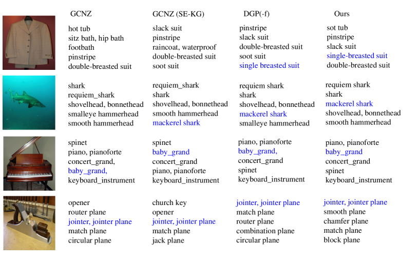
Figure 3: Top-5 prediction for 4 different images from the ImageNet-21k dataset. Predictions ordered by decreasing score, with correct labels are shown in blue.

IV-E Ablation Study

Experiments with Different Variants. In this section, we report experimental results of different variants of residual graph convolutional network on the 2-hops dataset. For fair comparison, we report results on the WordNet knowledge graph, the pretrained ResNet50 is used to extract visual features, and word embeddings are obtained using the GloVe model. Table VI summarizes our experimental results and compares to the GCNZ [15], which adopted plain deep GCN.

TABLE VI: Experimental results for distinct variants on the 2-hops dataset. For fair comparison, all results are reported with ResNet50 and WordNet knowledge graph.

Methods	Hit@k (%)
	1	2	5	10	20
GCNZ [15]	19.80	33.30	53.20	65.40	74.60
Model1	20.28	31.53	47.62	57.42	65.63
Model2	24.03	37.35	56.76	68.65	77.76
Model3	23.91	37.29	56.77	68.63	77.71
Model4	24.21	37.36	56.87	68.86	78.26
Model5	24.20	37.30	56.68	68.58	78.06

TABLE VII: Hit@1 accuracies of the SE-KG with different $k$ and threshold $\alpha$. Testing on the 2-hops dataset.

	0.3	0.5	1.0	5.0
2	26.16	26.68	26.33	26.24
5	26.20	26.26	26.04	25.89
8	26.30	26.48	26.50	26.25
10	26.00	26.20	25.76	25.82

The following obversions can be made from Table VI. First, compared to GCNZ [15], our residual GCN has a significant performance improvement. We can see that our model 4 outperforms the GCNZ by 4.41% on top-1 accuracy. This indicates that the over-smoothing problem is well alleviated and we manage to get performance gains by introducing residual connections. Second, we have not observed advantages for skipping single layer. For the other two connection modes, the hidden layer dimensions have a slight impact on the performance of the model. Third, by increasing the skipping layer of the residual block, the model performance is further improved. Note that adding more GCN layers in the residual block may suffer from over-smoothing problem, three GCN layers are appropriate.

Effectiveness of SE-KG. There are two parameters in our SE-KG, $k$ and $\alpha$. We use grid search to determine the value of parameters. The value of $k$ is search over {2, 5, 8, 10} and $\alpha$ is search over {0.3, 0.5, 1.0, 5.0}. Experimental results are summarized in Table VII. From Table VII, we observe that our model achieves the best results at $k=2$ and $\alpha=0.5$.

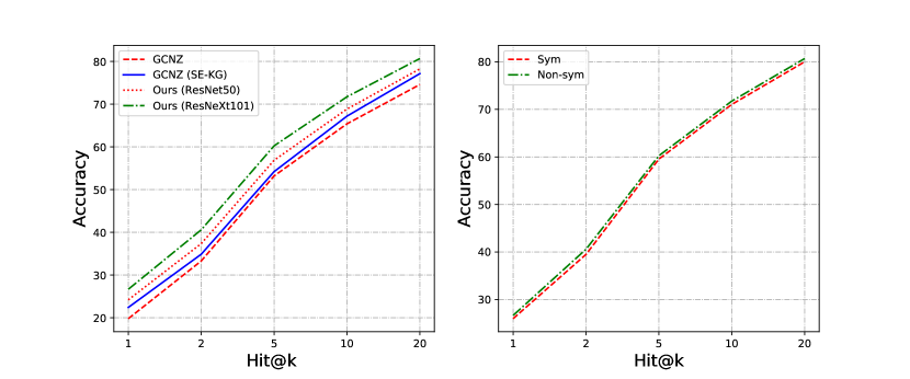
Figure 4: Left: Effectiveness of SE-KG. Right: Effect of the different normalization methods on adjacency matrix. Testing on the 2-hops dataset.

To clear evaluate the performance of SE-KG, we keep the architecture unchanged and retrain GCNZ with our new SE-KG. Experimental results are summarized in Figure. 4. From Figure. 4, we observe that retrained GCNZ (SE-KG) outperform the original model on the all tasks. This indicates that our new SE-KG can further enhance the correlations among categories, and more efficiently propagate information. Since WordNet knowledge graph is built by experts, it is difficult to absorb new categories. Our proposed SE-KG contains both expert knowledge and semantic information, which can easily add new categories to the knowledge graph by connecting new categories to its closer categories. This is a huge advantage of our method.

Symmetric vs. Non-sym Normalization. In this section, we report the experimental result of two normalization methods, Sym, $\hat{\mathcal{A}}=\mathcal{D}^{-\frac{1}{2}}\mathcal{A}\mathcal{D}^{-\frac{1}{2}}$ and Non-sym, $\hat{\mathcal{A}}=\mathcal{D}^{-1}\mathcal{A}$. Experimental results are summarized in Figure. 4. It can be seen from the results that the difference is negligible.

Generalization and Robustness. To comprehensively evaluate the generalization and robustness of our method, we report results with different feature extractors. Concretely, we keep the architecture unchanged and retrained our model with different feature extractors, in this paper, we evaluate our model with the widely-used pre-trained networks including: VGG-19 [53], Inception-V3 [54], DenseNet121 [55], EfficientNet-b0 [56], EfficientNet-b7 [56], ResNet50 [19], ResNeXt101 [57]. During training, we extract the classifier weights from the last layer of a pre-trained CNN as the supervisor. At test time, the backbone network corresponding to the classifier is used to extract visual features. Experimental results are summarized in Table VIII. It can be seen from the results that our model shows better generalization ability and robustness on different architectures.

TABLE VIII: Hit@k performance for the retrained models. Testing on unseen categories.

Test Set	Backbone Network	Hit@k (%)
		1	5	10
2-hops	VGG-19	21.99	52.87	65.28
	ResNet50	24.45	57.20	69.60
	Inception-v3	24.46	57.31	68.82
	DenseNet-121	24.68	58.16	70.23
	EfficientNet-b0	24.70	57.94	69.87
	EfficientNet-b7	25.96	59.88	71.25
	ResNeXt101	26.68	60.25	71.73
3-hops	VGG-19	4.80	15.29	22.26
	ResNet50	5.70	17.71	25.90
	Inception-v3	5.53	17.42	24.91
	DenseNet-121	5.56	17.36	24.96
	EfficientNet-b0	5.59	17.33	24.77
	EfficientNet-b7	5.89	18.31	26.15
	ResNeXt101	6.02	18.35	26.20
All	VGG-19	2.22	7.14	10.65
	ResNet50	2.65	8.30	12.30
	Inception-v3	2.51	8.16	12.00
	DenseNet-121	2.59	8.20	12.04
	EfficientNet-b0	2.55	8.14	11.91
	EfficientNet-b7	2.70	8.68	12.86
	ResNeXt101	2.78	8.76	12.86

V Conclusion

We have developed a novel Residual Graph Convolutional Network for zero-shot learning by introducing the residual connections into the hidden GCN layers. Our model can effectively alleviate the problem of over-smoothing. Moreover, we introduce a new semantic enhanced knowledge graph that contains both expert knowledge and labels semantic information. Our SE-KG can further enhance the correlations among categories and easily absorb new categories into the knowledge graph. Experimental results on two widely used benchmarks have demonstrated the effectiveness of our method. In future work, we would like to investigate the potential of more advanced knowledge graph for ZSL.

References

- [1] Y. Li, J. Zhang, J. Zhang, and K. Huang, “Discriminative learning of latent features for zero-shot recognition,” in Proceedings of the IEEE Conference on Computer Vision and Pattern Recognition, 2018, pp. 7463–7471.
- [2] J. Wei, X. Xu, Y. Yang, Y. Ji, Z. Wang, and H. T. Shen, “Universal weighting metric learning for cross-modal matching,” in Proceedings of the IEEE/CVF conference on computer vision and pattern recognition, 2020, pp. 13 005–13 014.
- [3] J. Wei, Y. Yang, X. Xu, X. Zhu, and H. T. Shen, “Universal weighting metric learning for cross-modal retrieval,” IEEE Transactions on Pattern Analysis and Machine Intelligence, vol. 44, no. 10, pp. 6534–6545, 2022.
- [4] J. Wei, X. Xu, Z. Wang, and G. Wang, “Meta self-paced learning for cross-modal matching,” in Proceedings of the 29th ACM International Conference on Multimedia, 2021, pp. 3835–3843.
- [5] J. Wei, H. Sun, Y. Yang, X. Xu, J. Li, and H. T. Shen, “Semantic guided knowledge graph for large-scale zero-shot learning,” Journal of Visual Communication and Image Representation, vol. 88, p. 103629, 2022.
- [6] R. Socher, M. Ganjoo, C. D. Manning, and A. Ng, “Zero-shot learning through cross-modal transfer,” in Advances in Neural Information Processing Systems, 2013, pp. 935–943.
- [7] A. Frome, G. S. Corrado, J. Shlens, S. Bengio, J. Dean, T. Mikolov et al., “Devise: A deep visual-semantic embedding model,” in Advances in Neural Information Processing Systems, 2013, pp. 2121–2129.
- [8] X. Li, M. Fang, and J. Wu, “Zero-shot classification by transferring knowledge and preserving data structure,” Neurocomputing, vol. 238, pp. 76–83, 2017.
- [9] I. Misra, A. Gupta, and M. Hebert, “From red wine to red tomato: Composition with context,” in Proceedings of the IEEE Conference on Computer Vision and Pattern Recognition, 2017, pp. 1792–1801.
- [10] J. Gao, T. Zhang, and C. Xu, “I know the relationships: Zero-shot action recognition via two-stream graph convolutional networks and knowledge graphs,” in the Association for the Advancement of Artificial Intelligence. AAAI Press, 2019.
- [11] K. Marino, R. Salakhutdinov, and A. Gupta, “The more you know: Using knowledge graphs for image classification,” in IEEE Conference on Computer Vision and Pattern Recognition, 2017, pp. 20–28.
- [12] Z.-M. Chen, X.-S. Wei, P. Wang, and Y. Guo, “Multi-label image recognition with graph convolutional networks,” in Proceedings of the IEEE Conference on Computer Vision and Pattern Recognition, 2019, pp. 5177–5186.
- [13] Y. Fang, K. Kuan, J. Lin, C. Tan, and V. Chandrasekhar, “Object detection meets knowledge graphs,” in Proceedings of the 26th International Joint Conference on Artificial Intelligence, 2017, pp. 1661–1667.
- [14] T. N. Kipf and M. Welling, “Semi-supervised classification with graph convolutional networks,” in International Conference for Learning Representation, 2017.
- [15] X. Wang, Y. Ye, and A. Gupta, “Zero-shot recognition via semantic embeddings and knowledge graphs,” in Proceedings of the IEEE Conference on Computer Vision and Pattern Recognition, 2018, pp. 6857–6866.
- [16] G. A. Miller, “Wordnet: a lexical database for english,” Communications of the ACM, vol. 38, no. 11, pp. 39–41, 1995.
- [17] Q. Li, Z. Han, and X.-M. Wu, “Deeper insights into graph convolutional networks for semi-supervised learning,” in Thirty-Second AAAI Conference on Artificial Intelligence, 2018.
- [18] A. Veit, M. J. Wilber, and S. Belongie, “Residual networks behave like ensembles of relatively shallow networks,” in Advances in neural information processing systems, 2016, pp. 550–558.
- [19] K. He, X. Zhang, S. Ren, and J. Sun, “Deep residual learning for image recognition,” in Proceedings of the IEEE Conference on Computer Vision and Pattern Recognition, 2016, pp. 770–778.
- [20] C. H. Lampert, H. Nickisch, and S. Harmeling, “Attribute-based classification for zero-shot visual object categorization,” IEEE Transactions on Pattern Analysis and Machine Intelligence, vol. 36, no. 3, pp. 453–465, 2014.
- [21] Z. Ji, Y. Xie, Y. Pang, L. Chen, and Z. Zhang, “Zero-shot learning with multi-battery factor analysis,” Signal Processing, vol. 138, pp. 265–272, 2017.
- [22] S. Changpinyo, W.-L. Chao, and F. Sha, “Predicting visual exemplars of unseen classes for zero-shot learning,” in Proceedings of the IEEE International Conference on Computer Vision, 2017, pp. 3476–3485.
- [23] M. Norouzi, T. Mikolov, S. Bengio, Y. Singer, J. Shlens, A. Frome, G. Corrado, and J. Dean, “Zero-shot learning by convex combination of semantic embeddings,” in International Conference for Learning Representation, 2014.
- [24] S. Changpinyo, W.-L. Chao, B. Gong, and F. Sha, “Synthesized classifiers for zero-shot learning,” in Proceedings of the IEEE Conference on Computer Vision and Pattern Recognition, 2016, pp. 5327–5336.
- [25] C.-W. Lee, W. Fang, C.-K. Yeh, and Y.-C. Frank Wang, “Multi-label zero-shot learning with structured knowledge graphs,” in Proceedings of the IEEE Conference on Computer Vision and Pattern Recognition, 2018, pp. 1576–1585.
- [26] J. Pennington, R. Socher, and C. Manning, “Glove: Global vectors for word representation,” in Proceedings of the 2014 Conference on Empirical Methods in Natural Language Processing, 2014, pp. 1532–1543.
- [27] X. Bing, N. Wang, T. Chen, and L. Mu, “Empirical evaluation of rectified activations in convolutional network,” Computer Science, 2015.
- [28] D. Kingma and J. Ba, “Adam: A method for stochastic optimization,” in European Conference on Computer Vision, 2014.
- [29] D. Mandal, S. Narayan, S. K. Dwivedi, V. Gupta, S. Ahmed, F. S. Khan, and L. Shao, “Out-of-distribution detection for generalized zero-shot action recognition,” in Proceedings of the IEEE Conference on Computer Vision and Pattern Recognition, 2019, pp. 9985–9993.
- [30] J. Deng, W. Dong, R. Socher, L.-J. Li, K. Li, and L. Fei-Fei, “Imagenet: A large-scale hierarchical image database,” in 2009 IEEE Conference on Computer Vision and Pattern Recognition. IEEE, 2009, pp. 248–255.
- [31] Y. Fu, T. M. Hospedales, T. Xiang, and S. Gong, “Transductive multi-view zero-shot learning,” IEEE Transactions on Pattern Analysis and Machine Intelligence, vol. 37, no. 11, pp. 2332–2345, 2015.
- [32] C. H. Lampert, H. Nickisch, and S. Harmeling, “Learning to detect unseen object classes by between-class attribute transfer,” in 2009 IEEE Conference on Computer Vision and Pattern Recognition. IEEE, 2009, pp. 951–958.
- [33] Z. Akata, F. Perronnin, Z. Harchaoui, and C. Schmid, “Label-embedding for attribute-based classification,” in Proceedings of the IEEE Conference on Computer Vision and Pattern Recognition, 2013, pp. 819–826.
- [34] A. L. Maas, A. Y. Hannun, and A. Y. Ng, “Rectifier nonlinearities improve neural network acoustic models,” in International Conference on Machine Learning. Citeseer, 2013.
- [35] O. Russakovsky, J. Deng, H. Su, J. Krause, S. Satheesh, S. Ma, Z. Huang, A. Karpathy, A. Khosla, M. Bernstein et al., “Imagenet large scale visual recognition challenge,” International Journal of Computer Vision, vol. 115, no. 3, pp. 211–252, 2015.
- [36] Z. Akata, S. Reed, D. Walter, H. Lee, and B. Schiele, “Evaluation of output embeddings for fine-grained image classification,” in Proceedings of the IEEE Conference on Computer Vision and Pattern Recognition, 2015, pp. 2927–2936.
- [37] Y. Long, L. Liu, L. Shao, F. Shen, G. Ding, and J. Han, “From zero-shot learning to conventional supervised classification: Unseen visual data synthesis,” in Proceedings of the IEEE Conference on Computer Vision and Pattern Recognition, 2017, pp. 1627–1636.
- [38] H. Nakayama and N. Nishida, “Zero-resource machine translation by multimodal encoder–decoder network with multimedia pivot,” Machine Translation, vol. 31, no. 1-2, pp. 49–64, 2017.
- [39] N. Nakashole and R. Flauger, “Knowledge distillation for bilingual dictionary induction,” in Proceedings of the 2017 Conference on Empirical Methods in Natural Language Processing, 2017, pp. 2497–2506.
- [40] Y. Ma, E. Cambria, and S. Gao, “Label embedding for zero-shot fine-grained named entity typing,” in Proceedings of COLING 2016, the 26th International Conference on Computational Linguistics: Technical Papers, 2016, pp. 171–180.
- [41] M. Palatucci, D. Pomerleau, G. E. Hinton, and T. M. Mitchell, “Zero-shot learning with semantic output codes,” in International Conference on Neural Information Processing Systems, 2009.
- [42] N. Srivastava, G. Hinton, A. Krizhevsky, I. Sutskever, and R. Salakhutdinov, “Dropout: a simple way to prevent neural networks from overfitting,” The Journal of Machine Learning Research, vol. 15, no. 1, pp. 1929–1958, 2014.
- [43] W. Wang, V. W. Zheng, H. Yu, and C. Miao, “A survey of zero-shot learning: Settings, methods, and applications,” ACM Transactions on Intelligent Systems and Technology (TIST), vol. 10, no. 2, p. 13, 2019.
- [44] X. Li, S. Liao, W. Lan, X. Du, and G. Yang, “Zero-shot image tagging by hierarchical semantic embedding,” in Proceedings of the 38th International ACM SIGIR Conference on Research and Development in Information Retrieval. ACM, 2015, pp. 879–882.
- [45] L. Gao, J. Song, J. Shao, X. Zhu, and H. Shen, “Zero-shot image categorization by image correlation exploration,” in Proceedings of the 5th ACM on International Conference on Multimedia Retrieval. ACM, 2015, pp. 487–490.
- [46] H. Li, D. Li, and X. Luo, “Bap: Bimodal attribute prediction for zero-shot image categorization,” in Proceedings of the 22nd ACM international conference on Multimedia. ACM, 2014, pp. 1013–1016.
- [47] Y. Long and L. Shao, “Learning to recognise unseen classes by a few similes,” in Proceedings of the 25th ACM international conference on Multimedia. ACM, 2017, pp. 636–644.
- [48] G. Yang, J. Liu, J. Xu, and X. Li, “Dissimilarity representation learning for generalized zero-shot recognition,” in 2018 ACM Multimedia Conference on Multimedia Conference. ACM, 2018, pp. 2032–2039.
- [49] Y. Xian, C. H. Lampert, B. Schiele, and Z. Akata, “Zero-shot learning-a comprehensive evaluation of the good, the bad and the ugly,” IEEE transactions on pattern analysis and machine intelligence, 2018.
- [50] V. Kumar Verma, G. Arora, A. Mishra, and P. Rai, “Generalized zero-shot learning via synthesized examples,” in Proceedings of the IEEE conference on computer vision and pattern recognition, 2018, pp. 4281–4289.
- [51] H. Zhang and P. Koniusz, “Zero-shot kernel learning,” in Proceedings of the IEEE Conference on Computer Vision and Pattern Recognition, 2018, pp. 7670–7679.
- [52] M. Kampffmeyer, Y. Chen, X. Liang, H. Wang, Y. Zhang, and E. P. Xing, “Rethinking knowledge graph propagation for zero-shot learning,” in Proceedings of the IEEE Conference on Computer Vision and Pattern Recognition, 2019, pp. 11 487–11 496.
- [53] K. Simonyan and A. Zisserman, “Very deep convolutional networks for large-scale image recognition,” in Proceedings of the International Conference on Learning Representations, 2015.
- [54] C. Szegedy, V. Vanhoucke, S. Ioffe, J. Shlens, and Z. Wojna, “Rethinking the inception architecture for computer vision,” in Proceedings of the IEEE conference on computer vision and pattern recognition, 2016, pp. 2818–2826.
- [55] G. Huang, Z. Liu, L. Van Der Maaten, and K. Q. Weinberger, “Densely connected convolutional networks,” in Proceedings of the IEEE conference on computer vision and pattern recognition, 2017, pp. 4700–4708.
- [56] M. Tan and Q. Le, “Efficientnet: Rethinking model scaling for convolutional neural networks,” in International Conference on Machine Learning, 2019, pp. 6105–6114.
- [57] S. Xie, R. Girshick, P. Dollár, Z. Tu, and K. He, “Aggregated residual transformations for deep neural networks,” in Proceedings of the IEEE conference on computer vision and pattern recognition, 2017, pp. 1492–1500.
- [58] J. Wei, Y. Yang, J. Li, L. Zhu, L. Zuo, and H. T. Shen, “Residual graph convolutional networks for zero-shot learning,” in Proceedings of the ACM Multimedia Asia on ZZZ, 2019, pp. 1–6.
- [59] X. Xu, H. Lu, J. Song, Y. Yang, H. T. Shen, and X. Li, “Ternary adversarial networks with self-supervision for zero-shot cross-modal retrieval,” IEEE transactions on cybernetics, 2019.
- [60] F. Shen, X. Zhou, J. Yu, Y. Yang, L. Liu, and H. T. Shen, “Scalable zero-shot learning via binary visual-semantic embeddings,” IEEE Transactions on Image Processing, vol. 28, no. 7, pp. 3662–3674, 2019.
- [61] J. Li, M. Jing, K. Lu, L. Zhu, Y. Yang, and Z. Huang, “Alleviating feature confusion for generative zero-shot learning,” in Proceedings of the 27th ACM International Conference on Multimedia, 2019, pp. 1587–1595.
- [62] Y. Xu, Y. Yang, F. Shen, X. Xu, Y. Zhou, and H. T. Shen, “Attribute hashing for zero-shot image retrieval,” in 2017 IEEE International Conference on Multimedia and Expo (ICME). IEEE, 2017, pp. 133–138.
- [63] Y. Yang, Y. Luo, W. Chen, F. Shen, J. Shao, and H. T. Shen, “Zero-shot hashing via transferring supervised knowledge,” in Proceedings of the 24th ACM international conference on Multimedia, 2016, pp. 1286–1295.
- [64] J. Li, M. Jing, K. Lu, Z. Ding, L. Zhu, and Z. Huang, “Leveraging the invariant side of generative zero-shot learning,” in Proceedings of the IEEE Conference on Computer Vision and Pattern Recognition, 2019, pp. 7402–7411.
- [65] X. Xu, F. Shen, Y. Yang, D. Zhang, H. Tao Shen, and J. Song, “Matrix tri-factorization with manifold regularizations for zero-shot learning,” in Proceedings of the IEEE conference on computer vision and pattern recognition, 2017, pp. 3798–3807.
- [66] Y. L. Cacheux, H. L. Borgne, and M. Crucianu, “Modeling inter and intra-class relations in the triplet loss for zero-shot learning,” in Proceedings of the IEEE International Conference on Computer Vision, 2019, pp. 10 333–10 342.
- [67] Y. Xian, T. Lorenz, B. Schiele, and Z. Akata, “Feature generating networks for zero-shot learning,” in Proceedings of the IEEE conference on computer vision and pattern recognition, 2018, pp. 5542–5551.
- [68] V. K. Verma and P. Rai, “A simple exponential family framework for zero-shot learning,” in Joint European Conference on Machine Learning and Knowledge Discovery in Databases. Springer, 2017, pp. 792–808.
- [69] Y. Zhu, J. Xie, B. Liu, and A. Elgammal, “Learning feature-to-feature translator by alternating back-propagation for generative zero-shot learning,” in Proceedings of the IEEE International Conference on Computer Vision, 2019, pp. 9844–9854.
- [70] B. Romera-Paredes and P. Torr, “An embarrassingly simple approach to zero-shot learning,” in International Conference on Machine Learning, 2015, pp. 2152–2161.
- [71] A. Paszke, S. Gross, S. Chintala, G. Chanan, E. Yang, Z. DeVito, Z. Lin, A. Desmaison, L. Antiga, and A. Lerer, “Automatic differentiation in pytorch,” in Conference on Neural Information Processing Systems Workshop, 2017.
- [72] Y. Ji, Y. Zhan, Y. Yang, X. Xu, F. Shen, and H. T. Shen, “A knowledge map guided coarse-to-fine action recognition,” IEEE Trans. Image Processing, 2019.
- [73] X. Zhou, F. Shen, L. Liu, W. Liu, L. Nie, Y. Yang, and H. T. Shen, “Graph convolutional network hashing,” IEEE transactions on cybernetics, 2018.
- [74] B. Wang, Y. Yang, X. Xu, A. Hanjalic, and H. T. Shen, “Adversarial cross-modal retrieval,” in Proceedings of the 2017 ACM on Multimedia Conference, 2017, pp. 154–162.
- [75] X. Xu, F. Shen, Y. Yang, H. T. Shen, and X. Li, “Learning discriminative binary codes for large-scale cross-modal retrieval,” IEEE Trans. Image Processing, vol. 26, no. 5, pp. 2494–2507, 2017.
- [76] S. Rahman, S. Khan, and F. Porikli, “A unified approach for conventional zero-shot, generalized zero-shot, and few-shot learning,” IEEE Transactions on Image Processing, vol. 27, no. 11, pp. 5652–5667, 2018.
- [77] Y. Annadani and S. Biswas, “Preserving semantic relations for zero-shot learning,” in Proceedings of the IEEE Conference on Computer Vision and Pattern Recognition, 2018, pp. 7603–7612.
- [78] C. Zhang, X. Lyu, and Z. Tang, “Tgg: Transferable graph generation for zero-shot and few-shot learning,” in Proceedings of the 27th ACM International Conference on Multimedia, 2019, pp. 1641–1649.
- [79] T. Hascoet, Y. Ariki, and T. Takiguchi, “On zero-shot recognition of generic objects,” in Proceedings of the IEEE Conference on Computer Vision and Pattern Recognition, 2019, pp. 9553–9561.
- [80] S. Liu, J. Chen, L. Pan, C.-W. Ngo, T.-S. Chua, and Y.-G. Jiang, “Hyperbolic visual embedding learning for zero-shot recognition,” in Proceedings of the IEEE/CVF Conference on Computer Vision and Pattern Recognition, 2020, pp. 9273–9281.
- [81] Y. Yu, Z. Ji, X. Li, J. Guo, Z. Zhang, H. Ling, and F. Wu, “Transductive zero-shot learning with a self-training dictionary approach,” IEEE transactions on cybernetics, vol. 48, no. 10, pp. 2908–2919, 2018.
- [82] Y. Yu, Z. Ji, J. Guo, and Z. Zhang, “Zero-shot learning via latent space encoding,” IEEE transactions on cybernetics, vol. 49, no. 10, pp. 3755–3766, 2018.
- [83] X. Xu, I. W. Tsang, and C. Liu, “Complementary attributes: A new clue to zero-shot learning,” IEEE transactions on cybernetics, 2019.