Orthogonal Series Estimation for the Ratio of Conditional Expectation Functions

Abstract

In various fields of data science, researchers are often interested in estimating the ratio of conditional expectation functions (CEFR). Specifically in causal inference problems, it is sometimes natural to consider ratio-based treatment effects, such as odds ratios and hazard ratios, and even difference-based treatment effects are identified as CEFR in some empirically relevant settings. This chapter develops the general framework for estimation and inference on CEFR, which allows the use of flexible machine learning for infinite-dimensional nuisance parameters. In the first stage of the framework, the orthogonal signals are constructed using debiased machine learning techniques to mitigate the negative impacts of the regularization bias in the nuisance estimates on the target estimates. The signals are then combined with a novel series estimator tailored for CEFR. We derive the pointwise and uniform asymptotic results for estimation and inference on CEFR, including the validity of the Gaussian bootstrap, and provide low-level sufficient conditions to apply the proposed framework to some specific examples. We demonstrate the finite-sample performance of the series estimator constructed under the proposed framework by numerical simulations. Finally, we apply the proposed method to estimate the causal effect of the 401(k) program on household assets.

1 Introduction

In various fields of data science, researchers often face problems of estimating the ratio of conditional expectation functions (CEFR). Although CEFR appears not only in causal inference studies, there are several important examples of CEFR in the treatment effect estimation literature. When an outcome of interest is the relapse rate of a specific disease, it is more natural to consider the ratio of the conditional expectation of potential outcomes $E[Y_{1}|X]/E[Y_{0}|X]$, rather than the difference $E[Y_{1}|X]-E[Y_{0}|X]$, as a measure of causal effects of a medical treatment, where $Y_{1}$ and $Y_{0}$ are the potential outcome with and without a treatment, respectively, and $X$ is a vector of baseline covariates. Likewise, ratio-based treatment effects such as the odds ratio and hazard ratio have been widely used especially in clinical settings. Furthermore, in a data combination setting where an outcome and a treatment status are only separately observed, both conditional average treatment effect (CATE) and local average treatment effect (LATE) are identified as in the form of CEFR (Yamane et al., 2018; Shinoda and Hoshino, 2022), while these effects are defined as the difference of the potential outcomes.

In this article, we start by developing a novel series estimator for CEFR in a very simple setting without selection bias in observed data. This series estimator is itself useful in estimating treatment effects when data can be collected completely at random from the population of interest, but such randomized data are often not available in practice. Technically, when there is selection bias in collected data, we need to estimate potentially infinite-dimensional nuisance parameters to adjust for the bias, but these parameters may be hard to estimate with a “sufficiently high quality” in observational studies on complex systems since they can be very high-dimensional and/or highly nonlinear. The highly complex nuisance parameters do not satisfy the traditional assumptions that limit the complexity of a function class, and therefore the resulting semiparametric estimator fails to be $\sqrt{N}$-consistent. We employ debiased machine learning (DML), a set of techniques to enable the use of flexible machine learning (ML) methods for nuisance estimation, to develop a simple and general framework for constructing a high-quality estimator for CEFR even in the presence of selection bias in observed data.

The major contribution of this study is the development of a novel inference framework for CEFR with theoretical guarantees. We derive the general asymptotic results for estimation and uniform inference on the best linear approximation to the target CEFR under the proposed framework, including the validity of the Gaussian bootstrap. It is worth noting that we do not have to add stronger regularity conditions than the assumptions previously known in the literature to establish the theoretical results in this article. In addition to the general results, we provide a set of low-level sufficient conditions to apply the proposed framework to several specific settings. Besides the asymptotic analysis, we conduct numerical simulations to evaluate the performance of the proposed method on finite samples. We also illustrate the use of the framework in an empirical example.

This study builds upon three important bodies of research within the semiparametric literature: DML, series estimation and CEFR estimation. DML (Chernozhukov et al., 2018, 2022a) enables inference on the finite-dimensional parameter in the presence of infinite-dimensional nuisance parameters by using the Neyman orthogonal moment conditions. When the moment condition satisfies the Neyman orthogonality (Neyman, 1959), bias in the nuisance estimates has no first-order asymptotic effect on the estimator of the target parameter. DML is powerful enough to allow the use of a broad class of ML estimators —such as $\ell_{1}$-penalized methods in sparse models (Bickel et al., 2009; Bühlmann and van de Geer, 2011; Belloni et al., 2011, 2012; Belloni and Chernozhukov, 2011, 2013), $L_{2}$-boosting methods in sparse linear models (Luo et al., 2016), neural nets (Schmidt-Hieber, 2020; Farrell et al., 2021; Kohler and Langer, 2021), trees and random forest (Wager and Walther, 2015; Syrgkanis and Zampetakis, 2020)— under a broad range of data generating processes and for various causal parameters. Moreover, the extensions of DML have been proposed to estimate a function, e.g. CATE or continuous treatment effect, with the existence of complex infinite-dimensional nuisance parameters (Jacob, 2019; Zimmert and Lechner, 2019; Colangelo and Lee, 2020; Semenova and Chernozhukov, 2021; Fan et al., 2022). The present study provides a novel method for the orthogonal estimation under a variety of realistic settings that cannot be covered by the previous works, such as ratio-based treatment effects, and treatment effects in the data combination settings.

The second foundation of this study is the least squares series estimation. Series estimation is a type of nonparametric estimation method that approximates a function of interest by a linear combination of multiple basis functions. It is especially useful when the exact functional form of the target function is unknown. Its asymptotic properties have been investigated intensively in the literature (van de Geer, 1990; Andrews, 1991; Eastwood and Gallant, 1991; Gallant and Souza, 1991; Newey, 1997; van de Geer, 2002; Huang, 2003; Chen, 2007; Cattaneo and Farrell, 2013; Belloni et al., 2015; Chen and Christensen, 2015), among which we will mainly rely on the results in Belloni et al. (2015). This study contributes to the series estimation literature by establishing the asymptotic theory for the CEFR problems rather than the standard regression setting.

This study is also closely related to CEFR estimation in causal inference. A simple yet important example is ratio-based treatment effects such as the odds and hazard ratio. To the best of our knowledge, the previous works on the estimation of the ratio-based treatment effects all impose assumptions on the functional form somewhere in the model (Dukes and Vansteelandt, 2018; Liang and Yu, 2020; Yadlowsky et al., 2021; Lee, 2022). For example, Liang and Yu (2020) supposes that the ratio-based treatment effects can be expressed as the monotone single index model, and Yadlowsky et al. (2021) imposes a stronger condition that the monotone link function is an exponential function. On the other hand, this study considers a fully nonparametric model for treatment effects, imposing no assumptions on the functional form of CEFR.

Furthermore, Yamane et al. (2018) and Shinoda and Hoshino (2022) show that difference-based CATE and LATE are identified in the form of CEFR in the data combination setting where we cannot observe an outcome and a treatment status simultaneously in a single dataset, and develop estimation methods for CEFR. This study accommodates the generalized version of their problem settings, where each separate dataset contains selection bias. Their estimators cannot handle the selection bias without introducing additional nuisance parameters, but their methods are not orthogonal to the nuisance parameters.

The rest of this article is organized as follows. In Section 2, we develop a simple series estimator for CEFR. We propose the general framework for estimation and inference of CEFR in Section 3. The main theoretical results for the asymptotic properties of the series estimator under the proposed framework are presented in Section 4, and the application of the framework to some specific treatment effects problems is shown in Section 5. In Section 6, we illustrate the finite sample performance of the proposed method by numerical simulations. We also apply the proposed method to the empirical example of estimating a causal effect of participation in 401(k) on net financial assets in Section 7. Finally, we provide further discussion on the limitation and future direction of the present study in Section 8.

2 Direct Series Estimator for CEFR

Consider the following model:

$$\theta_{0}(X)=\frac{\nu_{0}(X)}{\zeta_{0}(X)},\hskip 14.22636ptU=\nu_{0}(X)+\varepsilon_{U},\hskip 14.22636ptT=\zeta_{0}(X)+\varepsilon_{T},$$

$$E[\varepsilon_{U}|X]=E[\varepsilon_{T}|X]=0,$$ (1)

where $X\in\mathcal{X}\subset\mathbb{R}^{q}$ is a $q$-dimensional vector of covariates, and $\zeta_{0}(x)\neq 0$ for all $x\in\mathcal{X}$ is necessary for $\theta_{0}(x)$ to be well-defined. Now we are interested in estimating $\theta_{0}(x)$ from separately observed iid samples: $\{u_{i},x_{i}\}_{i=1}^{N_{U}}$ of $(U,X)$ and $\{t_{i},x_{i}\}_{i=1}^{N_{T}}$ of $(T,X)$. Suppose $N=N_{U}=N_{T}$ without loss of generality. Also, assume that the samples $\{u_{i},x_{i}\}_{i=1}^{N}$ and $\{t_{i},x_{i}\}_{i=1}^{N}$ are complete random draws from the population of interest, i.e. there is no selection bias in these separate samples. Then, regarding $U$ and $T$ as outcome variables with and without a treatment, respectively, this problem coincides with the estimation of ratio-based treatment effects (Ogburn et al., 2015; Dukes and Vansteelandt, 2018; Yadlowsky et al., 2021) in randomized control trials. Moreover, estimation of difference-based CATE and LATE from separately observed samples (Yamane et al., 2018; Shinoda and Hoshino, 2022) is included in the model (1). Although the estimator developed below primarily aims at estimating $\theta_{0}(x)$ from the separate samples, it can also be applicable to the estimation from joint samples $\{u_{i},t_{i},x_{i}\}_{i=1}^{N}$ of $(U,T,X)$. Thereafter, we omit arguments of functions if they are obvious from the context.

It follows from the model (1) that $E[U-\zeta_{0}(X)\theta_{0}(X)|X]=0$. Then, using this moment condition, we can consider the linear approximation to the target function $\theta_{0}(x)$ by a vector of $k$ basis functions $p(x):=(p_{1}(x),\ldots,p_{k}(x))^{\prime}$ as $\theta(x)=p(x)^{\prime}\beta$, where

$$\beta =\underset{b\in\mathbb{R}^{k}}{\mathrm{argmin}}E[(U-\zeta_{0}(X)p(X)^{\prime}b)^{2}]$$

$$=E[p(X)p(X)^{\prime}\zeta_{0}(X)^{2}]^{-1}E[p(X)\zeta_{0}(X)U].$$ (2)

However, as the true denominator function $\zeta_{0}(x)$ is unknown, the above equation cannot be directly applied for estimation. To deal with this issue, Shinoda and Hoshino (2022) proposed to plug-in the estimator $\hat{\zeta}(x)$ of $\zeta_{0}(x)$, while Yamane et al. (2018) introduced an auxiliary function and reformulate the problem into minimax optimization. Both of these approaches have problems: the former lacks the theoretical justification to use flexible nonparametric methods for $\hat{\zeta}(x)$ since simply plugging-in nonparametric estimates generally does not ensure $\sqrt{N}$-consistency of the target estimator, and the latter suffers from unreliable hyperparameter selection caused by the minimax objective. In what follows, we develop a simpler one-step estimator for CEFR in the spirit of Vapnik (1999)’s principle: When solving a given problem, try to avoid solving a more general problem as an intermediate step.

Define $f(x):=\zeta_{0}(x)p(x)$ and its series estimator

$$\hat{f}(x):=E[p(X)p(X)^{\prime}T]E[p(X)p(X)^{\prime}]^{-1}p(x)=:QS^{-1}p(x).$$

Substituting $f$ for (2) gives

$$\beta=E[f(X)f(X)^{\prime}]^{-1}E[f(X)U].$$

Then, by replacing $f(x)$ with its estimator $\hat{f}(x)$, we obtain

$$\beta =(QS^{-1}SS^{-1}Q)^{-1}QS^{-1}E[p(X)U]$$

$$=Q^{-1}SQ^{-1}QS^{-1}E[p(X)U]$$

$$=Q^{-1}E[p(X)U],$$

and its sample analog estimator $\hat{\beta}=\hat{Q}^{-1}E_{N}[p(x_{i})u_{i}]$, where $E_{N}[g(x_{i})]:=N^{-1}\sum_{i=1}^{N}f(x_{i})$ for some function $g$ and $\hat{Q}:=E_{N}[p(x_{i})p(x_{i})^{\prime}t_{i}]$. The key observation here is that we can compute $\hat{\beta}$ even when $\{u_{i},x_{i}\}_{i=1}^{N}$ and $\{t_{i},x_{i}\}_{i=1}^{N}$ are only separately observed. Henceforth, we refer to this estimator as the Direct Series Ratio (DSR) estimator.

Remark 2.1 (Asymptotic Properties of the DSR Estimator).

Although the estimator $\hat{f}(x)$ is plugged-in during the derivation process of DSR, there is no actual need to calculate $\hat{f}(x)$. Using the nonparametric estimator of nuisance functions as done in Shinoda and Hoshino (2022) may adversely affect the theoretical and practical properties of a target estimator since nonparametric estimators may have biases due to model selection and regularization. DSR, on the other hand, does not require the estimated value. Consequently, it converges at the same rate as in the general regression setting under mild conditions. The pointwise and uniform asymptotic theory for the DSR estimator immediately follows from the theoretical results shown in 4.

Remark 2.2 (Regularized Estimation).

For practical purposes, the estimation of $\hat{Q}$ can be unstable when the sample size is small or when $\hat{Q}$ is close to a singular matrix. One way to stabilize the estimation is to perform $\ell_{2}$-regularization (ridge estimation) with $\lambda$ as the regularization parameter:

$$\tilde{\beta}=(\hat{Q}+\lambda I_{k})^{-1}E_{N}[p(x_{i})u_{i}].$$ (3)

The impact of $\lambda$ on the performance of DSR is investigated in the simulation study in Section 6.1.

Remark 2.3 (Model Selection).

To implement the estimators $\hat{\beta}$ and $\tilde{\beta}$, we need to choose the series length $k$ and the regularization parameter $\lambda$. One practical way of selection is to find hyperparameters that minimize a criterion computed based on cross-validation (CV). The Mean Squared Error (MSE) is a general criterion, but it is difficult to evaluate MSE directly in the setting (1). However, in special cases where $\zeta_{0}(x)>0$ for all $x\in\mathcal{X}$, it is possible to calculate a CV criterion that preserves the rank order of MSE. Expanding MSE gives

$$E[(U-\zeta_{0}(X)\hat{\theta}(X))^{2}]=E[U^{2}]-2E[U\zeta_{0}(X)\hat{\theta}(X)]+E[\zeta_{0}(X)^{2}\hat{\theta}(X)^{2}],$$

and we can ignore the first term as it does not involve the estimator $\hat{\theta}$. Moreover, if $\zeta_{0}(x)$ is positive for all $x\in\mathcal{X}$,

$$E[\zeta_{0}(X)\hat{\theta}(X)^{2}]-2E[U\hat{\theta}(X)]$$

is monotone increasing in MSE. Therefore, we can use the sample analogue as the criterion:

$$E_{N}[t_{i}\hat{\theta}(x_{i})^{2}]-2E_{N}[u_{i}\hat{\theta}(x_{i})].$$ (4)

CV in the general situation where $\zeta_{0}$ can take negative values is a subject for future work. This limitation, however, does not detract significantly from the value of this study since researchers often have a priori knowledge that $\zeta_{0}(x)$ is positive in many practical situations. Some of these situations are explained in Section 5.

3 General Framework for Estimation and Inference of CEFR

In this section, we propose a general framework for the CEFR problems by using DSR developed in the previous section as one of the building blocks. The proposed framework is based on the generalized version of the model (1), and therefore it can accommodate a variety of real-world applications.

3.1 Setup

In observational studies of complex systems, possibly high-dimensional covariates $X$ may be necessary for conditional independence to hold, which is one of the critical conditions in many causal inference problems. However, researchers are often not interested in estimating treatment effects as a function of all covariates, but they need to focus on the heterogeneous relationships between treatment effects and only a few important factors. In such a case, estimating the target function on the full vector $X$ is unnecessarily hard due to the curse of dimensionality, and directly estimating a function of a subvector can stabilize the estimation. Therefore, suppose that our parameter of interest $\theta_{0}$ is now a function of $V\in\mathcal{V}$, a subvector of covariates $X$. Also, suppose that $\nu_{0}$ and $\zeta_{0}$ in (1) are defined as

$$\nu_{0}(v)=E[U(O,\eta_{0})|V=v],\hskip 14.22636pt\zeta_{0}(v)=E[T(O,\eta_{0})|V=v],$$ (5)

where the random variables $U$ and $T$ depend on a vector of observed random variables $O$ and a set of infinite-dimensional nuisance parameters $\eta_{0}(x)$. Note that $\eta_{0}$ is a function of $X$, reflecting that $X$ is indispensable for adjusting for selection biases. We refer to $U$ and $T$ as signals, following Semenova and Chernozhukov (2021), and use the notations $U_{0}:=U(O,\eta_{0})$ and $T_{0}:=T(O,\eta_{0})$.

Among many possible choices of the signals $U$ and $T$ that satisfy (5), we focus on the signals with the Neyman orthogonal property, which is defined later. The Neyman orthogonality is the key property to deliver high-quality inference on the target function $\theta_{0}(v)$ even when modern ML estimators that do not satisfy Donsker conditions are used for the nuisance functions $\eta_{0}$. The classic semiparametric theories ensure that the target estimator achieves $\sqrt{N}$-consistency by bounding the complexity of the nuisance space, but estimators in such a restricted class are not suitable for fitting high-dimensional and/or highly nonlinear nuisance functions in data-rich environments. On the other hand, modern ML estimators are so flexible to fit any function that there is no need to specify the functional form of the nuisance parameters in advance. ML estimators also perform well in high-dimensional settings by employing regularization to reduce variance at the cost of regularization bias. These properties are especially important in observational studies in which the distribution of an outcome is a complex mixture of treated and non-treated populations, and there are many confounding factors.

Although ML estimators are effective in predicting the values of nuisance functions, their prediction is inherently biased by model selection and regularization. Therefore, the naive plug-in estimator of the target function fails to be $\sqrt{N}$-consistent. To ensure the desirable theoretical properties of the target estimator while using flexible ML estimators for nuisance functions, we need signals that are locally insensitive to the bias of the nuisance estimators. Formally, the Neyman orthogonality is defined in terms of the pathwise (Gateaux) derivative as follows:

$$\partial_{s}E[U(O,\eta_{0}+s(\eta-\eta_{0}))-\nu_{0}(V)|V=v]|_{s=0} =0,$$

$$\partial_{s}E[T(O,\eta_{0}+s(\eta-\eta_{0}))-\zeta_{0}(V)|V=v]|_{s=0} =0,$$

for all $v\in\mathcal{V}$, where $\partial$ is the partial derivative operator and $s\in[0,1]$ is a constant.

3.2 Examples

We describe some empirically relevant examples for the generalized setting. The detailed discussions on conditions for identification and inference of estimands in each example are given in Section 5.

Example 3.1 (Local Average Treatment Effect).

Let $Y_{1}$ and $Y_{0}$ be the potential outcomes realized only when an individual is treated and not treated, respectively. Similarly, let $D_{1}$ and $D_{0}$ be the potential treatment status realized only when an individual is assigned to a treatment group or not. We also denote a binary treatment assignment as $Z$. The observable is $O=(Y,D,Z,X)$, where $D=ZD_{1}+(1-Z)D_{0}$ is a realized treatment status, and $Y=DY_{1}+(1-D)Y_{0}$ is a realized outcome. The parameter of interest is LATE, which is defined as a treatment effect measured for the subpopulation of compliers

$$\theta_{0}(v)=E[Y_{1}-Y_{0}|D_{1}>D_{0},V=v],$$

where compliers are individuals who always follow the given assignment $Z$. LATE is often used when there is self-selection to receive a treatment (often referred to as noncompliance to treatment assignment), and thus the observed covariates $X$ are insufficient to adjust for selection bias in $D$.

A standard identification strategy for LATE is using $Z$ as an instrument to $D$. Under several assumptions including conditions necessary for $Z$ to be a valid instrument, LATE is identified as

$$\theta_{0}(v)=\frac{E[E[Y|Z=1,X]-E[Y|Z=0,X]|V=v]}{E[E[D|Z=1,X]-E[D|Z=0,X]|V=v]}.$$

Therefore, we can consider LATE estimation as a problem of CEFR by setting $\nu_{0}(v)=E[\mu_{0}(1,X)-\mu_{0}(0,X)|V=v]$ and $\zeta_{0}(v)=E[\pi_{0}(1,X)-\pi_{0}(0,X)|V=v]$, where $\mu_{0}(z,x)=E[Y|Z=z,X=x]$ and $\pi_{0}(z,x)=E[D|Z=z,X=x]$.

Example 3.2 (Ratio-Based Treatment Effects).

The observable vector is $O=(Y,D,X)$, where $Y$ is an outcome of interest, and $D$ is a binary treatment status. As in the case of LATE, let $Y_{1}$ and $Y_{0}$ be the potential outcomes. The parameter of interest is the ratio-based CATE:

$$\theta_{0}(v)=\frac{E[Y_{1}|V=v]}{E[Y_{0}|V=v]},$$

where $E[Y_{0}|V=v]\neq 0$ for all $v\in\mathcal{V}$ is necessary for $\theta_{0}$ to be well-defined. If unconfoundedness $Y_{1},Y_{0}\mathchoice{\mathrel{\hbox to0.0pt{$\displaystyle\perp$\hss}\mkern 2.0mu{\displaystyle\perp}}}{\mathrel{\hbox to0.0pt{$\textstyle\perp$\hss}\mkern 2.0mu{\textstyle\perp}}}{\mathrel{\hbox to0.0pt{$\scriptstyle\perp$\hss}\mkern 2.0mu{\scriptstyle\perp}}}{\mathrel{\hbox to0.0pt{$\scriptscriptstyle\perp$\hss}\mkern 2.0mu{\scriptscriptstyle\perp}}}D|X$, and other standard assumptions hold, the ratio-based CATE is identified as:

$$\theta_{0}(v)=\frac{E[E[Y|D=1,X]|V=v]}{E[E[Y|D=0,X]|V=v]}.$$

Therefore, we can consider the estimation of ratio-based CATE as a problem of CEFR by setting

$$\nu_{0}(v) =E[\mu_{0}(1,X)|V=v]=E[E[Y|D=1,X]|V=v],$$

$$\zeta_{0}(v) =E[\mu_{0}(0,X)|V=v]=E[E[Y|D=0,X]|V=v].$$

Example 3.3 (Instrumented Difference-in-Differences).

Instrumented difference-in-Differences (IDID) is the method that combines the advantages of instrumental variables (IVs) and difference-in-differences (Ye et al., 2022; Vo et al., 2022). IDID allows the identification of treatment effects under conditions milder than required by the instrumental methods or difference-in-differences alone. Suppose that we observe a vector of random variables $O=(Y,D,Z,W,X)$, where $Y$ is an outcome of interest, $D$ is a binary treatment status, $Z$ is a binary treatment assignment, and $W$ is a binary time indicator. Let $D_{zw}$ be the potential treatment status that would be observed if $Z=z$ in time $w$, and $Y_{dw}$ be the potential outcome that would be observed if $D=d$ in time $w$. The parameter of interest is CATE

$$\theta_{0}(v)=E[Y_{1}-Y_{0}|V=v],$$

where we assume $E[Y_{1}-Y_{0}|V]=E[Y_{11}-Y_{01}|V]=E[Y_{10}-Y_{00}|V]$. Under some identification assumptions, CATE is identified as:

$$\theta_{0}(v)=\frac{E[\mu_{0}(1,1,X)-\mu_{0}(0,1,X)-\mu_{0}(1,0,X)+\mu_{0}(0,0,X)|V=v]}{E[\pi_{0}(1,1,X)-\pi_{0}(0,1,X)-\pi_{0}(1,0,X)+\pi_{0}(0,0,X)|V=v]},$$

where $\mu_{0}(w,z,x)=E[Y|W=w,Z=z,X=x]$ and $\pi_{0}(w,z,x)=E[D|W=w,Z=z,X=x]$. Therefore, we can consider the estimation of CATE in IDID as a problem of CEFR by setting

$$\nu_{0}(v) =\sum_{(w,z)\in\{0,1\}^{2}}(-1)^{w+z}E[\mu_{0}(w,z,X)|V=v],$$

$$\zeta_{0}(v) =\sum_{(w,z)\in\{0,1\}^{2}}(-1)^{w+z}E[\pi_{0}(w,z,X)|V=v].$$

Example 3.4 (Treatment Effects in the Data Combination Setting).

We extend the data combination setups studied in Yamane et al. (2018) and Shinoda and Hoshino (2022). Suppose that the parameter of interest is CATE or LATE, but we cannot observe an outcome $Y$ and a treatment status $D$ simultaneously. Moreover, binary treatment assignment $Z$ is not observed at all. We refer to a dataset that includes $Y$ as the outcome dataset, and a dataset that includes $D$ as the treatment dataset. According to Yamane et al. (2018) and Shinoda and Hoshino (2022), if we have two sets of the outcome and treatment datasets with different treatment regimes, we can identify CATE and LATE, where a treatment regime stands for the conditional treatment assignment probability $P(Z=1|X)$. In summary, we have four different datasets in this setup: the outcome dataset with regime 1, outcome dataset with regime 0, treatment dataset with regime 1 and treatment dataset with regime 0.

Let $Y_{d}$ be the potential outcome that would be observed when $D=d$ and $D_{z}$ be the potential treatment status that would be observed when $Z=z$. We also consider the potential treatment assignment $Z_{w}$ that would realize only in a dataset with regime $w=0,1$. Suppose that the observable vector is $O=(HY+(1-H)D,W,H,X)$, where $W$ is a binary regime indicator, and $H$ is a binary dataset indicator. Note that we do not have to observe $Z$ in this setting, but we must be sure that $P(Z_{1}|X=x)\neq P(Z_{0}|X=x)$. Yamane et al. (2018) and Shinoda and Hoshino (2022) simplified the setup by assuming that samples in each dataset are completely random draws from the population of interest, formally

$$Y_{1},Y_{0},D_{1},D_{0},Z_{1},Z_{0},X\mathchoice{\mathrel{\hbox to0.0pt{$\displaystyle\perp$\hss}\mkern 2.0mu{\displaystyle\perp}}}{\mathrel{\hbox to0.0pt{$\textstyle\perp$\hss}\mkern 2.0mu{\textstyle\perp}}}{\mathrel{\hbox to0.0pt{$\scriptstyle\perp$\hss}\mkern 2.0mu{\scriptstyle\perp}}}{\mathrel{\hbox to0.0pt{$\scriptscriptstyle\perp$\hss}\mkern 2.0mu{\scriptscriptstyle\perp}}}H,W.$$

However, it is not realistic that the four different datasets share the same joint distribution in observational studies. Thus, we relax the above condition to the following conditional independence

$$Y_{1},Y_{0},D_{1},D_{0},Z_{1},Z_{0}\mathchoice{\mathrel{\hbox to0.0pt{$\displaystyle\perp$\hss}\mkern 2.0mu{\displaystyle\perp}}}{\mathrel{\hbox to0.0pt{$\textstyle\perp$\hss}\mkern 2.0mu{\textstyle\perp}}}{\mathrel{\hbox to0.0pt{$\scriptstyle\perp$\hss}\mkern 2.0mu{\scriptstyle\perp}}}{\mathrel{\hbox to0.0pt{$\scriptscriptstyle\perp$\hss}\mkern 2.0mu{\scriptscriptstyle\perp}}}H,W|X.$$

Under this condition and other corresponding identification assumptions, CATE and LATE are identified in the same form:

$$\theta_{0}(v)=\frac{E[\mu_{0}(1,X)-\mu_{0}(0,X)|V=v]}{E[\pi_{0}(1,X)-\pi_{0}(0,X)|V=v]},$$

where $\mu_{0}(w,x)=E[Y|H=1,W=w,X=x]$ and $\pi_{0}(w,x)=E[D|H=0,W=w,X=x]$. Therefore, we can consider the estimation of CATE and LATE in the data combination setting as a problem of CEFR by setting $\nu_{0}(v)=E[\mu_{0}(1,X)-\mu_{0}(0,X)|V=v]$ and $\zeta_{0}(v)=E[\pi_{0}(1,X)-\pi_{0}(0,X)|V=v]$.

3.3 Overall Inference Procedures

We develop a two-stage estimator using the orthogonal signals and DSR proposed in Section 2. We refer to this two-stage estimator as the Orthogonal Series Ratio (OSR) estimator. The first stage consists of constructing the orthogonal signals by cross-fitting. Cross-fitting is another important technique to eliminate biases in the orthogonal signals constructed from finite samples. The cross-fitting of the orthogonal signals is implemented as follows:

1. Let $\{J_{g}\}_{g=1}^{G}$ denote a $G$-fold random partition of the sample indices $[N]:=\{1,2,\ldots,N\}$, where $G$ is the number of partition. Suppose that the sample size of each fold $n:=N/G$ is an integer without loss of generality. For each partition $g\in[G]$, define $J_{g}^{c}:=[N]\backslash J_{g}$.

2. For each partition $g\in[G]$, construct a set of estimators $\hat{\eta}_{g}:=\hat{\eta}(O_{i\in J_{g}^{c}})$ by using only the samples in $J_{g}^{c}$. For any index $i\in J_{g}$, construct the orthogonal signals $\hat{U}_{i}:=U(O_{i\in J_{g}},\hat{\eta}_{g})$ and $\hat{T}_{i}:=T(O_{i\in J_{g}},\hat{\eta}_{g})$.

Cross-fitting uses different samples for estimating the nuisance functions and constructing the orthogonal signals. Such sample-splitting allows the nuisance estimators to be treated as non-random when constructing the orthogonal signals $\hat{U}$ and $\hat{T}$, which helps the debiasing of the target estimator.

In the second stage, the estimated orthogonal signals $\hat{U}$ and $\hat{T}$ are plugged-in to the DSR estimator:

$$\hat{\beta}=\hat{Q}^{-1}E_{N}[p_{i}\hat{U}_{i}],$$ (6)

where we redefine $Q$ and $\hat{Q}$ as $Q=E[pp^{\prime}T_{0}]$ and $\hat{Q}=E_{N}[p_{i}p_{i}^{\prime}\hat{T}_{i}]$, respectively. The asymptotic covariance matrix of the OSR estimator is

$$\Omega:=Q^{-1}E[pp^{\prime}(\varepsilon_{U}+\theta_{0}\varepsilon_{T})^{2}]Q^{-1}=\Omega_{k},$$

where $\varepsilon_{U}:=U_{0}-\nu_{0}(V)$ and $\varepsilon_{T}:=T_{0}-\zeta_{0}(V)$ are the stochastic errors. The sample analogue of the asymptotic variance is

$$\hat{\Omega}:=\hat{Q}^{-1}E_{N}[p_{i}p_{i}^{\prime}(\hat{U}_{i}-\hat{T}_{i}\hat{\theta}_{i})^{2}]\hat{Q}^{-1}=\hat{\Omega}_{Nk},$$

where $\hat{\theta}(v)=p(v)^{\prime}\hat{\beta}$ is the OSR estimator of the target function $\theta_{0}$.

For statistical inference, denote the standard deviation of the OSR estimator at $v$ and its sample analogue as $\sigma(v)=\sqrt{p(v)^{\prime}\Omega p(v)}$ and $\hat{\sigma}(v)=\sqrt{p(v)^{\prime}\hat{\Omega}p(v)}$, respectively. Then, we can write $t$-statistic as

$$\tau_{N}(v):=\frac{\hat{\theta}(v)-\theta_{0}(v)}{\hat{\sigma}(v)/\sqrt{N}},$$ (7)

and the bootstrapped $t$-statistic as

$$\hat{\tau}_{N}^{b}(v):=\frac{p(v)^{\prime}\hat{\Omega}^{1/2}}{\hat{\sigma}(v)}\mathcal{N}_{k}^{b},$$ (8)

where $\mathcal{N}_{k}^{b}$ is a bootstrap draw from $N(0,I_{k})$. We will show that the Gaussian bootstrap is valid for the OSR estimator in the next section. We can calculate the confidence bands for $\theta_{0}(v)$ as

$$[\underline{i}_{N}(v),\overline{i}_{N}(v)]:=[p(v)^{\prime}\hat{\beta}-c_{N}(1-\delta)\hat{\sigma}(v)/\sqrt{N},p(v)^{\prime}\hat{\beta}+c_{N}(1-\delta)\hat{\sigma}(v)/\sqrt{N}],$$ (9)

where the critical value $c_{N}(1-\delta)$ is the $(1-\delta)$-quantile of $N(0,1)$ for the pointwise bands, and the $(1-\delta)$-quantile of $\sup_{v\in\mathcal{V}}|\hat{\tau}_{N}^{b}(v)|$ for the uniform bands.

4 Main Theoretical Results

Here, we present the main theoretical results on the asymptotic properties of the proposed OSR estimator. These results heavily rely on the theoretical analyses in Belloni et al. (2015) and Semenova and Chernozhukov (2021).

First, we set up some additional notations. Define a random variable that takes the value of the stochastic errors with the larger absolute value:

$$\varepsilon:=\underset{\{\varepsilon_{U},\varepsilon_{T}\}}{\mathrm{argmax}}\{|\varepsilon_{U}|,|\varepsilon_{T}|\},$$

and the lower and upper bounds on its second moments:

$$\underline{\varepsilon}^{2}(v):=\inf_{v\in\mathcal{V}}E[\varepsilon^{2}|V=v],\hskip 14.22636pt\overline{\varepsilon}^{2}(v):=\sup_{v\in\mathcal{V}}E[\varepsilon^{2}|V=v].$$

We denote the best linear approximation to the target function $\theta_{0}(v)$ by $\theta_{k}(v):=p(v)^{\prime}\beta_{k}$, where

$$\beta_{k}:=\underset{b\in\mathbb{R}^{k}}{\mathrm{argmin}}E[(\theta_{0}(V)-p(V)^{\prime}b)^{2}],$$

and the approximation error by $r(v):=\theta_{0}(v)-\theta_{k}(v)$. We use the same notation $\|\cdot\|$ for the $\ell_{2}$-norm of a vector and the operator norm of a matrix. The notation $a\lesssim b$ is used when $a\leq cb$ for some positive constant $c$ which does not depend on $N$, and $a\lesssim_{P}b$ is used when $a=O_{P}(b)$. $a\land b$ and $a\lor b$ mean $\min\{a,b\}$ and $\max\{a,b\}$, respectively. The scaled and demeaned sample average for some function $f$ is denoted by

$$\mathbb{G}_{N}[f(v_{i})]:=\sqrt{N}E_{N}[f(v_{i})-E[f(V)]].$$

4.1 Pointwise Limit Theory

The following assumptions are the collection of regularity conditions on the covariates distribution, basis functions, error terms, nuisance estimators, and the target function. We use these assumptions to establish the pointwise asymptotic theory for the orthogonal estimator.

Assumption 4.1 (Identification).

All eigenvalues of $E[p(V)p(V)^{\prime}]$ are bounded above and away from zero uniformly over $k$.

Assumption 4.2 (Norm of Basis).

The sup-norm of the basis functions $\xi_{k}:=\sup_{v\in\mathcal{V}}\|p(v)\|$ grows sufficiently slow:

$$\sqrt{\frac{\xi_{k}^{2}\log N}{N}}=o(1).$$

Assumption 4.3 (Approximation Error).

There exists a sequence of finite constants $l_{m},r_{m}$ such that the $L^{2}$ and sup norms of the approximation error are bounded as follows:

$$\|r\|_{P,2}:=\sqrt{\int r(v)^{2}dP(v)}\lesssim r_{k},\quad\|r\|_{P,\infty}:=\sup_{v\in\mathcal{V}}|r(v)|\lesssim l_{k}r_{k}.$$

Assumption 4.4 (Stochastic Errors).

The second moment of the sampling error conditional on $V$ is bounded from above: $\overline{\varepsilon}^{2}=O(1)$.

Remark 4.1 (Plausibility of the Regularity Conditions).

Assumption 4.1 through 4.4 are the regularity conditions widely used in the series estimation literature. They are plausible enough to hold in many practical situations and for various basis functions. Indeed, the bounds on $\xi_{k}$, $r_{k}$ and $l_{k}$ have been intensively investigated, and the results show that Assumption 4.2 and 4.3 are not too restrictive.

Assumption 4.5 (Numerator and Denominator Functions).

The numerator function $\nu_{0}(v)$ and denominator function $\zeta_{0}(v)$ are bounded uniformly over $v\in\mathcal{V}$. Moreover, $\zeta_{0}(v)\neq 0$ for all $v\in\mathcal{V}$.

The uniform boundedness of the functions $\nu_{0}$ and $\zeta_{0}$ is anyway included in the low-level conditions stated in Section 5. Assumption 4.5 therefore imposes virtually no extra restriction on these functions.

Assumption 4.6 (Small Bias in Nuisance Estimators).

For all $g\in[G]$, the nuisance estimate $\hat{\eta}_{g}$, obtained by cross-fitting, belongs to a shrinking neighborhood of $\eta_{0}$, denoted by $\mathcal{S}_{N}$. Uniformly over $\mathcal{S}_{N}$, the following mean square convergence holds:

$$B_{N} :=\sqrt{N}\left(\sup_{\eta\in\mathcal{S}_{N}}\|E[p(V)(U-U_{0})]\|\lor\sup_{\eta\in\mathcal{S}_{N}}\|E[p(V)(T-T_{0})]\|\right)=o(1),$$

$$\Lambda_{N} :=\sup_{\eta\in\mathcal{S}_{N}}E\left[\|p(V)(U-U_{0})\|^{2}\right]^{1/2}\lor\sup_{\eta\in\mathcal{S}_{N}}E\left[\|p(V)(T-T_{0})\|^{2}\right]^{1/2}=o(1).$$

Remark 4.2 (Sufficient Conditions for the Small Bias).

The low-level sufficient conditions to satisfy Assumption 4.6 in the specific examples are presented in Section 5. We can use, for example, deep neural nets for regression (Schmidt-Hieber, 2020; Farrell et al., 2021; Kohler and Langer, 2021) and for classification (Kim et al., 2021; Bos and Schmidt-Hieber, 2022), and random forest for regression (Wager and Walther, 2015; Syrgkanis and Zampetakis, 2020) and for classification (Gao et al., 2022; Peng et al., 2022).

The following is the result on the pointwise convergence rate and linearization, which extends the results obtained in the standard regression setting (Belloni et al., 2015; Semenova and Chernozhukov, 2021).

Lemma 4.1 (Pointwise Convergence Rate and Linearization).

Under Assumption 4.1-4.5, the following statements hold:

(a) The $\ell_{2}$-norm of the estimation error is bounded as:

$$\|\hat{\beta}-\beta_{k}\|\lesssim_{P}\sqrt{\frac{k}{N}}+\left(\sqrt{\frac{k}{N}}l_{k}r_{k}\land\frac{\xi_{k}r_{k}}{\sqrt{N}}\right),$$

which implies the same bound on MSE of the estimate $\hat{\theta}$ against the pseudo-target function $\theta_{k}$:

$$E_{N}\left[\left(\hat{\theta}(v_{i})-\theta_{k}(v_{i})\right)^{2}\right]^{1/2}\lesssim_{P}\sqrt{\frac{k}{N}}+\left(\sqrt{\frac{k}{N}}l_{k}r_{k}\land\frac{\xi_{k}r_{k}}{\sqrt{N}}\right).$$

(b) For any $\alpha\in\mathcal{A}^{k-1}:=\{\alpha\in\mathbb{R}^{k}:\|\alpha\|=1\}$, the estimator $\hat{\beta}$ is approximately linear:

$$\sqrt{N}\alpha^{\prime}(\hat{\beta}-\beta_{k})=\alpha^{\prime}Q^{-1}\mathbb{G}_{N}[p_{i}(\varepsilon_{Ui}+\theta_{0i}\varepsilon_{Ti})]+R_{N}(\alpha),$$

where the remainder term $R_{N}(\alpha)$ is bounded as:

$$R_{N}(\alpha)\lesssim_{P}B_{N}+\Lambda_{N}+l_{k}r_{k}+\sqrt{\frac{\xi_{k}^{2}\log N}{N}}\left(1+\left(l_{k}r_{k}\sqrt{k}\land\xi_{k}r_{k}\right)\right).$$

Lemma 4.1 states that the OSR converges to the pseudo-target function at the same rate as in the standard regression setting under mild conditions. However, the linearization result is slightly different from one obtained in Semenova and Chernozhukov (2021), where the linearization is possible even when the term $p_{i}r_{i}$ is included because $E[pr]=0$. In the CEFR problems, we have the term $p_{i}\zeta_{0i}r_{i}$ instead of $p_{i}r_{i}$, and $E[p\zeta_{0}r]\neq 0$ in general.

The following theorem establishes the pointwise normality of the OSR estimator with additional conditions to satisfy Lindeberg’s condition for the central limit theorem.

Theorem 4.1 (Pointwise Normality of the OSR Estimator).

Suppose Assumption 4.1-4.5 hold. In addition, suppose (i) $R_{N}(\alpha)=o(1)$, (ii) $1\lesssim\underline{\varepsilon}^{2}$ and (iii) $\sup_{v\in\mathcal{V}}E[\varepsilon^{2}1_{|\varepsilon|>M}|V=v]\rightarrow 0$ as $M\rightarrow\infty$. Then, for any $\alpha\in\mathcal{A}^{k-1}$, OSR estimator is asymptotically normal:

$$\lim_{N\rightarrow\infty}\sup_{e\in\mathbb{R}}\left|P\left(\frac{\alpha^{\prime}(\hat{\beta}-\beta_{k})}{\sqrt{\alpha^{\prime}\Omega\alpha/N}}<e\right)-\Phi(e)\right|=0.$$

Moreover, for any $v_{0}=v_{0,N}\in\mathcal{V}$, the estimator $\hat{\theta}(v_{0})$ against the pseudo-target value $\theta_{k}(v_{0})$ is asymptotically normal:

$$\lim_{N\rightarrow\infty}\sup_{e\in\mathbb{R}}\left|P\left(\frac{\hat{\theta}(v_{0})-\theta_{k}(v_{0})}{\sigma(v_{0})/\sqrt{N}}<e\right)-\Phi(e)\right|=0,$$

and if the approximation error is negligible relative to the estimation error, namely $r(v_{0})=o(\sigma(v_{0})/\sqrt{N})$, then $\hat{\theta}(v_{0})$ is also asymptotically normal around the true value $\theta_{0}(v_{0})$:

$$\lim_{N\rightarrow\infty}\sup_{e\in\mathbb{R}}\left|P\left(\frac{\hat{\theta}(v_{0})-\theta_{0}(v_{0})}{\sigma(v_{0})/\sqrt{N}}<e\right)-\Phi(e)\right|=0.$$

4.2 Uniform Limit Theory

Stronger conditions than needed for the pointwise results are required to establish the uniform asymptotic theory for the OSR estimator. The following conditions control the behaviour of the stochastic errors, basis functions and nuisance errors more strictly.

Assumption 4.7 (Tail Bounds).

There exists a constant $m>2$ such that the upper bound of the $m$-th moment of $|\varepsilon_{U}|$ and $|\varepsilon_{T}|$ is bounded conditional on $V$:

$$\sup_{v\in\mathcal{V}}E[|\varepsilon|^{m}|V=v]\lesssim 1.$$

Denote by $\alpha(v):=p(v)/\|p(v)\|$ the normalized value of the basis $p(v)$. Define the Lipschitz constant for $\alpha(v)$ as:

$$\xi_{k}^{L}=\sup_{v,\tilde{v}\in\mathcal{V},v\neq\tilde{v}}\frac{\|\alpha(v)-\alpha(\tilde{v})\|}{\|v-\tilde{v}\|}.$$

Assumption 4.8 (Well-Behaved Basis).

Basis functions are well-behaved, namely (i) $(\xi_{k}^{L})^{2m/(m-2)}\allowbreak\log N/N\lesssim 1$ and (ii) $\log\xi_{k}^{L}\lesssim\log k$ for the same $m$ as in Assumption 4.7.

Assumption 4.9 (Condition for Matrix Estimation).

Uniformly over $\mathcal{S}_{N}$, the following convergence holds:

$$\kappa_{N}^{1} :=\sup_{\eta\in\mathcal{S}_{N}}E\left[\max_{1\leq i\leq N}|U_{i}-U_{0i}|\right]\lor\sup_{\eta\in\mathcal{S}_{N}}E\left[\max_{1\leq i\leq N}|T_{i}-T_{0i}|\right]=o(1),$$

$$\kappa_{N} :=\sup_{\eta\in\mathcal{S}_{N}}E\left[\max_{1\leq i\leq N}(U_{i}-U_{0i})^{2}\right]^{1/2}\lor\sup_{\eta\in\mathcal{S}_{N}}E\left[\max_{1\leq i\leq N}(T_{i}-T_{0i})^{2}\right]^{1/2}=o(1).$$

The following lemma is about the uniform convergence rate and linearization of the OSR estimator.

Lemma 4.2 (Uniform Rate and Uniform Linearization).

Suppose Assumption 4.1-4.8 hold. Then, the following statements hold.

(a) The OSR estimator is approximately linear uniformly over $\mathcal{V}$:

$$\sqrt{N}\alpha(v)^{\prime}(\hat{\beta}-\beta_{k})=\alpha(v)^{\prime}Q^{-1}\mathbb{G}_{N}[p_{i}(\varepsilon_{Ui}+\theta_{0i}\varepsilon_{Ti})]+R_{N}(\alpha(v)),$$

where the remainder term $R_{N}(\alpha(v))$ obeys

$$\sup_{v\in\mathcal{V}}R_{N}(\alpha(v)) \lesssim_{P}B_{N}+\Lambda_{N}+l_{k}r_{k}\sqrt{\log N}+\sqrt{\frac{\xi_{k}^{2}\log N}{N}}\left(N^{1/m}\sqrt{\log N}+\left[l_{k}r_{k}\sqrt{k}\land\xi_{k}r_{k}\right]\right)=:\overline{R}_{N}.$$

(b) The OSR estimator $\hat{\theta}$ of the pseudo-target function $\theta_{k}$ converges uniformly over $\mathcal{V}$ at the following rate:

$$\sup_{v\in\mathcal{V}}\left|\hat{\theta}(v)-\theta_{k}(v)\right|\lesssim_{P}\frac{\xi_{k}}{\sqrt{N}}\left(\sqrt{\log N}+\overline{R}_{N}\right).$$

Likewise in Lemma 4.1, we cannot include the term $p_{i}\zeta_{0i}r_{i}$ in the linearization result. However, its impact is negligible when the basis is sufficiently rich so that $l_{k}r_{k}=o(\sqrt{\log N})$.

The following theorem establishes a strong approximation of the OSR estimator’s series process.

Theorem 4.2 (Strong Approximation by a Gaussian Process).

Suppose Assumption 4.1-4.8 hold with $m\geq 3$, and let $\overline{a}_{N}$ be a sequence of positive numbers such that $\overline{a}_{N}^{-1}=o(1)$. In addition, suppose (i) $\overline{R}_{N}=o(\overline{a}_{N}^{-1})$, (ii) $1\lesssim\underline{\sigma}^{2}$ and (iii) $m^{4}\overline{a}_{N}^{6}\xi_{k}^{2}(1+l_{k}^{3}r_{k}^{3})^{2}\log^{2}N/N=o(1)$. Then, for some $\mathcal{N}_{k}\sim N(0,I_{k})$,

$$\frac{\hat{\theta}(v)-\theta_{k}(v)}{\sigma(v)/\sqrt{N}}=_{d}\frac{p(v)^{\prime}\Omega^{1/2}}{\sigma(v)}\mathcal{N}_{k}+o_{P}(\overline{a}_{N}^{-1})\ in\ \ \ell^{\infty}(\mathcal{V}).$$

In addition, if $\sqrt{N}\sup_{v\in\mathcal{V}}|r(v)|/\sigma(v)=o(\overline{a}_{N}^{-1})$,

$$\frac{\hat{\theta}(v)-\theta_{0}(v)}{\sigma(v)/\sqrt{N}}=_{d}\frac{p(v)^{\prime}\Omega^{1/2}}{\sigma(v)}\mathcal{N}_{k}+o_{P}(\overline{a}_{N}^{-1})\ in\ \ \ell^{\infty}(\mathcal{V}).$$

Theorem 4.3 derives the convergence rate of the covariance matrix estimator $\hat{\Omega}$.

Theorem 4.3 (Matrices Estimation).

Suppose Assumption 4.1-4.9 hold. In addition, suppose (i) $\overline{R}_{N}\lesssim\sqrt{\log N}$ and (ii) $(N^{1/m}+l_{k}r_{k})(\sqrt{\xi_{k}^{2}\log N/N}+\kappa_{N}^{1})=o(1)$. Then, the covariance matrix estimator $\hat{\Omega}$ converges at the following rate:

$$\|\hat{\Omega}-\Omega\|\lesssim_{P}\left(N^{1/m}+l_{k}r_{k}\right)\left(\sqrt{\frac{\xi_{k}^{2}\log N}{N}}+\kappa_{N}^{1}\right)+\kappa_{N}^{2}=:a_{N}.$$

Moreover, the following bound holds:

$$\sup_{v\in\mathcal{V}}\left|\frac{\hat{\sigma}(v)}{\sigma(v)}-1\right|\lesssim_{P}\|\hat{\Omega}-\Omega\|\lesssim_{P}a_{N}.$$

Theorem 4.4 establishes the validity of Gaussian bootstrap.

Theorem 4.4 (Validity of Gaussian Bootstrap).

Suppose the assumptions of Theorem 4.2 hold with $\overline{a}_{N}=\log N$ and the assumptions of Theorem 4.3 hold with $a_{N}=O(N^{-c})$ for some $c>0$. In addition, suppose (i) $1\lesssim\underline{\sigma}^{2}$ and (ii) there exists a sequence $\xi_{N}^{\prime}$ obeying $1\lesssim\xi_{N}^{\prime}\lesssim\|p(v)\|$ uniformly for all $v\in\mathcal{V}$ so that $\|p(v)-p(v^{\prime})\|/\xi_{N}^{\prime}\leq L_{N}\|v-v^{\prime}\|$, where $\log L_{N}\lesssim\log N$. Let $\mathcal{N}_{k}^{b}$ be a bootstrap draw from $N(0,I_{k})$ and $P^{*}$ be a probability conditional on data $\{V_{i}\}_{i=1}^{N}$. Then, the following approximation holds uniformly in $\ell^{\infty}(\mathcal{V})$:

$$\frac{p(v)^{\prime}\hat{\Omega}^{1/2}}{\hat{\sigma}(v)}\mathcal{N}_{k}^{b}=_{d}\frac{p(v)^{\prime}\Omega^{1/2}}{\sigma(v)}\mathcal{N}_{k}^{b}+o_{P^{*}}(\log^{-1}N).$$

Theorem 9 is on the validity of the uniform confidence bands and their width.

Theorem 4.5 (Validity of Uniform Confidence Bands).

Let Assumption 4.1-4.9 hold with $m\geq 4$. In addition, suppose (i) $\overline{R}_{N}\lesssim\log^{-1/2}N$, (ii) $\xi_{k}\log^{2}N/N^{1/2-1/m}=o(1)$, (iii) $1\lesssim\underline{\sigma}^{2}$, (iv) $\sup_{v\in\mathcal{V}}\allowbreak\sqrt{N}|r(v)|/\|p(v)\|=o(\log^{-1/2}N)$, and (v) $k^{4}\xi_{k}^{2}(1+l_{k}^{3}r_{k}^{3})^{2}\log^{5}N/N=o(1)$. Then,

$$P\left(\sup_{v\in\mathcal{V}}|\tau_{N}(v)|\leq c_{N}(1-\delta)\right)=1-\delta+o(1)$$

for $\tau_{N}$ defined in (7). As a consequence, the confidence bands defined in (9) satisfy

$$P(\theta_{0}(v)\in[\underline{i}_{N}(v),\overline{i}_{N}(v)]\ \forall v\in\mathcal{V})=1-\delta+o(1).$$

The width of the confidence bands obeys the following rate:

$$\sup_{v\in\mathcal{V}}\left(2c_{N}(1-\delta)\hat{\sigma}(v)/\sqrt{N}\right)\lesssim_{P}\sigma(v)\sqrt{\frac{\log N}{N}}\lesssim\sqrt{\frac{\xi_{k}^{2}\log N}{N}}.$$

5 Applications

We apply the general theoretical results presented in the previous section to the examples in Section 3.

5.1 Local Average Treatment Effect

Consider the setting of Example 3.1, and recall that the parameter of interest is $\theta_{0}(v)=E[Y_{1}-Y_{0}|D_{1}>D_{0},V=v]$. Below, we provide the identification assumptions for LATE, and the orthogonal signals in this setting.

Assumption 5.1 (Identification Assumptions for LATE).

​

1. (Instrument Unconfoundedness). $Y_{1},Y_{0},D_{1},D_{0}\mathchoice{\mathrel{\hbox to0.0pt{$\displaystyle\perp$\hss}\mkern 2.0mu{\displaystyle\perp}}}{\mathrel{\hbox to0.0pt{$\textstyle\perp$\hss}\mkern 2.0mu{\textstyle\perp}}}{\mathrel{\hbox to0.0pt{$\scriptstyle\perp$\hss}\mkern 2.0mu{\scriptstyle\perp}}}{\mathrel{\hbox to0.0pt{$\scriptscriptstyle\perp$\hss}\mkern 2.0mu{\scriptscriptstyle\perp}}}Z|X$.

2. (Positivity). $0<P(Z=1|X=x)<1$ for all $x\in\mathcal{X}$.

3. (Instrument Relevance). $P(D_{1}|V=v)\neq P(D_{0}|V=v)$ for all $v\in\mathcal{V}$.

4. (Monotonicity). $P(D_{1}\geq D_{0})=1$.

5. (Consistency). $D=ZD_{1}+(1-Z)D_{0}$ and $Y=DY_{1}+(1-D)Y_{0}$.

Assumption 5.1.1 states that $Z$ is randomly assigned within a subpopulation sharing the same level of the covariates. Assumption 5.1.2 restricts the treatment assignment probability from taking extreme values. Assumption 5.1.3 states that the treatment assignment has non-zero effects on the actual treatment status. Assumption 5.1.4 excludes defiers, those who never follow the given treatment assignment, from our analysis. Assumption 5.1.5 relates the potential variables to their realized counterparts.

Consider the following doubly robust signals:

$$U(O,\eta_{0}) =\mu_{0}(1,X)-\mu_{0}(0,X)+\frac{Z(Y-\mu_{0}(1,X))}{\rho_{0}(X)}-\frac{(1-Z)(Y-\mu_{0}(0,X))}{1-\rho_{0}(X)},$$

$$T(O,\eta_{0}) =\pi_{0}(1,X)-\pi_{0}(0,X)+\frac{Z(D-\pi_{0}(1,X))}{\rho_{0}(X)}-\frac{(1-Z)(D-\pi_{0}(0,X))}{1-\rho_{0}(X)},$$

where $\rho_{0}(x)=P(Z=1|X=x)=E[Z|X=x]$ is a propensity score. The following theorem establishes the identification of LATE and the Neyman orthogonality of the signals.

Theorem 5.1.

Under Assumption 5.1, the following statements hold.

(a) $\theta_{0}(v)=\nu_{0}(v)/\zeta_{0}(v)$, where $\nu_{0}(v)$ and $\zeta_{0}(v)$ are defined in Example 3.1.

(b) $E[U(O,\eta_{0})-\nu_{0}(V)|V=v]=0$ and $E[T(O,\eta_{0})-\zeta_{0}(V)|V=v]=0$ for all $v\in\mathcal{V}$.

(c) The moment equations in (b) satisfy the Neyman orthogonality condition:

$$\partial_{s}E[U(O,\eta_{0}+s(\eta-\eta_{0}))-\nu_{0}(V)|V=v]|_{s=0} =0,$$

$$\partial_{s}E[T(O,\eta_{0}+s(\eta-\eta_{0}))-\zeta_{0}(V)|V=v]|_{s=0} =0.$$

Remark 5.1 (One-Sided Noncompliance).

Some experimental designs do not give individuals with $Z=0$ access to the treatment. This setting is called one-sided noncompliance, and formally expressed as $P(D_{0}=0|X=x)=1$ for all $x\in\mathcal{X}$ (Frölich and Melly, 2013; Donald et al., 2014; Kennedy, 2020). Under Assumption 5.1 and one-sided noncompliance, LATE is identified as:

$$\theta_{0}(v)=\frac{E[E[Y|Z=1,X]-E[Y|Z=0,X]|V=v]}{E[E[D|Z=1,X]|V=v]}.$$

Obviously, $\zeta_{0}(v)>0$ for $v\in\mathcal{V}$ in this case, and thus CV based on the criterion (4) is possible.

Then, we give a set of sufficient conditions the nuisance estimators must satisfy so that the general results in Section 4 hold. Given the true nuisance functions $\eta_{0}=\{\mu_{0},\pi_{0},\rho_{0}\}$ and sequences of shrinking neighborhoods $\mathcal{S}_{N}^{\mu}$ of $\mu_{0}$, $\mathcal{S}_{N}^{\pi}$ of $\pi_{0}$, $\mathcal{S}_{N}^{\rho}$ of $\rho_{0}$, define the following rates:

$$\mathbf{m}_{N,q} :=\sup_{\mu\in\mathcal{S}_{N}^{\mu}}\sup_{z\in\{0,1\}}E[(\mu(z,X)-\mu_{0}(z,X))^{q}]^{1/q},$$

$$\mathbf{p}_{N,q} :=\sup_{\pi\in\mathcal{S}_{N}^{\pi}}\sup_{z\in\{0,1\}}E[(\pi(z,X)-\pi_{0}(z,X))^{q}]^{1/q},$$

$$\mathbf{r}_{N,q} :=\sup_{\rho\in\mathcal{S}_{N}^{\rho}}E[(\rho(X)-\rho_{0}(X))^{q}]^{1/q},$$

where $q\geq 2$ or $q=\infty$.

Assumption 5.2 (First-Stage Rate for LATE).

Assume that there exists a sequence of numbers $\epsilon_{N}=o(1)$ and sequences of neighborhoods $\mathcal{S}_{N}^{\mu}$ of $\mu_{0}$, $\mathcal{S}_{N}^{\pi}$ of $\pi_{0}$ and $\mathcal{S}_{N}^{\rho}$ of $\rho_{0}$ such that the first-stage estimate $\{\hat{\mu},\hat{\pi},\hat{\rho}\}$ belongs to the set $\mathcal{S}_{N}^{\mu}\times\mathcal{S}_{N}^{\pi}\times\mathcal{S}_{N}^{\rho}$ with probability at least $1-\epsilon_{N}$. Assume that mean square rates $\mathbf{m}_{N,2},\mathbf{p}_{N,2},\mathbf{r}_{N,2}$ decay sufficiently fast:

$$\xi_{k}(\mathbf{m}_{N,2}\lor\mathbf{p}_{N,2}\lor\mathbf{r}_{N,2})=o(1),$$

and one of two alternative conditions holds. (i) Bounded basis. There exists $C_{p}<\infty$ so that $\sup_{v\in\mathcal{V}}\allowbreak\|p(v)\|_{\infty}\leq C_{p}$, $\sqrt{kN}\mathbf{m}_{N,2}\mathbf{r}_{N,2}=o(1)$ and $\sqrt{kN}\mathbf{p}_{N,2}\mathbf{r}_{N,2}=o(1)$. (ii) Unbounded basis. There exist $\omega,\psi\in[1,\infty]$, $1/\omega+1/\psi=1$ so that $\sqrt{kN}\mathbf{m}_{N,2\omega}\mathbf{r}_{N,2\psi}=o(1)$, and there exist $\omega^{\prime},\psi^{\prime}\in[1,\infty]$, $1/\omega^{\prime}+1/\psi^{\prime}=1$ so that $\sqrt{kN}\mathbf{p}_{N,2\omega^{\prime}}\mathbf{r}_{N,2\psi^{\prime}}=o(1)$. Finally, the functions in $\mathcal{S}_{N}^{\mu}$, $\mathcal{S}_{N}^{\pi}$ and $\mathcal{S}_{N}^{\rho}$ are bounded uniformly over their domain:

$$\sup_{\mu\in\mathcal{S}_{N}^{\mu}}\sup_{z\in\{0,1\}}\sup_{x\in\mathcal{X}}|\mu(z,x)|\lor\sup_{\pi\in\mathcal{S}_{N}^{\pi}}\sup_{z\in\{0,1\}}\sup_{x\in\mathcal{X}}|\pi(z,x)|\lor\sup_{\rho\in\mathcal{S}_{N}^{\rho}}\sup_{x\in\mathcal{X}}|\rho^{-1}(x)|<\overline{C}<\infty.$$

Corollary 5.1.

Suppose that Assumption 5.1 and 5.2 hold. Then, the orthogonal signals $U$ and $T$ satisfy Assumption 4.6, and consequently, Theorem 4.1-4.5 hold for LATE if the other assumptions stated in Section 4 are also satisfied.

5.2 Ratio-Based Treatment Effects

Consider the setting of Example 3.2, and recall that the parameter of interest is $\theta_{0}(v)=E[Y_{1}|V=v]/E[Y_{0}|V=v]$. Below, we provide the identification assumptions for ratio-based CATE, and the orthogonal signals in this setting.

Assumption 5.3 (Identification Assumptions for ratio-based CATE).

​

1. (Unconfoundedness). $Y_{1},Y_{0}\mathchoice{\mathrel{\hbox to0.0pt{$\displaystyle\perp$\hss}\mkern 2.0mu{\displaystyle\perp}}}{\mathrel{\hbox to0.0pt{$\textstyle\perp$\hss}\mkern 2.0mu{\textstyle\perp}}}{\mathrel{\hbox to0.0pt{$\scriptstyle\perp$\hss}\mkern 2.0mu{\scriptstyle\perp}}}{\mathrel{\hbox to0.0pt{$\scriptscriptstyle\perp$\hss}\mkern 2.0mu{\scriptscriptstyle\perp}}}D|X$.

2. (Positivity). $0<P(D=1|X=x)<1$ for all $x\in\mathcal{X}$.

3. (Non-Zero Outcome). $E[Y_{0}|V=v]\neq 0$ for all $v\in\mathcal{V}$.

4. (Consistency). $Y=DY_{1}+(1-D)Y_{0}$.

Assumption 5.3.1 suppose there are no unobserved confounders. Assumption 5.3.2 restricts the treatment probability from taking extreme values. Assumption 5.3.3 is a necessary condition to ensure that ratio-based CATE is well-defined uniformly over $\mathcal{V}$. Assumption 5.3.4 relates the potential outcomes to the observed outcome. Note that when we are interested in the odds ratio or hazard ratio, CV based on the criterion (4) is possible because the outcome $Y$ is positive in these cases.

Consider the following doubly robust signals:

$$U(O,\eta_{0}) =\mu_{0}(1,X)+\frac{D(Y-\mu_{0}(1,X))}{\pi_{0}(X)},$$

$$T(O,\eta_{0}) =\mu_{0}(0,X)+\frac{(1-D)(Y-\mu_{0}(0,X))}{1-\pi_{0}(X)},$$

where $\pi_{0}(x)=E[D|X=x]$ is a propensity score. The following theorem establishes the identification of ratio-based CATE and the Neyman orthogonality of the signals.

Theorem 5.2.

Under Assumption 5.3, the following statements hold.

(a) $\theta_{0}(v)=\nu_{0}(v)/\zeta_{0}(v)$, where $\nu_{0}(v)$ and $\zeta_{0}(v)$ are defined in Example 3.2.

(b) $E[U(O,\eta_{0})-\nu_{0}(V)|V=v]=0$ and $E[T(O,\eta_{0})-\zeta_{0}(V)|V=v]=0$ for all $v\in\mathcal{V}$.

(c) The moment equations in (b) satisfy the Neyman orthogonality condition:

$$\partial_{s}E[U(O,\eta_{0}+s(\eta-\eta_{0}))-\nu_{0}(V)|V=v]|_{s=0} =0,$$

$$\partial_{s}E[T(O,\eta_{0}+s(\eta-\eta_{0}))-\zeta_{0}(V)|V=v]|_{s=0} =0.$$

Then, we give a set of sufficient conditions the nuisance estimators must satisfy so that the general results in Section 4 hold. Given the true nuisance functions $\eta_{0}=\{\mu_{0},\pi_{0}\}$ and sequences of shrinking neighborhoods $\mathcal{S}_{N}^{\mu}$ of $\mu_{0}$, $\mathcal{S}_{N}^{\pi}$ of $\pi_{0}$, define the following rates:

$$\mathbf{m}_{N,q} :=\sup_{\mu\in\mathcal{S}_{N}^{\mu}}\sup_{d\in\{0,1\}}E[(\mu(d,X)-\mu_{0}(d,X))^{q}]^{1/q},$$

$$\mathbf{p}_{N,q} :=\sup_{\pi\in\mathcal{S}_{N}^{\pi}}E[(\pi(X)-\pi_{0}(X))^{q}]^{1/q},$$

where $q\geq 2$ or $q=\infty$.

Assumption 5.4 (First-Stage Rate for Ratio-Based CATE).

Assume that there exists a sequence of numbers $\epsilon_{N}=o(1)$ and sequences of neighborhoods $\mathcal{S}_{N}^{\mu}$ of $\mu_{0}$ and $\mathcal{S}_{N}^{\pi}$ of $\pi_{0}$ such that the first-stage estimate $\{\hat{\mu},\hat{\pi}\}$ belongs to the set $\mathcal{S}_{N}^{\mu}\times\mathcal{S}_{N}^{\pi}$ with probability at least $1-\epsilon_{N}$. Assume that mean square rates $\mathbf{m}_{N,2},\mathbf{p}_{N,2}$ decay sufficiently fast:

$$\xi_{k}(\mathbf{m}_{N,2}\lor\mathbf{p}_{N,2})=o(1),$$

and one of two alternative conditions holds. (i) Bounded basis. There exists $C_{p}<\infty$ so that $\sup_{v\in\mathcal{V}}\allowbreak\|p(v)\|_{\infty}\leq C_{p}$, $\sqrt{kN}\mathbf{m}_{N,2}\mathbf{p}_{N,2}=o(1)$. (ii) Unbounded basis. There exists $\omega,\psi\in[1,\infty]$, $1/\omega+1/\psi=1$ so that $\sqrt{kN}\mathbf{m}_{N,2\omega}\mathbf{p}_{N,2\psi}=o(1)$. Finally, the functions in $\mathcal{S}_{N}^{\mu}$ and $\mathcal{S}_{N}^{\pi}$ are bounded uniformly over their domain:

$$\sup_{\mu\in\mathcal{S}_{N}^{\mu}}\sup_{d\in\{0,1\}}\sup_{x\in\mathcal{X}}|\mu(d,x)|\lor\sup_{\pi\in\mathcal{S}_{N}^{\pi}}\sup_{x\in\mathcal{X}}|\pi(x)^{-1}|<\overline{C}<\infty.$$

Corollary 5.2.

Suppose that Assumption 5.3 and 5.4 hold. Then, the orthogonal signals $U$ and $T$ satisfy Assumption 4.6, and consequently, Theorem 4.1-4.5 hold for ratio-based CATE if the other assumptions stated in Section 4 are also satisfied.

5.3 Instrumented Difference-in-Differences

Consider the setting of Example 3.3, and recall that the parameter of interest is $\theta_{0}(v)=E[Y_{1}-Y_{0}|V=v]$. Below, we provide the identification assumptions for CATE in the IDID setting, and the orthogonal signals in this setting.

Assumption 5.5 (Identification Assumptions for IDID).

​

1. (Consistency). $D=D_{zw}$ if $Z=z$ and $W=w$. $Y=Y_{dw}$ if $D=d$ and $W=w$.

2. (Positivity). $0<P(Z=z,W=w|X=x)<1$ for all $z,w\in\{0,1\}$ and $x\in\mathcal{X}$.

3. (Random Sampling). $Y_{dw},D_{zw}\mathchoice{\mathrel{\hbox to0.0pt{$\displaystyle\perp$\hss}\mkern 2.0mu{\displaystyle\perp}}}{\mathrel{\hbox to0.0pt{$\textstyle\perp$\hss}\mkern 2.0mu{\textstyle\perp}}}{\mathrel{\hbox to0.0pt{$\scriptstyle\perp$\hss}\mkern 2.0mu{\scriptstyle\perp}}}{\mathrel{\hbox to0.0pt{$\scriptscriptstyle\perp$\hss}\mkern 2.0mu{\scriptscriptstyle\perp}}}W|Z,X$ for $d,z,w\in\{0,1\}$.

4. (Trend Relevance). $E[D_{11}-D_{10}|X]\neq E[D_{01}-D_{00}|X]$.

5. (Trend Unconfoundedness). $D_{zw},Y_{01}-Y_{00},Y_{1w}-Y_{0w}\mathchoice{\mathrel{\hbox to0.0pt{$\displaystyle\perp$\hss}\mkern 2.0mu{\displaystyle\perp}}}{\mathrel{\hbox to0.0pt{$\textstyle\perp$\hss}\mkern 2.0mu{\textstyle\perp}}}{\mathrel{\hbox to0.0pt{$\scriptstyle\perp$\hss}\mkern 2.0mu{\scriptstyle\perp}}}{\mathrel{\hbox to0.0pt{$\scriptscriptstyle\perp$\hss}\mkern 2.0mu{\scriptscriptstyle\perp}}}Z|X$ for $z,w\in\{0,1\}$.

6. (No Unmeasured Common Effect Modifier). $Cov(D_{1w}-D_{0w},Y_{1w}-Y_{0w}|X)=0$ for $w\in\{0,1\}$.

7. (Stable Treatment Effect Over Time). $E[Y_{1}-Y_{0}|X]:=E[Y_{11}-Y_{01}|X]=E[Y_{10}-Y_{00}|X]$.

Assumption 5.5.1 relates the potential variables to their realized counterparts. Assumption 5.5.2 restricts the propensity score from taking extreme values. Assumption 5.5.3 states that the distributions of the potential variables remain the same over time when conditioned on $Z$ and $X$. Assumption 5.5.4, 5 and 6 are weaker than the usual IV assumptions, where $Z$ is correlated with $D$ but independent of every potential variable. Instead, IDID only assumes $Z$ is a valid IV for the difference of the potential variables. Assumption 5.5 states that the magnitude of a treatment effect does not change over time.

Consider the following signals

$$U(O,\eta_{0}) =\sum_{(w,z)\in\{0,1\}^{2}}(-1)^{w+z}\left(\mu_{0}(w,z,X)+\frac{1_{W=w}1_{Z=z}(Y-\mu_{0}(w,z,X))}{\rho_{0}(w,z,X)}\right),$$

$$T(O,\eta_{0}) =\sum_{(w,z)\in\{0,1\}^{2}}(-1)^{w+z}\left(\pi_{0}(w,z,X)+\frac{1_{W=w}1_{Z=z}(D-\pi_{0}(w,z,X))}{\rho_{0}(w,z,X)}\right),$$

where $\rho_{0}(w,z,x)=P(W=w,Z=z|X=x)$ and $1_{A}$ is an indicator function that takes 1 if $A$ is true. Note that estimating $\rho$ can be done by constructing a four-class classifier and then obtaining posterior probabilities. The following theorem establishes the identification of CATE in IDID and the Neyman orthogonality of the signals.

Theorem 5.3.

Under Assumption 5.5, the following statements hold.

(a) $\theta_{0}(v)=\nu_{0}(v)/\zeta_{0}(v)$, where $\nu_{0}(v)$ and $\zeta_{0}(v)$ are defined in Example 3.3.

(b) $E[U(O,\eta_{0})-\nu_{0}(V)|V=v]=0$ and $E[T(O,\eta_{0})-\zeta_{0}(V)|V=v]=0$ for all $v\in\mathcal{V}$.

(c) The moment equations in (b) satisfy the Neyman orthogonality condition:

$$\partial_{s}E[U(O,\eta_{0}+s(\eta-\eta_{0}))-\nu_{0}(V)|V=v]|_{s=0} =0,$$

$$\partial_{s}E[T(O,\eta_{0}+s(\eta-\eta_{0}))-\zeta_{0}(V)|V=v]|_{s=0} =0.$$

Then, we give a set of sufficient conditions the nuisance estimators must satisfy so that the general results in Section 4 hold. Given the true nuisance functions $\eta_{0}=\{\mu_{0},\pi_{0},\rho_{0}\}$ and sequences of shrinking neighborhoods $\mathcal{S}_{N}^{\mu}$ of $\mu_{0}$, $\mathcal{S}_{N}^{\pi}$ of $\pi_{0}$, $\mathcal{S}_{N}^{\rho}$ of $\rho_{0}$, define the following rates:

$$\mathbf{m}_{N,q} :=\sup_{\mu\in\mathcal{S}_{N}^{\mu}}\sup_{(w,z)\in\{0,1\}^{2}}E[(\mu(w,z,X)-\mu_{0}(w,z,X))^{q}]^{1/q},$$

$$\mathbf{p}_{N,q} :=\sup_{\pi\in\mathcal{S}_{N}^{\pi}}\sup_{(w,z)\in\{0,1\}^{2}}E[(\pi(w,z,X)-\pi_{0}(w,z,X))^{q}]^{1/q},$$

$$\mathbf{r}_{N,q} :=\sup_{\rho\in\mathcal{S}_{N}^{\rho}}\sup_{(w,z)\in\{0,1\}^{2}}E[(\rho(w,z,X)-\rho_{0}(w,z,X))^{q}]^{1/q},$$

where $q\geq 2$ or $q=\infty$.

Assumption 5.6 (First-Stage Rate for IDID).

Assume that there exists a sequence of numbers $\epsilon_{N}=o(1)$ and sequences of neighborhoods $\mathcal{S}_{N}^{\mu}$ of $\mu_{0}$, $\mathcal{S}_{N}^{\pi}$ of $\pi_{0}$ and $\mathcal{S}_{N}^{\rho}$ of $\rho_{0}$ such that the first-stage estimate $\{\hat{\mu},\hat{\pi},\hat{\rho}\}$ belongs to the set $\mathcal{S}_{N}^{\mu}\times\mathcal{S}_{N}^{\pi}\times\mathcal{S}_{N}^{\rho}$ with probability at least $1-\epsilon_{N}$. Assume that mean square rates $\mathbf{m}_{N,2},\mathbf{p}_{N,2},\mathbf{r}_{N,2}$ decay sufficiently fast:

$$\xi_{k}(\mathbf{m}_{N,2}\lor\mathbf{p}_{N,2}\lor\mathbf{r}_{N,2})=o(1),$$

and one of two alternative conditions holds. (i) Bounded basis. There exists $C_{p}<\infty$ so that $\sup_{v\in\mathcal{V}}\allowbreak\|p(v)\|_{\infty}\leq C_{p}$, $\sqrt{kN}\mathbf{m}_{N,2}\mathbf{r}_{N,2}=o(1)$ and $\sqrt{kN}\mathbf{p}_{N,2}\mathbf{r}_{N,2}=o(1)$. (ii) Unbounded basis. There exist $\omega,\psi\in[1,\infty]$, $1/\omega+1/\psi=1$ so that $\sqrt{kN}\mathbf{m}_{N,2\omega}\mathbf{r}_{N,2\psi}=o(1)$, and there exist $\omega^{\prime},\psi^{\prime}\in[1,\infty]$, $1/\omega^{\prime}+1/\psi^{\prime}=1$ so that $\sqrt{kN}\mathbf{p}_{N,2\omega^{\prime}}\mathbf{r}_{N,2\psi^{\prime}}=o(1)$. Finally, the functions in $\mathcal{S}_{N}^{\mu}$, $\mathcal{S}_{N}^{\pi}$ and $\mathcal{S}_{N}^{\rho}$ are bounded uniformly over their domain:

$$\sup_{\mu\in\mathcal{S}_{N}^{\mu}}\sup_{(w,z)\in\{0,1\}^{2}}\sup_{x\in\mathcal{X}}|\mu(w,z,x)| \lor\sup_{\pi\in\mathcal{S}_{N}^{\pi}}\sup_{(w,z)\in\{0,1\}^{2}}\sup_{x\in\mathcal{X}}|\pi(w,z,x)|$$

$$\qquad\lor\sup_{\rho\in\mathcal{S}_{N}^{\rho}}\sup_{(w,z)\in\{0,1\}^{2}}\sup_{x\in\mathcal{X}}|\rho^{-1}(w,z,x)|<\overline{C}<\infty.$$

Corollary 5.3.

Suppose that Assumption 5.5 and 5.6 hold. Then, the orthogonal signals $U$ and $T$ satisfy Assumption 4.6, and consequently, Theorem 4.1-4.5 hold for CATE in IDID if the other assumptions stated in Section 4 are also satisfied.

5.4 Treatment Effects in Data Combination Setting

Consider the setting of Example 3.4, and recall that the parameter of interest is CATE $\theta_{0}(v)=E[Y_{1}-Y_{0}|V=v]$ or LATE $\theta_{0}(v)=E[Y_{1}-Y_{0}|D_{1}>D_{0},V=v]$. Below, we provide the identification assumptions for CATE and LATE in the data combination setting, and the orthogonal signals in this setting.

Assumption 5.7 (Identification Assumptions for the Data Combination Setting).

​

1. (Random Sampling). $Y_{1},Y_{0},D_{1},D_{0},Z_{1},Z_{0}\mathchoice{\mathrel{\hbox to0.0pt{$\displaystyle\perp$\hss}\mkern 2.0mu{\displaystyle\perp}}}{\mathrel{\hbox to0.0pt{$\textstyle\perp$\hss}\mkern 2.0mu{\textstyle\perp}}}{\mathrel{\hbox to0.0pt{$\scriptstyle\perp$\hss}\mkern 2.0mu{\scriptstyle\perp}}}{\mathrel{\hbox to0.0pt{$\scriptscriptstyle\perp$\hss}\mkern 2.0mu{\scriptscriptstyle\perp}}}H,W|X$.

2. (Instrument Unconfoundedness). $Y_{1},Y_{0},D_{1},D_{0}\mathchoice{\mathrel{\hbox to0.0pt{$\displaystyle\perp$\hss}\mkern 2.0mu{\displaystyle\perp}}}{\mathrel{\hbox to0.0pt{$\textstyle\perp$\hss}\mkern 2.0mu{\textstyle\perp}}}{\mathrel{\hbox to0.0pt{$\scriptstyle\perp$\hss}\mkern 2.0mu{\scriptstyle\perp}}}{\mathrel{\hbox to0.0pt{$\scriptscriptstyle\perp$\hss}\mkern 2.0mu{\scriptscriptstyle\perp}}}Z_{1},Z_{0}|X$.

3. (Positivity). $0<P(H=h,W=w|X=x)<1$ for $h,w=0,1$ and all $x\in\mathcal{X}$.

4. (Different Treatment Regimes and Instrument Relevance). $P(Z_{1}|V=v)\neq P(Z_{0}|V=v)$ and $P(D_{1}|V=v)\neq P(D_{0}|V=v)$ for all $v\in\mathcal{V}$.

5. (Consistency). $Z=WZ_{1}+(1-W)Z_{0}$, $D=ZD_{1}+(1-Z)D_{0}$ and $Y=DY_{1}+(1-D)Y_{0}$.

Assumption 5.7.1 states that $H$ and $W$ are randomly assigned within the subpopulation sharing the same level of covariates. Likewise, Assumption 5.7.2 states that $Z$ is randomly assigned within strata defined by $X$. Assumption 5.7.3 can be automatically satisfied as long as we have four different datasets. Assumption 5.7.4 is the key assumption in this setting, which states that the two treatment regimes are different, and the treatment assignment has some impact on the individual’s decision to receive a treatment or not. Assumption 5.7.5 relates the potential variables to their realized counterparts. We need $P(D_{1}\geq D_{0}|V=v)=1$ for $v\in\mathcal{V}$ when the parameter of interest is LATE, and $P(D_{1}>D_{0}|V=v)=1$ for $v\in\mathcal{V}$ when the parameter of interest is CATE.

Remark 5.2 (Facilitating Data Collection).

As pointed out in Shinoda and Hoshino (2022), we do not need a positivity condition on $Z_{1}$ and $Z_{0}$ as long as Assumption 5.7.4 is satisfied. We can use a dataset with $P(Z_{0}=1|V=v)=0$ for all $v\in\mathcal{V}$ if $P(Z_{1}=1|V=v)\neq 0$ for all $v\in\mathcal{V}$, which suggests the use of datasets collected from individuals without any intervention. Thus, although we need two different treatment regimes in this setting, a single intervention is sufficient in practice. Datasets without any intervention are available, for example, as government statistics at no cost. Moreover, we can regard this problem setting as the repeated cross-sectional design, where $W=0,1$ represents the time point before and after the intervention is carried out, respectively. In this sense, the structure of this setting is similar to the difference-in-differences. Using a dataset with no intervention also benefits the model selection in CATE estimation and LATE estimation under one-sided noncompliance since CV based on (4) becomes valid. We have that

$$\zeta_{0}(v)=E[Z_{1}D_{1}|V=v]>0,$$

by $P(Z_{0}=1|V=v)=0$, $P(D_{0}=0|V=v)=1$ and Assumption 5.7.

Consider the following signals

$$U(O,\eta_{0}) :=\mu_{0}(1,X)-\mu_{0}(0,X)+\frac{HW(Y-\mu_{0}(1,X))}{\rho_{0}(1,1,X)}-\frac{H(1-W)(Y-\mu_{0}(0,X))}{\rho_{0}(1,0,X)},$$

$$T(O,\eta_{0}) :=\pi_{0}(1,X)-\pi_{0}(0,X)+\frac{(1-H)W(D-\pi_{0}(1,X))}{\rho_{0}(0,1,X)}-\frac{(1-H)(1-W)(D-\pi_{0}(0,X))}{\rho_{0}(0,0,X)},$$

where $\rho_{0}(h,w,x)=P(H=h,W=w|X=x)$. The same comment for $\rho_{0}$ in Example 3.3 also applies here. The following theorem establishes the identification of CATE and LATE in the data combination setting and the Neyman orthogonality of the signals.

Theorem 5.4.

Suppose Assumption 5.7 holds. Then, the following statements hold for LATE if $P(D_{1}\geq D_{0}|V=v)=1$ holds for all $v\in\mathcal{V}$. The same statements hold for CATE if $P(D_{1}>D_{0}|V=v)=1$ holds for all $v\in\mathcal{V}$.

(a) $\theta_{0}(v)=\nu_{0}(v)/\zeta_{0}(v)$, where $\nu_{0}(v)$ and $\zeta_{0}(v)$ are defined in Example 3.4.

(b) $E[U(O,\eta_{0})-\nu_{0}(V)|V=v]=0$ and $E[T(O,\eta_{0})-\zeta_{0}(V)|V=v]=0$ for all $v\in\mathcal{V}$.

(c) The moment equations in (b) satisfy the Neyman orthogonality condition:

$$\partial_{s}E[U(O,\eta_{0}+s(\eta-\eta_{0}))-\nu_{0}(V)|V=v]|_{s=0} =0,$$

$$\partial_{s}E[T(O,\eta_{0}+s(\eta-\eta_{0}))-\zeta_{0}(V)|V=v]|_{s=0} =0.$$

Then, we give a set of sufficient conditions the nuisance estimators must satisfy so that the general results in Section 4 hold. Given the true nuisance functions $\eta_{0}=\{\mu_{0},\pi_{0},\rho_{0}\}$ and sequences of shrinking neighborhoods $\mathcal{S}_{N}^{\mu}$ of $\mu_{0}$, $\mathcal{S}_{N}^{\pi}$ of $\pi_{0}$, $\mathcal{S}_{N}^{\rho}$ of $\rho_{0}$, define the following rates:

$$\mathbf{m}_{N,q} :=\sup_{\mu\in\mathcal{S}_{N}^{\mu}}\sup_{w\in\{0,1\}}E[(\mu(w,X)-\mu_{0}(w,X))^{q}]^{1/q},$$

$$\mathbf{p}_{N,q} :=\sup_{\pi\in\mathcal{S}_{N}^{\pi}}\sup_{w\in\{0,1\}}E[(\pi(w,X)-\pi_{0}(w,X))^{q}]^{1/q},$$

$$\mathbf{r}_{N,q} :=\sup_{\rho\in\mathcal{S}_{N}^{\rho}}\sup_{(h,w)\in\{0,1\}^{2}}E[(\rho(h,w,X)-\rho_{0}(h,w,X))^{q}]^{1/q},$$

where $q\geq 2$ or $q=\infty$.

Assumption 5.8 (First-Stage Rate for Data Combination Settings).

Assume that there exists a sequence of numbers $\epsilon_{N}=o(1)$ and sequences of neighborhoods $\mathcal{S}_{N}^{\mu}$ of $\mu_{0}$, $\mathcal{S}_{N}^{\pi}$ of $\pi_{0}$ and $\mathcal{S}_{N}^{\rho}$ of $\rho_{0}$ such that the first-stage estimate $\{\hat{\mu},\hat{\pi},\hat{\rho}\}$ belongs to the set $\mathcal{S}_{N}^{\mu}\times\mathcal{S}_{N}^{\pi}\times\mathcal{S}_{N}^{\rho}$ with probability at least $1-\epsilon_{N}$. Assume that mean square rates $\mathbf{m}_{N,2},\mathbf{p}_{N,2},\mathbf{r}_{N,2}$ decay sufficiently fast:

$$\xi_{k}(\mathbf{m}_{N,2}\lor\mathbf{p}_{N,2}\lor\mathbf{r}_{N,2})=o(1),$$

and one of two alternative conditions holds. (i) Bounded basis. There exists $C_{p}<\infty$ so that $\sup_{v\in\mathcal{V}}\allowbreak\|p(v)\|_{\infty}\leq C_{p}$, $\sqrt{kN}\mathbf{m}_{N,2}\mathbf{r}_{N,2}=o(1)$ and $\sqrt{kN}\mathbf{p}_{N,2}\mathbf{r}_{N,2}=o(1)$. (ii) Unbounded basis. There exist $\omega,\psi\in[1,\infty]$, $1/\omega+1/\psi=1$ so that $\sqrt{kN}\mathbf{m}_{N,2\omega}\mathbf{r}_{N,2\psi}=o(1)$, and there exist $\omega^{\prime},\psi^{\prime}\in[1,\infty]$, $1/\omega^{\prime}+1/\psi^{\prime}=1$ so that $\sqrt{kN}\mathbf{p}_{N,2\omega^{\prime}}\mathbf{r}_{N,2\psi^{\prime}}=o(1)$. Finally, the functions in $\mathcal{S}_{N}^{\mu}$, $\mathcal{S}_{N}^{\pi}$ and $\mathcal{S}_{N}^{\rho}$ are bounded uniformly over their domain:

$$\sup_{\mu\in\mathcal{S}_{N}^{\mu}}\sup_{w\in\{0,1\}}\sup_{x\in\mathcal{X}}|\mu(w,x)| \lor\sup_{\pi\in\mathcal{S}_{N}^{\pi}}\sup_{w\in\{0,1\}}\sup_{x\in\mathcal{X}}|\pi(w,x)|$$

$$\qquad\lor\sup_{\rho\in\mathcal{S}_{N}^{\rho}}\sup_{(h,w)\in\{0,1\}^{2}}\sup_{x\in\mathcal{X}}|\rho^{-1}(h,w,x)|<\overline{C}<\infty.$$

Corollary 5.4.

Suppose that Assumption 5.7 and 5.8 hold in addition to the assumptions in Theorem 5.4. Then, the orthogonal signals $U$ and $T$ satisfy Assumption 4.6, and consequently, Theorem 4.1-4.5 hold for CATE and LATE in the data combination setting if the other assumptions stated in Section 4 are also satisfied.

6 Simulations

In this section, we conduct numerical simulations to evaluate the finite-sample performance of the proposed method. We first compare DSR developed in Section 2 to the existing methods, and then illustrate the performance of OSR and its uniform confidence band.

6.1 Direct Series Ratio Estimator

Setting. In this simulation study, we focus on CATE estimation by data combination explained in Example 3.4. We generate random samples of $O=(HY+(1-H)D,W,H,X)$ with a sample size $N=500,1000,2000$ using the following two data generating processes (DGPs):

$$\mathbf{DGP-L}\hskip 14.22636ptY_{D} =\varsigma(X_{1}+X_{2})+0.4D(X_{1}+X_{2})+0.2\epsilon,$$

$$P(D_{1}=1|X) =\varsigma(X_{1}+X_{2}),\hskip 14.22636ptP(D_{0}=1|X)=0,\hskip 14.22636ptP(W=1|X)=P(H=1|X)=0.5,$$

$$\mathbf{DGP-Q}\hskip 14.22636ptY_{D} =\varsigma(X_{1}+X_{2})+0.2D(X_{1}+X_{2})^{2}+0.2\epsilon,$$

$$P(D_{1}=1|X) =\varsigma(X_{1}+X_{2}),\hskip 14.22636ptP(D_{0}=1|X)=0,\hskip 14.22636ptP(W=1|X)=P(H=1|X)=0.5,$$

where $X_{1},X_{2},\epsilon$ are mutually independent random variables drawn from $N(0,1)$, and $\varsigma(x)=(1+e^{-x})^{-1}$ is the logistic function. Note that values of $H$ and $W$ are determined completely at random independent of $X$ so that DSR is applicable, which is the original setting considered in Yamane et al. (2018). Also, we consider the case where no intervention takes place in regime 0 ($P(D_{0}=1|X)=0$) since it enables the CV method in Remark 2.3 by ensuring the denominator is strictly positive. See Remark 5.2 for this point. The number of replication is set $1000$.

We consider the following candidate basis vectors:

$$p_{3}(X)=(1,X_{1},X_{2})^{\prime},\hskip 14.22636ptp_{6}(X)=(p_{3}(X)^{\prime},X_{1}^{2},X_{2}^{2},X_{1}X_{2})^{\prime},$$

$$p_{10}(X)=(p_{6}(X)^{\prime},X_{1}^{3},X_{2}^{3},X_{1}^{2}X_{2},X_{1}X_{2}^{2})^{\prime},$$

and regularization parameters $\lambda\in\{0.001,0.01,0.1,1\}$. These hyperparameters are selected based on 5-fold CV in each replication using the criterion (4). For comparison with DSR, we consider a naive separate estimation (SEP), the Direct Least Squares (DLS) proposed in Yamane et al. (2018) and the Directly Weighted Least Squares (DWLS) proposed in Shinoda and Hoshino (2022). The estimation of $\pi_{0}$, when necessary, is implemented by the $\ell_{2}$-regularized logistic regression with a regularization parameter $\lambda$.

Table 1: Selected Hyperparameters.

	DGP-L									DGP-Q
	$N=500$			$N=1000$			$N=2000$			$N=500$			$N=1000$			$N=2000$
	$k$	$\lambda$		$k$	$\lambda$		$k$	$\lambda$		$k$	$\lambda$		$k$	$\lambda$		$k$	$\lambda$
DSR	3	0.1		3	0.1		3	0.01		3	0.1		6	0.1		6	0.1
SEP1	6	0.1		6	0.01		6	0.1		6	0.1		6	0.1		6	0.1
SEP2	6	1		6	0.01		6	1		6	1		6	0.01		6	1
DLS1	3	0.01		3	0.01		3	0.01		10	0.01		6	0.1		6	0.1
DLS2	10	0.001		10	0.001		10	0.001		10	0.001		10	0.001		10	0.01
DWLS	3	0.1		3	0.1		3	0.1		3	0.1		3	0.1		3	0.1

Table 2: Simulation Results for DGP-L.

	$N=500$				$N=1000$				$N=2000$
	Bias	SD	MSE		Bias	SD	MSE		Bias	SD	MSE
DSR	-0.116	0.321	0.135		-0.075	0.232	0.058		-0.044	0.164	0.029
SEP	0.489	0.537	1.273		0.579	0.374	0.877		0.612	0.256	0.547
DLS	-0.239	0.363	0.200		-0.168	0.265	0.124		-0.120	0.172	0.062
DWLS	-0.204	0.343	0.139		-0.175	0.224	0.103		-0.181	0.176	0.099

Table 3: Simulation Results for DGP-Q.

	$N=500$				$N=1000$				$N=2000$
	Bias	SD	MSE		Bias	SD	MSE		Bias	SD	MSE
DSR	-0.155	0.403	0.426		-0.108	0.289	0.208		-0.069	0.196	0.105
SEP	0.642	0.685	2.011		0.772	0.492	1.372		0.857	0.330	1.019
DLS	-0.243	0.460	0.536		-0.179	0.319	0.377		-0.167	0.214	0.249
DWLS	-0.110	0.446	0.366		-0.072	0.333	0.282		-0.060	0.287	0.224

Table 4: Computation Time for One Estimation (Standardized by DSR).

	$N=500$		$N=1000$		$N=2000$
DSR	1.000		1.000		1.000
SEP	5.614		6.350		9.044
DLS	1.704		1.616		1.747
DWLS	2.198		2.155		2.166

Results. Table 1 summarises the hyperparameters most frequently selected by 5-fold CV. SEP1 and SEP2 in the table represent the estimation of the numerator and denominator for the SEP estimator, respectively, while DLS1 and DLS2 represent the estimation of CATE and the auxiliary function, respectively. It can be seen that CV for DSR is working well as a smaller $\lambda$ is chosen as the sample size grows in DGP-L, and the optimal basis is selected in DGP-Q. However, for other estimators, CV sometimes fails to select the small regularization and optimal basis even with the large sample size.

Table 2 and 3 are the simulation results for DGP-L and DGP-Q, respectively. Bias and SD in the tables represent the bias and standard deviation of the estimates at $(X_{1},X_{2})=(1,1)$, respectively, and MSE is calculated on the test samples. In most cases, DSR outperforms the other estimators, while it has a slightly larger bias than DWLS in DGP-Q. However, DSR has a significantly smaller MSE than DWLS as the sample size grows, which implies that the former is more efficient. DSR is also found to have an advantage over other estimators in terms of computational efficiency. As shown in Table 4, DSR requires the shortest computation time for estimation (without CV), reflecting its simple estimation procedures. Moreover, the computational advantage of DSR becomes even clearer by taking CV into account. For example, since there are 3 possible basis vectors and 4 possible regularization parameters for each function in this simulation, we must repeat CV 24 times for SEP and DWLS and 144 times for DLS, while DSR requires only 12 times as it has no nuisance estimation.

Then, we conduct the sensitivity analysis to evaluate the impact of the hyperparameters $k,\lambda$ on the performance of the estimators. The detailed results for all estimators are summarised in Table 8 and 9 in Section C of Appendix. Figure 1 and 2 illustrate the change in MSE of DSR with different hyperparameter combinations. It can be seen that smaller $\lambda$ gives smaller MSE as the number of samples increases in both DGPs. However, in DGP-L, MSE changes significantly with the choice of $\lambda$ as the sample size grows, whereas in DGP-Q, MSE does not respond to $\lambda$ to the same extent at a large sample size. Therefore, when the number of samples is more than 1000 in DGP-L, MSE can be small depending on the choice of $\lambda$ even if the model is not optimal ($k=3$), but in DGP-Q, if the model is too simple ($k=3$) or too complex ($k=10$), MSE is considerably larger and the importance of the choice of $k$ is relatively high. Also, by comparing the results of the sensitivity analysis and Table 1, we can see that the CV method for DSR successfully selected the optimal hyperparameters in all cases except when $N=500$ in DGP-Q.

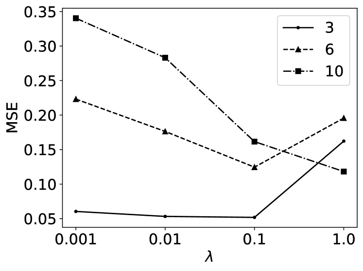
(a) $N=500$.

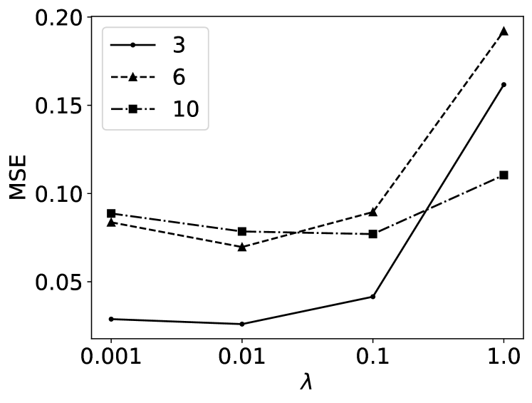
(b) $N=1000$.

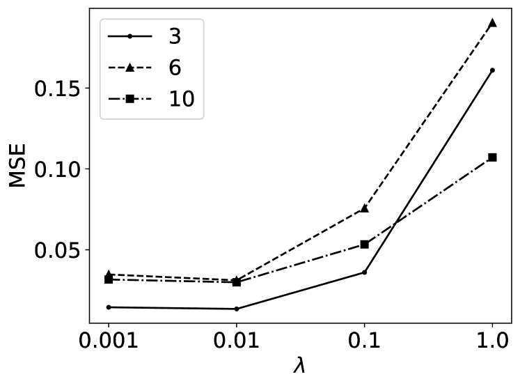
(c) $N=2000$.

Figure 1: Sensitivity Analysis for DGP-L.

(a) $N=500$.

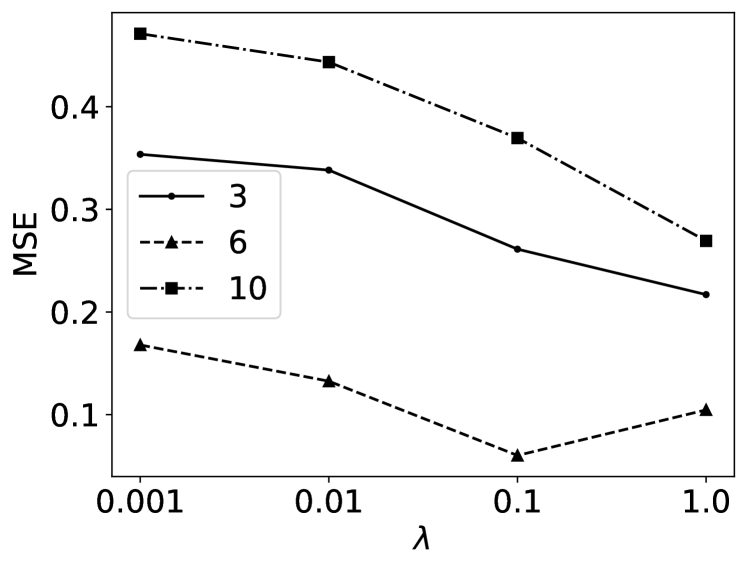
(b) $N=1000$.

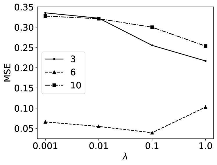
(c) $N=2000$.

Figure 2: Sensitivity Analysis for DGP-Q.

6.2 Orthogonal Series Ratio Estimator

Setting. As in the previous simulation, we consider CATE estimation by data combination, but now $H$ and $W$ depend on covariates. Therefore, simply applying DSR must result in biased estimation. We generate random samples of $O=(HY+(1-H)D,W,H,X)$ with a sample size $N=1000,2000,3000$ from the following DGP:

$$Y_{D}=\varsigma(\gamma^{\prime}X)+0.4D\gamma^{\prime}X+0.2\epsilon,$$

$$P(D_{1}=1|X)=\varsigma(0.2\gamma^{\prime}X+1),\hskip 14.22636ptP(D_{0}=1|X)=0,$$

$$P(W=1|X)=\varsigma(0.1\gamma^{\prime}X),\hskip 14.22636ptP(H=1|X)=\varsigma(-0.1\gamma^{\prime}X).$$

where $X=(X_{1},\ldots,X_{5})^{\prime}$ is a five-dimensional covariate vector with all elements having zero mean, and $\gamma$ is a five-dimensional vector with one in all elements. The covariance matrix of $X$ takes one for diagonal elements, and the absolute value of non-diagonal elements is randomly chosen from $[0.1,0.3]$ except that $X_{1}$ is independent of all the other covariates. The number of replication is set $1000$.

The estimand is CATE as a function of only the first covariate: $\theta_{0}(v)=E[Y_{1}-Y_{0}|X_{1}=v]=0.4v$. We use the polynomial basis up to the third order to construct OSR, and the order is selected based on 5-fold CV in each replication. ML estimators used for the nuisance estimation are random forest (RF), gradient boosting trees (GBT) and multi-layer perceptron (MLP). ML estimators are implemented using scikit-learn 1.0.2, and we use the default value for all options and hyperparameters. We use 5-fold cross-fitting to construct the orthogonal signals $\hat{U}$ and $\hat{T}$. Unlike the previous one, regularization is not employed in this simulation.

Table 5: Simulation Results for Orthogonal Series Estimator with Random Forest.

		$N=1000$				$N=2000$				$N=3000$
$q$		MSE	Bias	Width		MSE	Bias	Width		MSE	Bias	Width
0.2		0.005	-0.083	2.089		0.003	-0.047	1.449		0.002	-0.029	1.145
0.4		0.011	-0.011	2.667		0.005	0.000	1.725		0.004	0.008	1.317
0.6		0.020	0.051	3.637		0.009	0.042	2.308		0.006	0.041	1.590
0.8		0.038	0.130	7.665		0.016	0.092	4.497		0.010	0.081	3.327
Mean		0.096	0.023	48.238		0.027	0.024	9.691		0.012	0.028	5.250
STD		1.153	0.140	936.180		0.325	0.090	110.607		0.073	0.067	38.138
CVR		0.970				0.962				0.953

Table 6: Simulation Results for Orthogonal Estimator with Gradient Boosting Trees.

		$N=1000$				$N=2000$				$N=3000$
$q$		MSE	Bias	Width		MSE	Bias	Width		MSE	Bias	Width
0.2		0.009	-0.097	2.790		0.003	-0.026	1.476		0.002	-0.003	1.066
0.4		0.022	0.001	3.922		0.006	0.023	1.755		0.005	0.028	1.240
0.6		0.040	0.077	5.911		0.011	0.060	2.189		0.007	0.060	1.511
0.8		0.092	0.189	12.263		0.020	0.117	4.393		0.012	0.103	3.291
Mean		0.484	0.052	134.424		0.042	0.048	22.211		0.014	0.050	6.652
STD		7.181	0.286	2497.353		0.645	0.094	428.023		0.071	0.066	66.374
CVR		0.964				0.956				0.918

Table 7: Simulation Results for Orthogonal Estimator with Multi-Layer Perceptron.

		$N=1000$				$N=2000$				$N=3000$
$q$		MSE	Bias	Width		MSE	Bias	Width		MSE	Bias	Width
0.2		0.004	-0.020	1.485		0.002	0.002	1.026		0.002	0.010	0.819
0.4		0.008	0.037	1.821		0.005	0.036	1.217		0.004	0.038	0.931
0.6		0.014	0.080	2.402		0.007	0.070	1.481		0.006	0.060	1.116
0.8		0.025	0.134	4.661		0.013	0.109	3.588		0.009	0.095	2.466
Mean		0.712	0.061	843.500		0.015	0.058	15.306		0.010	0.054	6.776
STD		21.803	0.136	26423.507		0.079	0.070	209.077		0.047	0.056	58.231
CVR		0.922				0.916				0.905

Results. Table 5, 6 and 7 present the simulation results when using RF, GBT and MLP for the nuisance estimation, respectively. Bias in the tables denotes the estimation bias evaluated at $v=1$, Width is the largest width of the 95% uniform confidence band, and CVR is the empirical coverage of the 95% uniform confidence band, namely, the proportion of the times out of 1000 replications that the true target function $\theta_{0}(v)=0.4v$ is included in the estimated confidence band. In addition to mean and standard deviation, we report the $q$-quantiles of MSE, Bias and Width for $q=0.2,0.4,0.6,0.8$ because OSR produces rare but extremely inaccurate estimates. This instability may be due to the structure of the orthogonal signals, where the inverse of the estimated probability is included, and it has been pointed out in the literature (Singh and Sun, 2019; Chernozhukov et al., 2022c, b). Further discussion on this point can be found in Section 8.

The results diverge for the different ML methods when the sample size is small, but it seems that the methods for nuisance estimates have less impact on the performance of OSR as the sample size grows. The mean of MSE and the width of the confidence band get smaller as $N$ gets larger for all ML methods. Although the mean of bias remains almost the same across sample sizes, the standard deviation decreases, which also indicates that an increase in sample size stabilises the estimation. The empirical coverage is reasonably close to the nominal rate of 95% for all the cases with RF and when GBT is used with $N=1000,2000$. However, when using GBT with $N=3000$ and MLP with all the sample sizes, the empirical coverage deviates from the nominal coverage, possibly reflecting the slightly large bias and small width in these cases. The large bias in GBT and MLP may be due to the fixed hyperparameters. Although we used fixed hyperparameters to reduce the computational burden in this simulation, we could select hyperparameters based on CV in practice to lower the bias and obtain the confidence band with the correct coverage.

7 Empirical Example

In this section, we apply OSR to estimate a causal effect of participation in 401(k) on household assets.

Setting. In the US, 401(k) is an employer-sponsored personal pension program first implemented in 1978. It is tax-deferred to encourage household savings for their retirement. Data from the US Census Bureau’s 1991 Survey of Income and Program Participation (SIPP) has been used in Poterba et al. (1994, 1995) and many subsequent studies to examine the effect of 401(k) participation on household savings. The key technical challenge in estimating the causal effect of 401(k) participation is there are not enough covariates available in the SIPP data to explain the self-selected participation among those who are eligible to participate in 401(k). Poterba et al. (1994, 1995) argue that eligibility for the 401(k) program can be regarded as exogenous after conditioning on some important variables because whether an employer offered 401(k) would not affect people’s job selection at least at the time the program just started, but they would instead make a decision based on other aspects of the job such as salary. Adopting this argument, we can estimate LATE of 401(k) participation in household savings with 401(k) eligibility as IV and other variables related to job choice to control selection bias.

In this empirical example, we use the data analyzed in Chernozhukov and Hansen (2004) and Chernozhukov et al. (2018), consisting of samples of 9915 households with the reference person of 25-64 years old, and at least one member is employed but no one is self-employed. We use net financial assets —defined as the sum of IRA (Individual Retirement Account) balances, 401(k) balances, checking accounts, US saving bonds, other interest-earning accounts in financial institutions, other interest-earning assets, stocks, and mutual funds minus non-mortgage debt— as the outcome $Y$, a binary indicator for 401(k) eligibility as IV $Z$, and a binary indicator for 401(k) participation as the treatment $D$. The covariate vector $X$ used in this analysis includes age, income, family size, years of education, marital status, two-earner status, defined benefit pension status, IRA participation status, and home ownership status.

We conduct analyses based on the usual one-sample LATE estimation as in Example 3.1 and two-sample LATE estimation explained in Section A.3. The parameter of interest is LATE as a function of income. For two-sample LATE estimation, we generate a dataset indicator $H$ such that $P(H=1|X=x)=\varsigma(0.1\gamma^{\prime}\tilde{x})$, where $\tilde{x}$ is a vector of the covariates scaled so that the values fall within $[0,1]$. We use the polynomial basis and the order is selected based on CV from $k=1,2,3$. We use a relatively large number of partitions $G=20$ to mitigate the impact of random sample-splitting on the performance of OSR. GBT is used for nuisance estimation.

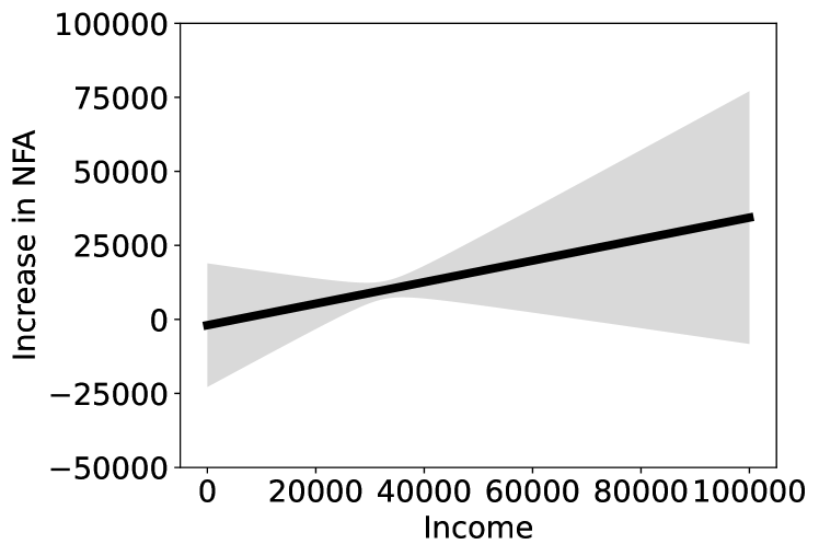
(a) One-Sample Estimation.

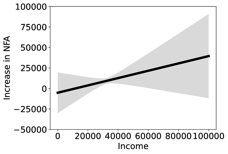
(b) Two-Sample Estimation.

Figure 3: Estimated LATE of 401(k) on Net Financial Assets Conditioned on Income Level and 95% Uniform Confidence Band.

Results. Figure 3(a) and (b) illustrate the estimated LATE function of income and its 95% uniform confidence band constructed by one-sample estimation and two-sample estimation, respectively. As can be seen, $k=1$ is selected in both one-sample and two-sample estimations. The estimated LATE is linearly increasing in household income and the slope is approximately 0.36 in one-sample estimation and 0.45 in two-sample estimation. Furthermore, the point estimate of LATE for households with annual income $50000 is $16225 in one-sample estimation and $17141 in two-sample estimation, which are consistent with the analysis in Ogburn et al. (2015) whose estimate is $14910. Statistically significant positive LATE is indicated for households with annual income $24000-$68000 in one-sample estimation, while LATE is significantly positive for households with income $26000-61000 in two-sample estimation, reflecting the wider confidence band in two-sample estimation.

8 Discussions

This section discusses the limitation and future direction of the present study. The first topic is model selection in the proposed framework. As explained in Remark 2.3, we can perform model selection based on CV using the criterion (4) only when $\zeta_{0}$ is strictly positive. We explained the several examples where $\zeta_{0}$ is necessarily positive, and it is shown in the simulation study in Section 6.1 that CV using the criterion (4) works well. However, there are also situations where $\zeta_{0}$ can take both positive and negative values, such as LATE estimation and IDID. Therefore, a model selection method for the general situation is key to increasing the practicality of the proposed framework. Despite its practical importance, little attention has been paid to model selection in the treatment effects estimation (Schuler et al., 2018; Caron et al., 2020). To the best of our knowledge, there exist only a few attempts in the literature to develop a flexible method for selecting the treatment effect model (Brookhart and van der Laan, 2006; Rolling and Yang, 2014; Saito and Yasui, 2020). Although we may be able to extend the ideas of these previous studies for the CEFR problems, further research on model selection is essential to enhance the feasibility of causal inference methods.

One of the drawbacks of the proposed framework is the large variability found in the simulation of Section 6.1. It may be due to the structure of the orthogonal signals, in which the inverse of the estimated propensity score is used. Inverse probability weighting (IPW) is known to suffer from unstable estimates especially when the propensity score is close to zero (Wooldridge, 2002, 2007; Robins et al., 2007; Seaman and White, 2013). This problem is especially acute in the data combination settings including two-sample estimation of LATE and IDID, where we have to perform four-class or eight-class classification to estimate propensity scores. Although we can increase stability by trimming small probabilities, determining the optimal threshold is nontrivial (Lee et al., 2011), and trimming can cause additional bias. Recently developed automatic debiased machine learning (Auto-DML) (Chernozhukov et al., 2022c) can be an effective solution to the problem because it avoids the estimation of propensity scores. Auto-DML directly estimates the Riesz representer of the orthogonal signals rather than constructing it with the inverse of the estimated propensity score. A much smaller variance of Auto-DML compared to the original DML has been empirically verified in numerical experiments (Singh and Sun, 2019; Chernozhukov et al., 2022b). Thus, extending the procedures and theory of the proposed framework to accommodate signals obtained by Auto-DML is a promising future direction.

The present study proposed a general and flexible framework for the CEFR problems, but more efficient estimation and inference may be possible in some specific settings. For example, the orthogonal moment condition for LATE using the interaction term of $Y$ and $D$ has been proposed in Singh and Sun (2019), while OSR uses $Y$ and $D$ only separately. Comparison of the efficiency of the method in Singh and Sun (2019) and OSR is beyond the scope of this study, but intuitively, leveraging information expressed in the form of interaction of $Y$ and $D$ can improve efficiency. However, the contribution of this study for offering the flexible inference framework in the data combination settings is significant, as the method in Singh and Sun (2019) is not applicable to situations where $Y$ and $D$ are separately observed.

Appendix A Additional Examples

A.1 Other Form of Ratio-Based Treatment Effects

Liang and Yu (2020) has proposed the other form of ratio-based treatment effects such as:

$$\theta_{0}(v)=\frac{E[Y_{1}-Y_{0}|V=v]}{E[Y_{1}+Y_{0}|V=v]}.$$

In this case, we need Assumption 5.3 but with $E[Y_{1}+Y_{0}|V=v]\neq 0$ for all $v\in\mathcal{V}$ instead of $E[Y_{0}|V=v]\neq 0$ for all $v\in\mathcal{V}$ for identification. We have that $\nu_{0}(v)=E[\mu_{0}(1,X)-\mu_{0}(0,X)|V=v]$ and $\zeta_{0}(v)=E[\mu_{0}(1,X)+\mu_{0}(0,X)|V=v]$, where $\mu_{0}(d,x)=E[Y|D=d,X=x]$. The following signals satisfy the Neyman orthogonality:

$$U(O,\eta_{0}) =\mu_{0}(1,X)-\mu_{0}(0,X)+\frac{D(Y-\mu_{0}(1,X))}{\pi_{0}(X)}-\frac{(1-D)(Y-\mu_{0}(0,X))}{1-\pi_{0}(X)},$$

$$T(O,\eta_{0}) =\mu_{0}(1,X)+\mu_{0}(0,X)+\frac{D(Y-\mu_{0}(1,X))}{\pi_{0}(X)}+\frac{(1-D)(Y-\mu_{0}(0,X))}{1-\pi_{0}(X)},$$

where $\pi_{0}(x)=E[D|X=x]$.

A.2 Ratio-Based LATE

We can also consider the ratio-based LATE, which is defined as:

$$\theta_{0}(v)=\frac{E[Y_{1}|D_{1}>D_{0},V=v]}{E[Y_{0}|D_{1}>D_{0},V=v]}.$$

If Assumption 5.1 in addition to $E[Y_{0}|D_{1}>D_{0},V=v]$ for $v\in\mathcal{V}$ hold, then

$$\theta_{0}(v)=\frac{E[E[DY|Z=1,X]-E[DY|Z=0,X]|V=v]}{E[E[(1-D)Y|Z=0,X]-E[(1-D)Y|Z=1,X]|V=v]}.$$

In this case, $\nu_{0}(v)=E[\mu_{0}(1,X)-\mu_{0}(0,X)|V=v]$ and $\zeta_{0}(v)=E[\pi_{0}(0,X)-\pi_{0}(1,X)|V=v]$, where $\mu_{0}(z,x)=E[DY|Z=z,X=x]$ and $\pi_{0}(z,x)=E[(1-D)Y|Z=z,X=x]$. The following signals satisfy the Neyman orthogonality:

$$U(O,\eta_{0}) =\mu_{0}(1,X)-\mu_{0}(0,X)+\frac{Z(DY-\mu_{0}(1,X))}{\rho_{0}(X)}-\frac{(1-Z)(DY-\mu_{0}(0,X))}{1-\rho_{0}(X)},$$

$$T(O,\eta_{0}) =\pi_{0}(0,X)-\pi_{0}(1,X)+\frac{(1-Z)((1-D)Y-\pi_{0}(0,X))}{1-\rho_{0}(X)}-\frac{Z((1-D)Y-\pi_{0}(1,X))}{\rho_{0}(X)},$$

where $\rho_{0}(x)=E[Z|X=x]$.

As in the previous subsection, we can consider the alternative form:

$$\theta_{0}(v)=\frac{E[Y_{1}-Y_{0}|D_{1}>D_{0},V=v]}{E[Y_{1}+Y_{0}|D_{1}>D_{0},V=v]}.$$

Under Assumption 5.1 and $E[Y_{1}+Y_{0}|D_{1}>D_{0},V=v]\neq 0$ for $v\in\mathcal{V}$, then

$$\theta_{0}(v)=\frac{E[E[Y|Z=1,X]-E[Y|Z=0,X]|V=v]}{E[E[(2D-1)Y|Z=1,X]-E[(2D-1)Y|Z=0,X]|V=v]}.$$

In this case, $\nu_{0}(v)=E[\mu_{0}(1,X)-\mu_{0}(0,X)|V=v]$ and $\zeta_{0}(v)=E[\pi_{0}(1,X)-\pi_{0}(0,X)|V=v]$, where $\mu_{0}(z,x)=E[Y|Z=z,X=x]$ and $\pi_{0}(z,x)=E[(2D-1)Y|Z=z,X=x]$. The following signals satisfy the Neyman orthogonality:

$$U(O,\eta_{0}) =\mu_{0}(1,X)-\mu_{0}(0,X)+\frac{Z(Y-\mu_{0}(1,X))}{\rho_{0}(X)}-\frac{(1-Z)(Y-\mu_{0}(0,X))}{1-\rho_{0}(X)},$$

$$T(O,\eta_{0}) =\pi_{0}(1,X)-\pi_{0}(0,X)+\frac{Z((2D-1)Y-\pi_{0}(1,X))}{\rho_{0}(X)}-\frac{(1-Z)((2D-1)Y-\pi_{0}(0,X))}{1-\rho_{0}(X)},$$

where $\rho_{0}(x)=E[Z|X=x]$.

A.3 Two-Sample LATE

It is obvious from the identification result of difference-based LATE that the two-sample estimation is possible. Let the observed vector be $O=(HY+(1-H)D,Z,H,X)$, where $H$ is a binary dataset indicator, and suppose that $Y_{1},Y_{0},D_{1},D_{0}\mathchoice{\mathrel{\hbox to0.0pt{$\displaystyle\perp$\hss}\mkern 2.0mu{\displaystyle\perp}}}{\mathrel{\hbox to0.0pt{$\textstyle\perp$\hss}\mkern 2.0mu{\textstyle\perp}}}{\mathrel{\hbox to0.0pt{$\scriptstyle\perp$\hss}\mkern 2.0mu{\scriptstyle\perp}}}{\mathrel{\hbox to0.0pt{$\scriptscriptstyle\perp$\hss}\mkern 2.0mu{\scriptscriptstyle\perp}}}H|X$ in addition to Assumption 5.1. Then, LATE is identified as:

$$\theta_{0}(v)=\frac{E[E[Y|H=1,Z=1,X]-E[Y|H=1,Z=0,X]|V=v]}{E[E[D|H=0,Z=1,X]-E[D|H=0,Z=0,X]|V=v]}.$$

In this case, $\nu_{0}(v)=E[\mu_{0}(1,X)-\mu_{0}(0,X)|V=v]$ and $\zeta_{0}(v)=E[\pi_{0}(1,X)-\pi_{0}(0,X)|V=v]$, where $\mu_{0}(z,x)=E[Y|H=1,Z=z,X=x]$ and $\pi_{0}(z,x)=E[D|H=0,Z=z,X=x]$. The following signals satisfy the Neyman orthogonality:

$$U(O,\eta_{0}) =\mu_{0}(1,X)-\mu_{0}(0,X)+\frac{HZ(Y-\mu_{0}(1,X))}{\rho_{0}(1,1,X)}-\frac{H(1-Z)(Y-\mu_{0}(0,X))}{\rho_{0}(1,0,X)},$$

$$T(O,\eta_{0}) =\pi_{0}(1,X)-\pi_{0}(0,X)+\frac{(1-H)Z(D-\pi_{0}(1,X))}{\rho_{0}(0,1,X)}-\frac{(1-H)(1-Z)(D-\pi_{0}(0,X))}{\rho_{0}(0,0,X)},$$

where $\rho_{0}(h,z,x)=P(H=h,Z=z|X=x)$.

Although two-sample LATE estimation is similar to the data combination in Example 3.4, they are different in the observed variables and the underlying assumptions. The significant difference is that we must observe $Z$ in two-sample LATE estimation, whereas we only need to know that the treatment regimes $P(Z_{w}=1|X)$ are different according to $w$ in Example 3.4.

A.4 Two-Sample IDID

As shown in Ye et al. (2022), two-sample estimation is also possible in the IDID setting. The observable can be expressed as $O=(HY+(1-H)D,Z,W,H,X)$. If $D_{zw},Y_{1w}-Y_{0w},Y_{01}-Y_{00}\mathchoice{\mathrel{\hbox to0.0pt{$\displaystyle\perp$\hss}\mkern 2.0mu{\displaystyle\perp}}}{\mathrel{\hbox to0.0pt{$\textstyle\perp$\hss}\mkern 2.0mu{\textstyle\perp}}}{\mathrel{\hbox to0.0pt{$\scriptstyle\perp$\hss}\mkern 2.0mu{\scriptstyle\perp}}}{\mathrel{\hbox to0.0pt{$\scriptscriptstyle\perp$\hss}\mkern 2.0mu{\scriptscriptstyle\perp}}}H|X$ for $w,z=0,1$, then CATE is identified as:

$$\theta_{0}(v)=\frac{E[\mu_{0}(1,1,X)-\mu_{0}(0,1,X)-\mu_{0}(1,0,X)+\mu_{0}(0,0,X)|V=v]}{E[\pi_{0}(1,1,X)-\pi_{0}(0,1,X)-\pi_{0}(1,0,X)+\pi_{0}(0,0,X)|V=v]},$$

where $\mu_{0}(z,x)=E[Y|H=1,W=w,Z=z,X=x]$ and $\pi_{0}(z,x)=E[D|H=0,W=w,Z=z,X=x]$. In this case,

$$\nu_{0}(v) =\sum_{w,z\in\{0,1\}^{2}}(-1)^{w+z}E[\mu_{0}(w,z,X)|V=v],$$

$$\nu_{0}(v) =\sum_{w,z\in\{0,1\}^{2}}(-1)^{w+z}E[\pi_{0}(w,z,X)|V=v].$$

The following signals satisfy the Neyman orthogonality:

$$U(O,\eta_{0}) =\sum_{w,z\in\{0,1\}^{2}}(-1)^{w+z}\left(\mu_{0}(w,z,X)+\frac{1_{H=1}1_{W=w}1_{Z=z}(Y-\mu_{0}(w,z,X))}{\rho_{0}(1,w,z,X)}\right),$$

$$T(O,\eta_{0}) =\sum_{w,z\in\{0,1\}^{2}}(-1)^{w+z}\left(\pi_{0}(w,z,X)+\frac{1_{H=0}1_{W=w}1_{Z=z}(D-\pi_{0}(w,z,X))}{\rho_{0}(0,w,z,X)}\right),$$

where $\rho_{0}(h,w,z,x)=P(H=h,W=w,Z=z|X=x)$. We can obtain the estimate $\hat{\rho}(h,w,z,x)$ by implementing an eight-class classification. However, it becomes easier for $\hat{\rho}(h,w,z,x)$ to take small values as the number of classes increases, leading to the unstable estimation in practice.

Appendix B Proofs

B.1 Proofs of Results in Section 4

Lemma B.1 (LLN for Matrices).

Let $Q_{i},i\in[N]$ be independent not necessarily identically distributed and symmetric non-negative $K\times K$ matrices such that $K\geq 2$ and $\|Q_{i}\|\leq M$ $a.s.$ Let $Q=E_{N}[E[Q_{i}]]$ and $\hat{Q}=E_{N}[Q_{i}]$. Then,

$$E[\|\hat{Q}-Q\|]\leq\sqrt{\frac{M(1+\|Q\|)\log N}{N}}.$$

In particular, if $Q_{i}=p_{i}p_{i}^{\prime}t_{i}$ with $\|p_{i}\|\leq\xi_{k}$ and $|t_{i}|\leq 1$, then

$$E[\|\hat{Q}-Q\|]\leq\sqrt{\frac{\xi_{k}^{2}(1+\|Q\|)\log N}{N}}.$$

See Rudelson (1999); Tropp (2015); Belloni et al. (2015) for the proof.

Lemma B.2.

Let Assumption 4.1 and 4.5 hold. Then, all eigenvalues of $Q=E[p(V)p(V)^{\prime}\zeta_{0}(V)]$ are bounded above and away from zero uniformly over $k$.

Proof of Lemma B.2.

Define $\underline{\zeta}^{2}:=\inf_{v\in\mathcal{V}}\zeta_{0}(v)^{2}$. For any $a\in\{a\in\mathbb{R}^{k}:\|a\|\neq 0\|\}$,

$$(a^{\prime}E[p(V)p(V)^{\prime}\zeta_{0}(V)]a)^{2} =E[(a^{\prime}p(V))^{2}\zeta(V)]^{2}\geq E[(a^{\prime}p(V))^{2}]^{2}\underline{\zeta}^{2}>0.$$

The last inequality follows from $E[(a^{\prime}p(V))^{2}]>0$ Assumption 4.1 and $\underline{\zeta}^{2}>0$ by Assumption 4.5. ∎

Lemma B.3 (No Effect of First-Stage Error).

Under Assumption 4.6,

$$\sqrt{N}\|E_{N}[p_{i}(U_{i}(\hat{\eta})-U_{i}(\eta_{0}))]\| =O_{P}(B_{N}+\Lambda_{N})=o(1),$$

$$\sqrt{N}\|E_{N}[p_{i}(T_{i}(\hat{\eta})-T_{i}(\eta_{0}))]\| =O_{P}(B_{N}+\Lambda_{N})=o(1).$$

Proof of Lemma B.3.

Lemma B.3 follows from Assumption 4.6 and the proof of Lemma A.3 in Semenova and Chernozhukov (2021). ∎

Proof of Lemma 4.1.

(a) By Assumption 4.2 and Lemma B.1, $\|\hat{Q}-Q\|\rightarrow_{P}0$ as $N\rightarrow\infty$. Therefore, all eigenvalues of $\hat{Q}$ are also bounded away from zero with probability approaching one by Lemma B.2. Thus,

$$\|\hat{\beta}-\beta_{k}\| =\|\hat{Q}^{-1}E_{N}[p_{i}\hat{U}_{i}]-\beta_{0}\|=\|\hat{Q}^{-1}E_{N}[p_{i}(\hat{U}_{i}-\hat{T}_{i}\theta_{ki})]\|\lesssim\|E_{N}[p_{i}(\hat{U}_{i}-\hat{T}_{i}\theta_{ki})]\|.$$

We can decompose the estimated orthogonal scores as:

$$\hat{U}=(\hat{U}-U_{0})+\nu_{0}+\varepsilon_{U},\hskip 14.22636pt\hat{T}=(\hat{T}-T_{0})+\zeta_{0}+\varepsilon_{T}.$$

Using this decomposition and noting that $\theta_{k}=\theta_{0}-r$, we have

$$E_{N}[p_{i}(\hat{U}_{i}-\hat{T}_{i}\theta_{ki})] =E_{N}[p_{i}(\hat{U}_{i}-U_{0i})]+E_{N}[p_{i}\theta_{ki}(\hat{T}_{i}-T_{0i})]$$

$$\qquad+E_{N}[p_{i}\varepsilon_{Ui}]-E_{N}[p_{i}\theta_{0i}\varepsilon_{Ti}]+E_{N}[p_{i}\zeta_{0i}r_{i}]+E_{N}[p_{i}\varepsilon_{Ti}r_{i}]$$

$$=:J_{1}+J_{2}+J_{3}-J_{4}+J_{5}+J_{6}.$$

Therefore, it suffices to derive the bound on the norm of these six terms by the triangle inequality.

The first-stage errors $J_{1}$ and $J_{2}$ are bounded as

$$\|J_{1}\|+\|J_{2}\| \leq\|E_{N}[p_{i}(\hat{U}_{i}-U_{0i})]\|+\|E_{N}[p_{i}\theta_{0i}(\hat{T}_{i}-T_{0i})]\|+\|E_{N}[p_{i}r_{i}(\hat{T}_{i}-T_{0i})]\|$$

$$=o_{P}(N^{-1/2}(1+l_{k}r_{k})),$$

by Lemma B.3, Assumption 4.3 and Assumption 4.5. For $J_{3}$ and $J_{4}$, we have

$$\|J_{3}\|+\|J_{4}\|\lesssim\|E_{N}[p_{i}\varepsilon_{i}]\|$$

since $\theta_{0}=\nu_{0}/\zeta_{0}$ is uniformly bounded by Assumption 4.5. Similarly for $J_{5}$ and $J_{6}$, we have

$$\|J_{5}\|+\|J_{6}\|\lesssim\|E_{N}[p_{i}r_{i}]\|$$

by Assumption 4.4 and 4.5. As shown in the proof of Theorem 4.1 in Belloni et al. (2015), the bound is given as

$$\|E_{N}[p_{i}\varepsilon_{i}]\|+\|E_{N}[p_{i}r_{i}]\|\lesssim_{P}\sqrt{\frac{k}{N}}+\left(\sqrt{\frac{k}{N}}l_{k}r_{k}\land\frac{\xi_{k}r_{k}}{\sqrt{N}}\right).$$

This completes the proof of Lemma 4.1 (a).

(b) Using the same decomposition as in part (a), we obtain

$$\sqrt{N}\alpha^{\prime}(\hat{\beta}-\beta_{0}) =\sqrt{N}\alpha^{\prime}\hat{Q}^{-1}(J_{1}+J_{2}+J_{3}-J_{4}+J_{5}+J_{6})$$

$$=\alpha^{\prime}Q^{-1}\mathbb{G}_{N}[p_{i}(\varepsilon_{Ui}-\theta_{0i}\varepsilon_{Ti})]+\alpha^{\prime}(\hat{Q}^{-1}-Q^{-1})\mathbb{G}_{N}[p_{i}(\varepsilon_{Ui}-\theta_{0i}\varepsilon_{Ti})]$$

$$\qquad+\sqrt{N}\alpha^{\prime}Q^{-1}(J_{1}+J_{2})+\sqrt{N}\alpha^{\prime}(\hat{Q}^{-1}-Q^{-1})(J_{1}+J_{2})$$

$$\qquad+\sqrt{N}\alpha^{\prime}Q^{-1}(J_{5}+J_{6})+\sqrt{N}\alpha^{\prime}(\hat{Q}^{-1}-Q^{-1})(J_{5}+J_{6})$$

$$=:\alpha^{\prime}Q^{-1}\mathbb{G}_{N}[p_{i}(\varepsilon_{Ui}-\theta_{0i}\varepsilon_{Ti})]+L_{1}+L_{2}+L_{3}+L_{4}+L_{5}$$

$$=:\alpha^{\prime}Q^{-1}\mathbb{G}_{N}[p_{i}(\varepsilon_{Ui}-\theta_{0i}\varepsilon_{Ti})]+R_{N}(\alpha).$$

By Assumption 4.5, we have that

$$|L_{1}|\lesssim|\alpha^{\prime}(\hat{Q}^{-1}-Q^{-1})\mathbb{G}_{N}[p_{i}\varepsilon_{i}]|.$$

and its bound can be obtained as

$$|\alpha^{\prime}(\hat{Q}^{-1}-Q^{-1})\mathbb{G}_{N}[p_{i}\varepsilon_{i}]|\lesssim_{P}\sqrt{\frac{\xi_{k}^{2}\log N}{N}},$$

by the proof of Lemma 4.1 in Belloni et al. (2015). By Lemma B.1, B.2, B.3 and Assumption 4.2,

$$|L_{2}| \lesssim_{P}\|\alpha\|\|Q^{-1}\|\|\sqrt{N}(J_{1}+J_{2})\|=o(1),$$

$$|L_{3}| \lesssim_{P}\|\alpha\|\|\hat{Q}^{-1}-Q^{-1}\|\|\sqrt{N}(J_{1}+J_{2})\|\lesssim_{P}\sqrt{\frac{\xi_{k}^{2}\log N}{N}}o(1)=o(1).$$

For $|L_{4}|$, we have that

$$|L_{4}| \lesssim\left|\sqrt{N}E_{N}[\alpha^{\prime}p_{i}r_{i}]\right|\lesssim_{P}E[(\alpha^{\prime}p_{i}r_{i})^{2}]^{1/2}\lesssim l_{k}r_{k},$$

where the first wave inequality follows from Assumption 4.4 and 4.5, the second inequality follows from Chebyshev’s inequality since $E[p_{i}r_{i}]=0$, and the last wave inequality follows from Assumption 4.3. Also, for $|L_{5}|$, we have that

$$|L_{5}| \lesssim\left\|\hat{Q}^{-1}-Q^{-1}\right\|\left\|\sqrt{N}E_{N}[p_{i}r_{i}]\right\|\lesssim_{P}\sqrt{\frac{\xi_{k}^{2}\log N}{N}}\left(l_{k}r_{k}\sqrt{k}\land\xi_{k}r_{k}\right),$$

which is shown in the proof of Lemma 4.1 in Belloni et al. (2015). Combining the bounds on $L_{j}$ for $j\in[5]$ gives the linearization result. ∎

Proof of Theorem 4.1.

Theorem 4.1 can be proved by using Lemma 4.1 and applying the proof of Theorem 4.2 in Belloni et al. (2015). ∎

Proof of Lemma 4.2.

(a) The similar decomposition as in the proof of Lemma 4.1 (b) gives

$$R_{N}(\alpha(v)) =\alpha(v)^{\prime}(\hat{Q}^{-1}-Q^{-1})\mathbb{G}_{N}[p_{i}(\varepsilon_{Ui}+\theta_{0i}\varepsilon_{Ti})]$$

$$\qquad+\sqrt{N}\alpha(v)^{\prime}Q^{-1}(J_{1}+J_{2})+\sqrt{N}\alpha(v)^{\prime}(\hat{Q}^{-1}-Q^{-1})(J_{1}+J_{2})$$

$$\qquad+\sqrt{N}\alpha(v)^{\prime}Q^{-1}(J_{5}+J_{6})+\sqrt{N}\alpha(v)^{\prime}(\hat{Q}^{-1}-Q^{-1})(J_{5}+J_{6})$$

$$=:L_{1}(v)+L_{2}(v)+L_{3}(v)+L_{4}(v)+L_{5}(v).$$

By the similar argument as in the proof of Lemma 4.1 (b), we have that

$$|L_{1}(v)|\lesssim\left|\alpha(v)^{\prime}(\hat{Q}^{-1}-Q^{-1})\mathbb{G}_{N}[p_{i}\varepsilon_{i}]\right|.$$

According to the proof of Lemma 4.2 in Belloni et al. (2015),

$$\sup_{v\in\mathcal{V}}\left|\alpha(v)^{\prime}(\hat{Q}^{-1}-Q^{-1})\mathbb{G}_{N}[p_{i}\varepsilon_{i}]\right|\lesssim_{P}N^{1/m}\sqrt{\frac{\xi_{k}^{2}\log^{2}N}{N}}.$$

By Lemma B.1, B.2, B.3 and Assumption 4.2,

$$\sup_{v\in\mathcal{V}}|L_{2}(v)| \leq\sup_{v\in\mathcal{V}}\|\alpha(v)\|\left\|Q^{-1}\right\|\left\|\sqrt{N}(J_{1}+J_{2})\right\|=o(1),$$

$$\sup_{v\in\mathcal{V}}|L_{3}(v)| \leq\sup_{v\in\mathcal{V}}\|\alpha(v)\|\left\|\hat{Q}^{-1}-Q^{-1}\right\|\left\|\sqrt{N}(J_{1}+J_{2})\right\|\lesssim_{P}\sqrt{\frac{\xi_{k}^{2}\log N}{N}}o(1)=o(1).$$

For $L_{4}(v)$ and $L_{5}(v)$, we have that

$$\sup_{v\in\mathcal{V}}|L_{4}(v)| \lesssim\sup_{v\in\mathcal{V}}\left|\sqrt{N}\alpha(v)^{\prime}Q^{-1}E_{N}[p_{i}r_{i}]\right|\lesssim_{P}l_{k}r_{k}\sqrt{\log k},$$

$$\sup_{v\in\mathcal{V}}|L_{5}(v)| \lesssim\sup_{v\in\mathcal{V}}\left|\sqrt{N}\alpha(v)^{\prime}(\hat{Q}^{-1}-Q^{-1})E_{N}[p_{i}r_{i}]\right|\lesssim_{P}\sqrt{\frac{\xi_{k}^{2}\log N}{N}}\left(l_{k}r_{k}\sqrt{k}\land\xi_{k}r_{k}\right),$$

where the first inequality in both lines follows from Assumption 4.4 and 4.5, and the both bounds are given by Lemma 4.2 in Belloni et al. (2015). Combining the bounds on $L_{j}(v)$ for $j\in[5]$ gives the linearization result.

(b) Lemma 4.2 (b) follows from Lemma 4.2 (a) and the proof of Theorem 4.3 in Belloni et al. (2015). ∎

Proof of Theorem 4.2.

Theorem 4.2 can be proved by using Lemma 4.2 and applying the proof of Theorem 4.4 in Belloni et al. (2015). ∎

Proof of Theorem 4.3.

Theorem 4.3 can be proved by applying the proof of Theorem 3.3 in Semenova and Chernozhukov (2021). ∎

Proof of Theorem 4.4.

Theorem 4.4 follows from the proof of Theorem 3.4 in Semenova and Chernozhukov (2021). See also Chernozhukov et al. (2013) for details. ∎

Proof of Theorem 4.5.

Theorem 4.5 follows from the proof of Theorem 3.5 in Semenova and Chernozhukov (2021). See also Belloni et al. (2015) for details. ∎

B.2 Proofs of Results in Section 5

Lemma B.4 (Neyman Orthogonality of the Doubly Robust Signal).

Consider the following doubly robust type signal:

$$U(O,\eta_{0}) =\mu_{0}(1,X)+\frac{Z(Y-\mu_{0}(1,X))}{\rho_{0}(X)},$$

where $Z$ is a binary variable, $\mu_{0}(z,x)=E[Y|Z=z,X=x]$ is an outcome regression function and $\rho_{0}(x)=E[Z|X=x]$ is a propensity score. Also, define $\nu_{0}(v)=E[\mu_{0}(1,X)|V=v]$. Then, the above signal satisfies the Neyman orthogonality, namely, for all $v\in\mathcal{V}$,

$$\partial_{s}E[U(O,\eta_{0}+s(\eta-\eta_{0}))-\nu_{0}(V)|V=v]|_{s=0}=0.$$

Proof of Lemma B.4.

If we can interchange differentiation and integration, we have, for $\Psi(s):=\partial_{s}E[U(O,\eta_{0}+s(\eta-\eta_{0}))-\nu_{0}(V)|V=v]$, that

$$\Psi(s) =\partial_{s}E\left[\left.s(\mu-\mu_{0})-\frac{s\rho_{0}(\mu-\mu_{0})}{\rho_{0}+s(\rho-\rho_{0})}\right|V\right]$$

$$=E\left[\left.\mu-\mu_{0}-\frac{\rho_{0}(\mu-\mu_{0})(\rho_{0}+s(\rho-\rho_{0}))-s\rho_{0}(\mu-\mu_{0})(\rho-\rho_{0})}{(\rho_{0}+s(\rho-\rho_{0}))^{2}}\right|V\right]$$

$$=E\left[\left.\mu-\mu_{0}-\frac{\rho_{0}^{2}(\mu-\mu_{0})}{(\rho_{0}+s(\rho-\rho_{0}))^{2}}\right|V\right].$$

Thus, $\Psi(0)=0$, which concludes the proof. ∎

Proof of Theorem 5.1.

(a) We have that

$$\nu_{0}(v) =E[D_{1}Y_{1}+(1-D_{1})Y_{0}|V=v]-E[D_{0}Y_{1}+(1-D_{0})Y_{0}|V=v]$$

$$=E[(D_{1}-D_{0})(Y_{1}-Y_{0})|V=v]$$

$$=E[D_{1}-D_{0}|V=v]E[Y_{1}-Y_{0}|D_{1}-D_{0}=1,V=v],$$

where the first equality holds by Assumption 5.1.1, and the last inequality follows from that $D_{1}-D_{0}\in\{0,1\}$ by Assumption 5.1.4. Likewise, we have that

$$\zeta_{0}(v) =E[D_{1}-D_{0}|V=v],$$

by Assumption 5.1.1. Lastly, because $E[D_{1}-D_{0}|V=v]\neq 0$ for all $v\in\mathcal{V}$ by Assumption 5.1.3, $\nu_{0}(v)/\zeta_{0}(v)$ is well-defined and it equals to

$$\frac{\nu_{0}(v)}{\zeta_{0}(v)} =\frac{E[D_{1}-D_{0}|V=v]E[Y_{1}-Y_{0}|D_{1}-D_{0}=1,V=v]}{E[D_{1}-D_{0}|V=v]}$$

$$=E[Y_{1}-Y_{0}|D_{1}>D_{0},V=v]$$

$$=\theta_{0}(v),$$

where the second equality holds since $D_{1}-D_{0}=1$ implies that $D_{1}>D_{0}$.

(b) The moment conditions in part (b) immediately follow from the definition of the regression functions $\mu_{0},\pi_{0}$ and the propensity score $\rho_{0}$.

(c) The Neyman orthogonality of the signals $U$ and $T$ follows from Lemma B.4. ∎

Proof of Corollary 5.1.

We can decompose $U(O,\eta)-U(O,\eta_{0})$ as

$$U(O,\eta)-U(O,\eta_{0}) =(\mu(1,X)-\mu_{0}(1,X))\left(1-\frac{Z}{\rho_{0}(X)}\right)-(\mu(0,X)-\mu_{0}(0,X))\left(1-\frac{1-Z}{1-\rho_{0}(X)}\right)$$

$$\quad+(\rho_{0}(X)-\rho(X))(Y-\mu_{0}(1,X))\frac{Z}{\rho(X)\rho_{0}(X)}$$

$$\qquad-(\rho_{0}(X)-\rho(X))(Y-\mu_{0}(0,X))\frac{1-Z}{(1-\rho(X))(1-\rho_{0}(X))}$$

$$\quad+(\rho_{0}(X)-\rho(X))(\mu_{0}(1,X)-\mu(1,X))\frac{D}{\rho(X)\rho_{0}(X)}$$

$$\qquad-(\rho_{0}(X)-\rho(X))(\mu_{0}(0,X)-\mu(0,X))\frac{1-D}{(1-\rho(X))(1-\rho_{0}(X))}$$

$$=:S_{1}+S_{1}^{\prime}+S_{2}+S_{2}^{\prime}+S_{3}+S_{3}^{\prime}.$$

In what follows, we will bound $S_{1}$, $S_{2}$ and $S_{3}$ as the bounds on $S_{1}^{\prime}$, $S_{2}^{\prime}$ and $S_{3}^{\prime}$ follow from a similar argument.

Bound on $B_{N}$. By the law of iterated expectation, we have

$$E[p(V)S_{1}]=E\left[p(V)(\mu(1,X)-\mu_{0}(1,X))E\left[\left.1-\frac{Z}{\rho_{0}(X)}\right|X\right]\right]=0,$$

and likewise,

$$E[p(V)S_{2}]=E\left[p(V)\frac{\rho_{0}(X)-\rho(X)}{\rho(X)\rho_{0}(X)}E[Z(Y-\mu_{0}(1,X))|X]\right]=0.$$

For $S_{3}$, we have that

$$\|E[p(V)S_{3}]\|^{2}\leq\overline{C}^{3}\|E[p(V)(\rho_{0}(X)-\rho(X))(\mu_{0}(1,X)-\mu(1,X))]\|^{2},$$

where we use the fact that

$$E[Z^{2}\rho(X)^{-2}\rho_{0}(X)^{-2}|X]=E[Z|X]\rho(X)^{-2}\rho_{0}(X)^{-2}\leq\overline{C}^{3}.$$ (10)

Therefore, for the case of bounded basis, we can bound $\|E[p(V)S_{3}]\|^{2}$ as

$$\|E[p(V)S_{3}]\|^{2} \lesssim\|E[p(V)(\rho_{0}(X)-\rho(X))(\mu_{0}(1,X)-\mu(1,X))]\|^{2}$$

$$\lesssim\sum_{j=1}^{k}E[p_{j}(V)(\rho_{0}(X)-\rho(X))(\mu_{0}(1,X)-\mu(1,X))]^{2}$$

$$\leq k\mathbf{m}_{N,2}^{2}\mathbf{r}_{N,2}^{2},$$

where the last inequality follows by Cauchy–Schwarz inequality. Since the same bound can be derived for $S_{1}^{\prime}$, $S_{2}^{\prime}$ and $S_{3}^{\prime}$, it follows that

$$\|E[p(V)(U-U_{0})]\|\lesssim\sqrt{k}\mathbf{m}_{N,2}\mathbf{r}_{N,2}.$$

The almost same argument derives the bound

$$\|E[p(V)(T-T_{0})]\|\lesssim\sqrt{k}\mathbf{p}_{N,2}\mathbf{r}_{N,2}.$$

since the signals $U$ and $T$ have the same structure. Thus, we have that

$$B_{N}\lesssim\sqrt{kN}\mathbf{r}_{N,2}(\mathbf{m}_{N,2}+\mathbf{p}_{N,2})=o(1).$$

When the basis is not bounded, we can alternatively bound $\|E[p(V)S_{3}]\|^{2}$ as

$$\|E[p(V)S_{3}]\|^{2} \lesssim\|E[p(V)(\rho_{0}(X)-\rho(X))(\mu_{0}(1,X)-\mu(1,X))]\|^{2}$$

$$\lesssim\sum_{j=1}^{k}E[p_{j}(V)(\rho_{0}(X)-\rho(X))^{2}(\mu_{0}(1,X)-\mu(1,X))^{2}]^{2}$$

$$\leq k\mathbf{m}_{N,2\omega}^{2}\mathbf{r}_{N,2\psi}^{2},$$

where the last inequality follows by Hölder’s inequality. Likewise in the case of bounded basis, we have for unbounded basis that

$$B_{N}\lesssim\sqrt{kN}\mathbf{r}_{N,2\psi}(\mathbf{m}_{N,2\omega}+\mathbf{p}_{N,2\omega^{\prime}})=o(1).$$

Bound on $\Lambda_{N}$. It suffices to derive the bounds on $E[S_{j}^{2}]$ for $j=1,2,3$ since

$$\Lambda_{N}\lesssim\xi_{k}\left(\sup_{\eta\in\mathcal{S}_{N}}E\left[(U-U_{0})^{2}\right]^{1/2}\lor\sup_{\eta\in\mathcal{S}_{N}}E\left[(T-T_{0})^{2}\right]^{1/2}\right),$$ (11)

by definition. We have that

$$E[S_{1}^{2}]=E\left[(\mu(1,X)-\mu_{0}(1,X))^{2}E\left[(1-Z\rho_{0}(X)^{-1})^{2}|X\right]\right]\lesssim\overline{C}\mathbf{m}_{N,2}^{2},$$

where the wave inequality is implied by

$$E\left[(1-Z\rho_{0}(X)^{-1})^{2}|X\right]=1-2+\rho_{0}(X)^{-1}\leq\overline{C}.$$

By (10), we have that

$$E[S_{2}^{2}]=E\left[(\rho_{0}(X)-\rho(X))^{2}E\left[(Y-\mu_{0}(1,X))^{2}|Z=1,X\right]\rho(X)^{-2}\rho_{0}(X)^{-1}\right]\lesssim\overline{C}^{3}\mathbf{r}_{N,2}^{2}.$$

Lastly, $E[S_{3}^{2}]$ is bounded as

$$E[S_{3}^{2}]=E\left[(\rho_{0}(X)-\rho(X))^{2}(\mu(1,X)-\mu_{0}(1,X))^{2}\rho(X)^{-2}\rho_{0}(X)^{-1}\right]\leq\overline{C}^{5}(\mathbf{m}_{N,2}^{2}\land\mathbf{r}_{N,2}^{2}),$$

because we can bound the terms $(\rho_{0}(X)-\rho(X))^{2}$ and $(\mu(1,X)-\mu_{0}(1,X))^{2}$ by $\overline{C}^{2}$. Thus, Assumption 5.2, (11) and the bounds on $E[S_{j}^{2}]$ for $j=1,2,3$ gives

$$\sup_{\eta\in\mathcal{S}_{N}}E\left[\|p(V)(U-U_{0})\|^{2}\right]^{1/2}\lesssim\xi_{k}(\mathbf{m}_{N,2}\lor\mathbf{r}_{N,2}).$$

Combining this result with the bound on $\sup_{\eta\in\mathcal{S}_{N}}E\left[\|p(V)(T-T_{0})\|^{2}\right]^{1/2}$ gives $\Lambda_{N}\lesssim\xi_{k}(\mathbf{m}_{N,2}\lor\mathbf{p}_{N,2}\lor\mathbf{r}_{N,2})=o(1)$, which concludes the proof. ∎

Proof of Theorem 5.2.

(a) We have that $\mu_{0}(d,x)=E[Y_{d}|X=x]$ by Assumption 5.3.1 and 5.3.4. Therefore, $\nu_{0}(v)=E[\mu_{0}(1,X)|V=v]=E[Y_{1}|V=v]$ and $\zeta_{0}(v)=E[\mu_{0}(0,X)|V=v]=E[Y_{0}|V=v]$, which together with Assumption 5.3.3 indicates $\theta_{0}(v)=\nu_{0}(v)/\zeta_{0}(v)$.

(b) The moment conditions in part (b) immediately follow from the definition of the regression functions $\mu_{0}$ and the propensity score $\pi_{0}$.

(c) The Neyman orthogonality of the signals $U$ and $T$ follows from Lemma B.4. ∎

Proof of Corollary 5.2.

The same arguments in the proof of Corollary 5.1 can be used to derive $B_{N}\lesssim\sqrt{kN}\mathbf{m}_{N,2}\mathbf{p}_{N,2}=o(1)$ for bounded basis, $B_{N}\lesssim\sqrt{kN}\mathbf{m}_{N,2\omega}\mathbf{p}_{N,2\psi}=o(1)$ for unbounded basis, and $\Lambda_{N}\lesssim\xi_{k}(\mathbf{m}_{N,2}\lor\mathbf{p}_{N,2})=o(1)$. ∎

Proof of Theorem 5.3.

(a) For $z=0,1$, we have that

$$\mu_{0}(1,z,X)-\mu_{0}(0,z,X) =E[D_{z1}(Y_{11}-Y_{01})+Y_{01}-D_{z0}(Y_{10}+Y_{00})-Y_{00}|Z=z,X]$$

$$=E[D_{z1}(Y_{11}-Y_{01})-D_{z0}(Y_{10}+Y_{00})|X]+E[Y_{01}-Y_{00}|X],$$

where the first equality follows by Assumption 5.5.1 and 3, and the second equality follows by Assumption 5.5.5. Therefore,

$$\sum_{(w,z)\in\{0,1\}^{2}}(-1)^{w+z}\mu_{0}(w,z,X) =E[(D_{11}-D_{01})(Y_{11}-Y_{01})-(D_{10}-D_{00})(Y_{10}+Y_{00})|X]$$

$$=E[D_{11}-D_{01}-D_{10}+D_{00}|X]E[Y_{1}-Y_{0}|X],$$

where the second equality follows by Assumption 5.5.6 and 7. Moreover, we have that

$$\sum_{(w,z)\in\{0,1\}^{2}}(-1)^{w+z}\pi_{0}(w,z,X)=E[D_{11}-D_{01}-D_{10}+D_{00}|X],$$

by Assumption 5.5.1, 3, 4 and 5. Combining these results show that $\theta_{0}(v)=\nu_{0}(v)/\zeta_{0}(v)$.

(b) The moment conditions in part (b) immediately follow from the definition of the regression functions $\mu_{0},\pi_{0}$ and the propensity score $\rho_{0}$.

(c) The Neyman orthogonality of the signals $U$ and $T$ follows from Lemma B.4. ∎

Proof of Corollary 5.3.

The same arguments in the proof of Corollary 5.1 can be used to derive $B_{N}\lesssim\sqrt{kN}\mathbf{r}_{N,2}(\mathbf{m}_{N,2}+\mathbf{p}_{N,2})=o(1)$ for bounded basis, $B_{N}\lesssim\sqrt{kN}(\mathbf{m}_{N,2\omega}\mathbf{r}_{N,2\psi}+\mathbf{p}_{N,2\omega^{\prime}}\mathbf{r}_{N,2\psi^{\prime}})=o(1)$ for unbounded basis, and $\Lambda_{N}\lesssim\xi_{k}(\mathbf{m}_{N,2}\lor\mathbf{p}_{N,2}\lor\mathbf{r}_{N,2})=o(1)$. ∎

Proof of Theorem 5.4.

(a) First, we provide the proof for LATE. We have that

$$\mu_{0}(1,X)-\mu_{0}(0,X) =E[(Z_{1}-Z_{0})(D_{1}-D_{0})(Y_{1}-Y_{0})|X]$$

$$=E[Z_{1}-Z_{0}|X]E[D_{1}-D_{0}|X]E[Y_{1}-Y_{0}|D_{1}-D_{0}=1,X],$$

where the first equality follows by Assumption 5.7.1 and 4, and the second equality follows by Assumption 5.7.2 and that $D_{1}-D_{0}\in\{0,1\}$ implied by $D_{1}\geq D_{0}$. Likewise, we have that

$$\pi_{0}(1,X)-\pi_{0}(0,X) =E[(Z_{1}-Z_{0})(D_{1}-D_{0})|X]$$

$$=E[Z_{1}-Z_{0}|X]E[D_{1}-D_{0}|X].$$

Consequently, it holds that

$$\frac{\nu_{0}(v)}{\zeta_{0}(v)} =\frac{E[Z_{1}-Z_{0}|V=v]E[D_{1}-D_{0}|V=v]E[Y_{1}-Y_{0}|D_{1}-D_{0}=1,V=v]}{E[Z_{1}-Z_{0}|V=v]E[D_{1}-D_{0}|V=v]}$$

$$=E[Y_{1}-Y_{0}|D_{1}>D_{0},V=v]=\theta_{0}(v),$$

where the first equality holds by Assumption 5.7.3, and the second equality holds by the fact that $D_{1}-D_{0}=1$ implies $D_{1}>D_{0}$. Additionally, if $P(D_{1}>D_{0}|V=v)=1$ for all $v\in\mathcal{V}$, LATE is equal to CATE. Then, the statement in Theorem 5.4 (a) also holds for CATE.

(b) The moment conditions in part (b) immediately follow from the definition of the regression functions $\mu_{0},\pi_{0}$ and the propensity score $\rho_{0}$.

(c) The Neyman orthogonality of the signals $U$ and $T$ follows from Lemma B.4. ∎

Proof of Corollary 5.4.

The same arguments in the proof of Corollary 5.1 can be used to derive $B_{N}\lesssim\sqrt{kN}\mathbf{r}_{N,2}(\mathbf{m}_{N,2}+\mathbf{p}_{N,2})=o(1)$ for bounded basis, $B_{N}\lesssim\sqrt{kN}(\mathbf{m}_{N,2\omega}\mathbf{r}_{N,2\psi}+\mathbf{p}_{N,2\omega^{\prime}}\mathbf{r}_{N,2\psi^{\prime}})=o(1)$ for unbounded basis, and $\Lambda_{N}\lesssim\xi_{k}(\mathbf{m}_{N,2}\lor\mathbf{p}_{N,2}\lor\mathbf{r}_{N,2})=o(1)$. ∎

Appendix C Additional Simulation Results

Table 8 and 9 present the detailed results of the sensitivity analysis in Section 6. We use the common hyperparameters for the numerator and denominator of SEP, and for the target and auxiliary function of DLS.

Table 8: Simulation Results for DGP-L with Fixed Hyperparameters

			$N=500$				$N=1000$				$N=2000$
$k$	$\lambda$		Bias	SD	MSE		Bias	SD	MSE		Bias	SD	MSE
3	0.001	DER	0.025	0.267	0.060		0.012	0.180	0.029		0.004	0.130	0.014
		SEP	0.392	0.340	1.843		0.389	0.238	1.605		0.389	0.168	1.497
		DLS	0.013	0.261	0.054		0.001	0.176	0.027		-0.006	0.127	0.014
		DWLS	0.720	0.549	0.358		0.696	0.373	0.236		0.685	0.271	0.185
3	0.01	DER	-0.001	0.257	0.053		-0.013	0.173	0.026		-0.020	0.125	0.013
		SEP	0.381	0.337	1.802		0.379	0.236	1.569		0.378	0.166	1.464
		DLS	-0.082	0.218	0.052		-0.086	0.149	0.038		-0.089	0.108	0.030
		DWLS	0.553	0.475	0.218		0.538	0.325	0.145		0.532	0.237	0.112
3	0.1	DER	-0.184	0.188	0.052		-0.189	0.128	0.042		-0.192	0.093	0.036
		SEP	0.284	0.310	1.451		0.282	0.217	1.263		0.282	0.153	1.177
		DLS	-0.405	0.110	0.128		-0.401	0.076	0.125		-0.400	0.055	0.122
		DWLS	-0.117	0.229	0.080		-0.118	0.157	0.069		-0.117	0.115	0.064
3	1	DER	-0.599	0.058	0.162		-0.599	0.040	0.162		-0.599	0.029	0.161
		SEP	-0.203	0.173	0.304		-0.205	0.121	0.262		-0.205	0.086	0.242
		DLS	-0.754	0.014	0.226		-0.754	0.009	0.226		-0.753	0.007	0.225
		DWLS	-0.681	0.041	0.196		-0.681	0.028	0.196		-0.681	0.020	0.196
6	0.001	DER	0.071	0.340	0.223		0.028	0.211	0.084		0.011	0.144	0.035
		SEP	0.699	0.495	1.101		0.680	0.347	0.747		0.676	0.244	0.546
		DLS	0.046	0.334	0.150		0.008	0.209	0.066		-0.007	0.144	0.033
		DWLS	0.623	0.572	0.551		0.563	0.358	0.273		0.539	0.243	0.173
6	0.01	DER	0.043	0.330	0.176		0.003	0.206	0.070		-0.013	0.141	0.031
		SEP	0.687	0.491	1.069		0.669	0.344	0.722		0.665	0.242	0.525
		DLS	-0.046	0.295	0.159		-0.071	0.195	0.126		-0.083	0.139	0.109
		DWLS	0.502	0.520	0.396		0.456	0.333	0.244		0.438	0.230	0.183
6	0.1	DER	-0.122	0.264	0.125		-0.148	0.170	0.090		-0.158	0.121	0.076
		SEP	0.583	0.458	0.819		0.568	0.321	0.531		0.565	0.227	0.369
		DLS	-0.293	0.173	0.212		-0.291	0.123	0.207		-0.290	0.091	0.204
		DWLS	0.012	0.311	0.269		0.002	0.208	0.238		-0.002	0.148	0.225
6	1	DER	-0.499	0.109	0.196		-0.503	0.074	0.192		-0.504	0.055	0.190
		SEP	0.049	0.286	0.401		0.041	0.200	0.281		0.042	0.144	0.225
		DLS	-0.677	0.043	0.228		-0.674	0.030	0.228		-0.672	0.022	0.228
		DWLS	-0.587	0.083	0.222		-0.587	0.055	0.220		-0.585	0.040	0.219
10	0.001	DER	-0.037	0.455	0.340		-0.020	0.265	0.089		-0.021	0.166	0.032
		SEP	0.362	0.392	2.407		0.360	0.268	1.819		0.349	0.182	1.504
		DLS	-0.053	0.405	0.230		-0.041	0.249	0.077		-0.041	0.159	0.030
		DWLS	0.389	0.865	1.136		0.473	0.493	0.380		0.478	0.311	0.186
10	0.01	DER	-0.069	0.419	0.283		-0.063	0.242	0.078		-0.065	0.153	0.030
		SEP	0.346	0.386	2.332		0.344	0.263	1.759		0.333	0.179	1.455
		DLS	-0.160	0.283	0.125		-0.160	0.188	0.076		-0.162	0.127	0.053
		DWLS	0.315	0.666	0.747		0.343	0.394	0.282		0.333	0.255	0.150
10	0.1	DER	-0.218	0.302	0.162		-0.240	0.174	0.077		-0.251	0.114	0.053
		SEP	0.223	0.341	1.853		0.220	0.231	1.376		0.213	0.158	1.136
		DLS	-0.367	0.151	0.131		-0.369	0.108	0.123		-0.372	0.079	0.116
		DWLS	0.025	0.365	0.297		0.005	0.241	0.160		-0.013	0.164	0.114
10	1	DER	-0.463	0.140	0.118		-0.479	0.090	0.110		-0.486	0.064	0.107
		SEP	-0.122	0.231	1.008		-0.136	0.155	0.752		-0.141	0.108	0.630
		DLS	-0.631	0.056	0.164		-0.626	0.041	0.159		-0.622	0.031	0.155
		DWLS	-0.459	0.142	0.123		-0.466	0.094	0.112		-0.469	0.067	0.106

Table 9: Simulation Results for DGP-Q with Fixed Hyperparameters

			$N=500$				$N=1000$				$N=2000$
$k$	$\lambda$		Bias	SD	MSE		Bias	SD	MSE		Bias	SD	MSE
3	0.001	DER	0.012	0.318	0.399		0.000	0.215	0.354		-0.005	0.158	0.336
		SEP	0.443	0.407	2.793		0.442	0.285	2.505		0.444	0.205	2.386
		DLS	0.004	0.311	0.383		-0.007	0.211	0.343		-0.011	0.155	0.327
		DWLS	1.044	0.738	1.704		1.016	0.511	1.465		1.005	0.369	1.361
3	0.01	DER	-0.011	0.305	0.378		-0.021	0.207	0.338		-0.026	0.153	0.322
		SEP	0.432	0.403	2.749		0.431	0.283	2.467		0.433	0.203	2.351
		DLS	-0.070	0.263	0.302		-0.074	0.181	0.282		-0.076	0.133	0.274
		DWLS	0.840	0.638	1.214		0.822	0.445	1.072		0.817	0.322	1.011
3	0.1	DER	-0.178	0.227	0.277		-0.182	0.156	0.261		-0.184	0.115	0.255
		SEP	0.331	0.371	2.365		0.330	0.260	2.134		0.332	0.187	2.039
		DLS	-0.382	0.133	0.209		-0.379	0.093	0.205		-0.377	0.068	0.204
		DWLS	0.026	0.307	0.357		0.025	0.214	0.337		0.027	0.156	0.330
3	1	DER	-0.591	0.070	0.218		-0.591	0.049	0.217		-0.591	0.036	0.217
		SEP	-0.177	0.208	0.916		-0.178	0.145	0.863		-0.177	0.105	0.845
		DLS	-0.751	0.016	0.235		-0.751	0.011	0.235		-0.750	0.008	0.235
		DWLS	-0.657	0.054	0.228		-0.656	0.037	0.228		-0.656	0.027	0.228
6	0.001	DER	0.095	0.463	0.427		0.037	0.279	0.168		0.016	0.193	0.066
		SEP	0.940	0.605	1.984		0.924	0.427	1.370		0.926	0.304	1.089
		DLS	0.100	0.448	0.249		0.044	0.276	0.110		0.023	0.192	0.050
		DWLS	0.862	0.753	1.019		0.784	0.472	0.465		0.755	0.319	0.256
6	0.01	DER	0.088	0.449	0.326		0.032	0.274	0.133		0.011	0.190	0.055
		SEP	0.928	0.601	1.949		0.912	0.424	1.348		0.914	0.302	1.073
		DLS	0.065	0.382	0.118		0.030	0.255	0.071		0.016	0.183	0.049
		DWLS	0.764	0.691	0.558		0.704	0.446	0.294		0.681	0.305	0.183
6	0.1	DER	-0.010	0.361	0.111		-0.048	0.231	0.060		-0.062	0.166	0.039
		SEP	0.819	0.565	1.673		0.806	0.398	1.170		0.809	0.285	0.941
		DLS	-0.189	0.223	0.090		-0.185	0.161	0.079		-0.181	0.120	0.073
		DWLS	0.219	0.428	0.140		0.208	0.288	0.092		0.206	0.202	0.071
6	1	DER	-0.412	0.150	0.108		-0.418	0.102	0.105		-0.419	0.075	0.103
		SEP	0.235	0.368	0.874		0.227	0.258	0.676		0.232	0.188	0.593
		DLS	-0.643	0.057	0.177		-0.640	0.040	0.175		-0.637	0.029	0.173
		DWLS	-0.530	0.116	0.143		-0.529	0.078	0.139		-0.526	0.055	0.137
10	0.001	DER	-0.244	0.605	1.157		-0.213	0.320	0.471		-0.211	0.200	0.328
		SEP	0.221	0.415	4.241		0.229	0.285	3.394		0.222	0.197	2.966
		DLS	-0.221	0.509	0.769		-0.203	0.296	0.431		-0.205	0.191	0.322
		DWLS	0.306	1.193	3.174		0.423	0.633	1.455		0.436	0.390	0.965
10	0.01	DER	-0.206	0.557	0.992		-0.197	0.292	0.443		-0.203	0.184	0.321
		SEP	0.217	0.409	4.194		0.224	0.280	3.363		0.217	0.194	2.944
		DLS	-0.183	0.331	0.434		-0.183	0.220	0.350		-0.193	0.151	0.304
		DWLS	0.416	0.897	2.286		0.441	0.506	1.234		0.420	0.322	0.882
10	0.1	DER	-0.149	0.423	0.619		-0.184	0.227	0.369		-0.207	0.146	0.300
		SEP	0.179	0.369	3.846		0.181	0.250	3.126		0.176	0.174	2.774
		DLS	-0.306	0.180	0.278		-0.298	0.131	0.264		-0.295	0.099	0.259
		DWLS	0.237	0.505	1.132		0.211	0.340	0.765		0.183	0.227	0.622
10	1	DER	-0.372	0.205	0.319		-0.391	0.129	0.269		-0.401	0.091	0.253
		SEP	-0.008	0.283	2.643		-0.020	0.192	2.246		-0.022	0.137	2.056
		DLS	-0.594	0.075	0.231		-0.585	0.056	0.230		-0.579	0.043	0.231
		DWLS	-0.356	0.211	0.362		-0.365	0.142	0.316		-0.370	0.096	0.301

References

• Andrews (1991) Andrews, D. W. Asymptotic normality of series estimators for nonparametric and semiparametric regression models. Econometrica, pages 307–345, 1991.
• Belloni and Chernozhukov (2011) Belloni, A. and Chernozhukov, V. $\ell_{1}$-penalized quantile regression in high-dimensional sparse models. The Annals of Statistics, 39(1):82–130, 2011.
• Belloni and Chernozhukov (2013) Belloni, A. and Chernozhukov, V. Least squares after model selection in high-dimensional sparse models. Bernoulli, 19(2):521–547, 2013.
• Belloni et al. (2011) Belloni, A., Chernozhukov, V. and Wang, L. Square-root lasso: Pivotal recovery of sparse signals via conic programming. Biometrika, 98(4):791–806, 2011.
• Belloni et al. (2012) Belloni, A., Chen, D., Chernozhukov, V. and Hansen, C. Sparse models and methods for optimal instruments with an application to eminent domain. Econometrica, 80(6):2369–2429, 2012.
• Belloni et al. (2015) Belloni, A., Chernozhukov, V., Chetverikov, D. and Kato, K. Some new asymptotic theory for least squares series: Pointwise and uniform results. Journal of Econometrics, 186(2):345–366, 2015.
• Bickel et al. (2009) Bickel, P. J., Ritov, Y. and Tsybakov, A. B. Simultaneous analysis of lasso and dantzig selector. The Annals of Statistics, 37(4):1705–1732, 2009.
• Bos and Schmidt-Hieber (2022) Bos, T. and Schmidt-Hieber, J. Convergence rates of deep relu networks for multiclass classification. Electronic Journal of Statistics, 16(1):2724–2773, 2022.
• Brookhart and van der Laan (2006) Brookhart, M. A. and van der Laan, M. J. A semiparametric model selection criterion with applications to the marginal structural model. Computational Statistics & Data Analysis, 50(2):475–498, 2006.
• Bühlmann and van de Geer (2011) Bühlmann, P. and van de Geer, S. Statistics for High-Dimensional Data: Methods, Theory and Applications. Springer Science & Business Media, 2011.
• Caron et al. (2020) Caron, A., Baio, G. and Manolopoulou, I. Estimating individual treatment effects using non-parametric regression models: A review. arXiv preprint arXiv:2009.06472, 2020.
• Cattaneo and Farrell (2013) Cattaneo, M. D. and Farrell, M. H. Optimal convergence rates, Bahadur representation, and asymptotic normality of partitioning estimators. Journal of Econometrics, 174(2):127–143, 2013.
• Chen (2007) Chen, X. Large sample sieve estimation of semi-nonparametric models. Handbook of Econometrics, 6:5549–5632, 2007.
• Chen and Christensen (2015) Chen, X. and Christensen, T. M. Optimal uniform convergence rates and asymptotic normality for series estimators under weak dependence and weak conditions. Journal of Econometrics, 188(2):447–465, 2015.
• Chernozhukov and Hansen (2004) Chernozhukov, V. and Hansen, C. The effects of 401 (k) participation on the wealth distribution: An instrumental quantile regression analysis. Review of Economics and Statistics, 86(3):735–751, 2004.
• Chernozhukov et al. (2013) Chernozhukov, V., Lee, S. and Rosen, A. M. Intersection bounds: Estimation and inference. Econometrica, 81(2):667–737, 2013.
• Chernozhukov et al. (2018) Chernozhukov, V., Chetverikov, D., Demirer, M., Duflo, E., Hansen, C., Newey, W. and Robins, J. Double/debiased machine learning for treatment and structural parameters. The Econometrics Journal, 21(1):C1–C68, 01 2018.
• Chernozhukov et al. (2022a) Chernozhukov, V., Escanciano, J. C., Ichimura, H., Newey, W. K. and Robins, J. M. Locally robust semiparametric estimation. Econometrica, 90(4):1501–1535, 2022a.
• Chernozhukov et al. (2022b) Chernozhukov, V., Newey, W., Quintas-Martínez, V. M. and Syrgkanis, V. RieszNet and ForestRiesz: Automatic debiased machine learning with neural nets and random forests. In Proceedings of the 39th International Conference on Machine Learning, volume 162 of Proceedings of Machine Learning Research, pages 3901–3914. PMLR, 17–23 Jul 2022b.
• Chernozhukov et al. (2022c) Chernozhukov, V., Newey, W. K. and Singh, R. Automatic debiased machine learning of causal and structural effects. Econometrica, 90(3):967–1027, 2022c.
• Colangelo and Lee (2020) Colangelo, K. and Lee, Y. Y. Double debiased machine learning nonparametric inference with continuous treatments. arXiv preprint arXiv:2004.03036, 2020.
• Donald et al. (2014) Donald, S. G., Hsu, Y. C. and Lieli, R. P. Testing the unconfoundedness assumption via inverse probability weighted estimators of (L)ATT. Journal of Business & Economic Statistics, 32(3):395–415, 2014.
• Dukes and Vansteelandt (2018) Dukes, O. and Vansteelandt, S. A note on G-estimation of causal risk ratios. American Journal of Epidemiology, 187(5):1079–1084, 2018.
• Eastwood and Gallant (1991) Eastwood, B. J. and Gallant, A. R. Adaptive rules for seminonparametric estimators that achieve asymptotic normality. Econometric Theory, 7(3):307–340, 1991.
• Fan et al. (2022) Fan, Q., Hsu, Y. C., Lieli, R. P. and Zhang, Y. Estimation of conditional average treatment effects with high-dimensional data. Journal of Business & Economic Statistics, 40(1):313–327, 2022.
• Farrell et al. (2021) Farrell, M. H., Liang, T. and Misra, S. Deep neural networks for estimation and inference. Econometrica, 89(1):181–213, 2021.
• Frölich and Melly (2013) Frölich, M. and Melly, B. Identification of treatment effects on the treated with one-sided non-compliance. Econometric Reviews, 32(3):384–414, 2013.
• Gallant and Souza (1991) Gallant, A. R. and Souza, G. On the asymptotic normality of Fourier flexible form estimates. Journal of Econometrics, 50(3):329–353, 1991.
• Gao et al. (2022) Gao, W., Xu, F. and Zhou, Z. H. Towards convergence rate analysis of random forests for classification. Artificial Intelligence, 313:103788, 2022.
• Huang (2003) Huang, J. Z. Local asymptotics for polynomial spline regression. The Annals of Statistics, 31(5):1600–1635, 2003.
• Jacob (2019) Jacob, D. Group average treatment effects for observational studies. arXiv preprint arXiv:1911.02688, 2019.
• Kennedy (2020) Kennedy, E. H. Efficient nonparametric causal inference with missing exposure information. The International Journal of Biostatistics, 16(1), 2020.
• Kim et al. (2021) Kim, Y., Ohn, I. and Kim, D. Fast convergence rates of deep neural networks for classification. Neural Networks, 138:179–197, 2021.
• Kohler and Langer (2021) Kohler, M. and Langer, S. On the rate of convergence of fully connected deep neural network regression estimates. The Annals of Statistics, 49(4):2231 – 2249, 2021.
• Lee et al. (2011) Lee, B. K., Lessler, J. and Stuart, E. A. Weight trimming and propensity score weighting. PloS one, 6(3):e18174, 2011.
• Lee (2022) Lee, M. Survival ratio solves random censoring problem for causal effect analysis. Available at SSRN 4224247, 2022.
• Liang and Yu (2020) Liang, M. and Yu, M. Relative contrast estimation and inference for treatment recommendation. arXiv preprint arXiv:2010.13904, 2020.
• Luo et al. (2016) Luo, Y., Spindler, M. and Kück, J. High-dimensional $l_{2}$ boosting: Rate of convergence. arXiv preprint arXiv:1602.08927, 2016.
• Newey (1997) Newey, W. K. Convergence rates and asymptotic normality for series estimators. Journal of econometrics, 79(1):147–168, 1997.
• Neyman (1959) Neyman, J. Optimal asymptotic tests of composite statistical hypotheses. Probability and Statistics, 213(53):416–444, 1959.
• Ogburn et al. (2015) Ogburn, E. L., Rotnitzky, A. and Robins, J. M. Doubly robust estimation of the local average treatment effect curve. Journal of the Royal Statistical Society. Series B (Statistical methodology), 77(2):373, 2015.
• Peng et al. (2022) Peng, W., Coleman, T. and Mentch, L. Rates of convergence for random forests via generalized U-statistics. Electronic Journal of Statistics, 16(1):232–292, 2022.
• Poterba et al. (1994) Poterba, J. M., Venti, S. F. and Wise, D. A. 401 (k) plans and tax-deferred saving. Studies in the Economics of Aging, pages 105–142, 1994.
• Poterba et al. (1995) Poterba, J. M., Venti, S. F. and Wise, D. A. Do 401 (k) contributions crowd out other personal saving? Journal of Public Economics, 58(1):1–32, 1995.
• Robins et al. (2007) Robins, J., Sued, M., Lei-Gomez, Q. and Rotnitzky, A. Comment: Performance of double-robust estimators when ”inverse probability” weights are highly variable. Statistical Science, 22(4):544–559, 2007.
• Rolling and Yang (2014) Rolling, C. A. and Yang, Y. Model selection for estimating treatment effects. Journal of the Royal Statistical Society: Series B (Statistical Methodology), pages 749–769, 2014.
• Rudelson (1999) Rudelson, M. Random vectors in the isotropic position. Journal of Functional Analysis, 164(1):60–72, 1999.
• Saito and Yasui (2020) Saito, Y. and Yasui, S. Counterfactual cross-validation: Stable model selection procedure for causal inference models. In Proceedings of the 37th International Conference on Machine Learning, volume 119, pages 8398–8407. PMLR, 2020.
• Schmidt-Hieber (2020) Schmidt-Hieber, J. Nonparametric regression using deep neural networks with ReLU activation function. The Annals of Statistics, 48(4):1875–1897, 2020.
• Schuler et al. (2018) Schuler, A., Baiocchi, M., Tibshirani, R. and Shah, N. A comparison of methods for model selection when estimating individual treatment effects. arXiv preprint arXiv:1804.05146, 2018.
• Seaman and White (2013) Seaman, S. R. and White, I. R. Review of inverse probability weighting for dealing with missing data. Statistical Methods in Medical Research, 22(3):278–295, 2013.
• Semenova and Chernozhukov (2021) Semenova, V. and Chernozhukov, V. Debiased machine learning of conditional average treatment effects and other causal functions. The Econometrics Journal, 24(2):264–289, 2021.
• Shinoda and Hoshino (2022) Shinoda, K. and Hoshino, T. Estimation of local average treatment effect by data combination. In Proceedings of the AAAI Conference on Artificial Intelligence, volume 36, pages 8295–8303, 2022.
• Singh and Sun (2019) Singh, R. and Sun, L. Automatic debiased machine learning for instrumental variable models of complier treatment effects. arXiv preprint arXiv:1909.05244, 2019.
• Syrgkanis and Zampetakis (2020) Syrgkanis, V. and Zampetakis, M. Estimation and inference with trees and forests in high dimensions. In Conference on Learning Theory, pages 3453–3454. PMLR, 2020.
• Tropp (2015) Tropp, J. A. An introduction to matrix concentration inequalities. Foundations and Trends® in Machine Learning, 8(1-2):1–230, 2015.
• van de Geer (1990) van de Geer, S. Estimating a regression function. The Annals of Statistics, pages 907–924, 1990.
• van de Geer (2002) van de Geer, S. M-estimation using penalties or sieves. Journal of Statistical Planning and Inference, 108(1-2):55–69, 2002.
• Vapnik (1999) Vapnik, V. The Nature of Statistical Learning Theory. Springer Science & Business Media, 1999.
• Vo et al. (2022) Vo, T. T., Ye, T., Ertefaie, A., Roy, S., Flory, J., Hennessy, S., Vansteelandt, S. and Small, D. S. Structural mean models for instrumented difference-in-differences. arXiv preprint arXiv:2209.10339, 2022.
• Wager and Walther (2015) Wager, S. and Walther, G. Adaptive concentration of regression trees, with application to random forests. arXiv preprint arXiv:1503.06388, 2015.
• Wooldridge (2002) Wooldridge, J. M. Inverse probability weighted M-estimators for sample selection, attrition, and stratification. Portuguese Economic Journal, 1(2):117–139, 2002.
• Wooldridge (2007) Wooldridge, J. M. Inverse probability weighted estimation for general missing data problems. Journal of Econometrics, 141(2):1281–1301, 2007.
• Yadlowsky et al. (2021) Yadlowsky, S., Pellegrini, F., Lionetto, F., Braune, S. and Tian, L. Estimation and validation of ratio-based conditional average treatment effects using observational data. Journal of the American Statistical Association, 116(533):335–352, 2021.
• Yamane et al. (2018) Yamane, I., Yger, F., Atif, J. and Sugiyama, M. Uplift modeling from separate labels. In Advances in Neural Information Processing Systems, volume 31. Curran Associates, Inc., 2018.
• Ye et al. (2022) Ye, T., Ertefaie, A., Flory, J., Hennessy, S. and Small, D. S. Instrumented difference-in-differences. Biometrics, 2022.
• Zimmert and Lechner (2019) Zimmert, M. and Lechner, M. Nonparametric estimation of causal heterogeneity under high-dimensional confounding. arXiv preprint arXiv:1908.08779, 2019.