Statistical inference with normal-compound gamma priors in regression models

Abstract

Scale-mixture shrinkage priors have recently been shown to possess robust empirical performance and excellent theoretical properties such as model selection consistency and (near) minimax posterior contraction rates. In this paper, the normal-compound gamma prior (NCG) resulting from compounding on the respective inverse-scale parameters with gamma distribution is used as a prior for the scale parameter. Attractiveness of this model becomes apparent due to its relationship to various useful models. The tuning of the hyperparameters gives the same shrinkage properties exhibited by some other models. Using different sets of conditions, the posterior is shown to be both strongly consistent and have nearly-optimal contraction rates depending on the set of assumptions. Furthermore, the Monte Carlo Markov Chain (MCMC) and Variational Bayes algorithms are derived, then a method is proposed for updating the hyperparameters and is incorporated into the MCMC and Variational Bayes algorithms. Finally, empirical evidence of the attractiveness of this model is demonstrated using both real and simulated data, to compare the predicted results with previous models.

1 Introduction

Normal linear regression models are likely the most appropriate statistical models used to illustrate the influence of a set of covariates on an outcome variable. The normal linear model can be written as:

$$\bm{y}=X\bm{\beta}+\bm{\epsilon},\,$$ (1)

where $\bm{y}=(y_{1},\cdots,y_{n})^{T}$ is a vector of observed values, $X=(\bm{x}_{1},\cdots,\bm{x}_{p})$ is an $n\times p$ design matrix of covariates with $\bm{x}_{j}=(x_{1j},\cdots,x_{nj})^{T}$, $\bm{\beta}=(\beta_{1},\cdots,\beta_{p})^{T}$ is a $p\times 1$ of unknown regression coefficients, $\bm{\epsilon}=(\epsilon_{1},\cdots,\epsilon_{n})^{T}$ and $\epsilon_{i}\sim N(0,\sigma^{2})$ where $\sigma^{2}$ is the unknown variance. Under model (1), it is assumed that only a subset of the covariates are active in the regresssion, so that the covariate selection problem is to recognize this unknown subset of covariates. Various methods have been developed over the years for identifying the active covariates in the regression. For example see, the traditional model selection methods such as, Akaike information criterion (AIC; Akaike, 1973), Bayesian information criterion (BIC; Schwarz et al., 1978), Mallows’ C_p-statistic (Mallows, 1973) and the deviance information criteria (DIC; Spiegelhalter et al., 2002). These criterions were used to compare $2^{p}$ candidate models. However, when $p$ is large, it needs highly greedy computations.

Variable selection by penalized least squares regression has received considerable attention in the last three decades, for example see, the Lasso (Tibshirani, 1996), the adaptive Lasso (Zou, 2006), the elastic net (Zou and Hastie, 2005), the adaptive elastic net (Zou and Zhang, 2009), the group Lasso (Yuan and Lin, 2005), the bridge (Frank and Friedman, 1993), the group bridge (Huang et al., 2009) and the reciprocal Lasso (Song and Liang, 2015). These approaches provide theoretically attractive estimators as well as it provide an efficacious and computationally appealing alternative to the classical model selection approaches. However, despite being theoretically attractive and have nice properties in terms of variable selection and coefficient estimation, these approaches usually cannot provide valid standard errors (Kyung et al., 2010).

Bayesian inference approaches overcome this problem by giving a more valid measure of the standard errors based on a stationary geometrically ergodic MCMC algorithms (Kyung et al., 2010). Therefore, in the last two decades, great works have been done in the direction of Bayesian methodology (see, the Bayesian Lasso (Park and Casella, 2008), the Bayesian adaptive Lasso (Alhamzawi and Ali, 2018), the Bayesian elastic net (Li et al., 2010), the Bayesian adaptive elastic net (Gefang, 2014), the Bayesian group Lasso (Xu and Ghosh, 2015) and the bayesian bridge (Polson et al., 2014)). These Bayesian approaches can be acquired by putting a suitable prior distribution on the regression coefficients that will mimic the property of the corresponding penalty. The performance of resulting estimators depends on the form of the priors for $\bm{\beta}$. Most of the above Bayesian approaches are based on the scale mixture of normals (SMN) of the associated prior distribution for the corresponding penalty. Very recently, when $p\gg n$, much Bayesian work has been done on sparse regression using spike-and-slab priors with point masses at zero (Castillo et al., 2015; Ročková and George, 2018) and nonlocal priors (Johnson and Rossell, 2012; Shin et al., 2018; Mallick et al., 2021).

In this paper, our main goal to study the properties of the Normal-Compound gamma model and show its robustness at handling sparsity and non-sparsity signals and it show it is relationship to different models as special cases. In section 2, we present our model, which is based on a multivariate-normal scale mixture can be viewed as a generalization to a large array of useful models by connecting to a large family of hierarchical priors as special cases such as the horseshoe (half-cauchy) prior, beta prime prior, generalized beta prior, etc. The elegance of these models promotes us to study their generalizations and compare the results with for different choices of hyperparameters. In section 3, we derive the Gibbs sampler and the variational Bayes and then incorporate the relevant empirical Bayes method. Additinally, in section 4 we show that this prior achieves posterior consistency for both $p\leq n$ and $p\geq n$ as $n\rightarrow 0$. Finally, in section 5 we use real and simulated data to test the performance of these approaches.

2 Scale Mixture of Compound Gamma Distribution

Proposition

A compound gamma density resulting from the compounding of $N$ gamma distributions can be written as

$$\pi(\textbf{x})=\int_{0}^{\infty}\ldots\int_{0}^{\infty}\left[\prod_{i=1}^{N}\frac{\textbf{z}_{i+1}^{c_{i}}}{\Gamma(c_{i})}\textbf{z}_{i}^{c_{i}-1}\exp\left\{-\textbf{z}_{i}\textbf{z}_{i+1}\right\}\right]d\textbf{z}_{2}\ldots d\textbf{z}_{N}$$ (2)

where $\textbf{z}_{1}=\textbf{x}$, $\textbf{z}_{i}=(z_{i1},\dots,z_{ip})$ and $\textbf{z}_{N+1}=\phi$ is some constant that may be determined from the data. The proof of this result is straightforward and thus will be omitted. This density can be considered as generalization of different previous proposals with different behaviors at their respective tails and origin depending on the value of $N$ and $c_{i}$. Some popular special cases include the three-parameter Beta Distribution (Armagan et al., 2011), the scaled Beta2 family of distributions (Pérez et al., 2017) when $N=2$, the Beta prime distribution when $N=2$ and $\phi=1$ (Bai and Ghosh, 2018) and the horseshoe prior for $N=4$ and $c_{1}=c_{2}=c_{3}=c_{4}=1/2$ (Carvalho et al., 2010), where $\beta_{i}|\text{rest}\sim\mathcal{N}(0,\sigma^{2}{z}_{1}),\quad{z}_{1}^{1/2}\sim\text{C}^{+}(0,{z}_{2}),\ \text{and}\ {z}_{2}^{1/2}\sim\text{C}^{+}(0,1)$. The parameter $\beta$ maybe estimated using the scale-mixture method. The normal-compound gamma scale mixture model is given by

$$\beta_{j}|\sigma^{2},z_{1}\sim\mathcal{N}(0,\sigma^{2}{z}_{1})$$ (3)

$${z}_{1}\sim\mathcal{CG}(c_{1},\ldots,c_{N},\phi)$$

$$\sigma^{2}\sim\mathcal{IG}(c_{0},d_{0})$$

To simplify the complexity of the prior proposed in (2), we propose an alterative way to compute the full conditionals by using the following equivalence

Proposition 1.

If ${z}_{1}\sim\mathcal{CG}(c_{1},\ldots,c_{N},\phi)$, then

$$\text{(1)}\,\,{z}_{1}\sim\mathcal{G}(c_{1},{z}_{2}),{z}_{2}\sim\mathcal{G}(c_{2},{z}_{3}),\ldots,{z}_{N}\sim\mathcal{G}(c_{N},\phi)$$ (4)

$$\text{(2)}\,\,{z}_{1}\sim\mathcal{G}(c_{1},1),{z}_{2}\sim\mathcal{IG}(c_{2},1),\ldots,{z}_{N}\sim\mathcal{AG}(N,c_{N},\phi)$$ (5)

where $\mathcal{AG}(N,a,b)=\begin{cases}\mathcal{G}(a,b)&\text{odd}\,\,\,{N}\\ \mathcal{IG}(a,b)&\text{even}\,\,\,{N}\end{cases}$ and $\mathcal{G}(a,b)$ is the gamma distribution with shape $a$ and inverse scale (rate) parameter $b$.

Proof.

The proof of this equivalence is provided in the Appendix. ∎

Figure 1: Plot of the marginal prior for different values of $c_{1}$ (top $c_{1}=1.5$, bottom $c_{1}=0.15$) and $N$. Solid line for $N=2$, dashed line for $N=4$ and dotted line for $N=8$

The properties of our prior are indicated in Figure 3 for different values of $N$ and $c_{1}$. We can clearly see that for large values of $c_{1}$, as the value of $N$ increase we have a falter head with a heavier tail. Conversely, for smaller $c_{1}$, we see that we have a pole at zero and as $N$ increases the pole diverges faster which indicates a good sparse prior. This clearly demonstrates how our model serves as candidate for both sparse and non-sparse model.

To continue with our study, it is necessary to use some notations: $a_{n}\prec b_{n}$ or $a_{n}=o(b_{n})$ will donate $\lim a_{n}/b_{n}=0$, while $a_{n}\lesssim b_{n}$ or $a_{n}=O(b_{n})$ means $a_{n}<Cb_{n}$ for some $C>0$ and we write $a_{n}\asymp b_{n}$ if $a_{n}\lesssim b_{n}$ and $b_{n}\lesssim a_{n}$,

3 Posterior Inference and Empirical Bayes

Using the hierarchical representation in (3) we can derive the full conditional probability as following:

• Update $\beta$

  $$\begin{split}P(\beta|X,y,...)&\propto P(y|\beta,...)\pi(\beta),\\ &\propto\exp\left\{-\frac{1}{2\sigma^{2}}(y-X\beta)^{T}(y-X\beta)-\frac{1}{2\sigma^{2}}\beta^{T}\textbf{Z}^{-1}\beta\right\},\\ &=\exp\left\{-\frac{\Sigma}{2\sigma^{2}}\left(-2{\mu}^{T}_{\beta}\beta+\beta^{T}\beta\right)\right\},\\ \end{split}$$ (6)

  where $\mu_{\beta}=\Sigma^{-1}X^{T}y$ and $\Sigma=X^{T}X+\textbf{Z}^{-1}$. Therefore, we have the normal distribution $\mathcal{N}(\mu_{\beta},\Sigma^{-1}\sigma^{2})$ as a conditional distribution for $\bm{\beta}$. For odd $k$ we have

• Update odd ${z}_{k}$

  $$\begin{split}P({z}_{k}|X,y,...)&\propto\pi(\beta_{i}|{z}_{1},{z}_{2},\ldots,{z}_{N},\sigma^{2})\pi({z}_{k})\\ &\propto\frac{1}{\sqrt{{z}_{k}}}\exp\left\{-\frac{\beta^{T}\textbf{Z}^{-1}\beta}{2\sigma^{2}}\right\}\times\left({z}_{k}\right)^{c_{k}-1}\exp\left\{-{z}_{k}{\varphi_{k}}\right\},\\ &\propto\left({z}_{k}\right)^{\left(c_{k}-\frac{1}{2}\right)-1}\exp\left\{-\frac{1}{2}\left[\frac{\beta^{T}\textbf{Z}^{-1}_{-k}\beta}{\sigma^{2}}\left({z}_{k}\right)^{-1}+2{z}_{k}{\varphi_{k}}\right]\right\},\\ \end{split}$$ (7)

  where $\varphi_{k}=1+(\phi-1)I(k-N)$. Thus, we have the generalized inverse gaussian distribution $\mathcal{GIG}\left(\frac{\beta^{T}\textbf{Z}^{-1}_{-k}\beta}{\sigma^{2}},2{\varphi_{k}},c_{k}-\frac{1}{2}\right)$. For even $k$, we have

• Update even ${z}_{k}$

  $$\begin{split}P({z}_{k}|X,y,...)&\propto\pi(\beta_{i}|{z}_{1},{z}_{2},\ldots,{z}_{N},\sigma^{2})\pi({z}_{k})\\ &\propto\frac{1}{\sqrt{{z}_{k}}}\exp\left\{-\frac{\beta^{T}\textbf{Z}^{-1}\beta}{2\sigma^{2}}\right\}\times\left({z}_{k}\right)^{-c_{k}-1}\exp\left\{-\frac{{\varphi_{k}}}{{z}_{k}}\right\},\\ &\propto\left({z}_{k}\right)^{-\left(c_{k}+\frac{1}{2}\right)-1}\exp\left\{-\left[\frac{\beta^{T}\textbf{Z}^{-1}_{-k}\beta}{2\sigma^{2}}+{\varphi_{k}}\right]\left({z}_{k}\right)^{-1}\right\},\\ \end{split}$$ (8)

  which is the inverse-gamma distribution $\mathcal{IG}\left(c_{k}+\frac{1}{2},\frac{\beta^{T}\textbf{Z}^{-1}_{-k}\beta}{2\sigma^{2}}+{\varphi_{k}}\right)$.

• Update $\sigma^{2}$

  $$\begin{split}P(\sigma^{2}|X,y,...)&\propto P(y|\beta,...)\pi(\beta_{i}|{z}_{1},{z}_{2},\ldots,{z}_{N},\sigma^{2})\pi(\sigma^{2})\\ &\propto\left(\sigma^{2}\right)^{-n/2}\exp\left\{-\frac{(y-X\beta)^{T}(y-X\beta)}{2\sigma^{2}}\right\}\times\left(\sigma^{2}\right)^{-p/2}\exp\left\{-\frac{\beta^{T}\textbf{Z}^{-1}\beta}{2\sigma^{2}}\right\}\\ &\qquad\qquad\times\left(\sigma^{2}\right)^{-c_{0}-1}\exp\left\{-\frac{d_{0}}{\sigma^{2}}\right\}\\ &\propto\left(\sigma^{2}\right)^{-\left(\frac{n+p+2c_{0}}{2}\right)-1}\exp\left\{-\frac{(y-X\beta)^{T}(y-X\beta)+\beta^{T}\textbf{Z}^{-1}\beta+2d_{0}}{2\sigma^{2}}\right\}\\ \end{split}$$ (9)

  which is the inverse-gamma distribution $\mathcal{IG}\left(\frac{n+p+2c_{0}}{2},\frac{(y-X\beta)^{T}(y-X\beta)+\beta^{T}\textbf{Z}^{-1}\beta+2d_{0}}{2}\right)$.

Alternatively, we may use the variational Bayes method (Bishop and Tipping, 2000; Jordan et al., 1999) with $q_{0}^{*}(\bm{\beta})\sim\mathcal{N}(\mu^{*},V^{*})$, $q_{k}^{*}({\textbf{z}}_{\text{odd}})\sim\mathcal{GIG}\left(c_{k}^{*},2,c_{k}-1/2\right)$, $q_{k}^{*}({\textbf{z}}_{\text{even}})\sim\mathcal{IG}\left(c_{k}+1/2,c_{k}^{*}\right)$ and $q_{N+1}^{*}(\sigma^{2})\sim\mathcal{IG}\left((n+p+2c_{0})/2,d_{0}^{*}\right)$, where $\mu^{*}=(X^{T}X+{\textbf{Z}^{*}}^{-1})^{-1}X^{T}y$, ${V^{*}}=\mathbb{E}_{q_{N+1}^{*}}(\sigma^{2})(X^{T}X+{\textbf{Z}^{*}}^{-1})^{-1}$, ${\textbf{Z}^{*}}^{-1}=\mathrm{diag}(\prod_{k=1}^{N}\mathbb{E}_{q_{k}^{*}}(z_{k1}^{-1}),\ldots,\prod_{k=1}^{N}\mathbb{E}_{q_{k}^{*}}(z_{kp}^{-1}))$, $\mathbb{E}_{q_{0}^{*}}(\beta^{2}_{i})={\mu^{*}_{i}}^{2}+V^{*}_{ii}$, $\mathbb{E}_{q_{0}^{*}}\left(\parallel y-X\beta\parallel_{2}^{2}\right)=\parallel y-X\mu^{*}\parallel_{2}^{2}+\text{tr}(X^{T}XV^{*})$, $\mathbb{E}_{q^{*}}\left(X^{T}\Lambda X\right)=\sum^{p}_{i=1}{\beta^{*}_{i}}^{2}\prod_{k=1}^{N}\mathbb{E}_{q_{k}^{*}}(z_{ki}^{-1})+\text{tr}(\Lambda V^{*}_{ii})$, $c_{\text{odd}\,k}^{*}=\mathbb{E}_{q_{0}^{*}}(\beta^{2})\mathbb{E}_{q_{N+1}^{*}}(\sigma^{-2})\prod_{i=1,i\neq k}^{N}\mathbb{E}(z_{i}^{-1})$, $c_{\text{even}\,k}^{*}=\frac{1}{2}\mathbb{E}_{q_{0}^{*}}(\beta^{2})\mathbb{E}_{q_{N+1}^{*}}(\sigma^{-2})\prod_{i=1,i\neq k}^{N}\mathbb{E}(z_{i}^{-1})+1$ and $d_{0}^{*}=\frac{\mathbb{E}_{q_{0}^{*}}\left(\parallel y-X\beta\parallel_{2}^{2}\right)+\mathbb{E}_{q^{*}}\left(\beta^{T}\Lambda^{*}\beta\right)+2d}{2}$. Then, we try to optimize the evidence lower boundary (ELBO)

$$\mathcal{L}=\mathbb{E}_{q}\log f(u,\beta,\textbf{z}_{1},\ldots,\textbf{z}_{N},\sigma^{2})-\mathbb{E}_{q}\log q(\beta)-\sum^{N}_{k=1}\mathbb{E}_{q}\log q(\textbf{z}_{k})-\mathbb{E}_{q}\log q(\sigma^{2}).$$ (10)

To evaluate the values of $c_{k}$, we incorporate an Expectation Maximization (EM) algorithm to the Gibbs sampler by developing a Monte carlo (MCEM) method (Wei and Tanner, 1990) using the expectation of the log complete-data likelihood

$$\begin{split}Q\left(\theta,\theta^{\text{old}}\right)=&\,\,\,\sum_{k=1}^{N}\sum_{i=1}^{p}(-1)^{k+1}c_{k}\mathbb{E}_{c_{k}^{\text{old}}}\left[\log({z}_{ki})|y\right]+c_{N}\log(\phi)-\sum_{k=1}^{N}\log(\Gamma(c_{k}))+\mathfrak{C}\\ \end{split}$$ (11)

where $\mathfrak{C}$ donates all the terms not containing $c_{1},c_{2},\ldots,c_{N}$.

$$\Gamma^{\prime}(c_{k})=\sum_{i=1}^{p}(-1)^{k+1}\mathbb{E}_{c_{k}^{\text{old}}}\left[\log({z}_{ki})|y\right]+c_{N}\log(\phi)I(k=N)$$ (12)

Similarly we can incorporate the EM algorithm to the variational inference method using the Mean Field Variational Bayes (MFVB) with

$$\mathbb{E}[\log(\textbf{z}_{\text{odd}})]=\frac{1}{2}\log\left(\frac{2}{c_{k}^{*}}\right)+\log\left(K_{c_{k}-1/2}^{\prime}(\sqrt{2c_{k}^{*}})\right)$$ (13)

$$\mathbb{E}[\log(\textbf{z}_{\text{even}})]=\log(c_{k}^{*})-\psi(c_{k}+\frac{1}{2})$$ (14)

in (10),where $K^{\prime}_{x}(\cdot)$ donates the derivative of the bessel function of the second kind with respect to $x$.

4 Model Consistency

Suppose that $\beta_{n}^{0}$ is the true parameter of a high dimensional model with some non-zero components and let $\epsilon\sim N(0,\sigma^{2}I)$, where $\sigma^{2}>0$ is known. To study high dimensionality in the context of posterior consistency, we will assume that as $n\rightarrow\infty$, then $p_{n}\rightarrow\infty$ and

1. All the covariates are uniformly bounded by 1.

2. $p_{n}\gg n$. (High dimensionality)

3. $\exists\hat{p}(n,p_{n})\in\mathbb{N}\ni\hat{p}(n,p_{n})\succ s$.
   $\exists\lambda_{0}\ni\lambda_{\text{min}}(X^{T}_{\xi}X_{\xi})\geq n\lambda_{0},\forall|\xi|\leq\hat{p}(n,p_{n})$, where $\xi\subset\{1,\ldots,p_{n}\}$.

4. $s_{n}=o(n/\log p_{n})$.

5. $\text{max}_{j}\{\beta_{0j}/\sigma_{0}\}\leq\gamma_{3}E_{n}$ for some $\gamma_{3}\in(0,1)$, and a nondecreasing $E_{n}$ with respect to $n$.

where $\lambda_{\text{min}}(X^{T}_{\xi}X_{\xi})$ denotes the minimum eigenvalue of $X^{T}_{\xi}X_{\xi}$. For simplicity, we will set $\sigma^{2}=1$. To demonstrate posterior consistency, we can derive the near-optimal contraction rates by utilizing the result in (Song and Liang, 2017) by the theorem

Theorem 1.

(Song and Liang, 2017) If the Assumptions $[A1-A5]$ are satisfied and further assume a normal-compound gamma prior

$$f(\beta)=\int_{0}^{\infty}\ldots\int_{0}^{\infty}\left[\frac{\exp\left\{-{\beta^{2}}/{\left(2\sigma^{2}z_{1}\right)}\right\}}{\sqrt{2\pi\sigma^{2}z_{1}}}\prod_{i=1}^{N}\frac{{z}_{i+1}^{c_{i}}}{\Gamma(c_{i})}{z}_{i}^{c_{i}-1}\exp\left\{-{z}_{i}{z}_{i+1}\right\}\right]d{z}_{1}\ldots d{z}_{N}$$ (15)

with

$$1-\int_{-k_{n}}^{k_{n}}f(x)dx\leq{p_{n}}^{-(1+u)}$$ (16)

$$-\log\left(\inf_{x\in[-E_{n},E_{n}]}f(x)\right)=O\left(\log p_{n}\right)$$ (17)

where $u>0$ and $k_{n}=\sqrt{s_{n}\log p_{n}/n}/p_{n}$ then

$$\mathbb{P}_{0}\left(\pi(\parallel\beta-\beta^{n}_{0}\parallel\geq c_{1}\sigma_{0}\epsilon_{n}|y_{n})\geq e^{-c_{2}n\epsilon_{n}^{2}}\right)\leq e^{-c_{3}n\epsilon_{n}^{2}}$$ (18)

and

$$\mathbb{P}_{0}\left(\pi(\parallel\beta-\beta^{n}_{0}\parallel_{1}\geq c_{1}\sigma^{n}_{0}\sqrt{s}\epsilon_{n}|y_{n})\geq e^{-c_{2}n\epsilon_{n}^{2}}\right)\leq e^{-c_{3}n\epsilon_{n}^{2}}$$ (19)

for some $c_{1},c_{2},c_{3}>0$, where $\sigma_{0}$ and $\beta^{n}_{0}$ are the true model parameters and $\mathbb{P}_{0}$ is the probability measure underlying $y_{n}=X_{n}\beta_{n}^{0}+\epsilon_{n}$.

Alternatively, for $p_{n}/n\rightarrow 0$ we can use the main result in (Armagan et al., 2013) to show strong posterior consistency by assuming a second set of conditions as

1. $p_{n}=o(n)$.

2. Let $\Lambda_{n\,\text{max}}$ and $\Lambda_{n\,\text{min}}$ be the smallest and the largest singular values of $X_{n}$, respectively. Then, $0<\Lambda_{\text{min}}<\lim\inf_{n\rightarrow\infty}\Lambda_{n\,\text{min}}/\sqrt{n}\leq\lim\sup_{n\rightarrow\infty}\Lambda_{n\,\text{max}}/\sqrt{n}<\Lambda_{\text{max}}\leq\infty$.

3. $\sup_{j=1,\ldots,p_{n}}|\beta_{nj}^{0}|\leq\infty$.

4. $s_{n}=o(n/\log n)$.

The assumptions are sufficiect to show strong posterior consistency for different priors in linear models as was shown in (Armagan et al., 2013) using the following theorem

Theorem 2.

(Armagan et al., 2013) under assumptions $(B1)$ and $(B2)$, the posterior of $\beta_{n}$ under prior $\Pi_{n}(\beta_{n})$ is strongly consistent if

$$\Pi_{n}\left(\beta_{n}:\parallel\beta_{n}-\beta_{n}^{0}\parallel<\frac{\Delta}{n^{\rho/2}}\right)>\exp\left\{-dn\right\}$$ (20)

for all $0<\Delta<\epsilon^{2}\Lambda_{\text{min}}^{2}/(48\Lambda_{\text{max}}^{2})$ and $0<d<\epsilon^{2}\Lambda_{\text{min}}^{2}/(32\sigma^{2})-3\Delta\Lambda_{\text{{max}}}^{2}/(2\sigma^{2})$ and some $\rho>0$.

We will extended this theorem to show strong posterior consistency for our model using the following theorem

Theorem 3.

Under assumptions $(B1)-(B4)$, the marginal prior given by (15) is strongly consistent posterior for $\Phi_{n}=C/(p_{n}n^{\rho}\log n)$ with $C,\rho>0$.

Proof.

The proof is given in the Appendix. ∎

5 Simulation Studies

For our simulation studies, we investigate the prediction accuracy of our proposed model, referred to as $NCG_{10}$ and compare its performance with Lasso (Tibshirani, 1996), the adaptive Lasso (aLasso, Zou_2006), SCAD (Fan and Li, 2001), the elastic net (Enet, Zou and Hastie, 2005), the minimax concave penalty (MCP, Zhang, 2010) the horseshoe estimator (Carvalho et al., 2010) and the Beta prime prior for scale parameters ($NCG_{2}$, Bai and Ghosh, 2018). The Bayesian estimates (the horseshoe, $NCG_{2}$ and our method) are posterior means using 13000 draws of the Gibbs sampler after 2000 draws as burn-in. The data were simulated from the true model (1). Each generated sample is partitioned into a training set with 20 observations and a testing set with 200 observations. Methods are fitted on the training observations and the mean squared error (MSE) is calculated on the testing set for each method. Then, we calculate the mean of MSE’s for the generated samples based on 100 replications.

Simulation 1 (sparse model)

Here we consider a sparse model. We set $\bm{\beta}=(2,0,0,1,0,0,2,0,0,0)$ and $\sigma^{2}\in\{1,9,25\}$. The covariates are simulated from the multivariate normal distribution $N(0,\Sigma),$ where $\Sigma$ has one of the following covariance structures:

• Case I: $\Sigma$ is an identity matrix.

• Case II: $\Sigma_{ij}=0.5^{|i-j|}$ for all $1\leq i\leq j\leq p$.

• Case III: $\Sigma_{ij}=0.5$ whenever $i\neq j$, and $\Sigma_{ii}=1$ for all $1\leq i\leq j\leq p$.

The results are presented in Table 1 for Case I, Table 2 for Case II and Table 3 for Case III. These results show that, in terms of the MSE, the proposed method (NCG₁₀) perform better than the other seven methods in general. It has the smallest MSE in all cases (Case I, Case II, and Case III). Compared with the other seven methods, NCG₁₀ produces better false positive rate (FPR) and produces comparable or better false negative rate (FNR) in all cases.

Table 1: Results for Simulation 1 (Case I). All results are averaged over 100 replications and their associated standard deviations (sd) are listed in the parentheses.

Methods	$\sigma^{2}$	MSE (sd)	FPR (sd)	FNR (sd)
NCG2	1	0.3318 (0.2347)	0.1700 (0.4726)	0.1200 (0.3266)
NCG10	1	0.2953 (0.2202)	0.1200 (0.3835)	0.0500 (0.0589)
MCP	1	0.2998 (0.2818)	0.9300 (1.4924)	0.0200 (0.1407)
SCAD	1	0.3069 (0.2670)	1.4700 (1.5920)	0.0000 (0.0000)
Enet	1	0.7279 (0.5192)	0.7800 (1.4466)	0.0400 (0.1969)
Horseshoe	1	0.3337 (0.2148)	0.1400 (0.4025)	0.1100 (0.3145)
Lasso	1	0.3904 (0.2575)	2.8400 (2.0485)	0.0000 (0.0000)
aLasso	1	0.3094 (0.3079)	0.6800 (1.1360)	0.0400 (0.1969)
NCG2	9	3.3210 (1.6915)	0.2800 (0.7259)	1.9000 (1.0200)
NCG10	9	3.3046 (2.0605)	0.0600 (0.3429)	2.2700 (0.9519)
MCP	9	4.6948 (2.7229)	1.6100 (2.1362)	0.9500 (1.0577)
SCAD	9	4.5140 (2.5653)	1.7800 (1.9047)	0.7200 (0.9437)
Enet	9	5.9067 (2.9671)	0.8600 (1.7351)	1.6300 (1.2606)
Horseshoe	9	3.3059 (1.6899)	0.0700 (0.3555)	2.2600 (0.9705)
Lasso	9	3.8683 (2.5425)	2.4200 (2.2301)	0.5900 (0.9112)
aLasso	9	4.8923 (2.7963)	0.9500 (1.7660)	1.2000 (1.0347)
NCG2	25	6.2156 (3.1138)	0.1400 (0.6199)	2.5000 (0.7850)
NCG10	25	6.1973 (2.4487)	0.0600 (0.4221)	1.6700 (0.5449)
MCP	25	8.0381 (3.0830)	1.0400 (1.9945)	2.0000 (1.1547)
SCAD	25	7.8252 (3.0894)	1.1900 (1.8515)	1.8600 (1.1893)
Enet	25	8.0952 (2.2614)	0.4000 (1.3257)	2.5100 (0.9374)
Horseshoe	25	6.2033 (2.6232)	0.0600 (0.4221)	2.8200 (0.5199)
Lasso	25	7.6352 (3.2592)	1.7900 (2.3281)	1.7200 (1.2314)
aLasso	25	7.8551 (4.1621)	0.7100 (1.2251)	2.0400 (0.9941)

Table 2: Results for Simulation 1 (Case II).

Methods	$\sigma^{2}$	MSE (sd)	FPR (sd)	FNR (sd)
NCG2	1	0.3587 (0.2063)	0.2200 (0.6902)	0.1700 (0.3775)
NCG10	1	0.3039 (0.1782)	0.1000 (0.4381)	0.0900 (0.1688)
MCP	1	0.3359 (0.2726)	1.0300 (1.7259)	0.1100 (0.3145)
SCAD	1	0.3525 (0.2799)	1.5500 (1.9456)	0.0700 (0.2564)
Enet	1	0.5870 (0.3823)	1.8200 (1.3437)	0.0000 (0.0000)
Horseshoe	1	0.3340 (0.1774)	0.1100 (0.3994)	0.2600 (0.4408)
Lasso	1	0.3567 (0.2267)	3.2400 (1.7759)	0.0000 (0.0000)
aLasso	1	0.3183 (0.2459)	0.9400 (1.4759)	0.0800 (0.2727)
NCG2	3	2.7638 (1.3834)	0.1800 (0.5390)	2.0600 (0.8507)
NCG10	3	2.7144 (1.4640)	0.0400 (0.2429)	0.5400 (0.5759)
MCP	3	4.6676 (2.5626)	1.6800 (2.1124)	0.9300 (0.7688)
SCAD	3	4.4064 (2.0405)	2.1300 (1.9209)	0.6600 (0.6700)
Enet	3	5.3799 (3.7182)	1.4300 (1.4443)	0.8300 (0.8294)
Horseshoe	3	2.7479 (1.3851)	0.0900 (0.3208)	2.3300 (0.6825)
Lasso	3	2.9178 (1.6844)	2.5600 (1.8053)	0.3900 (0.5667)
aLasso	3	3.9332 (2.6644)	1.2100 (1.4859)	0.9300 (0.7420)
NCG2	5	5.5666 (3.4173)	0.1800 (0.5001)	2.6700 (0.6365)
NCG10	5	5.2849 (2.9652)	0.0500 (0.2190)	1.8100 (0.4191)
MCP	5	10.4075 (5.8529)	1.5200 (1.9974)	1.7400 (0.8833)
SCAD	5	8.3466 (5.1968)	1.9000 (1.5859)	1.4600 (0.8339)
Enet	5	10.7077 (5.7116)	0.9500 (1.2663)	2.0000 (1.0541)
Horseshoe	5	5.5427 (3.0637)	0.0600 (0.2778)	2.7800 (0.4623)
Lasso	5	6.7542 (4.1350)	2.4500 (1.7887)	1.2000 (0.8409)
aLasso	5	9.0388 (5.1451)	1.3900 (1.6569)	1.7400 (0.8483)

Table 3: Results for Simulation 1 (Case III).

Methods	$\sigma^{2}$	MSE (sd)	FPR (sd)	FNR (sd)
NCG2	1	0.3684 (0.1756)	0.2600 (0.7865)	0.2400 (0.4292)
NCG10	1	0.3211 (0.1762)	0.1400 (0.6516)	0.0500 (0.4648)
MCP	1	0.3240 (0.2381)	1.2000 (1.9488)	0.0200 (0.1407)
SCAD	1	0.3318 (0.2343)	1.7700 (2.0144)	0.0100 (0.1000)
Enet	1	0.7019 (0.3880)	1.6900 (1.5485)	0.0000 (0.0000)
Horseshoe	1	0.3499 (0.1626)	0.1500 (0.6256)	0.2600 (0.4408)
Lasso	1	0.4167 (0.1967)	3.1300 (1.9779)	0.0000 (0.0000)
aLasso	1	0.3237 (0.2402)	1.0300 (1.5599)	0.0200 (0.1407)
NCG2	3	3.0482 (1.4998)	0.3100 (0.7344)	1.9900 (0.9374)
NCG10	3	3.0153 (1.7401)	0.0800 (0.3387)	0.9100 (0.8420)
MCP	3	4.8675 (2.9906)	1.8000 (2.0792)	0.9700 (1.0392)
SCAD	3	4.7276 (2.7093)	2.3100 (2.0631)	0.7800 (0.9383)
Enet	3	5.9578 (3.6717)	1.1900 (1.6434)	1.5800 (1.2806)
Horseshoe	3	2.9680 (1.4774)	0.0700 (0.2932)	2.3300 (0.8294)
Lasso	3	3.5033 (2.2545)	3.0100 (1.9669)	0.5000 (0.8103)
aLasso	3	4.7234 (3.0103)	1.4100 (1.7984)	1.1700 (1.0156)
NCG2	5	6.2475 (4.1274)	0.1900 (0.6771)	2.6600 (0.6995)
NCG10	5	6.5306 (3.5098)	0.0700 (0.4324)	1.8800 (0.4330)
MCP	5	10.1808 (6.1006)	1.3500 (2.0762)	1.8200 (1.1315)
SCAD	5	9.5614 (6.1075)	1.7700 (2.1075)	1.6700 (1.1197)
Enet	5	9.1984 (2.5258)	0.5200 (1.3141)	2.5000 (0.9156)
Horseshoe	5	6.0867 (3.7116)	0.0600 (0.3429)	2.8200 (0.4579)
Lasso	5	8.2867 (4.9088)	2.2100 (2.3063)	1.3900 (1.1712)
aLasso	5	9.1999 (5.0330)	1.0500 (1.6291)	1.9700 (1.0294)

Simulation 2 (very sparse model)

In this simulation study, we investigate the performance of our proposed method in a very sparse model. We set $\bm{\beta}=(1,0,0,0,0,0,0,0,0,0)$ and $\sigma^{2}\in\{1,9,25\}$. The covariates are simulated as the same as in Simulation 1.

The results are presented in Table 4 for Case I, Table 5 for Case II and Table 6 for Case III. Again, the proposed method (NCG₁₀) perform better than the other seven methods in general. It has the smallest MSE in most cases. Compared with the other seven methods, NCG₁₀ produces comparable or better false positive rate and false negative rate in all cases.

Table 4: Results for Simulation 2 (Case I).

Methods	$\sigma^{2}$	MSE (sd)	FPR (sd)	FNR (sd)
NCG2	1	0.2285 (0.1914)	0.2200 (0.5427)	0.1400 (0.3487)
NCG10	1	0.1856 (0.2151)	0.0800 (0.3075)	0.0900 (0.1230)
MCP	1	0.2224 (0.2719)	1.3500 (2.0019)	0.0400 (0.1969)
SCAD	1	0.2415 (0.2952)	2.1300 (2.2095)	0.0500 (0.2190)
Enet	1	0.4422 (0.3437)	0.6300 (1.4331)	0.2200 (0.4163)
Horseshoe	1	0.2136 (0.1840)	0.0800 (0.3075)	0.2300 (0.4230)
Lasso	1	0.2624 (0.2474)	2.5600 (2.6221)	0.0500 (0.2190)
aLasso	1	0.2497 (0.2958)	0.6800 (1.4831)	0.0700 (0.2564)
NCG2	3	1.4275 (0.9386)	0.1600 (0.5635)	0.9100 (0.2876)
NCG10	3	1.0412 (0.6628)	0.0400 (0.1969)	0.8600 (0.1969)
MCP	3	1.5401 (1.5609)	0.9100 (1.5960)	0.6900 (0.4648)
SCAD	3	1.5115 (1.3905)	1.3500 (1.9300)	0.6600 (0.4761)
Enet	3	1.0177 (0.2889)	0.3100 (1.1866)	0.9100 (0.2876)
Horseshoe	3	1.2825 (0.8173)	0.0400 (0.1969)	0.9600 (0.1969)
Lasso	3	1.4042 (1.0672)	1.6600 (2.1613)	0.5600 (0.4989)
aLasso	3	1.3302 (1.2648)	0.5800 (1.0841)	0.7600 (0.4292)
NCG2	5	3.2319 (3.3268)	0.2000 (0.6513)	0.9200 (0.2727)
NCG10	5	1.8661 (2.2425)	0.0400 (0.1969)	0.8700 (0.1714)
MCP	5	3.3244 (4.8079)	0.8000 (1.6937)	0.8400 (0.3685)
SCAD	5	3.2317 (5.1025)	1.1200 (1.9137)	0.8000 (0.4020)
Enet	5	1.9996 (1.8991)	0.2400 (1.0359)	0.9300 (0.2564)
Horseshoe	5	2.7378 (2.6782)	0.0300 (0.1714)	0.9700 (0.1714)
Lasso	5	2.6915 (3.3954)	1.3800 (2.1686)	0.7600 (0.4292)
aLasso	5	2.5437 (3.9197)	0.5900 (1.1555)	0.8500 (0.3589)

Table 5: Results for Simulation 2 (Case II).

Methods	$\sigma^{2}$	MSE (sd)	FPR (sd)	FNR (sd)
NCG2	1	0.2032 (0.1427)	0.1700 (0.6039)	0.3900 (0.4902)
NCG10	1	0.1768 (0.1637)	0.0100 (0.1000)	0.0900 (0.5024)
MCP	1	0.2415 (0.2768)	0.8500 (1.4240)	0.0500 (0.2190)
SCAD	1	0.2236 (0.2404)	1.6500 (1.7313)	0.0100 (0.1000)
Enet	1	0.4617 (0.3507)	0.6400 (1.1238)	0.2300 (0.4230)
Horseshoe	1	0.1927 (0.1345)	0.0000 (0.0000)	0.4400 (0.4989)
Lasso	1	0.2006 (0.1698)	2.3800 (2.1498)	0.0100 (0.1000)
aLasso	1	0.2373 (0.3005)	0.6600 (1.3198)	0.0900 (0.2876)
NCG2	3	1.1350 (1.1208)	0.1500 (0.5389)	0.9600 (0.1969)
NCG10	3	0.7752 (0.4526)	0.0000 (0.0000)	0.8200 (0.0000)
MCP	3	1.7061 (1.8549)	0.7700 (1.5233)	0.8400 (0.3685)
SCAD	3	1.6668 (1.9736)	1.0500 (1.6840)	0.8100 (0.3943)
Enet	3	1.0071 (0.3125)	0.2200 (0.8113)	0.9300 (0.2564)
Horseshoe	3	1.0181 (0.7426)	0.0000 (0.0000)	1.0000 (0.0000)
Lasso	3	1.3780 (1.3094)	1.4600 (2.2627)	0.7200 (0.4513)
aLasso	3	1.1627 (1.1377)	0.4800 (1.1054)	0.8100 (0.3943)
CG2	5	2.4748 (3.1561)	0.0800 (0.4188)	0.9600 (0.1969)
NCG10	5	1.5892 (2.6613)	0.0400 (0.2429)	0.8500 (0.1000)
MCP	5	3.0585 (5.1631)	0.5800 (1.3041)	0.8500 (0.3589)
SCAD	5	3.4144 (5.5803)	0.9600 (1.9588)	0.8200 (0.3861)
Enet	5	1.2142 (1.0883)	0.1600 (0.7208)	0.9100 (0.2876)
Horseshoe	5	2.2256 (2.8491)	0.0400 (0.2429)	0.9900 (0.1000)
Lasso	5	2.5749 (3.4556)	1.3400 (2.0803)	0.7600 (0.4292)
aLasso	5	1.9558 (3.1287)	0.4500 (0.7961)	0.8300 (0.3775)

Table 6: Results for Simulation 2 (Case III).

Methods	$\sigma^{2}$	MSE (sd)	FPR (sd)	FNR (sd)
NCG2	1	0.2403 (0.1694)	0.2400 (0.5341)	0.1400 (0.3487)
NCG10	1	0.1920 (0.1897)	0.0900 (0.2876)	0.0900 (0.4560)
MCP	1	0.2250 (0.2446)	1.4600 (2.0222)	0.0200 (0.1407)
SCAD	1	0.2361 (0.2463)	2.1300 (2.0580)	0.0100 (0.1000)
Enet	1	0.4537 (0.2998)	0.7000 (1.2831)	0.1700 (0.3775)
Horseshoe	1	0.2271 (0.1690)	0.1100 (0.3451)	0.2500 (0.4352)
Lasso	1	0.2503 (0.1888)	2.6600 (2.5593)	0.0000 (0.0000)
aLasso	1	0.2353 (0.2598)	0.8000 (1.2144)	0.0500 (0.2190)
NCG2	3	1.2270 (1.0247)	0.1400 (0.5689)	0.9200 (0.2727)
NCG10	3	0.9459 (0.5935)	0.0200 (0.1407)	0.7600 (0.1969)
MCP	3	1.6726 (1.8068)	0.9300 (1.8327)	0.6800 (0.4688)
SCAD	3	1.6060 (1.8963)	1.1300 (1.9051)	0.6600 (0.4761)
Enet	3	1.0271 (0.5398)	0.2400 (0.8776)	0.8800 (0.3266)
Horseshoe	3	1.1431 (0.8349)	0.0200 (0.1407)	0.9600 (0.1969)
Lasso	3	1.4559 (1.4759)	1.5600 (2.4176)	0.5800 (0.4960)
aLasso	3	1.3460 (1.1822)	0.5600 (1.1748)	0.7400 (0.4408)
NCG2	5	2.6455 (2.8117)	0.0800 (0.4645)	0.9800 (0.1407)
NCG10	5	1.5017 (1.9620)	0.0400 (0.3153)	0.7100 (0.0000)
MCP	5	2.9577 (4.4169)	0.8300 (1.7925)	0.7800 (0.4163)
SCAD	5	2.4440 (3.7348)	0.9000 (1.5472)	0.8300 (0.3775)
Enet	5	1.1314 (1.1063)	0.1400 (0.8167)	0.9600 (0.1969)
Horseshoe	5	2.2756 (2.4153)	0.0400 (0.3153)	1.0000 (0.0000)
Lasso	5	2.5601 (3.3173)	1.4700 (2.2539)	0.7400 (0.4408)
aLasso	5	1.7135 (2.5835)	0.5700 (1.1304)	0.8300 (0.3775)

Simulation 3 (Difficult Example)

Here, we consider a difficult example which is provided in the adaptive lasso paper (Zou, 2006). This example requires setting $\bm{\beta}=(5.6,5.6,5.6,0)^{\prime}$, the correlation coefficient between $x_{i}$ and $x_{j}$ is equal to -0.39 for $i<j<4$ and the correlation coefficient between $x_{i}$ and $x_{4}$ is equal to 0.23 for $i<4$. The results are summarized in Table 7. The results show that the proposed method (NCG₁₀) perform better than (NCG₂) for $n=20,50,100,150,200$ and 250. It has the smallest MSE better false positive rate in all situations. The convergence of the Gibbs sampler was evaluated by trace plots of the simulated draws. Figures 2 and 3 displays the trace plots for NCG₂ and NCG₁₀, respectively. It can be seen that the trace plots of NCG₁₀ establish good mixing property of the proposed Gibbs sampler. Additionally, The histograms of NCG₁₀ based on the posterior draws reveal that the conditional distributions for the regression coefficients are the desired stationary distributions.

Table 7: Results for Simulation 3.

Methods	$n$	MSE (sd)	FPR (sd)	FNR (sd)
NCG2	20	0.2059 (0.1464)	0.0500 (0.2190)	0.0000 (0.0000)
NCG10	20	0.1915 (0.1354)	0.0300 (0.1714)	0.0000 (0.0000)
NCG2	50	0.0923 (0.0659)	0.0600 (0.2387)	0.0000 (0.0000)
NCG10	50	0.0881 (0.0638)	0.0300 (0.1714)	0.0000 (0.0000)
NCG2	100	0.0368 (0.0232)	0.0500 (0.2190)	0.0000 (0.0000)
NCG10	100	0.0347 (0.0225)	0.0400 (0.1969)	0.0000 (0.0000)
NCG2	150	0.0275 (0.0191)	0.0600 (0.2387)	0.0000 (0.0000)
NCG10	150	0.0261 (0.0186)	0.0500 (0.2190)	0.0000 (0.0000)
NCG2	200	0.0204 (0.0123)	0.0400 (0.1969)	0.0000 (0.0000)
NCG10	200	0.0195 (0.0122)	0.0300 (0.1714)	0.0000 (0.0000)
NCG2	250	0.0166 (0.0136)	0.0800 (0.2727)	0.0000 (0.0000)
NCG10	250	0.0160 (0.0134)	0.0500 (0.2190)	0.0000 (0.0000)

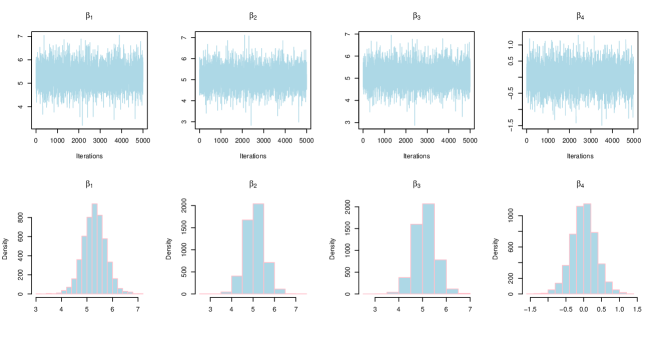
Figure 2: Trace plots and histograms of Simulation 3 using NCG₂.

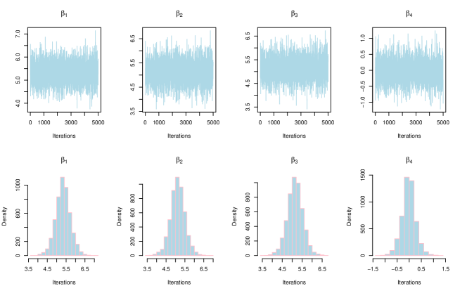
Figure 3: Trace plots and histograms of Simulation 3 using NCG₁₀.

6 A real data example

In this section, we compare the performance of the eight methods in Section 5, NCG₂, NCG₁₀, MCP, SCAD, Enet, Horseshoe, Lasso, aLasso, on the prostate cancer data (Stamey et al., 1989). This data set was used for illustration in previous studies (see, Zou, 2006; Park and Casella, 2008; Mallick and Yi, 2014), where the dependent variable is the logarithm of prostate-specific antigen and the number of covariates are eight clinical measures donated by lcavol = the logarithm of cancer volume, lweight = the logarithm of prostate weight, age, lbph = the logarithm of the amount of benign prostatic hyperplasia, svi = seminal vesicle invasion, lcp = the logarithm of capsular penetration, gleason = the Gleason score, and pgg45 = the percentage Gleason score 4 or 5. We add twelve more predictor noise standard normal random variables, $x_{9},\cdots,x_{20}$. To analyze the data, we follow the methods in (Zou and Hastie, 2005) and (Mallick and Yi, 2014) by dividing it into a training set with 67 observations and a testing set with 30 observations. The results are summarized in Table 8. We can see clearly, that the proposed method performs better than the other methods.

Table 8: Results for the real data.

Methods	MSE (sd)	FPR (sd)
NCG2	18.5125 (0.3134)	0.1200 (0.4798)
NCG10	18.4303 (0.2142)	0.0600 (0.3136)
MCP	19.4068 (0.6941)	0.1800 (0.3881)
SCAD	19.4802 (0.6962)	0.9400 (0.2399)
Enet	20.6716 (0.7222)	0.3400 (0.4785)
Horseshoe	18.7082 (0.2732)	0.0600 (0.3136)
Lasso	18.7504 (0.4828)	1.0000 (0.0000)
aLasso	19.2235 (0.8163)	0.4600 (0.5035)

7 Concluding Remarks

In this paper, we have studied the properties of the normal prior with a compound gamma scale mixture. Then, we proposed a Gibbs sampler and a Variational Bayes method to study the model predictions. Additionally, we incorporated the latter two methods to an EM method to evaluate the corresponding model hyperparameters. Furthermore, we studied posterior consistency of our model using two different sets of conditions for $p_{n}=o(n)$ and $p_{n}\gg n$. Finally, we illustrated our model using simulated and real data examples.

8 Appendix

Proof of Proposition 1..

The proof can be trivially seen using a simple change of variable of integration through $z_{i}\rightarrow x^{(-1)^{i+1}}z^{(-1)^{i}}$

$$\begin{split}\pi(x)&=\int_{0}^{\infty}\ldots\int_{0}^{\infty}\exp\{-z_{2}\}z_{2}^{c_{1}-1}\left[\prod_{i=2}^{M-1}\exp\left\{-\left(\frac{z_{i+1}}{z_{i}}\right)^{(-1)^{i+1}}\right\}\left(\frac{z_{i+1}}{z_{i}}\right)^{(-1)^{i+1}c_{i}-1}\frac{1}{z_{i}}\right]\\ &\qquad\qquad\qquad\qquad\qquad\times\exp\left\{-\phi\left(\frac{z_{1}}{z_{N}}\right)^{(-1)^{N+1}}\right\}\left(\frac{z_{1}}{z_{N}}\right)^{(-1)^{N+1}c_{N}-1}\frac{\phi^{c_{N}}}{z_{N}}d{z}_{2}\ldots d{z}_{N}\\ &=\int_{0}^{\infty}\ldots\int_{0}^{\infty}\mathcal{G}(z_{2},c_{1},1)\frac{\mathcal{IG}(z_{3}/z_{3},c_{2},1)}{z_{2}}\frac{\mathcal{G}(z_{3}/z_{4},c_{3},1)}{z_{3}}\\ &\qquad\qquad\qquad\qquad\qquad\qquad\qquad\qquad\qquad\qquad\qquad\ldots\times\frac{\mathcal{AG}(z_{1}/z_{N},N,c_{N},\phi)}{z_{N}}d{z}_{2}\ldots d{z}_{N}\end{split}$$ (21)

∎

Proof of Theorem 1..

Lemma 1.

If ${c_{1}}_{n}\rightarrow 0$ and $c_{2}\in(1,\infty)$ as $n\rightarrow\infty$, then $\frac{\Gamma({c_{1}}_{n}+c_{2})}{\Gamma({c_{1}}_{n})\Gamma(c_{2})}\asymp{c_{1}}_{n}$.

Proof.

The details can be found in (Bai and Ghosh, 2018). ∎

By the symmetry of the probability for a single density function given by (15)

$$\begin{split}1-\int_{-k_{n}}^{k_{n}}f(x)dx&=2\int_{k_{n}}^{\infty}f(x)dx\\ &\leq 2\int_{0}^{\infty}\ldots\int_{0}^{\infty}\left[\frac{\exp\left\{-k_{n}^{2}/{2z_{1}}\right\}}{\sqrt{2\pi z_{1}}}\prod_{i=1}^{N}\frac{{z}_{i+1}^{c_{i}}}{\Gamma(c_{i})}{z}_{i}^{c_{i}-1}\exp\left\{-{z}_{i}{z}_{i+1}\right\}\right]d{z}_{1}\ldots d{z}_{N}\\ &\leq 2c_{1_{n}}\int_{0}^{\infty}\ldots\int_{0}^{\infty}\int_{0}^{\infty}\bigg{[}\frac{\exp\left\{-k_{n}^{2}/{2z_{1}}\right\}}{\sqrt{2\pi z_{1}}}\frac{{z}_{1}^{c_{1}-1}{z}_{3}^{c_{2}}}{({z}_{1}+{z}_{3})^{c_{1}+1}}\\ &\qquad\qquad\qquad\qquad\qquad\qquad\times\prod_{i=3}^{N}\frac{{z}_{i+1}^{c_{i}}}{\Gamma(c_{i})}{z}_{i}^{c_{i}-1}\exp\left\{-{z}_{i}{z}_{i+1}\right\}\bigg{]}d{z}_{1}d{z}_{3}\ldots d{z}_{N}\\ &\leq 2c_{1_{n}}\int_{0}^{\infty}\ldots\int_{0}^{\infty}\int_{0}^{\infty}\bigg{[}\frac{\exp\left\{-k_{n}^{2}u/2\right\}}{({z}_{3}u+1)^{c_{1}+1}}\\ &\qquad\qquad\qquad\qquad\qquad\qquad\times{z}_{3}^{c_{2}}\prod_{i=3}^{N}\frac{{z}_{i+1}^{c_{i}}}{\Gamma(c_{i})}{z}_{i}^{c_{i}-1}\exp\left\{-{z}_{i}{z}_{i+1}\right\}\bigg{]}dud{z}_{3}\ldots d{z}_{N}\\ &\leq\frac{8c_{1_{n}}}{k_{n}^{2}}\int_{0}^{\infty}\ldots\int_{0}^{\infty}\bigg{[}{z}_{3}^{c_{2}}\prod_{i=3}^{N}\frac{{z}_{i+1}^{c_{i}}}{\Gamma(c_{i})}{z}_{i}^{c_{i}-1}\exp\left\{-{z}_{i}{z}_{i+1}\right\}\bigg{]}d{z}_{3}\ldots d{z}_{N}\\ &=\frac{8c_{1_{n}}}{k_{n}^{2}}\frac{\Gamma[c_{2}+c_{3}]}{\Gamma(c_{3})}\int_{0}^{\infty}\ldots\int_{0}^{\infty}\bigg{[}z_{4}^{-c_{2}}\prod_{i=4}^{N}\frac{{z}_{i+1}^{c_{i}}}{\Gamma(c_{i})}{z}_{i}^{c_{i}-1}\exp\left\{-{z}_{i}{z}_{i+1}\right\}\bigg{]}d{z}_{4}\ldots d{z}_{N}\\ \end{split}$$ (22)

where we have used a change of variable $u=1/z_{1}$ in the third inequality. By repeating the last step, we get

$$\begin{split}1-\int_{-k_{n}}^{k_{n}}f(x)dx\leq\frac{8c_{1_{n}}\phi^{(-1)^{N}c_{2}}}{k_{n}^{2}}\prod_{i=3}^{N}\frac{\Gamma[(-1)^{i+1}c_{2}+c_{i}]}{\Gamma[c_{i}]}\\ \end{split}$$ (23)

where we have used the concentration inequality, $\Pr(|X|>k_{n})\leq 2e^{-k_{n}^{2}/{2z_{1}}}$, and the assumption $b\in(1,\infty)$. For the second condition we have

$$\begin{split}\inf_{x\in[-E_{n},E_{n}]}f(x)&\gtrsim c_{1_{n}}\int_{0}^{\infty}\ldots\int_{0}^{\infty}\int_{0}^{\infty}\bigg{[}\frac{{z}_{1}^{c_{1}-3/2}{z}_{3}^{c_{2}}\exp\left\{-{x^{2}}/{\left(2z_{1}\right)}\right\}}{({z}_{1}+{z}_{3})^{c_{1}+c_{2}}}\\ &\qquad\qquad\qquad\qquad\times\prod_{i=3}^{N}\frac{{z}_{i+1}^{c_{i}}}{\Gamma(c_{i})}{z}_{i}^{c_{i}-1}\exp\left\{-{z}_{i}{z}_{i+1}\right\}\bigg{]}d{z}_{1}d{z}_{3}\ldots d{z}_{N}\\ &\geq c_{1_{n}}(x^{2})^{c_{1}-\frac{1}{2}}\int_{0}^{\infty}\ldots\int_{0}^{\infty}\int_{1}^{2}\biggr{[}\prod_{i=3}^{N}\frac{{z}_{i+1}^{c_{i}}}{\Gamma(c_{i})}{z}_{i}^{c_{i}-1}\exp\left\{-{z}_{i}{z}_{i+1}\right\}\\ &\times\exp\left(-\zeta\right)\left(\frac{\zeta}{x^{2}+2\zeta{z}_{3}}\right)^{c_{2}-1/2}\left(\frac{1}{x^{2}+2\zeta{z}_{3}}\right)^{c_{1}+1/2}\biggr{]}d\zeta d{z}_{3}\ldots d{z}_{N}\\ &\gtrsim c_{1_{n}}(x^{2})^{c_{1}-\frac{1}{2}}\int_{0}^{\infty}\ldots\int_{0}^{\infty}\int_{1}^{2}\biggr{[}z_{3}^{c_{2}}\prod_{i=3}^{N}\frac{{z}_{i+1}^{c_{i}}}{\Gamma(c_{i})}{z}_{i}^{c_{i}-1}\exp\left\{-{z}_{i}{z}_{i+1}\right\}\\ &\qquad\qquad\times\left(\frac{1}{x^{2}+2{z}_{3}}\right)^{c_{2}-1/2}\left(\frac{1}{x^{2}+4{z}_{3}}\right)^{c_{1}+1/2}\biggr{]}d{z}_{3}d{z}_{4}\ldots d{z}_{N}\\ &\gtrsim\frac{c_{1_{n}}}{\left(x^{2}\right)^{c_{2}+1/2}}\int_{0}^{\infty}\ldots\int_{0}^{\infty}\biggr{[}z_{4}^{c_{3}}\prod_{i=4}^{N}\frac{{z}_{i+1}^{c_{i}}}{\Gamma(c_{i})}{z}_{i}^{c_{i}-1}\exp\left\{-{z}_{i}{z}_{i+1}\right\}\biggr{]}d{z}_{4}\ldots d{z}_{N}\\ \end{split}$$ (24)

using ${z}_{i}^{c_{i}+c_{i+1}-1}\geq 1,\forall z_{i}\in[1,2]$ and where we have used $\zeta=\frac{x^{2}}{2{z}_{1}}$ in the second inequality. Using assumptions $\log E_{n}=O(\log p_{n})$ and $c_{1_{n}}\lesssim k_{n}^{2}p_{n}^{-(1+u)}$ for $u>0$ then

$$-\log\left(\inf_{x\in[-E_{n},E_{n}]}f(x)\right)\lesssim\log p_{n}$$ (25)

∎

Proof of Theorem 3.

Using equation $(A3)$ in (Armagan et al., 2013)

$$\begin{split}\Pi_{n}&\left(\beta_{n}:\parallel\beta_{n}-\beta_{n}^{0}\parallel<\frac{\Delta}{n^{\rho/2}}\right)\geq\left\{1-\frac{p_{n}n^{\rho}\mathbb{E}(\beta^{2}_{n_{j}})}{\Delta^{2}}\right\}\\ &\prod_{j\in\Theta_{n}}\left\{\Pi_{n}\left(\beta_{n_{j}}:|\beta_{n_{j}}-\beta^{0}_{n_{j}}|<\frac{\Delta}{\sqrt{p_{n}}n^{\rho/2}}\right)\right\}\\ \end{split}$$ (26)

Using $\mathbb{E}(\beta^{2})=\frac{\sigma^{2}c_{1}c_{3}c_{5}\ldots c_{N}\phi^{(-1)^{N}}}{(c_{2}-1)(c_{4}-1)\ldots(c_{N-1}-1)}$ and the second part of the proof of Theorem 1, then

$$\begin{split}\Pi_{n}&\left(\beta_{n}:\parallel\beta_{n}-\beta_{n}^{0}\parallel<\frac{\Delta}{n^{\rho/2}}\right)\geq\left\{1-\frac{p_{n}n^{\rho}}{\Delta^{2}}\frac{\sigma^{2}c_{1}c_{3}c_{5}\ldots c_{N}\phi^{(-1)^{N}}}{(c_{2}-1)(c_{4}-1)\ldots(c_{N-1}-1)}\right\}\\ &\times\left[\frac{2\Delta c_{1_{n}}}{\sqrt{p_{n}}n^{\rho/2}}\left\{\frac{\sup_{j\in\mathcal{A}_{n}}(\beta^{0}_{nj})^{2}}{\phi_{n}}+\frac{\Delta^{2}}{p_{n}n^{\rho}\phi_{n}}\right\}^{-c_{2}-1/2}\right]^{s_{n}}\\ \end{split}$$ (27)

∎

letting $\phi_{n}=C/(p_{n}n^{\rho}\log n)$ for some $C>0$ and taking the negative log of both side, we can easily see that $\Pi_{n}\left(\beta_{n}:\parallel\beta_{n}-\beta_{n}^{0}\parallel<\frac{\Delta}{n^{\rho/2}}\right)<dn,\forall d>0$ which completes the prove.

References

- Akaike (1973) Akaike, H. (1973). Information theory and an extension of maximum likelihood principle. In Second International Symposium on Information Theory, B. N. Petrov and F. Csaki (eds), Budapest: Akademiai Kiado.
- Alhamzawi and Ali (2018) Alhamzawi, R. and H. T. M. Ali (2018). Bayesian quantile regression for ordinal longitudinal data. Journal of Applied Statistics 45(5), 815–828.
- Armagan et al. (2011) Armagan, A., M. Clyde, and D. Dunson (2011). Generalized beta mixtures of gaussians. Advances in neural information processing systems 24.
- Armagan et al. (2013) Armagan, A., D. B. Dunson, J. Lee, W. U. Bajwa, and N. Strawn (2013). Posterior consistency in linear models under shrinkage priors. Biometrika 100(4), 1011–1018.
- Bai and Ghosh (2018) Bai, R. and M. Ghosh (2018). On the beta prime prior for scale parameters in high-dimensional bayesian regression models. arXiv preprint arXiv:1807.06539.
- Bishop and Tipping (2000) Bishop, C. M. and M. E. Tipping (2000). Variational relevance vector machines. In Proceedings of the 16th Conference on Uncertainty in Artificial Intelligence, pp. 46–53. Morgan Kaufmann.
- Carvalho et al. (2010) Carvalho, C. M., N. G. Polson, and J. G. Scott (2010). The horseshoe estimator for sparse signals. Biometrika 97(2), 465–480.
- Castillo et al. (2015) Castillo, I., J. Schmidt-Hieber, and A. Van der Vaart (2015). Bayesian linear regression with sparse priors. The Annals of Statistics 43(5), 1986–2018.
- Fan and Li (2001) Fan, J. and R. Li (2001). Variable selection via nonconcave penalized likelihood and its oracle properties. Journal of the American statistical Association 96(456), 1348–1360.
- Frank and Friedman (1993) Frank, L. E. and J. H. Friedman (1993). A statistical view of some chemometrics regression tools. Technometrics 35(2), 109–135.
- Gefang (2014) Gefang, D. (2014). Bayesian doubly adaptive elastic-net lasso for var shrinkage. International Journal of Forecasting 30(1), 1–11.
- Huang et al. (2009) Huang, J., S. Ma, H. Xie, and C.-H. Zhang (2009). A group bridge approach for variable selection. Biometrika 96(2), 339–355.
- Johnson and Rossell (2012) Johnson, V. E. and D. Rossell (2012). Bayesian model selection in high-dimensional settings. Journal of the American Statistical Association 107(498), 649–660.
- Jordan et al. (1999) Jordan, M. I., Z. Ghahramani, T. S. Jaakkola, and L. K. Saul (1999). An introduction to variational methods for graphical models. Machine learning 37(2), 183–233.
- Kyung et al. (2010) Kyung, M., J. Gill, M. Ghosh, G. Casella, et al. (2010). Penalized regression, standard errors, and Bayesian lassos. Bayesian Analysis 5(2), 369–411.
- Li et al. (2010) Li, Q., N. Lin, et al. (2010). The Bayesian elastic net. Bayesian Analysis 5(1), 151–170.
- Mallick et al. (2021) Mallick, H., R. Alhamzawi, E. Paul, and V. Svetnik (2021). The reciprocal Bayesian lasso. Statistics in medicine 40(22), 4830–4849.
- Mallick and Yi (2014) Mallick, H. and N. Yi (2014). A new Bayesian lasso. Statistics and its interface 7(4), 571.
- Mallows (1973) Mallows, C. L. (1973). Some comments on c p. Technometrics 15(4), 661–675.
- Park and Casella (2008) Park, T. and G. Casella (2008). The Bayesian Lasso. Journal of the American Statistical Association 103, 681–686.
- Pérez et al. (2017) Pérez, M.-E., L. R. Pericchi, and I. C. Ramírez (2017). The scaled beta2 distribution as a robust prior for scales. Bayesian Analysis 12(3), 615–637.
- Polson et al. (2014) Polson, N. G., J. G. Scott, and J. Windle (2014). The bayesian bridge. Journal of the Royal Statistical Society: Series B (Statistical Methodology) 76(4), 713–733.
- Ročková and George (2018) Ročková, V. and E. I. George (2018). The spike-and-slab lasso. Journal of the American Statistical Association 113(521), 431–444.
- Schwarz et al. (1978) Schwarz, G. et al. (1978). Estimating the dimension of a model. The annals of statistics 6(2), 461–464.
- Shin et al. (2018) Shin, M., A. Bhattacharya, and V. E. Johnson (2018). Scalable Bayesian variable selection using nonlocal prior densities in ultrahigh-dimensional settings. Statistica Sinica 28(2), 1053.
- Song and Liang (2015) Song, Q. and F. Liang (2015). High-dimensional variable selection with reciprocal -regularization. Journal of the American Statistical Association 110(512), 1607–1620.
- Song and Liang (2017) Song, Q. and F. Liang (2017). Nearly optimal bayesian shrinkage for high dimensional regression. arXiv preprint arXiv:1712.08964.
- Spiegelhalter et al. (2002) Spiegelhalter, D. J., N. G. Best, B. P. Carlin, and A. Van Der Linde (2002). Bayesian measures of model complexity and fit. Journal of the royal statistical society: Series b (statistical methodology) 64(4), 583–639.
- Stamey et al. (1989) Stamey, T. A., J. N. Kabalin, J. E. McNeal, I. M. Johnstone, F. Freiha, E. A. Redwine, and N. Yang (1989). Prostate specific antigen in the diagnosis and treatment of adenocarcinoma of the prostate. ii. radical prostatectomy treated patients. The Journal of urology 141(5), 1076–1083.
- Tibshirani (1996) Tibshirani, R. (1996). Regression shrinkage and selection via the Lasso. Journal of the Royal Statistical Society, Series B 58, 267–288.
- Wei and Tanner (1990) Wei, G. C. and M. A. Tanner (1990). A monte carlo implementation of the em algorithm and the poor man’s data augmentation algorithms. Journal of the American statistical Association 85(411), 699–704.
- Xu and Ghosh (2015) Xu, X. and M. Ghosh (2015). Bayesian variable selection and estimation for group lasso. Bayesian Analysis 10(4), 909–936.
- Yuan and Lin (2005) Yuan, M. and Y. Lin (2005). Model selection and estimation in regression with grouped variables. Journal of the Royal Statistical Society, Series B 68, 49–67.
- Zhang (2010) Zhang, C.-H. (2010). Nearly unbiased variable selection under minimax concave penalty. The Annals of statistics 38(2), 894–942.
- Zou (2006) Zou, H. (2006). The adaptive lasso and its oracle properties. Journal of the American statistical association 101(476), 1418–1429.
- Zou and Hastie (2005) Zou, H. and T. Hastie (2005). Regularization and variable selection via the elastic net. Journal of the Royal Statistical Society, Series B 67, 301–320.
- Zou and Zhang (2009) Zou, H. and H. H. Zhang (2009). On the adaptive elastic-net with a diverging number of parameters. The Annals of Statistics 37, 1733–1751.