Towards a Multimodal Charging Network: Joint Planning of Charging Stations and Battery Swapping Stations for Electrified Ride-Hailing Fleets

Abstract

This paper considers a multimodal charging network in which charging stations and battery swapping stations are jointly built to support the electrified ride-hailing fleet in a synergistic manner. Our central thesis is predicated on the observation that charging stations are cost-effective, making them ideal for scaling up electric vehicles in ride-hailing fleets in the beginning, while battery swapping stations offer quick turnaround and can be deployed in tandem with charging stations to improve fleet utilization and reduce operational costs for the ride-hailing platform. To fulfill this vision, we consider a ride-hailing platform that expands the multimodal charging network with a multi-stage investment budget and operates a ride-hailing fleet to maximize its profit. A multi-stage network expansion model is proposed to characterize the coupled planning and operational decisions, which captures demand elasticity, passenger waiting time, charging and swapping waiting times, as well as their dependence on fleet status and charging infrastructure. The overall problem is formulated as a nonconvex program. Instead of pursuing the globally optimal solution, we establish a theoretical upper bound through relaxation, reformulation, and decomposition so that the global optimality of solutions to the nonconvex problem is verifiable. In the case study for Manhattan, we find that a swapping-only strategy slows the electrification of ride-hailing fleets and results in a longer pay-back period for the investment, especially under a limited budget. A charging-only strategy yields a lower total profit due to its inherent bottleneck. In contrast, joint planning can combine the benefit of both facilities as they can complement each other and play different roles during the expansion of a charging infrastructure network. The platform prefers to build charging stations at the early stage to quickly electrify the fleet and then deploys swapping stations to enhance fleet utilization, highlighting the synergistic value in the proposed multimodal charging network.

1 Introduction

The electrification of transportation is essential for establishing a green and sustainable mobility future. In recent years, governments across the globe have committed to supporting the adoption of electric vehicles (EVs) through a suite of regulations and subsidies. Among all types of vehicles, it is widely accepted that commercial fleets (e.g., ride-hailing cars) contribute to higher annual mileage and thus represent a prospective growth area for transport electrification and pollution reduction. Currently, Uber provides approximately 21 million rides per day in over 10,000 cities [1], and Didi’s global daily trips can even exceed 50 million [2]. However, the vast majority of these rides are delivered by fossil fuel vehicles. EVs merely account for less than 5% of miles driven by Uber drivers in Europe [3], and less than 0.5% in the US [4], whereas the potential environmental benefits of electrifying ride-hailing fleets could be three times higher than those of electrifying private cars [5]. To unlock this enormous potential, California regulators have passed a legislation requiring transportation network companies to convert from petroleum to electric vehicles by 2030 [6]. In response, both Uber and Lyft have pledged to offer zero-emission mobility-on-demand services by the end of the decade [7, 8].

However, charging infrastructure remains a persistent barrier that hinders the electrification of ride-hailing fleets in the long term. Different from private cars, commercial fleets need to run on the road as long as possible to accrue profits, while most ride-hailing EV drivers need to top up the batteries once or twice every day due to the limited battery range [9]. Typically, EV charging takes a longer time than filling the gas tank, and this charging downtime could result in a significant opportunity cost [10], making EVs less appealing for ride-hailing use. As per [11], charging time comprises 72-75% of the total downtime spent on charging trips. This indicates that charging time, as opposed to travel time or waiting time, is the dominant bottleneck for EV charging, even with a dense charging station network. To address this challenge, manufacturers are massively investing in fast charging technologies, which can offer battery top-up at a much faster speed: Tesla’s supercharger can recharge up to 200 miles in 15 minutes [12]. However, fast charging typically relies on high voltage and draws significant power from the grid. As a result, it is impractical to deploy a large number of fast chargers in crowded urban locations, as doing so could cause considerable voltage drop and instability in the aging power distribution network, which is already under stress and can be prohibitively expensive to rebuild. For this reason, plug-in charging stations presents an inherent bottleneck for the ride-hailing industry: regardless of the density of the charging network, there is always a significant downtime for the commercial fleet due to the limited charging speed that can be maximally supported by the capacity of existing power distribution networks in large metropolitan areas. This leads to low fleet utilization and high operational costs for the ride-hailing platform.

Battery swapping is an alternative method for recharging depleted EVs, where an empty battery is replaced with a fully charged one in a few minutes. There was a heated debate over plug-in charging and battery swapping, after which many western countries predominantly invested in charging stations instead of battery swapping stations. One primary reason for this preference is the lack of standardized batteries among EV manufacturers. In contrast, China takes a more impartial stance, encouraging both plug-in charging and battery swapping technologies. This policy is based on the belief that, standardizing batteries is more feasible for commercial vehicles than for privately-owned EVs. In recent years, governments are pushing electrification among taxi fleets, which naturally come with a unified battery model (see Shenzhen [13] for an example). In the private sector, ride-hailing platforms have actively collaborated with automobile manufacturers to produce affordable EVs tailored for ride-hailing services. Notable examples include the battery-swappable Cao Cao 60 [14], a joint effort between Caocao Mobility and Geely, and the D1 [15], co-developed by Didi and BYD. Uber is also working with automakers to create custom-made EVs for ride-hailing and delivery applications [16]. Large-scale deployment of these customized EVs can naturally address the compatibility issue, making battery swapping a viable solution. In addition, it is envisioned that future mobility-on-demand systems will be driven by electric and autonomous vehicles that are under centralized control of the platform. In fact, both Uber and Didi have announced their plans to offer services using robotaxis [17][18]. This important trend further justifies a unified battery standard and the feasibility of battery swapping. The advantages of battery swapping can be tremendous for electric ride-hailing fleets: it enables faster recharge than the fastest charger, which can substantially reduce charging downtime, improve fleet utilization, and thereby enhance business sustainability. In this regard, battery swapping is a competitive solution for large commercial fleets and is attracting increasing attention in the industry recently. For instance, BP has partnered with Chinese battery swapping specialist Aulton to offer services for taxis, ride-hailing vehicles, and other passenger cars [19]. GCL-ET aims to recharge 10,000 electric taxis and ride-hailing cars by building a battery swapping network with a service radius of 3 kilometers in Guangzhou, China by the end of 2025, with the first batch of 12 battery swapping stations put into operation lately [20]. San Francisco-based startup Ample provides battery swapping services for Uber and other commercial EVs using modular power packs. They estimate that a ride-hailing driver only needs to spend 3.6 hours per week charging their EV using battery swapping, which is 86% less time than using fast charging [21]. Nevertheless, we must recognize that scaling a battery swapping network takes longer due to its much higher deployment costs.

To combine the advantages of plug-in charging and battery swapping, we propose a multimodal charging network in which charging stations and battery swapping stations are jointly built to support the electrified ride-hailing fleet. Our central thesis is predicated on the observation that charging stations are cost-effective, making them ideally suitable for scaling up EV adoption in the beginning, while battery swapping stations offer quicker turnaround and can be deployed in tandem with charging stations to improve fleet utilization and reduce operational costs. To realize this vision, we consider a multi-stage infrastructure planning problem in which a profit-maximizing platform jointly deploys charging and battery swapping stations with a limited budget and simultaneously operates a ride-hailing fleet comprised of both EVs and gasoline vehicles to serve customers over a transportation network. A multi-stage charging network expansion model is proposed to decide when and where to deploy each type of charging facility, along with the ride-hailing operational decisions including pricing strategies, fleet management strategies, and charging mode choices. The key contributions of this paper are summarized as follows:

1. This paper examines the benefits of a multimodal charging network consisting of both charging stations and battery swapping stations, with an emphasis on exploring their synergistic benefits. Despite extensive research on charging infrastructure planning, the complementary effects between these two facilities have been overlooked in the existing literature. To the best of our knowledge, this paper makes the first attempt to investigate the multimodal charging network by considering the joint deployment of charging stations and battery swapping stations.

2. We propose a multi-stage charging network expansion model to depict the coupled infrastructure planning and operational decisions in a ride-hailing network. This model integrates fundamental elements, including demand elasticity, passenger waiting time, charging and swapping waiting times, and their dependence on fleet status and charging infrastructure. The stationary charging demand is analytically derived given passenger demand patterns and vehicle flows, and the congestion at different facilities is characterized by queuing-theoretic models. The network expansion problem is formulated as a nonconvex optimization problem spanning multiple stages.

3. We establish a tight upper bound for the joint deployment problem despite its nonconvexity. Through model relaxation and transformation, we develop a reformulation that is decomposable in both spatial and temporal dimensions, enabling us to solve the reformulation by separately addressing multiple small-scale subproblems. We further leverage the special problem structure to show that each nonconvex subproblem can be optimally solved. Solutions to subproblems offer a theoretical upper bound that can be used to evaluate the global optimality of solutions to the original problem.

4. We verify the effectiveness of joint deployment with realistic case studies for Manhattan and provide insights into infrastructure planning. We find that a swapping-only strategy results in slower fleet electrification and a longer pay-back period for the investment, while a charging-only strategy leads to longer fleet downtime and a lower profit. In comparison, joint planning combines their benefits and outperforms solely deploying one of them in terms of profit maximization. The two facilities complement each other and play different roles during the expansion of an infrastructure network.

2 Literature Review

2.1 Modeling Electric Ride-Hailing Markets

In ride-hailing markets, EV fleets differ from the gasoline-powered one in that EV charging would intermittently interrupt services and result in lengthy downtime, which impacts the platform’s operation and necessitates special consideration in the formulation of mathematical models, the design of operational strategies, as well as the formation of regulatory policies.

One of the key topics for electric ride-hailing markets is the charging and operational strategies for EVs. Many studies focus on capturing the distinct driving patterns of ride-hailing EV drivers. For instance, Ke et al. [22] modeled drivers’ behavior in a ride-sourcing market with EVs and gasoline vehicles, developed a time-expanded network to sketch out drivers’ working and recharging schedules, and found that passengers, drivers, and the platform are all worse off when the charging price increases. Qin et al. [23] used a multi-state model to identify two distinct driving patterns for ride-hailing EVs, which outline when, for how long, and under what state of charge a driver will decide to recharge an EV. Alam [24] emulated the daily trip patterns of ride-sourcing EVs using an optimization-based method and investigated the induced charging demand using agent-based simulation. Besides, a growing body of literature highlights the operations of electric ride-hailing markets. Shi et al. [25] formulated a dynamic vehicle routing problem (VRP) to capture the operations of a ride-hailing EV fleet and solved the problem using reinforcement learning. Kullman et al. [26] also employed deep reinforcement learning to develop operational polices for ride-hailing EVs, which includes vehicle assignment, charging, and repositioning decisions. Pricing strategies are considered in [27], where Hong and Liu examined the optimal price and wage of green ride services while taking into account the opportunity cost of EV drivers as well as passengers’ willingness to pay for eco-friendly trips. Ding et al. [28] considered the integration of ride-hailing and vehicle-to-grid (V2G) services and developed a game-theoretic framework to characterize the market equilibrium. Cai et al. [29] investigated the operations of integrated ride-sourcing and EV charging services in a nested two-sided market framework. Furthermore, related research is expanded into shared autonomous electric vehicles (SAEVs) [30][31][32][33]. Among others, Turan et al. [31] considered pricing, routing, and charging strategies. Yi and Smart [32] focused on joint dispatching and charging management. Al-Kanj et al. [33] used approximate dynamic programming to develop high-quality pricing, dispatching, repositioning, charging, and fleet sizing strategies for the operations of an SAEV fleet.

Another important topic is on policies that promote the electrification of ride-hailing industry. Different policy options have been explored in the literature, with a primary focus on pricing incentives that includes subsidy for EV purchases, incentive schemes for EV rental, and financial support to infrastructure supply [4][10][34][35][36][37]. Particularly, Liu et al. [10] examined the market response and electrification levels under three different regulatory policies, including annual permit fees, differential trip-based fees, and differential commission caps. They indicated that the last policy is the most cost-efficient and can simultaneously benefit drivers and passengers. Slowik et al. [34] also found that well-designed taxes and fee structures can make EVs the most economically attractive technology for ride-hailing fleets. As per [37], governments should shift the target of current subsidies to the most intensively-used vehicles and the people most in need of financial support, for instance, ride-hailing drivers. And ensuring access to overnight charging is another crucial step to dismantling barriers to vehicle electrification. However, Mo et al. [35] showed that given a limited budget, governments should subsidize charging infrastructure before supporting EV purchase. We comment that all aforementioned works focus on the operational strategies and/or public policies for electric ride-hailing fleets, while the planning of charging infrastructure for the ride-hailing network is not explicitly considered.

2.2 Infrastructure Planning for EV fleets

Charging infrastructure is a crucial component in a green and sustainable mobility ecosystem. In the existing literature, the planning strategies of EV infrastructure, including both charging stations and battery swapping stations, have been extensively examined (see [38] for a comprehensive summary). Unlike private EVs that typically charge at home, commercial EV fleets have significantly higher mileage and rely heavily on public charging stations, requiring extra infrastructure planning considerations. In light of this, we review relevant studies that focus on infrastructure planning for commercial EV fleets, such as those in electric ride-hailing markets.

A recurrent topic in the literature is planning charging stations for EV fleets that offer mobility-on-demand services over the transportation network. Brandstätter et al. [39] studied optimal locations of charging stations for a car-sharing EV fleet considering demand stochasticity. Roni et al. [11] tackled charging station allocation and car-sharing EV assignment in a joint optimization framework and confirmed that charging time is a dominant component of the total fleet downtime. Ma and Xie [40] also jointly considered infrastructure planning and vehicle assignment problem for ride-hailing EVs and formulated a bi-level problem to minimize the charging operation time. Alam and Guo [41] took drivers’ value of time into account in planning charging stations for ride-hailing EVs. Bauer et al. [42] adopted agent-based simulation to analyze charging infrastructure for electrified ride-hailing fleets and suggested that the cost of charging infrastructure accounts for a small fraction of the total cost of an electric ride-hailing trip. Following Lyft’s announcement to reach 100% EVs, Jenn [43] examined the infrastructure deployment necessary to meet charging demand from fully-electrified fleets in California and found that a shift from daytime charging to overnight charging can significantly reduce costs.

The planning of battery swapping stations also attracts a lot of research focus. Mak et al. [44] developed a robust optimization framework to deploy battery swapping facilities and investigated how battery standardization and technology advancements will impact the optimal deployment strategy. Targeted at refueling electric taxicabs, Wang et al. [45] jointly tackled the deployment of battery swapping stations and charging scheduling of EV fleets and designed a planning scheme to decrease in-station queuing time and improve quality of service of the taxicab fleet. Infante et al. [46] considered stochastic charging demand and formulated a two-stage optimization with recourse, where battery swapping stations are deployed in the planning stage and the infrastructure network is coordinated in the operation stage. Further, Yang et al. [47] proposed a data-driven approach to deploying and operating battery swapping stations with centralized management. Moon et al. [48] examined the locating problem of battery swapping stations in a passenger traffic network to achieve the seamless operation of electric buses.

Despite a large volume of literature on charging infrastructure planning for electric ride-hailing fleets, all existing works focus only on one type of charging infrastructure (either charging stations or battery swapping stations). This paper distinguishes from all previous studies in that we consider a multimodal charging network where charging stations and battery swapping stations are jointly deployed to overcome their respective limitations and maximize their complementary effects. To the best of our knowledge, this consideration has not been studied in the literature before.

3 Mathematical Formulation

We consider a platform that offers on-demand ride-hailing services over a transportation network using a mixed fleet of EVs and gasoline vehicles. To support EV charging, the platform collaborates with charging infrastructure providers to devise a long-term infrastructure investment that spans $T$ stages (e.g, each stage corresponds to 2 year) subject to a limited budget. At each stage, the platform determines how many charging stations and/or battery swapping stations to build, where to deploy the charging infrastructure, and how to operate the ride-hailing fleet under the existing infrastructure network. Overall, the platform makes both planning and operational decisions to maximize its cumulative profit over an infinite operation horizon. Note that infrastructure planning decisions are typically made on a timescale of years, whereas the time-varying travel demand would influence the platform’s operational decisions and thus market outcomes on a much shorter timescale, ranging from minutes to hours. Jointly considering decision-making on these two different timescales is difficult, as it would lead to a very complex problem that is challenging to solve. In this light, the steady-state equilibrium at each stage is assumed to inform infrastructure planning. We emphasize that this is a common assumption in many existing works on ride-hailing markets [10][54][40]. The remainder of this section details a mathematical model for the optimal deployment of a multimodal charging network to support the electrification of ride-hailing fleets.

3.1 Expansion of Charging Networks

Consider a multimodal charging network in a city consisting of $M$ zones. At stage $t$, the platform deploys $x^{c}_{i,t}$ charging stations and $x^{s}_{i,t}$ battery swapping stations in zone $i$. We denote the planning decisions as $x_{t}=[x^{c}_{t},x^{s}_{t}]$, where $x^{c}_{t}=[x^{c}_{1,t},\cdots,x^{c}_{M,t}]$ and $x^{s}_{t}=[x^{s}_{1,t},\cdots,x^{s}_{M,t}]$. For notation convenience, we further denote the accumulated charging infrastructure as $\tilde{x}_{t}=[\tilde{x}^{c}_{t},\tilde{x}^{s}_{t}]$, where $\tilde{x}^{c}_{t}=\sum_{\tau=1}^{t}x^{c}_{\tau}$ and $\tilde{x}^{s}_{t}=\sum_{\tau=1}^{t}x^{s}_{\tau}$ are vectors representing the number of deployed charging and battery swapping stations in each zone up to stage $t$. Let $\tilde{x}_{0}^{c}$ and $\tilde{x}_{0}^{s}$ represent the initial number of charging stations and battery swapping stations, respectively. Clearly, we have the following relation:

$$\tilde{x}_{t}^{c}=\tilde{x}_{t-1}^{c}+x_{t}^{c},\quad t\in\{1,\cdots,T\},$$ (1a)

$$\tilde{x}_{t}^{s}=\tilde{x}_{t-1}^{s}+x_{t}^{s},\quad t\in\{1,\cdots,T\},$$ (1b)

which indicates that the charging infrastructure built at each stage will be available for future use. Let $a_{c}$ and $a_{s}$ denote the per-unit deployment costs for charging and battery swapping facilities, and let $b_{t}$ denote the budget at stage $t$. Assume that all unused budget during stage $t$ can be used in future planning stages, then the planning decisions should satisfy the following budgetary constraint:

$$A^{\top}\tilde{x}_{t}=a_{c}\sum_{i=1}^{M}\tilde{x}_{i,t}^{c}+a_{s}\sum_{i=1}^{M}\tilde{x}_{i,t}^{s}\leq\tilde{b}_{t},$$ (2)

where $A=[a_{c},\ldots,a_{s},\ldots]$, and $\tilde{b}_{t}=\sum_{\tau=1}^{t}b_{\tau}$ is the cumulative budget as of stage $t$.

Given the infrastructure network $\tilde{x}_{t}$ at each stage $t$, the platform determines the operational strategies to maximize its profit. These decisions involve both the supply and demand sides of the ride-hailing market, which are intimately coupled with the planning decisions of charging infrastructure. To characterize this intrinsic correlation, we observe that the impacts of ride-hailing operations can be analyzed in the following sequence: (a) the platform prices its services and dispatches idle vehicles across the transportation network to steer passenger demand; (b) passenger demand induces a flow pattern of EVs, which further generates a spatial distribution of charging demand over the network; (c) the generated charging demand is accommodated by the multimodal charging network, leading to downtime during which vehicles cannot offer ride-hailing services; (d) after completion of charging, EVs resume duty and become available again for ride-hailing services, which affects pickup time and further influences passenger demand. In the rest of this section, we will present the platform’s operational decisions following the aforementioned sequence.

3.2 Managing Passenger Demand

Passengers decides whether to use ride-hailing services or alternative transport modes based on the generalized cost of each ride-hailing trip, which depends on the trip fare and waiting time. At stage $t$, let $p_{i,t}$ be the per-unit-time ride fare for a trip starting from zone $i$, and denote $\tau_{ij}$ as the average duration for a trip from zone $i$ to $j$. In this case, the average total expenditure of a trip from zone $i$ to zone $j$ is $p_{i,t}\tau_{ij}$. We denote $w_{i,t}^{p}$ as the average waiting time before each passenger is picked up. Then the arrival rate of ride-hailing passengers from zone $i$ to zone $j$ can be represented as:

$$\lambda_{ij,t}=\bar{\lambda}_{ij}F_{p}\left(p_{i,t}\tau_{ij}+\alpha w^{p}_{i,t}\right),$$ (3)

where $\bar{\lambda}_{ij}$ is the potential travel demand from zone $i$ to zone $j$, including all passengers regardless of travel modes; $\alpha$ is passengers’ value of time; and $F_{p}(\cdot)$ is a strictly decreasing function that represents the proportion of travelers using ride-hailing services.

In the passenger demand function (3), $p_{i,t}$ is a decision variable, while $w^{p}_{i,t}$ is an endogenous variable that depends on the availability of idle vehicles. This dependence should be quantified through a function that relates the number of idle vehicles to the average pickup time in each zone. For this purpose, we consider a ride-hailing fleet comprised of both EVs and gasoline cars. The platform decides on the composition of the mixed fleet based on their costs and the supply of charging infrastructure and adjusts the spatial distribution of this mixed fleet according to passenger demand in different zones. For simplicity, we assume passengers are indifferent to vehicle types and the platform matches passengers following the first-come-first-serve principle, meaning that each passenger will be immediately matched to the closest idle vehicle, regardless of vehicle types. In this case, the pickup time only depends on the total number of idle vehicles. Denote $N_{i,t}^{ve}$ and $N_{i,t}^{vg}$ as the number of idle EVs and gasoline vehicles in zone $i$ at stage $t$, respectively, and let $N_{t}^{ve}=[N_{1,t}^{ve},\ldots,N_{M,t}^{ve}]$ and $N_{t}^{vg}=[N_{1,t}^{vg},\ldots,N_{M,t}^{vg}]$. The passenger waiting time $w_{i,t}^{p}$, from a ride request being placed to the passenger being picked up, can be captured by the well-established square root law [55][56]:

$$w^{p}_{i,t}=\dfrac{\phi}{\sqrt{N^{ve}_{i,t}+N^{vg}_{i,t}}},$$ (4)

where $\phi$ is a model parameter depending on the geometry of the city. The functional form of (4) is intuitive. As the number of idle vehicles increases subject to a fixed spatial distribution, the distance between a passenger and each of the vehicles will decrease in proportion to the square root of the number of idle vehicles. A rigorous proof for the case of uniform distribution can be found in [56]. Note that the first-come-first-serve matching mechanism is a common assumption in the existing literature on ride-hailing markets [57][58][35][54]. We believe that it does not significantly limit the model’s generality since as the proposed methodology in this paper does not hinge on the square root structure of (4).

Due to the asymmetric passenger demand, the platform further dispatches vehicles from one zone to another to rebalance the fleet. Let $f_{t}=[f_{ij,t}]_{\forall i,j=\{1,\ldots,M\}}$ be the rebalancing flow. In the long run, the vehicle inflow and outflow in each zone should be equal, which leads to the network flow balance constraint:

$$\sum_{j=1}^{M}(\lambda_{ij,t}+f_{ij,t})=\sum_{j=1}^{M}(\lambda_{ji,t}+f_{ji,t}),$$ (5)

where the left-hand side represents the total flow leaving zone $i$, and the right-hand side denotes the total flow entering zone $i$. Note that these delivery and rebalancing trips can be completed by either EVs or gas-powered cars. Since the platform does not prioritize any vehicle type when dispatching the fleet, EVs will be dispatched with a chance of $R_{i,t}=N^{ve}_{i,t}/(N^{ve}_{i,t}+N^{vg}_{i,t})$, and gasoline vehicles with a chance of $1-R_{i,t}$. If the platform adopts EVs in one of the $M$ zones, these EVs will flow into different zones along with the cross-zone trips and end up idling in every zone with a certain probability at equilibrium. To capture this, we enforce the following constraint:

$$N^{ve}_{i,t}>0,\forall i=1,\ldots,M,$$ (6)

which means that EVs will be deployed in each zone of the city. This is a very mild condition because each zone will be the destination of some passengers and thus the probability for each vehicle to visit each zone must be strictly positive in the long run.

3.3 Spatial Distribution of Charging Demand

The stationary distribution of charging demand is defined as the long-run probability that an EV will need to be recharged in one of the $M$ zones. Assuming that each EV will be sent to top up when its state of charge falls below a random threshold with a mean value of $\epsilon$, a certain proportion of EVs will run out of power in each zone in the long run. We further assume that before the EV’s remaining range hits the threshold, the movement of this vehicle over the transportation network is completely governed by random demand and is oblivious to its random threshold. Consequently, the spatial distribution of charging demand follows the equilibrium fleet distribution, which further depends on the EV fleet movement and is inherently affected by the platform’s operational decisions.

Following the idea in [59], we consider the EV fleet movement as a random walk with a certain transition matrix $P$. To derive the transition matrix, we first note that the operating hours of EVs consist of idle trips (waiting for the next passenger), pickup trips (heading to pick up an assigned passenger), delivery trips (transporting passengers to destinations), and rebalancing trips (relocating from one zone to another with empty seats). The first two categories are regarded as intra-zone trips, while the last two types can be either inter-zone or intra-zone trips depending on destinations. In this light, we define $D_{ij,t}$ to capture the average number of EVs that travel from zone $i$ to zone $j$ (either with or without a passenger):

$$D_{ij,t}= N^{ve}_{i,t}+R_{i,t}\sum_{j=1}^{M}\left(\lambda_{ij,t}w^{p}_{i,t}+\lambda_{ii,t}\tau_{ii}+f_{ii,t}\tau_{ii}\right),\quad i=j$$ , (7a)

$$D_{ij,t}= R_{i,t}\left(\lambda_{ij,t}\tau_{ij}+f_{ij,t}\tau_{ij}\right),\quad i\neq j$$ . (7b)

The last three terms in (7a) follow the Little’s law and respectively represent the number of EVs undergoing pickup, delivery, and rebalancing trips. With this information, we can compute the transition matrix $P_{t}$:

$$P_{ij,t}=\dfrac{D_{ij,t}}{\sum_{j=1}^{M}D_{ij,t}},$$ (8)

which captures the probability of an EV departing for zone $j$ given that it is currently in zone $i$. Let $n_{t}=[n_{1,t},\cdots,n_{M,t}]$ be a positive row vector denoting the probability that each EV will stay in each zone at equilibrium. Based on the above analysis, $n_{t}$ further represents the stationary charging demand distribution. Clearly, each element of $n_{t}$ should be positive, and we have $\sum_{i=1}^{M}n_{i,t}=1$. The derivation of $n_{t}$ follows the proposition below:

Proposition 1.

For any $\lambda_{ij,t}>0$ and $N^{ve}_{i,t}>0$, the stationary charging demand distribution $n_{t}$ exists and is uniquely given by

$$n_{t}P_{t}=n_{t}.$$ (9)

Proof.

Since $\lambda_{ij,t}>0$ and $N^{ve}_{i,t}>0$, we know that $D_{ij,t}>0,\forall i,j$ and thus $P_{t}$ is element-wise strictly positive. And every row of $P_{t}$ adds to 1, so it is a row stochastic matrix. According to the Perron–Frobenius theorem [60], $P_{t}$ has an eigenvalue 1 and the corresponding left eigenvector is unique and has all-positive entries. Therefore, solving (9) yields a unique stationary charging demand distribution $n_{t}$. ∎

The strict positivity of $\lambda_{ij,t}$ is a mild assumption as it only requires the platform to provide services for each OD pair. Given the charging demand distribution $n_{t}$, we define $k_{i,t}$ as the arrival rate of charging requests in zone $i$. Then $k_{t}=[k_{1,t},\ldots,k_{M,t}]$ represents the stationary charging demand among different zones. Clearly, $k_{i,t}$ should be proportional to $n_{i,t}$ and thus we have:

$$k_{i,t}=n_{i,t}\sum_{j=1}^{M}k_{j,t}.$$ (10)

The induced charging demand $k_{i,t}$ will be accommodated by charging stations or battery swapping stations in each zone. We will characterize the charging process in the next subsection.

Remark 1.

In practice, EVs can be relocated to a neighboring zone for plug-in charging or battery swapping when local charging facilities are congested. This charging dispatch decision is captured in the proposed charging demand distribution model. Specifically, the platform can adjust the rebalancing flow $f_{t}$ to affect the transition matrix $P_{t}$ in (7b) and (8), thereby steering the charging demand distribution through (9).

3.4 Downtime of Electric Vehicles

Upon receiving charging demand $k_{i,t}$, the platform matches low-battery EVs to nearby charging or battery swapping stations. These EVs will travel to the assigned charging infrastructure and may have to wait in a queue if other vehicles are ahead of them. Before charging is completed, each EV will experience downtime that includes (a) travel time to the assigned facility, (b) queuing time in each station, and (c) service time at charging or battery swapping stations. It is important to characterize this downtime because it corresponds to the period during which vehicles are unavailable to provide services. Therefore, this subsection is devoted to quantifying these time components.

Travel time to charging infrastructure: First, the platform decides the percentage of EVs that use charging stations and battery swapping stations, respectively, depending on the congestion levels of different facilities. Let $r_{i,t}\in[0,1]$ denote the proportion of EVs being dispatched to use plug-in charging in zone $i$. The remaining $1-r_{i,t}$ of EVs are thus sent to swap out the battery. We further assume that once the type of charging infrastructure is determined, the vehicle will be assigned to the nearest facility. Therefore the average travel times to charging stations or battery swapping stations depend on their respective density. Similar to (4), we apply the square root law to characterize this travel time [61]:

$$l^{c}_{i,t} =\dfrac{\psi}{\sqrt{\tilde{x}^{c}_{i,t}}},$$ (11a)

$$l^{s}_{i,t} =\dfrac{\psi}{\sqrt{\tilde{x}^{s}_{i,t}}},$$ (11b)

where $l^{c}_{i,t}$ and $l^{s}_{i,t}$ denote the average travel time to charging stations and battery swapping stations, respectively; $\tilde{x}^{c}_{i,t}$ and $\tilde{x}^{s}_{i,t}$ correspond to the $i$th elements of $\tilde{x}^{c}_{t}$ and $\tilde{x}^{s}_{t}$; and $\psi$ is a model parameter. Equation (11) implies an intuition that the expected distance from a vehicle to its nearest facility is proportional to the average distance between any two nearby facilities, which can be proved to be inversely proportional to the square root of the number of facilities.

Queuing time at charging stations: Since $r_{i,t}$ percent of EVs are dispatched for plug-in charging, the average arrival rate at each charging station in zone $i$ can be written as $\bar{k}_{i,t}^{c}=r_{i,t}k_{i,t}/\tilde{x}^{c}_{i,t}$. Assume that the arrival process of charging requests is Poisson with rate $\bar{k}_{i,t}^{c}$ and that the charging time follows an exponential distribution with an average value of $\tau_{c}$. Denote the capacity of each charging station (i.e., the number of chargers) as $V$. The charging process can be then characterized as an M/M/V queue, whose expected waiting time is given in closed form by the Erlang C formula [62]:

$$w^{c}_{i,t}=\dfrac{\rho_{c}P_{0}(\bar{k}_{i,t}^{c}\tau_{c})^{V}}{V!(1-\rho_{c})^{2}\bar{k}_{i,t}^{c}},$$ (12)

where $\rho_{c}=\bar{k}_{i,t}^{c}\tau_{c}/V<1$ is the facility utilization rate, and $P_{0}$ is the probability of empty queue:

$$P_{0}=\left[\sum_{v=1}^{V-1}\dfrac{(\bar{k}_{i,t}^{c}\tau_{c})^{v}}{v!}+\dfrac{(\bar{k}_{i,t}^{c}\tau_{c})^{V}}{V!}\cdot\dfrac{1}{1-\rho_{c}}\right]^{-1}.$$

Queuing time at battery swapping stations: Battery swapping stations have much more complex dynamics than charging stations. If fully-charged batteries are available when an EV arrives, it will be immediately maneuvered into a changeover bay for battery replacement. Otherwise, EVs will queue up for the next fully-charged power pack. The depleted batteries will be plugged in right after being removed from EVs. We adopt the framework in [63] and formulate the dynamics as a mixed queuing network. As depicted in Figure 1, the queuing network includes an open queue for EVs and a closed queue for batteries. The former captures the arrival and departure of vehicles, while the latter models the circulation of batteries. The battery queue is closed because the arrival of depleted batteries and the departure of fully-charged batteries are one-to-one correspondence, and therefore each station has a fixed number of batteries in circulation.

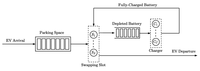
Figure 1: The mixed queuing network for a battery swapping station.

Consider the battery swapping station with $S$ automated swapping slots, $C$ chargers to recharge depleted batteries, $B$ batteries in circulation, and the queue capacity is $W$. Thus there are $W-S$ parking spots for awaiting EVs. Each battery swapping session lasts a constant service time $\tau_{s}$. The average arrival rate at each battery swapping station is $\bar{k}_{i,t}^{s}=(1-r_{i,t})k_{i,t}/\tilde{x}_{i,t}^{s}$. Assume that the EV arrival process is Poisson with rate $\bar{k}_{i,t}^{s}$. Let $g(u)$ denote the probability of having $u$ new-coming EVs during any time interval $(t,t+\tau_{s}]$. Based on the probability mass function of Poisson distribution, we derive $g(u)$ as

$$g(u)=\dfrac{(\bar{k}_{i,t}^{s}\tau_{s})^{u}\exp(-\bar{k}_{i,t}^{s}\tau_{s})}{u!},\,u\geq 0.$$ (13)

Further let $f(u,v)$ denote the probability of having $v$ batteries completing charging during $(t,t+\tau_{s}]$ provided that there are $u$ batteries being charged in the station at time $t$. Clearly, $f(u,v)$ is supported on $u\in[0,C]$ and $v\in[0,u]$. As aforementioned in the charging queue, suppose the battery charging time follows an independent and identical exponential distribution with parameter $1/\tau_{c}$. Then $f(u,v)$ is equivalent to having $v$ “success” in $u$ Bernoulli trials, each of which has a success probability $1-\exp(-\tau_{s}/\tau_{c})$:

$$f(u,v)=\begin{pmatrix}u\\ v\end{pmatrix}\left(1-\exp(-\tau_{s}/\tau_{c})\right)^{v}\exp(-(u-v)\tau_{s}/\tau_{c}).$$ (14)

With (13) and (14) respectively capturing the dynamics of EV arrival and battery circulation, we can proceed to establish the queuing equilibrium. The system can be characterized by a state tuple $(i,j)$ representing that there are $i$ EVs (including those waiting and being served) and $j$ fully-charged batteries in the station. Denote $G_{t}(i,j)$ as the probability of system state $(i,j)$ at time $t$ and denote $G_{t+\tau_{s}}(\hat{i},\hat{j})$ as the probability of system state $(\hat{i},\hat{j})$ at time $t+\tau_{s}$. We can then compute $G_{t+\tau_{s}}(\hat{i},\hat{j})$ given $G_{t}(i,j)$:

$$G_{t+\tau_{s}}(\hat{i},\hat{j})= \sum_{i=0}^{W}\sum_{j=0}^{B}G_{t}(i,j)g(\hat{i}-i+\Delta)f(B-j,\hat{j}-j+\Delta), \hat{i}<W$$ , (15a)

$$G_{t+\tau_{s}}(\hat{i},\hat{j})= \sum_{i=0}^{W}\sum_{j=0}^{B}G_{t}(i,j)\left(1-\sum_{d=1}^{W-1}g(d-i+\Delta)\right)f(B-j,\hat{j}-j+\Delta), \hat{i}=W$$ , (15b)

where $\Delta=\min\{i,j,S\}$ is the number of EVs leaving the station with fully-charged batteries during $(t,t+\tau_{s}]$. When the queue is not full at $t+\tau_{s}$, i.e., $\hat{i}<W$, the transition from $(i,j)$ to $(\hat{i},\hat{j})$ is equivalent to having $\hat{i}-i+\Delta$ EVs arriving and $\hat{j}-j+\Delta$ batteries finishing charging. However, if the queue capacity is reached, i.e., $\hat{i}=W$, there are at least $W-i-\Delta$ new arrivals during $(t,t+\tau_{s}]$, which happens with a probability of $1-\sum_{d=1}^{W-1}g(d-i+\Delta)$. The equilibrium state distribution, denoted as $G(i,j)=\lim_{t\rightarrow\infty}G_{t}(i,j)$, is given by solving (15b) together with the normalization equation $\sum_{i=0}^{W}\sum_{j=0}^{B}G(i,j)=1$. Note that the equation system consists of $(W+1)\times(B+1)+1$ linear equations but only $(W+1)\times(B+1)$ variables, which may not necessarily have a unique solution. Whereas it is proven in [63, Theorem 1] that the corresponding embedded Markov chain is ergodic. Thereby we can always find a unique equilibrium state distribution $G(i,j)$, based on which we can derive the average waiting time $w^{s}_{i,t}$. The expected queue length is $L=\sum_{i=0}^{W}\sum_{j=0}^{B}i\cdot G(i,j)$. Applying the Little’s law yields

$$L=\bar{k}_{s}(w^{s}_{i,t}+\tau_{s})\left(1-\sum_{j=0}^{B}G(W,j)\right),$$ (16)

where $1-\sum_{j=0}^{B}G(W,j)$ represents the probability that the queue is not full. Hence, the average waiting time at battery swapping stations is given by

$$w^{s}_{i,t}=\dfrac{\sum_{i=0}^{W}\sum_{j=0}^{B}i\cdot G(i,j)}{\bar{k}_{i,t}^{s}\left(1-\sum_{j=0}^{B}G(W,j)\right)}-\tau_{s}.$$ (17)

Due to the limited queue capacity, new-coming EVs at battery swapping stations could be blocked with a chance of $\sum_{j=0}^{B}G(W,j)$ and thus need to be dispatched to charging stations. However, this is not the primary focus of this work. To prevent the case of a full queue, we can choose a sufficiently large queue capacity $W$ such that the blocking rate is negligible for any EV arrival rate in a practical range. As shown in Figure 8, the blocking rate becomes nonnegligible only when swapping demand at each battery swapping station is very high. In this case, the waiting time is prohibitively long, which deters the platform from sending so many EVs for battery swapping. At equilibrium, swapping demand will be regulated in a reasonable regime so that facilities are not congested and the blocking rate is insignificant.

Remark 2.

In the proposed model, EVs are assumed to arrive at charging and battery swapping stations following a Poisson process, with an average arrival rate given by the stationary charging demand. This demand is derived using a random walk model in Section 3.3, which informs the average number of EVs that will need to recharge at equilibrium. We emphasize that the random walk model only provides inputs for the charging and battery swapping queues. The stochasticity of charging demand and capacity of charging facilities are encoded in the queuing models and reflected by the average waiting times, based on which the platform allocates limited resources over the infrastructure network for profit maximization.

3.5 Conservation of Time and Energy

The time of EVs or gasoline vehicles can be divided into several segments, including the time spent waiting for passengers, the time taken to pick up passengers, the time spent with a passenger on board, and the time spent in repositioning. For EVs, there is additional downtime associated with top-up events, including the time taken to charging infrastructure, the time spent waiting for an available facility, and the time spent in charging/battery swapping. Let $N^{e}_{t}$ and $N^{g}_{t}$ denote the total number of EVs and gasoline vehicles, respectively, then we can establish the time conservation for the entire fleet:

$$N^{g}_{t}=\sum_{i=1}^{M}N^{vg}_{i,t}+\sum_{i=1}^{M}\sum_{j=1}^{M}(1-R_{i,t})\left(\lambda_{ij,t}w^{p}_{i,t}+\lambda_{ij,t}\tau_{ij}+f_{ij,t}\tau_{ij}\right),$$ (18a)

$$N^{e}_{t}=\sum_{i=1}^{M}N^{ve}_{i,t}+\sum_{i=1}^{M}\sum_{j=1}^{M}R_{i,t}\left(\lambda_{ij,t}w^{p}_{i,t}+\lambda_{ij,t}\tau_{ij}+f_{ij,t}\tau_{ij}\right)$$

$$\quad\quad\quad+\sum_{i=1}^{M}r_{i,t}k_{i,t}(l^{c}_{i,t}+w^{c}_{i,t}+\tau_{c})+\sum_{i=1}^{M}(1-r_{i,t})k_{i,t}(l^{s}_{i,t}+w^{s}_{i,t}+\tau_{s}).$$ (18b)

The last two terms in (18b) account for the total number of EVs that are heading to, waiting at, and being served in charging and battery swapping stations.

In addition to time, the energy consumption of the entire EV fleet should also be balanced with the energy supply. Let $\omega$ denote the average electricity consumption rate and $\Omega$ denote the average battery capacity. In the long run, the electricity consumed by the entire EV fleet should match the total energy replenished through plug-in charging and battery swapping. This leads to the following energy balance condition:

$$\omega\left[\sum_{i=1}^{M}N^{ve}_{i,t}+\sum_{i=1}^{M}\sum_{j=1}^{M}R_{i,t}\big{(}\lambda_{ij,t}w^{p}_{i,t}+\lambda_{ij,t}\tau_{ij}+f_{ij,t}\tau_{ij}\big{)}+\sum_{i=1}^{M}r_{i,t}k_{i,t}l^{c}_{i}+\sum_{i=1}^{M}(1-r_{i,t})k_{i,t}l^{s}_{i,t}\right]=(1-\epsilon)\Omega\sum_{i=1}^{M}k_{i,t}$$ (19)

where $\epsilon$ is the average energy threshold below which an EV will top up the battery. In (19), the left-hand side of represents the total energy consumption, while the right-hand side represents the power input to the entire fleet. The first four terms on the left-hand side account for energy consumed by EVs in operations, while the last two terms correspond to energy consumed by EVs on their way to charging and battery swapping stations.

3.6 Profit Maximization

In the planning aspect, the platform decides when, where, and how many charging and battery swapping stations to build, while in the operation aspect, its decisions include ride fare, fleet composition, deployment and rebalancing policies, and charging mode choices. Note that planning decisions have long-term impacts, whereas operational decisions only depend on the availability of infrastructure in the current stage. Consider an infinite operation horizon and a $T$-stage planning horizon. The platforms makes these decisions in the planning horizon aimed at maximizing the total profit within the entire operation horizon. For notation brevity, we denote $x=[x_{1},\ldots,x_{T}]$ and $y=[y_{1},\ldots,y_{T}]$ as the planning and operational decisions of the platform, respectively. Recall that we have $x_{t}=[x_{t}^{c},x_{t}^{s}]$, where $x_{t}^{c}$ and $x_{t}^{s}$ are vectors that represent the number of charging stations and battery swapping stations to be built, respectively. We further have $y_{t}=[p_{t},N_{t},f_{t},r_{t}]$, where $p_{t}=[p_{1,t},\ldots,p_{M,t}]$ is the ride fare in each zone at stage $t$; $N_{t}=[N_{t}^{ve},N_{t}^{vg}]$, where $N_{t}^{ve}$ and $N_{t}^{vg}$ are the spatial distribution of idle EVs and gasoline vehicles, respectively; $f_{t}=[f_{ij,t}]_{\forall i,j=\{1,\ldots,M\}}$ is the matrix for rebalancing flow; and $r_{t}=[r_{1,t},\ldots,r_{M,t}]$ is the percentage of EVs assigned to charging stations in each zone. When decisions $x$ and $y$ are given, constraints (2)-(19) determines a set of endogenous variables. Under certain conditions, we can show that these endogenous variables are unique:

Proposition 2.

Given $x$ and $y$ satisfying (2) and (5)-(6), the stationary charging demand $k_{t}>0$ exists and is uniquely given by (3)-(4),(7b)-(9),(11) and (19) if

$$\dfrac{(1-\epsilon)\Omega}{\omega}-\sum_{i=1}^{M}r_{i,t}n_{i,t}l^{c}_{i,t}-\sum_{i=1}^{M}(1-r_{i,t})n_{i,t}l^{s}_{i,t}>0.$$ (20)

Proof.

For any $x$ and $y$, $0<n_{t}<1$ is uniquely determined by (9) based on Proposition 1. According to (10), $k_{t}>0$ exists as long as $\sum_{i=1}^{M}k_{i,t}>0$. Fix $x$ and $y$ and consider $K_{t}=\sum_{i=1}^{M}k_{i,t}>0$ as a variable. This reduces (19) to a linear equation with respect to $K_{t}$:

$$\left[\dfrac{(1-\epsilon)\Omega}{\omega}-\sum_{i=1}^{M}r_{i,t}n_{i,t}l^{c}_{i,t}-\sum_{i=1}^{M}(1-r_{i,t})n_{i,t}l^{s}_{i,t}\right]K_{t}=\sum_{i=1}^{M}N^{ve}_{i,t}+\sum_{i=1}^{M}\sum_{j=1}^{M}R_{i,t}\left(\lambda_{ij,t}w^{p}_{i,t}+\lambda_{ij,t}\tau_{ij}+f_{ij,t}\tau_{ij}\right).$$

Since right-hand side is positive, the above equation has a strictly positive solution only when (20) holds. ∎

This condition implies that the charging mode choice $r$ should be properly made in accordance with other operational decisions so that the energy balance condition can be satisfied. So far, we have characterized how the platform’s decisions affect the endogenous charging demand. Specifically, (9) reveals the charging demand distribution at equilibrium, and (19) provides a scaling factor for (9) to ensure that the energy input and output are balanced. Given any feasible planning decisions $x$ and operational decisions $y$, we can always uniquely compute the charging demand $k_{t}$, which further determines the queuing times at charging and battery swapping stations through (12)-(17) and consequently decides the fleet size through (18b).

To characterize the profit-maximization problem of the ride-hailing platform, we denote $\gamma_{g}$ and $\gamma_{e}$ as the per-unit-time operational cost of gasoline vehicles and EVs, and further denote $\gamma_{c}$ and $\gamma_{s}$ as the operational cost of each charging and battery swapping stations. At each stage, the platform’s revenue is

$$\Pi^{r}_{t}=\sum_{i=1}^{M}\sum_{j=1}^{M}p_{i,t}\lambda_{ij,t}\tau_{ij}.$$ (21)

While the platform’s expenditures consist of the deployment cost of charging facilities and the operational costs for both the ride-hailing fleet and the infrastructure network:

$$\Pi^{dc}_{t} =a_{c}\sum_{i=1}^{M}x_{i,t}^{c}+a_{s}\sum_{i=1}^{M}x_{i,t}^{s},$$ (22a)

$$\Pi^{oc}_{t} =\gamma_{g}N^{g}_{t}+\gamma_{e}N^{e}_{t}+\gamma_{c}\sum_{i=1}^{M}\tilde{x}_{i,t}^{c}+\gamma_{s}\sum_{i=1}^{M}\tilde{x}_{i,t}^{s},$$ (22b)

where $\Pi^{dc}_{t}$ is the deployment cost and $\Pi^{oc}_{t}$ is the operational cost. Note that we do not explicitly factor in the different purchase costs of EVs and gasoline cars for two main reasons. Firstly, given the steadily falling prices of EVs and the increasing government incentives, it is expected that the prices of EVs will be comparable to those of their gasoline-powered counterparts. Secondly, the price difference can be indirectly accounted for by amortizing the purchase costs on an hourly basis and incorporating them into the operational costs.

Since the platform stops building charging infrastructure after stage $T$, the deployment cost is removed thereafter, and the platform’s revenue and operational costs remain unchanged from stage $T+1$ onward. To trade off the short-term and long-term performance of different deployment strategies, we introduce a discount factor $\sigma\in(0,1)$. The total profit is then defined as

$$\begin{split}\Pi&=\sum_{t=1}^{T}\sigma^{t-1}(\Pi^{r}_{t}-\Pi^{dc}_{t}-\Pi^{oc}_{t})+\sum_{t=T+1}^{\infty}\sigma^{t-1}(\Pi^{r}_{T}-\Pi^{oc}_{T})\\ &=\sum_{t=1}^{T}\sigma^{t-1}(\Pi^{r}_{t}-\Pi^{dc}_{t}-\Pi^{oc}_{t})+\dfrac{\sigma^{T}}{1-\sigma}(\Pi^{r}_{T}-\Pi^{oc}_{T}).\end{split}$$ (23)

Let $\hat{x}=[\hat{x}^{c}_{i},\ldots,\hat{x}^{c}_{M},\hat{x}^{s}_{i},\ldots,\hat{x}^{s}_{M}]$ be the maximum number of facilities allowed to deploy in each zone because of practical restrictions, e.g., limited land supply. Let $\hat{N}^{v}>0$ be the lower bound for the total number of idle vehicles in each zone, which accounts for the practice that the platform will maintain the vehicle supply above a certain threshold to ensure service quality. The platform’s profit maximization problem is formulated as follows:

$$\underset{x_{1},y_{1},\cdots,x_{T},y_{T}}{\text{maximize}}\quad \sum_{t=1}^{T}\sigma^{t-1}(\Pi^{r}_{t}-\Pi^{dc}_{t}-\Pi^{oc}_{t})+\dfrac{\sigma^{T}}{1-\sigma}(\Pi^{r}_{T}-\Pi^{oc}_{T})$$ (24a)

subject to $$\eqref{eqn:expansion}-\eqref{eqn:energy balance},$$

$$0\leq\sum_{\tau=1}^{t}x_{\tau}\leq\hat{x},\ \forall t\in\{1,\cdots,T\},$$ (24b)

$$N^{ve}_{i,t}+N^{vg}_{i,t}\geq\hat{N}^{v},\ \forall t\in\{1,\cdots,T\},i\in\{1,\cdots,M\},$$ (24c)

$$\dfrac{(1-\epsilon)\Omega}{\omega}-\sum_{i=1}^{M}r_{i,t}n_{i,t}l^{c}_{i,t}-\sum_{i=1}^{M}(1-r_{i,t})n_{i,t}l^{s}_{i,t}>0,\ \forall t\in\{1,\cdots,T\},$$ (24d)

which is a multi-stage optimization over a transportation network. It is worth noting that the deployment of charging infrastructure will introduce a cost term in the objective function (24a), while also being subject to the budgetary constraint (2). In this formulation, travel time $l^{c}_{i,t}$ and $l^{s}_{i,t}$, pickup time $w^{p}_{i,t}$, passenger demand $\lambda_{ij,t}$, charging demand $k_{i,t}$, charging waiting time $w^{c}_{i,t}$, and swapping waiting time $w^{s}_{i,t}$ are endogenous variables that are given by (1b)-(19).

Remark 3.

Typically ride-hailing EV drivers choose their charging modes to minimize their own downtime. Nonetheless, since the time required for battery swapping is significantly shorter than plug-in charging, drivers tend to overuse battery swapping, leading to congested swapping stations but under-utilized charging stations. This would undermine the benefits of introducing battery swapping stations in the first place. As a result, the platform must motivate drivers to use battery swapping facilities appropriately to ensure that the charging mode choice is close to the system-level optimal, as in the proposed model. Even without direct control over the fleet, the platform can still achieve this through indirect measures such as limiting the queuing capacity of battery swapping stations, providing incentives for using recommended charging modes, introducing reservation-based battery swapping services, etc. However, a detailed study of these indirect measures is beyond the scope of this paper and thus we leave it for future research.

4 Solution Method

Due to the nonconvexity of (24), it is inherently challenging to pinpoint its globally optimal solution. Standard nonlinear programming algorithms (such as interior-point methods) can produce a feasible solution but without offering any verifiable performance guarantee. In this light, we relax and reformulate the original problem into a decomposable one, based on which an upper bound can be established to evaluate the solution optimality.

4.1 Relaxation and Reformulation

Temporal Dimension: Any planning decision at stage $t$ will directly affect the infrastructure network at all subsequent stages, resulting in interdependence among different stages. To decouple the temporal correlation, we directly use $\tilde{x}_{t}=\sum_{\tau=1}^{t}x_{\tau}$ to replace $x_{t}$ as a decision variable. The change of variables does not affect the budgetary constraint (2). While extra inequality constraints should be introduced to guarantee the deployment decision at each stage is nonnegative:

$$\tilde{x}_{t}-\tilde{x}_{t-1}\geq 0,\ \forall t\in\{1,\cdots,T\},$$ (25)

which is equivalent to enforcing a lower bound on $\tilde{x}_{t}$ based on the existing infrastructure network $\tilde{x}_{t-1}$. As such, the correlation over stages is embedded in a set of inequality constraints (25), which significantly simplifies the formulation in the temporal dimension.

Spatial Dimension: The original formulation (24) involves a complex decision making process over the network. To enhance the tractability, we further simplify the problem in the spatial dimension. We first note that the flow balance constraint (5) couples the decisions of distinct zones. In ride-hailing markets, however, popular pickup locations are typically popular trip destinations, thus the passenger inflow is naturally close to the outflow even without rebalancing. Following this intuition, we relax the original formulation (24) by removing the flow balance constraint (5). Note that we do not eliminate the rebalancing flow $f_{t}$ in other formulas, e.g., (7b), (19) and (18b). The platform can still adjust $f_{t}$ to steer charging demand but with more freedom, since the decision is no longer subject to the flow balance condition. Therefore, the relaxed problem offers an upper bound for the original problem.

Another complexity arises from the charging demand model. Charging demand in each zone not only depends on local operational decisions but also relies on decisions for all other zones. To see this, we combine (9) and (10) to derive the following equations:

$$\begin{split}&k_{1,t}P_{11,t}+k_{2,t}P_{21,t}+\cdots+k_{M,t}P_{M1,t}=\sum_{i=1}^{M}k_{i,t}P_{i1,t}=k_{1,t},\\ &\quad\quad\quad\quad\quad\quad\vdots\\ &k_{1,t}P_{1M,t}+k_{2,t}P_{2M,t}+\cdots+k_{M,t}P_{MM,t}=\sum_{i=1}^{M}k_{i,t}P_{iM,t}=k_{M,t},\end{split}$$ (26)

where $P_{ij,t}$ corresponds to the $(i,j)$-entry in the transition matrix established in (8). Recall that $k_{t}$ is endogenous and $P_{ij,t}$ is a function of $y_{t}$. It is clear that these equations relate operational decisions for different zones to each other. To disentangle the spatial interdependence, we include charging demand $k_{t}>0$ as decision variables and define the augmented operational decision as $\tilde{y}=[\tilde{y}_{1}\ldots,\tilde{y}_{T}]$, where $\tilde{y}_{t}=[p_{t},N_{t},f_{t},r_{t},k_{t}]$. As such, the modified optimization is subject to extra equality constraints (26), energy balance condition (19), and an additional positivity constraint (27d) that replaces the feasibility condition (20). We emphasize that this modification does not reflect the real-world practice as charging demand is endogenously and uniquely determined by the platform’s operation strategy. The augmentation of decisions is to decouple the spatial correlation, transform the optimization to a decomposable one, and thus facilitate further analysis. After the aforementioned modifications, the original problem (24) is reformulated as follows:

$$\underset{\tilde{x}_{1},\tilde{y}_{1},\cdots,\tilde{x}_{T},\tilde{y}_{T}}{\text{maximize}}\quad \sum_{t=1}^{T}\sigma^{t-1}(\Pi^{r}_{t}-\Pi^{dc}_{t}-\Pi^{oc}_{t})+\dfrac{\sigma^{T}}{1-\sigma}(\Pi^{r}_{T}-\Pi^{oc}_{T})$$ (27a)

subject to $$\eqref{eqn:budget}-\eqref{eqn:pickup time},\eqref{eqn:EV deployment}-\eqref{eqn:energy balance},$$

$$0\leq\tilde{x}_{t}\leq\hat{x},\ \forall t\in\{1,\cdots,T\},$$ (27b)

$$\tilde{x}_{t}-\tilde{x}_{t-1}\geq 0,\ \forall t\in\{1,\cdots,T\},$$ (27c)

$$k_{i,t}>0,\ \forall t\in\{1,\cdots,T\},i\in\{1,\cdots,M\},$$ (27d)

$$N^{ve}_{i,t}+N^{vg}_{i,t}\geq\hat{N}^{v},\ \forall t\in\{1,\cdots,T\},i\in\{1,\cdots,M\},$$ (27e)

$$\sum_{j=1}^{M}k_{j,t}P_{ji,t}-k_{i,t}=0,\ \forall t\in\{1,\cdots,T\},i\in\{1,\cdots,M-1\}$$ (27f)

Note that constraint (27f) is for zone $1$ to $M-1$. This is because the charging demand model (26) involves a total of $M$ interdependent equations. Without loss of generality, we exclude the equation for zone $M$ to guarantee the gradients of these equality constraints are linearly independent such that the Lagrange multiplier associated with (27f) exists [64]. Overall, the reformulated problem (27) is equivalent to the original problem (24) except that the flow balance condition is dropped. The change of variables does not affect other constraints in (24). To see this, we sum up the $M-1$ equations in (27f) over $i$ for some stage $t$ and obtain

$$\begin{split}&k_{1,t}\sum_{i=1}^{M-1}P_{1i,t}+k_{2,t}\sum_{i=1}^{M-1}P_{2i,t}+\cdots+k_{M,t}\sum_{i=1}^{M-1}P_{Mi,t}-\sum_{i=1}^{M-1}k_{i,t}\\ =\ &k_{1,t}(1-P_{1M,t})+k_{2,t}(1-P_{2M,t})+\cdots+k_{M,t}(1-P_{MM,t})-\sum_{i=1}^{M}k_{i,t}+k_{M,t}\\ =\ &k_{M,t}-(k_{1,t}P_{1M,t}+k_{2,t}P_{2M,t}+\cdots+k_{M,t}P_{MM,t})=0.\end{split}$$ (28)

This is the same as the last equation in (26), showing that constraints (27f) are equivalent to the charging demand model. Hence, (27) is a relaxed reformulation of the original problem (24) and the optimal solution to (27) provides an upper bound for (24).

4.2 Decomposition and Upper Bound

Compared to the original problem, the reformulation remains nonconvex but presents a decomposable structure, which can be used to examine the solution optimality. For ease of notation, we denote the combination of (27f) and (19) as $h_{t}(\tilde{x}_{t},\tilde{y}_{t})=0$, where $h_{t}(\tilde{x}_{t},\tilde{y}_{t})=[h_{1,t}(\tilde{x}_{t},\tilde{y}_{t}),\ldots,h_{M,t}(\tilde{x}_{t},\tilde{y}_{t})]$ is an $M$-dimensional vector-valued function. Particularly, $h_{m,t}(\tilde{x}_{t},\tilde{y}_{t})=\sum_{i=1}^{M}h_{mi,t}(\tilde{x}_{i,t},\tilde{y}_{i,t})$, where

$$h_{mi,t}(\tilde{x}_{i,t},\tilde{y}_{i,t})= k_{i,t}\left[(1-\epsilon)\Omega/\omega-r_{i,t}l^{c}_{i,t}-(1-r_{i,t})l^{s}_{i,t}\right]-N^{ve}_{i,t}$$

$$h_{mi,t}(\tilde{x}_{i,t},\tilde{y}_{i,t})= \quad\quad-\sum_{j=1}^{M}R_{i,t}(\lambda_{ij,t}w^{p}_{i,t}+\lambda_{ij,t}\tau_{ij}+f_{ij,t}\tau_{ij}), m=M$$ , (29a)

$$h_{mi,t}(\tilde{x}_{i,t},\tilde{y}_{i,t})= k_{i,t}\tilde{P}_{im,t}, m<M$$ , (29b)

and $\tilde{P}_{t}=P_{t}-I$, with $I$ denoting an identity matrix. We emphasize that based on (7b) and (8), $\tilde{P}_{im,t}$ only depends on the decision variables for zone $i$. Therefore, the right-hand side of (29b) can be expressed solely as a function of $\tilde{x}_{i,t}$ and $\tilde{y}_{i,t}$, which does not depend on the decision variables for other zones. In addition, we observe that $\Pi^{r}_{t}$, $\Pi^{dc}_{t}$, and $\Pi^{oc}_{t}$ in the objective function (27a) can be expressed as a summation over zones (see (18b)(21)(22)). Hence, (27a) can be rewritten as

$$\Pi=\sum_{t=1}^{T}\sigma^{t-1}(\Pi^{r}_{t}-\Pi^{dc}_{t}-\Pi^{oc}_{t})+\dfrac{\sigma^{T}}{1-\sigma}(\Pi^{r}_{T}-\Pi^{oc}_{T})=\sum_{t=1}^{T}\sum_{i=1}^{M}\Pi_{i,t}.$$

The reformulated problem then becomes

$$\underset{\tilde{x}_{1},\tilde{y}_{1},\cdots,\tilde{x}_{T},\tilde{y}_{T}}{\text{maximize}}\quad \sum_{t=1}^{T}\sum_{i=1}^{M}\Pi_{i,t}$$ (30a)

subject to $$\eqref{eqn:budget}-\eqref{eqn:pickup time},\eqref{eqn:EV deployment}-\eqref{eqn:fleet size},$$

$$0\leq\tilde{x}_{t}\leq\hat{x},\ \forall t\in\{1,\cdots,T\},$$ (30b)

$$\tilde{x}_{t}-\tilde{x}_{t-1}\geq 0,\ \forall t\in\{1,\cdots,T\},$$ (30c)

$$k_{i,t}>0,\ \forall t\in\{1,\cdots,T\},i\in\{1,\cdots,M\},$$ (30d)

$$N^{ve}_{i,t}+N^{vg}_{i,t}\geq\hat{N}^{v},\ \forall t\in\{1,\cdots,T\},i\in\{1,\cdots,M\},$$ (30e)

$$\sum_{i=1}^{M}h_{mi,t}(\tilde{x}_{i,t},\tilde{y}_{i,t})=0,\ \forall m\in\{1,\cdots,M\},t\in\{1,\cdots,T\}.$$ (30f)

As such, only the budgetary constraint (2), nonnegativity constraints (30c), and charging demand constraints (30f) are coupled. We can thus decompose (30) into multiple small-scale subproblems, each of which corresponds to the decision for a zone at a stage. Let $(\mu,\eta,\theta)$ be the Lagrange multipliers associated with constraints (2), (30c), and (30f). The partial Lagrangian reads as follows:

$$\mathcal{L}(\tilde{x},\tilde{y})\Big{|}_{\mu,\eta,\theta}=\sum_{t=1}^{T}\left[\sum_{i=1}^{M}\Pi_{i,t}+\mu_{t}\left(\tilde{b}_{t}-\sum_{i=1}^{M}A_{i}^{\top}\tilde{x}_{i,t}\right)+\sum_{i=1}^{M}\eta_{i,t}^{\top}\left(\tilde{x}_{i,t}-\tilde{x}_{i,t-1}\right)+\sum_{m=1}^{M}\sum_{i=1}^{M}\theta_{m,t}h_{mi,t}(\tilde{x}_{i,t},\tilde{y}_{i,t})\right],$$ (31)

where $A_{i}=[a_{c},a_{s}]$ and $\tilde{x}_{i,t}=[\tilde{x}^{c}_{i,t},\tilde{x}^{s}_{i,t}]$. Clearly, given the Lagrange multipliers, the Lagrangian is separable in both spatial and temporal dimensions after ignoring the constant term, i.e.,

$$\mathcal{L}(\tilde{x},\tilde{y})\Big{|}_{\mu,\eta,\theta}=\sum_{t=1}^{T}\sum_{i=1}^{M}\mathcal{L}_{i,t}(\tilde{x}_{i,t},\tilde{y}_{i,t})\Big{|}_{\mu_{t},\eta_{i,t},\theta_{t}},$$

where $\mathcal{L}_{i,t}$ is obtained by plugging (18b),(21),(22), and (29b) into (31). Thus we can separately optimize the following subproblem for stage $t$ and zone $i$:

$$\underset{\tilde{x}_{i,t},\tilde{y}_{i,t}}{\text{maximize}}\quad \mathcal{L}_{i,t}(\tilde{x}_{i,t},\tilde{y}_{i,t})\Big{|}_{\mu_{t},\eta_{i,t},\theta_{t}}$$ (32a)

subject to $$\eqref{eqn:demand model}-\eqref{eqn:pickup time},\eqref{eqn:EV deployment}-\eqref{eqn:swapping queue},$$

$$0\leq\tilde{x}_{i,t}\leq\hat{x}_{i},$$ (32b)

$$k_{i,t}>0,$$ (32c)

$$N^{ve}_{i,t}+N^{vg}_{i,t}\geq\hat{N}^{v},$$ (32d)

which includes $\tilde{x}_{i,t}=[\tilde{x}^{c}_{i,t},\tilde{x}^{s}_{i,t}]$ and $\tilde{y}_{i,t}=[p_{i,t},N^{ve}_{i,t},N^{vg}_{i,t},r_{i,t},k_{i,t},f_{i1,t},\ldots,f_{iM,t}]$ as decision variables.

Note that (32) still remains nonconvex. To find its globally optimal solution, we introduce a new decision $\tilde{f}_{i,t}\geq 0$ and equivalently rewrite (32) as

$$\underset{\tilde{x}_{i,t},\tilde{y}_{i,t},\tilde{f}_{i,t}}{\text{maximize}}\quad \mathcal{L}_{i,t}(\tilde{x}_{i,t},\tilde{y}_{i,t})\Big{|}_{\mu_{t},\eta_{i,t},\theta_{t}}$$ (33a)

subject to $$\eqref{eqn:demand model}-\eqref{eqn:pickup time},\eqref{eqn:EV deployment}-\eqref{eqn:swapping queue},$$

$$0\leq\tilde{x}_{i,t}\leq\hat{x}_{i},$$ (33b)

$$k_{i,t}>0,$$ (33c)

$$N^{ve}_{i,t}+N^{vg}_{i,t}\geq\hat{N}^{v},$$ (33d)

$$\sum_{j=1}^{M}f_{ij,t}\tau_{ij}=\tilde{f}_{i,t},$$ (33e)

where constraint (33e) is introduced to account for the definition of $\tilde{f}_{i,t}$. To facilitate the discussion, we re-group the decision variables as $\bar{x}_{i,t}=[\tilde{x}^{c}_{i,t},\tilde{x}^{s}_{i,t},f_{i1,t},\ldots,f_{iM,t}]$ and $\bar{y}_{i,t}=[p_{i,t},N^{ve}_{i,t},N^{vg}_{i,t},r_{i,t},k_{i,t},\tilde{f}_{i,t}]$.

In order to establish an upper bound for the original problem, we must obtain the globally optimal solution to (33). However, the subproblem (33) is nonconvex and involves a high-dimensional decision space, including $(M+2)$-dimensional $\bar{x}_{i,t}$ and six-dimensional $\bar{y}_{i,t}$. Fortunately, we observe that given $\bar{y}_{i,t}$, the problem is concave with respect to $\bar{x}_{i,t}$. To show this, we hold $\bar{y}_{i,t}$ as constant, ignore all the constant terms in $\mathcal{L}_{i,t}(\tilde{x}_{i,t},\tilde{y}_{i,t})$, and write down $\mathcal{L}_{i,t}$ as a function of $\bar{x}_{i,t}$:

$$\mathcal{L}_{i,t}(\bar{x}_{i,t})= -\sigma^{t-1}\left[\gamma_{e}r_{i,t}k_{i,t}(l^{c}_{i,t}+w^{c}_{i,t})+\gamma_{e}(1-r_{i,t})k_{i,t}(l^{s}_{i,t}+w^{s}_{i,t})+\Gamma^{\top}\tilde{x}_{i,t}\right]$$

$$\mathcal{L}_{i,t}(\bar{x}_{i,t})= \quad\quad-(\sigma^{t-1}-\sigma^{t})A_{i}^{\top}\tilde{x}_{i,t}-\mu_{t}A_{i}^{\top}\tilde{x}_{i,t}+(\eta_{i,t}-\eta_{i,t+1})^{\top}\tilde{x}_{i,t} t<T$$ (34a)

$$\mathcal{L}_{i,t}(\bar{x}_{i,t})= \quad\quad+\sum_{m=1}^{M-1}\theta_{m,t}k_{i,t}\tilde{P}_{im,t}-\theta_{M,t}\left[r_{i,t}k_{i,t}l^{c}_{i,t}+(1-r_{i,t})k_{i,t}l^{s}_{i,t}\right],$$

$$\mathcal{L}_{i,t}(\bar{x}_{i,t})= \frac{-\sigma^{t-1}}{1-\sigma}\left[\gamma_{e}r_{i,t}k_{i,t}(l^{c}_{i,t}+w^{c}_{i,t})+\gamma_{e}(1-r_{i,t})k_{i,t}(l^{s}_{i,t}+w^{s}_{i,t})+\Gamma^{\top}\tilde{x}_{i,t}\right]$$

$$\mathcal{L}_{i,t}(\bar{x}_{i,t})= \quad\quad-\sigma^{t-1}A_{i}^{\top}\tilde{x}_{i,t}-\mu_{t}A_{i}^{\top}\tilde{x}_{i,t}+\eta_{i,t}^{\top}\tilde{x}_{i,t} t=T$$ (34b)

$$\mathcal{L}_{i,t}(\bar{x}_{i,t})= \quad\quad+\sum_{m=1}^{M-1}\theta_{m,t}k_{i,t}\tilde{P}_{im,t}-\theta_{M,t}\left[r_{i,t}k_{i,t}l^{c}_{i,t}+(1-r_{i,t})k_{i,t}l^{s}_{i,t}\right],$$

where $\Gamma=[\gamma_{c},\gamma_{s}]$. Note that in (4.2), $r_{i,t}$ and $k_{i,t}$ are fixed. As a result, $l^{c}_{i,t}$ and $w^{c}_{i,t}$ depend on $\tilde{x}^{c}_{i,t}$, $l^{s}_{i,t}$ and $w^{s}_{i,t}$ depend on $\tilde{x}^{s}_{i,t}$, and $\tilde{P}_{im,t}$ depends on $[f_{i1,t},\ldots,f_{iM,t}]$. In order for (4.2) to be a concave function with respect to $\bar{x}_{i,t}$, we need all the aforementioned dependencies to be convex (note the negative coefficient $-\gamma_{e}$, and that $\theta_{M,t}\geq 0$.). According to (11), $l^{c}_{i,t}$ and $l^{s}_{i,t}$ are respectively convex in $\tilde{x}^{c}_{i,t}$ and $\tilde{x}^{s}_{i,t}$. Additionally, based on (7b) and (8), when $p_{i,t}$, $N^{ve}_{i,t}$, $N^{vg}_{i,t}$, $r_{i,t}$, and $\tilde{f}_{i,t}=\sum_{j=1}^{M}f_{ij,t}\tau_{ij}$ are held fixed, the denominator of $\tilde{P}_{im,t}$ is also fixed, while the enumerator is linear with respect to $f_{im,t}$. Consequently, $\tilde{P}_{im,t}$ is linear function of $f_{im,t}$. Furthermore, the waiting time in an M/M/N queue has been proved to be convex with respect to the number of servers in [65], which ensures the convexity of $w^{c}_{i,t}$. Lastly, we argue that $w^{s}_{i,t}$ is also convex with respect to $\tilde{x}^{s}_{i,t}$. The reasoning is straightforward: when $\bar{y}_{i,t}$ is fixed, the arrival rate at each battery swapping station is also determined. In this case, building more battery swapping stations will alleviate congestion and reduce the waiting time, i.e., $w^{s}_{i,t}$. However, the marginal benefit of building more infrastructure will diminish as the network further expands, implying that $w^{s}_{i,t}$ is decreasing and convex in $\tilde{x}^{s}_{i,t}$. Due to the intricate queuing model, it is difficult to analytically prove its convexity. Instead, the convexity is numerically validated in A through a comprehensive sensitivity analysis.

Overall, for any given $\bar{y}_{i,t}$, (4.2) is a concave function of $\bar{x}_{i,t}$ and therefore the subproblem (32) becomes a concave optimization that can be efficiently solved. Hence, we propose to obtain the globally optimal solution to (33) through a hierarchical approach, where we first apply grid search over $\bar{y}_{i,t}$ and then for each fixed $\bar{y}_{i,t}$ we find the corresponding optimal $\bar{x}_{i,t}$ by solving a convex program. At last, we will compare the obtain optimal value for distinct values of $\bar{y}_{i,t}$ and find the maximum. Note that the dimensionality of $\bar{y}_{i,t}$ is small and does not depend on the number of zones. Based on the weak duality theorem, for any Lagrange multipliers $(\mu,\eta,\theta)$, solutions to all subproblems collectively provide a valid upper bound for the reformulated problem (27). This upper bound can be further improved by iteratively updating the Lagrange multipliers in a dual decomposition framework with the following update rule:

$$\mu_{t}\leftarrow\max\{0,\mu_{t}-\zeta(\tilde{b}_{t}-A^{\top}\tilde{x}_{t})\},$$ (35a)

$$\eta_{i,t}\leftarrow\max\left\{0,\eta_{i,t}-\zeta\left(\tilde{x}_{i,t}-\tilde{x}_{i,t-1}\right)\right\},$$ (35b)

$$\theta_{m,t}\leftarrow\theta_{m,t}-\zeta h_{mi,t}(\tilde{x}_{i,t},\tilde{y}_{i,t}),$$ (35c)

where $\zeta$ is the step size. Since the flow balance condition is dropped in (27), the established upper bound further overestimates the globally optimal solution to the original problem (24). This enables us to quantify the solution optimality for (24). We summarize the procedure as follows:

• Step 1: Solve the original problem (24) via nonlinear programming solvers and find a feasible solution. This solution provides a valid lower bound for (24).

• Step 2: Solve the relaxed and reformulated problem (27) via nonlinear programming solvers and obtain the corresponding Lagrange multipliers $(\mu,\eta,\theta)$.

• Step 3: Plug $(\mu,\eta,\theta)$ into (32). For each subproblem, enumerate $\bar{y}_{i,t}$ and solve the residual concave problem. Find the globally optimal solutions to all subproblems.

• Step 4: Combine subproblems’ solutions to establish a valid upper bound for (24). Evaluate the bound performance by measuring the gap between lower and upper bounds.

• Step 5: Terminate the procedure if the optimality gap is satisfactorily tight. Otherwise, update the multipliers according to (35c) and go to Step 3.

The aforementioned procedure can be terminated after any number of iterations, and no matter when it is terminated, the derived bound is always a valid upper bound for the original problem. The proposed algorithm is an example of how the special structure of the problem can be exploited to evaluate the solution optimality of a highly nonconvex optimization problem, given that a solution can be derived by some other gradient-based nonlinear programming solvers. We emphasize that the proposed method is nontrivial and rather useful. Because for most large-scale nonconvex problems, it is not difficult to use nonlinear programming solvers to find a local solution, but it is very difficult to examine how good the solution is compared to the unknown globally optimal one. In this work, we tackle this intrinsic challenge by leveraging the special problem structure and reformulating the joint deployment problem as a decomposable one. We show, through a series of manipulations, that each subproblem becomes concave when a part of decisions is temporarily held fixed. This enables us to efficiently solve all the subproblems and construct an upper bound for the original problem, thus making it possible to validate whether the obtained solution is close enough to the globally optimal one. Put simply, our method makes the solution optimality of (24) verifiable despite its nonconvexity.

5 Numerical Studies

Based on the proposed formulation and analytical analysis, this section presents several case studies to validate the solution optimality and discuss the effectiveness of the joint deployment scheme.

5.1 Simulation Settings

A series of case studies are conducted for Manhattan, New York City, where a platform jointly deploys charging infrastructure and operates a ride-hailing fleet. The island is divided into 20 zones. Real data from the New York City Taxi and Limousine Commission (NYCTLC) [66] was used to estimate travel demand, including pickup and dropoff locations as well as trip duration. The demand function in (3) is materialized as a binary logit model:

$$\lambda_{ij,t}=\bar{\lambda}_{ij}\dfrac{\exp(-\varepsilon c_{ij,t})}{\exp(-\varepsilon c_{ij,t})+\exp(-\varepsilon c^{0}_{ij})},$$ (36)

where $\varepsilon>0$ is a sensitivity parameter, $c_{ij,t}=p_{i,t}\tau_{ij}+\alpha w^{p}_{i,t}$ represents the generalized cost of a type-$(i,j)$ trip, and $c^{0}_{ij}$ represents the cost of outside options. Particularly, we assume $c^{0}_{ij}$ to be proportional to the trip duration, i.e., $c^{0}_{ij}=p_{0}\tau_{ij}$.

Consider a four-stage infrastructure investment plan, i.e., $T=4$. To capture the entire expansion process of an infrastructure network, we define $\tilde{x}_{0}^{c}=0$ and $\tilde{x}_{0}^{s}=0$, implying that there is no charging facility before the first planning stage. Given the practical observation that building and operating battery swapping stations is significantly more expensive than charging stations, we assume that the deployment and operational costs of each charging station are $a_{c}=\$20/\text{hr}$ and $\gamma_{c}=\$2/\text{hr}$, respectively, while both costs of each battery swapping station are ten times that of a charging station. The discount factor in (23) is set as 95%. Parameters related to ride-hailing operations, including $(\phi,\psi,\alpha,\epsilon,\varepsilon,p_{0},\gamma_{e},\gamma_{g})$, are calibrated via reverse engineering with partial reference to [56] such that the proposed model reproduces an equilibrium solution that is close to empirical data. Specifically, to reflect the economical efficiency of EVs, we set the operational costs of each EV and gasoline car as $\gamma_{e}=\$15/\text{hr}$ and $\gamma_{g}=\$20/\text{hr}$. On the other hand, parameters related to EVs and infrastructure are calibrated to match the industry practice. In (19), instead of tuning $(\epsilon,\omega,\Omega)$ separately, we fix $(1-\epsilon)\Omega/\omega=8$, meaning that EVs can sustain for eight hours between two top-ups. This follows from the charging pattern of a large-scale electric taxi fleet [67]. As for infrastructure, we assume all charging/battery swapping stations share the same specifications. Each charging station is equipped with $V=5$ chargers. Each battery swapping station has $S=1$ swapping machine, $C=5$ chargers, $B=5$ batteries, and has a queue capacity of $W=50$. The average charging time is $t_{c}=1$ hour, and each swapping session lasts $t_{s}=5$ minutes.

5.2 Performance of the Upper Bound

Table 1: Solution optimality under different simulation settings.

Totl. Budget	Demand Pattern	# of Zones	LB	UB	Gap	Totl. Comp. Time (min)	Avg. Subprob. Comp. Time (min)
40	24-Hr Avg.	20	44326.19	47300.04	6.29%	4095.00	51.19
60	24-Hr Avg.	20	44876.02	47666.38	5.85%	3985.41	49.82
40	Peak Hr.	20	62226.28	67893.83	8.35%	4132.82	51.66
60	Peak Hr.	20	63005.84	68103.66	7.49%	4239.27	52.99
40	24-Hr Avg.	6	41697.96	43830.61	4.87%	1595.48	66.48
60	24-Hr Avg.	6	42259.51	44574.48	5.19%	1608.83	67.03

The solution optimality is evaluated across various budget levels, demand patterns, and network sizes. The total budget is quantified in terms of the number of swapping stations, for ease of comprehension. The average demand in a 24-hour period is utilized as the benchmark for evaluation. To investigate the impact of relaxing the flow balance constraint, we test the performance during peak hours (e.g., 7 pm), when passenger inflow and outflow of each zone are more imbalanced. In addition, we include the solution optimality for a six-zone network, which will be used in the subsequent section to visualize the expansion process of infrastructure network.

Feasible solutions to (24) serve as lower bounds, while solutions to (32) provide upper bounds, as previously mentioned. We utilize interior-point methods in steps 1 and 2 of our proposed solution procedure. Simulations are conducted using MATLAB on a workstation equipped with a 64-core Intel Xeon Platinum CPU. Table 1 reports the optimality gap and the computation time of Step 3 after one iteration, which is the most time-consuming component in the proposed method. Our results indicate that the proposed method performs consistently well in different settings. Using the multipliers in step 2 without further updates can produce a tight upper bound with an optimality gap of approximately 6%, showing that a near-optimal solution to (24) is attained. As expected, the gap increases during peak hours due to the relaxation of the flow balance constraint, which enables the platform to fully utilize the fleet to provide services. Nevertheless, the gap remains within an acceptable range of around 8%, underscoring the effectiveness of our approach in the case of spatially asymmetric demand. Besides, compared to the 6-zone network, the 20-zone one produces a larger optimality gap, because it results in an optimization problem with much more decision variables and constraints. The problem scale affects the solution quality and Lagrange multipliers in step 2, consequently influencing the bound performance. However, the average computation time for each subproblem is shorter in the 20-zone case due to the narrower search range of decision variables, such as the number of idle vehicles in each zone ($N^{ve}_{i,t}$ and $N^{vg}_{i,t}$). Moreover, deriving an upper bound typically requires days of computation time, depending on the network scale. However, we emphasize that the infrastructure planning problem does not require real-time computation. The computation time is orders of magnitude shorter than the implementation time of a deployment plan (e.g., in the range of months or years), rendering it insignificant for the planning purpose.

5.3 Synergy between Charging and Battery Swapping

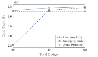
Figure 2: The platform’s total profit under varying budget levels.

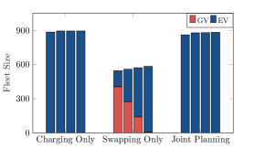
(a) Total Budget = 20

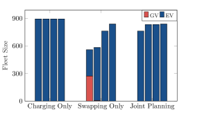
(b) Total Budget = 40

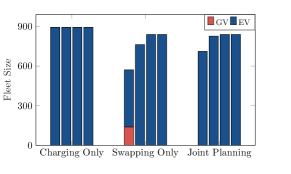
(c) Total Budget = 60

Figure 3: Fleet size and composition under varying budget levels. Each group consists of four bars, with each bar representing a different planning stage.

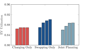
(a) Total Budget = 20

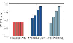
(b) Total Budget = 40

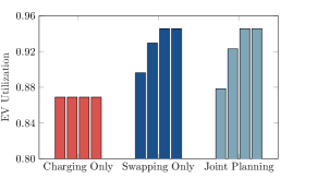
(c) Total Budget = 60

Figure 4: EV utilization under varying budget levels. Each group consists of four bars, with each bar representing a different planning stage.

To assess the performance of joint planning, we vary the total budget and compare different deployment strategies, including jointly deploying charging and battery swapping facilities versus deploying only one of them. The total profit gained from each strategy is illustrated in Figure 2. The results show that joint planning outperforms other deployment strategies in terms of profit maximization. For instance, with a total budget of 40 swapping stations, joint planning leads to a profit improvement of 4.06% and 2.91% when compared to charging-only and swapping-only strategies, respectively.

On the one hand, charging stations offer a cost-effective solution to support a large EV fleet under a tight budget. Figure 3 showcases the fleet size and composition at different planning stages under different budget levels. The results indicate that the platform can completely electrify the ride-hailing fleet from the first stage, even when the budget is limited. However, the long charging downtime poses an inherent bottleneck on EV utilization. As mentioned above, $(1-\epsilon)\Omega/\omega$ in (19) represents the battery range of an EV. The charging mode choice $r_{i,t}$ is fixed to 1 when only charging stations are deployed. If the number of charging stations goes to infinity, the time traveling to and waiting at each charging station is negligible. In this case, EV utilization becomes

$$\begin{split}\lim_{\tilde{x}^{c}\rightarrow\infty}\rho_{ev}&=1-\dfrac{\sum_{i=1}^{M}k_{i,t}\tau_{c}}{\sum_{i=1}^{M}N^{ve}_{i,t}+\sum_{i=1}^{M}\sum_{j=1}^{M}R_{i,t}\left(\lambda_{ij,t}w^{p}_{i,t}+\lambda_{ij,t}\tau_{ij}+f_{ij,t}\tau_{ij}\right)+\sum_{i=1}^{M}k_{i,t}\tau_{c}}\\ &=1-\dfrac{\tau_{c}\sum_{i=1}^{M}k_{i,t}}{\dfrac{(1-\epsilon)\Omega}{\omega}\sum_{i=1}^{M}k_{i,t}+\tau_{c}\sum_{i=1}^{M}k_{i,t}}\\ &=\dfrac{(1-\epsilon)\Omega/\omega}{(1-\epsilon)\Omega/\omega+\tau_{c}},\end{split}$$ (37)

where the second equality is derived by inserting (19) into (18b). This establishes a theoretical upper bound for EV utilization in the charging-only case. According to our simulation settings, $\lim_{\tilde{x}^{c}\rightarrow\infty}\rho_{ev}=88.89\%$. In other words, the EV fleet can be utilized at most 88.89% of its time, which underscores the bottleneck of plug-in charging associated with the long charging time. As a result, with a charging-only deployment strategy, the total profit only marginally improve as the total budget increases (see Figure 2). To further improve fleet utilization and the platform’s profit, it is crucial to consider complementary solutions such as battery swapping facilities or a hybrid charging infrastructure network.

On the other hand, battery swapping stations are expensive and difficult to scale, making the swapping-only deployment strategy insufficient for meeting the charging needs of a large EV fleet before the infrastructure network is extensively expanded. As shown in Figure 3, the platform has to downsize the fleet and adopt gasoline cars in the beginning when charging infrastructure is not yet sufficiently supplied, leading to a negative impact on profitability. The profit at each stage and the cumulative profit are presented in Figure 5-6, respectively. Due to the higher operational cost of gasoline cars, the swapping-only strategy results in a negative profit at the early stage and thus a longer pay-back period for the investment, especially under a limited budget. The total profit of swapping only is over 41% lower than that of joint planning when the budget is tight. However, under an ample budget, an extensive swapping station network can be built even at the early stage, enabling it to support a large EV fleet with much higher utilization than using plug-in charging, thereby yielding a higher total profit.

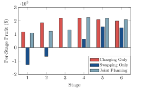
(a) Total Budget = 20

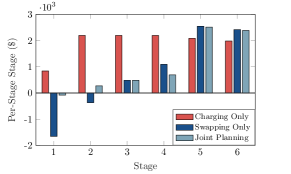
(b) Total Budget = 40

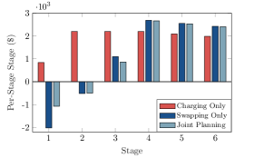
(c) Total Budget = 60

Figure 5: The platform’s profit at each stage under varying budget levels.

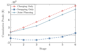
(a) Total Budget = 20

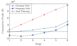
(b) Total Budget = 40

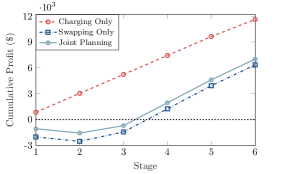
(c) Total Budget = 60

Figure 6: The platform’s cumulative profit under varying budget levels.

In contrast, joint planning combines the benefit of charging and battery swapping stations, thus eliciting the synergistic value between them. This strategy enables the platform not only to complete fleet electrification quickly by building charging stations at the early stage but also to overcome the bottleneck of plug-in charging and enhance fleet utilization by building battery swapping stations. As such, joint planning of the two facilities can yield a higher profit than deploying only one of them. Particularly, the deployment strategy and profit improvement depend on the budget level. The platform will only build charging stations when the budget is low and cannot support the deployment of battery swapping facilities, but will only consider battery swapping stations when the budget is generous enough to build an extensive network. Hence, the profit of joint planning is close to that of charging only under a tight budget but is close to that of swapping only under a sufficient budget.

5.4 Infrastructure Network Expansion

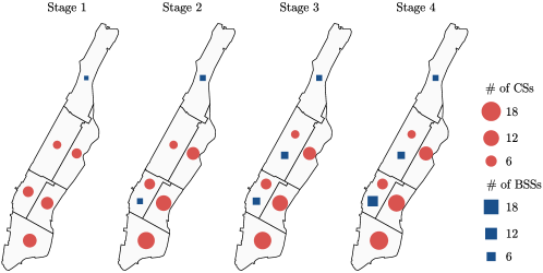
(a) Total Budget = 20

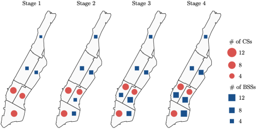
(b) Total Budget = 40

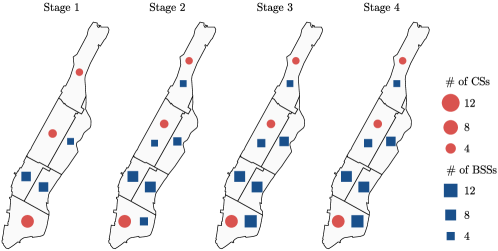
(c) Total Budget = 60

Figure 7: Infrastructure network expansion under different budget levels, with the red circles representing charging stations, the blue squares representing battery swapping stations, and their sizes representing the quantity of each type of facilities.

To further understand the benefits of joint planning, we present the expansion process of a mixed charging infrastructure network in Figure 7. For better visualization, we re-partition Manhattan into 6 zones, with the upper three zones corresponding to areas with lower passenger demand and the lower three zones corresponding to areas with higher passenger demand.

Interestingly, we find that charging and battery swapping stations play different roles at different stages of long-term infrastructure planning. Since the operational cost of EVs is much lower than gasoline vehicles, the platform prioritizes deploying charging stations at the early stage such that a dense charging network can be built to support fleet electrification. As investment increases, the bottleneck of plug-in charging becomes apparent, necessitating an upgrade of the infrastructure network. The platform then deploys battery swapping stations to enhance fleet utilization. The expansion process highlights the complementary effect between the two facilities, which again illustrates why joint planning is superior to other deployment strategies in profit maximization.

Another observation is that the deployment priority of battery swapping stations depends not only on passenger demand but also on budget levels. As the budget increases, priority is first given to low-demand zones and then shifts to high-demand ones. This is because charging demand is positively related to passenger demand in each zone. High-demand areas typically have high charging demand. When the budget is low, it can only cover a small number of battery swapping stations. Deploying these limited facilities in high-demand areas will force a large number of EVs to rely solely on a few battery swapping stations, resulting in congestion and low fleet utilization, which defeats the time-saving benefits of battery swapping. In contrast, low-demand areas generally have lower charging demand. A limited number of battery swapping stations can satisfy the demand without causing congestion. Therefore, under a tight budget, deployment priority is assigned to low-demand areas where charging demand is lower, so that congestion does not arise and the waiting time at battery swapping stations is under control. On the other hand, if the budget is generous enough to deploy many battery swapping stations, the platform prefers to first build these facilities in high-demand areas where more EVs could use battery swapping for recharge, so the economical benefit associated with quicker turnaround and improved fleet utilization can be fully utilized. These results shed light on how demand and budget levels will affect the optimal deployment strategy and thus can advise infrastructure planning.

6 Conclusion

This study investigates the planning of a multimodal charging network, where charging stations and battery swapping stations are jointly deployed to support an electric ride-hailing fleet. A multi-stage charging network expansion model is formulated to capture how the platform makes infrastructure planning and fleet operation decisions to maximize it profit. The model incorporates demand elasticity, charging and swapping congestion, stationary charging demand, and other fundamental components in an electrified ride-hailing market. A relaxed reformulation is developed to establish a theoretical upper bound for the nonconvex joint deployment problem. Moreover, We conduct a series of numerical studies to validate the proposed model using real data from Manhattan.

Our findings indicate that joint deployment can elicit synergistic value between the two facilities and generate a ”one plus one more than two” benefit. Compared to deploying only one of them, joint deployment not only enhances profitability and fleet utilization but also facilitates fleet electrification. At the early stage of infrastructure deployment, charging stations are prioritized to establish a dense network of charging stations that can electrify the entire fleet. As the investment budget increases, the platform starts building battery swapping stations to improve fleet utilization and maximize profit. These results confirm the effectiveness of the proposed multimodal charging network. We also briefly discuss the deployment priority of battery swapping stations and show that this priority is sensitive to passenger demand and investment budgets. Deployment of battery swapping infrastructure is initiated in high-demand areas under a generous budget but in low-demand areas under a limited budget.

This study opens up several research directions that await further investigation. For instance, we focus on market equilibrium in this work, whereas passenger demand varies over time in practice, and charging demand also changes accordingly. Therefore, a possible extension is to develop an adaptive charging mode choice strategy in response to the fluctuating charging demand so that the queuing delay in both facilities can be balanced. In addition, this paper considers a ride-hailing platform collaborates with infrastructure providers to deploy charging infrastructure and demonstrates the economical benefits of such partnership. While it remains unclear how these benefits would be divided between the two participants and how to ensure the stability of this partnership. These follow-up questions warrant further study. Moreover, future electric ride-hailing fleets could pose challenges and opportunities to urban power grids, especially considering the energy storage feature of battery swapping stations. So a dynamic charging and dispatching policy with integration of renewable energies is another interesting extension.

Appendix A Convexity of the Swapping Queue

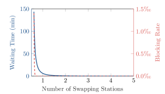
Figure 8: Waiting time and blocking rate in each swapping station

This section validates the convexity of the swapping queue (13)-(17) under a constant charging demand but varying infrastructure supply. The charging demand $k$ is fixed at $2.5\text{ veh/hr}$. Parameters in the queuing model include $t_{c},t_{s},W,C,B$ and $S$. We first test the queuing performance based on the nominal values. As shown in Figure 8, it is notable that the waiting time exhibits a convex relationship with respect to the number of facilities. For any facility density in a reasonable range where the waiting time at swapping stations is not too long (e.g., less than 1 hour), the blocking rate is negligible (e.g., below 0.05%), indicating that neglecting the blocking rate would not lead to a significant deviation at equilibrium.

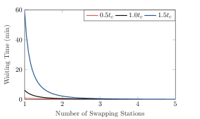
(a) Perturbing Charging Time

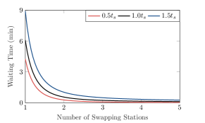
(b) Perturbing Swapping Time

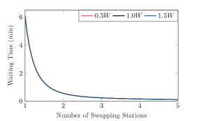
(c) Perturbing Queue Capacity

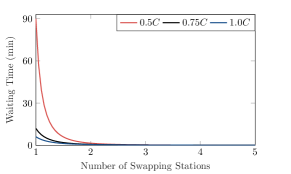
(d) Perturbing # of Chargers

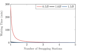
(e) Perturbing # of Batteries

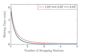
(f) Perturbing # of Swappers

Figure 9: Waiting time as a function the number of swapping stations under varying values of model parameters.

To further examine whether the convexity depends on model parameters, we perturb the parameters by 50% in both directions from their nominal values. The waiting time function under distinct values of model parameters is presented in Figure 9. We find that the convexity is robust to parameter variation. As the number of battery swapping station increases, waiting time reduces, and the marginal benefit of building additional facilities reduces as well. Particularly, waiting time is insensitive to the queue capacity in Figure 9c because a large nominal value is used to prevent the case of a full swapping queue. Although not analytically established, these results are sufficient to validate the convexity of the swapping queue under a wide range of model parameters, thereby confirming the applicability of the proposed approach.

References

- [1] Uber. Uber Q2 2022 Report, 2022. https://investor.uber.com/news-events/news/press-release-details/2022/Uber-Announces-Results-for-Second-Quarter-2022/default.aspx.
- [2] DiDi. DiDi’s Global Daily Trips Exceed 50 Million, 2020. https://www.didiglobal.com/news/newsDetail?id=955&type=news.
- [3] The Guardian. Electric cars account for under 5% of miles driven by Uber in Europe, 2021. https://www.theguardian.com/technology/2021/nov/03/electric-cars-under-5-per-cent-miles-driven-uber-europe.
- [4] Kelly L. Fleming and Mollie Cohen D’Agostino. Policy Pathways to TNC Electrification in California. Technical report, Institute of Transportation Studies, UC Davis, May 2020.
- [5] Alan Jenn. Emissions benefits of electric vehicles in Uber and Lyft ride-hailing services. Nature Energy, 5:520–525, July 2020.
- [6] Forbes. Uber, Lyft Have To Transition To Electric Vehicles In California, 2021. https://www.forbes.com/sites/alanohnsman/2021/05/20/uber-lyft-have-to-transition-to-electric-vehicles-under-new-california-rule/?sh=7214e57a6f20.
- [7] Uber. Together on the road to zero emissions. https://www.uber.com/us/en/drive/services/electric.
- [8] Lyft. Our commitment to achieve 100% electric vehicles across the lyft platform by 2030. https://www.lyft.com/impact/electric.
- [9] Angela Sanguinetti and Kenneth Kurani. Characteristics and Experiences of Ride-Hailing Drivers with Electric Vehicles. World Electric Vehicle Journal, 12(2):79, June 2021.
- [10] Zhichen Liu, Zhibin Chen, Yafeng Yin, and Zhengtian Xu. Regulatory policies to electrify ridesourcing systems. Transportation Research Part C: Emerging Technologies, 141:103743, August 2022.
- [11] Mohammad S. Roni, Zonggen Yi, and John G. Smart. Optimal charging management and infrastructure planning for free-floating shared electric vehicles. Transportation Research Part D: Transport and Environment, 76:155–175, November 2019.
- [12] Tesla. Supercharger. https://www.tesla.com/supercharger.
- [13] Jason Plautz. Shenzhen, china touts nearly all-electric taxi fleet. https://www.smartcitiesdive.com/news/electric-taxi-fleet-shenzhen-china/545347/.
- [14] Jiri Opletal. Geely launched Cao Cao 60 EV with swappable batteries and a 415 km range for $17,500. https://carnewschina.com/2023/03/30/geely-launched-cao-cao-60-ev-with-swappable-batteries-and-a-415-km-range-for-17500/.
- [15] South China Morning Post. China’s Didi Chuxing launches first electric vehicle tailored for ride-sharing services. https://www.scmp.com/tech/start-ups/article/3110132/chinas-didi-chuxing-launches-first-electric-vehicle-tailored-ride.
- [16] The Wall Street Journal. Uber Working With Auto Makers to Design EVs Customized for Ride-Sharing, Delivery. https://www.wsj.com/articles/uber-working-with-auto-makers-to-design-vehicles-customized-for-ride-sharing-delivery-11674132796.
- [17] CNBC. Uber to offer autonomous ride-hailing and delivery services using waymo’s robotaxis. https://www.cnbc.com/2023/05/23/uber-and-waymo-team-up-on-robotaxi-ride-hailing-and-delivery-services.html.
- [18] Reuters. China’s Didi Global to roll out self-developed robotaxis by 2025. https://www.reuters.com/business/autos-transportation/chinas-didi-global-roll-out-self-developed-robotaxis-by-2025-2023-04-13/.
- [19] ChinaDaily. Oil giant teams up with aulton to build battery swap stations. https://global.chinadaily.com.cn/a/202111/15/WS6191a703a310cdd39bc7548d.html.
- [20] Yingquan Li. The first batch of 12 battery swapping stations in guangzhou will be put into operation. https://www.stcn.com/article/detail/798359.html.
- [21] Ample. Accelerating the move to EVs. https://ample.com/fleets/#learn-about-ample.
- [22] Jintao Ke, Xuekai Cen, Hai Yang, Xiqun Chen, and Jieping Ye. Modelling drivers’ working and recharging schedules in a ride-sourcing market with electric vehicles and gasoline vehicles. Transportation Research Part E: Logistics and Transportation Review, 125:160–180, May 2019.
- [23] Xiaoran Qin, Kaixian Yu, Hanqian Li, Feng Dai, Haijiang Liu, Hai Yang, Jieping Ye, and Hongtu Zhu. Development of a one-day driving cycle for electric ride-hailing vehicles. Transportation Research Part D: Transport and Environment, 89:102597, December 2020.
- [24] Md Rakibul Alam, Chuang Hou, Spencer Aeschliman, Yan Zhou, and Zhaomiao Guo. Optimization-based trip chain emulation for electrified ride-sourcing charging demand analyses. Transportation Letters, 0(0):1–17, May 2022.
- [25] Jie Shi, Yuanqi Gao, Wei Wang, Nanpeng Yu, and Petros A. Ioannou. Operating Electric Vehicle Fleet for Ride-Hailing Services With Reinforcement Learning. IEEE Transactions on Intelligent Transportation Systems, 21(11):4822–4834, November 2020.
- [26] Nicholas D. Kullman, Martin Cousineau, Justin C. Goodson, and Jorge E. Mendoza. Dynamic Ride-Hailing with Electric Vehicles. Transportation Science, 56(3):775–794, May 2022.
- [27] Ji Hyun Hong and Xiaoxi Liu. The optimal pricing for green ride services in the ride-sharing economy. Transportation Research Part D: Transport and Environment, 104:103205, March 2022.
- [28] Yanyan Ding, Sen Li, and Sisi Jian. Optimal pricing and fleet management for shared electric vehicle in coupled power and transport networks. Transportation Research Part C: Emerging Technologies, 141:103727, August 2022.
- [29] Zeen Cai, Dong Mo, Maosi Geng, Wei Tang, and Xiqun Michael Chen. Integrating ride-sourcing with electric vehicle charging under mixed fleets and differentiated services. Transportation Research Part E: Logistics and Transportation Review, 169:102965, January 2023.
- [30] T. Donna Chen, Kara M. Kockelman, and Josiah P. Hanna. Operations of a shared, autonomous, electric vehicle fleet: Implications of vehicle & charging infrastructure decisions. Transportation Research Part A: Policy and Practice, 94:243–254, December 2016.
- [31] Berkay Turan, Ramtin Pedarsani, and Mahnoosh Alizadeh. Dynamic pricing and fleet management for electric autonomous mobility on demand systems. Transportation Research Part C: Emerging Technologies, 121:102829, December 2020.
- [32] Zonggen Yi and John Smart. A framework for integrated dispatching and charging management of an autonomous electric vehicle ride-hailing fleet. Transportation Research Part D: Transport and Environment, 95:102822, June 2021.
- [33] Lina Al-Kanj, Juliana Nascimento, and Warren B. Powell. Approximate dynamic programming for planning a ride-hailing system using autonomous fleets of electric vehicles. European Journal of Operational Research, 284(3):1088–1106, August 2020.
- [34] Peter Slowik, Sandra Wappelhorst, and Nicholas Lutsey. How can taxes and fees on ride-hailing fleets steer them to electrify? Technical report, International Council on Clean Transportation, 2019.
- [35] Dong Mo, Jingru Yu, and Xiqun Michael Chen. Modeling and managing heterogeneous ride-sourcing platforms with government subsidies on electric vehicles. Transportation Research Part B: Methodological, 139:447–472, September 2020.
- [36] Dale Hall, Mike Nicholas, and Marie Rajon Bernard. Guide to electrifying ride-hailing vehicles for cities. Working Paper, 2021.
- [37] Leah Lazer, Sadanand Wachche, Ryan Sclar, and Sarah Cassius. Electrifying Ride-Hailing in the United States, Europe, and Canada: How to Enable Ride-Hailing Drivers to Switch to Electric Vehicles. Technical report, World Resources Institute, 2021.
- [38] Zuo-Jun Max Shen, Bo Feng, Chao Mao, and Lun Ran. Optimization models for electric vehicle service operations: A literature review. Transportation Research Part B: Methodological, 128:462–477, October 2019.
- [39] Georg Brandstätter, Michael Kahr, and Markus Leitner. Determining optimal locations for charging stations of electric car-sharing systems under stochastic demand. Transportation Research Part B: Methodological, 104:17–35, October 2017.
- [40] Tai-Yu Ma and Simin Xie. Optimal fast charging station locations for electric ridesharing with vehicle-charging station assignment. Transportation Research Part D: Transport and Environment, 90:102682, January 2021.
- [41] Md Rakibul Alam and Zhaomiao Guo. Charging infrastructure planning for ride-sourcing electric vehicles considering drivers’ value of time. Transportation Letters, 0:1–11, May 2022.
- [42] Gordon S. Bauer, Amol Phadke, Jeffery B. Greenblatt, and Deepak Rajagopal. Electrifying urban ridesourcing fleets at no added cost through efficient use of charging infrastructure. Transportation Research Part C: Emerging Technologies, 105:385–404, August 2019.
- [43] Alan Jenn. Charging Forward: Deploying Electric Vehicle Infrastructure for Uber and Lyft in California. Technical report, UC Davis: Institute of Transportation Studies, 2021.
- [44] Ho-Yin Mak, Ying Rong, and Zuo-Jun Max Shen. Infrastructure Planning for Electric Vehicles with Battery Swapping. Management Science, 59(7):1557–1575, July 2013. Publisher: INFORMS.
- [45] Yang Wang, Wenjian Ding, Liusheng Huang, Zheng Wei, Hengchang Liu, and John A. Stankovic. Toward Urban Electric Taxi Systems in Smart Cities: The Battery Swapping Challenge. IEEE Transactions on Vehicular Technology, 67(3):1946–1960, March 2018.
- [46] William Infante, Jin Ma, Xiaoqing Han, and Ariel Liebman. Optimal Recourse Strategy for Battery Swapping Stations Considering Electric Vehicle Uncertainty. IEEE Transactions on Intelligent Transportation Systems, 21(4):1369–1379, April 2020.
- [47] Xiong Yang, Chunfu Shao, Chengxiang Zhuge, Mingdong Sun, Pinxi Wang, and Shiqi Wang. Deploying battery swap stations for shared electric vehicles using trajectory data. Transportation Research Part D: Transport and Environment, 97:102943, August 2021.
- [48] Joon Moon, Young Joo Kim, Taesu Cheong, and Sang Hwa Song. Locating Battery Swapping Stations for a Smart e-Bus System. Sustainability, 12(3):1142, January 2020.
- [49] BP. BP and DiDi join forces to build electric vehicle charging network in China. https://www.bp.com/en/global/corporate/news-and-insights/press-releases/bp-and-didi-join-forces-to-build-electric-vehicle-charging-network-in-china.html.
- [50] Buesinesswire. Uber and Wallbox to expand partnership to all of the U.S. https://www.businesswire.com/news/home/20220201005729/en/Uber-and-Wallbox-to-Expand-Partnership-to-All-of-The-U.S.
- [51] Ample. Announcing a New Ride Sharing EV Experience with Sally. https://ample.com/2021/06/10/announcing-a-new-ride-sharing-ev-experience-with-sally/.
- [52] Zeyi Yang. China plans charging infrastructure for 20 million EVs. https://www.protocol.com/bulletins/china-infrastructure-plan-ev.
- [53] EVbox. Ev charging infrastructure incentives in Europe 2022. https://blog.evbox.com/ev-charging-infrastructure-incentives-eu#:~:text=A%2045%20percent%20personal%20income,charging%20point%20and%20per%20taxpayer.
- [54] Yaqian Zhou, Hai Yang, Jintao Ke, Hai Wang, and Xinwei Li. Competition and third-party platform-integration in ride-sourcing markets. Transportation Research Part B: Methodological, 159:76–103, May 2022.
- [55] Richard Arnott. Taxi travel should be subsidized. Journal of Urban Economics, 40(3):316–333, 1996.
- [56] Sen Li, Hamidreza Tavafoghi, Kameshwar Poolla, and Pravin Varaiya. Regulating TNCs: Should Uber and Lyft set their own rules? Transportation Research Part B: Methodological, 129:193–225, November 2019.
- [57] Juan Camilo Castillo, Dan Knoepfle, and Glen Weyl. Surge pricing solves the wild goose chase. In Proceedings of the 2017 ACM Conference on Economics and Computation, page 241–242, 2017.
- [58] Jintao Ke, Hai Yang, Xinwei Li, Hai Wang, and Jieping Ye. Pricing and equilibrium in on-demand ride-pooling markets. Transportation Research Part B: Methodological, 139:411–431, 2020.
- [59] Xinwu Qian, Jiawei Xue, Stanislav Sobolevsky, Chao Yang, and Satish Ukkusuri. Stationary Spatial Charging Demand Distribution for Commercial Electric Vehicles in Urban Area. In 2019 IEEE Intelligent Transportation Systems Conference (ITSC), pages 220–225, October 2019.
- [60] Gilbert Strang. Introduction to Linear Algebra, volume 3. Wellesley-Cambridge Press, 1993.
- [61] Yongjun Ahn and Hwasoo Yeo. An Analytical Planning Model to Estimate the Optimal Density of Charging Stations for Electric Vehicles. PloS one, 10(11):e0141307, November 2015.
- [62] Frederick S. Hillier and Gerald J. Lieberman. Introduction to Operations Research. McGraw-Hill Higher Education, July 2004.
- [63] Xiaoqi Tan, Bo Sun, and Danny H. K. Tsang. Queueing network models for electric vehicle charging station with battery swapping. In 2014 IEEE International Conference on Smart Grid Communications (SmartGridComm), pages 1–6, November 2014.
- [64] Dimitri Bertsekas. Nonlinear Programming. Athena Scientific, 3rd edition, 2016.
- [65] M. E. Dyer and L. G. Proll. On the validity of marginal analysis for allocating servers in m/m/c queues. Management Science, 23(9):1019–1022, 1977.
- [66] TLC Trip Record Data - TLC. https://www1.nyc.gov/site/tlc/about/tlc-trip-record-data.page.
- [67] Tian Lei, Shuocheng Guo, Xinwu Qian, and Lei Gong. Understanding charging dynamics of fully-electrified taxi services using large-scale trajectory data. Transportation Research Part C: Emerging Technologies, 143:103822, 2022.