Iterative regularization in classification via hinge loss diagonal descent

Abstract

Iterative regularization is a classic idea in regularization theory, that has recently become popular in machine learning. On the one hand, it allows to design efficient algorithms controlling at the same time numerical and statistical accuracy. On the other hand it allows to shed light on the learning curves observed while training neural networks. In this paper, we focus on iterative regularization in the context of classification. After contrasting this setting with that of regression and inverse problems, we develop an iterative regularization approach based on the use of the hinge loss function. More precisely we consider a diagonal approach for a family of algorithms for which we prove convergence as well as rates of convergence. Our approach compares favorably with other alternatives, as confirmed also in numerical simulations.

1 Introduction

Estimating a quantity of interest from finite measurements is a central problem in a number of fields including machine learning but also statistics and signal processing. In this context, a key idea is that reliable estimation requires imposing some prior assumptions on the problem at hand. The theory of inverse problems provides a principled framework to formalize this idea [27]. The quantity of interest is typically seen as a function, or a vector, and prior assumptions take the form of suitable functionals, called regularizers. Following this idea, Tikhonov regularization provides a classic approach to estimate solutions [83, 84]. Indeed, the latter are found by minimizing an empirical objective where a data fit term is penalized adding the chosen regularizer. Other regularization approaches are classic in inverse problems, and in particular iterative regularization has become popular in machine learning, see e.g. [86, 70, 80]. This approach is based on the observation that iterative optimization procedures have a self-regularizing property, so that a chosen prior is enforced along the iterations. Such an observation seems to shed light on some theoretical properties of deep learning approaches [37, 61, 33, 34, 69]. More generally, it provides an approach to design algorithms striking a balance between statistical accuracy and computational efficiency [13, 89, 71, 53].

In this paper, we focus on iterative regularization in the context of classification, perhaps the most classical among machine learning problems [23, 81, 77]. After discussing the differences and similarities between classification and regression, we recall how different iterative regularization schemes for classification can be defined depending on the considered loss function. Then, we focus on the hinge loss used in support vector machines [81]. In this case, compared to other loss functions such as the exponential and logistic loss [58, 79, 42], a simple gradient approach does not allow to establish iterative regularization properties. Indeed, towards this end, we propose a diagonal approach in the same spirit of [31] and its inertial version [17] and prove their regularization properties, including convergence rates. The proposed approach compares favorably to analogous results for the logistic loss [58, 79, 42, 40], but also with recent similar approaches considering the hinge loss [55]. Indeed, we show that linear convergence is possible hence providing substantial improvements over previous studies yielding only sub-linear rates. Beyond a regularization perspective, our approach can also be seen as a way to solve the basic separable support vector machines problem introduced in the seminal work [23]. In this view, relevant studies, among the rich literature, can be found for example in [23, 29, 24, 19, 78]. Our theoretical results are illustrated via numerical simulations, where we also investigate empirically the stability properties of the proposed methods.

The rest of the paper is organized as follows. In Section 2, we briefly discuss the ideas of explicit and implicit regularization approach for regression problems. In Section 3 we are reviewing these approaches in terms of classification problems. In Section 4, we describe the main proposed schemes based on a diagonal iterative regularization procedure for the hinge loss. In Section 5 we present the main results and we provide the corresponding convergence analysis. Finally in Section 6 we illustrate the performance of the proposed algorithms on some simple numerical examples. Appendix A contains some general facts and most of the technical proofs and lemmas needed in the main core of the paper.

1.1 Notation

We first introduce some notations and recall a few basic notions that will be needed throughout the paper. The interested reader can consult [9] regarding the main tools and their associated properties used in this work. Let $\left\langle{\cdot},{\cdot}\right\rangle$ denote the standard Euclidean inner product and $\left\lVert{\cdot}\right\rVert$ the associated Euclidean norm. For a linear operator $Z:\mathbb{R}^{n}\to\mathbb{R}^{m}$, we denote with $\Im(Z)$ and $\ker(Z)$ its range and kernel respectively We also note with $\left\lVert{Z}\right\rVert_{op}$ and $\left\lVert{Z}\right\rVert_{F}$ its operator and Frobenious norm respectively. We also denote with Id the identity operator and with $\mathbf{1}$ the $n$-vector with entry $1$ in each coordinate.

Given a convex and closed set $C\subset\mathbb{R}^{n}$, the distance of a point $x\in\mathbb{R}^{n}$ from the set $C$ is $\text{dist}(x,C)=\underset{y\in C}{\inf}\left\lVert{x-y}\right\rVert$. The indicator function of $C$, $\iota_{C}(\cdot):\mathbb{R}^{n}\to\bar{\mathbb{R}}:=\mathbb{R}\cup\{+\infty\}$ is defined as $\iota_{C}(x)=\begin{cases}&0~{}\text{ if }x\in C\\ &+\infty~{}\text{ if not }\end{cases}.$

For a proper, convex and lower semicontinuous function $f:\mathbb{R}^{n}\to\bar{\mathbb{R}}$, we define its subdifferential $\partial f:\mathbb{R}^{n}\to 2^{\mathbb{R}^{n}}$, as $\partial f(x)=\{u\in\mathbb{R}^{n}~{}:~{}f(y)\geq f(x)+\left\langle{u},{y-x}\right\rangle,~{}\forall y\in\mathbb{R}^{n}\}$. For $\gamma>0$, the proximal operator of $f$, $\operatorname{prox}_{\gamma f}:\mathbb{R}^{n}\to\mathbb{R}^{n}$ with step $\gamma$, is defined by $\operatorname{prox}_{\gamma f}(x)=\underset{y\in\mathbb{R}^{n}}{\operatornamewithlimits{arg\,min}}\{f(y)+\frac{1}{2\gamma}\left\lVert{x-y}\right\rVert^{2}\}$, for all $x\in\mathbb{R}^{n}$. The projection operator onto a convex and closed set $C\subset\mathbb{R}^{n}$ is defined as $\operatorname{proj}_{C}:\mathbb{R}^{n}\to\mathbb{R}^{n}$ such that $\operatorname{proj}_{C}(x)=\underset{y\in C}{\operatornamewithlimits{arg\,min}}\left\lVert{y-x}\right\rVert$. We denote the Fenchel conjugate of $f$ as $f^{\ast}:\mathbb{R}^{n}\to\bar{\mathbb{R}}$, such that $f^{\ast}(x)=\underset{y\in\mathbb{R}^{n}}{\sup}\{\left\langle{x},{y}\right\rangle-f(y)\}$.

2 Background: explicit and implicit regularization in regression

The classical regression problem in supervised learning and statistics corresponds to estimating a function of interest $f$ , given a finite number of (possibly noisy) evaluations at a number of input points. The problem takes a simple and familiar form if $f$ is assumed to be linear. Indeed, in this case it corresponds to estimating $w\in\mathbb{R}^{d}$, given a set of equations,

$$\left\langle{w},{x_{i}}\right\rangle=y_{i},\qquad i=1,\dots,n,$$ (2.1)

where $x_{i}\in\mathbb{R}^{d}$ and $y_{i}\in\mathbb{R}$.

The above problem can be restated as the linear equation

$$Xw=y,$$ (2.2)

where $X:\mathbb{R}^{d}\to\mathbb{R}^{n}$ is a matrix with rows the input points, and $y\in\mathbb{R}^{n}$ is a vector with entries the outputs. Moreover, the simple linear case can be generalized if $f$ belongs to a reproducing kernel Hilbert space (RKHS).

Remark 2.1 (Regression in RKHS [81]).

Recall that a Hilbert space $\mathcal{H}$ of real valued functions on a set $\cal X$ is called a RKHS if for all $f\in\mathcal{H}$ and $x\in\cal X$, there exists $C_{x}\in\mathbb{R}$ such that $|f(x)|\leq C_{x}\left\lVert{f}\right\rVert_{\mathcal{H}}.$ From the above definition and Riesz lemma it follows immediately that there exists a $k_{x}\in\mathcal{H}$ such that $f(x)=\left\langle{f},{k_{x}}\right\rangle_{\mathcal{H}}.$ Then we can write the regression problem as the problem of finding $f\in\mathcal{H}$, given a set of equations,

$$\left\langle{f},{k_{x_{i}}}\right\rangle_{\mathcal{H}}=y_{i},\qquad i=1,\dots,n,$$

where $x_{i}\in\cal X$ and $y_{i}\in\mathbb{R}$.

Keeping the above remark in mind, in the following we primarily focus on the linear case to ease the notation.

A key observation is that the problem (2.1) might not admit solutions or admit multiple ones. This latter situation is the most common one in machine learning, where high dimensional (overparameterized), or even infinite dimensional (like RKHS) models are often considered. In the linear setting, this corresponds to the case where $n<d$ in (2.1), (assuming the inputs to be linearly independent). In this case, problem (2.1) admits infinitely many solutions and a classic way to select one is to consider the minimum norm solution

$$w^{\dagger}=\operatornamewithlimits{arg\,min}_{w\in\mathbb{R}^{d}}\big{\{}\left\lVert{w}\right\rVert~{}:~{}\left\langle{w},{x_{i}}\right\rangle=y_{i},\quad i=1,\dots,n\big{\}}.$$ (2.3)

The minimum norm solution can be written in terms of the pseudoinverse of $X$ as $w^{\dagger}=X^{\dagger}y$ [27, Definition $2.2$]. This makes it clear that instability in the solution might occur when $X$ is ill conditioned. The basic idea of regularization is to consider a family of solutions with better stability properties. In particular a family of solutions is said to have the regularization property if it converges to the minimal norm solution (see e.g. [27, Section $2$]). We next recall two basic approaches with this property.

Tikhonov (explicit) regularization.

The most classic regularization approach is Tikhonov regularization

$$w_{\lambda}=\operatornamewithlimits{arg\,min}_{w\in R^{d}}\sum_{i=1}^{n}(y_{i}-\left\langle{w},{x_{i}}\right\rangle)^{2}+\lambda\left\lVert{w}\right\rVert^{2},$$ (2.4)

where $\lambda>0$ is called the regularization parameter. The set of solutions corresponding to different values of $\lambda$ defines the regularization method and a direct computation shows that $w_{\lambda}=(X^{\top}X+\lambda\text{Id})^{-1}X^{\top}y$. From this expression is easy to see that the sequence $w_{\lambda}$ converges to $w^{\dagger}$ as $\lambda$ tends to zero, showing the regularization property of the method (see e.g. [27, Theorem $5.2$]). The above ideas can be generalized as we discuss next.

Remark 2.2 (Loss and regularizers).

The ideas in (2.3), (2.4) can be generalized replacing the squared norm in (2.4) with other regularizers $R:\mathbb{R}^{d}\to[0,\infty)$, the $\ell_{1}$ norm being a popular example. Similarly instead of the least squares error in (2.4) other error cost functions (loss functions) $\ell:\mathbb{R}\to[0,\infty)$ can be considered. In regression, loss functions depend on the difference $y-f(x)$, examples besides the square loss include the absolute value loss, or the $epsilon$-insensitive loss used in support vector machine regression [81]. For general losses, the corresponding solutions might not admit a closed form expression, but it is still possible to prove that the Tikhonov regularized solutions converge in some proper sense to the corresponding minimum norm solutions (see e.g. [26, 4]). For sake of completeness we provide a proof in a general setting in Lemma A.1 in Appendix A.

In machine learning, regularization à la Tikhonov is sometimes called explicit since a penalty is added to the data fit term. We next recall iterative regularization and discuss why it is called implicit in machine learning [36].

Iterative (implicit) regularization.

The simplest example of iterative regularization is the gradient descent iteration of the least squares error, that is

$$w_{t+1}=w_{t}-\gamma\sum_{i=1}^{n}x_{i}(y_{i}-\left\langle{w_{t}},{x_{i}}\right\rangle),\quad t=0,\dots,T.$$

for some suitable initialization $w_{0}$ and step size $\gamma$. It is well known that the above iteration converges to the minimal norm solution (2.3), and further that the stability of the solution varies along the iterations [27, Section $6.1$]. In this view, the stopping time becomes the regularization parameter defining a family of regularized solutions. This kind of regularization is called implicit in machine learning since there is no explicit penalty or constraint in the optimization model [62, 61]. These ideas have recently received a lot of attention, since they are useful to understand the theoretical properties of more complex non-linear systems like neural networks [36, 20]. Further, they have been advocated as a way to design resource efficient machine learning algorithms controlling at the same time numerical and statistical accuracy. In the remainder of the paper we discuss how these ideas extend beyond regression to the classification setting.

We first add some remarks. First, we note that other optimization approaches than gradient descent can be, and have been considered, including accelerated [27, 60, 64] and stochastic methods [72, 56, 25], as also mirror descent approaches [35]. Second we note that, compared to Tikhonov regularization, for iterative regularization the extension to other losses and regularizers is not straightforward. The case of regularizers that are norms in reflexive Banach space has been considered in [76, 16], whereas the case of strongly convex regularizers has been considered in [53, 33]. The case of convex regularizers has been recently considered in [54]. The case of smooth loss functions for regression is quite straightforward, considering the gradient iteration

$$w_{t+1}=w_{t}-\gamma\sum_{i=1}^{n}x_{i}\ell^{\prime}(y_{i}-\left\langle{w_{t}},{x_{i}}\right\rangle),\quad t=0,\dots,T,$$ (2.5)

where $\ell^{\prime}$ is the derivative of the loss. The case of convex but non smooth loss function can also be considered using subgradient methods [47]. Note that, if the above iteration is initialized in the span of the input points, it remains in the span. This observation is at basis of the proof that the above iteration converges to the minimal norm interpolant (2.3), see Lemma A.2 in Appendix A.

Provided, with the above background we next discuss the case of classification.

3 Implicit regularization: from regression to classification

In this section, we introduce the problem of classification and investigate how the ideas introduced in the previous section for regression translate to this setting. In particular, we first discuss a corresponding notion of minimal norm solution.

Similarly to regression, in classification the goal is to estimate a functional relationship, but the difference is that the outputs are binary valued, that is $y_{i}\in\{-1,1\}$. Estimating a binary valued function is computationally cumbsersome and the classic approach relies on estimating a real valued function $f$ of which the sign is then taken, that is $\text{sign}(f(x))=1$ if $f(x)>0$, and $\text{sign}(f(x))=-1$ otherwise (here ties are broken arbitrarily). In this context, a natural quantity is the product $yf(x)$, called the margin of $f$ at $(x,y)$. If the margin is positive it means that $f$ will classify correctly the input point, if the margin is large we can intuitively expect a confident prediction.

For linear functions we can formalize this idea (see e.g. [23, 81]) considering the problem of finding $w\in\mathbb{R}^{d}$ satisfying the set of inequalities

$$y_{i}\left\langle{w},{x_{i}}\right\rangle>0,\quad i=1,\dots,n.$$ (3.1)

If such a $w$ exists we say that the data $(x_{1},y_{1}),\dots,(x_{n},y_{n})$ are linearly separable. Deriving necessary and sufficient conditions for the above inequalities to be feasible is not an elementary problem. As shown below, it is easy to see that overparametrization ($n<d$), hence interpolation, will be a sufficient condition for linear separability. Since this is the relevant setting for us, from now on, we assume that the data are linearly separable:

Assumption 1 (Linear separability).

There exists some $\tilde{w}\in\mathbb{R}^{d}$ that separates the data, i.e.

$$y_{i}\left\langle{\tilde{w}},{x_{i}}\right\rangle>0\qquad\forall i=1,...,n$$ (3.2)

In general, also in this setting we can expect multiple solutions, the classical way to approach the problem is to consider the so called max margin solution. The linear margin $M:\mathbb{R}^{d}\to\mathbb{R}$ for a given dataset is defined as,

$$M(w)=\min_{i=1,\dots,n}y_{i}\left\langle{w},{x_{i}}\right\rangle,$$ (3.3)

and, correspondingly, the maximum (max) margin problem is defined as

$$w_{+}=\operatornamewithlimits{arg\,max}\{M(w)~{}:~{}\left\lVert{w}\right\rVert=1\}.$$ (MM)

We make a few observations. First, the intuition underling the above problem is that among all separating solutions, we are interested into one for which the margin is maximized. Second, we note that without the unit norm constraint the problem of maximizing the margin (3.3) is degenerate and one can obtain trivial solutions by rescaling arbitrarily any separating solution. Indeed since the margin is scale invariant, the max margin becomes a direction problem, which naturally leads to considering the constrained problem (MM). Third, it is possible to show that the max margin problem has an equivalent formulation, that highlights the connection to minimal norm solutions. Indeed, consider the problem

$$w_{\ast}=\operatornamewithlimits{arg\,min}_{w\in\mathbb{R}^{d}}\big{\{}\left\lVert{w}\right\rVert~{}:~{}y_{i}\left\langle{w},{x_{i}}\right\rangle\geq 1~{},~{}\forall i\leq n\big{\}}.$$ (MN)

Then the following result holds.

Lemma 3.1.

Problem (MM) is equivalent to Problem (MN). In particular, if $w_{\ast}$ is a solution of Problem (MN) then

$$w_{+}=\frac{w_{\ast}}{\left\lVert{w_{\ast}}\right\rVert}$$

is a solution of Problem (MM) and $M(w_{+})=\frac{1}{\left\lVert{w_{\ast}}\right\rVert}$. Moreover, if $w_{+}$ is the solution of Problem (MM) then

$$w_{\ast}=\frac{w_{+}}{M(w_{+})}$$

is a solution of Problem (MN). Further, it holds that $M(w_{\ast})=1$

A few observations can be made. The above lemma is a classical result in the theory of SVM. Indeed, Problem (MN) defines the hard margin support vector machines algorithm [23]. For sake of completeness we provide its proof (see Lemma A.3 in Appendix A). In terms of the constrained min-norm problem (MN), Assumption 1, ensures that the feasible set is non-empty and hence such a solution $w_{\ast}$ (thus $w_{+}$) exists. In addition since (MN) can also be equivalently expressed as

$$w_{\ast}=\operatornamewithlimits{arg\,min}_{w\in\mathbb{R}^{d}}\left\{\frac{\left\lVert{w}\right\rVert^{2}}{2}~{}:~{}y_{i}\left\langle{w},{x_{i}}\right\rangle\geq 1~{},~{}\forall i\leq n\right\},$$ (3.4)

the solution $w_{\ast}$ (thus $w_{+}$) is unique, thanks to the strong convexity of the squared norm in (3.4). Notice that from an optimization point of view, formulation (3.4) is more useful and will be used hereafter, instead of (MN).

From the regularization perspective taken thus far, the above result shows that the max margin problem can identified as the minimum norm problem akin to Problem (2.3) in regression, but the linear equations are now replaced by inequalities. This can be made even more explicit noting that for binary valued outputs, it holds:

$$y_{i}=\left\langle{w},{x_{i}}\right\rangle~{}\Leftrightarrow~{}y_{i}\left\langle{w},{x_{i}}\right\rangle=1$$

This last expression also clarifies the earlier observation that interpolation implies separation, and that $n<d$ with linearly independent inputs is a sufficient condition for linear separability.

We next discuss how the ideas of explicit and implicit regularization can be adapted to the classification context. Note that in the following, in analogy to the regression case, we will say that a family of solutions has the regularization property if it converges to the max margin (min norm) solution.

Explicit regularization for classification.

To extend Tikhonov regularization approach to classification, an appropriate loss function $\ell:\mathbb{R}\to[0,\infty)$ needs to be considered. As it turns out in classification, loss functions depend on the margin $yf(x)$, rather than the difference $y-f(x)$ as in regression, and indeed are called margin loss functions. Some popular examples are the following:

• hinge loss :   $\ell(a)=\lvert{1-a}\rvert_{+}=\max\{0,1-a\}$

• exponential loss :  $\ell(a)=e^{-a}$

• logistic loss :  $\ell(a)=\ln(1+e^{-a})$

Figure 1: The exponential (blue), logistic (red) and hinge (green) loss function.

Given a convex margin loss function, and considering again linear models, Tikhonov regularization in classification corresponds to

$$w_{\lambda}=\operatornamewithlimits{arg\,min}_{w\in R^{d}}\sum_{i=1}^{n}\ell(y_{i}\left\langle{w},{x_{i}}\right\rangle)+\lambda\left\lVert{w}\right\rVert^{2},$$ (3.5)

for $\lambda>0$. It is natural to ask whether the above approach can be shown to be regularizing in the sense that the sequence $\{w_{\lambda}\}_{\lambda>0}$ converges to the minimum norm solution (MN). Indeed, for the hinge loss this can be proven, while in the cases of the exponential or logistic loss, where the set of minimizers is empty, one can show that $w_{\lambda}$ diverges (see e.g. Lemma A.1 in Appendix A). Nevertheless under some suitable assumptions on the loss function, convergence in direction that is

$$\frac{w_{\lambda}}{\left\lVert{w_{\lambda}}\right\rVert}\underset{\lambda\to 0}{\to}\frac{w_{\ast}}{\left\lVert{w_{\ast}}\right\rVert}=w_{+}$$

has been proven for a wide class of margin loss functions (see e.g. [74, Theorem $2.1$] and [38, 73]). Notice that according to the previous discussion and Lemma 3.1, since the max margin problem (MM) is a direction problem, it is still relevant to consider convergence in direction. We next turn our attention to implicit regularization reviewing some recent results.

Implicit regularization for classification.

Following the same reasoning as in regression for the minimal norm interpolating solution (2.3) and the gradient method (2.5), it is natural to ask whether it is possible to prove the regularization properties of the gradient iteration applied to a margin loss function, i.e.

$$w_{t+1}=w_{t}-\gamma\sum_{i=1}^{n}y_{i}x_{i}\ell^{\prime}(y_{i}\left\langle{w_{t}},{x_{i}}\right\rangle),\quad t=0,\dots,T.$$ (3.6)

where $\gamma>0$ is a suitable step size. The above iteration is well defined for smooth loss functions such as the exponential or the logistic loss. However, for losses like exponential or logistic which do not admit any minimizer, the gradient descent iteration in (3.6) diverges. Interestingly, in a recent line of works (see [79, 58, 42] and references therein), convergence in direction of gradient descent has been proved for these loss functions, i.e.

$$\lim_{t\to\infty}\frac{w_{t}}{\left\lVert{w_{t}}\right\rVert}=w_{+}.$$

In addition, rates of convergence for the normalized iterates $\left\lVert{\frac{w_{t}}{\left\lVert{w_{t}}\right\rVert}-w_{+}}\right\rVert$, as also for the angle gap, that is $1-\left\langle{\frac{w_{t}}{\left\lVert{w_{t}}\right\rVert}},{w_{+}}\right\rangle$, and the normalized margin gap $M\left(\frac{w_{t}}{\left\lVert{w_{t}}\right\rVert}\right)-M(w_{+})$ were also proved but are very slow. For example for the logistic and exponential losses the margin rate is of order $O\mathopen{}\left(\frac{1}{\log t}\right)$ (see [79]). Improved rates of order $O\mathopen{}\left(\frac{\log t}{\sqrt{t}}\right)$ were given recently considering a variable step-size gradient descent version in [58]. Similar works include also (accelerated) mirror descent approaches [40, 41] that provide margin rates up to $O\mathopen{}\left(\frac{\log t}{t^{2}}\right)$. Concerning the hinge loss, the natural extension of the above idea is to consider a subgradient iteration

$$w_{t+1}=w_{t}-\gamma_{t}\sum_{i=1}^{n}y_{i}x_{i}g_{i}(w_{t}),\quad t=0,\dots,T.$$ (3.7)

for some sequence of step-sizes $(\gamma_{t})_{t}$ and where $g_{i}(w_{t})\in\partial\ell(y_{i}\left\langle{w_{t}},{x_{i}}\right\rangle)$ is an element of the subgradient of the loss. In this case, the minimization problem

$$\min_{w\in\mathbb{R}^{d}}\sum_{i=1}^{n}|1-y_{i}\left\langle{w_{t}},{x_{i}}\right\rangle|_{+}$$

does have a solution and indeed the iteration in (3.7) converges to it. However, the solution minimizing the hinge loss error cannot be expected to be a max margin (min norm) solution in general, and thus the subgradient iteration in (3.7) does not have the regularization property, as in the regression setting.

In this work we focus on the case of the hinge loss and provide two iterative regularization schemes via a diagonal principle. For ease of reading, we first present and describe the two main iterative methods and then the main convergence results.

4 Iterative regularization for hinge loss via diagonal descent

In this section, we present the two procedures we propose and study to derive efficient iterative regularization approaches based on the hinge loss. The first is given in Algorithm 1, while the second one is Algorithm 2 and corresponds to a potentially faster variant.

Algorithm 1 Projected iterative GD on the dual

Let $\{\lambda_{t}\}_{t\geq 0}$ be a decreasing-to-zero sequence of positive numbers, $u_{0}\in[-\lambda_{0}^{-1},0]^{n}$ and $0<\gamma\leq\left\lVert{XX^{\top}}\right\rVert_{\text{op}}^{-1}$. For all $t\geq 0$, consider $g_{t}=(g_{t}^{i})_{i=1,...,n}$, $u_{t}=(u_{t}^{i})_{i=1,...,n}$ and $w_{t}=(w_{t}^{i})_{i=1,...,n}$, such that for all $i=1,...,n$ :

$$g_{t}^{i} =u_{t}^{i}-\gamma\sum_{j=1}^{n}y_{i}y_{j}\left\langle{x_{i}},{x_{j}}\right\rangle u_{t}^{j}$$ (4.1)

$$u_{t+1}^{i} =\begin{cases}-\frac{1}{\lambda_{t}}&\text{ if }g_{t}^{i}<\gamma-\frac{1}{\lambda_{t}}\\ g_{t}^{i}-\gamma&\text{ if }g_{t}^{i}\in[\gamma-\frac{1}{\lambda_{t}},\gamma]\\ 0&\text{ if }g_{t}^{i}>\gamma\end{cases}$$ (4.2)

$$w_{t+1}^{i} =-\sum_{i=1}^{n}y_{i}\left\langle{x_{i}},{u_{t+1}^{i}}\right\rangle$$ (4.3)

Algorithm 2 Projected iterative i-GD on the dual

Let $\{\lambda_{t}\}_{t\geq 0}$ a decreasing-to-zero sequence of positive numbers, $u_{0}=u_{1}\in[-\lambda_{0}^{-1},0]^{n}$ and $0<\gamma\leq\left\lVert{XX^{\top}}\right\rVert_{\text{op}}^{-1}$. For all $t\geq 1$, consider $z_{t}=(z_{t}^{i})_{i=1,...,n}$, $g_{t}=(g_{t}^{i})_{i=1,...,n}$, $u_{t}=(u_{t}^{i})_{i=1,...,n}$ and $w_{t}=(w_{t}^{i})_{i=1,...,n}$, such that for all $i=1,...,n$ :

$$z_{t}^{i} =u_{t}^{i}+\alpha_{t}(u_{t}^{i}-u_{t-1}^{i})\quad,\quad\alpha_{t}=\frac{t}{t+\alpha}$$ (4.4)

$$g_{t}^{i} =z_{t}^{i}-\gamma\sum_{j=1}^{n}y_{i}y_{j}\left\langle{x_{i}},{x_{j}}\right\rangle z_{t}^{j}$$ (4.5)

$$u_{t+1}^{i} =\begin{cases}-\frac{1}{\lambda_{t}}&\text{ if }g_{t}^{i}<\gamma-\frac{1}{\lambda_{t}}\\ g_{t}^{i}-\gamma&\text{ if }g_{t}^{i}\in[\gamma-\frac{1}{\lambda_{t}},\gamma]\\ 0&\text{ if }g_{t}^{i}>\gamma\end{cases}$$ (4.6)

$$w_{t+1}^{i} =-\sum_{i=1}^{n}y_{i}\left\langle{x_{i}},{u_{t+1}^{i}}\right\rangle$$ (4.7)

We add a few comments before providing a detailed derivation of the two procedures above. In both algorithms 1 and 2, $\gamma$ denotes the step-size and $\lambda_{t}$ a vanishing-with-iterations regularization parameter. Both procedures are based on simple and easy to implement iterations that require only vector multiplication and thresholding operations. The sequence $\{u_{t}\}_{t\geq 0}$ represents a dual variable and is computed coordinate-wise via a simple projection operation (see (4.2) and (4.6)), while $g_{t}$ corresponds to a classical gradient (forward) step related to the square norm ${\left\lVert{\cdot}\right\rVert^{2}}/{2}$. We note that the difference between the two schemes is that in Algorithm 2 the sequence $g_{t}$ is computed via the auxiliary sequence $z_{t}$ instead of $u_{t}$. The sequence $z_{t}$ equals to $u_{t}$ extrapolated by the term $\alpha_{t}(u_{t}-u_{t-1})$, called inertial term, which plays an important role on the convergence speed of Algorithm 2. Finally, $\{w_{t}\}_{t>0}$ corresponds to the primal sequence designed to approximate the min-norm solution $w_{\ast}$. In the next section, we discuss the derivation of the above two procedures.

4.1 Diagonal methods via dual hinge loss

Algorithms 1 and 2 are based on a so called diagonal regularization process [8] applied to a suitably defined dual problem. We next describe these ideas in some detail. We note in passing that, while diagonal approaches have been considered before for inverse problems [7, 52, 15, 8, 31, 17]), we are not aware of their application to classification.

The basic idea of diagonal approaches can perhaps be better explained recalling that the penalized functional such as (3.5) converges to minimal norm separating solution (3.4), as the regularization parameter goes to zero. The idea is to start by considering an optimization procedure for solving Problem (3.5), to then modify it by letting the regularization parameter decrease at each iteration. In this way, the obtained iteration no longer converges to a solution of Problem (3.5), but rather directly to the minimal norm separating solution (3.4). To derive Algorithms 1 and 2 this basic idea is actually applied to the dual formulation of Problem (3.5).

To describe the above ideas more precisely, we begin rewriting Problem (3.5) for the special case of hinge loss $\ell(\cdot)=\left|{1-\cdot}\right|_{+}$. With a slight abuse of notation, we redefine $x_{i}=y_{i}x_{i}$ and consequently $X=(y_{i}x_{i})_{i\leq n}\in\mathbb{R}^{n\times d}$, we set $\mathcal{L}:\mathbb{R}^{n}\to\mathbb{R}$, with $\mathcal{L}(z)=\sum_{i=1}^{n}\ell(z_{i})$, and we get that solving Problem (3.5) is equivalent to solve

$$\underset{w\in\mathbb{R}^{d}}{\min}\frac{1}{\lambda}\mathcal{L}(Xw)+\frac{\left\lVert{w}\right\rVert^{2}}{2}.$$ (4.8)

The objective function in (4.8) is the sum of a smooth term, the squared norm, and a convex nonsmooth one $\frac{1}{\lambda}\mathcal{L}\circ X$. Problems such as (4.8) are called structured composite convex minimization problems, and can be often solved efficiently by proximal-gradient methods [22], a class of first order methods splitting the contribution of the smooth and the nonsmooth part. At every iteration, the smooth part is activated through a gradient step, while for the nondifferentiable one the computation of the proximity operator is required. In order to implement a proximal gradient algorithm to solve problem  (4.8) we would need the computation of the proximity operator of $\mathcal{L}\circ X$, which is not available in closed form and may be computationally expensive. Therefore, we consider the dual problem (see for example [9, Definition $15.10$]) associated to (4.8) (which is equivalent to (MN)) which is given by

$$\underset{u\in\mathbb{R}^{n}}{\min}\frac{\left\lVert{X^{\top}u}\right\rVert^{2}}{2}+\frac{1}{\lambda}\mathcal{L}^{\ast}(\lambda u),$$ (4.9)

where $\mathcal{L}^{\ast}$ denotes the Fenchel conjugate of $\mathcal{L}$ defined in Section 1.1. Its computation is simplified by the fact that $\mathcal{L}$ is a sum of separable functions, and can be written as $\mathcal{L}^{\ast}(u)=\sum_{i=1}^{n}\ell^{\ast}(u^{i})=\sum_{i=1}^{n}u^{i}+\iota_{[-1,0]}(u^{i})$, which implies

$$\frac{1}{\lambda}\mathcal{L}^{\ast}(\lambda u)=\sum_{i=1}^{n}u^{i}+\iota_{[-1/\lambda,0]}(u^{i}).$$ (4.10)

It is also important to write the dual problem associated to min-norm problem 3.4 which is given by

$$\min_{u\in\mathbb{R}^{n}}D_{\infty}(u)=\frac{\left\lVert{X^{\top}u}\right\rVert^{2}}{2}+\sum_{i=1}^{n}u^{i}+\iota_{(-\infty,0]^{n}}(u).$$ (4.11)

Indeed, it is possible to show (see Lemma 5.1) that, for $\lambda\to 0$, the dual regularized Problem (4.9) converges point-wise to Problem (4.11). To pass from convergence properties in the dual space to the primal space, recall that, if strong duality holds (see e.g. [9, Section $15.2$]), the value of problem (4.9) is the same as the value of (4.8) and, for every $\lambda>0$, one can recover a solution $w_{\lambda}$ of the primal problem (4.8), from a solution $u_{\lambda}$ of the dual problem (4.9) via the formula [9, Section $19$],

$$w_{\lambda}=-X^{\top}u_{\lambda}.$$ (4.12)

Problem 4.9 is another composite convex optimization problem, where $\frac{\left\lVert{X^{\top}\cdot}\right\rVert}{2}$, has a $\left\lVert{XX^{\top}}\right\rVert_{\text{op}}$-Lipschitz gradient, and $\mathcal{L}^{\ast}$ is the nonsmooth part, of which the proximity operator can be easily computed, as we show below. We can then implement a diagonal proximal gradient iteration on the dual function defined in (4.9) as follows. For a given a starting point $u_{0}$, some step-size $\gamma>0$ and a decreasing sequence $\lambda_{t}$, the (diagonal) proximal gradient iteration corresponding to Problem (4.9) is given by,

$$u_{t+1}=\operatorname{prox}_{\frac{\gamma}{\lambda_{t}}\mathcal{L}^{\ast}(\lambda_{t}\cdot)}\big{(}u_{t}-\gamma XX^{\top}u_{t}\big{)}.$$ (4.13)

We add several comments. First, if $\lambda_{t}$ is taken to be constant then the above iteration solves Problem (4.9), if the stepsize $\gamma\leq\left\lVert{XX^{\top}}\right\rVert_{\text{op}}^{-1}$. Following, the previous discussion, by letting $\lambda_{t}$ decrease at each iteration we obtain a diagonal process solving Problem (4.11). Second,the computation of the proximity operator is simplified by the fact that $\mathcal{L}^{\ast}(\lambda_{t}\cdot)$ is a sum of separable functions, as can be seen from (4.10). Indeed, this allows to compute the proximal operator component-wise

$$\operatorname{prox}_{\mathcal{L}^{\ast}(\lambda_{t}\cdot)}(u)=\big{(}\operatorname{prox}_{\ell^{\ast}(\lambda_{t}\cdot)}(u^{i})\big{)}_{i\leq n},$$

and derive the following iteration

$$u_{t+1}=\biggl{(}\operatorname{prox}_{\frac{\gamma}{\lambda_{t}}\ell^{\ast}(\lambda_{t}\cdot)}\big{(}\left(u_{t}-\gamma XX^{\top}u_{t}\right)_{i}\big{)}\biggr{)}_{i\leq n}.$$ (4.14)

Finally, note that the proximal operator of $\ell^{\ast}$, can be computed in closed form. Indeed, for any $\gamma,\lambda\in\mathbb{R}$, $p\in\mathbb{R}$,

$$\operatorname{prox}_{\frac{\gamma}{\lambda}\ell^{\ast}(\lambda\cdot)}(p) =\operatornamewithlimits{arg\,min}_{s\in\mathbb{R}}\big{\{}s+\iota_{[-1/\lambda,0]}(s)+\frac{\left\lVert{s-p}\right\rVert^{2}}{2\gamma}\big{\}}$$ (4.15)

$$=\operatorname{proj}_{[-1/\lambda,0]}\bigl{(}p-\gamma\bigr{)}=\begin{cases}-1/\lambda&p<\gamma-1/\lambda\\ p-\gamma&p\in[\gamma-1/\lambda,\gamma]\\ 0&p>\gamma.\end{cases}$$

Finally, putting together all the above observations we derive Algorithm 1. Algorithm 2 is derived by considering a classic variation of the proximal gradient iteration in Algorithm 1, namely a so called inertial step. The latter corresponds to replacing $u_{t}$ in (4.14) with $z_{t}=u_{t}+\frac{t}{t+\alpha}(u_{t}-u_{t-1})$. For both Algorithm 1 and Algorithm 2 the last step corresponds to the dual-to-primal update $w_{t+1}=-X^{\top}u_{t+1}$.

Remark 4.1.

Notice that due to the slight abuse of notation of $X$, Algorithms 1 and 2 can be obtained by resetting $X$ to $Y\odot X$, where $\odot$ denotes the standard Hadamard product. In fact, our analysis also extends to considering general linearly parametrized models of the form $f_{w}(x)=\text{sign}(\left\langle{w},{\phi(x)}\right\rangle)$, where $\phi:\mathbb{R}^{d}\to\mathcal{H}$ denotes some feature mapping (possibly infinite dimensional) which may be specified explicitly, or via some kernel operator, i.e. $K(x_{i},x_{j})=\left\langle{\phi(x_{i})},{\phi(x_{j})}\right\rangle$. If we set $\phi(X)=(\phi(x_{i}))_{i\leq n}$, the penalized hinge-loss problem associated to the minimal norm separating problem and its corresponding dual are:

$$\underset{w\in\mathcal{H}}{\min}\left\{\frac{1}{\lambda}\sum_{i=1}^{n}\ell(\left\langle{\phi(x_{i})},{w}\right\rangle)+\frac{\left\lVert{w}\right\rVert^{2}}{2}\right\}$$ (4.16)

$$\underset{u\in\mathbb{R}^{n}}{\min}\left\{\sum_{i=1}^{n}\frac{\ell^{\ast}(\lambda u^{i})}{\lambda}+\frac{\left\lVert{\phi(X)^{\top}u}\right\rVert^{2}}{2}=\sum_{i=1}^{n}\frac{\ell^{\ast}(\lambda u^{i})}{\lambda}+\frac{\sum_{i,j=1}^{n}u^{i}K(x_{i},x_{j})u_{j}}{2}\right\}$$ (4.17)

Since Algorithms 1 and 2 are designed from the dual problem (4.17), the information needed for the dual update $u_{t+1}$ is only the kernel evaluation at each data-point and not the one of $\phi(X)$ (see e.g. [81]). In this case Algorithms 1 and 2 can be rewritten by replacing $XX^{\top}$, with the operator $K$. Finally while the primal update $w_{t}$ may not be computable, the predictor can be still computed as $f_{w_{t}}(x)=\left\langle{w_{t}},{\phi(x)}\right\rangle=\left\langle{K(x_{i},x)},{u_{t}}\right\rangle$ via the dual iterates and the kernel evaluation.

We end this section with two remarks commenting on some related literature and then analyze the properties of Algorithm 1 and Algorithm 2 in the next section.

Remark 4.2 (Implicit regularization via homotopic subgradient).

Another implicit regularization approach for the hinge loss was recently studied in [55] and derived using an homotopic subgradient method for the primal problem (4.8). Our approach, in contrast, is based on a diagonal process on the dual problem (4.9) and, as discussed later, leads to faster convergence rates.

Remark 4.3 (Hard-SVM).

The dual formulation (4.9) is the one used for solving linear SVM problems (see [81]). Indeed tackling the max-margin problem via its dual formulation (4.9) is popular, due to its favorable structure and there is a very rich literature on methods to solve it (see e.g. interior point-methods ([14, 28]) or decomposition methods (see e.g. [23, 81], [28, 88] and [66, 44, 51]. Compared to this methods our diagonal approach enjoys good theoretical guarantees while providing a direct link to regularization methods.

5 Main results and convergence analysis

In this section we present and discuss the main results of this work and provide the associated proofs, deferring some technical lemmas to the appendix. Before stating the main theorems, we discuss a key property of the sequence of dual problems. In particular, there exist some positive constants $\mu$, $M$ and $R$, such that, for all $t\geq 0$, each of the dual functions $D_{t}(\cdot)=\frac{1}{\lambda_{t}}\mathcal{L}^{\ast}(\lambda_{t}\cdot)+\frac{1}{2}\left\lVert{X^{\top}\cdot}\right\rVert^{2}$ related to problem (4.9) satisfies the $\mu$-Łojasiewicz condition in $[D_{t}\leq\min D_{t}+M]\cap\mathbb{B}(\mathbf{0},R)$, i.e. for all $u\in[D_{t}\leq\min D_{t}+M]\cap\mathbb{B}(\mathbf{0},R)$ and $t\geq 0$, it holds

$$D_{t}(u)-\min D_{t}\leq\frac{1}{2\mu}\text{dist}\left(\partial D_{t}(u),0\right)^{2},$$ (5.1)

as we will show in Lemma 5.4. The previous condition is a relaxation of strong convexity, and it is well-known to imply linear convergence of the standard Forward-Backward scheme (see e.g. [48, 12, 30, 43] and references therein). Theorem (5.1) extends these classical results to the diagonal setting. The value of $\mu$ is crucial, since it determines the constant appearing in the linear convergence bound in (5.4). As can be seen from (5.1), $\mu$ is independent from $t$, and an explicit expression for $\mu$ can be given by

$$\mu=\frac{1}{8\tau^{2}\left(\left(3\sqrt{\left\lVert{X^{\top}u_{0}}\right\rVert^{2}-\left\lVert{X^{\top}u_{\ast}}\right\rVert^{2}+\left\langle{\mathbf{1}},{u_{0}-u_{\ast}}\right\rangle}+\sqrt{2}\left\lVert{X}\right\rVert_{op}\left(\left\lVert{u_{0}}\right\rVert+2\left\lVert{u_{\ast}}\right\rVert\right)\right)^{2}+2\right)},$$ (5.2)

where $\tau$ is the Hoffman constant (see e.g. [39, 32] for a definition) of a system of linear inequalities and equalities describing the set of minimizers of the dual objective function $D_{t}$. The explicit computation of this constant is expensive, but an expression is available in closed form, and is given by (see e.g. [85, Lemma $15$]):

$$\tau=\underset{(u,v)\in\mathbb{R}^{2n}\times\mathbb{R}^{d+1}}{\sup}\left\{\left\lVert\begin{split}u\\ v\end{split}\right\rVert~{}:~{}\begin{split}&\left\lVert{A^{\top}u+E^{\top}v}\right\rVert=1,~{}u\geq 0.\text{ The rows of $A$, $E$}\\ &\text{ corresponding to non-zero components}\\ &\text{ of $u$ and $v$ are linearly independent.}\end{split}\right\}$$ (5.3)

where $A=\begin{bmatrix}\text{Id}_{n}\\ -\text{Id}_{n}\end{bmatrix}\in\mathbb{R}^{(2n)\times n}$ and $E=\begin{bmatrix}X^{\top}\\ \mathbf{1}^{\top}\end{bmatrix}\in\mathbb{R}^{(d+1)\times n}$.

We are now ready to state the main results. In Theorem 5.1 we state the convergence results for the sequence generated by Algorithm 1 to the minimal norm separating solution $w_{\ast}$ (see (MN)), and in Theorem 5.2 we state the convergence results for the inertial Algorithm 5.2.

Theorem 5.1.

Let $w_{\ast}$ the solution of (MN) and let $\{u_{t}\}_{t\geq 0}$ and $\{w_{t}\}_{t\geq 0}$ the sequences generated by Algorithm 1. Then $\{w_{t}\}_{t\geq 0}$ converges to $w_{\ast}$. In addition, if $u_{\ast}$ is a solution of the associated dual problem (4.11) and $\lambda_{0}\leq\left\lVert{u_{\ast}}\right\rVert^{-1}$, then for all $t\geq 1$, the following estimate holds true:

$$\left\lVert{w_{t}-w_{\ast}}\right\rVert\leq C\left(1-\frac{\gamma\mu}{1+\gamma\mu}\right)^{\frac{t}{2}}$$ (5.4)

where $C=\sqrt{\left\lVert{w_{0}}\right\rVert^{2}-\left\lVert{w_{\ast}}\right\rVert^{2}+\left\langle{\mathbf{1}},{u_{0}-u_{\ast}}\right\rangle}$ and $\mu$ is defined in (5.2). In addition, there exists some $t^{\ast}>0$, such that for all $t\geq t^{\ast}$, the following rates hold true for the angle and the margin gap (respectively):

$$1-\frac{\left\langle{w_{t}},{w_{\ast}}\right\rangle}{\left\lVert{w_{t}}\right\rVert\left\lVert{w_{\ast}}\right\rVert}\leq\frac{C^{2}}{\left\lVert{w_{\ast}}\right\rVert^{2}}\left(1-\frac{\gamma\mu}{1+\gamma\mu}\right)^{t}$$ (5.5)

$$M\left(\frac{w_{\ast}}{\left\lVert{w_{\ast}}\right\rVert}\right)-M\left(\frac{w_{t}}{\left\lVert{w_{t}}\right\rVert}\right)\leq\frac{2C\left\lVert{X}\right\rVert_{F}}{\left\lVert{w_{\ast}}\right\rVert^{2}}\left(1-\frac{\gamma\mu}{1+\gamma\mu}\right)^{\frac{t}{2}}$$ (5.6)

Theorem 5.2.

Let $w_{\ast}$ the solution of (MN) and $\{u_{t}\}_{t\geq 0}$ and $\{w_{t}\}_{t\geq 0}$ the sequences generated by Algorithm 2 with $\alpha\geq 3$. Then $\{w_{t}\}_{t\geq 0}$ converges to $w_{\ast}$. In particular, if $u_{\ast}$ is a solution of the associated dual problem (4.11) and $\lambda_{0}\leq\left\lVert{u_{\ast}}\right\rVert^{-1}$, then for all $t\geq 1$, the following estimate holds true:

$$\left\lVert{w_{t}-w_{\ast}}\right\rVert\leq\frac{C}{t+\alpha-1}$$ (5.7)

where $~{}C=(\alpha-1)\Big{(}\left\lVert{w_{0}}\right\rVert^{2}-\left\lVert{w_{\ast}}\right\rVert^{2}+2\left\lVert{u_{0}-u_{\ast}}\right\rVert_{1}+\frac{\left\lVert{u_{0}-u_{\ast}}\right\rVert^{2}}{\gamma}\Big{)}^{1/2}$.

In addition, there exists some $t^{\ast}>0$, such that for all $t\geq t^{\ast}$, the following rates hold true for the angle and the margin gap (respectively):

$$1-\frac{\left\langle{w_{t}},{w_{\ast}}\right\rangle}{\left\lVert{w_{t}}\right\rVert\left\lVert{w_{\ast}}\right\rVert}\leq\frac{C^{2}}{\left\lVert{w_{\ast}}\right\rVert^{2}t^{2}}$$ (5.8)

$$M\Big{(}\frac{w_{\ast}}{\left\lVert{w_{\ast}}\right\rVert}\Big{)}-M\Big{(}\frac{w_{t}}{\left\lVert{w_{t}}\right\rVert}\Big{)}\leq\frac{2C\left\lVert{X}\right\rVert_{F}}{\left\lVert{w_{\ast}}\right\rVert t}$$ (5.9)

We add several remarks discussing the results in Theorems 5.1 and 5.2 before comparing them to some recent related works and deriving their proofs.

Remark 5.1.

In Theorem 5.1 we derived the linear convergence of the sequence $\{w_{t}\}_{t\geq 0}$ thanks to condition (5.1), as discussed above. Even if the inertial version should give better convergence than the basic iteration, Theorem 5.2 provides only a sublinear rate of convergence. We believe this is due to technical, rather than fundamental reasons. The numerical results in Section 6 suggest that inertial variants can indeed provide faster convergence, but proving linear rates of convergence for inertial variants is a challenging question and is an active area of research in the optimization literature, see e.g. the discussion in [30, 2].

Remark 5.2 (Error metrics).

Theorems 5.1 and 5.2 provide rates of convergence for the distance of the iterates $w_{t}$ to the minimal norm solution, as well as the angle gap and the margin gap of the normalized iterates $\frac{w_{t}}{\left\lVert{w_{t}}\right\rVert}$ to the max-margin solution $w_{+}=\frac{w_{\ast}}{\left\lVert{w_{\ast}}\right\rVert}$ , for Algorithms 1 and 2 (respectively). As mentioned in Section 3, since the original max-margin problem (MM) is a direction problem [23, 81], the margin and the angle gap are relevant quantities to measure the performance of the proposed methods, see [58, 79, 55, 42, 40, 41].

Remark 5.3 (Parameter choice).

Both in Theorems 5.1 and 5.2, the requirement $\lambda_{0}\leq\left\lVert{u_{\ast}}\right\rVert^{-1}$, where $u_{\ast}\in\operatornamewithlimits{arg\,min}D_{\infty}$ allows to deduce the bounds(5.4) and (5.7), for all $t\geq 0$. If this condition is not verified the estimates in Theorems 5.1 and 5.2 still hold true asymptotically due to the decreasing property of $\lambda_{t}$. In addition, one can freely choose the decay rate-to-zero of $\lambda_{t}$. In Section 6 we numerically evaluate the impact of different choices of $(\lambda_{t})$ on the performance of the method.

5.1 Comparison to other convergence results for implicit regularization in classification

We next compare the convergence results of Theorems 5.1 and 5.2, with existing results in the related literature. We begin by noting that Theorems 5.1 and 5.2 provide improved rates compared to those for classical perceptron variants [63] which are of order $O\mathopen{}\left({1}/{\sqrt{t}}\right)$, see for example [67, Theorem $4$]. Margin rates similar to those in (5.6) and (5.9) have been derived for other optimization procedures applied to different losses and regularizers. For the iterates generated by gradient descent applied to exponentialy-tailed losses (such as logistic or exponential loss) a margin rate of order $O\mathopen{}\left({1}/{\log(t)}\right)$ is derived in [58, 79, 42]). For the iterates of the same algorithm with adaptive step size variants, the margin rates are of the order $O\mathopen{}\left({\log(t)}/{\sqrt{t}}\right)$ ([58, Theorem $5$]) or $O\mathopen{}\left({1}/{\sqrt{t}}\right)$ [21, 67]. In all these cases, the rates are worse than the ones we obtain in (5.6) and (5.9). The rates for the margin in Theorem 5.2 for Algorithm 2 match the ones in [40] (see Theorem $7$). They are slightly worse than those found in [41, Theorem $3.1$] which are of order $O\mathopen{}\left({\ln t}/{t^{2}}\right)$, and are obtained considering a mirror-descent method on the smoothed margin for the exponential and logistic loss [50, 40, 41]. Finally, we compare to the results in [55] considering a different implicit regularization approach, based on the use of a homotopic subgradient method to minimize the primal penalized hinge loss. The rates given in Theorems 5.1 and 5.2 are considerably better than the ones in [55], which are approximately of order $O\mathopen{}\left(t^{-\frac{1}{6}}\right)$ (see [55, Corollary $1$, Lemma $2$]). None of the existing results provides linear rates, as the ones we derive for Algorithm 1.

5.2 Preliminary results

In this section, we state some basic facts concerning the properties of the dual regularized problem (4.9), necessary for the analysis of Algorithms 1 and 2. Then, in Subsection 5.3 we analyze Algorithm 1 and in Subsection 5.4 we analyze Algorithm 2. For ease of reading, we postpone the proofs of all the preliminary results to Section A.2 in Appendix A. We first recall the objective function associated to the dual penalized hinge loss problem (4.9) (see also (4.10)), where we take the regularization parameter to be given by a sequence $\{\lambda_{t}\}_{t}$.

$$D_{t}(u)=\frac{\left\lVert{X^{\top}u}\right\rVert^{2}}{2}+\frac{1}{\lambda_{t}}\mathcal{L}^{\ast}(\lambda_{t}u)=\frac{1}{2}\left\lVert{X^{\top}u}\right\rVert^{2}+\sum_{i=1}^{n}u^{i}+\iota_{[-1,0]^{n}}(\lambda_{t}u),$$ (5.10)

and the dual problem of (3.4) (see (4.11)), that is

$$D_{\infty}(u)=\frac{1}{2}\left\lVert{X^{\top}u}\right\rVert^{2}+\sum_{i=1}^{n}u^{i}+\iota_{(-\infty,0]^{n}}(u).$$ (5.11)

Below we state some fundamental properties of the dual objective function $D_{t}$, that will be useful for the convergence analysis of both Algorithms 1 and 2. We start by showing that the sequence of regularized dual functions $D_{t}$ is monotonically pointwise decreasing to $D_{\infty}$.

Lemma 5.1.

Let $\{\lambda_{t}\}_{t\geq 0}$ be a sequence of positive parameters decreasing to zero, and consider the functions $D_{t}$ and $D_{\infty}$ defined in (5.10) and (5.11) respectively. Then, for all $u\in\mathbb{R}^{n}$ the sequence $\{D_{t}(u)\}_{t\geq 0}$ is non-increasing. In addition, for any $u\in\mathbb{R}^{n}$, it holds,

$$D_{t}(u)\underset{t\to\infty}{\longrightarrow}D_{\infty}(u).$$ (5.12)

The following lemma, is well-known (see e.g. [75, Proposition 94]), and we recall it here for the sake of completeness. It plays a fundamental role in our analysis since it provides a bound of the distance of the primal iterates from the min norm solution (MN) in terms of the distance of the dual objective function from its minimum.

Lemma 5.2.

Let $w_{\ast}$ be the minimal norm separating solution defined in (MN), and $D_{\infty}$ the associated dual problem defined in (5.11). Then

$$\operatornamewithlimits{arg\,min}D_{\infty}\neq\emptyset.$$ (5.13)

In addition for every $u\in\mathbb{R}^{n}$ and every $w=-X^{\top}u$ and $u_{\ast}\in\operatornamewithlimits{arg\,min}D_{\infty}$, we have,

$$\frac{1}{2}\left\lVert{w-w_{\ast}}\right\rVert^{2}\leq D_{\infty}(u)-D_{\infty}(u_{\ast}).$$ (5.14)

As a consequence of Lemma 5.1, the following Lemma provides some basic estimates for the sequence $\{D_{t}(u_{t+1})\}_{t\geq 0}$ generated by Algorithm 1.

Lemma 5.3.

Let $u_{\ast}\in argminD_{\infty}$ and $\{u_{t}\}_{t\geq 0}$ be the sequence generated by Algorithm 1. Then the following estimate holds for all $u\in\mathbb{R}^{n}$ :

$$D_{t}(u_{t+1})-D_{\infty}(u_{\ast})+\frac{1}{2\gamma}\left\lVert{u_{t+1}-u}\right\rVert^{2}\leq D_{t}(u)-D_{\infty}(u_{\ast})+\frac{1}{2\gamma}\left\lVert{u_{t}-u}\right\rVert^{2}$$ (5.15)

In addition, $\{D_{t}(u_{t})\}_{t\geq 0}$ is non-increasing and

$$D_{t}(u_{t})\underset{t\to\infty}{\longrightarrow}D_{\infty}(u_{\ast})$$ (5.16)

In the next lemma we prove that each of the regularized dual problems $D_{t}$ satisfies the Łojasiewicz condition with a common constant $\mu$, not depending on $t$.

Lemma 5.4.

Let $R>0$, $M>0$ and $\{\lambda_{t}\}_{t\geq 0}$ be a sequence of positive parameters decreasing to zero. Consider the functions $D_{t}$ and $D_{\infty}$ defined in (5.10) and (5.11) respectively. Then there exists some $\mu>0$, such that for all $t\geq 0$, $D_{t}$ satisfies the $\mu$-Łojasiewicz condition in $[D_{t}\leq\min D_{t}+M]\cap\mathbb{B}(\mathbf{0},R)$ (see equation (5.1)) with $\mu$ given by (5.2).

5.3 Proof of Theorem 5.1

In this paragraph we provide the proof of Theorem 5.1, which can be seen as an immediate consequence of the results in the previous section. We start with a proposition which allows to deduce an upper bound for the gap of the dual objective function $D_{t}(u_{t})$ and its minimum value. The proof can be found in Section A.2 in Appendix A.

Proposition 5.1.

Let $u_{\ast}\in argminD_{\infty}$ and let $\{u_{t}\}_{t\geq 0}$ be the sequence generated by Algorithm 1 with $\lambda_{0}\leq\left\lVert{u_{\ast}}\right\rVert^{-1}$. Then, the following estimate holds for all $t\geq 1$ :

$$D_{t}(u_{t})-D_{\infty}(u_{\ast})\leq\left(D_{0}(u_{0})-D_{\infty}(u_{\ast})\right)\left(1-\frac{\gamma\mu}{1+\gamma\mu}\right)^{t}$$ (5.17)

where $\mu$ is given by (5.2).

Next, the proof of Theorem 5.1 can then be derived starting from Proposition 5.1.

Proof of Theorem 5.1.

Let $u_{\ast}\in\operatornamewithlimits{arg\,min}D_{\infty}$ such that $\lambda_{0}\leq\left\lVert{u_{\ast}}\right\rVert^{-1}$. Since $w_{t}=-X^{\top}u_{t}$, Lemma 5.2 yields

$$\left\lVert{w_{t}-w_{\ast}}\right\rVert\leq\sqrt{2\left(D_{\infty}(u_{t})-D_{\infty}(u_{\ast})\right)}$$

Lemma 5.1 and the non-increasing property of $D_{t}(u_{t})$ proved in Lemma 5.3 imply

$$\left\lVert{w_{t}-w_{\ast}}\right\rVert\leq\sqrt{2\left(D_{t}(u_{t})-D_{\infty}(u_{\ast})\right)}$$

We then derive from Proposition 5.1 that

$$\left\lVert{w_{t}-w_{\ast}}\right\rVert\leq\sqrt{D_{0}(u_{0})-D_{\infty}(u_{*})}\left(1-\frac{\gamma\mu}{1+\gamma\mu}\right)^{\frac{t}{2}},$$ (5.18)

from which (5.4) follows using the definition of $D_{0}$ and $D_{\infty}$. The inequality $\left\lVert{w_{\ast}}\right\rVert\leq\left\lVert{w_{t}}\right\rVert+\left\lVert{w_{t}-w_{\ast}}\right\rVert$ and the bound (5.18) give

$$\left\lVert{w_{t}}\right\rVert\geq\left\lVert{w_{\ast}}\right\rVert-\left\lVert{w_{t}-w_{\ast}}\right\rVert \geq\left\lVert{w_{\ast}}\right\rVert-\sqrt{\left\lVert{w_{0}}\right\rVert^{2}-\left\lVert{w_{\ast}}\right\rVert^{2}+\left\langle{\mathbf{1}},{u_{0}-u_{\ast}}\right\rangle}\left(1-\frac{\gamma\mu}{1+\gamma\mu}\right)^{\frac{t}{2}}$$ (5.19)

$$=\left\lVert{w_{\ast}}\right\rVert\left(1-\sqrt{\frac{\left\lVert{w_{0}}\right\rVert^{2}}{\left\lVert{w_{\ast}}\right\rVert^{2}}-1+\frac{1}{\left\lVert{w_{\ast}}\right\rVert^{2}}\left\langle{\mathbf{1}},{u_{0}-u_{\ast}}\right\rangle}\left(1-\frac{\gamma\mu}{1+\gamma\mu}\right)^{\frac{t}{2}}\right)$$

By setting

$$t^{\ast}=\frac{\log(\frac{1}{4})-\log\left(\frac{\left\lVert{w_{0}}\right\rVert^{2}}{\left\lVert{w_{\ast}}\right\rVert^{2}}-1+\frac{1}{\left\lVert{w_{\ast}}\right\rVert^{2}}\left\langle{\mathbf{1}},{u_{0}-u_{\ast}}\right\rangle\right)}{\log\left(1-\frac{\gamma\mu}{1+\gamma\mu}\right)},$$ (5.20)

for all $t\geq t^{\ast}$, it holds $\left\lVert{w_{t}}\right\rVert\geq\frac{1}{2}\left\lVert{w_{\ast}}\right\rVert$. From Lemma A.4 we derive:

$$1-\frac{\left\langle{w_{t}},{w_{\ast}}\right\rangle}{\left\lVert{w_{t}}\right\rVert\left\lVert{w_{\ast}}\right\rVert}\leq\frac{1}{\left\lVert{w_{\ast}}\right\rVert^{2}}\left\lVert{w_{t}-w_{\ast}}\right\rVert^{2}\quad\text{ and }\quad M\Big{(}\frac{w_{\ast}}{\left\lVert{w_{\ast}}\right\rVert}\Big{)}-M\Big{(}\frac{w_{t}}{\left\lVert{w_{t}}\right\rVert}\Big{)}\leq\frac{2\left\lVert{X}\right\rVert_{F}}{\left\lVert{w_{\ast}}\right\rVert^{2}}\left\lVert{w_{t}-w_{\ast}}\right\rVert$$ (5.21)

which, together with (5.18), allows to conclude the proof of Theorem 5.1.

∎

5.4 Proof of Theorem 5.2

In this paragraph, we turn our attention to the convergence properties of Algorithm 2, hence the proof of Theorem 5.2. The analysis is based on discrete Lyapunov-energy techniques that have recently become very popular for studying inertial schemes like Algorithm 2. Our analysis follows the line of study adopted in a recent stream of papers such as [82, 18, 5, 6, 1, 2, 17] and their related references. In particular, the next proposition provides some bounds for the dual objective function $D_{t}(u_{t})-D_{\infty}(u_{\ast})$. The proof is postponed to paragraph A.2 in Appendix A.

Proposition 5.2.

Let $u_{\ast}$ be a solution of the dual problem (4.9) and let $\{u_{t}\}_{t\geq 0}$ be the sequence generated by Algorithm 2 with $\alpha\geq 3$ and $\lambda_{0}\leq\left\lVert{u_{\ast}}\right\rVert^{-1}$. Then the following estimate holds true for the dual-objective function:

$$D_{t}(u_{t})-D_{\infty}(u_{\ast})\leq\frac{C^{2}}{(t+\alpha-1)^{2}},$$ (5.22)

where

$$C=(\alpha-1)\bigg{(}\big{(}D_{0}(u_{0})-D_{\infty}(u_{\ast})\big{)}+\frac{\left\lVert{u_{0}-u_{\ast}}\right\rVert^{2}}{2\gamma}\bigg{)}^{1/2}.$$ (5.23)

Proof of Theorem 5.2.

Lemma 5.2 and the non-increasing property of $D_{t}$ given in Lemma 5.1, together with the upper bound (5.22) in Proposition 5.2 for the dual iterates yield

$$\left\lVert{w_{t}-w_{\ast}}\right\rVert\leq\sqrt{2\big{(}D_{\infty}(u_{t})-D_{\infty}(u_{\ast})\big{)}}\leq\sqrt{2\big{(}D_{t}(u_{t})-D_{\infty}(u_{\ast})\big{)}}\leq\frac{C}{t+\alpha-1},$$ (5.24)

where $C$ is defined in (5.23). By definition of $D_{0}$ and $D_{\infty}$ and the fact that $w_{0}=-X^{\top}u_{0}$ and $w_{\ast}=-X^{\top}u_{\ast}$, it follows that:

$$C\leq(\alpha-1)\Big{(}\left\lVert{w_{0}}\right\rVert^{2}-\left\lVert{w_{\ast}}\right\rVert^{2}+2\left\lVert{u_{0}-u_{\ast}}\right\rVert_{1}+\frac{\left\lVert{u_{0}-u_{\ast}}\right\rVert^{2}}{\gamma}\Big{)}^{1/2}.$$

which concludes the proof of the first part of Theorem 5.2. Regarding the margin and the angle gap rates, we proceed as in the proof of Theorem 5.1. By using the triangle inequality and (5.24), and setting

$$t^{\ast}=(\alpha-1)\left(2{\Big{(}{\frac{\left\lVert{w_{0}}\right\rVert^{2}}{\left\lVert{w_{\ast}}\right\rVert^{2}}-1+2\left\lVert{u_{0}-u_{\ast}}\right\rVert_{1}+\frac{\left\lVert{u_{0}-u_{\ast}}\right\rVert^{2}}{\gamma\left\lVert{w_{\ast}}\right\rVert^{2}}}\Big{)}^{1/2}}-1\right),$$ (5.25)

we deduce that for all $t\geq t^{\ast}$, we have $\left\lVert{w_{t}}\right\rVert\geq\frac{1}{2}\left\lVert{w_{\ast}}\right\rVert$. Therefore, thanks to Lemma A.4, the proof follows directly from (5.24). ∎

6 Numerical results

In this section, we investigate numerically the properties of Algorithms 1 and 2. First, we analyze their convergence and stability on some synthetic datasets. Second, we study their performance on two benchmark datasets, and compare them to some recent related works.

6.1 Synthetic data-set

Following [79] and [55], we consider a solution vector $w_{\ast}=\left(\frac{1}{2},\frac{1}{2}\right)$ defining the maximal margin separator $f(x)=\left\langle{w_{\ast}},{x}\right\rangle$ and two pairs of support vectors $x_{1}=(\frac{1}{2},\frac{3}{2})$, $x_{2}=(\frac{3}{2},\frac{1}{2})$ labeled with $y_{1}=y_{2}=1$ and $x_{3}=(-\frac{1}{2},-\frac{3}{2})$, $x_{4}=(-\frac{1}{2},-\frac{3}{2})$ labeled with $y_{3}=y_{4}=-1$. We then generate $80$ data-points and assign them to the two classes, so that the support vectors do not change, i.e. we have a larger distance from $f(x)=\left\langle{w_{\ast}},{x}\right\rangle$ than the points $x_{1}$, $x_{2}$, $x_{3}$ and $x_{4}$, see Figure 2.

We test Algorithms 1 and 2 for $T=1000$ iteration with regularization parameter $\lambda_{t}=\frac{4}{t}$ for all $t\leq T$. In Figure 3 we illustrate the convergence results in terms of the margin and angle gap, and the error of the difference $w_{t}-w_{\ast}$ (i.e. $\left\lVert{w_{t}-w_{\ast}}\right\rVert$), as found in Theorems 5.1 and (5.2).

In this toy example we can notice that while the theoretical worst case bounds for Algorithm 1 are better than the ones for 2 as expressed in Theorems 5.1 and 5.2, this is not necessarily reflected in Figure 2. This is due to the pessimistic worst case bound found in Theorem 5.2 for the inertial Algorithm 2, rather than a numerical issue. Indeed this mismatch between theory and practice for inertial methods is commonly observed in similar settings and is an active area of research which is let for future study. A second remark on this example concerns the influence of the over-relaxation parameter $\alpha$ for the convergence behavior of Algorithm 2. As one can notice in Figure 2, the choice of $\alpha$ can highly affect the performance of Algorithm 2 in relation with the stopping time. This observation rises an interesting question about the tuning of the parameter $\alpha$ which is let for future study (see also discussion in [2]).

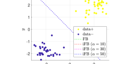
Figure 2: Data-set consisting of $80$ labeled points with given support vector-points $\pm(\frac{1}{2},\frac{3}{2})$ and $\pm(\frac{3}{2},\frac{1}{2})$. In dashed lines the (overlapping) max-margin separating hyperplanes formed by the last iterate of every scheme (Algorithms 1 and 2 with $\alpha=10$, $30$ and $50$ respectively).

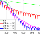
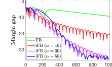
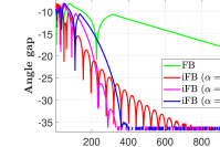
Figure 3: Values of the normalized error gap $\lvert{{w_{t}}/{\left\lVert{w_{t}}\right\rVert}-{w_{\ast}}/{\left\lVert{w_{\ast}}\right\rVert}}\rvert$ (first figure), the normalized margin gap ${M(w_{\ast})}{/\left\lVert{w_{\ast}}\right\rVert}-{M(w_{t})}/{\left\lVert{w_{t}}\right\rVert}$ (second figure) and the normalized angle gap $1-\frac{\left\langle{w_{t}},{w_{\ast}}\right\rangle}{\left\lVert{w_{t}}\right\rVert\left\lVert{w_{\ast}}\right\rVert}$ (third figure), as a function of the iterations $t$. Here we illustrate the performance of Algorithms 1(green) and 2 with $3$ different choices for the parameter $\alpha$ in Algorithm 2, $\alpha=10$ (red), $\alpha=30$ (magenta) and $\alpha=50$ (blue). As it appears in this example the choice of $\alpha$ decisively affects the performance of algorithm 2.

Second, we consider a data set of $1200$ points in $\mathbb{R}^{2}$, that consists of two classes distributed independently $\sim\mathcal{N}(\pm(\frac{1}{2},\frac{1}{2}),0.4)$ and we split them equally in training and test data. In this case, the training points are not linearly separable and algorithms 1 and 2 are implemented with a Gaussian kernel with parameter $\sigma^{2}=0.15$, see Remark 4.1. The total number of iterations (kernel evaluations) is set $T=2000$. In this experiment, we aim at illustrating convergence but also the stability of the proposed methods in the presence of the noise induced by mislabeling an amount of the training data. In particular, we are interested in the effect of the parameter $\lambda_{t}$ on the convergence behavior, as also on the stability performance of the proposed methods 1 and 2. In these experiments, the convergence is measured in terms of the margin, while the stability via the test error on the test data. In Figure 4, we plot the margin gap and the test error of Algorithms 1 and 2 with parameter $\lambda_{t}={\lambda_{0}}/{t}$ with $\lambda_{0}\in\{0.01,10,100\}$, for three different levels of noise ($p=$ percentage of flipped training labels) starting from $p=0\%$ (no noise), $p=10\%$ (moderate noise) and $p=20\%$ (strong noise). In Figure 5, we repeat the same experiment by choosing various orders of decay for $\lambda_{t}$, that is $\lambda_{t}\in\{{8}/{\log(t)},{8}/{\sqrt{t}},{8}/{t},{8}/{t^{2}},{8}/{2^{t}}\}$. Several comments can be made. First, we note that larger initialization $\lambda_{0}$ (e.g. $\lambda_{0}=100$ in Figure 4) or slower decay rate (e.g. $\lambda_{t}={8}/{\log(t)}$ or ${8}/{\sqrt{t}}$ in Figure 5) lead to slower margin convergence, but better generalization properties especially in presence of errors (second and third rows in Figures 4 and 5). In addition, while Algorithm 1 seems more robust with respect to the various changes of $\lambda_{t}$, the situation is different for the inertial variant 2. Both in Figures 4 and 5, for Algorithm 1, the behavior of the margin gap and the test error do not change radically unless the initialization is very large (e.g. $\lambda_{t}={100}/{t}$ in Figure 4) or the decay rate is very slow (e.g. $\lambda_{t}={8}/{\log(t)}$ or ${8}/{\sqrt{t}}$ in Figure 5) . On the other hand, Algorithm 2 seems more sensible to the different choices of the regularization parameter $\lambda_{t}$ both in terms of margin gap and test error.

In the noiseless case (first row in Figures 4 and 5) it seems that choosing $\lambda_{t}$ small enough (or decaying moderately fast to zero) can be a good policy. Note however that choosing too small initialization (or too fast decay to zero) does not offer any significant advantage with respect to more moderate choices of $\lambda_{t}$ (see in particular the blue, magenta and khaki lines in the first row of Figures 4 and 5 ). On the other hand, in presence of errors (second and third rows in Figures 4 and 5), larger initialization (like $\lambda_{0}=10$ or $1$ in Figure 4) and slower decay rate (as $\lambda_{t}={8}/{t}$ or ${8}/{\sqrt{t}}$ in Figure 5) may offer a better trade-off between margin convergence and test error.

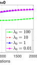
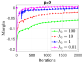
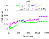
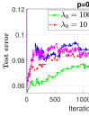
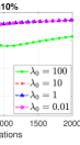
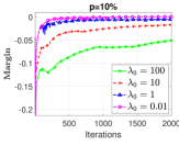
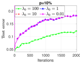
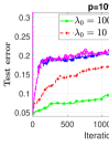
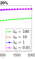
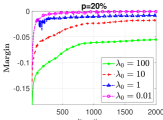
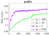
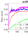
Figure 4: Margin and test error performance of Algorithms 1 and 2 in noisy dataset with $\lambda_{t}={\lambda_{0}}/{t}$, for different initial values of $\lambda_{0}$ ($\lambda_{0}=100$ in green, $\lambda_{0}=10$ in red, $\lambda_{0}=1$ in blue and $\lambda_{0}=0.01$ in magenta). Each row corresponds to a different noise level ($\%$ of flipped labels) starting with $0\%$ (first row), $10\%$ (second row) and $20\%$ (third row). The first and third column illustrate the margin and test error of Algorithm 1 respectively, while the second and the fourth column correspond to the margin (resp. test error) of Algorithm 2.

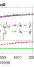
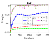
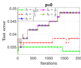
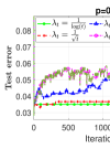
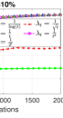
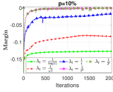
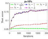
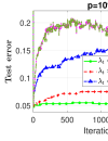
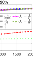
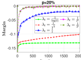
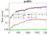
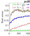
Figure 5: Margin and test error performance of Algorithms 1 and 2 in noisy dataset for different decay rates of $\lambda_{t}$ ($\lambda_{t}=\frac{\lambda_{0}}{\log(t)}$ in green, $\lambda_{t}=\frac{\lambda_{0}}{\sqrt{t}}$ in red, $\lambda_{t}=\frac{\lambda_{0}}{t}$ in blue, $\lambda_{t}=\frac{\lambda_{0}}{t^{2}}$ in magenta and $\lambda_{t}=\frac{\lambda_{0}}{2^{t}}$ in khaki), where $\lambda_{0}=8$. Each row corresponds to a different noise level ($\%$ of flipped labels) starting with $0\%$ (first row), $10\%$ (second row) and $20\%$ (third row). The first and third column illustrate the margin and test error of Algorithm 1 respectively, while the second and the fourth column correspond to the margin (resp. test error) of Algorithm 2.

6.2 Real data-set

Finally, we test the proposed methods on the MNIST dataset (see [46]) and on the HTRU$2$ dataset (see [49, 68]). In particular we compare the performance of Algorithms 1 and 2, with some of the recent proposed methods for binary classification [58, 79], and [40, 41] in terms of margin convergence and test error. The method in [58, 79] is a normalized gradient descent with variable stepsize on the exponential loss and the one in [40, 41] is based on an accelerated mirror descent approach on the smoothed margin of the exponential loss. We want to stress out that this comparison is indicative for the theoretical convergence properties of the tested methods and is not meant to be exhaustive. The results are reported in Figure 6.

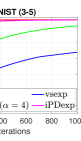
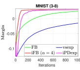
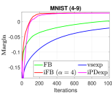
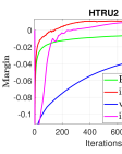
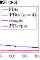
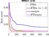
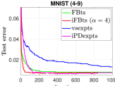
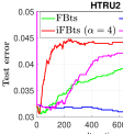
Figure 6: Margin and test error comparison on three pairs of MNIST digits (from first to third column) and the HTRU$2$ dataset (fourth column). The first row corresponds to margin gap, while the second one to the test error. In green and red are Algorithms 1 and 2 respectively. In blue is the variable stepsize normalized gradient method proposed in [79, 58] and in magenta the inertial mirror descent approach in [41].

All the data were standardized with zero mean and unit standard deviation and the binary labels of each dataset are set to be $-1$ and $1$. The MNIST dataset is restricted to a two-digits comparison of $3$ vs $5$, $3$ vs $8$ and $4$ vs $9$. For the HTRU$2$ dataset the training part was chosen by randomly picking $70\%$ of the whole dataset, while the test part is composed of the remaining $30\%$ (see e.g. [68]). All methods are implemented with the Gaussian kernel with parameter $\sigma^{2}=3.4$ for MNIST digits and $\sigma^{2}=4$ for the HTRU$2$ dataset. Each update use only the kernel evaluation and thus all the schemes have the same computational complexity per iteration. The test error is measured by the standard zero-one loss.

As a general remark Algorithm 2 has the best performance in terms of margin convergence and test error in the MNIST datasets. For HTRU$2$, while Algorithm 2 still provides the fastest margin convergence, it performs slightly worse than the method in [41] in terms of test error, whereas Algorithm 1 and the method proposed in [58] seem to give better test error results.

7 Conclusion and possible future work

In this work, we studied an iterative regularization procedure for classification with the hinge loss based on a dual diagonal process. We established new convergence results for a family of (inertial) diagonal proximal-gradient algorithms applied in the dual formulation of the penalized hinge loss, for solving the min-norm problem (MN) (equivalently the max-margin problem (MM)) for linear SVM problems. Inspired by the associated literature on dual diagonal methods in the inverse problem theory [31, 17], we were able to deduce new improved convergence rates for approaching the hard-margin solution (see Theorems 5.1 and 5.2). An interesting question for future work is to extend the study of iterative regularization in classification by incorporating different bias terms (possibly non-strongly convex) that lead to different notions of ”regular” separating solutions, rather than the one with minimal euclidean norm. In this setting different methods may be investigated like Mirror descent approaches or Primal-Dual schemes[54]. A question left for future study concerns the stability analysis of schemes like 1 and 2, in presence of possible errors coming from noisy data. In this setting, it would be interesting to deduce early-stopping criteria and study the possible trade-offs between precision and stability along the iterations. Finally, instead of considering linearly parametrized models, it would be interesting to further explore if similar ways of implicit regularization apply also for models with more complex structure, such as non-linearity or non-convexity, like neural networks. In particular, a starting point would be to consider general homogeneous models, like ReLU networks, as the ones considered in [69, 57].

Acknowledgements : We acknowledge the financial support of the European Research Council (grant SLING 819789), the AFOSR ((European Office of Aerospace Research and Development)) project FA9550-18-1-7009 and FA8655-22-1-7034, the EU H2020-MSCA-RISE project NoMADS - DLV-777826, the H2020-MSCA-ITN Project Trade-OPT 2019; L. R. acknowledges the Center for Brains, Minds and Machines (CBMM), funded by NSF STC award CCF-1231216 and IIT. S.V. is part of the Indam group “Gruppo Nazionale per l’Analisi Matematica, la Probabilità e le loro applicazioni”.

Appendix A Appendix

A.1 General Lemmas

In the following two lemmas we establish the regularization properties of Tikhonov regularization and gradient descent to the minimal norm interpolating solution, for general losses.

Lemma A.1 (Tikhonov).

Let $V:\mathbb{R}^{d}\to\mathbb{R}_{+}$ be a continuous and convex function. For all $\lambda>0$, consider:

$$w_{\lambda}=\operatornamewithlimits{arg\,min}_{w\in R^{d}}V(w)+\lambda\left\lVert{w}\right\rVert^{2}.$$ (A.1)

1. If $\operatornamewithlimits{arg\,min}V\neq\emptyset$, then

   $$\lim_{\lambda\to 0}w_{\lambda}=w^{\dagger}:=\operatornamewithlimits{arg\,min}\{\left\lVert{w}\right\rVert~{}:~{}w\in\operatornamewithlimits{arg\,min}V\}.$$

2. If $\operatornamewithlimits{arg\,min}V=\emptyset$, then $\left\lVert{w_{\lambda}}\right\rVert\underset{\lambda\to 0}{\to}+\infty$

Proof.

For the first point, let $w^{\ast}\in\operatornamewithlimits{arg\,min}V$ and $J_{\lambda}(w)=V(w)+\lambda\left\lVert{w}\right\rVert^{2}$. By the definition of $w_{\lambda}$ and $w^{\ast}$.

$$J_{\lambda}(w_{\lambda})\leq J_{\lambda}(w^{\ast})\leq V(w_{\lambda})+\lambda\left\lVert{w^{\ast}}\right\rVert^{2}$$

yielding

$$\left\lVert{w_{\lambda}}\right\rVert\leq\left\lVert{w^{\ast}}\right\rVert$$ (A.2)

which allows to deduce that the sequence $\{w_{\lambda}\}_{\lambda}{>0}$ is uniformly bounded. This implies that (up to a subsequence) $w_{\lambda}$ converges to an element $\bar{w}$. By lower semi-continuity of $V$, we have :

$$V(\bar{w})\leq\liminf V(w_{\lambda})\leq\liminf J_{\lambda}(w_{\lambda})\leq\liminf J_{\lambda}(w^{\dagger})=V(w^{\ast})$$

which shows that $\bar{w}\in\operatornamewithlimits{arg\,min}V$. In addition from the (weak) lower semi-continuity of the norm and relation (A.2), we have :

$$\left\lVert{\bar{w}}\right\rVert\leq\liminf\left\lVert{w_{\lambda}}\right\rVert\leq\left\lVert{w^{\ast}}\right\rVert$$

and since the last inequality holds for an arbitrary $w^{\ast}\in\operatornamewithlimits{arg\,min}V$, we deduce that $\bar{w}=w^{\dagger}$.

The second point can be proven by contrapositive. Let us assume the existence of some $M>0$, such that $\left\lVert{w_{\lambda}}\right\rVert\leq M$. By following the arguments of the proof of the first point, we deduce the existence of a limit point $w_{\lambda}\to\bar{w}\in\operatornamewithlimits{arg\,min}V$, which allows to conclude.

∎

Lemma A.2 (Gradient descent).

Let $X\in\mathbb{R}^{n\times d}$ be a linear operator, with $d>n$ , $y\in\Im(X)$ and $\mathcal{L}:\mathbb{R}^{n}\times\mathbb{R}^{n}\to\mathbb{R}_{+}$ be a proper, convex function with $L$-Lipschitz gradient, such that

$$(\forall(u,v)\in\mathbb{R}^{n}\times\mathbb{R}^{n})\quad\mathcal{L}(u,v)=0\Leftrightarrow u=v$$ (A.3)

Let also $w_{0}\in\Im(X^{\top})$, $0<\gamma\leq L\left\lVert{X}\right\rVert_{op}^{2}$ and consider the gradient iteration on the first argument of $\mathcal{L}\circ X$, i.e.

$$w_{t+1}=w_{t}-\gamma X^{\top}\nabla\mathcal{L}(Xw_{t},y)$$ (A.4)

Then

$$\lim_{t\to+\infty}w_{t}=w^{\dagger}:=\operatornamewithlimits{arg\,min}\{\left\lVert{w}\right\rVert~{}:~{}Xw=y\}$$ (A.5)

Proof.

First of all, since $d>n$, the set of minimizers of $\mathcal{L}(X\cdot,y)$ is non-empty (i.e. $\exists w\in\mathbb{R}^{d}$, such that $Xw=y$). By the standard gradient descent analysis (see for example [59, Paragraph $2.1.5$]), it holds that $w_{t}\underset{t\to\infty}{\to}\bar{w}\in\operatornamewithlimits{arg\,min}\mathcal{L}(X\cdot,y)$.

In addition, since $w_{0}\in\Im(X^{\top})$, by using (A.4), and a recurrence argument, we have that t$\{w_{t}\}_{t\geq 0}\in\Im(X^{\top})$. By closeness of $\Im(X^{\top})$, it follows that $\bar{w}\in\Im(X^{\top})$. By definition of $\mathcal{L}$, we have that the set of minimizers $\operatornamewithlimits{arg\,min}\mathcal{L}(X\cdot,y)=\{w~{}:~{}Xw=y\}$ is an affine space, hence it can be expressed as $\operatornamewithlimits{arg\,min}\mathcal{L}(X\cdot,y)={\operatorname{proj}_{\operatornamewithlimits{arg\,min}\mathcal{L}(X\cdot,y)}(0)}+V$, for some suitable space $V$, where $\operatorname{proj}_{\operatornamewithlimits{arg\,min}\mathcal{L}(X\cdot,y)}(0)$ denotes the projection of the $0$ element in $\operatornamewithlimits{arg\,min}\mathcal{L}(X\cdot,y)$ and is equal to $\{w^{\dagger}\}$, by definition.

Let us show that $V=\ker(X)$. Indeed for any $w\in\operatornamewithlimits{arg\,min}\mathcal{L}(X\cdot,y)$, we have $w=w^{\dagger}+v$, $v\in V$ and $y=Xw=Xw^{\dagger}+Xv=y+Xv$, which gives $V\subset\ker(X)$. On the other hand, if $u\in\ker(X)$ and $w^{\prime}=w^{\dagger}+u$, we have that $Xw^{\prime}=Xw^{\dagger}=y$, which allows to conclude that $\operatornamewithlimits{arg\,min}\mathcal{L}(X\cdot,y)=\{w^{\dagger}\}+\ker(X)$. By definition of the minimal norm solution it holds that $w^{\dagger}\in(\ker X)^{\perp}$ (see [27, Proposition $2.3$ and Theorem $2.5$]). By combining the facts $\bar{w}=w^{\dagger}+u$, $u\in\ker X$, $\bar{w}\in\Im(X^{\top})=(\ker X)^{\perp}$ and $w^{\dagger}\in(\ker X)^{\perp}$, it follows that $\bar{w}=w^{\dagger}$. ∎

The next lemma establishes the equivalence between the max-margin problem (MM) and the min-norm problem (MN). In fact the result holds true for general positively $1$-homogeneous features, i.e. by replacing $M(w)=\min_{i=1,\dots,n}y_{i}\left\langle{w},{x_{i}}\right\rangle$ in (MM) and (MN), by the general margin:

$$M(w)=\min_{i=1,\dots,n}y_{i}h_{i}(w).$$ (A.6)

Lemma A.3 (Max margin & min norm).

Let $h_{i}:\mathbb{R}^{d}\to\mathbb{R}$ be a family of positively $1$-homogeneous functions for all $i\leq n$ and consider the following optimization problems:

$$w_{+}=\operatornamewithlimits{arg\,max}\{M(w)=\min_{i=1,\dots,n}y_{i}h_{i}(w)~{}:~{}\left\lVert{w}\right\rVert=1\}$$ (A.7)

$$w_{\ast}=\operatornamewithlimits{arg\,min}\{\left\lVert{w}\right\rVert~{}:~{}M(w)=\min_{i=1,\dots,n}y_{i}h_{i}(w)\geq 1\}.$$ (A.8)

Then Problem (A.7) is equivalent to Problem (A.8). In particular, if $w_{\ast}$ is the solution of Problem (A.8) then $w_{+}=w_{\ast}/\left\lVert{w_{\ast}}\right\rVert$ is a solution of Problem (A.7). Further, if $w_{+}$ is the solution of Problem (A.7) then $w_{\ast}=\frac{w_{+}}{M(w_{+})}$ is a solution of Problem (A.8).

Proof.

First of all, from the definition of $M$, see (A.6), we have that for all $w\in\mathbb{R}^{d}\setminus\{0\}$

$$M(w)=\max_{\gamma>0}\gamma\qquad\text{s.t. }~{}\left\lVert{w}\right\rVert=1~{}~{}\&\quad y_{i}h_{i}(w)\geq\gamma,\qquad i=1,\dots,n.$$ (A.9)

By making the change of variable $w=\frac{w^{\prime}}{\left\lVert{w^{\prime}}\right\rVert}$ and taking into consideration (A.9), we can rewrite the max margin problem related to (A.7) as

$$\max_{w^{\prime}\in\mathbb{R}^{d}\setminus\{0\},\gamma>0}\gamma\qquad\text{s.t.}\qquad y_{i}h_{i}(w^{\prime}/\left\lVert{w^{\prime}}\right\rVert)\geq\gamma,\qquad i=1,\dots,n,$$

and using the homogeneity property of $h_{i}$,

$$\max_{w^{\prime}\in\mathbb{R}^{d}\setminus\{0\},\gamma>0}\gamma\qquad\text{s.t.}\qquad y_{i}\frac{1}{\left\lVert{w^{\prime}}\right\rVert}h_{i}(w^{\prime})\geq\gamma,\qquad i=1,\dots,n.$$ (A.10)

Then setting $\tilde{\gamma}=\gamma\left\lVert{w^{\prime}}\right\rVert$, (A.10) can be equivalently written as

$$\max_{w^{\prime}\in\mathbb{R}^{d}\setminus\{0\},\tilde{\gamma}>0}\frac{\tilde{\gamma}}{\left\lVert{w^{\prime}}\right\rVert}\qquad\text{s.t.}\qquad y_{i}h_{i}(w^{\prime})\geq\tilde{\gamma},\qquad i=1,\dots,n.$$ (A.11)

Since the above problem is still scale invariant by letting $v=\frac{w^{\prime}}{\tilde{\gamma}}$, (A.11) is equivalent to

$$\max_{v\in\mathbb{R}^{d}\setminus\{0\}}\frac{1}{\left\lVert{v}\right\rVert}\qquad\text{s.t.}\qquad y_{i}h_{i}(v)\geq 1,\qquad i=1,\dots,n.$$

which is equivalent to the min-norm problem related to  (A.8) (in the sense that the they have the same set of solutions) . By taking into consideration all the change of variables, it follows that $w_{+}=\frac{w_{\ast}}{\left\lVert{w_{\ast}}\right\rVert}$ and $w_{\ast}=\frac{w_{+}}{M(w_{+})}$, as also that $M(w_{\ast})=1$ and $M(w_{+})=\frac{1}{\left\lVert{w_{\ast}}\right\rVert}$. ∎

The following Lemma gives an expression of the dependence of the margin and the angle gap as a function of the gap of a method’s iterates approaching to the hard-margin solution $w_{\ast}$.

Lemma A.4 (Lemma $2$ [55]: Bounds for angle and margin).

Let $\delta>0$ and $c>0$, and $w_{\ast}\neq 0$ be the min-norm solution as defined in (MN). Let $\{w_{t}\}_{t\geq 1}$ be a sequence such that $\left\lVert{w_{t}}\right\rVert\geq\delta$. Then the following estimates hold true :

$$1-\frac{\left\langle{w_{t}},{w_{\ast}}\right\rangle}{\left\lVert{w_{t}}\right\rVert\left\lVert{w_{\ast}}\right\rVert}\leq\frac{1}{2\delta\left\lVert{w_{\ast}}\right\rVert}\left\lVert{w_{t}-w_{\ast}}\right\rVert^{2}$$ (A.12)

$$M\left(\frac{w_{\ast}}{\left\lVert{w_{\ast}}\right\rVert}\right)-M\left(\frac{w_{t}}{\left\lVert{w_{t}}\right\rVert}\right)\leq\frac{\left\lVert{X}\right\rVert_{F}}{\delta\left\lVert{w_{\ast}}\right\rVert}\left\lVert{w_{t}-w_{\ast}}\right\rVert$$ (A.13)

Proof.

Since $\left\lVert{w_{t}}\right\rVert\geq\delta$, by using the identity

$$\left\lVert{u-v}\right\rVert^{2}=\left\lVert{u}\right\rVert^{2}+\left\lVert{v}\right\rVert^{2}-2\left\langle{u},{v}\right\rangle\quad\forall u,v\in\mathbb{R}^{d}$$ (A.14)

we find :

$$1-\frac{\left\langle{w_{t}},{w_{\ast}}\right\rangle}{\left\lVert{w_{t}}\right\rVert\left\lVert{w_{\ast}}\right\rVert} =\frac{2\left\lVert{w_{t}}\right\rVert\left\lVert{w_{\ast}}\right\rVert+\left\lVert{w_{t}-w_{\ast}}\right\rVert^{2}-\left\lVert{w_{t}}\right\rVert^{2}-\left\lVert{w_{\ast}}\right\rVert^{2}}{2\left\lVert{w_{t}}\right\rVert\left\lVert{w_{\ast}}\right\rVert}=\frac{\left\lVert{w_{t}-w_{\ast}}\right\rVert^{2}-\big{(}\left\lVert{w_{t}}\right\rVert-\left\lVert{w_{\ast}}\right\rVert\big{)}^{2}}{2\left\lVert{w_{t}}\right\rVert\left\lVert{w_{\ast}}\right\rVert}$$ (A.15)

$$\leq\frac{1}{2\delta\left\lVert{w_{\ast}}\right\rVert}\left\lVert{w_{t}-w_{\ast}}\right\rVert^{2}$$

which allow to prove the first point.

Finally if $j=\operatornamewithlimits{arg\,min}_{i\leq n}\{y_{i}\left\langle{w_{t}},{x_{i}}\right\rangle\}$, then by definition of the margin $M$ and $w_{\ast}$, since $M(w_{\ast})=1$ (see Lemma 3.1), we obtain:

$$M\left(\frac{w_{\ast}}{\left\lVert{w_{\ast}}\right\rVert}\right)-M\left(\frac{w_{t}}{\left\lVert{w_{t}}\right\rVert}\right) =\frac{1}{\left\lVert{w_{\ast}}\right\rVert}-\frac{y_{j}\left\langle{w_{t}},{x_{j}}\right\rangle}{\left\lVert{w_{t}}\right\rVert}\leq\frac{y_{j}\left\langle{w_{\ast}},{x_{j}}\right\rangle}{\left\lVert{w_{\ast}}\right\rVert}-\frac{y_{j}\left\langle{w_{t}},{x_{j}}\right\rangle}{\left\lVert{w_{t}}\right\rVert}=y_{j}\left\langle{\frac{w_{\ast}}{\left\lVert{w_{\ast}}\right\rVert}-\frac{w_{t}}{\left\lVert{w_{t}}\right\rVert}},{x_{j}}\right\rangle$$ (A.16)

$$\leq\left\lVert{\frac{w_{\ast}}{\left\lVert{w_{\ast}}\right\rVert}-\frac{w_{t}}{\left\lVert{w_{t}}\right\rVert}}\right\rVert\left\lVert{x_{j}}\right\rVert\leq\left\lVert{X}\right\rVert_{F}\left\lVert{\frac{w_{\ast}}{\left\lVert{w_{\ast}}\right\rVert}-\frac{w_{t}}{\left\lVert{w_{t}}\right\rVert}}\right\rVert$$

and since

$$\left\lVert{\frac{w_{t}}{\left\lVert{w_{t}}\right\rVert}-\frac{w_{\ast}}{\left\lVert{w_{\ast}}\right\rVert}}\right\rVert^{2}=1+1-2\frac{\left\langle{w_{t}},{w_{\ast}}\right\rangle}{\left\lVert{w_{t}}\right\rVert\left\lVert{w_{\ast}}\right\rVert}=2\bigg{(}1-\frac{\left\langle{w_{t}},{w_{\ast}}\right\rangle}{\left\lVert{w_{t}}\right\rVert\left\lVert{w_{\ast}}\right\rVert}\bigg{)}$$ (A.17)

the conclusion follows by combining (A.15) and (A.16). ∎

The next lemma is a general descent lemma that is classically used for proximal gradient methods applied to structured composite convex optimization problems, such as (4.9). The interested reader can find a proof in [11, Lemma $2.3$]

Lemma A.5.

Let $F=f+g:\mathbb{R}^{n}\longrightarrow\mathbb{R}$, where $f$ and $g$ are convex lower-semi continuous function and $f$ is continuously differentiable with $L$-Lipschitz gradient. For all $0<\gamma\leq\frac{1}{L}$, consider the operator $T_{\gamma}:\mathbb{R}^{n}\longrightarrow\mathbb{R}^{n}$, such that $T_{\gamma}(x):=\operatorname{prox}_{\gamma g}\big{(}x-\gamma\nabla f(x)\big{)}$. Then for all $(x,y)\in(\mathbb{R}^{n})^{2}$ it holds:

$$2\gamma\big{(}F(T_{\gamma}(y))-F(x)\big{)}\leq\left\lVert{y-x}\right\rVert^{2}-\left\lVert{T_{\gamma}(y)-x}\right\rVert^{2}$$ (A.18)

A.2 Proofs of Section 5.2

Proof of Lemma 5.1.

Since $\lambda_{t}$ is non-increasing, for every $u\in\mathbb{R}^{n}$ it follows that the function $t\mapsto\frac{1}{\lambda_{t}}\mathcal{L}^{\ast}(\lambda_{t}u)=\sum_{i=1}^{n}u^{i}+\iota_{[-1,0]}(\lambda_{t}u^{i})$ is non-increasing in $[0,+\infty]$.

In addition, by direct computation for all $u\in\mathbb{R}^{n}$, it holds:

$$\frac{1}{\lambda_{t}}\mathcal{L}^{\ast}(\lambda_{t}u)=\sum_{i=1}^{n}u^{i}+\iota_{(-1,0]^{n}}(\lambda_{t}u)\underset{t\to\infty}{\longrightarrow}\sum_{i=1}^{n}u^{i}+\iota_{(-\infty,0]^{n}}(u)$$ (A.19)

Thus, for all $u\in\mathbb{R}^{n}$, the function $D_{t}(u)$ is non-increasing in $t\geq 0$ and that $D_{t}(u)\underset{t\to\infty}{\longrightarrow}D_{\infty}(u).$ ∎

Proof of Lemma 5.2.

From the separability assumption (1) there exists some $\tilde{w}\in\mathbb{R}^{d}$, such that $\left\langle{\tilde{w}},{x_{i}}\right\rangle>0~{},\forall i\leq n$. Let $i_{min}=\operatornamewithlimits{arg\,min}\{\left\langle{\tilde{w}},{x_{i}}\right\rangle~{}:~{}i\leq n\}$ and let $M(\tilde{w})=\left\langle{\tilde{w}},{x_{i_{min}}}\right\rangle>0$. Then by setting $w^{\prime}=\frac{2\tilde{w}}{M(\tilde{w})}$, we have $\left\langle{w^{\prime}},{x_{i}}\right\rangle=\frac{\left\langle{2\tilde{w}},{x_{i}}\right\rangle}{M(\tilde{w})}\geq 2>1~{},~{}\forall i\leq n$. Thus we deduce the existence of an element $w^{\prime}\in\text{dom}\frac{\left\lVert{\cdot}\right\rVert^{2}}{2}=\mathbb{R}^{n}$, such that $\mathcal{L}$ is continuous at $Xw^{\prime}$ (since $\mathcal{L}$ is continuous and $w^{\prime}\in\text{dom}\mathcal{L}$). By [65, Corollary $3.31$] and the optimality condition for the min-norm separating solution $w_{\ast}$, the sum rule for the subdifferential holds and thus we have

$$0\in\partial\left(\frac{\left\lVert{\cdot}\right\rVert^{2}}{2}\ +\iota_{[1,+\infty)^{n}}\circ X\right)(w_{\ast})=\nabla\left(\frac{\left\lVert{\cdot}\right\rVert^{2}}{2}\right)(w_{\ast})+X^{\top}\partial\iota_{[1,+\infty)^{n}}(Xw_{\ast})=\{w_{\ast}\}+X^{\top}X^{\top}\partial\iota_{[1,+\infty)^{n}}(Xw_{\ast})$$ (A.20)

From (A.20), there exists some $u_{\ast}\in\partial\iota_{[1,+\infty)^{n}}(Xw_{\ast})$ such that $w_{\ast}=-X^{\top}u_{\ast}$ or equivalently $Xw_{\ast}\in\partial\iota^{\ast}_{[1,+\infty)^{n}}(u_{\ast})$. Hence, by replacing $w_{\ast}=-X^{\top}u_{\ast}$, we obtain:

$$-XX^{\top}u_{\ast}\in\partial\iota^{\ast}_{[1,+\infty)^{n}}(u_{\ast})~{}\Leftrightarrow~{}$$ (A.21)

$$~{}\Leftrightarrow~{}0\in-X\nabla\left(\frac{\left\lVert{\cdot}\right\rVert^{2}}{2}\right)(-X^{\top}u_{\ast})+\partial\iota^{\ast}_{[1,+\infty)^{n}}(u_{\ast})\subset\partial\left(\frac{\left\lVert{-X^{\top}\cdot}\right\rVert^{2}}{2}+\iota^{\ast}_{[1,+\infty)^{n}}(\cdot)\right)(u_{\ast})$$

which shows that $u_{\ast}\in\operatornamewithlimits{arg\,min}D_{\infty}$. In order to prove (5.14), let $u\in\mathbb{R}^{n}$ and $w=-X^{\top}u$.

Since $Xw_{\ast}\in\partial\iota_{[1,+\infty)^{n}}(u_{\ast})$ and $-X^{\top}u=w$, by using the Fenchel-Young equality for $\frac{\left\lVert{-X^{\top}u_{\ast}}\right\rVert^{2}}{2}$and $\frac{\left\lVert{-X^{\top}u}\right\rVert^{2}}{2}$, we find:

$$D_{\infty}(u)-D_{\infty}(u_{\ast}) =\frac{\left\lVert{-X^{\top}u}\right\rVert^{2}}{2}-\frac{\left\lVert{-X^{\top}u_{\ast}}\right\rVert^{2}}{2}+\iota^{\ast}_{[1,+\infty)^{n}}(u)-\iota^{\ast}_{[1,+\infty)^{n}}(u_{\ast})$$ (A.22)

$$=\left\langle{-X^{\top}u},{w}\right\rangle-\frac{\left\lVert{w}\right\rVert^{2}}{2}+\left\langle{X^{\top}u_{\ast}},{w_{\ast}}\right\rangle+\frac{\left\lVert{w_{\ast}}\right\rVert^{2}}{2}+\iota^{\ast}_{[1,+\infty)^{n}}(u)-\iota^{\ast}_{[1,+\infty)^{n}}(u_{\ast})$$

$$=\frac{\left\lVert{w_{\ast}}\right\rVert^{2}}{2}-\frac{\left\lVert{w}\right\rVert^{2}}{2}-\left\langle{-X^{\top}u},{w_{\ast}-w}\right\rangle$$

$$\quad+\iota^{\ast}_{[1,+\infty)^{n}}(u)-\iota^{\ast}_{[1,+\infty)^{n}}(u_{\ast})-\left\langle{Xw_{\ast}},{u-u_{\ast}}\right\rangle$$

By using the strong convexity of $\frac{\left\lVert{\cdot}\right\rVert^{2}}{2}$ (with parameter $1$) and the convexity of $\iota^{\ast}_{[1,+\infty)^{n}}(\cdot)$, we conclude that:

$$D_{\infty}(u)-D_{\infty}(u_{\ast})\geq\frac{\left\lVert{w-w_{\ast}}\right\rVert^{2}}{2}$$ (A.23)

∎

Proof of Lemma 5.3.

Let $u_{\ast}\in\operatornamewithlimits{arg\,min}D_{\infty}$. Since $\frac{\left\lVert{\cdot}\right\rVert^{2}}{2}\circ X^{\top}$ has $\left\lVert{XX^{\top}}\right\rVert_{op}$-Lipschitz gradient, by applying the Descent Lemma A.5 with $y=u_{t}$, for all $u\in\mathbb{R}^{n}$ and $t\geq 0$ it holds:

$$D_{t}(u_{t+1})+\frac{1}{2\gamma}\left\lVert{u_{t+1}-u}\right\rVert^{2}\leq D_{t}(u)+\frac{1}{2\gamma}\left\lVert{u_{t}-u}\right\rVert^{2}$$ (A.24)

which allows to deduce (5.16).

By choosing $u=u_{t}$ in (A.24) and using the non-increasing property of $D_{t}$ in $t\geq 0$ (see Lemma 5.1), we obtain:

$$D_{t+1}(u_{t+1})-D_{\infty}(u_{\ast})\leq D_{t}(u_{t+1})-D_{\infty}(u_{\ast})\leq D_{t}(u_{t})-D_{\infty}(u_{\ast})-\frac{1}{2\gamma}\left\lVert{u_{t+1}-u_{t}}\right\rVert^{2}$$ (A.25)

which shows that the function $r_{t}=D_{t}(u_{t})-D_{\infty}(u_{\ast})$ is non-increasing in $t$. Since $D_{t}(u)$ is also non-increasing in $t$ and convergent to $D_{\infty}(u)$, from (A.24) we also have that $\frac{1}{2\gamma}\left\lVert{u_{t}-u}\right\rVert^{2}$ is bounded for all $u\in\mathbb{R}^{n}$. In addition $r_{t}=D_{t}(u_{t})-D_{\infty}(u_{\ast})\geq D_{\infty}(u_{t})-D_{\infty}(u_{\ast})\geq 0$, which shows that $r_{t}$ is also bounded from below by zero, and therefore converges to a non-negative limit.

By adding and subtracting $D_{\infty}(u_{\ast})$ in (A.24), for all $u\in\mathbb{R}^{n}$, we find:

$$r_{t+1}-(D_{t}(u)-D_{\infty}(u_{\ast}))\leq\frac{1}{2\gamma}\left\lVert{u_{t}-u}\right\rVert^{2}-\frac{1}{2\gamma}\left\lVert{u_{t+1}-u}\right\rVert^{2}$$ (A.26)

which by summing up to $t\geq 1$ gives:

$$\sum_{s=1}^{t}\big{(}r_{s}-(D_{s-1}(u)-D_{\infty}(u_{\ast}))\big{)}\leq\frac{1}{2\gamma}\left\lVert{u_{0}-u}\right\rVert^{2}\quad\forall u\in\mathbb{R}^{n}$$ (A.27)

The last relation allows to conclude that $\lim\limits_{t\to\infty}\big{(}r_{t}-(D_{t-1}(u)-D_{\infty}(u_{\ast}))\big{)}=0$ and since $\lim\limits_{t\to\infty}D_{t-1}(u)=D_{\infty}(u)\geq D_{\infty}(u_{\ast})$ and $\lim\limits_{t\to\infty}r_{t}\geq 0$, we have that $\lim\limits_{t\to\infty}r_{t}=0$. ∎

The proof of Lemma 5.4 is inspired by the analysis presented in [10, Lemma $2.5$] with some modifications. More precisely we will prove that there exists some positive constants $M,~{}R,~{}\theta$, such that for all $t\geq 0$, $D_{t}$ satisfies the following growth condition:

$$\left(\forall u\in[D_{t}\leq\min D_{t}+M]\cap\mathbb{B}(\mathbf{0},R)\right),\qquad\frac{\theta}{2}\text{dist}\left({u,\operatornamewithlimits{arg\,min}D_{t}}\right)^{2}\leq D_{t}(u)-\min D_{t}$$ (A.28)

It is worth mentioning that we cannot apply directly the proof in [10, Lemma $2.5$], due to the fact of possible unboudedness of $\operatornamewithlimits{arg\,min}D_{t}$, when $t\to\infty$. Indeed by applying directly [10, Lemma $2.5$] we can deduce the existence of $\theta_{t}$, such that (A.28) hold true. However this is not sufficient for establishing linear convergence of the proposed scheme (see Proposition 5.1).

Proof of Lemma 5.4.

For all $t\geq 0$, the problem $\underset{u\in\mathbb{R}^{n}}{\min}D_{t}(u)$ is equivalent to the following constrained optimization one:

$$\min\left\{F(u):=\frac{1}{2}\left\lVert{X^{\top}u}\right\rVert^{2}+\left\langle{\bf{1}},{u}\right\rangle~{}:~{}u\in\mathcal{U}_{t}:=[-\lambda_{t},0]^{n}\right\}.$$ (A.29)

If $u\notin\mathcal{U}_{t}$, relation (A.28) holds, so without loss of generality, we assume that $u\in\mathcal{U}_{t}$, so that $F(u)=D_{t}(u)$.

For all $t\geq 0$, let $\bar{u}_{t}\in\underset{u\in\mathbb{R}^{n}}{\operatornamewithlimits{arg\,min}}D_{t}(u)$. By the optimality conditions for problem (A.29), for all $u\in\mathcal{U}_{t}$, it holds:

$$\left\langle{\nabla F(\bar{u}_{t})},{u-\bar{u}_{t}}\right\rangle\geq 0$$ (A.30)

Notice that $\mathcal{U}_{t}$ is a polyhedral set since $\mathcal{U}_{t}=\{u\in\mathbb{R}^{n}~{}:~{}Au\leq a_{t}\}$, with $A=\begin{bmatrix}\text{Id}_{n}\\ -\text{Id}_{n}\end{bmatrix}\in\mathbb{R}^{2n\times n}$ and $a_{t}=-\lambda_{t}^{-1}\begin{bmatrix}\mathbf{0}\\ \mathbf{1}\end{bmatrix}\in\mathbb{R}^{2n}$.

By [10, Lemma $2.3$ ], there exist a unique vector $\bar{v}\in\mathbb{R}^{n}$ and a scalar $\bar{s}\in\mathbb{R}$ such that the following equivalence holds true:

$$\bar{u}_{t}\in\operatornamewithlimits{arg\,min}D_{t}~{}\Leftrightarrow~{}\begin{bmatrix}X^{\top}\\ \mathbf{1}^{\top}\end{bmatrix}\bar{u}_{t}=\begin{bmatrix}\bar{v}\\ \bar{s}\end{bmatrix}\quad\text{and }\quad A\bar{u}_{t}\leq a_{t}$$ (A.31)

so that $\operatornamewithlimits{arg\,min}D_{t}=S\cap\mathcal{U}_{t}$, where $S=\left\{u\in\mathbb{R}^{n}~{}:\begin{bmatrix}X^{\top}\\ \mathbf{1}^{\top}\end{bmatrix}u=\begin{bmatrix}\bar{v}\\ \bar{s}\end{bmatrix}\right\}$ and $\mathcal{U}_{t}=\{u\in\mathbb{R}^{n}~{}:Au\leq a_{t}\}$.

According to Hoffman’s lemma [39] (see also [85, Lemma $15$]) for the polyhedral sets $S$ and $\mathcal{U}_{t}$, by setting $E=\begin{bmatrix}X^{\top}\\ \mathbf{1}^{\top}\end{bmatrix}\in\mathbb{R}^{(d+1)\times n}$, there exists some positive constant $\tau$ given by (5.3), such that

$$\text{dist}\left(u,\operatornamewithlimits{arg\,min}D_{t}\right)=\text{dist}\left(u,S\cap\mathcal{U}_{t}\right)\leq\tau\left\lVert{Eu-\begin{bmatrix}\bar{v}\\ \bar{s}\end{bmatrix}}\right\rVert$$ (A.32)

It is important to stress out that the Hoffman’s error bound constant $\tau$ only depends on the matrices $E$ and $A$ (see e.g. [87, Remark $1$] and the associated references). In our setting this means that the constant $\tau$ only depends on the data-matrix $X$.

By taking the squares in (A.32), we find:

$$\text{dist}\left(u,\operatornamewithlimits{arg\,min}D_{t}\right)^{2}\leq\tau^{2}\left(\left\lVert{X^{\top}(u-\bar{u}_{t})}\right\rVert^{2}+(\left\langle{1},{u-\bar{u}_{t}}\right\rangle)^{2}\right)$$ (A.33)

Let us now bound appropriately the two terms in the right-hand-side of (A.33).

For the first term, by developing the square we find:

$$\frac{1}{2}\left\lVert{X^{\top}(u-\bar{u}_{t})}\right\rVert^{2} =\frac{1}{2}\left\lVert{X^{\top}u}\right\rVert^{2}-\left\langle{X^{\top}u},{X^{\top}\bar{u}_{t}}\right\rangle+\frac{1}{2}\left\lVert{X^{\top}\bar{u}_{t}}\right\rVert^{2}$$ (A.34)

$$=\frac{1}{2}\left\lVert{X^{\top}u}\right\rVert^{2}-\frac{1}{2}\left\lVert{X^{\top}\bar{u}_{t}}\right\rVert^{2}-\left\langle{X^{\top}\bar{u}_{t}},{X^{\top}(u-\bar{u}_{t})}\right\rangle$$

$$\leq\left\langle{\nabla F(\bar{u}_{t})},{u-\bar{u}_{t}}\right\rangle+\frac{1}{2}\left\lVert{X^{\top}u}\right\rVert^{2}-\frac{1}{2}\left\lVert{X^{\top}\bar{u}_{t}}\right\rVert^{2}-\left\langle{X^{\top}\bar{u}_{t}},{X^{\top}(u-\bar{u}_{t})}\right\rangle$$

where in the last inequality we used the optimality condition (A.30). In addition, since $\nabla F(\bar{u}_{t})=\mathbf{1}+XX^{\top}\bar{u}_{t}$, from (A.34) it follows:

$$\frac{1}{2}\left\lVert{X^{\top}(u-\bar{u}_{t})}\right\rVert^{2}\leq\frac{1}{2}\left\lVert{X^{\top}u}\right\rVert^{2}+\left\langle{\mathbf{1}},{u}\right\rangle-\frac{1}{2}\left\lVert{X^{\top}\bar{u}_{t}}\right\rVert^{2}-\left\langle{\mathbf{1}},{\bar{u}_{t}}\right\rangle=D_{t}(u)-\min D_{t}$$ (A.35)

Let us now provide an upper bound for the term $(\left\langle{1},{u-\bar{u}_{t}}\right\rangle)^{2}$. On the one hand we have:

$$\left\langle{\bf{1}},{\bar{u}_{t}-u}\right\rangle =\left\langle{\nabla F(\bar{u}_{t})},{\bar{u}_{t}-u}\right\rangle-\left\langle{X^{\top}\bar{u}_{t}},{X^{\top}(\bar{u}_{t}-u)}\right\rangle$$ (A.36)

$$=\left\langle{\nabla F(\bar{u}_{t})},{\bar{u}_{t}-u}\right\rangle-\left\lVert{X^{\top}(u-\bar{u}_{t})}\right\rVert^{2}+\left\langle{X^{\top}u},{X^{\top}(\bar{u}_{t}-u)}\right\rangle$$

$$\leq\left\langle{\nabla F(\bar{u}_{t})},{\bar{u}_{t}-u}\right\rangle+\left\lVert{X^{\top}u}\right\rVert\left\lVert{X^{\top}(\bar{u}_{t}-u)}\right\rVert$$

$$\leq\left\lVert{X^{\top}u}\right\rVert\left\lVert{X^{\top}(\bar{u}_{t}-u)}\right\rVert$$

where in the first inequality we used the Cauchy-Schwarz inequality and for the last one the optimality condition (A.30). On the other hand we find:

$$\left\langle{\bf{1}},{u-\bar{u}_{t}}\right\rangle =\left\langle{\nabla F(\bar{u}_{t})},{u-\bar{u}_{t}}\right\rangle-\left\langle{X^{\top}\bar{u}_{t}},{X^{\top}(u-\bar{u}_{t})}\right\rangle$$ (A.37)

$$=\left\langle{\nabla F(\bar{u}_{t})},{u-\bar{u}_{t}}\right\rangle+\left\lVert{X^{\top}(u-\bar{u}_{t})}\right\rVert^{2}-\left\langle{X^{\top}u},{X^{\top}(u-\bar{u}_{t})}\right\rangle$$

$$\leq\left\langle{\nabla F(\bar{u}_{t})},{u-\bar{u}_{t}}\right\rangle+\left\lVert{X^{\top}(u-\bar{u}_{t})}\right\rVert^{2}+\left\lVert{X^{\top}u}\right\rVert\left\lVert{X^{\top}(u-\bar{u}_{t})}\right\rVert$$

$$=\left\langle{\nabla F(\bar{u}_{t})},{u-\bar{u}_{t}}\right\rangle+\left(\left\lVert{X^{\top}(u-\bar{u}_{t})}\right\rVert+\left\lVert{X^{\top}u}\right\rVert\right)\left\lVert{X^{\top}(u-\bar{u}_{t})}\right\rVert$$

$$\leq D_{t}(u)-\min D_{t}+\left(\left\lVert{X^{\top}(u-\bar{u}_{t})}\right\rVert+\left\lVert{X^{\top}u}\right\rVert\right)\left\lVert{X^{\top}(u-\bar{u}_{t})}\right\rVert$$

where in the first inequality we used the Cauchy-Schwarz inequality and in the last one the convexity of $F$. By relations (A.36) and (A.37), it follows that:

$$\lvert{\left\langle{\bf{1}},{u-\bar{u}_{t}}\right\rangle}\rvert \leq D_{t}(u)-\min D_{t}+\left(\left\lVert{X^{\top}(u-\bar{u}_{t})}\right\rVert+\left\lVert{X^{\top}u}\right\rVert\right)\left\lVert{X^{\top}(u-\bar{u}_{t})}\right\rVert$$ (A.38)

$$\leq\left(3\sqrt{D_{t}(u)-\min D_{t}}+\sqrt{2}\left\lVert{X^{\top}u}\right\rVert\right)\sqrt{D_{t}(u)-\min D_{t}}$$

$$\leq\left(3\sqrt{M}+\sqrt{2}R\left\lVert{X}\right\rVert_{\text{op}}\right)\sqrt{D_{t}(u)-\min D_{t}}$$

where in the second inequality we used (A.35) and in the last one the fact that $u\in[D_{t}\leq\min D_{t}+M]\cap\mathbb{B}(0,R)$. By injecting relations (A.35) and (A.38) into (A.33), for all $u\in[D_{t}\leq\min D_{t}+M]\cap\mathbb{B}(0,R)$ we find:

$$\text{dist}\left(u,\operatornamewithlimits{arg\,min}D_{t}\right)^{2} \leq\tau^{2}\left(2\left(D_{t}(u)-\min D_{t}\right)+\left(3\sqrt{M}+\sqrt{2}R\left\lVert{X}\right\rVert_{\text{op}}\right)^{2}\left(D_{t}(u)-\min D_{t}\right)\right)$$ (A.39)

$$=\tau^{2}\left(9M+6\sqrt{2M}R\left\lVert{X}\right\rVert_{\text{op}}+2R^{2}\left\lVert{X}\right\rVert_{\text{op}}^{2}+2\right)\left(D_{t}(u)-\min D_{t}\right)$$

which shows that for all $t\geq 0$, $D_{t}$ satisfies the growth condition (A.28) in $[D_{t}\leq\min D_{t}+M]\cap\mathbb{B}(0,R)$, with $\theta=\left(2\tau^{2}\left(9M+6\sqrt{2M}R\left\lVert{X}\right\rVert_{\text{op}}+2R^{2}\left\lVert{X}\right\rVert_{\text{op}}^{2}+2\right)\right)^{-1}$

Finally by using the equivalence between the $\theta$-growth condition (A.28) and the $\mu$-Łojasiewicz condition (5.1) with $\mu=\frac{\theta}{4}$ (see e.g. [3, Proposition $1$] or [12, Theorem $5$]), we deduce that for all $t\geq 0$, $D_{t}$ satisfies (5.1), with

$$\mu=\frac{1}{8\tau^{2}\left(9M+6\sqrt{2M}R\left\lVert{X}\right\rVert_{\text{op}}+2R^{2}\left\lVert{X}\right\rVert_{\text{op}}^{2}+2\right)}$$ (A.40)

and $\tau$ is the Hoffman’s constant as defined in (5.3). ∎

Proof of Proposition 5.1.

Let $u_{\ast}\in\operatornamewithlimits{arg\,min}D_{\infty}$ and $\lambda_{0}>0$, such that $\lambda_{0}\leq\left\lVert{u_{\ast}}\right\rVert^{-1}$. Following the proof of Lemma 5.3, by choosing $u=u_{\ast}$ in (A.24), we find:

$$D_{t}(u_{t+1})-D_{t}(u_{\ast})+\frac{1}{2\gamma}\left\lVert{u_{t+1}-u_{\ast}}\right\rVert^{2}\leq\frac{1}{2\gamma}\left\lVert{u_{t}-u_{\ast}}\right\rVert^{2}$$ (A.41)

Since $D_{t}(u_{\ast})\leq D_{t}(u)$, for all $u\in\mathbb{R}^{n}$, by neglecting the non-negative term and summing over $t\geq 0$ relation (A.41), we deduce that for all $t\geq 0$ it holds $\left\lVert{u_{t}-u_{\ast}}\right\rVert\leq\left\lVert{u_{0}-u_{\ast}}\right\rVert$, therefore the sequence $\{u_{t}\}_{t\geq 0}$ is bounded by $R=2\left\lVert{u_{\ast}}\right\rVert+\left\lVert{u_{0}}\right\rVert$.

On the other hand, by choosing $u=u_{t}$ in (A.24)and using the non-increasing property of $D_{t}$ (Lemma 5.1), we find:

$$D_{t+1}(u_{t+1})-D_{t}(u_{t})\leq D_{t}(u_{t+1})-D_{t}(u_{t})\leq-\frac{1}{2\gamma}\left\lVert{u_{t+1}-u_{t}}\right\rVert^{2}$$ (A.42)

which allows to conclude that the sequence $\{u_{t}\}_{t\geq 0}\in[D_{t}\leq D_{0}(u_{0})]=\{u\in\mathbb{R}^{n}~{}:~{}D_{t}(u)\leq D_{0}(u_{0})\}$.

By definition of $u_{t+1}=\lambda_{t}^{-1}\operatorname{prox}_{\gamma\lambda_{t}\mathcal{L}^{\ast}}\left(\lambda_{t}\left(u_{t}-\gamma XX^{\top}u_{t}\right)\right)$ (see Algorithm 1) and the characterization of the proximal operator, for all $t\geq 0$, we have $\lambda_{t}u_{t+1}+\gamma\lambda_{t}\partial\mathcal{L}^{\ast}(\lambda_{t}u_{t+1})\ni\lambda_{t}\left(u_{t}-\gamma XX^{\top}u_{t}\right)$ or equivalently

$$\left(\text{Id}-\gamma XX^{\top}\right)(u_{t}-u_{t+1})\in\gamma\partial\mathcal{L}^{\ast}(\lambda_{t}u_{t+1})+\gamma XX^{\top}u_{t+1}=\partial\gamma D_{t}(u_{t+1})$$ (A.43)

Hence (A.43) together with the contraction property of the operator $\text{Id}-\gamma XX^{\top}$ for all $\gamma\leq\frac{1}{\left\lVert{XX^{\top}}\right\rVert}$, yields:

$$\text{dist}\left(\partial D_{t}(u_{t+1}),0\right)\leq\gamma^{-1}\left\lVert{\left(\text{Id}-\gamma XX^{\top}\right)(u_{t}-u_{t+1})}\right\rVert\leq\gamma^{-1}\left\lVert{u_{t+1}-u_{t}}\right\rVert$$ (A.44)

By combining relations (A.42) and (A.44), we obtain:

$$D_{t}(u_{t+1})-D_{t}(u_{t})\leq-\frac{\gamma}{2}\text{dist}\left(\partial D_{t}(u_{t+1}),0\right)^{2}$$ (A.45)

Since $u_{t}\in[D_{t}\leq\min D_{t}+M]\cap\mathbb{B}_{R}(\mathbf{0})$ with $M=D_{0}(u_{0})-D_{\infty}(u_{\ast})$ and $R=\left\lVert{u_{0}}\right\rVert+2\left\lVert{u_{\ast}}\right\rVert$, by using (5.1) and Lemma 5.4 we find:

$$D_{t}(u_{t+1})-D_{t}(u_{t})\leq-\gamma\mu\left(D_{t}(u_{t+1})-\min D_{t}(u)\right)$$ (A.46)

By adding and subtracting $D_{\infty}(u_{\ast})$ and using that $D_{t+1}(u_{t+1})\leq D_{t}(u_{t+1})$ and $D_{\infty}(u)\leq\min D_{t}(u)$ (see Lemma 5.1), for all $t\geq 1$, we derive:

$$(1+\gamma\mu)\left(D_{t+1}(u_{t+1})-D_{\infty}(u_{\ast})\right)\leq\left(D_{t}(u_{t})-D_{\infty}(u_{\ast})\right)$$ (A.47)

By induction in (A.47), for all $t\geq 0$, it follows

$$D_{t}(u_{t})-D_{\infty}(u_{\ast})\leq\left(D_{0}(u_{0})-D_{\infty}(u_{\ast})\right)\left(1-\frac{\gamma\mu}{1+\gamma\mu}\right)^{t}$$ (A.48)

which allows to conclude the proof. ∎

Proof of Proposition 5.2.

Let $u_{\ast}\in\operatornamewithlimits{arg\,min}D_{\infty}$ and $u_{t}$ the sequence generated by Algorithm 2 with $\lambda_{0}\leq\left\lVert{u_{\ast}}\right\rVert^{-1}$. For all $\nu>0$, let us define the following auxiliary sequences:

$$r_{t} =D_{t}(u_{t})-D_{\infty}(u_{\ast})~{},\quad\delta_{t}=\left\lVert{u_{t}-u_{t-1}}\right\rVert^{2}~{},\quad h_{t}=\left\lVert{u_{t}-u_{\ast}}\right\rVert^{2}$$ (A.49)

$$k_{t} =t+\alpha-1~{}\text{ and }~{}v_{t}=\left\lVert{\nu(u_{t-1}-u_{+})+k_{t}(u_{t}-u_{t-1})}\right\rVert^{2}$$ (A.50)

The following energy sequence that will play a fundamental role in our analysis

$$E_{t} =(t+\alpha-1)^{2}\big{(}D_{t}(u_{t})-D_{\infty}(u_{\ast})\big{)}+\frac{1}{2\gamma}\left\lVert{\nu(u_{t-1}-u_{\ast})+k_{t}(u_{t}-u_{t-1})}\right\rVert^{2}$$ (A.51)

$$=k_{t}^{2}r_{t}+\frac{1}{2\gamma}v_{t}$$

We will show that by tuning properly the parameters $\alpha$ and $\nu$, the sequence $E_{t}$ is non-increasing.

The Descent Lemma A.5 (with $y=z_{t}$ and $x=u_{\ast}$), implies

$$2\gamma\big{(}D_{t}(u_{t+1})-D_{t}(u_{\ast})\big{)} \leq\left\lVert{u_{t}-u_{\ast}+\alpha_{t}(u_{t}-u_{t-1})}\right\rVert^{2}-h_{t+1}$$ (A.52)

$$=h_{t}-h_{t+1}+\alpha_{t}^{2}\delta_{t}+2\alpha_{t}\left\langle{u_{t}-u_{t-1}},{u_{t}-u_{\ast}}\right\rangle$$

$$=h_{t}-h_{t+1}+\alpha_{t}^{2}\delta_{t}+\alpha_{t}\big{(}\delta_{t}+h_{t}-h_{t-1}\big{)}$$

By multiplying (A.52) with $\nu k_{t+1}$ and using the definition of $\alpha_{t}$ we derive:

$$2\gamma\nu k_{t+1}\big{(}D_{t}(u_{t+1})-D_{t}(u_{\ast})\big{)} \leq\nu k_{t+1}\big{(}h_{t}-h_{t+1}\big{)}+\nu k_{t+1}\alpha_{t}^{2}\delta_{t}+\nu k_{t+1}\alpha_{t}\big{(}\delta_{t}+h_{t}-h_{t-1}\big{)}$$ (A.53)

$$=\nu k_{t+1}\big{(}h_{t}-h_{t+1}\big{)}+\frac{\nu t^{2}}{k_{t+1}}\delta_{t}+\nu t\big{(}\delta_{t}+h_{t}-h_{t-1}\big{)}$$

On the other hand, the Descent Lemma A.5 (with $y=z_{t}$ and $x=u_{t}$) yields:

$$2\gamma\big{(}D_{t}(u_{t+1})-D_{t}(u_{t})\big{)}\leq\alpha_{t}^{2}\delta_{t}-\delta_{t+1}$$ (A.54)

which by multiplying by $k_{t+1}^{2}\big{(}1-\frac{\nu}{k_{t+1}}\big{)}$ (here $\nu\leq\alpha+1$) and using the definition of $\alpha_{t}$, gives

$$2\gamma\big{(}k_{t+1}^{2}-\nu k_{t+1}\big{)}\big{(}D_{t}(u_{t+1})-D_{t}(u_{t})\big{)}\leq\big{(}t^{2}-\frac{\nu t^{2}}{k_{t+1}}\big{)}\delta_{t}-\big{(}k_{t+1}^{2}-\nu k_{t+1}\big{)}\delta_{t+1}$$ (A.55)

By adding relations (A.52) and (A.55), we obtain

$$2\gamma\big{(}k_{t+1}^{2}D_{t}(u_{t+1})-k_{t+1}^{2}D_{t}(u_{t}) -\nu k_{t+1}(D_{t}(u_{t})-D_{t}(u_{\ast}))\big{)}\leq\big{(}t^{2}-\frac{\nu t^{2}}{k_{t+1}}\big{)}\delta_{t}-\big{(}k_{t+1}^{2}-\nu k_{t+1}\big{)}\delta_{t+1}$$ (A.56)

$$\qquad\qquad+\nu k_{t+1}\big{(}h_{t}-h_{t+1}\big{)}+\frac{\nu t^{2}}{k_{t+1}}\delta_{t}+\nu t\big{(}\delta_{t}+h_{t}-h_{t-1}\big{)}$$

$$=t^{2}\delta_{t}-k_{t+1}^{2}\delta_{t+1}+\nu t\big{(}\delta_{t}+h_{t}-h_{t-1}\big{)}-\nu k_{t+1}\big{(}h_{t+1}-h_{t}-\delta_{t+1}\big{)}$$

Next, by using the non-increasing property of $D_{t}$ (in particular $D_{t+1}(\cdot)\leq D_{t}(\cdot)$, see Lemma 5.1) and adding and subtracting $(k_{t+1}^{2}-\nu k_{t+1})D_{\infty}(u_{\ast})$ on the left-hand side of (A.56) and using the definition of $r_{t}$, we derive:

$$2\gamma\big{(}k_{t+1}^{2}r_{t+1}-(k_{t+1}^{2}- \nu k_{t+1})r_{t}-\nu k_{t+1}(D_{t}(u_{\ast})-D_{\infty}(u_{\ast}))\big{)}\leq$$ (A.57)

$$t^{2}\delta_{t}-k_{t+1}^{2}\delta_{t+1}+\nu t\big{(}\delta_{t}+h_{t}-h_{t-1}\big{)}-\nu k_{t+1}\big{(}h_{t+1}-h_{t}-\delta_{t+1}\big{)}.$$

Since $\lambda_{t}\leq\left\lVert{u_{\ast}}\right\rVert^{-1}$, we have $\lambda_{t}u_{\ast}\in[-1,0]^{n}$ and $D_{t}(u_{\ast})=D_{\infty}(u_{\ast})$, for all $t\geq 1$, thus from the previous relation we get:

$$2\gamma\big{(}k_{t+1}^{2}r_{t+1}-(k_{t+1}^{2}-\nu k_{t+1})r_{t}\big{)}\leq t^{2}\delta_{t}-k_{t+1}^{2}\delta_{t+1}+\nu t\big{(}\delta_{t}+h_{t}-h_{t-1}\big{)}-\nu k_{t+1}\big{(}h_{t+1}-h_{t}-\delta_{t+1}\big{)}$$ (A.58)

By adding and subtracting $k_{t}^{2}r_{t}$ on both sides of the previous inequality, we have

$$2\gamma k_{t+1}^{2}r_{t+1}-2\gamma k_{t}^{2}r_{t} \leq 2\gamma\rho_{t+1}r_{t}+t^{2}\delta_{t}-k_{t+1}^{2}\delta_{t+1}+\nu t\big{(}\delta_{t}+h_{t}-h_{t-1}\big{)}$$ (A.59)

$$\qquad-\nu k_{t+1}\big{(}h_{t+1}-h_{t}-\delta_{t+1}\big{)}$$

with $\rho_{t+1}=k_{t+1}^{2}-\nu k_{t+1}-k_{t}^{2}$.

By considering now the variation of the sequence $v_{t}$ and performing some basic algebraic computations we have:

$$v_{t+1}-v_{t} =\nu^{2}\big{(}\left\lVert{u_{t}-u_{\ast}}\right\rVert^{2}-\left\lVert{u_{t-1}-u_{\ast}}\right\rVert^{2}\big{)}+k_{t+1}^{2}\left\lVert{u_{t+1}-u_{t}}\right\rVert^{2}-k_{t}^{2}\left\lVert{u_{t}-u_{t-1}}\right\rVert^{2}$$ (A.60)

$$\qquad+2\nu k_{t+1}\left\langle{u_{t+1}-u_{t}},{u_{t}-u_{\ast}}\right\rangle-2\nu k_{t}\left\langle{u_{t}-u_{t-1}},{u_{t-1}-u_{\ast}}\right\rangle$$

$$=\nu^{2}\big{(}h_{t}-h_{t-1}\big{)}+k_{t+1}^{2}\delta_{t+1}-k_{t}^{2}\delta_{t}+\nu k_{t+1}\big{(}h_{t+1}-h_{t}-\delta_{t+1}\big{)}-\nu k_{t}\big{(}h_{t}-h_{t-1}-\delta_{t}\big{)}$$

By adding $v_{t+1}-v_{t}$ on both sides of (A.59) and using (A.60), we obtain:

$$2\gamma k_{t+1}^{2}r_{t+1}+v_{t+1}-2\gamma k_{t}^{2}r_{t}-v_{t} \leq 2\gamma\rho_{t+1}r_{t}+\big{(}t^{2}+\nu t+\nu k_{t}-k_{t}^{2}\big{)}\delta_{t}$$ (A.61)

$$\quad+\nu\big{(}\nu+t-k_{t}\big{)}\big{(}h_{t}-h_{t-1}\big{)}$$

Since $k_{t}=t+\alpha-1$, (A.61) and the definition of $E_{t}$ (A.51), yield:

$$2\gamma\big{(}E_{t+1}-E_{t}\big{)} \leq 2\gamma\rho_{t+1}r_{t}+(\nu-\alpha+1)\big{(}2t+\alpha-1\big{)}\delta_{t}+\nu(\nu-\alpha+1)\big{(}h_{t}-h_{t-1}\big{)}$$ (A.62)

Thus, setting $\nu=\alpha-1$ and $\alpha\geq 3$ (here notice that $\rho_{t+1}=k_{t+1}^{2}-\nu k_{t+1}-k_{t}^{2}=(3-\alpha)k_{t}+2-\alpha$), we get:

$$E_{t+1}-E_{t}\leq 0,$$ (A.63)

which shows that the energy sequence $E_{t}$ is non-increasing. In addition by neglecting the non-negative terms in the definition of $E_{t}$ (A.51) and using its non-increasing property, we derive:

$$k_{t}^{2}\left(D_{t}(u_{t}))-D_{\infty}(u_{\ast}\right)\leq E_{t}\leq E_{0}$$ (A.64)

Finally by the definition of $E_{t}$ (A.51), we get:

$$r_{t}=D_{t}(u_{t})-D_{\infty}(u_{\ast})\leq\frac{C}{\big{(}t+\alpha-1\big{)}^{2}}$$ (A.65)

$$\text{with : }\qquad C =E_{0}=(\alpha-1)^{2}\bigg{(}2\gamma\big{(}D_{0}(u_{0})-D_{\infty}(u_{\ast})\big{)}+\frac{\left\lVert{u_{0}-u_{\ast}}\right\rVert^{2}}{2\gamma}\bigg{)}\hskip 142.26378pt$$ (A.66)

which concludes the proof of Proposition 5.2. ∎

References

- [1] V. Apidopoulos, J.-F. Aujol, and C. Dossal, Convergence rate of inertial forward–backward algorithm beyond nesterov’s rule, Mathematical Programming, 180 (2020), pp. 137–156.
- [2] V. Apidopoulos, J.-F. Aujol, C. Dossal, and A. Rondepierre, Convergence rates of an inertial gradient descent algorithm under growth and flatness conditions, Mathematical Programming, 187 (2021), pp. 151–193.
- [3] V. Apidopoulos, N. Ginatta, and S. Villa, Convergence rates for the heavy-ball continuous dynamics for non-convex optimization, under polyak–łojasiewicz condition, Journal of Global Optimization, (2022), pp. 1–27.
- [4] H. Attouch, Viscosity solutions of minimization problems, SIAM Journal on Optimization, 6 (1996), pp. 769–806.
- [5] H. Attouch, A. Cabot, Z. Chbani, and H. Riahi, Rate of convergence of inertial gradient dynamics with time-dependent viscous damping coefficient, Evolution Equations and Control Theory, 7 (2018), pp. 353–371.
- [6] H. Attouch, Z. Chbani, J. Peypouquet, and P. Redont, Fast convergence of inertial dynamics and algorithms with asymptotic vanishing viscosity, Mathematical Programming, 168 (2018), pp. 123–175.
- [7] A. Auslender, J. Crouzeix, and P. Fedit, Penalty-proximal methods in convex programming, Journal of Optimization Theory and Applications, 55 (1987), pp. 1–21.
- [8] M. Bahraoui and B. Lemaire, Convergence of diagonally stationary sequences in convex optimization, Set-Valued Analysis, 2 (1994), pp. 49–61.
- [9] H. H. Bauschke and P. L. Combettes, Convex analysis and monotone operator theory in Hilbert spaces, Springer Science & Business Media, 2011.
- [10] A. Beck and S. Shtern, Linearly convergent away-step conditional gradient for non-strongly convex functions, Mathematical Programming, 164 (2017), pp. 1–27.
- [11] A. Beck and M. Teboulle, A fast iterative shrinkage-thresholding algorithm for linear inverse problems, SIAM journal on imaging sciences, 2 (2009), pp. 183–202.
- [12] J. Bolte, T. P. Nguyen, J. Peypouquet, and B. W. Suter, From error bounds to the complexity of first-order descent methods for convex functions, Mathematical Programming, 165 (2017), pp. 471–507.
- [13] L. Bottou and O. Bousquet, The tradeoffs of large-scale learning, Optimization for machine learning, pp. 351–368.
- [14] S. Boyd and L. Vandenberghe, Convex optimization, Cambridge university press, 2004.
- [15] R. Boyer, Quelques algorithmes diagonaux en optimisation convexe, PhD thesis, 1974.
- [16] P. Brianzi, F. Di Benedetto, and C. Estatico, Preconditioned iterative regularization in banach spaces, Computational Optimization and Applications, 54 (2013), pp. 263–282.
- [17] L. Calatroni, G. Garrigos, L. Rosasco, and S. Villa, Accelerated iterative regularization via dual diagonal descent, arXiv preprint arXiv:1912.12153, (2019).
- [18] A. Chambolle and C. Dossal, On the convergence of the iterates of the “fast iterative shrinkage/thresholding algorithm”, Journal of Optimization Theory and Applications, 166 (2015), pp. 968–982.
- [19] O. Chapelle, Training a support vector machine in the primal, Neural computation, 19 (2007), pp. 1155–1178.
- [20] L. Chizat and F. Bach, Implicit bias of gradient descent for wide two-layer neural networks trained with the logistic loss, in Conference on Learning Theory, PMLR, 2020, pp. 1305–1338.
- [21] K. L. Clarkson, E. Hazan, and D. P. Woodruff, Sublinear optimization for machine learning, Journal of the ACM (JACM), 59 (2012), pp. 1–49.
- [22] P. L. Combettes and V. R. Wajs, Signal recovery by proximal forward-backward splitting, Multiscale Modeling & Simulation, 4 (2005), pp. 1168–1200.
- [23] C. Cortes and V. Vapnik, Support-vector networks, Machine learning, 20 (1995), pp. 273–297.
- [24] N. Cristianini, J. Shawe-Taylor, et al., An introduction to support vector machines and other kernel-based learning methods, Cambridge university press, 2000.
- [25] A. Dieuleveut, A. Durmus, and F. Bach, Bridging the gap between constant step size stochastic gradient descent and markov chains, The Annals of Statistics, 48 (2020), pp. 1348–1382.
- [26] A. Dontchev and F. Lempio, Difference methods for differential inclusions: A survey, SIAM Review, 34 (1992), pp. 263–294.
- [27] H. W. Engl, M. Hanke, and A. , Regularization of inverse problems, vol. 375, Springer Science & Business Media, 1996.
- [28] M. C. Ferris and T. S. Munson, Interior-point methods for massive support vector machines, SIAM Journal on Optimization, 13 (2002), pp. 783–804.
- [29] Y. Freund and R. E. Schapire, Large margin classification using the perceptron algorithm, in Proceedings of the eleventh annual conference on Computational learning theory, 1998, pp. 209–217.
- [30] G. Garrigos, L. Rosasco, and S. Villa, Convergence of the forward-backward algorithm: Beyond the worst case with the help of geometry, arXiv preprint arXiv:1703.09477, (2017).
- [31] , Iterative regularization via dual diagonal descent, Journal of Mathematical Imaging and Vision, 60 (2018), pp. 189–215.
- [32] O. Güler, Foundations of optimization, vol. 258, Springer Science & Business Media, 2010.
- [33] S. Gunasekar, J. Lee, D. Soudry, and N. Srebro, Characterizing implicit bias in terms of optimization geometry, in International Conference on Machine Learning, PMLR, 2018, pp. 1832–1841.
- [34] S. Gunasekar, J. D. Lee, D. Soudry, and N. Srebro, Implicit bias of gradient descent on linear convolutional networks, in Advances in Neural Information Processing Systems 31, S. Bengio, H. Wallach, H. Larochelle, K. Grauman, N. Cesa-Bianchi, and R. Garnett, eds., Curran Associates, Inc., 2018, pp. 9461–9471.
- [35] S. Gunasekar, B. Woodworth, and N. Srebro, Mirrorless mirror descent: A natural derivation of mirror descent, in International Conference on Artificial Intelligence and Statistics, PMLR, 2021, pp. 2305–2313.
- [36] S. Gunasekar, B. E. Woodworth, S. Bhojanapalli, B. Neyshabur, and N. Srebro, Implicit regularization in matrix factorization, in Advances in Neural Information Processing Systems, I. Guyon, U. V. Luxburg, S. Bengio, H. Wallach, R. Fergus, S. Vishwanathan, and R. Garnett, eds., vol. 30, Curran Associates, Inc., 2017.
- [37] M. Hardt, B. Recht, and Y. Singer, Train faster, generalize better: Stability of stochastic gradient descent, in International Conference on Machine Learning, PMLR, 2016, pp. 1225–1234.
- [38] T. Hastie, S. Rosset, R. Tibshirani, and J. Zhu, The entire regularization path for the support vector machine, Journal of Machine Learning Research, 5 (2004), pp. 1391–1415.
- [39] A. J. Hoffman, On approximate solutions of systems of linear inequalities, Journal of Research of the National Bureau of Standards, 49 (1952).
- [40] Z. Ji, M. Dudík, R. E. Schapire, and M. Telgarsky, Gradient descent follows the regularization path for general losses, in Conference on Learning Theory, 2020, pp. 2109–2136.
- [41] Z. Ji, N. Srebro, and M. Telgarsky, Fast margin maximization via dual acceleration, in International Conference on Machine Learning, PMLR, 2021, pp. 4860–4869.
- [42] Z. Ji and M. Telgarsky, The implicit bias of gradient descent on nonseparable data, in Conference on Learning Theory, 2019, pp. 1772–1798.
- [43] H. Karimi, J. Nutini, and M. Schmidt, Linear convergence of gradient and proximal-gradient methods under the polyak-łojasiewicz condition, in Machine Learning and Knowledge Discovery in Databases, P. Frasconi, N. Landwehr, G. Manco, and J. Vreeken, eds., Cham, 2016, Springer International Publishing, pp. 795–811.
- [44] S. Keerthi and E. Gilbert, Convergence of a generalized smo algorithm for svm classifier design, Machine Learning, 46 (2002), pp. 351–360.
- [45] M. J. Keith, A. Jameson, W. van Straten, M. Bailes, S. Johnston, M. Kramer, A. Possenti, S. D. Bates, N. D. R. Bhat, M. Burgay, S. Burke-Spolaor, N. D’Amico, L. Levin, P. L. McMahon, S. Milia, and B. W. Stappers, The High Time Resolution Universe Pulsar Survey – I. System configuration and initial discoveries, Monthly Notices of the Royal Astronomical Society, 409 (2010), pp. 619–627.
- [46] Y. Lecun, L. Bottou, Y. Bengio, and P. Haffner, Gradient-based learning applied to document recognition, Proceedings of the IEEE, 86 (1998), pp. 2278–2324.
- [47] J. Lin, L. Rosasco, and D.-X. Zhou, Iterative regularization for learning with convex loss functions, Journal of Machine Learning Research, 17 (2016), pp. 1–38.
- [48] S. Łojasiewicz, Une propriété topologique des sous-ensembles analytiques réels, in Les Équations aux Dérivées Partielles (Paris, 1962), Éditions du Centre National de la Recherche Scientifique, Paris, 1963, pp. 87–89.
- [49] R. J. Lyon, B. Stappers, S. Cooper, J. M. Brooke, and J. D. Knowles, Fifty years of pulsar candidate selection: from simple filters to a new principled real-time classification approach, Monthly Notices of the Royal Astronomical Society, 459 (2016), pp. 1104–1123.
- [50] K. Lyu and J. Li, Gradient descent maximizes the margin of homogeneous neural networks, arXiv preprint arXiv:1906.05890, (2019).
- [51] J. Lázaro and J. Dorronsoro, The convergence rate of linearly separable smo, 08 2013, pp. 1–7.
- [52] B. Martinet, Perturbation des méthodes d’optimisation. applications, RAIRO. Analyse numérique, 12 (1978), pp. 153–171.
- [53] S. Matet, L. Rosasco, S. Villa, and B. L. Vu, Don’t relax: early stopping for convex regularization, arXiv preprint arXiv:1707.05422, (2017).
- [54] C. Molinari, M. Massias, L. Rosasco, and S. Villa, Iterative regularization for convex regularizers, in International Conference on Artificial Intelligence and Statistics, PMLR, 2021, pp. 1684–1692.
- [55] D. Molitor, D. Needell, and R. Ward, Bias of homotopic gradient descent for the hinge loss, Applied Mathematics & Optimization, (2020), pp. 1–27.
- [56] N. Mücke, G. Neu, and L. Rosasco, Beating sgd saturation with tail-averaging and minibatching, Advances in Neural Information Processing Systems, 32 (2019), pp. 12568–12577.
- [57] M. S. Nacson, S. Gunasekar, J. Lee, N. Srebro, and D. Soudry, Lexicographic and depth-sensitive margins in homogeneous and non-homogeneous deep models, in Proceedings of the 36th International Conference on Machine Learning, K. Chaudhuri and R. Salakhutdinov, eds., vol. 97 of Proceedings of Machine Learning Research, PMLR, 09–15 Jun 2019, pp. 4683–4692.
- [58] M. S. Nacson, J. Lee, S. Gunasekar, P. H. Savarese, N. Srebro, and D. Soudry, Convergence of gradient descent on separable data, arXiv preprint arXiv:1803.01905, (2018).
- [59] Y. Nesterov, Introductory lectures on convex optimization: A basic course, 2013.
- [60] A. Neubauer, On Nesterov acceleration for Landweber iteration of linear ill-posed problems, Journal of Inverse and Ill-posed Problems, 25 (2016), pp. 381 – 390.
- [61] B. Neyshabur, R. Tomioka, R. Salakhutdinov, and N. Srebro, Geometry of optimization and implicit regularization in deep learning, arXiv preprint arXiv:1705.03071, (2017).
- [62] B. Neyshabur, R. Tomioka, and N. Srebro, In search of the real inductive bias: On the role of implicit regularization in deep learning, arXiv preprint arXiv:1412.6614, (2014).
- [63] A. B. Novikoff, On convergence proofs for perceptrons, tech. report, Stanford research institution menlo park CA, 1963.
- [64] N. Pagliana and L. Rosasco, Implicit regularization of accelerated methods in hilbert spaces, in Advances in Neural Information Processing Systems, 2019, pp. 14481–14491.
- [65] J. Peypouquet, Convex optimization in normed spaces: theory, methods and examples, Springer, 2015.
- [66] J. C. Platt, Fast training of support vector machines using sequential minimal optimization, in Advances in kernel methods: support vector learning, 1999, pp. 185–208.
- [67] A. Ramdas and J. Pena, Towards a deeper geometric, analytic and algorithmic understanding of margins, Optimization Methods and Software, 31 (2016), pp. 377–391.
- [68] M. Rando, L. Carratino, S. Villa, and L. Rosasco, Ada-bkb: Scalable gaussian process optimization on continuous domains by adaptive discretization, in International Conference on Artificial Intelligence and Statistics, PMLR, 2022, pp. 7320–7348.
- [69] A. Rangamani, M. Xu, A. Banburski, Q. Liao, and T. Poggio, Dynamics and neural collapse in deep classifiers trained with the square loss, Center for Brains, Minds and Machines (CBMM) Memo, (2021).
- [70] G. Raskutti, M. J. Wainwright, and B. Yu, Early stopping and non-parametric regression: an optimal data-dependent stopping rule, The Journal of Machine Learning Research, 15 (2014), pp. 335–366.
- [71] L. Rosasco and S. Villa, Learning with incremental iterative regularization, in Advances in Neural Information Processing Systems, 2015, pp. 1630–1638.
- [72] L. Rosasco, S. Villa, and B. C. Vũ, Convergence of stochastic proximal gradient algorithm, arXiv preprint arXiv:1403.5074, (2014).
- [73] S. Rosset, J. Zhu, and T. Hastie, Boosting as a regularized path to a maximum margin classifier, Journal of Machine Learning Research, 5 (2004), pp. 941–973.
- [74] S. Rosset, J. Zhu, and T. J. Hastie, Margin maximizing loss functions, in Advances in neural information processing systems, 2004, pp. 1237–1244.
- [75] S. Salzo and S. Villa, Proximal gradient methods for machine learning and imaging, in Harmonic and applied analysis—from Radon transforms to machine learning, Appl. Numer. Harmon. Anal., Birkhäuser/Springer, Cham, [2021] ©2021, pp. 149–244.
- [76] T. Schuster, B. Kaltenbacher, B. Hofmann, and K. S. Kazimierski, Regularization methods in banach spaces, in Regularization Methods in Banach Spaces, de Gruyter, 2012.
- [77] S. Shalev-Shwartz and S. Ben-David, Understanding machine learning: From theory to algorithms, Cambridge university press, 2014.
- [78] S. Shalev-Shwartz, Y. Singer, N. Srebro, and A. Cotter, Pegasos: Primal estimated sub-gradient solver for svm, Mathematical programming, 127 (2011), pp. 3–30.
- [79] D. Soudry, E. Hoffer, M. S. Nacson, S. Gunasekar, and N. Srebro, The implicit bias of gradient descent on separable data, J. Mach. Learn. Res., 19 (2018), p. 2822–2878.
- [80] B. Stankewitz, N. Mücke, and L. Rosasco, From inexact optimization to learning via gradient concentration, arXiv preprint arXiv:2106.05397, (2021).
- [81] I. Steinwart and A. Christmann, Support vector machines, Springer Science & Business Media, 2008.
- [82] W. Su, S. Boyd, and E. J. Candes, A differential equation for modeling Nesterov’s accelerated gradient method: theory and insights, Journal of Machine Learning Research, 17 (2016), pp. 1–43.
- [83] A. N. Tikhonov, Solution of incorrectly formulated problems and the regularization method, Soviet Math., 4 (1963), pp. 1035–1038.
- [84] A. N. Tikhonov and V. Arsenine, Méthodes de résolution de problèmes mal posés, (1976).
- [85] P.-W. Wang and C.-J. Lin, Iteration complexity of feasible descent methods for convex optimization, The Journal of Machine Learning Research, 15 (2014), pp. 1523–1548.
- [86] Y. Yao, L. Rosasco, and A. Caponnetto, On early stopping in gradient descent learning, Constructive Approximation, 26 (2007), pp. 289–315.
- [87] C. Zǎlinescu, Sharp estimates for hoffman’s constant for systems of linear inequalities and equalities, SIAM Journal on Optimization, 14 (2003), pp. 517–533.
- [88] G. Zanghirati and L. Zanni, A parallel solver for large quadratic programs in training support vector machines, Parallel Computing, 29 (2003), pp. 535 – 551. Parallel computing in numerical optimization.
- [89] T. Zhang and B. Yu, Boosting with early stopping: Convergence and consistency, The Annals of Statistics, 33 (2005), pp. 1538–1579.