Positivity bounds at one-loop level: the Higgs sector

Abstract

In this paper, we promote the convex cone method of positive bounds from tree level to loop level. This method is general and can be applied to obtain leading $s^{2}$ positivity bounds on the forward scattering process in the standard model effective field theory. To obtain the loop level bounds, the original tree level bounds are modified by loop corrections, which involve low dimensional coefficients. New positivity bounds being valid at one loop level on the four-Higgs scattering have been provided. We study some specific ultraviolet models to check the validity of the new bounds. In addition, the renormalisation group effect on positivity is explored. We point out that as long as the new bounds are satisfied at the cutoff scale $\Lambda$, they will also be satisfied at all scales below $\Lambda$.

1 Introduction

Due to the lack of direct evidence for new physics at the Large Hadron Collider (LHC), the method of standard model effective field theory (SMEFT) has become the framework to indirectly detect new physics and interpret data. The SMEFT supplements the SM with higher dimensional operators $O^{(n)}_{i}$,

$$\mathcal{L}_{\mathrm{SMEFT}} = \mathcal{L}_{\mathrm{SM}}+\sum_{i}\frac{C_{i}^{(6)}}{\Lambda^{2}}O_{i}^{(6)}+\sum_{i}\frac{C_{i}^{(8)}}{\Lambda^{4}}O_{i}^{(8)}+\cdots\;,$$ (1)

where $C^{(n)}_{i}$ is the Wilson coefficient of operator $O^{(n)}_{i}$ of dimension $n$. No matter what the real UV theory is, we can always integrate out the heavy particles and match the UV theory onto SMEFT by standard matching procedure. The $C^{(n)}_{i}$ will store the information of the heavy particles in the UV theory. As long as we assume the UV completion satisfies the axiomatic principles, such as unitarity, analyticity and locality, the Wilson coefficients are constrained by the positivity bounds Pham:1985cr ; Ananthanarayan:1994hf ; Adams:2006sv . In recent years, positivity bounds have made a lot of progress theoretically deRham:2017avq ; deRham:2017zjm ; Arkani-Hamed:2020blm ; Bellazzini:2020cot ; Tolley:2020gtv ; Caron-Huot:2020cmc ; Sinha:2020win ; Alberte:2020jsk ; Zhang:2020jyn ; Li:2021lpe ; Chiang:2021ziz ; Caron-Huot:2021rmr ; Grall:2021xxm ; Bern:2021ppb ; Alberte:2021dnj ; Du:2021byy ; Bellazzini:2021oaj ; Chowdhury:2021ynh ; Caron-Huot:2022ugt ; Chiang:2022jep ; Chiang:2022ltp ; Haring:2022cyf ; Huang:2022mdb ; Remmen:2022orj , and have been widely used in cosmology, field theory and particle physics Distler:2006if ; Manohar:2008tc ; Bellazzini:2015cra ; Bellazzini:2016xrt ; Cheung:2016yqr ; Bonifacio:2016wcb ; deRham:2017imi ; Bellazzini:2017fep ; deRham:2018qqo ; Bonifacio:2018vzv ; Melville:2019wyy ; deRham:2019ctd ; Alberte:2019xfh ; Herrero-Valea:2019hde ; Chen:2019qvr ; Alberte:2020bdz ; Huang:2020nqy ; Tokuda:2020mlf ; Wang:2020xlt ; Wang:2020jxr ; Herrero-Valea:2020wxz ; deRham:2021fpu ; Traykova:2021hbr ; Arkani-Hamed:2021ajd ; Haldar:2021rri ; Raman:2021pkf ; Gopakumar:2021dvg ; Chala:2021wpj ; Zahed:2021fkp ; Kundu:2021qpi ; Davighi:2021osh ; Davis:2021oce ; Alvarez:2021kpq ; Melville:2022ykg ; Li:2022tcz ; Henriksson:2022oeu ; Albert:2022oes ; Chen:2022nym ; CarrilloGonzalez:2022fwg .

The leading positivity bounds for the $s^{2}$ terms in the forward ($t=0$) limit ($s,t$ being the Mandelstam variables) of the amplitude are phenomenologically relevant for the dim-8 coefficients at tree level. The most widely used positivity bounds are obtained by considering forward elastic scattering of two external states Adams:2006sv ; Zhang:2018shp ; Bi:2019phv ; deRham:2018qqo ; Cheung:2016yqr ; Bellazzini:2018paj ; Remmen:2019cyz ; Remmen:2020vts ; Wang:2020jxr ; Andriolo:2020lul ; Remmen:2022orj ; Freytsis:2022aho ; Ghosh:2022qqq ; deRham:2022sdl . However, the elastic bounds are not always optimal. In some cases, the bounds obtained by using convex geometry method may be tighter than the elastic bounds Zhang:2020jyn ; Fuks:2020ujk ; Yamashita:2020gtt ; Gu:2020ldn ; Li:2021lpe ; Zhang:2021eeo ; Li:2022tcz . In the convex geometry approach, finding the positivity bounds is equivalent to identifying the extremal rays of the positivity cone. The convex cone is constructed by working out the generators of irreducible representations (irreps) from the Clebsch-Gordon (CG) coefficients. Therefore, as long as we know all the symmetries of the external states of the forward scattering, the relevant bounds can be achieved to constrain the Wilson coefficients.

The above bounds are acquired under the assumption of tree level scattering, thus may become invalid when we consider the modifications of the loop diagrams. There have been some works study one-loop level positivity bounds in the generic EFT in Refs. Bellazzini:2020cot ; Bellazzini:2021oaj ; Arkani-Hamed:2020blm ; Chen:2022nym . These literatures consider EFTs that contain only one particle who is a scaler or a goldstone boson, and they drive positvity bounds on coefficients of $s^{n}$ terms, with $n\geq 2$. However, to our best knowledge, the loop-level positivity bound for only $s^{2}$ terms in the SMEFT framework, which usually contains more than one particle, are still lacking. Besides, only for dim-8 coefficients in the SMEFT, some specific UV models can induce loop-matching coefficients that destroy existing tree level positivity bounds for four-Higgs (4-$H$) scattering. Even though dim-8 coefficients satisfy positivity bounds at the cutoff scale, they may be driven away from the positivity region by their renormalisation group (RG) running Chala:2021wpj .

In the present paper, we study the generalization of positivity bounds at the one-loop level with the convex geometry method. This method is suit for any forward scattering, whether the initial state and the final state are the identical. We mainly focus on the Higgs sector, i.e. consider the forward scattering between 4-$H$ in SMEFT. Then, we carry out a complete one-loop calculation and collect all possible contributions that can provide $s^{2}$-terms to the amplitude. The effect of one-loop RGE is also included in our consideration. In addition, We will verify the correctness of the new positivity bounds with several special UV models as examples.

The paper is organized as follows. In section 2, we review the formalism of the convex cone approach for positivity. In the process of obtaining the master formula, the tree level assumption is not adopted, so the framework can be used for the loop order. In section 3, we apply the convex approach to 4-$H$ process at tree level to obtain the existing bounds that are widely known. The loop level corrections to positivity bounds as well as the several explicit examples of UV models are analyzed and discussed in section 4. Section 5 explores RGEs effects of the dim-8 Wilson coefficients and the variation of bounds with the scale. We summarise and conclude in section 6.

2 Formalism

We first review the general analytic structure of the forward scattering amplitude up to one loop order. For the fixed $t$(we focus on $t=0$), the analyticity of the scattering amplitude requires that the amplitude is only an analytic function of $s$. On the complex-$s$ plane, the singularities of the amplitude include poles and branch cuts, which basically locate on the real axis. The pole corresponds to the mass of the state appearing in the propagator of the tree diagram. And the branch cut relates to the production of multi-particle states in the loop, expands from the threshold of the production to infinity on the real axis. The branch cut is symmetric about the origin of the axis because the amplitude, as is implied by the crossing symmetry, is invariant under $s\leftrightarrow-s$. Therefore, when the multi-particle states are all massless, the branch cut can extend to the whole axis. Except for these singularities, the amplitude is analytical on the $s$-plane, see Fig. 1(a). For a general amplitude on $s$ that is away from these singularities, we have:

$$M\left(s\right)=\oint_{C}{ds^{\prime}\frac{M\left(s^{\prime}\right)}{s^{\prime}-s}}$$ (2)

where the contour $C$ has been chosen to avoid the singularities of the amplitude, as shown by Fig. 1(a). Eq.(2) works because the integrand only has a pole on $s^{\prime}=s$ that stays inside the contour. In this paper, we are concerned with the leading positivity bounds on the $s^{2}$ terms of the amplitude. To extract the $s^{2}$-dependence from the amplitude, we define a quantify $f$ to be the second derivative of the amplitude to $s$, for the process $ij\to kl$, with $i,j,k,l$ are particle indices,

$$f=\left.\frac{1}{2}\frac{d^{2}}{ds^{2}}M_{ij\to kl}\left(s,t=0\right)\right|_{s\to 0}\;.$$ (3)

However, this formula has an underlying problem. The existence of singularities can make the function $f$ singular in the limit $s\to 0$. At the tree level, the low-energy region of $M_{ij\to kl}$ can be calculated by the EFT. In the massless limit, there is a pole at $s=0$ originating from the propagator of the SM particle. When we calculate the loop diagrams in EFT, the $\log{(-s)}$ term is inevitable, and it is a branch cut extending from the origin to infinity on the real $s$-axis. In this situation, such a log-term is singular in the limit $s\to 0$. To address the $s\to 0$ singularity, previous literatures have considered several methods such as introducing a small mass $m$ for the internal propagator, or moving the contour from origin to the complex plane Bellazzini:2020cot ; Bellazzini:2021oaj ; Arkani-Hamed:2020blm ; Chen:2022nym . In the present paper, we make use of the “subtracted amplitude” to remove such a singularity deRham:2017zjm .

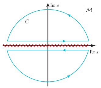
(a) Amplitude

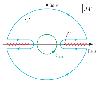
(b) Subtracted amplitude

      

Figure 1: The contour integration on the analytical $s$-plane of the amplitudes.

2.1 Subtracted Amplitude

The full amplitude is defined by the contour $C$ in Fig 1(a), which consists of an integral on discontinuities along the entire real $s$ axis, and two semi-circles at infinity which vanish because the amplitude falls fast at infinity. We divide the integral region into the infrared (IR)-region and the UV-region with separation points at $s=\Lambda^{2}$ and $s=-\Lambda^{2}$, and subtract the IR-part of this integral from the amplitude. In this way, the amplitude after subtraction will not include any singularity in the low-energy region, i.e. low energy poles and low energy branch cuts vanish in the amplitude. More precisely, we define the $M^{\prime}$ as the subtracted amplitude:

$$M^{\prime}\left(s\right) = M\left(s\right)-\frac{1}{2\pi i}\int_{-\Lambda^{2}}^{+\Lambda^{2}}{ds^{\prime}\frac{{\rm Disc}M\left(s^{\prime}\right)}{s^{\prime}-s}\ }$$ (4)

$$= \frac{1}{2\pi i}\left(\int_{-\infty}^{-\Lambda^{2}}{ds^{\prime}}+\int_{+\Lambda^{2}}^{\infty}{ds^{\prime}}\right)\frac{{\rm Disc}M\left(s^{\prime}\right)}{s^{\prime}-s}$$

$$= \frac{1}{2\pi i}\oint_{C_{\epsilon\Lambda}}{ds^{\prime}\frac{M^{\prime}\left(s^{\prime}\right)}{s^{\prime}-s}}\;.$$

In the last line we have deformed the contour $C^{\prime}$ to a small circle $C_{\epsilon\Lambda}$ by the Cauchy theorem, with $0<\epsilon<1$, see Fig. 1(b). Due to the analyticity of the subtracted amplitude inside $|s|<\Lambda^{2}$, the theory will not change when we change the radius of the dispersion relation $\epsilon\Lambda$. The $\sqrt{s}\leq\epsilon\Lambda$ is where we probe the theory and the EFT is valid inside $C_{\epsilon\Lambda}$. It can be seen from Eq.(4) that

• $M(s)$ contains singularities on the whole real $s$ axis, thus it equals to the integral on the discontinuities of $\frac{M\left(s^{\prime}\right)}{s^{\prime}-s}$ along the region $[-\infty,+\infty]$.

• $M^{\prime}\left(s\right)$ doesn’t contain any discontinuity in $[-\Lambda^{2},+\Lambda^{2}]$. We only need to integrate the interval region in which $|s|$ is greater than $\Lambda^{2}$.

It is not difficult to subtract the amplitude. We give an example for the subtraction scheme in appendix A. The result is very simple. The single pole whose location is lower than $\Lambda^{2}$, such as $\frac{1}{s-m^{2}}$ with $m^{2}<\Lambda^{2}$, will be removed from in $M(s)$ directly. Besides, the log-term $\log{(-s)}$ appearing in the loop calculation transforms as

$$\log{(-s)}\to\log{(-s)}-\frac{1}{2\pi i}\int_{0}^{\Lambda^{2}}{ds^{\prime}\frac{{\rm Disc}\log{(-s^{\prime})}}{s^{\prime}-s}\ }=\log{(\Lambda^{2}-s)}$$ (5)

where the ${\rm Disc}\log{(-s)}=-2\pi i$ have been used. This transformation can be understood as follows: the branch cut starting from the origin of real axis, after the subtraction, starts from $\Lambda^{2}$. Nevertheless, to address the IR singularities, different prescriptions have been taken in previous literatures. One can introduce a small mass $m$ for the internal propagator as a regulator Bellazzini:2020cot ; Bellazzini:2021oaj ; Arkani-Hamed:2020blm ; Chen:2022nym . However, the corresponding bounds may cause tricky problems when $m\to 0$. Alternatively, Ref Arkani-Hamed:2020blm defines the generalized effective couplings by moving the contour from origin to the complex plane. But under this circumstance, the tree-level coefficients are subdominant to terms that are generated from logarithms of loop calculations. In contrast, we will see that our prescription only produces small loop corrections to the tree-level coefficients.

Note the form of Eq.(4) is similar to that of Eq.(2). The difference is that now the contour is $C_{\epsilon\Lambda}$, in which the $M^{\prime}(s)$ is analytic. The utilization of the subtracted amplitude can make sure the effectiveness of loop calculation, and does not affect the evaluation of the integral on the UV-region. After that, we only need to prove that the second derivative of the subtracted amplitude will be constrained by the positivity bounds.

2.2 Second derivative of the subtracted amplitude

Directly taking the second derivative of Eq.(4) to $s$ we obtain

$$f^{\prime} \equiv \left.\frac{1}{2}\frac{d^{2}}{ds^{2}}M^{\prime}\left(s\right)\right|_{s\to 0}=\frac{1}{2\pi i}\oint_{C_{\epsilon\Lambda}}{ds^{\prime}\frac{M^{\prime}\left(s^{\prime}\right)}{\left(s^{\prime}\right)^{3}}}$$ (6)

$$= \frac{1}{2\pi i}\left(\int_{-\infty}^{-(\epsilon\Lambda)^{2}}{ds^{\prime}}+\int_{+(\epsilon\Lambda)^{2}}^{\infty}{ds^{\prime}}\right)\frac{{\rm Disc}M^{\prime}\left(s^{\prime}\right)}{\left(s^{\prime}\right)^{3}}$$

$$= \frac{1}{2\pi i}\left[\int_{(\epsilon\Lambda)^{2}+m^{2}}^{\infty}\frac{du\ {\rm Disc}M^{\prime}\left(m^{2}-u\right)}{\left(m^{2}-u\right)^{3}}+\int_{(\epsilon\Lambda)^{2}}^{\infty}\frac{ds^{\prime}\ {\rm Disc}M^{\prime}\left(s^{\prime}\right)}{\left(s^{\prime}\right)^{3}}\right]\;,$$

where $m^{2}$ is the sum of the squared masses of external states, and variable is changed in last line: $s^{\prime}=m^{2}-u$. Utilizing the crossing symmetry, $M_{ij\rightarrow kl}\left(s\right)=M_{i\bar{l}\rightarrow k\bar{j}}(m^{2}-s)\equiv\overline{M}_{ij\to kl}(m^{2}-s)$, where $\overline{M}$ is crossing of $M$, the ${\rm Disc}M\left(m^{2}-s\right)$ becomes

$${\rm Disc}M\left(m^{2}-s\right) \equiv M\left(m^{2}-s+i\epsilon\right)-M\left(m^{2}-s-i\epsilon\right)$$ (7)

$$= \overline{M}\left(s-i\epsilon\right)-\overline{M}\left(s+i\epsilon\right)$$

$$\equiv -{\rm Disc}\overline{M}(s)\;.$$

After that, taking the massless limit we can rewrite Eq.(6) as

$$f^{\prime} = \frac{1}{2\pi i}\int_{\left(\epsilon\Lambda\right)^{2}}^{\infty}\frac{ds^{\prime}}{\left(s^{\prime}\right)^{3}}\left[{\rm Disc}M^{\prime}\left(s^{\prime}\right)+{\rm Disc}\overline{M}^{\prime}\left(s^{\prime}\right)\right]\;.$$ (8)

By the Schwartz reflection theorem $M_{ij\rightarrow kl}\left(s+i\epsilon\right)=M_{kl\rightarrow ij}^{\ast}\left(s-i\epsilon\right)$, and the generalized optical theorem, the discontinuity of the amplitude is

$${\rm Disc}M\left(s\right) = M_{ij\rightarrow kl}\left(s+i\epsilon\right)-M_{ij\rightarrow kl}\left(s-i\epsilon\right)$$ (9)

$$= M_{ij\rightarrow kl}\left(s+i\epsilon\right)-M_{kl\rightarrow ij}^{\ast}\left(s+i\epsilon\right)$$ (10)

$$= i\sum_{X}\int{d\Pi_{X}M_{ij\rightarrow X}\left(s+i\epsilon\right)M_{kl\rightarrow X}^{\ast}(s+i\epsilon)}\;.$$ (11)

Finally, we reach the master formula as follow:

$$\left.\frac{1}{2}\frac{d^{2}M^{\prime}\left(s,t=0\right)}{ds^{2}}\right|_{s\to 0}=\sum_{X}\int_{(\epsilon\Lambda)^{2}}^{\infty}{\frac{ds^{\prime}}{2\pi\left(s^{\prime}\right)^{3}}\int d\Pi_{X}\left[M_{ij\rightarrow X}M_{kl\rightarrow X}^{\ast}+\left(j\leftrightarrow l\right)\right]}\;.$$ (12)

It should be emphasized that the traditional bound $f\geq 0$ can also be corrected at the loop level, because residues of the IR singularities are affected by loops. One may be curious for what is the difference between the traditional bound $f\geq 0$ and the subtracted bound $f^{\prime}\geq 0$. The answer is that the subtracted bound will be physically stronger than the traditional bound Bellazzini:2016xrt ; deRham:2017zjm ; deRham:2017imi . For example, we consider the forward scattering for identical particles. The traditional bound $f\geq 0$ is acquired by taking different treatments to “regulate” singularities in the IR region in the EFT Bellazzini:2020cot ; Bellazzini:2021oaj ; Arkani-Hamed:2020blm ; Chen:2022nym . By contrast, this paper directly subtract the amplitude by these singularities, i.e. $f^{\prime}=f-f_{\rm low}$, with $f_{\rm low}=\int^{\Lambda^{2}}_{0}ds^{\prime}\left[{\rm Im}{M}(s^{\prime})/s^{\prime 3}\right]\geq 0$, because the imaginary part of the forward amplitude is positive. We stress that the subtracted bound $f^{\prime}\geq 0$ is stronger since such a positive condition implies $f\geq f_{\rm low}$, which is a tighter constraint than $f\geq 0$.

With similar argument, the terms with $s$-dependence being higher than 2 in the IR amplitude can be dropped. For the quantity $f$, dropping these terms is safe, since $d^{2}(s^{n}\log(s))/ds^{2}\to 0$ as $s\to 0$ for $n>2$. However, one may find that these higher-$s$ contributions can enter the dispersion relation through $f_{\rm low}$ because they all contribute to the discontinuity. Fortunately, we will prove that higher-$s$ effects can only provide negative contributions to the bound $f^{\prime}$, and neglecting them just strengthen the bound. In this sense, we are working in a truncated EFT whose amplitude is kept up to $\mathcal{O}(s^{2})$. More explicitly, we divide the full EFT amplitude in the IR region into a truncated part and a higher-$s$ part, ${M}={M}_{\rm truncated}+{M}_{\text{higher-}s}$. The positivity condition becomes

$$f-\frac{2}{\pi}\int^{\Lambda^{2}}_{0}ds^{\prime}\frac{{\rm Im}{M}_{\rm truncated}(s^{\prime})}{s^{\prime 3}}-\frac{2}{\pi}\int^{\Lambda^{2}}_{0}ds^{\prime}\frac{{\rm Im}{M}_{\text{higher-}s}(s^{\prime})}{s^{\prime 3}}$$

$$=\sum_{X}\int_{(\epsilon\Lambda)^{2}}^{\infty}{\frac{ds^{\prime}}{\pi\left(s^{\prime}\right)^{3}}\int d\Pi_{X}\left(M_{ij\rightarrow X}M_{ij\rightarrow X}^{\ast}\right)}\geq 0\;.$$

Note that the contribution from the higher-$s$ part to the l.h.s is negative because its integral is positive. Removing this contribution from the equation will only strengthen the inequality. Therefore, it’s safe for us to neglect the higher-$s$ amplitude, as we will do in the following content.

2.3 Group theory for positivity

For the forward scattering $ij\to kl$ with $i,j,k,l$ being external states, we assume each state belongs to an irrep $\mathbf{r}$ of a symmetry groups. Two-particle states such as $\left|ij\right\rangle$ are the direct production of two irreps $\mathbf{r}_{i}$ and $\mathbf{r}_{j}$. They can be decomposed into irreps: $\mathbf{r}_{i}\otimes\mathbf{r}_{j}=\underset{\alpha}{\oplus}\ \bf{r}_{\alpha}$, where $\alpha$ is the index for inequivalent irreps. For example, in the 4-$H$ case where $H$ belongs to $\bf{2}$ of $SU(2)_{\rm L}$ symmetry, the decomposition is: $\bf{2}\otimes\bf{2}=\bf{1}\oplus\bf{3}$.

The intermediate state $\left|X\right\rangle$ can be the one-particle extension of SM at tree level, or be two-particle states at one-loop level. In either case, we can decompose the $\left|X\right\rangle$ into a sum of irreps, i.e. $\left|X\right\rangle=\sum_{\mathbf{r}_{\alpha}}C^{\mathbf{r}_{\alpha}}_{X}\left|\mathbf{r}_{\alpha}\right\rangle$. If $X$ is a one-particle state, it will be a linear combination of several irreps in which $C^{\mathbf{r}_{\alpha}}_{X}$’s are arbitrary numbers. Provided that $X$ is a two-particle state $\left|ab\right\rangle$, $C^{\mathbf{r}_{\alpha}}_{a,b}$ denotes the CG coefficients which relates the direct product of $\mathbf{r}_{a}$ and $\mathbf{r}_{b}$ with $\mathbf{r}_{\alpha}$, meanwhile the sum is a direct sum. According to this view, it is sufficient to sum over all possible irreps in Eq.(12), in which the summation becomes:

$$\sum_{\mathbf{r}_{\alpha}}{M_{ij\rightarrow\mathbf{r}_{\alpha}}M_{kl\rightarrow\mathbf{r}_{\alpha}}^{\ast}} = \sum_{\mathbf{r}_{\alpha}}{\langle kl|\mathcal{M}^{\dagger}|\mathbf{r}_{\alpha}\rangle\left\langle\mathbf{r}_{\alpha}\middle|\mathcal{M}\middle|ij\right\rangle}$$ (13)

$$= \sum_{\mathbf{r}_{\alpha}}\sum_{\mathbf{r}_{\rm in},\mathbf{r}_{\rm out}}{\left\langle kl\middle|\mathbf{r}_{\rm in}\right\rangle\langle\mathbf{r}_{\rm in}|\mathcal{M}^{\dagger}|\mathbf{r}_{\alpha}\rangle\langle\mathbf{r}_{\alpha}|\mathcal{M}|\mathbf{r}_{\rm out}\rangle\left\langle\mathbf{r}_{\rm out}\middle|ij\right\rangle}$$

$$= \sum_{\mathbf{r}_{\alpha}}{C_{i,j}^{\mathbf{r},\alpha}C_{k,l}^{\mathbf{r},\alpha\ast}\left|M_{\mathbf{r}_{\alpha}\to\mathbf{r}_{\alpha}}\right|^{2}}\;,$$

where complete sets of irreps $\mathbf{r}_{\rm in},\mathbf{r}_{\rm out}$ are inserted. The selection rule for scattering amplitude among different irreps $M_{\mathbf{r}_{\alpha}\to\mathbf{r}_{\beta}}(s,t)=\delta_{\alpha\beta}M_{\mathbf{r}_{\alpha}\to\mathbf{r}_{\alpha}}(s,t)$, which is guaranteed by the Wigner-Eckart theorem Bellazzini:2014waa , has been utilized. Substituting Eq.(13) into Eq.(12) results in

$$f^{\prime}_{ijkl}=\left.\frac{1}{2}\frac{d^{2}M_{ij\to kl}^{\prime}\left(s,t=0\right)}{ds^{2}}\right|_{s\to 0}=\int_{(\epsilon\Lambda)^{2}}^{\infty}{\frac{ds^{\prime}}{2\pi\left(s^{\prime}\right)^{3}}\sum_{\mathbf{r}_{\alpha}}{\mathcal{G}_{\mathbf{r}_{\alpha}}^{i(j|k|l)}\int d\Pi_{\mathbf{r}_{\alpha}}\left|M_{\mathbf{r}_{\alpha}\to\mathbf{r}_{\alpha}}\right|^{2}}}\;.$$ (14)

where we have defined $\mathcal{G}_{\mathbf{r}}^{ijkl}=\sum_{\alpha}C_{i,j}^{\mathbf{r},\alpha}C_{k,l}^{\mathbf{r},\alpha\ast}$, and $\mathcal{G}_{\mathbf{r}}^{i(j|k|l)}\equiv\mathcal{G}_{\mathbf{r}}^{ijkl}+\mathcal{G}_{\mathbf{r}}^{ilkj}$. In Eq.(14), the phase space integral of $|M|^{2}$ gives a cross section, thus is positive. Therefore, the $f^{\prime}_{ijkl}$ is a positive sum of $\mathcal{G}_{\mathbf{r}}^{i(j|k|l)}$, or from the geometric perspective, a convex hull formed by various $\mathcal{G}_{\mathbf{r}}^{i(j|k|l)}$. For this reason, $\mathcal{G}_{\mathbf{r}}$ is referred to as a “generator” (for a cone) Zhang:2021eeo . The $f^{\prime}_{ijkl}$ in the low-energy region can be calculated in the EFT framework, either at tree order or loop order, thus is represented as a function of Wilson coefficients. From a geometric point of view, the $\bm{f}^{\prime}$ that is viewed as a vector is constrained inside a convex cone. Normal vectors $\bm{n}$’s of the cone have positive contractions with $\bm{f}^{\prime}$, i.e. $\bm{n}\cdot\bm{f}^{\prime}\geq 0$. More precisely, these inequalities are the positivity bounds for the given function $\bm{f}^{\prime}$ of Wilson coefficients. To understand the structure of the cone and acquire it’s normal vectors, we need to explore the right hand side (r.h.s) of Eq.(14) either at tree level or loop level.

3 Tree level positivity

Positivity bounds for dim-8 coefficients of SMEFT will be derived at tree level. The function $f^{\prime}_{ijkl}$ can be viewed as a matrix with $(ij,kl)$ being the indices, whose element $f^{\prime}[ij,kl]$ indicates the value of $\frac{d^{2}}{2ds^{2}}M^{\prime}(ij\to kl)$. The general structure of this amplitude matrix, in SMEFT, can be represented by the structure of dim-8 operators. There are three dim-8 operators that are relevant for 4-$H$ scattering at tree level Li:2020gnx ; Murphy:2020rsh ; AccettulliHuber:2021uoa :

$$\mathcal{O}^{(8)}_{H1} = (D_{\mu}H^{\dagger}D_{\nu}H)(D^{\nu}H^{\dagger}D^{\mu}H)$$

$$\mathcal{O}^{(8)}_{H2} = (D_{\mu}H^{\dagger}D_{\nu}H)(D^{\mu}H^{\dagger}D^{\nu}H)$$

$$\mathcal{O}^{(8)}_{H3} = (D_{\mu}H^{\dagger}D^{\mu}H)(D_{\nu}H^{\dagger}D^{\nu}H)$$ (15)

Each operator $\mathcal{O}^{(8)}_{Hi}$ contributes to $\frac{d^{2}}{2ds^{2}}M^{\prime}(ij\to kl)$, leading to an amplitude matrix that is characterized by the $\mathbf{m}_{i}$. Due to the completeness of the operator set, any amplitude matrix $f^{\prime}_{ijkl}$ can be represented as a linear combination of the $\mathbf{m}_{i}$’s. In general, the $f^{\prime}_{ijkl}$ lives in a linear matrix space spanned by three matrices $(\mathbf{m}_{1},\mathbf{m}_{2},\mathbf{m}_{3})$. Such a space is referred to as the “amplitude space”, and $f^{\prime}_{ijkl}$ can be viewed as a vector $\bm{f}^{\prime}$ inside the space. As we have mentioned, the decomposition of the direct product for 4-$H$ process is $\bf{2}\otimes\bf{2}=\bf{1}\oplus\bf{3}$. Provided the CG coefficients for various irreps, generators are given by Refs. Zhang:2020jyn ; Zhang:2021eeo as

$$\mathcal{G}_{\mathbf{1}} =(1,0,-1),\quad\quad \mathcal{G}_{\mathbf{1}S} =(0,0,2),\quad\quad \mathcal{G}_{\mathbf{1}A} =(-2,2,0),$$

$$\mathcal{G}_{\mathbf{3}} =(0,1,0), \mathcal{G}_{\mathbf{3}S} =(4,0,-2), \mathcal{G}_{\mathbf{3}_{A}} =(2,2,-4).$$ (16)

The convex cone formed by these generators gives rise to out normal vectors as follows:

$$\bm{n}_{1}=(0,1,0),\quad\bm{n}_{2}=(1,1,0),\quad\bm{n}_{3}=(1,1,1)\;.$$ (17)

As is indicated in the Section 2.3, any amplitude $\bm{f}^{\prime}$ is constrained inside the cone by these vectors, because of $\bm{n}_{i}\cdot\bm{f}^{\prime}\geq 0$. At the tree level, only the three operators in Eq.(15) can enter the 4-$H$ process and provide $s^{2}$ terms, i.e. $\mathcal{L}_{\mathrm{int}}=\sum_{i=1}^{3}C_{Hi}^{(8)}O_{Hi}^{(8)}/\Lambda^{4}$. Under these interactions, the amplitude matrix $\bm{f}^{\prime}$ is given by

$$\Lambda^{4}\bm{f}^{\prime} = C_{H1}^{(8)}\ \mathbf{m}_{1}+C_{H2}^{(8)}\ \mathbf{m}_{2}+C_{H3}^{(8)}\ \mathbf{m}_{3}\;,$$ (18)

which can also be represented as the form of a vector $\vec{C}=(C_{H1}^{(8)},C_{H2}^{(8)},C_{H3}^{(8)})$. The normal vectors given in Eq.(17) simply produce positivity bounds as

$$C_{H2}^{(8)}\geq 0,\quad C_{H1}^{(8)}+C_{H2}^{(8)}\geq 0,\quad C_{H1}^{(8)}+C_{H2}^{(8)}+C_{H3}^{(8)}\geq 0\;,$$ (19)

which are first given in Ref. Remmen:2019cyz using the elastic approach, and are reproduced in Refs. Zhang:2020jyn ; Zhang:2021eeo based on the convex cone approach. Eq.(19) is valid at tree order, but is not necessarily correct at one-loop order.

4 Loop level positivity

4.1 Analytical bounds

At the loop level in the SMEFT, not only dim-8 operators, but also dim-4 and dim-6 operators shall enter the calculation of $\bm{f}^{\prime}$. At dim-4, the interaction is $-\lambda(H^{\dagger}H)^{2}$. And there are two operators that are directly relevant for $HH\to HH$ forward scattering at dim-6 Grzadkowski:2010es ,

$$\mathcal{O}^{(6)}_{H1} =\partial_{\mu}(H^{\dagger}H)\partial^{\mu}(H^{\dagger}H)\;,$$ (20)

$$\mathcal{O}^{(6)}_{H2} =(D_{\mu}H^{\dagger}H)(H^{\dagger}D^{\mu}H)\;.$$

The dim-6 operators that can’t appear at tree diagram but take part in the loop diagrams are divided into two types:

• $\psi^{2}H^{2}D$

  $$\mathcal{O}_{H\psi_{R}} =(H^{\dagger}i\overleftrightarrow{D}_{\mu}H)\left(\overline{\psi_{R}}\gamma^{\mu}\psi_{R}\right)\;,\quad \mathcal{O}_{Hud} =(\tilde{H}^{\dagger}iD_{\mu}H)\left(\overline{u}\gamma^{\mu}d\right)+\text{h.c. }$$

  $$\mathcal{O}_{H\psi_{L}}^{(1)} =(H^{\dagger}i\overleftrightarrow{D}_{\mu}H)\left(\overline{\psi_{L}}\gamma^{\mu}\psi_{L}\right)\;,\quad \mathcal{O}_{H\psi_{L}}^{(3)} =(H^{\dagger}i\overleftrightarrow{D}_{\mu}^{I}H)\left(\overline{\psi_{L}}\gamma^{\mu}\sigma_{I}\psi_{L}\right)\;,$$ (21)

• $X^{2}H^{2}$

  $$\mathcal{O}_{HV} =H^{\dagger}HV_{\mu\nu}V^{\mu\nu}\;,\quad \mathcal{O}_{H\widetilde{V}} =H^{\dagger}H\widetilde{V}_{\mu\nu}V^{\mu\nu}\;,$$

  $$\mathcal{O}_{HWB} =H^{\dagger}\sigma^{I}HW^{I}_{\mu\nu}B^{\mu\nu}\;,\quad \mathcal{O}_{H\widetilde{W}B} =H^{\dagger}\sigma^{I}H\widetilde{W}^{I}_{\mu\nu}B^{\mu\nu}\;,$$ (22)

where $\overleftrightarrow{D}_{\mu}\equiv\overrightarrow{D}_{\mu}-\overleftarrow{D}_{\mu}$, and $\tilde{H}=\epsilon H^{\ast}$, $\sigma^{I}$ are the Pauli matrices, $V=(B,W^{I},G^{A})$, and $\widetilde{V}_{\mu\nu}=\frac{1}{2}\varepsilon_{\mu\nu\rho\tau}V^{\rho\tau}(\varepsilon_{0123}=+1)$. However, $X^{2}H^{2}$-type operators can’t be realized by tree diagram in any UV theory, i.e. they are only obtained by UV loops. Single insertion of these operators into IR loops is suppressed by 2-loop factor $1/(16\pi^{2})^{2}$, while double insertion will be suppressed by 3-loop factor, thus they are not considered in our later discussion.

The one-loop diagrams in the SMEFT are shown in Fig. 2. The double insertions of dim-6 operators, or one dim-8 term plus one dim-4 term, can arise in loop diagrams. For simplicity, we have neglected loop diagrams consisting of couplings of SM, i.e. have taken the $g_{\rm SM}\to 0$ limit. Therefore, the loop amplitude for 4-$H$ scattering up to $\mathcal{O}(s^{2})$ has the following general form:

$$\mathcal{M}(s)\sim \Delta\lambda+(\Delta\lambda)^{2}\left(x_{1}\log\frac{\mu^{2}}{s}+x_{2}\right)$$ (23)

$$+\left[C^{(8)}_{Hi}+C^{(6)}_{i}\cdot C^{(6)}_{j}\left(y_{1}\log\frac{\mu^{2}}{s}+y_{2}\right)+\Delta\lambda\cdot C_{Hi}^{(8)}\left(z_{1}\log\frac{\mu^{2}}{s}+z_{2}\right)\right]\frac{s^{2}}{\Lambda^{4}},$$

where $\Delta\lambda$ is threshold correction to the SM coupling $\lambda$, and $(x_{i},y_{i},z_{i})$ are numbers that need to be confirmed by loop calculations. The $C^{(6)}_{i}$’s are operators listed in Eq.(20) and Eq.(21). In Eq.(23), the $C^{(6)}\cdot\lambda$ terms disappear because such terms only linearly depend on $s$, therefore can’t enter the $d^{2}\mathcal{M}/ds^{2}$.

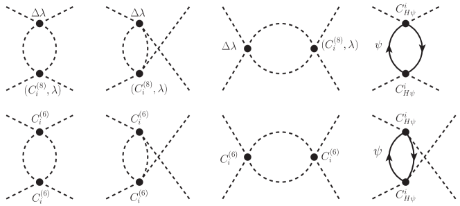
Figure 2: loop diagrams of the 4-$H$ process in EFT, the external legs are Higgs doublet, $\Delta\lambda$ is the threshold correction to SM coupling $\lambda$, meanwhile $C_{Hi}^{(8)},C_{Hi}^{(6)},C_{H\psi}^{i}$ indicate the one insertion of operators in Eq.(15), Eq.(20) and Eq.(21) respectively, the $\psi$ is the SM fermion $\psi_{L}$ or $\psi_{R}$.

We note that, thought the energy dependence of terms in the first line of Eq.(23) is shown as $s^{0}$, these terms can contribute to $d^{2}\mathcal{M}/ds^{2}|_{s\to 0}$ too, either by introducing the mass regulator Bellazzini:2020cot ; Bellazzini:2021oaj ; Arkani-Hamed:2020blm ; Chen:2022nym or defining generalized couplings Arkani-Hamed:2020blm . In the present paper, after the subtraction of the amplitude Eq.(23), log-terms in the first line also enter positivity bounds. For example, as we have indicated, the $\log{(\frac{\mu^{2}}{s})}$ will turn to be $\log{(\frac{\mu^{2}}{\Lambda^{2}+s})}$ after we adopt the subtraction. The latter one in the neighbourhood of $s=0$ is $\log{\frac{\mu^{2}}{\Lambda^{2}}}-\frac{s}{\Lambda^{2}}+\frac{s^{2}}{2\Lambda^{4}}+\mathcal{O}(s^{3})$, which can produce an $s^{2}$ term. The dim-8 operators together with the dim-4 and dim-6 operators can contribute to the amplitude space $(\mathbf{m}_{1},\mathbf{m}_{2},\mathbf{m}_{3})$ though loop diagrams in Fig. 2. According to the completeness of space, the result can be generally expanded as

$$\bm{f}^{\prime} = C^{\prime}_{1}\ \mathbf{m}_{1}+C^{\prime}_{2}\ \mathbf{m}_{2}+C^{\prime}_{3}\ \mathbf{m}_{3}\;.$$ (24)

We evaluate diagrams in Fig. 2 and give $(C^{\prime}_{1},C^{\prime}_{2},C^{\prime}_{3})$ at $\mu=\Lambda$ as follows:

$$C^{\prime}_{1}= C^{(8)}_{H1} -\frac{\Delta\lambda(36C^{(8)}_{H1}+13C^{(8)}_{H2}+13C^{(8)}_{H3}-18\Delta\lambda)}{72\pi^{2}}$$

$$+\frac{13{C^{(6)2}_{H1}}+26{C^{(6)}_{H1}}{C^{(6)}_{H2}}+8{C^{(6)2}_{H2}}-10{C^{(1)2}_{H\psi_{L}}}+10{C^{(3)2}_{H\psi_{L}}}-5C_{H\psi_{R}}^{2}+5C_{Hud}^{2}}{36\pi^{2}}\;,$$

$$C^{\prime}_{2}= C^{(8)}_{H2} -\frac{\Delta\lambda(13C^{(8)}_{H1}+36C^{(8)}_{H2}+13C^{(8)}_{H3}-18\Delta\lambda)}{72\pi^{2}}$$

$$+\frac{52{C^{(6)2}_{H1}}-52{C^{(6)}_{H1}}{C^{(6)}_{H2}}+17{C^{(6)2}_{H2}}+40{C^{(1)2}_{H\psi_{L}}}+40{C^{(3)2}_{H\psi_{L}}}+20C_{H\psi_{R}}^{2}}{144\pi^{2}}\;,$$

$$C^{\prime}_{3}= C^{(8)}_{H3} -\frac{\Delta\lambda(75C^{(8)}_{H1}+52C^{(8)}_{H2}+121C^{(8)}_{H3}-72\Delta\lambda)}{72\pi^{2}}$$ (25)

$$+\frac{56{C^{(6)}_{H1}}^{2}-26{C^{(6)}_{H1}}{C^{(6)}_{H2}}-11{C^{(6)2}_{H2}}-40C^{(3)2}_{H\psi_{L}}-10C_{Hud}^{2}}{72\pi^{2}}\;,$$

where for simplicity, we have assumed that there are only one generation and one color for fermions. In the amplitude space, the cone structure determined by generators in Eq.(16) remains unchanged. It’s normal vectors still lead to the same forms of inequalities:

$$C^{\prime}_{2}\geq 0,\quad C^{\prime}_{1}+C^{\prime}_{2}\geq 0,\quad C^{\prime}_{1}+C^{\prime}_{2}+C^{\prime}_{3}\geq 0\;,$$ (26)

Unlike Eq.(19), the $C^{\prime}_{i}$ has been modified by dim-4 and dim-6 coefficients as shown in Eq.(25), therefore inequalities in Eq.(26) are new positivity bounds at loop level.

From a top-down perspective, starting from an UV theory, Wilson coefficients can be obtained by the matching. At the one loop level, the $C_{Hi}^{(8)}=C_{Hi}^{(8)\rm tree}+C_{Hi}^{(8)\rm loop}$ in Eq.(25), where $C_{Hi}^{(8)\rm tree}$’s are the tree-matching results, and the $C_{Hi}^{(8)\rm loop}$’s are obtained through the loop-matching conditions for various UV models. Nevertheless, it’s enough to substitute rest coefficients in Eq.(25) into their tree-matching values since the coefficients are already suppressed by $\frac{1}{16\pi^{2}}$. As a result, if we keep Eq.(25) only in tree order, neglecting the terms suppressed by factor $\frac{1}{16\pi^{2}}$ will bring Eq.(26) back to the classical tree level positivity bounds. In principle, complete one-loop calculations should include those contributions from SM coupling $g_{\rm SM}$. For example, let $g_{X}$ be the coupling of the heavy particle $X$, contributions of order $\mathcal{O}(g_{\rm SM}g_{X})$ to $C^{\prime}_{i}$’s exist too. Taking into account these contributions, the final expressions of $C^{\prime}_{i}$’s will be more complex, but that don’t change the basic idea of convex cone approach. However, including terms of order $\mathcal{O}(g_{\rm SM}g_{X})$ into the positivity bounds is beyond the scope of this paper.

4.2 Discussions

Some discussions for our results are helpful. First of all, the calculation of the loop diagrams in Fig. 2 usually contains terms proportional to $s^{2}\log{(\frac{\mu^{2}}{s})}$. But, after the implementation of the subtraction scheme, such a log becomes $s^{2}\log{(\frac{\mu^{2}}{\Lambda^{2}})}+\mathcal{O}(s^{3})$, which provides contributions proportional to $\log{(\frac{\mu^{2}}{\Lambda^{2}})}$ to $C_{i}^{\prime}$’s. These contributions have been neglected in Eq.(25) by setting $\mu=\Lambda$. However, the $\mu$-dependent terms with $\log{(\frac{\mu^{2}}{\Lambda^{2}})}$ play important roles when the RG running effects on positivity bounds are considered. The RG effects are discussed in Section 5.

To test the correctness of the loop level positivity bounds, the top-down perspective will be helpful. Firstly, we find that if the heavy particle $X$ is a fermion, then $X$ can’t be the tree level completion of dim-8 operators $\mathcal{O}_{{Hi}}^{(8)}$’s, which means that $C_{Hi}^{(8)\rm tree}=0$. Except for the loop-matching coefficients $C_{Hi}^{(8)\rm loop}$, only the four $\psi^{2}H^{2}D$-type operators in Eq.(21) are possible to contribute to the amplitude $f^{\prime}$ through diagrams of fermion loop. Focusing only on $\psi^{2}H^{2}D$-type coefficients in Eq.(25), we find that positivity bounds are always satisfied if the $X$ is a fermion:

$$C^{\prime}_{2} = \frac{1}{36\pi^{2}}\left[10{C^{(1)2}_{H\psi_{L}}}+10{C^{(3)2}_{H\psi_{L}}}+5C_{H\psi_{R}}^{2}\right]\geq 0,$$

$$C^{\prime}_{1}+C^{\prime}_{2} = \frac{1}{36\pi^{2}}\left[20{C^{(3)2}_{H\psi_{L}}}+5C_{Hud}^{2}\right]\geq 0,$$

$$C^{\prime}_{1}+C^{\prime}_{2}+C^{\prime}_{3} = 0\;.$$ (27)

If the heavy particle is not a fermion, but still lead to most of tree level coefficients on r.h.s of Eq.(25) being zero, i.e. $\Delta\lambda=0$ and $C_{i}^{(n)\rm tree}=0$ for $n=6,8$, then only loop-matching coefficients $C_{Hi}^{(8)\rm loop}$’s will survive in Eq.(25). Hence, the positivity bounds in Eq.(26) must directly constrain $C^{\prime}_{i}=C_{Hi}^{(8)\rm loop}$. Some examples have illustrated such a situation, such as adding a heavy doublet with $Y=1/2$ to the SM, or the SM is extended by heavy quadruplet with $Y=1/2$ or with $Y=3/2$  Chala:2021wpj . In these three examples, as we have expected, the one-loop matching conditions do produce a set of vectors $\vec{C}^{(8)\rm loop}$ that satisfy the original tree level positivity bounds in Eq.(19).

However, if the tree level matching coefficients don’t all vanish, it is difficult to see whether Eq.(26) must be met. Thereby we should study a specific UV model and match it onto the SMEFT in the $g_{\rm SM}\to 0$ limit, to obtain the accurate values for Wilson coefficients both at tree level and loop level. Typically, if tree level coefficients $C_{Hi}^{(8)}$’s satisfy original bounds in Eq.(19) and all bounds are greater than zero, loop modifications are generally smaller than tree level coefficients, thus will not alter positiveness of bounds. However, if one of the bounds in Eq.(19) equals to zero, this bound will be dominated by $C_{Hi}^{(8)\rm loop}$ and $C_{Hi}^{(6)}$, it’s positiveness can’t be guaranteed. In such a situation, several examples are shown in the next subsection.

4.3 Examples

Some extensions of the SM have been studied for verifying the correctness of the positivity bounds. For example, we extend SM by a heavy charged triplet scalar $\Delta^{I}$ with $Y=-1$, which is the type-II seesaw model Konetschny:1977bn ; Magg:1980ut ; Schechter:1980gr ; Cheng:1980qt ; Mohapatra:1980yp ; Lazarides:1980nt . This heavy particle has brought us a non-zero vector $\vec{C}\equiv(C_{H1}^{(8)},C_{H2}^{(8)},C_{H3}^{(8)})=g_{\Delta}^{2}(0,8,0)$ at the tree level. The tree-level positivity bounds are all greater than zero:

$$C_{H2}^{(8)}=8g_{\Delta}^{2}>0,\quad C_{H1}^{(8)}+C_{H2}^{(8)}=8g_{\Delta}^{2}>0,\quad C_{H1}^{(8)}+C_{H2}^{(8)}+C_{H3}^{(8)}=8g_{\Delta}^{2}>0\;.$$ (28)

Even if we add new contributions to $\vec{C}$ from the loop level, the bounds are just slightly disturbed by the loop level coefficients, and will not be destroyed. For the same reason, most of the UV models will not break the positivity bounds at loop level. However, as Ref. Chala:2021wpj has pointed out, by the loop-matching procedure two special models may produce Wilson coefficients that violate tree level bounds in Eq.(19). So it is worthwhile to study these models again under the new bounds in this paper.

heavy neutral scalar singlet + triplet

We add a heavy neutral scalar singlet $\mathcal{S}$ and a heavy neutral scalar triplet $\Xi$ to SM at the same time, the lagrangian of interaction is written as

$$\mathcal{L}_{\rm int}=g_{\mathcal{S}}M_{\mathcal{S}}\mathcal{S}H^{\dagger}H+g_{\Xi}M_{\Xi}H^{\dagger}\Xi^{I}\sigma^{I}H\;.$$ (29)

Letting $g_{\mathcal{S}}\to 0$ or $g_{\Xi}\to 0$ converts the lagrangian to the case of one-particle extension of SM. It is reasonable to include two heavy particles because there usually can be more than one type of heavy particle existing in the loop. Sometimes one-particle extension of the SM may not be enough. For simplicity, we assume the heavy particles have same masses: $M_{\mathcal{S}}=M_{\Xi}=\Lambda$. The tree level matching gives following coefficients:

$$\Delta\lambda =\frac{-g_{\mathcal{S}}^{2}-g_{\Xi}^{2}}{2},\quad C_{H1}^{(6)\rm tree} =\frac{g_{\mathcal{S}}^{2}-g_{\Xi}^{2}}{2},\quad C_{H2}^{(6)\rm tree} =-2g_{\Xi}^{2},$$

$$C_{H1}^{(8)\rm tree} =4g_{\Xi}^{2},\quad C_{H2}^{(8)\rm tree} =0,\quad C_{H3}^{(8)\rm tree} =2g_{\mathcal{S}}^{2}-2g_{\Xi}^{2}.$$ (30)

In the meanwhile, the loop-matching dim-8 coefficients are (see appendix B for details)

$$C_{H1}^{(8)\rm loop} = -\frac{195g_{\mathcal{S}}^{4}-132g_{\mathcal{S}}^{2}g_{\Xi}^{2}+535g_{\Xi}^{4}}{720\pi^{2}},$$

$$C_{H2}^{(8)\rm loop} = -\frac{39g_{\mathcal{S}}^{4}+78g_{\mathcal{S}}^{2}g_{\Xi}^{2}+61g_{\Xi}^{4}}{144\pi^{2}},$$

$$C_{H3}^{(8)\rm loop} = -\frac{187g_{\mathcal{S}}^{4}+1386g_{\mathcal{S}}^{2}g_{\Xi}^{2}+271g_{\Xi}^{4}}{720\pi^{2}}\;,$$ (31)

in which, as we can see, $C_{H2}^{(8)\rm loop}$ is negative. It obviously destroys one of the tree level bounds in Eq.(19). However, for our improved bounds in Eq.(25), we also need to substitute the tree-matching coefficients in Eq.(30) into new bounds

$$C^{\prime}_{2} = \frac{3g_{\mathcal{S}}^{4}+6g_{\mathcal{S}}^{2}g_{\Xi}^{2}+g_{\Xi}^{4}}{48\pi^{2}}\geq 0\;$$

$$C^{\prime}_{1}+C^{\prime}_{2} = \frac{45g_{\mathcal{S}}^{4}+191g_{\mathcal{S}}^{2}g_{\Xi}^{2}+670g_{\Xi}^{4}}{360\pi^{2}}\geq 0\;,$$

$$C^{\prime}_{1}+C^{\prime}_{2}+C^{\prime}_{3} = \frac{1433g_{\mathcal{S}}^{4}+836g_{\mathcal{S}}^{2}g_{\Xi}^{2}+979g_{\Xi}^{4}}{720\pi^{2}}\geq 0\;,$$ (32)

which are also true for $g_{\mathcal{S}}\to 0$ or $g_{\Xi}\to 0$. In each limit, the loop-matching coefficients in Eq.(31) can reproduce the results of Ref. Chala:2021wpj . This example has shown that when SM is extended by neutral scalar singlet or heavy neutral scalar triplet, even if the more than one types of heavy particles run in the loop, our new positivity bounds are valid.

The type-I seesaw model

The type-I seesaw model naturally explains the tiny masses of neutrino through the seesaw mechanism Minkowski:1977sc ; Yanagida:1979as ; Gell-Mann:1979vob ; Glashow:1979nm ; Mohapatra:1979ia . This model introduces a heavy right-hand fermion singlet $N_{\rm R}$ to the SM. As we have mentioned, the case is particularly interesting when the UV particle is a fermion, because the fermion can only lead to a zero vector of $\vec{C}_{H}^{(8)}$ at the tree level. The coefficient $C_{Hi}^{(8)}$ receives contribution through the fermion loop. We find that $N_{\rm R}$ has a Yukawa interaction with the left-hand lepton doublet $\ell_{\rm L}$:

$$\mathcal{L}_{\mathrm{int}}=-\overline{\ell_{\mathrm{L}}}Y_{\nu}\widetilde{H}N_{\mathrm{R}}+\text{h.c.}\;.$$ (33)

The tree level matching of the type-I seesaw is well known, and it produces the seesaw effective field theory (SEFT) Zhang:2021tsq . SEFT-I contains a dim-5 Weinberg operator and a dim-6 operator $\mathcal{O}^{(6)}_{\rm SEFT-I}=(\overline{\ell_{\mathrm{L}}}\tilde{H})\mathrm{i}\not{\partial}(\tilde{H}^{\dagger}\ell_{\mathrm{L}})$. The Weinberg operator generates Majorana masses of neutrinos after the spontaneous gauge symmetry breaking. The dim-6 operator will cause the unitarity violation of the lepton flavor mixing matrix through modifying the normalisation of $\ell_{\rm L}$. The dim-6 operator should be rewritten in the Warsaw basis Grzadkowski:2010es :

$$\mathcal{O}^{(6)}_{\rm SEFT}=\frac{1}{4}\left[\left(\overline{\ell_{\mathrm{L}}}\gamma^{\mu}\ell_{\mathrm{L}}\right)(H^{\dagger}i\overleftrightarrow{D}_{\mu}H)-\left(\overline{\ell_{\mathrm{L}}}\gamma^{\mu}\sigma^{I}\ell_{\mathrm{L}}\right)(H^{\dagger}i\overleftrightarrow{D}_{\mu}^{I}H)\right]\;,$$ (34)

where the flavor index has been dropped since for simplicity only one generation is considered. Hence, the tree level matching coefficients that are relevant for positivity bounds are simple:

$$\Delta\lambda =0,\quad C_{H1}^{(6)\rm tree} =0,\quad C_{H2}^{(6)\rm tree} =0,$$

$$C_{H1}^{(8)\rm tree} =0,\quad C_{H2}^{(8)\rm tree} =0,\quad C_{H3}^{(8)\rm tree} =0.$$

$$C^{(1)}_{H\psi_{L}} =\frac{Y_{\nu}^{2}}{4},\quad C^{(3)}_{H\psi_{L}} =-\frac{Y_{\nu}^{2}}{4}.$$ (35)

The one-loop matching values of $C_{Hi}^{(8)}$’s are obtained by evaluating fermion loops:

$$C_{H1}^{(8)\rm loop} = \frac{Y_{\nu}^{4}}{144\pi^{2}},\quad C_{H2}^{(8)\rm loop}=\frac{59Y_{\nu}^{4}}{288\pi^{2}},\quad C_{H3}^{(8)\rm loop}=\frac{Y_{\nu}^{4}}{30\pi^{2}}\;.$$ (36)

These coefficients are all positive so tree level positivity bounds are naturally satisfied. In addition, adding the contributions from $C^{(1)}_{H\psi_{L}}$ and $C^{(3)}_{H\psi_{L}}$ does not alter the positiveness of bounds because of Eq.(27). More examples for fermion loop contributions have been considered in Ref. Zhang:2021eeo , in which the fermion loops are studied by the Cutkosky cutting rules Cutkosky:1960sp . The amplitudes from those examples are still constrained inside the convex cone, thus are allowed by positivity bounds. Under these conditions, adding the dim-6 contributions will only strengthen the bounds, as shown in Eq.(27).

5 RGE effect

In this section, we will focus on the RG running effect on the positivity bounds, i.e. explore the form of bounds at the scale $\mu<\Lambda$. For the consistency of one-loop calculations, as $\mu$ decreases, only $C_{Hi}^{(8)}$ will evolve with the scale according to it’s one-loop beta function. In Eq.(25), we don’t need to consider the RG running of dim-4 and dim-6 coefficients since they have been suppressed by the loop factor $\frac{1}{16\pi^{2}}$. In order to derive the one-loop beta function of $C_{Hi}^{(8)}$, we need to calculate the divergences of all the diagrams in Fig. 2. The exact forms of beta functions for dim-8 bosonic operators are given in Refs. Chala:2021pll ; DasBakshi:2022mwk .

In addition to the running of $C_{Hi}^{(8)}$ with the scale, we also need to consider the changes of bounds themselves with the scale. Note, we have mentioned that Eq.(25) is obtained at $\mu=\Lambda$, so the $\log{(\frac{\mu^{2}}{\Lambda^{2}})}$-dependent terms have been dropped. In consideration of the RG effect, the log-dependent terms must be put back explicitly

$$\left.C^{\prime}_{1}\right|_{\rm log} = \frac{16{C_{1}^{\left(6\right)2}}+32C_{1}^{(6)}C_{2}^{\left(6\right)}+11{C_{2}^{\left(6\right)2}}-16({C_{H\psi_{L}}^{(1)2}}-{C_{H\psi_{L}}^{(3)2}})-8({C_{H\psi_{R}}^{2}}-{C_{Hud}^{2}})}{96\pi^{2}}\log{\left(\frac{\mu^{2}}{\Lambda^{2}}\right)}\;,$$

$$\left.C^{\prime}_{2}\right|_{\rm log} = \frac{16{C_{1}^{\left(6\right)2}}-16C_{1}^{\left(6\right)}C_{2}^{\left(6\right)}+5{C_{2}^{\left(6\right)2}}+8(2{C_{H\psi_{L}}^{\left(1\right)2}}+2{C_{H\psi_{L}}^{\left(3\right)2}}+{C_{H\psi_{R}}^{2}})}{96\pi^{2}}\log{\left(\frac{\mu^{2}}{\Lambda^{2}}\right)}\;,$$

$$\left.C^{\prime}_{3}\right|_{\rm log} = \frac{40{C_{1}^{\left(6\right)2}}-16C_{1}^{\left(6\right)}C_{2}^{\left(6\right)}-7{C_{2}^{\left(6\right)2}}-8(4{C_{H\psi_{L}}^{\left(3\right)2}}+{C_{Hud}^{2}})\ }{96\pi^{2}}\log{\left(\frac{\mu^{2}}{\Lambda^{2}}\right)}\;.$$ (37)

These log-dependent terms also come from diagrams in Fig. 2, more explicitly, they are the $\log{(\frac{\mu^{2}}{s})}$’s appearing in the loop calculation. The subtraction scheme turns $\log{(\frac{\mu^{2}}{s})}$ to $\log{(\frac{\mu^{2}}{\Lambda^{2}})}+\mathcal{O}(s)$. Collecting the $\log{(\frac{\mu^{2}}{\Lambda^{2}})}$ terms brings us Eq.(37).

We find that Eq.(37) has exactly the same forms of the beta functions of $C_{Hi}^{(8)}$’s in Ref. Chala:2021pll up to an overall minus sign. This observation means that the RG evolution of $C_{Hi}^{(8)}$ is just offset by the change of the positivity bounds with the scale. Therefore, once the positivity bounds are satisfied at the scale $\mu=\Lambda$, they will be valid at any scale below $\Lambda$.

This is a general conclusion at one-loop level. Because when we calculate the beta functions of $C_{Hi}^{(8)}$’s and consider the $\mu$-dependence of bounds in Eq.(37), we are implementing the evaluation of same loop diagrams in EFT, such as Fig.2. To illustrate, we firstly denote the general expression for the running of dim-8 coefficients as: $16\pi^{2}\mu\frac{dC^{(8)}_{i}}{d\mu}=\gamma_{ij}C_{j}^{(8)}+\gamma^{\prime}_{ijk}C^{(6)}_{j}C^{(6)}_{k}$. This expression has taken into account contributions from loops involving single insertions of dimension-eight operators as well as from pairs of dimension-six operators. To determine the $\gamma$ for $C_{Hi}^{(8)}$, we calculate loops of 4-$H$ processes and give exactly the same amplitude given in Eq.(23)($g_{\rm SM}\to 0$ is taken too). After that, requiring $\mathcal{M}(s)$ is scale-independent provides that $\gamma=-32\pi^{2}z_{1}$ and $\gamma^{\prime}=-32\pi^{2}y_{1}$, where $y_{1}$’s and $z_{1}$’s are given in Eq.(37). Finally, let’s consider the effective coupling $C^{\prime}$ at an arbitrary scale $\mu$ that is below $\Lambda$:

$$C^{\prime}(\mu)=C^{(8)}_{H}(\Lambda)+\left(\frac{\gamma}{32\pi^{2}}+z_{1}\right)\log(\frac{\mu^{2}}{\Lambda^{2}})\cdot C^{(8)}_{H}+C^{(6)}\cdot\left(\frac{\gamma^{\prime}}{32\pi^{2}}+y_{1}\right)\log(\frac{\mu^{2}}{\Lambda^{2}})\cdot C^{(6)}\;,$$ (38)

where the second term and the third term vanish. Eventually, effective couolings are free of $\log(\mu)$, and positivity bounds are scale-independent.

To conclude, the RG running will not bring new physical information to positivity bounds. When we can actually measure the values of Wilson coefficients at low-energy experiments, the coefficients are determined at the characteristic scale of energy. To test the positivity, the bounds need to be modified by adding Eq.(37), and are expected to be valid at this characteristic scale.

6 Summary

In present paper, we have used the framework of convex geometry to explore the general formula for the leading $s^{2}$ positivity bounds. The formula can be applied to both the tree level and the loop level. As an explicit application, we study positivity bounds on the 4-$H$ forward scattering at the loop level. In order to remove singularities of amplitude in the IR-region without losing UV information, we have defined the subtracted amplitude. In this way, we can well handle the singularities at $s=0$ of poles and the $\log{(\frac{\mu^{2}}{s})}$-function appearing in loop calculations of EFT.

The advantage of the convex cone framework is that it uses the symmetry information of scattering particles. The matrix $f^{\prime}_{ijkl}$ in the “amplitude space” has a universal structure determined by bases of the space, regardless of whether the $f^{\prime}_{ijkl}$ is calculated by the tree diagram or the loop diagram. As long as the completeness of the dim-8 effective operator set in SMEFT Li:2020gnx ; Murphy:2020rsh is ensured, we can treat the characteristic amplitude matrices of these effective operators as bases of the amplitude space. Any $f^{\prime}_{ijkl}$ can be expanded under this group of bases. At the same time, we can calculate the generators of convex cone with CG coefficients. With the generators, the structure of the convex cone is known in the amplitude space, which will not be altered by the loop calculation. What needs to be changed is the way how the loop amplitude enters the amplitude space. The amplitude is constrained inside the convex cone, whose normal vectors correspond to positivity bounds. To conclude, positivity bounds (whether with or without the subtraction) are always the same. But when they are explained in terms of specific Wilson coefficients, they will change if loop diagrams are added.

We then use the convex cone approach to reproduce the tree level positivity bounds for 4-$H$ process, and further study the effect of loop diagrams in EFT on positivity bounds. Generally, the dim-4 and dim-6 operators will also get into the loop diagrams, hence their coefficients contribute to the amplitude space. We have obtained new positivity bounds at loop level, which have similar form to the tree level bounds. These loop bounds include small modifications to the original tree bounds. The loop modifications are all suppressed by the loop factor $\frac{1}{16\pi^{2}}$, and are induced by the dim-4 and the dim-6 operators. Neglecting these terms will bring the loop bounds back to classical tree level result. In addition, we perform the matching calculation for several special UV models to check whether the obtained loop bounds are valid. These models include the heavy neutral scalar singlet, heavy neutral scalar triplet, the type-I seesaw model and type-II seesaw model.

Finally, we investigate the influence of RGE on the positivity. Our result have shown that RG effect will not cause any violation of bounds. Besides, as long as bounds are satisfied at the cutoff (or matching) scale $\Lambda$, they will also be satisfied at any scale below $\Lambda$. This is because the new loop bounds change with the scale, and this change is just offset by the RG running of the dim-8 coefficient. The underlying physical reason is that the logarithmic terms of these two evolutions come from same loop diagrams and will cancel each other.

This work is the first to study the loop effect of leading $s^{2}$ positivity bounds in the SMEFT. Although only the forward scattering of 4-$H$ is considered, we have pointed out that the theoretical framework can be extended to other cases, such as the scattering of vector bosons or fermions. The loop effects on the bounds of these processes have not been effectively understood, and we hope to come back to these issues in the near future.

Appendix A Example of the subtraction scheme

As simple example, this appendix discusses how to subtract the singularities in low energy region from a given amplitude. Suppose that an amplitude has singularities that include a low energy pole, a high energy pole, and a branch cut from 0 to $\infty$, namely,

$$M\left(s\right)=\frac{1}{s-m^{2}}+\frac{1}{s-M^{2}}+\log{\left(-s\right)}$$ (39)

with $m^{2}<\Lambda^{2}<M^{2}$.

To subtract the low-energy singularity, we consider the contribution of an integral from the low energy region ($0<s<\Lambda^{2}$). The contour is shown in Fig. 3, where black points correspond to poles and the red cut corresponds to the branch cut of the log function. The contour contains a small circle which picks up the pole at $s^{\prime}=m^{2}$, and an integral on discontinuity of the branch cut with interval from 0 to $\Lambda^{2}$. The low-energy amplitude is given by

$$M_{\rm low}=\frac{1}{2\pi i}\left[\oint_{C}{ds^{\prime}\frac{M\left(s^{\prime}\right)}{s^{\prime}-s}}+\int_{0}^{\Lambda^{2}}{\frac{{\rm Disc}M\left(s^{\prime}\right)}{s^{\prime}-s}ds^{\prime}}\right]=\frac{-1}{m^{2}-s}-\left.\log{\left(s^{\prime}-s\right)}\right|_{0}^{\Lambda^{2}}$$ (40)

where the ${\rm Disc}\log{(-s)}=-2\pi i$ has been used. Therefore, we define the subtracted amplitude as

$$M^{\prime}\left(s\right)\equiv M\left(s\right)-M_{\rm low}=\frac{1}{s-M^{2}}+\log{\left(\Lambda^{2}-s\right)}$$ (41)

We can see that now the branch cut is starting from $s=\Lambda^{2}$, low-energy pole $s=m^{2}$ has been dropped from the subtracted amplitude, but the high-energy pole $s=M^{2}$ is left. Hence, the subtracted amplitude is totally analytical in low-energy region but it’s UV information is still kept.

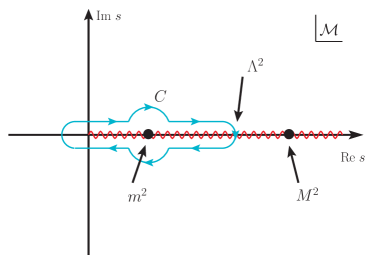
Figure 3: The contour for the amplitude in the low-energy region.

Appendix B Details of the matching procedure

We calculate two kinds of one-loop diagrams in the UV theory to obtain the one-loop matching coefficients, i.e. the one-light-particle-irreducible (1LPI) diagrams and diagrams with corrected external legs. The on-shell forward amplitude of the 1LPI diagrams are evaluated in the hard momentum region. In addition, the loop in the external leg produces a threshold correction to Higgs’s kinetic term, which contributes to dim-8 coefficients through equation of motion. Summing these two kinds of diagrams up and matching the results to the dim-8 operator bases, one-loop matching coefficients are acquired.

In our work, we evaluate the diagrams with the help of some semi-automatic programs in $\mathtt{Mathematica}$. Firstly, we use $\mathtt{FeynRules}$  Christensen:2008py to generate the $\mathtt{FeynArts}$  Hahn:2000kx model files for various models. The interface $\mathtt{FeynHelper}$  Shtabovenko:2016whf is utilized to realize the connection among $\mathtt{FeynArts}$, $\mathtt{FeynCalc}$  Shtabovenko:2016sxi and $\mathtt{Package{\text{-}}X}$  Patel:2015tea . More explicitly, $\mathtt{FeynArts}$ will provide all the Feynman diagrams and corresponding amplitudes. After that, loop integrals in the amplitudes are calculated with the help of $\mathtt{FeynCalc}$. Finally, analytical expressions for Passarino-Veltman functions  Passarino:1978jh are automatically provided by $\mathtt{Package{\text{-}}X}$.

References

- (1) T.N. Pham and T.N. Truong, Evaluation of the Derivative Quartic Terms of the Meson Chiral Lagrangian From Forward Dispersion Relation, Phys. Rev. D 31 (1985) 3027.
- (2) B. Ananthanarayan, D. Toublan and G. Wanders, Consistency of the chiral pion pion scattering amplitudes with axiomatic constraints, Phys. Rev. D 51 (1995) 1093 [hep-ph/9410302].
- (3) A. Adams, N. Arkani-Hamed, S. Dubovsky, A. Nicolis and R. Rattazzi, Causality, analyticity and an IR obstruction to UV completion, JHEP 10 (2006) 014 [hep-th/0602178].
- (4) C. de Rham, S. Melville, A.J. Tolley and S.-Y. Zhou, Positivity bounds for scalar field theories, Phys. Rev. D 96 (2017) 081702 [1702.06134].
- (5) C. de Rham, S. Melville, A.J. Tolley and S.-Y. Zhou, UV complete me: Positivity Bounds for Particles with Spin, JHEP 03 (2018) 011 [1706.02712].
- (6) N. Arkani-Hamed, T.-C. Huang and Y.-T. Huang, The EFT-Hedron, JHEP 05 (2021) 259 [2012.15849].
- (7) B. Bellazzini, J. Elias Miró, R. Rattazzi, M. Riembau and F. Riva, Positive moments for scattering amplitudes, Phys. Rev. D 104 (2021) 036006 [2011.00037].
- (8) A.J. Tolley, Z.-Y. Wang and S.-Y. Zhou, New positivity bounds from full crossing symmetry, JHEP 05 (2021) 255 [2011.02400].
- (9) S. Caron-Huot and V. Van Duong, Extremal Effective Field Theories, JHEP 05 (2021) 280 [2011.02957].
- (10) A. Sinha and A. Zahed, Crossing Symmetric Dispersion Relations in Quantum Field Theories, Phys. Rev. Lett. 126 (2021) 181601 [2012.04877].
- (11) L. Alberte, C. de Rham, S. Jaitly and A.J. Tolley, Positivity Bounds and the Massless Spin-2 Pole, Phys. Rev. D 102 (2020) 125023 [2007.12667].
- (12) C. Zhang and S.-Y. Zhou, Convex Geometry Perspective on the (Standard Model) Effective Field Theory Space, Phys. Rev. Lett. 125 (2020) 201601 [2005.03047].
- (13) X. Li, H. Xu, C. Yang, C. Zhang and S.-Y. Zhou, Positivity in Multifield Effective Field Theories, Phys. Rev. Lett. 127 (2021) 121601 [2101.01191].
- (14) L.-Y. Chiang, Y.-t. Huang, W. Li, L. Rodina and H.-C. Weng, Into the EFThedron and UV constraints from IR consistency, JHEP 03 (2022) 063 [2105.02862].
- (15) S. Caron-Huot, D. Mazac, L. Rastelli and D. Simmons-Duffin, Sharp boundaries for the swampland, JHEP 07 (2021) 110 [2102.08951].
- (16) T. Grall and S. Melville, Positivity bounds without boosts: New constraints on low energy effective field theories from the UV, Phys. Rev. D 105 (2022) L121301 [2102.05683].
- (17) Z. Bern, D. Kosmopoulos and A. Zhiboedov, Gravitational effective field theory islands, low-spin dominance, and the four-graviton amplitude, J. Phys. A 54 (2021) 344002 [2103.12728].
- (18) L. Alberte, C. de Rham, S. Jaitly and A.J. Tolley, Reverse Bootstrapping: IR Lessons for UV Physics, Phys. Rev. Lett. 128 (2022) 051602 [2111.09226].
- (19) Z.-Z. Du, C. Zhang and S.-Y. Zhou, Triple crossing positivity bounds for multi-field theories, JHEP 12 (2021) 115 [2111.01169].
- (20) B. Bellazzini, M. Riembau and F. Riva, The IR-Side of Positivity Bounds, 2112.12561.
- (21) S.D. Chowdhury, K. Ghosh, P. Haldar, P. Raman and A. Sinha, Crossing Symmetric Spinning S-matrix Bootstrap: EFT bounds, SciPost Phys. 13 (2022) 051 [2112.11755].
- (22) S. Caron-Huot, Y.-Z. Li, J. Parra-Martinez and D. Simmons-Duffin, Causality constraints on corrections to Einstein gravity, 2201.06602.
- (23) L.-Y. Chiang, Y.-t. Huang, W. Li, L. Rodina and H.-C. Weng, (Non)-projective bounds on gravitational EFT, 2201.07177.
- (24) L.-Y. Chiang, Y.-t. Huang, L. Rodina and H.-C. Weng, De-projecting the EFThedron, 2204.07140.
- (25) K. Häring and A. Zhiboedov, Gravitational Regge bounds, 2202.08280.
- (26) Y.-t. Huang and G.N. Remmen, UV-complete gravity amplitudes and the triple product, Phys. Rev. D 106 (2022) L021902 [2203.00696].
- (27) G.N. Remmen and N.L. Rodd, Spinning sum rules for the dimension-six SMEFT, JHEP 09 (2022) 030 [2206.13524].
- (28) J. Distler, B. Grinstein, R.A. Porto and I.Z. Rothstein, Falsifying Models of New Physics via WW Scattering, Phys. Rev. Lett. 98 (2007) 041601 [hep-ph/0604255].
- (29) A.V. Manohar and V. Mateu, Dispersion Relation Bounds for pi pi Scattering, Phys. Rev. D 77 (2008) 094019 [0801.3222].
- (30) B. Bellazzini, C. Cheung and G.N. Remmen, Quantum Gravity Constraints from Unitarity and Analyticity, Phys. Rev. D 93 (2016) 064076 [1509.00851].
- (31) B. Bellazzini, Softness and amplitudes’ positivity for spinning particles, JHEP 02 (2017) 034 [1605.06111].
- (32) C. Cheung and G.N. Remmen, Positive Signs in Massive Gravity, JHEP 04 (2016) 002 [1601.04068].
- (33) J. Bonifacio, K. Hinterbichler and R.A. Rosen, Positivity constraints for pseudolinear massive spin-2 and vector Galileons, Phys. Rev. D 94 (2016) 104001 [1607.06084].
- (34) C. de Rham, S. Melville, A.J. Tolley and S.-Y. Zhou, Massive Galileon Positivity Bounds, JHEP 09 (2017) 072 [1702.08577].
- (35) B. Bellazzini, F. Riva, J. Serra and F. Sgarlata, Beyond Positivity Bounds and the Fate of Massive Gravity, Phys. Rev. Lett. 120 (2018) 161101 [1710.02539].
- (36) C. de Rham, S. Melville, A.J. Tolley and S.-Y. Zhou, Positivity Bounds for Massive Spin-1 and Spin-2 Fields, JHEP 03 (2019) 182 [1804.10624].
- (37) J. Bonifacio and K. Hinterbichler, Bounds on Amplitudes in Effective Theories with Massive Spinning Particles, Phys. Rev. D 98 (2018) 045003 [1804.08686].
- (38) S. Melville and J. Noller, Positivity in the Sky: Constraining dark energy and modified gravity from the UV, Phys. Rev. D 101 (2020) 021502 [1904.05874].
- (39) C. de Rham and A.J. Tolley, Speed of gravity, Phys. Rev. D 101 (2020) 063518 [1909.00881].
- (40) L. Alberte, C. de Rham, A. Momeni, J. Rumbutis and A.J. Tolley, Positivity Constraints on Interacting Spin-2 Fields, JHEP 03 (2020) 097 [1910.11799].
- (41) M. Herrero-Valea, I. Timiryasov and A. Tokareva, To Positivity and Beyond, where Higgs-Dilaton Inflation has never gone before, JCAP 11 (2019) 042 [1905.08816].
- (42) W.-M. Chen, Y.-T. Huang, T. Noumi and C. Wen, Unitarity bounds on charged/neutral state mass ratios, Phys. Rev. D 100 (2019) 025016 [1901.11480].
- (43) L. Alberte, C. de Rham, S. Jaitly and A.J. Tolley, QED positivity bounds, Phys. Rev. D 103 (2021) 125020 [2012.05798].
- (44) Y.-t. Huang, J.-Y. Liu, L. Rodina and Y. Wang, Carving out the Space of Open-String S-matrix, JHEP 04 (2021) 195 [2008.02293].
- (45) J. Tokuda, K. Aoki and S. Hirano, Gravitational positivity bounds, JHEP 11 (2020) 054 [2007.15009].
- (46) Z.-Y. Wang, C. Zhang and S.-Y. Zhou, Generalized elastic positivity bounds on interacting massive spin-2 theories, JHEP 04 (2021) 217 [2011.05190].
- (47) Y.-J. Wang, F.-K. Guo, C. Zhang and S.-Y. Zhou, Generalized positivity bounds on chiral perturbation theory, JHEP 07 (2020) 214 [2004.03992].
- (48) M. Herrero-Valea, R. Santos-Garcia and A. Tokareva, Massless positivity in graviton exchange, Phys. Rev. D 104 (2021) 085022 [2011.11652].
- (49) C. de Rham, S. Melville and J. Noller, Positivity bounds on dark energy: when matter matters, JCAP 08 (2021) 018 [2103.06855].
- (50) D. Traykova, E. Bellini, P.G. Ferreira, C. García-García, J. Noller and M. Zumalacárregui, Theoretical priors in scalar-tensor cosmologies: Shift-symmetric Horndeski models, Phys. Rev. D 104 (2021) 083502 [2103.11195].
- (51) N. Arkani-Hamed, Y.-t. Huang, J.-Y. Liu and G.N. Remmen, Causality, unitarity, and the weak gravity conjecture, JHEP 03 (2022) 083 [2109.13937].
- (52) P. Haldar, A. Sinha and A. Zahed, Quantum field theory and the Bieberbach conjecture, SciPost Phys. 11 (2021) 002 [2103.12108].
- (53) P. Raman and A. Sinha, QFT, EFT and GFT, JHEP 12 (2021) 203 [2107.06559].
- (54) R. Gopakumar, A. Sinha and A. Zahed, Crossing Symmetric Dispersion Relations for Mellin Amplitudes, Phys. Rev. Lett. 126 (2021) 211602 [2101.09017].
- (55) M. Chala and J. Santiago, Positivity bounds in the standard model effective field theory beyond tree level, Phys. Rev. D 105 (2022) L111901 [2110.01624].
- (56) A. Zahed, Positivity and geometric function theory constraints on pion scattering, JHEP 12 (2021) 036 [2108.10355].
- (57) S. Kundu, Swampland conditions for higher derivative couplings from CFT, JHEP 01 (2022) 176 [2104.11238].
- (58) J. Davighi, S. Melville and T. You, Natural selection rules: new positivity bounds for massive spinning particles, JHEP 02 (2022) 167 [2108.06334].
- (59) A.-C. Davis and S. Melville, Scalar fields near compact objects: resummation versus UV completion, JCAP 11 (2021) 012 [2107.00010].
- (60) B. Alvarez, J. Bijnens and M. Sjö, NNLO positivity bounds on chiral perturbation theory for a general number of flavours, JHEP 03 (2022) 159 [2112.04253].
- (61) S. Melville and J. Noller, Positivity bounds from multiple vacua and their cosmological consequences, JCAP 06 (2022) 031 [2202.01222].
- (62) X. Li and S. Zhou, Origin of Neutrino Masses on the Convex Cone of Positivity Bounds, 2202.12907.
- (63) J. Henriksson, B. McPeak, F. Russo and A. Vichi, Bounding violations of the weak gravity conjecture, JHEP 08 (2022) 184 [2203.08164].
- (64) J. Albert and L. Rastelli, Bootstrapping pions at large N, JHEP 08 (2022) 151 [2203.11950].
- (65) H. Chen, A.L. Fitzpatrick and D. Karateev, Nonperturbative Bounds on Scattering of Massive Scalar Particles in , 2207.12448.
- (66) M. Carrillo Gonzalez, C. de Rham, V. Pozsgay and A.J. Tolley, Causal Effective Field Theories, 2207.03491.
- (67) C. Zhang and S.-Y. Zhou, Positivity bounds on vector boson scattering at the LHC, Phys. Rev. D 100 (2019) 095003 [1808.00010].
- (68) Q. Bi, C. Zhang and S.-Y. Zhou, Positivity constraints on aQGC: carving out the physical parameter space, JHEP 06 (2019) 137 [1902.08977].
- (69) B. Bellazzini and F. Riva, New phenomenological and theoretical perspective on anomalous ZZ and Z processes, Phys. Rev. D 98 (2018) 095021 [1806.09640].
- (70) G.N. Remmen and N.L. Rodd, Consistency of the Standard Model Effective Field Theory, JHEP 12 (2019) 032 [1908.09845].
- (71) G.N. Remmen and N.L. Rodd, Flavor Constraints from Unitarity and Analyticity, Phys. Rev. Lett. 125 (2020) 081601 [2004.02885].
- (72) S. Andriolo, T.-C. Huang, T. Noumi, H. Ooguri and G. Shiu, Duality and axionic weak gravity, Phys. Rev. D 102 (2020) 046008 [2004.13721].
- (73) M. Freytsis, S. Kumar, G.N. Remmen and N.L. Rodd, Multifield Positivity Bounds for Inflation, 2210.10791.
- (74) D. Ghosh, R. Sharma and F. Ullah, Amplitude’s positivity vs. subluminality: Causality and Unitary Constraints on dimension 6 & 8 Gluonic operators in the SMEFT, 2211.01322.
- (75) C. de Rham, L. Engelbrecht, L. Heisenberg and A. Lüscher, Positivity bounds in vector theories, 2208.12631.
- (76) B. Fuks, Y. Liu, C. Zhang and S.-Y. Zhou, Positivity in electron-positron scattering: testing the axiomatic quantum field theory principles and probing the existence of UV states, Chin. Phys. C 45 (2021) 023108 [2009.02212].
- (77) K. Yamashita, C. Zhang and S.-Y. Zhou, Elastic positivity vs extremal positivity bounds in SMEFT: a case study in transversal electroweak gauge-boson scatterings, JHEP 01 (2021) 095 [2009.04490].
- (78) J. Gu, L.-T. Wang and C. Zhang, Unambiguously Testing Positivity at Lepton Colliders, Phys. Rev. Lett. 129 (2022) 011805 [2011.03055].
- (79) C. Zhang, SMEFTs living on the edge: determining the UV theories from positivity and extremality, 2112.11665.
- (80) B. Bellazzini, L. Martucci and R. Torre, Symmetries, Sum Rules and Constraints on Effective Field Theories, JHEP 09 (2014) 100 [1405.2960].
- (81) H.-L. Li, Z. Ren, J. Shu, M.-L. Xiao, J.-H. Yu and Y.-H. Zheng, Complete set of dimension-eight operators in the standard model effective field theory, Phys. Rev. D 104 (2021) 015026 [2005.00008].
- (82) C.W. Murphy, Dimension-8 operators in the Standard Model Eective Field Theory, JHEP 10 (2020) 174 [2005.00059].
- (83) M. Accettulli Huber and S. De Angelis, Standard Model EFTs via on-shell methods, JHEP 11 (2021) 221 [2108.03669].
- (84) B. Grzadkowski, M. Iskrzynski, M. Misiak and J. Rosiek, Dimension-Six Terms in the Standard Model Lagrangian, JHEP 10 (2010) 085 [1008.4884].
- (85) W. Konetschny and W. Kummer, Nonconservation of Total Lepton Number with Scalar Bosons, Phys. Lett. B 70 (1977) 433.
- (86) M. Magg and C. Wetterich, Neutrino Mass Problem and Gauge Hierarchy, Phys. Lett. B 94 (1980) 61.
- (87) J. Schechter and J.W.F. Valle, Neutrino Masses in SU(2) x U(1) Theories, Phys. Rev. D 22 (1980) 2227.
- (88) T.P. Cheng and L.-F. Li, Neutrino Masses, Mixings and Oscillations in SU(2) x U(1) Models of Electroweak Interactions, Phys. Rev. D 22 (1980) 2860.
- (89) R.N. Mohapatra and G. Senjanovic, Neutrino Masses and Mixings in Gauge Models with Spontaneous Parity Violation, Phys. Rev. D 23 (1981) 165.
- (90) G. Lazarides, Q. Shafi and C. Wetterich, Proton Lifetime and Fermion Masses in an SO(10) Model, Nucl. Phys. B 181 (1981) 287.
- (91) P. Minkowski, at a Rate of One Out of Muon Decays?, Phys. Lett. B 67 (1977) 421.
- (92) T. Yanagida, Horizontal gauge symmetry and masses of neutrinos, Conf. Proc. C 7902131 (1979) 95.
- (93) M. Gell-Mann, P. Ramond and R. Slansky, Complex Spinors and Unified Theories, Conf. Proc. C 790927 (1979) 315 [1306.4669].
- (94) S.L. Glashow, The Future of Elementary Particle Physics, NATO Sci. Ser. B 61 (1980) 687.
- (95) R.N. Mohapatra and G. Senjanovic, Neutrino Mass and Spontaneous Parity Nonconservation, Phys. Rev. Lett. 44 (1980) 912.
- (96) D. Zhang and S. Zhou, Radiative decays of charged leptons in the seesaw effective field theory with one-loop matching, Phys. Lett. B 819 (2021) 136463 [2102.04954].
- (97) R.E. Cutkosky, Singularities and discontinuities of Feynman amplitudes, J. Math. Phys. 1 (1960) 429.
- (98) M. Chala, G. Guedes, M. Ramos and J. Santiago, Towards the renormalisation of the Standard Model effective field theory to dimension eight: Bosonic interactions I, SciPost Phys. 11 (2021) 065 [2106.05291].
- (99) S. Das Bakshi, M. Chala, A. Díaz-Carmona and G. Guedes, Towards the renormalisation of the Standard Model effective field theory to dimension eight: bosonic interactions II, Eur. Phys. J. Plus 137 (2022) 973 [2205.03301].
- (100) N.D. Christensen and C. Duhr, FeynRules - Feynman rules made easy, Comput. Phys. Commun. 180 (2009) 1614 [0806.4194].
- (101) T. Hahn, Generating Feynman diagrams and amplitudes with FeynArts 3, Comput. Phys. Commun. 140 (2001) 418 [hep-ph/0012260].
- (102) V. Shtabovenko, FeynHelpers: Connecting FeynCalc to FIRE and Package-X, Comput. Phys. Commun. 218 (2017) 48 [1611.06793].
- (103) V. Shtabovenko, R. Mertig and F. Orellana, New Developments in FeynCalc 9.0, Comput. Phys. Commun. 207 (2016) 432 [1601.01167].
- (104) H.H. Patel, Package-X: A Mathematica package for the analytic calculation of one-loop integrals, Comput. Phys. Commun. 197 (2015) 276 [1503.01469].
- (105) G. Passarino and M.J.G. Veltman, One Loop Corrections for e+ e- Annihilation Into mu+ mu- in the Weinberg Model, Nucl. Phys. B 160 (1979) 151.