On Integer Optimal Control with Total Variation Regularization on Multi-dimensional Domains

Abstract

We consider optimal control problems with integer-valued controls and a total variation regularization penalty in the objective on domains of dimension two or higher. The penalty yields that the feasible set is sequentially closed in the weak-^∗ and closed in the strict topology in the space of functions of bounded variation.

In turn, we derive first-order optimality conditions of the optimal control problem as well as trust-region subproblems with partially linearized model functions using local variations of the level sets of the feasible control functions. We also prove that a recently proposed function space trust-region algorithm—sequential linear integer programming—produces sequences of iterates whose limits are first-order optimal points.

Keywords: Mixed-integer optimal control, first-order optimality conditions, trust-region methods

AMS subject classification: 49K30,49Q15,49M05,49M37

1 Introduction

Let $\alpha>0$. Let $2\leq d\in\mathbb{N}$. Let $\Omega\subset\mathbb{R}^{d}$ be a bounded Lipschitz domain. We are concerned with optimization problems of the form

$$\begin{aligned} \min_{v\in L^{2}(\Omega)}\ &J(v)\coloneqq F(v)+\alpha\operatorname*{TV}(v)\\ \text{s.t.}\ &v(x)\in V\coloneqq\{\nu_{1},\ldots,\nu_{M}\}\subset\mathbb{Z}\text{ for almost all (a.a.)\ }x\in\Omega,\end{aligned}$$ (P)

where $F:L^{2}(\Omega)\to\mathbb{R}$ is lower semicontinuous and bounded below and $\operatorname*{TV}:L^{1}(\Omega)\to[0,\infty]$ is the total variation seminorm. Specifically, we are interested in integer optimal control problems, in which $F$ has the form $F=j\circ S$ for an objective function $j:Y\to\mathbb{R}$ and the (potentially non-linear) solution operator $S:L^{2}(\Omega)\to Y$ of a PDE (or $S$ is another kind of integral operator) with state space $Y$. The distinctive feature of (P) is the integrality constraint on the control $v$.

Integer optimal control problems are a versatile mathematical problem class that allows for modeling many scenarios with real world applications, for example, transmission line control [13], traffic light control [14], gas network control [34, 19], and automotive control [12]. Owing to these applications, integer optimal control has attracted significant interest in recent years. We highlight the research on the combinatorial integral approximation [42, 20, 41, 32, 23, 18], which is closely related to relaxation-based approaches in shape and topology optimization [1, 45] and compensated compactness [47]. Recently, descent optimization algorithms that produce integer-valued controls directly without solving the relaxation have also been investigated, see, for example, [17, 49]. They are based on the same principles as the combinatorial integral approximation, which is shown in [31]. The aforementioned results can provide optimal approximation guarantees on the computed integer-valued control functions, for the case $\alpha=0$, where no regularization is present. In [30] it has been shown that the convex relaxation of a so-called multi-bang regularizer [7, 8] may be integrated into the combinatorial integral approximation.

However, without enforcing more regularity on the control input $v$ in (P) these approaches lead to approximations of functions with convex codomains in weak topologies of $L^{p}$ spaces, see also the Lyapunov convexity theorem [28, 26], which means that close approximations may exhibit highly oscillating functions with their total variation tending towards infinity [20]. While the approximation algorithms that compute the integer controls have been tailored to reduce oscillations [3, 43] this effect is inevitable.

Therefore, it has been proposed to enforce control functions of bounded variation by choosing $\alpha>0$ in [25]. Driven by applications in mathematical imaging, total variation regularization has been analyzed in depth, see [39, 48, 10, 6, 5, 24, 21], and also entered research on optimal control problems, see [27, 22, 11, 16]. Combining $\alpha>0$ with the integrality constraint $v(x)\in V$ a.e., it follows that the feasible set of (P) is sequentially weak-^∗ closed in the space of functions of bounded variation. Thus (P) admits a solution in this setting, see, e.g., the analysis in [2, Chap. 4-5], [4, Cor. 2.6], or [25, Prop. 2.3].

Because of the sequential weak-^∗ closedness of the feasible set, a novel trust-region algorithm that operates on the feasible set is proposed in [25]. The model function of the trust-region subproblems is the sum of a linearization of $F$ and the term $\alpha\operatorname*{TV}$, meaning that the latter is kept exactly. The trust region is an $L^{1}$-ball around the current iterate. After discretization, this leads to linear integer programs. Optimality conditions for (P) and asymptotics of the trust-region algorithm have been analyzed for the case $d=1$, that is if $\Omega$ is an open interval. For this case, the trust-region subproblems can be solved efficiently with the strategies proposed in [44, 33] and it has been noted in [25] that when the sequence of heights of the steps of the control function settles during the optimization procedure, optimizing (P) becomes a switching point optimization, for which optimization techniques have been investigated [40, 9, 35, 46]. A proximal objective instead of a trust-region globalization has been proposed in [33].

None of these works has addressed the case that the domain is multi-dimensional, that is $d\geq 2$, where the geometric properties of the $\operatorname*{TV}$-term differ fundamentally from $d=1$, however. This work closes this gap.

Contribution

We analyze optimality conditions for (P) and the function space algorithm from [25] for the case $d\geq 2$. In particular, we employ and extend results on geometric variational problems to derive first-order optimality conditions for (P) and trust-region subproblems using so-called local variations. The underlying variational principle gives rise to a sufficient decrease condition (related to Cauchy point computations in nonlinear programming). We leverage this insight to prove convergence of the trust-region algorithm to first-order optimal points.

As an intermediate result, we verify $\Gamma$-convergence, more specifically the $\liminf$- and $\limsup$-inequalities for the trust-region subproblems with respect to convergence of the (partial) linearization point for the subproblem. Notably, this result is not true for $d=1$ but opens possibilities for algorithmic improvements, in particular, sources of inexactness in the trust-region subproblems.

While rigorous numerical analysis and computational assessment are not our focus and beyond the scope of this article, we nevertheless provide first computational experiments in Section 7 to allow some impression on the algorithm in practice.

Structure of the remainder

We introduce some notation and functions of bounded variation in Section 2 followed by local variations and preparations in Section 3. We define locally optimal solutions and prove a first-order optimality condition for (P) in Section 4. We define and analyze the trust-region subproblems and introduce the algorithm in Section 5. Then we derive our variational stationarity concept and prove the convergence of the iterates of the trust-region algorithm to stationary points in Section 6. We provide computational experiments in Section 7 and concluding remarks in Section 8.

2 Notation and Primer on Functions of Bounded Variation

The symmetric difference of the sets $A$, $B\subset\mathbb{R}^{d}$ is $A\Delta B$. The Lebesgue measure is denoted by $\lambda$. The restriction of a measure $\mu$ to a set $A$ is denoted by $\mu\mathbin{\vrule height=6.88889pt,depth=0.0pt,width=0.55974pt\vrule height=0.55974pt,depth=0.0pt,width=5.59721pt}A$. For a Lebesgue space $L^{p}(\Omega)$ on $\Omega$, we abbreviate $\|\cdot\|_{L^{p}(\Omega)}$ by $\|\cdot\|_{L^{p}}$. We abbreviate the $L^{2}(\Omega)$-inner product by $(\cdot,\cdot)_{L^{2}}$. The $\{0,1\}$-valued indicator function of a set $A$ is $\chi_{A}$. Let $E\subset\Omega$ be measurable. We define the perimeter of $E$ in $\Omega$, see, e.g, [2, Def. 3.35], as

$$P(E,\Omega)\coloneqq\sup\left\{\int_{E}\operatorname*{div}\varphi(x)\mathop{}\!\mathrm{d}x\,\Big{|}\,\varphi\in(C_{c}^{1}(\Omega))^{d}\text{ and }\sup_{x\in\Omega}\|\varphi(x)\|\leq 1\right\}.$$

If $P(E,\Omega)<\infty$, $E$ is called a Caccioppoli set. A partition $\{E_{i}\}_{i\in I}$ of $\Omega$ is called a Caccioppoli partition if $\sum_{i\in I}P(E_{i},\Omega)<\infty$. We denote the topological boundary of $E$ by $\partial E$ and the reduced boundary of $E$ by $\partial^{*}E$, see [2, Def. 3.54]. We denote the essential boundary, the set of points that have neither density $1$ nor $0$ with respect to $A$, see [2, Def. 3.54], by $\partial^{e}A$. Note that $\partial^{*}E$ may intersect with $\partial^{*}\Omega$ so that $P(E,\Omega)=\mathcal{H}^{d-1}(\partial^{*}E\cap\Omega)$ while $P(E,\Omega)\neq\mathcal{H}^{d-1}(\partial^{*}E)$. We recall that a function $u\in L^{1}(\Omega)$ is of bounded variation (in $\operatorname*{BV}(\Omega)$) if its distributional derivative $Du$ is a finite Radon measure in $\Omega$ [2, Chap. 3]. In other words $\operatorname*{TV}(u)\coloneqq|Du|(\Omega)<\infty$, where $|\mu|$ denotes the total variation measure of a measure $\mu$. Most notably $\operatorname*{TV}(\chi_{E})=P(E,\Omega)$ for a Borel set $E\subset\Omega$. A sequence of functions $(v^{n})_{n}\subset\operatorname*{BV}(\Omega)$ converges weakly-^∗ to $v\in\operatorname*{BV}(v)$, denoted by $v^{n}\stackrel{{\scriptstyle\ast}}{{\rightharpoonup}}v$, if $v^{n}\to v$ in $L^{1}(\Omega)$ and $\limsup_{n\to\infty}\operatorname*{TV}(v^{n})<\infty$. Moreover, $(v^{n})_{n}$ converges strictly to $v\in\operatorname*{BV}(v)$ if $v^{n}\to v$ in $L^{1}(\Omega)$ and $\operatorname*{TV}(v^{n})\to\operatorname*{TV}(v)<\infty$.

Feasible points for (P) are functions in $\operatorname*{BV}(\Omega)$ that attain values only in the finite set $V$. Their distributional derivatives are absolutely continuous with respect to $\mathcal{H}^{d-1}$ [2, Theorems 3.36 and 3.59]. In particular, they are also so-called $SBV$-functions ($S$ for Special), see [2, Sec. 4.1]. We define

$$\operatorname*{BV_{V}}(\Omega)\coloneqq\left\{v\in\operatorname*{BV}(\Omega)\,|\,v(x)\in V\text{ for a.a.\ }x\in\Omega\right\}\subset\operatorname*{BV}(\Omega),$$

which is the feasible set of (P). We will use the following lemma (proven in Appendix A).

Lemma 2.1.

1. $\operatorname*{BV_{V}}(\Omega)$ is sequentially weakly-^∗ and strictly closed in $\operatorname*{BV}(\Omega)$.

2. Let $v\in\operatorname*{BV_{V}}(\Omega)$. Then there exists a Caccioppoli partition $\{E_{1},\ldots,E_{M}\}$ of $\Omega$ such that $v=\sum_{i=1}^{M}\nu_{i}\chi_{E_{i}}$.

3. Let $\sum_{i=1}^{M}\nu_{i}\chi_{E_{i}}=v\in\operatorname*{BV}_{V}(\Omega)$ as in (b). Then it holds that

   $$\infty>\operatorname*{TV}(v) =|Dv|(\Omega)=\sum_{i=1}^{M-1}\sum_{j=i+1}^{M}|\nu_{i}-\nu_{j}|\mathcal{H}^{d-1}(\partial^{*}E_{i}\cap\partial^{*}E_{j})\text{ and}$$ (1)

   $$\operatorname*{TV}(v) \geq\frac{1}{2}\sum_{i=1}^{M}P(E_{i},\Omega).$$ (2)

3 Local Variations

A key concept to derive sensible notions of stationarity for (P) and subsequently a sufficient decrease condition for our algorithmic framework are local variations, which allow to analyze smooth perturbations of the boundaries of the level sets of feasible control functions. We introduce the relevant concepts leaning on [29].

Definition 3.1.

1. A one parameter family of diffeomorphisms of $\mathbb{R}^{d}$ is a smooth function $f:(-\varepsilon,\varepsilon)\times\mathbb{R}^{d}\to\mathbb{R}^{d}$ for some $\varepsilon>0$ such that for all $t\in(-\varepsilon,\varepsilon)$, the function $f_{t}(\cdot)\coloneqq f(t,\cdot):\mathbb{R}^{d}\to\mathbb{R}^{d}$ is a diffeomorphism.

2. Let $A\subset\mathbb{R}^{d}$ be open. Then the family $(f_{t})_{t\in(-\varepsilon,\varepsilon)}$ is a local variation in $A$ if additionally to (a) we have $f_{0}(x)=x$ for all $x\in\mathbb{R}^{d}$ and there is a compact set $K\subset A$ such that $\{x\in\mathbb{R}^{d}\,|\,f_{t}(x)\neq x\}\subset K$ for all $t\in(-\varepsilon,\varepsilon)$.

3. For a local variation, we define its initial velocity: $\phi(x)\coloneqq\frac{\partial f}{\partial t}(0,x)$ for $x\in\mathbb{R}^{d}$.

We recall basic properties and a certain local variation that is important in the remainder.

Proposition 3.2.

Let $\phi\in C_{c}^{\infty}(\Omega,\mathbb{R}^{d})$. Let $f_{t}\coloneqq I+t\phi$ for $t\in\mathbb{R}$. Then $(f_{t})_{t\in(-\varepsilon,\varepsilon)}$ is a local variation in $\Omega$ with initial velocity $\phi$ for some $\varepsilon>0$.

Proof.

Because of $\|\nabla f_{t}(x)-I\|=\|t\nabla\phi(x)\|=|t|\|\nabla\phi(x)\|\leq|t|M$ with $M\coloneqq\max_{x\in\bar{\Omega}}\|\nabla\phi(x)\|<\infty$, Lemma A.1 yields the existence of some $\varepsilon>0$ such that $(f_{t})_{t\in(-\varepsilon,\varepsilon)}$ is a one parameter family of diffeomorphisms. We have $f_{0}(x)=x$ for all $x\in\mathbb{R}^{d}$ and $\{x\in\mathbb{R}^{d}|f_{t}(x)\neq x\}\subset\operatorname*{supp}\phi\subset\Omega$ for all $t\in\mathbb{R}$. Hence, $(f_{t})_{t\in(-\varepsilon,\varepsilon)}$ is a local variation in $\Omega$ with initial velocity $\frac{\partial f}{\partial t}(0,x)=\phi(x)$ for $x\in\mathbb{R}^{d}$. ∎

Let $v=\sum_{i=1}^{M}\nu_{i}\chi_{E_{i}}$ for a Caccioppoli partition $\{E_{1},\ldots,E_{M}\}$ of $\Omega$. Let $(f_{t})_{t\in(-\varepsilon,\varepsilon)}$ be a local variation in $\Omega$ with initial velocity $\phi$. Because the $f_{t}$ are diffeomorphisms it follows that $\{f_{t}(E_{1}),\ldots,f_{t}(E_{M})\}$ is a partition of $\Omega$ that induces the piecewise constant function

$$f_{t}^{\#}v\coloneqq\sum_{i=1}^{M}\nu_{i}\chi_{f_{t}(E_{i})}.$$

For a $C_{c}^{\infty}(\Omega;\mathbb{R}^{d})$-function $\phi$ we introduce the notation $\operatorname*{div}{}_{E}\phi:\partial^{*}E\to\mathbb{R}$ for the so-called boundary divergence of $\phi$ on $E$,

$$\operatorname*{div}{}_{E}\phi(x)\coloneqq\operatorname*{div}\phi(x)-n_{E}(x)\cdot\nabla\phi(x)n_{E}(x),$$

where $n_{E}$ denotes the unit outer normal vector on the reduced boundary of $E$. We obtain Taylor expansions for $(g,f^{\#}_{t}v)_{L^{2}}$ and $\operatorname*{TV}(f^{\#}_{t}v)$ with respect to $t$, which we prove below.

Lemma 3.3 (Extension of Theorem 17.5 in [29]).

Let $\{E_{1},\ldots,E_{M}\}$ be a Caccioppoli partition of $\Omega$, and $v=\sum_{i=1}^{M}\nu_{i}\chi_{E_{i}}$. Let $(f_{t})_{t\in(-\varepsilon,\varepsilon)}$ be a local variation in $\Omega$ with initial velocity $\phi$. Then there exists $\varepsilon_{0}>0$ such that

$$\operatorname*{TV}(f_{t}^{\#}v)=\operatorname*{TV}(v)+t\sum_{i=1}^{M}\sum_{j=i+1}^{M}|\nu_{i}-\nu_{j}|\int_{\partial^{*}E_{i}\cap\partial^{*}E_{j}}\operatorname*{div}{}_{E_{i}}\phi(x)\mathop{}\!\mathrm{d}\mathcal{H}^{d-1}(x)+O(t^{2})$$

for all $t\in(-\varepsilon_{0},\varepsilon_{0})$.

Proof.

The claim follows with the identities

$$\operatorname*{TV}(f_{t}^{\#}v)$$

$$=\sum_{i=1}^{M}\sum_{j=i+1}^{M}|\nu_{i}-\nu_{j}|\mathcal{H}^{d-1}(\partial^{*}f_{t}(E_{i})\cap\partial^{*}f_{t}(E_{j}))$$

$$=\sum_{i=1}^{M}\sum_{j=i+1}^{M}|\nu_{i}-\nu_{j}|\mathcal{H}^{d-1}(\partial^{*}f_{t}(E_{i})\cap f_{t}(\partial^{*}E_{j}))$$

$$=\sum_{i=1}^{M}\sum_{j=i+1}^{M}|\nu_{i}-\nu_{j}|\int_{\partial^{*}E_{i}\cap\partial^{*}E_{j}}\mathcal{J}_{x}f_{t}(x)\|((\nabla f^{-1}_{t}\circ f_{t})(x))^{T}n_{E_{i}}(x)\|\mathop{}\!\mathrm{d}\mathcal{H}^{d-1}(x)$$

$$=\sum_{i=1}^{M}\sum_{j=i+1}^{M}|\nu_{i}-\nu_{j}|\int_{\partial^{*}{E_{i}}\cap\partial^{*}E_{j}}(1+t\operatorname*{div}{}_{E_{i}}\phi(x))\mathop{}\!\mathrm{d}\mathcal{H}^{d-1}(x)+O(t^{2})$$

$$=\operatorname*{TV}(v)+t\sum_{i=1}^{M}\sum_{j=i+1}^{M}|\nu_{i}-\nu_{j}|\int_{\partial^{*}E_{i}\cap\partial^{*}E_{j}}\operatorname*{div}{}_{E_{i}}\phi(x)\mathop{}\!\mathrm{d}\mathcal{H}^{d-1}(x)+O(t^{2})$$

that are due to (in the order of their appearance): (1), Prop. 17.1 (17.4) in [29], Prop. 17.1 (17.6) in [29], the proof of Thm 17.5 in [29], and (1). Note that $\mathcal{J}_{x}f_{t}$ denotes the Jacobian determinant of the function $f_{t}$. ∎

Corollary 3.4.

Let $\{E_{1},\ldots,E_{M}\}$ be a Caccioppoli partition of $\Omega$, Let $(f_{t})_{t\in(-\varepsilon,\varepsilon)}$ be a local variation with initial velocity $\phi\in C_{c}^{\infty}(\Omega;\mathbb{R}^{d})$. Then there exists $\varepsilon_{0}>0$ such that the partition $\{f_{t}(E_{1}),\ldots,f_{t}(E_{M})\}$ is a Caccioppoli partition for all $t\in(-\varepsilon_{0},\varepsilon_{0})$.

Proof.

The claim follows from Lemma 3.3 and (1). ∎

Lemma 3.5 (Extension of Proposition 17.8 in [29]).

Let $(f_{t})_{t\in(-\varepsilon,\varepsilon)}$ be a local variation with initial velocity $\phi\in C_{c}^{\infty}(\Omega;\mathbb{R}^{d})$. Let $g\in C(\bar{\Omega})$. Then it follows that

$$\int_{\Omega}g(x)(f_{t}^{\#}v(x)-v(x))\mathop{}\!\mathrm{d}x=t\sum_{i=1}^{M}\nu_{i}\int_{\partial^{*}E_{i}\cap\Omega}g(x)\left(\phi(x)\cdot n_{E_{i}}(x)\right)\mathop{}\!\mathrm{d}\mathcal{H}^{d-1}(x)+o(t).$$

Proof.

The claim follows from the following identities, where the second is due to Proposition 17.8 in Section 17.3 in [29]:

$$\int_{\Omega}g(x)(f_{t}^{\#}v(x)-v(x))\,\mathop{}\!\mathrm{d}x =\sum_{i=1}^{M}\nu_{i}\int_{\Omega}g(x)(\chi_{f_{t}(E_{i})}(x)-\chi_{E_{i}}(x))\,\mathop{}\!\mathrm{d}x$$

$$=t\sum_{i=1}^{M}\nu_{i}\int_{\partial^{*}E_{i}\cap\Omega}g(x)\left(\phi(x)\cdot n_{E_{i}}(x)\right)\mathop{}\!\mathrm{d}\mathcal{H}^{d-1}(x)+o(t).$$

∎

If a local variation $(f_{t})_{t\in(-\varepsilon,\varepsilon)}$ is given as in Proposition 3.2, we can obtain Lipschitz continuity for the measure of the intersection of a Caccioppoli set $F$ and a transformed Caccioppoli set $f_{t}(E)$.

Lemma 3.6.

Let $\phi\in C_{c}^{\infty}(\Omega;\mathbb{R}^{d})$. Let $(f_{t})_{t\in(-\varepsilon,\varepsilon)}$ be the local variation defined by $f_{t}\coloneqq I+t\phi$ for $t\in(-\varepsilon,\varepsilon)$. Then there exist $0<\varepsilon_{0}<\varepsilon$ and $L>0$ such that for all $s$, $t\in(-\varepsilon_{0},\varepsilon_{0})$ and all Caccioppoli sets $E$, $F$ in $\Omega$ it holds that

$$\left|\lambda(f_{t}(E)\cap F)-\lambda(f_{s}(E)\cap F)\right|\leq L|t-s|P(E,\Omega).$$

Proof.

We adapt the strategy of the proof of Lemma 17.9 in [29] that shows the bound $\lambda(f_{t}(E)\Delta E)\leq L|t|\operatorname*{TV}(\chi_{E})$. Let $g_{t}\coloneqq f_{t}^{-1}$ for all $t\in(-\varepsilon,\varepsilon)$. Let $s$, $t\in(-\varepsilon,\varepsilon)$ be given. We define $u_{\delta}\in\operatorname*{BV}(\Omega)\cap C^{\infty}(\Omega)$ as in [evans2015measure, Thm. 5.3] so that

$$u_{\delta}\to\chi_{E}\text{ in }L^{1}(\Omega)\enskip\text{and}\enskip\int_{\Omega}\|\nabla u_{\delta}(x)\|\mathop{}\!\mathrm{d}x=|Du_{\delta}|(\Omega)\to|D\chi_{E}|(\Omega)\enskip\text{as}\enskip\delta\to 0.$$ (3)

This implies

$$\left|\lambda(f_{t}(E)\cap F)-\lambda(f_{s}(E)\cap F)\right| =\left|\int_{F}|\chi_{E}(g_{t}(x))|\mathop{}\!\mathrm{d}x-\int_{F}|\chi_{E}(g_{s}(x))|\mathop{}\!\mathrm{d}x\right|$$

$$\leq\int_{F}|\chi_{E}(g_{t}(x))-\chi_{E}(g_{s}(x))|\mathop{}\!\mathrm{d}x$$ (4)

$$=\lim_{\delta\to 0}\int_{F}|u_{\delta}(g_{t}(x))-u_{\delta}(g_{s}(x))|\mathop{}\!\mathrm{d}x,$$

where we have used the reverse triangle inequality to obtain the inequality. Before we continue to analyze the right hand side of this estimate, we need some preparations.

We define $G_{t,s,\alpha}(x)\coloneqq\alpha g_{t}(x)+(1-\alpha)g_{s}(x)$ for $\alpha\in[0,1]$ and $x\in\mathbb{R}^{d}$. For the derivative of $G_{t,s,\alpha}(x)$ with respect to $\alpha$, we obtain

$$\frac{\partial}{\partial\alpha}G_{t,s,\alpha}(x)=g_{t}(x)-g_{s}(x).$$

For all (arbitrary but fixed) $\alpha\in[0,1]$, we compute the Jacobian determinant of $G_{t,s,\alpha}(x)$ with respect to $x$ and obtain

$$\mathcal{J}_{x}G_{t,s,\alpha}(x)=\sqrt{\det\left((\alpha\nabla g_{t}(x)+(1-\alpha)\nabla g_{s}(x))(\alpha\nabla g_{t}(x)+(1-\alpha)\nabla g_{s}(x))^{T}\right).}$$

Lemma A.2 gives $\nabla g_{\tau}(x)\to I$ for $\tau\to 0$ uniformly for $x\in\mathbb{R}^{d}$. Consequently, we obtain uniformly for all $x\in\mathbb{R}^{d}$ that

$$\|I-\nabla G_{s,t,\alpha}(x)\|\leq\alpha\|I-\nabla g_{s}(x)\|+(1-\alpha)\|I-\nabla g_{t}(x)\|\eqqcolon\delta,$$

where $\delta$ can be made arbitrarily small also uniformly for $\alpha\in[0,1]$ by only allowing sufficiently small absolute values for $s$ and $t$. Thus by virtue of Lemma A.1 there exists $\varepsilon_{0}>0$ such that the function $G_{s,t,\alpha}$ is invertible for all $s$, $t\in(-\varepsilon_{0},\varepsilon_{0})$ and all $\alpha\in[0,1]$. Moreover, after possibly reducing $\varepsilon_{0}$ further, we obtain for all $s$, $t\in(-\varepsilon_{0},\varepsilon_{0})$ and all $x\in\mathbb{R}^{d}$ that

$$\mathcal{J}_{x}G_{t,s,\alpha}(x)\geq 0.5.$$ (5)

We continue our analysis of $d_{\delta}\coloneqq\int_{F}|u_{\delta}(g_{t}(x))-u_{\delta}(g_{s}(x))|\mathop{}\!\mathrm{d}x$ and deduce

$$d_{\delta} =\int_{F}|u_{\delta}(G_{t,s,1}(x))-u_{\delta}(G_{t,s,0}(x))|\mathop{}\!\mathrm{d}x G_{s,t,\alpha}(x)$$ Definition of

$$=\int_{F}\left|\int_{0}^{1}\frac{\partial}{\partial\alpha}u_{\delta}(G_{t,s,\alpha}(x))\Big{|}_{\alpha=\beta}\mathop{}\!\mathrm{d}\beta\right|\mathop{}\!\mathrm{d}x$$ Fundamental theorem of calculus

$$\leq\int_{F}\int_{0}^{1}\left\|\nabla u_{\delta}(G_{t,s,\alpha}(x))\right\|\mathop{}\!\mathrm{d}\alpha\left\|g_{t}(x)-g_{s}(x)\right\|\mathop{}\!\mathrm{d}x.$$ Chain rule and submultiplicativity

By Lemma A.2 there exists $C_{2}>0$ such that $\left\|g_{t}(x)-g_{s}(x)\right\|\leq C_{2}|t-s|$. We insert this inequality and apply Fubini’s theorem to obtain the estimate

$$d_{\delta}\leq C_{2}|t-s|\int_{0}^{1}\int_{F}\left\|\nabla u_{\delta}(G_{t,s,\alpha}(x))\right\|\mathop{}\!\mathrm{d}x\mathop{}\!\mathrm{d}\alpha.$$ (6)

Next, we observe

$$G_{t,s,\alpha}(\Omega)=\Omega$$ (7)

To see this, we note that if $x\notin\operatorname*{supp}\phi$, then $x=G_{t,s,\alpha}(x)$. Combining this with $\operatorname*{supp}\phi\subset\Omega$, we obtain $G_{s,t,\alpha}(\Omega)=\Omega$ because $G_{s,t,\alpha}$ is invertible for all $s$, $t\in(-\varepsilon_{0},\varepsilon_{0})$ and all $\alpha\in[0,1]$. We apply the change of variables formula and the inverse function theorem to obtain

$$\int_{F}\left\|\nabla u_{\delta}(G_{t,s,\alpha}(x))\right\|\mathop{}\!\mathrm{d}x =\int_{F}\frac{\left\|\nabla u_{\delta}(G_{t,s,\alpha}(x))\right\|}{\mathcal{J}_{x}G_{t,s,\alpha}(x)}\mathcal{J}_{x}G_{t,s,\alpha}(x)\mathop{}\!\mathrm{d}x \cdot 1$$

$$=\int_{G_{t,s,\alpha}(F)}\frac{\left\|\nabla u_{\delta}(y)\right\|}{\mathcal{J}_{x}G_{t,s,\alpha}(G_{t,s,\alpha}^{-1}(y))}\mathop{}\!\mathrm{d}y$$ Area formula

$$\leq 2\int_{\Omega}\left\|\nabla u_{\delta}(y)\right\|\mathop{}\!\mathrm{d}y.$$ (5), (7) (8)

We insert the estimate (8) into (6) and pass to the limit $\delta\to 0$, which gives

$$d_{\delta}\leq 2C_{2}\int_{\Omega}\|\nabla u_{\delta}(y)\|\mathop{}\!\mathrm{d}y|t-s|\,\underset{\eqref{eq:partition_of_unity}}{\to}2C_{2}|D\chi_{E}|(\Omega)|t-s|=\,2C_{2}P(E,\Omega)|t-s|.$$

The claim follows by combining these considerations with the estimate $|\lambda(f_{t}(E)\cap F)-\lambda(f_{s}(E)\cap F)|\leq\lim_{\delta\to 0}d_{\delta}$ and the choice $L\coloneqq 2C_{2}$. ∎

Remark 3.7.

From the proof of Lemma 3.6 it can also be derived that

$$\lambda(f_{t}(E)\Delta f_{s}(E))\leq L|t-s|P(E,\Omega)$$

by using that $\lambda(f_{t}(E)\Delta f_{s}(E))=\int_{\Omega}|\chi_{E}(g_{t}(x))-\chi_{E}(g_{s}(x))|\mathop{}\!\mathrm{d}x$ and continuing the proof from (4) with the choice $F=\Omega$.

Lemma 3.6 implies the following lemma, which will be useful in the remainder.

Lemma 3.8.

Let $\{E_{1},\ldots,E_{M}\}$ be a Caccioppoli partition of $\Omega$ and $v=\sum_{i=1}^{M}\nu_{i}\chi_{E_{i}}$. Let $(f_{t})_{t\in(-\varepsilon,\varepsilon)}$ be the local variation defined by $f_{t}\coloneqq I+t\phi$ with $\phi\in C_{c}^{\infty}(\Omega,\mathbb{R}^{d})$. Then there exist $\varepsilon_{0}>0$ and $C>0$ such that for all $t\in(-\varepsilon_{0},\varepsilon_{0})$ it holds that

$$\|f_{t}{{}^{\#}}v-v\|_{L^{1}}\leq C|t|.$$

Proof.

Lemma 3.6 gives $L>0$ and $\varepsilon_{0}>0$ such that

$$\lambda(f_{t}(E_{i})\cap E_{j})=\lambda(f_{t}(E_{i})\cap E_{j})-\lambda(f_{0}(E_{i})\cap E_{j})\leq L|t|P(E_{i},\Omega)$$

holds for all $t\in(-\varepsilon_{0},\varepsilon_{0})$ and all $i$, $j\in\{1,\ldots,M\}$. Because $\{E_{1},\ldots,E_{M}\}$ and $\{f_{t}(E_{1}),\ldots,f_{t}(E_{M})\}$ are Caccioppoli partitions of $\Omega$, we insert the estimate above and obtain

$$\|f_{t}^{\#}v-v\|_{L^{1}}=\sum_{i=1}^{M}\sum_{j=1}^{M}|\nu_{i}-\nu_{j}|\lambda(f_{t}(E_{i})\cap E_{j})\leq L|t|\sum_{i=1}^{M}P(E_{i},\Omega)\sum_{j=1}^{M}|\nu_{i}-\nu_{j}|$$

for all $t\in(-\varepsilon_{0},\varepsilon_{0})$. We note that $P(E_{i},\Omega)=\operatorname*{TV}(\chi_{E_{i}})=\mathcal{H}^{d-1}(\partial^{*}E_{i}\cap\Omega)=\sum_{j=1,j\neq i}^{M}\mathcal{H}^{d-1}(\partial^{*}E_{i}\cap\partial^{*}E_{j})\leq\operatorname*{TV}(v)<\infty$ because of $|\nu_{i}-\nu_{j}|\geq 1$ for $i\neq j$ and (1), which yields

$$\|f_{t}^{\#}v-v\|_{L^{1}}\leq|t|L\operatorname*{TV}(v)\sum_{i=1}^{M}\sum_{j=1}^{M}|\nu_{i}-\nu_{j}|.$$

∎

4 Locally Optimal Solutions and First-order Optimality Conditions

First we define $r$-optimality of feasible solutions for (P).

Definition 4.1.

Let $v$ be feasible for (P). Then $v$ is $r$-optimal for some $r>0$ if

$$F(v)+\alpha\operatorname*{TV}(v)\leq F(\tilde{v})+\alpha\operatorname*{TV}(\tilde{v})$$

holds for all $\tilde{v}$ that are feasible for (P) and satisfy $\|v-\tilde{v}\|_{L^{1}}\leq r$.

Clearly, $r$-optimality is a necessary condition for (global) optimality. In finite dimension, this corresponds to so-called local minimizers for mixed-integer optimization problems [37], where the optimal integer solution in a neighborhood is called a local minimizer. In $\mathbb{R}^{n}$, $n\in\mathbb{N}$, there is always a small enough neighborhood around a feasible integer point that does not contain any further feasible (integer) points, however. This is not true in our infinite-dimensional setting. On the contrary, the following example is generic.

Example 4.2.

Let $M\geq 2$, and $v\in\operatorname*{BV_{V}}(\Omega)$ with $V=[a,b]\cap\mathbb{Z}$, $a\leq b-1$. We may consider a ball $B\subset\Omega$ and construct $\hat{v}\in\operatorname*{BV_{V}}(\Omega)$ by setting

$$\hat{v}(x)\coloneqq\left\{\begin{aligned} \nu_{i+1}&\text{ if }x\in B\text{ and }v(x)=\nu_{i}\text{ for }i<M,\\ \nu_{M-1}&\text{ if }x\in B\text{ and }v(x)=\nu_{M},\\ v(x)&\text{ if }x\in\Omega\setminus B.\end{aligned}\right.$$

Then $\|v-\hat{v}\|_{L^{1}}=\lambda(B)$, which tends to zero when driving the radius of $B$ to zero.

In the one-dimensional case $d=1$ a first-order optimality condition for $r$-optimal points follows from the variational argument that at a (local) minimizer $v^{*}$ a small perturbation of any of the (finitely many) switching points of $v^{*}$ yields an increase of the objective. Specifically, the derivative of the first term of the objective with respect to the perturbation needs to be zero because the term $\alpha\operatorname*{TV}$ is unaffected by small perturbations of the switching locations.

While there are no switching locations for our case $d\geq 2$, we may consider boundaries between the different level sets of a (local) minimizer $v^{*}$ instead. Thus the idea can be translated to $d\geq 2$ by perturbing the level sets by means of local variations.

We prove a first-order optimality condition for (P) under the following assumption.

Assumption 4.3.

Let $F:L^{2}(\Omega)\to\mathbb{R}$ be twice continuously Fréchet differentiable. For some $C>0$ and all $\xi\in L^{2}(\Omega)$, let the bilinear form induced by the Hessian $\nabla^{2}F(\xi):L^{2}(\Omega)\times L^{2}(\Omega)\to\mathbb{R}$ satisfy $|\nabla^{2}F(\xi)(u,w)|\leq C\|u\|_{L^{1}}\|w\|_{L^{1}}$ for all $u$, $w\in L^{2}(\Omega)$.

As discussed in [25], 4.3 means that $F$ improves the regularity of its input. Similar assumptions are present in other works on discrete-valued control functions, see, e.g., (5) in Lemma 3 and (10) in Theorem 2 in [17] and Assumption 3.1 3 in [31]. The reason is that for discrete-valued control functions $v$, $w$, reductions in the linear part of Taylor’s expansion of $F$ are only proportional to $\|w-v\|_{L^{1}}$. Moreover, $|V|<\infty$ implies $\|w-v\|_{L^{1}}=\Theta(\|w-v\|_{L^{2}}^{2})$, which gives that reductions in the linear part, proportional to $\|w-v\|_{L^{1}}$, do not necessarily dominate the remainder term of the Taylor expansion.

We define our concept of stationarity in Definition 4.4 below.

Definition 4.4.

Let $F$ satisfy 4.3. Let $\{E_{1},\ldots,E_{M}\}$ be a Caccioppoli partition of $\Omega$, $v=\sum_{i=1}^{M}\nu_{i}\chi_{E_{i}}$, and $\nabla F(v)\in C(\bar{\Omega})$. Then we say that $v$ is L-stationary if the identity

$$\begin{multlined}\sum_{i=1}^{M}\nu_{i}\int_{\partial^{*}E_{i}\cap\Omega}(-\nabla F(v))(x)(\phi(x)\cdot n_{{E}_{i}}(x))\mathop{}\!\mathrm{d}\mathcal{H}^{d-1}(x)=\\ \alpha\sum_{i=1}^{M}\sum_{j=i+1}^{M}|\nu_{i}-\nu_{j}|\int_{\partial^{*}E_{i}\cap\partial^{*}E_{j}}\operatorname*{div}{}_{E_{i}}\phi(x)\mathop{}\!\mathrm{d}\mathcal{H}^{d-1}(x).\end{multlined}\sum_{i=1}^{M}\nu_{i}\int_{\partial^{*}E_{i}\cap\Omega}(-\nabla F(v))(x)(\phi(x)\cdot n_{{E}_{i}}(x))\mathop{}\!\mathrm{d}\mathcal{H}^{d-1}(x)=\\ \alpha\sum_{i=1}^{M}\sum_{j=i+1}^{M}|\nu_{i}-\nu_{j}|\int_{\partial^{*}E_{i}\cap\partial^{*}E_{j}}\operatorname*{div}{}_{E_{i}}\phi(x)\mathop{}\!\mathrm{d}\mathcal{H}^{d-1}(x).$$ (11)

holds for all $\phi\in C_{c}^{\infty}(\Omega;\mathbb{R}^{d})$.

Remark 4.5.

Definition 4.4 means that on the intersection of the (essential) boundaries of $E_{i}$ and ${E}_{j}$, the set ${E}_{i}$ has distributional mean curvature of $\frac{\nu_{i}-\nu_{j}}{|\nu_{i}-\nu_{j}|}(-\nabla F)$.

We prove our first-order optimality condition that $r$-optimal points are L-stationary below.

Theorem 4.6.

Let $F$ satisfy 4.3. Let $\{E_{1},\ldots,E_{M}\}$ be a Caccioppoli partition of $\Omega$, and $v=\sum_{i=1}^{M}\nu_{i}\chi_{E_{i}}$. Let $\nabla F(v)\in C(\bar{\Omega})$. If $v$ is $r$-optimal for (P) for some $r>0$, then it is $L$-stationary. Morever, for all $i$, $j\in\{1,\ldots,M\}$ with $i\neq j$ we have

$$\begin{multlined}(\nu_{i}-\nu_{j})\int_{\partial^{*}E_{i}\cap\partial^{*}E_{j}}(-\nabla F(v))(x)(\phi(x)\cdot n_{E_{i}}(x))\mathop{}\!\mathrm{d}\mathcal{H}^{d-1}(x)\\ =\alpha|\nu_{i}-\nu_{j}|\int_{\partial^{*}E_{i}\cap\partial^{*}E_{j}}\operatorname*{div}{}_{E_{i}}\phi(x)\mathop{}\!\mathrm{d}\mathcal{H}^{d-1}(x).\end{multlined}(\nu_{i}-\nu_{j})\int_{\partial^{*}E_{i}\cap\partial^{*}E_{j}}(-\nabla F(v))(x)(\phi(x)\cdot n_{E_{i}}(x))\mathop{}\!\mathrm{d}\mathcal{H}^{d-1}(x)\\ =\alpha|\nu_{i}-\nu_{j}|\int_{\partial^{*}E_{i}\cap\partial^{*}E_{j}}\operatorname*{div}{}_{E_{i}}\phi(x)\mathop{}\!\mathrm{d}\mathcal{H}^{d-1}(x).$$ (14)

for all $\phi\in C_{c}^{\infty}(E_{i}\cup E_{j},\mathbb{R}^{d})$.

Proof.

Let $(f_{t})_{t\in(-\varepsilon,\varepsilon)}$ be the local variation defined by $f_{t}\coloneqq I+t\phi$ for $\phi\in C_{c}^{\infty}(\Omega;\mathbb{R}^{d})$. We first prove that the function $t\mapsto F(f_{t}^{\#}v)+\alpha\operatorname*{TV}(f_{t}^{\#}v)$ is differentiable at $t=0$. We recall from Lemma 3.8 that there exist $\varepsilon_{0}>0$ and $\bar{C}>0$ such that

$$\|f_{t}^{\#}v-v\|_{L^{1}}\leq\bar{C}|t|\operatorname*{TV}(v)$$

holds for all $t\in(-\varepsilon_{0},\varepsilon_{0})$. Let $\xi^{t}\in L^{2}(\Omega)$ be in the line segment between $v$ and $f^{\#}_{t}v$. Then 4.3 gives

$$\left|\nabla^{2}F(\xi^{t})(f_{t}^{\#}v-v,f_{t}^{\#}v-v)\right|\leq C\bar{C}^{2}\operatorname*{TV}(v)^{2}t^{2}$$

with the constant $C>0$ from 4.3. Thus the left hand side of the above estimate is differentiable at $t=0$ with derivative zero. Consequently, $t\mapsto F(f_{t}^{\#}v)$ is differentiable at $t=0$ with derivative

$$\frac{\mathop{}\!\mathrm{d}}{\mathop{}\!\mathrm{d}t}F(f_{t}^{\#}v)\Big{|}_{t=0}=\frac{\mathop{}\!\mathrm{d}}{\mathop{}\!\mathrm{d}t}(\nabla F(v),f_{t}^{\#}v)_{L^{2}}\Big{|}_{t=0}$$

by virtue of Taylor’s theorem applied to $F$, where the differentiability of the right hand side is due to Lemma 3.5. Lemma 3.3 implies that $t\mapsto(\nabla F(v),f_{t}^{\#}v)_{L^{2}}$ is differentiable at $t=0$ as well. According to Lemmas 3.3 and 3.5, the derivatives are

$$\frac{\mathop{}\!\mathrm{d}}{\mathop{}\!\mathrm{d}t}(\nabla F(v),f_{t}^{\#}v)_{L^{2}}\Big{|}_{t=0} =\sum_{i=1}^{M}\nu_{i}\int_{\partial^{*}E_{i}\cap\Omega}(\phi(x)\cdot n_{E_{i}}(x))\nabla F(v)(x)\mathop{}\!\mathrm{d}\mathcal{H}^{d-1}(x)\text{ and}$$

$$\frac{\mathop{}\!\mathrm{d}}{\mathop{}\!\mathrm{d}t}\operatorname*{TV}(f_{t}^{\#}v)\Big{|}_{t=0} =\sum_{i=1}^{M}\sum_{j=i+1}^{M}|\nu_{i}-\nu_{j}|\int_{\partial^{*}E_{i}\cap\partial^{*}E_{j}}\operatorname*{div}{}_{E_{i}}\phi(x)\mathop{}\!\mathrm{d}\mathcal{H}^{d-1}(x).$$

Consequently, the function $t\mapsto F(f_{t}^{\#}v)+\alpha\operatorname*{TV}(f_{t}^{\#}v)$ is differentiable at $t=0$ and we obtain the first-order optimality condition

$$\frac{\mathop{}\!\mathrm{d}}{\mathop{}\!\mathrm{d}t}F(f_{t}^{\#}v)+\alpha\operatorname*{TV}(f_{t}^{\#}v)\Big{|}_{t=0}=0$$

by virtue of Fermat’s theorem and the $r$-optimality of $v$.

Combining these equations yields the identity

$$\sum_{i=1}^{M}\nu_{i}\int_{\partial^{*}{E}_{i}\cap\Omega}(-\nabla F(v)(x))(\phi(x)\cdot n_{{E}_{i}}(x))\mathop{}\!\mathrm{d}\mathcal{H}^{d-1}(x)=\\ \alpha\sum_{i=1}^{M}\sum_{j=i+1}^{M}|\nu_{i}-\nu_{j}|\int_{\partial^{*}E_{i}\cap\partial^{*}E_{j}}\operatorname*{div}{}_{E_{i}}\phi(x)\mathop{}\!\mathrm{d}\mathcal{H}^{d-1}(x)$$

for all $\phi\in C^{\infty}_{c}(\Omega;\mathbb{R}^{d})$, which is L-stationarity of $v$. Restricting to $\phi\in C_{c}^{\infty}({E}_{i}\cup{E}_{j},\mathbb{R}^{d})$ for $i\neq j$ and using $n_{{E}_{i}}=-n_{{E}_{j}}$ on $\partial^{*}{E}_{i}\cap\partial^{*}{E}_{j}$ gives the second claim. ∎

5 Sequential Linear Integer Programming Algorithm

We introduce the trust-region algorithm in $\operatorname*{BV_{V}}(\Omega)$ as proposed in [25] and its trust-region subproblems. We recall the trust-region subproblems, analyze their $\Gamma$-convergence with respect to the linearization point, and provide optimality conditions for the trust-region subproblem in Section 5.1. Then we introduce the algorithm in Section 5.2.

5.1 Trust-region Subproblem

We study the following trust-region subproblem, in which the objective of (P) is linearized partially and the $\operatorname*{TV}$-term is considered exactly. Let $\Delta>0$ and $\bar{v}\in\operatorname*{BV_{V}}(\Omega)$. We study the problem

$$\text{{\ref{eq:tr}}}(\bar{v},g,\Delta)\coloneqq\left\{\begin{aligned} \min_{v\in L^{2}(\Omega)}\ &(g,v-\bar{v})_{L^{2}}+\alpha\operatorname*{TV}(v)-\alpha\operatorname*{TV}(\bar{v})\\ \text{s.t.}\quad&\|v-\bar{v}\|_{L^{1}}\leq\Delta\text{ and }v(x)\in V\text{ for a.a.\ }x\in\Omega,\end{aligned}\right.$$ (TR)

where we are interested in the case $g=\nabla F(\bar{v})$. The remainder of this work frequently uses the fact that $\text{{\ref{eq:tr}}}(\bar{v},g,\Delta)$ admits a minimizer, which we recap below.

Proposition 5.1.

Let $\bar{v}\in\operatorname*{BV_{V}}(\Omega)$, $g\in L^{2}(\Omega)$, $\Delta\geq 0$, and $\operatorname*{TV}(\bar{v})<\infty$. Then $\text{\emph{\ref{eq:tr}}}(\bar{v},g,\Delta)$ admits a minimizer.

Proof.

A proof can be found in [25, Prop. 2.3]. ∎

The analyzed algorithmic framework in function space (see Section 5.2) produces convergent subsequences of integer-valued control functions. In particular, we prove that the mode of convergence is not only weak-^∗ but strict in $\operatorname*{BV}(\Omega)$ (see Section 6). We can obtain $\Gamma$-convergence of the trust-region subproblems with respect to strict convergence of the linearization point when the trust-region radius is kept constant. This will be an ingredient of the convergence proof of the superordinate trust-region algorithm.

We believe that this result is interesting in its own right because it shows a flexibility to approximate (regularize) $g$ in order to improve the solution process of the trust-region subproblems. Specifically, we prove the following $\Gamma$-convergence result.

Theorem 5.2.

Let $d\geq 2$. Let $v^{n}\to v$ strictly in $\operatorname*{BV_{V}}(\Omega)$. Let $g^{n}\rightharpoonup g$ in $L^{2}(\Omega)$. Let $\Delta>0$. Then the functionals $T^{n}:(\operatorname*{BV_{V}}(\Omega),\text{\emph{weak}-${}^{*}$})\to\mathbb{R}$ defined as

$$T^{n}(w)\coloneqq(g^{n},w-v^{n})_{L^{2}}+\alpha\operatorname*{TV}(w)-\alpha\operatorname*{TV}(v^{n})+\delta_{[0,\Delta]}(\|w-v^{n}\|_{L^{1}})$$

for $w\in\operatorname*{BV_{V}}(\Omega)$, $\Gamma$-converge to $T:(\operatorname*{BV_{V}}(\Omega),\text{\emph{weak}-${}^{*}$})\to\mathbb{R}$, defined as

$$T(w)\coloneqq(g,w-v)_{L^{2}}+\alpha\operatorname*{TV}(w)-\alpha\operatorname*{TV}(v)+\delta_{[0,\Delta]}(\|w-v\|_{L^{1}})$$

for $w\in\operatorname*{BV_{V}}(\Omega)$, where $\delta_{[0,\Delta]}$ is the $\{0,\infty\}$-valued indicator function of $[0,\Delta]$.

Proof.

We start with the lower bound inequality, that is we need to show $T(w)\leq\liminf_{n\to\infty}T^{n}(w^{n})$ for $w^{n}\stackrel{{\scriptstyle\ast}}{{\rightharpoonup}}w$ in $\operatorname*{BV_{V}}(\Omega)$. Then $w^{n}\to w$ in $L^{2}(\Omega)$ and also $v^{n}\to v$ in $L^{2}(\Omega)$, implying $(g^{n},w^{n}-v^{n})_{L^{2}}\to(g,w-v)_{L^{2}}$. The strict convergence of $(v^{n})_{n}$ and the weak-^∗ convergence of $(w^{n})_{n}$ imply

$$\alpha\operatorname*{TV}(w)-\alpha\operatorname*{TV}(v)\leq\liminf_{n\to\infty}\alpha\operatorname*{TV}(w^{n})-\alpha\operatorname*{TV}(v^{n})$$

because $\operatorname*{TV}$ is lower semi-continuous with respect to weak-^∗ convergence in $\operatorname*{BV}(\Omega)$. Thus the lower bound inequality holds true if (after restricting to a subsequence) the implication

$$\|w^{n}-v^{n}\|_{L^{1}}\leq\Delta\text{ for all }n\in\mathbb{N}\quad\Longrightarrow\quad\|w-v\|_{L^{1}}\leq\Delta$$

holds. This follows from the triangle inequality, $w^{n}\to w$ in $L^{1}(\Omega)$, and $v^{n}\to v$ in $L^{1}(\Omega)$.

Next, we need to show the upper bound inequality, that is we need to show that for each $w\in\operatorname*{BV_{V}}(\Omega)$ there exists a sequence $w^{n}\stackrel{{\scriptstyle\ast}}{{\rightharpoonup}}w$ in $\operatorname*{BV_{V}}(\Omega)$ such that $T(w)\geq\limsup_{n\to\infty}T^{n}(w^{n})$. We distinguish three cases for the value of $\|w-v\|_{L^{1}}$.

Case $\|w-v\|_{L^{1}}>\Delta$: Then $T(v)=\infty$ and $w^{n}\coloneqq w$ for all $n\in\mathbb{N}$ give the claim.

Case $\|w-v\|_{L^{1}}<\Delta$: Let $w^{n}\coloneqq w$ for all $n\in\mathbb{N}$. Then $(g^{n},w^{n}-v^{n})_{L^{2}}+\alpha\operatorname*{TV}(w^{n})-\alpha\operatorname*{TV}(v^{n})\to(g,w-v)_{L^{2}}+\alpha\operatorname*{TV}(w)-\alpha\operatorname*{TV}(v)+\delta_{[0,\Delta]}(\|w-v\|_{L^{1}})$. Moreover, the triangle inequality and $v^{n}\to v$ in $L^{1}(\Omega)$ imply $\|w-v^{n}\|_{L^{1}}<\Delta$ for all $n\in\mathbb{N}$ large enough and thus $\|w^{n}-v^{n}\|_{L^{1}}<\Delta$ because $w^{n}=w$. Combining these assertions we obtain $T^{n}(w^{n})\to T(w)$.

Case $\|w-v\|_{L^{1}}=\Delta$: The fact $\Delta>0$ implies that there exists a set

$$D\coloneqq\{x\in\Omega\,|\,v(x)=\nu_{1}\neq\nu_{2}=w(x)\}$$

with $\lambda(D)>0$, where the specific control realizations $\nu_{1}$ and $\nu_{2}$ are without loss of generality because we may reorder the indices of the elements of $V$ if necessary. Moreover, $D$ is a set of finite perimeter because

$$P(D,\Omega)=P(v^{-1}(\{\nu_{1}\})\cap w^{-1}(\{\nu_{2}\}),\Omega)\leq\\ P(v^{-1}(\{\nu_{1}\}),\Omega)+P(w^{-1}(\{\nu_{2}\}),\Omega)\underset{\eqref{eq:Ek_has_finite_perimeter}}{\leq}2\operatorname*{TV}(v)+2\operatorname*{TV}(w)<\infty,$$

where the first inequality follows from [2, Prop. 3.38]. Because $\lambda(D)>0$, there exists some point $\bar{x}\in D$ of density $1$, i.e.,

$$\lim_{r\searrow 0}\frac{\lambda(D\cap B_{r}(\bar{x}))}{\lambda(B_{r}(\bar{x}))}=1.$$

This implies that there exists a monotonically decreasing sequence $(r_{k})_{k\in\mathbb{N}}$ such that $0<l_{k}\coloneqq\lambda(D\cap B_{r_{k}}(\bar{x}))$ defines a monotonically decreasing sequence $(l_{k})_{k\in\mathbb{N}}$ with $l_{k}\searrow 0$ as $k\to\infty$. Since $v^{n}\to v$ in $L^{1}(\Omega)$, we deduce that there exist $N_{k}\in\mathbb{N}$ such that

$$\begin{aligned} \|v-v^{n}\|_{L^{1}}\leq l_{k}&\quad\text{for all }n\geq N_{k}\text{ and}\\ N_{k}<N_{k+1}\end{aligned}$$

hold for all $k\in\mathbb{N}$. Let $n\in\mathbb{N}$ with $n\geq N_{1}$. Then $n\in[N_{k},N_{k+1})$ for some $k\in\mathbb{N}$ and we define

$$w^{n}(x)\coloneqq\left\{\begin{aligned} v(x)&\text{ if }x\in D\cap B_{r_{k}}(\bar{x}),\\ w(x)&\text{ else}\end{aligned}\right.$$

for all $x\in\Omega$. We deduce

$$\|w^{n}-v^{n}\|_{L^{1}}\leq\|v-v^{n}\|_{L^{1}}+\|w^{n}-v\|_{L^{1}}\leq l_{k}+\Delta-|\nu_{1}-\nu_{2}|l_{k}\leq\Delta,$$

where we have used that $|\nu_{1}-\nu_{2}|\geq 1$. The construction gives $w^{n}\stackrel{{\scriptstyle\ast}}{{\rightharpoonup}}w$ in $\operatorname*{BV_{V}}(\Omega)$. It remains to show $\operatorname*{TV}(w^{n})\to\operatorname*{TV}(w)$.

To see this let $E_{i}\coloneqq w^{-1}(\{\nu_{i}\})$, $E_{i}^{n}\coloneqq(w^{n})^{-1}(\{\nu_{i}\})$ for $i\in\{1,\ldots,M\}$ and $n\in\mathbb{N}$, and $D^{n}\coloneqq D\cap B_{r_{k}}(\bar{x})$ for $n\in\mathbb{N}$ and the corresponding $k$ that depends on $n$ as above. There hold $E_{1}^{n}=E_{1}\cup D^{n}$, $E_{2}^{n}=E_{2}\setminus D^{n}$, $E_{i}^{n}=E_{i}$ for $i\geq 3$, and therefore also

$$\partial^{*}E_{1}^{n}\subset\partial^{e}E_{1}\cup\partial^{e}D^{n}\quad\text{ and }\quad\partial^{*}E_{2}^{n}\subset\partial^{e}E_{2}\cup\partial^{e}D^{n},$$

where the inclusions follow from Lemma A.3. This yields

$$\partial^{*}E_{1}^{n}\cap\partial^{*}E_{2}^{n}\subset(\partial^{e}E_{1}\cup\partial^{e}D^{n})\cap(\partial^{e}E_{2}\cup\partial^{e}D^{n})=(\partial^{e}E_{1}\cap\partial^{e}E_{2})\cup\partial^{e}D^{n}$$

and, analogously,

$$\partial^{*}E_{1}^{n}\cap\partial^{*}E_{i}^{n}\subset(\partial^{e}E_{1}\cap\partial^{e}E_{i})\cup\partial^{e}D^{n}\enskip\text{and}\enskip\partial^{*}E_{2}^{n}\cap\partial^{*}E_{i}^{n}\subset(\partial^{e}E_{2}\cap\partial^{e}E_{i})\cup\partial^{e}D^{n}$$

for $i\geq 3$. We deduce

$$\mathcal{H}^{d-1}(\partial^{*}E_{1}^{n}\cap\partial^{*}E_{2}^{n}) \leq\mathcal{H}^{d-1}((\partial^{e}E_{1}\cap\partial^{e}E_{2})\cup\partial^{e}D^{n})$$

$$=\mathcal{H}^{d-1}((\partial^{*}E_{1}\cap\partial^{*}E_{2})\cup\partial^{*}D^{n})$$ [2, Thm. 3.61]

$$\leq\mathcal{H}^{d-1}(\partial^{*}E_{1}\cap\partial^{*}E_{2})+\mathcal{H}^{d-1}(\partial^{*}D^{n})$$

and, analogously,

$$\mathcal{H}^{d-1}(\partial^{*}E_{1}^{n}\cap\partial^{*}E_{i}^{n})\leq\mathcal{H}^{d-1}(\partial^{*}E_{1}\cap\partial^{*}E_{i})+\mathcal{H}^{d-1}(\partial^{*}D^{n})$$

and

$$\mathcal{H}^{d-1}(\partial^{*}E_{2}^{n}\cap\partial^{*}E_{i}^{n})\leq\mathcal{H}^{d-1}(\partial^{*}E_{2}\cap\partial^{*}E_{i})+\mathcal{H}^{d-1}(\partial^{*}D^{n}).$$

Then

$$\operatorname*{TV}(w^{n}) \underset{\eqref{eq:tv_identity}}{=}\sum_{i=1}^{M}\sum_{\ell=i+1}^{M}|\nu_{i}-\nu_{\ell}|\mathcal{H}^{d-1}(\partial^{*}E_{i}^{n}\cap\partial^{*}E_{\ell}^{n})$$

$$\leq\sum_{i=1}^{2}\sum_{\ell=i+1}^{M}|\nu_{i}-\nu_{\ell}|(\mathcal{H}^{d-1}(\partial^{*}E_{i}\cap\partial^{*}E_{\ell})+\mathcal{H}^{d-1}(\partial^{*}D^{n}))$$

$$+\sum_{i=3}^{M}\sum_{\ell=i+1}^{M}|\nu_{i}-\nu_{\ell}|\mathcal{H}^{d-1}(\partial^{*}E_{i}\cap\partial^{*}E_{\ell})$$

$$=\operatorname*{TV}(w)+\sum_{i=1}^{2}\sum_{\ell=i+1}^{M}|\nu_{i}-\nu_{\ell}|\mathcal{H}^{d-1}(\partial^{*}D^{n})$$

$$\leq\operatorname*{TV}(w)+2M\nu_{\max}\,\mathcal{H}^{d-1}(\partial^{*}D^{n})$$

$$\leq\operatorname*{TV}(w)+2M\nu_{\max}\,(\mathcal{H}^{d-1}(\partial B_{r_{k}}(\bar{x}))+\mathcal{H}^{d-1}\mathbin{\vrule height=6.88889pt,depth=0.0pt,width=0.55974pt\vrule height=0.55974pt,depth=0.0pt,width=5.59721pt}\partial^{*}D(B_{r_{k}}(\bar{x})))$$

with $\nu_{\max}\coloneqq\max_{i,\ell\in\{1,\dots,M\}}|\nu_{i}-\nu_{\ell}|\geq 1$ and where the last inequality follows from (15.15) in [29]. Because the measure $\mathcal{H}^{d-1}\mathbin{\vrule height=6.88889pt,depth=0.0pt,width=0.55974pt\vrule height=0.55974pt,depth=0.0pt,width=5.59721pt}\partial^{*}D$ is a finite Radon measure, the term $\mathcal{H}^{d-1}\mathbin{\vrule height=6.88889pt,depth=0.0pt,width=0.55974pt\vrule height=0.55974pt,depth=0.0pt,width=5.59721pt}\partial^{*}D(B_{r_{k}}(\bar{x}))$ tends to zero as $n$ and the corresponding $k$ tend to infinity. Moreover, $\mathcal{H}^{d-1}(\partial B_{r_{k}}(\bar{x}))$ tends to zero as well. Together with the lower semicontinuity of $\operatorname*{TV}$ we obtain $\operatorname*{TV}(w^{n})\to\operatorname*{TV}(w)$. ∎

Corollary 5.3.

Let $F:L^{2}(\Omega)\to\mathbb{R}$ be continuously Fréchet differentiable. Then the claimed $\Gamma$-convergence holds with the choice $g^{n}=\nabla F(v^{n})$.

Proof.

This follows from Theorem 5.2 because $v^{n}\to v$ strictly in $\operatorname*{BV_{V}}(\Omega)$ implies that $v^{n}\to v\in L^{2}(\Omega)$, which in turn implies $\nabla F(v^{n})\to\nabla F(v^{n})$ in $L^{2}(\Omega)$. ∎

The proof of the lower bound inequality of Theorem 5.2 applies for the case $d=1$ as well. The proof of the upper bound inequality uses $\mathcal{H}^{d-1}(\partial B_{r_{k}}(x))\searrow 0$ for $r_{k}\searrow 0$, which requires $d>1$. In fact, the claim is not true for $d=1$, as is demonstrated below.

Example 5.4.

Let $\Omega=(-2,2)\subset\mathbb{R}$. Let $V=\{0,1\}$. $w=0_{BV(\Omega)}$. Let $v=\chi_{[-1,1]}$. Let $\Delta=2$. Let $v^{n}=\chi_{\left[-1-1/n,1+1/n\right]}$. Then $v^{n}\to v$ strictly in $\operatorname*{BV_{V}}(\Omega)$. Let $g^{n}\rightharpoonup g$ in $L^{2}(\Omega)$. Let $T^{n}$ for $n\in\mathbb{N}$, $T$ be defined as in Theorem 5.2. Moreover, $\|v-w\|_{L^{1}}=\Delta$ and $\|v^{n}-w\|_{L^{1}}=2+2/n>\Delta$. We need to approximate $w$ by some $w^{n}$ such that $\|v^{n}-w^{n}\|_{L^{1}}\leq\Delta$. Let $\delta^{n}\coloneqq 2/n$.

The smallest value $\operatorname*{TV}(w^{n})$ can attain in this case is $\operatorname*{TV}(w^{n})=2$—by choosing, for example, $w^{n}=\chi_{[-\delta^{n}/2,\delta^{n}/2]}$—because $\operatorname*{TV}(w^{n})=0$ if and only if $w^{n}$ is constant on all of $\Omega$. We obtain $\limsup_{n\to\infty}T^{n}(w^{n})\geq 2\alpha>0=\alpha\operatorname*{TV}(w)$ for any sequence $w^{n}\stackrel{{\scriptstyle\ast}}{{\rightharpoonup}}w$ in $\operatorname*{BV}(\Omega)$ such that $\|v^{n}-w^{n}\|_{L^{1}}\leq\Delta$. Thus, the upper bound inequality is violated.

Next, we apply Theorem 4.6 to $\text{\ref{eq:tr}}(v,g,\Delta)$, which also asserts that $v$ is L-stationary as well if it solves $\text{{\ref{eq:tr}}}(v,\nabla F(v),\Delta)$.

Proposition 5.5.

Let $g\in C(\bar{\Omega})$. Let $\Delta>0$. Let $\{E_{1},\ldots,E_{M}\}$ be a Caccioppoli partition of $\Omega$, and $v=\sum_{i=1}^{M}\nu_{i}\chi_{{E}_{i}}$. If $v$ is $r$-optimal for $\text{\emph{\ref{eq:tr}}}(v,g,\Delta)$ for some $r>0$, then for all $\phi\in C_{c}^{\infty}(\Omega;\mathbb{R}^{d})$ it holds that

$$\begin{multlined}\sum_{i=1}^{M}\nu_{i}\int_{\partial^{*}{E}_{i}\cap\Omega}(-g)\phi\cdot n_{{E}_{i}}\mathop{}\!\mathrm{d}\mathcal{H}^{d-1}=\alpha\sum_{i=1}^{M}\sum_{j=i+1}^{M}|\nu_{i}-\nu_{j}|\int_{\partial^{*}E_{i}\cap\partial^{*}E_{j}}\operatorname*{div}{}_{E_{i}}\phi\mathop{}\!\mathrm{d}\mathcal{H}^{d-1}\end{multlined}\sum_{i=1}^{M}\nu_{i}\int_{\partial^{*}{E}_{i}\cap\Omega}(-g)\phi\cdot n_{{E}_{i}}\mathop{}\!\mathrm{d}\mathcal{H}^{d-1}=\alpha\sum_{i=1}^{M}\sum_{j=i+1}^{M}|\nu_{i}-\nu_{j}|\int_{\partial^{*}E_{i}\cap\partial^{*}E_{j}}\operatorname*{div}{}_{E_{i}}\phi\mathop{}\!\mathrm{d}\mathcal{H}^{d-1}$$

In particular, it holds for all $i$, $j\in\{1,\ldots,M\}$ with $i\neq j$ that

$$\begin{multlined}(\nu_{i}-\nu_{j})\int_{\partial^{*}{E}_{i}\cap\partial^{*}E_{j}}(-g)\phi\cdot n_{{E}_{i}}\mathop{}\!\mathrm{d}\mathcal{H}^{d-1}=\alpha|\nu_{i}-\nu_{j}|\int_{\partial^{*}E_{i}\cap\partial^{*}E_{j}}\operatorname*{div}{}_{E_{i}}\phi\mathop{}\!\mathrm{d}\mathcal{H}^{d-1}\end{multlined}(\nu_{i}-\nu_{j})\int_{\partial^{*}{E}_{i}\cap\partial^{*}E_{j}}(-g)\phi\cdot n_{{E}_{i}}\mathop{}\!\mathrm{d}\mathcal{H}^{d-1}=\alpha|\nu_{i}-\nu_{j}|\int_{\partial^{*}E_{i}\cap\partial^{*}E_{j}}\operatorname*{div}{}_{E_{i}}\phi\mathop{}\!\mathrm{d}\mathcal{H}^{d-1}$$

for all $\phi\in C_{c}^{\infty}(E_{i}\cup E_{j},\mathbb{R}^{d})$.

Proof.

If $v$ is $r$-optimal for $\text{{\ref{eq:tr}}}(v,g,\Delta)$ for some $r>0$, then it is $r_{0}$-optimal for some $r_{0}\leq\Delta$, implying that only feasible points for $\text{{\ref{eq:tr}}}(v,g,\Delta)$ are considered. We choose $F(u)\coloneqq(g,u)_{L^{2}}$, $u\in L^{2}(\Omega)$, which gives $\nabla F(u)=g$ and $\nabla^{2}F(u)=0$ and in turn that 4.3 is satisfied. Then the claim follows from Theorem 4.6 with $r_{0}$ for $r$. ∎

5.2 Algorithm Statement

We propose to solve (P) for $r$-optimal points or stationary points with Algorithm 1 [25] below. The algorithm iterates over two nested loops. An outer iteration completes (the inner loop terminates) when a new iterate has been computed successfully or the optimal objective value of the trust-region subproblem (TR) is zero. In the latter case the algorithm terminates, else the trust-region radius is reset and the inner loop is triggered again. The inner loop solves (TR) for shrinking trust-region radii until the predicted reduction, the negative objective of (TR), is less or equal than zero (necessary condition for $r$-optimality) or a sufficient decrease condition is met. The latter means that the solution of (TR) is accepted as the next iterate. To this end, we use the acceptance criterion (sufficient decrease condition) [31]

$$\operatorname*{ared}(v^{n-1},\tilde{v}^{n,k})\geq\sigma\operatorname*{pred}(v^{n-1},\Delta^{n,k})$$ (15)

for some $\sigma\in(0,1)$, where

$$\operatorname*{ared}(v^{n-1},\tilde{v}^{n,k})\coloneqq F(v^{n-1})+\alpha\operatorname*{TV}(v^{n-1})-F(\tilde{v}^{n,k})-\alpha\operatorname*{TV}(\tilde{v}^{n,k})$$

is the reduction achieved by the solution $\tilde{v}^{n,k}$ of the trust-region subproblem, and

$$\operatorname*{pred}(v^{n-1},\Delta^{n,k})\coloneqq(\nabla F(v^{n-1}),v^{n-1}-\tilde{v}^{n,k})+\alpha\operatorname*{TV}(v^{n-1})-\alpha\operatorname*{TV}(\tilde{v}^{n,k})$$

is the predicted reduction by the (negative objective of the) trust-region subproblem for the current trust-region radius and thus its solution $\tilde{v}^{n,k}$.

Algorithm 1 Sequential linear integer programming method (SLIP)

Input: $F$ sufficiently regular, $\Delta^{0}>0$, $v^{0}\in\operatorname*{BV_{V}}(\Omega)$, $\sigma\in(0,1)$.

1:for $n=0,\ldots$ do

2:     $k\leftarrow 0$

3:     $\Delta^{n,0}\leftarrow\Delta^{0}$

4:     while not sufficient decrease according to (15) do

5:          $\tilde{v}^{n,k}\leftarrow$ minimizer of (TR) with $\Delta=\Delta^{n,k}$, $v=v^{n-1}$, and $g=\nabla F(v^{n-1})$.

6:          $\operatorname*{pred}(v^{n-1},\Delta^{n,k})\leftarrow(\nabla F(v^{n-1}),v^{n-1}-\tilde{v}^{n,k})_{L^{2}}+\alpha\operatorname*{TV}(v^{n-1})-\alpha\operatorname*{TV}(\tilde{v}^{n,k})$

7:         $\operatorname*{ared}(v^{n-1},\tilde{v}^{n,k})\leftarrow F(v^{n-1})+\alpha\operatorname*{TV}(v^{n-1})-F(\tilde{v}^{n,k})-\alpha\operatorname*{TV}(\tilde{v}^{n,k})$

8:         if $\operatorname*{pred}(v^{n-1},\Delta^{n,k})\leq 0$ then

9:              Terminate. The predicted reduction for $v^{n-1}$ is zero.

10:         else if not sufficient decrease according to (15) then

11:              $k\leftarrow k+1$

12:              $\Delta^{n,k}\leftarrow\Delta^{n,k-1}/2$.

13:         else

14:              $v^{n}\leftarrow\tilde{v}^{n,k}$

15:         end if

16:     end while

17:end for

6 Asymptotics of Algorithm 1

We analyze the asymptotics of the function space algorithm Algorithm 1 under 4.3, see also [25, Ass. 4.1]. The Hessian regularity assumed therein is already required for Theorem 4.6. We analyze the inner loop in Section 6.1 and the outer loop in Section 6.2, which gives that all cluster points produced by Algorithm 1 are L-stationary.

6.1 Analysis of the Inner Loop of Algorithm 1

We use local variations to obtain a sufficient decrease in the trust-region subproblem that eventually implies acceptance of a step in case of violation of L-stationarity. In light of trust-region methods this can be interpreted as local variations providing Cauchy points for the $\phi$ that violate L-stationarity. We start with a preparatory lemma about feasibility.

Lemma 6.1.

Let $g\in C(\bar{\Omega})$, and $\Delta>0$. Let $\{E_{1},\ldots,E_{M}\}$ be a Caccioppoli partition of $\Omega$, and $v=\sum_{i=1}^{M}\nu_{i}\chi_{E_{i}}$ with $\operatorname*{TV}(v)<\infty$. Let $(f_{t})_{t\in(-\varepsilon,\varepsilon)}$ be the local variation defined by $f_{t}\coloneqq I+t\phi$ for $\phi\in C_{c}^{\infty}(\Omega;\mathbb{R}^{d})$. Then there exist $\varepsilon_{1}>0$ such that $f_{t}^{\#}v$ is feasible for $\text{\emph{\ref{eq:tr}}}(v,g,\Delta)$ for all $t\in(-\varepsilon_{1},\varepsilon_{1})$.

Proof.

We consider $\varepsilon_{0}>0$ and $C>0$ that are asserted in Lemma 3.8. We choose $\varepsilon_{1}\coloneqq\min\{{\varepsilon}_{0},\Delta/{C}\}$. Then $f_{t}^{\#}v$ is feasible for $\text{{\ref{eq:tr}}}(v,g,\Delta)$ for all $t\in(-\varepsilon_{1},\varepsilon_{1})$. ∎

In the following lemma, we leave out the outer iteration index $n$ for better clarity, that is we abbreviate $v\coloneqq v^{n-1}$ and $\tilde{v}^{k}\coloneqq\tilde{v}^{n,k}$.

Lemma 6.2.

Let 4.3 hold. Let $\sigma\in(0,1)$, $v=\sum_{i=1}^{M}\nu_{i}\chi_{E_{i}}$ for a Caccioppoli partition $\{E_{1},\ldots,E_{M}\}$ of $\Omega$, $\nabla F(v)\in C(\bar{\Omega})$, $\Delta^{k}\searrow 0$, and $\tilde{v}^{k}$ minimize $\text{\emph{\ref{eq:tr}}}(v,\nabla F(v),\Delta^{k})$ for $k\in\mathbb{N}$. Then at least one of the following statements holds true.

1. The function $v$ is L-stationary.

2. There exists $k_{0}\in\mathbb{N}$ such that the objective of $\text{\emph{\ref{eq:tr}}}(v,\nabla F(v),\Delta^{k_{0}})$ at $v^{k_{0}}$ is zero.

3. There exists $k_{0}\in\mathbb{N}$ such that (15) holds, that is $\operatorname*{ared}(v,v^{k_{0}})\geq\sigma\operatorname*{pred}(v,\Delta^{k_{0}})$.

Proof.

Let $k\in\mathbb{N}$. Then the objective of $\text{{\ref{eq:tr}}}(v,\nabla F(v),\Delta^{k})$ evaluated at $v$ is zero. Consequently, if the objective value of $\tilde{v}^{k}$, which is optimal, is zero (Outcome 2) it follows that $v$ is a minimizer of $\text{{\ref{eq:tr}}}(v,\nabla F(v),\Delta^{k})$ and Proposition 5.5 implies that $v$ is L-stationary (Outcome 1). Therefore, in order to prove the claim, it remains to show that Outcome 3 holds under the assumption that Outcome 1 does not. We abbreviate

$$\delta^{k}\coloneqq\operatorname*{ared}(v,\tilde{v}^{k})\quad\text{and}\quad p^{k}\coloneqq\operatorname*{pred}(v,\Delta^{k}).$$

It remains to prove that there exists some $k_{0}\in\mathbb{N}$ such that $\delta^{k_{0}}\geq\sigma p^{k_{0}}$.

Because $v$ is not L-stationary, there exist $\phi\in C_{c}^{\infty}(\Omega;\mathbb{R}^{d})$ with $\operatorname*{supp}\phi\neq\emptyset$ and $\eta>0$ such that

$$\begin{multlined}\sum_{i=1}^{M}\nu_{i}\int_{\partial^{*}{E}_{i}\cap\Omega}(-\nabla F(v))(x)(\phi(x)\cdot n_{{E}_{i}}(x))\mathop{}\!\mathrm{d}\mathcal{H}^{d-1}(x)\\ -\alpha\sum_{i=1}^{M}\sum_{j=i+1}^{M}|\nu_{i}-\nu_{j}|\int_{\partial^{*}E_{i}\cap\partial^{*}E_{j}}\operatorname*{div}{}_{E_{i}}\phi(x)\mathop{}\!\mathrm{d}\mathcal{H}^{d-1}(x)>\eta.\end{multlined}\sum_{i=1}^{M}\nu_{i}\int_{\partial^{*}{E}_{i}\cap\Omega}(-\nabla F(v))(x)(\phi(x)\cdot n_{{E}_{i}}(x))\mathop{}\!\mathrm{d}\mathcal{H}^{d-1}(x)\\ -\alpha\sum_{i=1}^{M}\sum_{j=i+1}^{M}|\nu_{i}-\nu_{j}|\int_{\partial^{*}E_{i}\cap\partial^{*}E_{j}}\operatorname*{div}{}_{E_{i}}\phi(x)\mathop{}\!\mathrm{d}\mathcal{H}^{d-1}(x)>\eta.$$

Let $(f_{t})_{t\in(-\varepsilon,\varepsilon)}$ be the local variation defined by $f_{t}\coloneqq I+t\phi$. Lemma 6.1 implies that there exists $\varepsilon^{k}\in(0,\varepsilon)$ such that $f_{t}^{\#}v$ is feasible for $\text{{\ref{eq:tr}}}(v,\nabla F(v),\Delta^{k})$ for all $t\in[0,\varepsilon^{k}]$. Moreover, the construction of $\varepsilon_{1}$ in the proof of Lemma 6.1 gives that we may always choose $\varepsilon^{k}>0$ so that $\|f^{\#}_{\varepsilon^{k}}v-v\|_{L^{1}}=\Delta^{k}$ holds for all $k$ sufficiently large.

4.3 allows us to apply Taylor’s theorem to $F(\tilde{v}^{k})$. We deduce

$$\delta^{k}=p^{k}+\frac{1}{2}\nabla^{2}F(\xi^{k})(\tilde{v}^{k}-v,\tilde{v}^{k}-v)\geq p^{k}-\frac{C}{2}\|\tilde{v}^{k}-v\|_{L^{1}}^{2}$$

for some $\xi^{k}\in L^{2}(\Omega)$ in the line segment between $\tilde{v}^{k}$ and $v$ and the $C>0$ from 4.3. We deduce for $t\in(0,\varepsilon^{k}]$

$$\delta^{k} \geq\sigma p^{k}-(1-\sigma)\left((\nabla F(v),\tilde{v}^{k}-v)_{L^{2}}+\alpha\operatorname*{TV}(\tilde{v}^{k})-\alpha\operatorname*{TV}(v)\right)-\frac{C}{2}\|\tilde{v}^{k}-v\|_{L^{1}}^{2}$$

$$\geq\sigma p^{k}-(1-\sigma)\left((\nabla F(v),f_{\varepsilon^{k}}^{\#}v-v)_{L^{2}}+\alpha\operatorname*{TV}(f_{\varepsilon^{k}}^{\#}v)-\alpha\operatorname*{TV}(v)\right)-\frac{C}{2}\|\tilde{v}^{k}-v\|_{L^{1}}^{2}$$

$$\geq\sigma p^{k}+(1-\sigma)\left(\varepsilon^{k}\eta+o(\varepsilon^{k})\right)-\frac{C}{2}\|\tilde{v}^{k}-v\|_{L^{1}}^{2}$$

$$\geq\sigma p^{k}+(1-\sigma)\left(\varepsilon^{k}\eta+o(\varepsilon^{k})\right)-\frac{C}{2}\kappa^{2}(\varepsilon^{k})^{2}$$

for some $\kappa>0$. In particular, the second inequality follows from the optimality of $\tilde{v}^{k}$ for $\text{{\ref{eq:tr}}}(v,\nabla F(v),\Delta^{k})$, the third inequality follows from Lemmas 3.3 and 3.5, and the fourth from

$$-\|\tilde{v}^{k}-v\|_{L^{1}}^{2}\geq-(\Delta^{k})^{2}=-\|f_{\varepsilon_{k}}^{\#}v-v\|_{L^{1}}^{2}\geq-\kappa^{2}\varepsilon_{k}^{2},$$

where the existence of $\kappa$ is asserted by Lemma 3.8. Because $(1-\sigma)\varepsilon^{k}\eta>0$ and $(1-\sigma)\varepsilon^{k}\eta$ eventually dominates the terms $(1-\sigma)o(\varepsilon^{k})$ and $-\tfrac{C}{2}\kappa^{2}(\varepsilon^{k})^{2}$, there exists $k_{0}\in\mathbb{N}$ such that $\delta^{k_{0}}\geq\sigma p^{k_{0}}$. ∎

Corollary 6.3.

Let 4.3 hold. Let $v^{n-1}$ produced by Algorithm 1 satisfy $\nabla F(v^{n-1})\in C(\bar{\Omega})$. Then iteration $n$ satisfies one of the following outcomes.

1. The inner loop terminates after finitely many iterations and

   1. the sufficient decrease condition (15) is satisfied or

   2. the predicted reduction is zero (and the iterate $v^{n-1}$ is L-stationary).

2. The inner loop does not terminate, and the iterate $v^{n-1}$ is L-stationary.

Proof.

We apply Lemma 6.2 with the choices $\Delta^{k}=\Delta^{n,k}$ and $v=v^{n-1}$. ∎

6.2 Analysis of the Outer Loop

With these preparations we are able to prove that the limits of the sequence of iterates are L-stationary under 4.3.

Theorem 6.4.

Let $F$ be bounded below. Let 4.3 hold. Let the iterates $(v^{n})_{n}$ be produced by Algorithm 1. Let $\nabla F(v^{n})\in C(\bar{\Omega})$ for all $n\in\mathbb{N}$. Then all iterates are feasible for (P) and the sequence of objective values $(J(v^{n}))_{n}$ is monotonically decreasing. Moreover, one of the following mutually exclusive outcomes holds:

1. The sequence $(v^{n})_{n}$ is finite. The final element $v^{N}$ of $(v^{n})_{n}$ solves the trust-region subproblem $\text{\emph{\ref{eq:tr}}}(v^{N},\nabla F(v^{N}),\Delta)$ for some $\Delta>0$ and is L-stationary.

2. The sequence $(v^{n})_{n}$ is finite and the inner loop does not terminate for the final element $v^{N}$, which is L-stationary.

3. The sequence $(v^{n})_{n}$ has a weak-^∗ accumulation point in $\operatorname*{BV}(\Omega)$. Every weak-^∗ accumulation point of $(v^{n})_{n}$ is feasible, and strict. If $v$ is a weak-^∗ accumulation point of $(v^{n})_{n}$ that satisfies $\nabla F(v)\in C(\bar{\Omega})$, then it is L-stationary.

   If the trust-region radii are bounded away from zero for a subsequence $(v^{n_{\ell}})_{\ell}$, that is, if $0<\underline{\Delta}\coloneqq\liminf_{n_{\ell}\to\infty}\min_{k}\Delta^{n_{\ell}+1,k}$ and $\bar{v}$ is a weak-^∗ accumulation point of $(v^{n_{\ell}})_{\ell}$ with $\nabla F(\bar{v})\in C(\bar{\Omega})$, then $\bar{v}$ solves $\text{\emph{\ref{eq:tr}}}(\bar{v},\nabla F(\bar{v}),\underline{\Delta}/2)$.

Proof.

Our preparations allows us to reuse parts of the proof of the case $d=1$ for the case $d\geq 2$ without any change other than the definition of L-stationarity. We summarize these parts of the proof briefly and elaborate on the arguments that differ in this work.

The facts that Algorithm 1 produces a sequence of feasible iterates $(v^{n})_{n}$ with corresponding montonotically decreasing sequence of objective function values $(J(v^{n}))_{n}$ follow exactly as for the case $d=1$, see [25, Proof of Theorem 4.23]. As in [25, Proof of Theorem 4.23] we may restrict to the case that Outcomes 1 and 2 do not hold true and prove Outcome 3 in this case (substitute [25, Lemma 4.19] by Lemma 6.2 in the respective argument). We split the proof that Outcome 3 holds into four parts.

Outcome 3 (1) existence and feasibility of weak-^∗ accumulation points: This follows exactly as in [25, Proof of Theorem 4.23] using that $\operatorname*{BV_{V}}(\Omega)$ is sequentially closed in the weak-^∗ topology of $\operatorname*{BV}(\Omega)$.

Outcome 3 (2) weak-^∗ accumulation points are strict: We follow the idea of a contradictory argument from [25, Proof of Theorem 4.23] and assume that there exists a weak-^∗ accumulation point $v$ of $(v^{n})_{n}$ with $v^{n_{\ell}}\stackrel{{\scriptstyle\ast}}{{\rightharpoonup}}v$ in $\operatorname*{BV_{V}}(\Omega)$ such that $\operatorname*{TV}(v)<\liminf_{\ell\to\infty}\operatorname*{TV}(v^{n_{\ell}})$, that is the convergence is not strict. We define $\delta\coloneqq\tfrac{1}{2}(\liminf_{\ell\to\infty}\operatorname*{TV}(v^{n_{\ell}})-\operatorname*{TV}(v))$ but cannot assume the inequality $\delta\geq\tfrac{1}{2}$ for our case $d\geq 2$. By virtue of continuity of $F$ and $\nabla F$ (both following from 4.3) with respect to convergence in $L^{2}(\Omega)$ (thus also to weak-^∗ convergence in $\operatorname*{BV}(\Omega)$ in the closed subset $\operatorname*{BV_{V}}(\Omega)$) and the fact that $\Delta^{n_{\ell}+1,k}\to 0$ for $k\to\infty$ (independently of $\ell$) we obtain that there exists $\ell_{0}\in\mathbb{N}$ and $k_{0}\in\mathbb{N}$ such that for all $\ell\geq\ell_{0}$ and $k\geq k_{0}$

$$|(\nabla F(v^{n_{\ell}}),v^{n_{\ell}}-\tilde{v})_{L^{2}}| \leq\frac{1-\sigma}{3-\sigma}\alpha\delta\quad\text{and}\quad|F(v^{n_{\ell}})-F(\tilde{v})|\leq\frac{1-\sigma}{3-\sigma}\alpha\delta$$ (16)

hold for all $\tilde{v}$ that are feasible for $\text{{\ref{eq:tr}}}(v^{n_{\ell}},\nabla F(v^{n_{\ell}}),\Delta^{n_{\ell}+1,k})$.

Moreover, the sufficient decrease condition (15) and the optimality of $\tilde{v}^{n_{\ell}+1,k}$ for $\text{{\ref{eq:tr}}}(v^{n_{\ell}},\nabla F(v^{n_{\ell}}),\Delta^{n_{\ell}+1,k})$, see Algorithm 1 ln. 5, implies that there exists $\ell_{1}\geq\ell_{0}$ such that for all $\ell\geq\ell_{1}$ the estimate

$$\operatorname*{pred}(v^{n_{\ell}},\Delta^{n_{\ell}+1,k})\, =(\nabla F(v^{n_{\ell}}),v^{n_{\ell}}-\tilde{v}^{n_{\ell}+1,k})_{L^{2}}+\alpha\operatorname*{TV}(v^{n_{\ell}})-\alpha\operatorname*{TV}(\tilde{v}^{n_{\ell}+1,k})$$

$$\geq(\nabla F(v^{n_{\ell}}),v^{n_{\ell}}-v)_{L^{2}}+\alpha\operatorname*{TV}(v^{n_{\ell}})-\alpha\operatorname*{TV}(v)$$

$$\geq(\nabla F(v^{n_{\ell}}),v^{n_{\ell}}-v)_{L^{2}}+\alpha\delta$$

$$\geq-\frac{1-\sigma}{3-\sigma}\alpha\delta+\alpha\delta$$

holds if the iterate is accepted in inner iteraton $k$ of outer iteration $\ell$ and $v$ is feasible for $\text{{\ref{eq:tr}}}(v^{n_{\ell}},\nabla F(v^{n_{\ell}}),\Delta^{n_{\ell}+1,k})$. Note that the optimality of $\tilde{v}^{n_{\ell}+1,k}$ gives the first inequality and (16) gives the third.

Because $v^{n_{\ell}}\stackrel{{\scriptstyle\ast}}{{\rightharpoonup}}v$ in $\operatorname*{BV_{V}}(\Omega)$, and hence $v^{n_{\ell}}\to v$ in $L^{1}(\Omega)$, there exists $\ell_{2}\geq\ell_{1}$ such that for all $\ell\geq\ell_{2}$ the function $v$ is feasible for $\text{{\ref{eq:tr}}}(v^{n_{\ell}},\nabla F(v^{n_{\ell}}),\Delta^{n_{\ell}+1,k_{0}})$. The feasibility of $v$ and (16) yield $\operatorname*{pred}(v^{n_{\ell}},\Delta^{n_{\ell}+1,k_{0}})\geq\alpha\delta-\frac{1-\sigma}{3-\sigma}\alpha\delta\geq\frac{2}{3}\alpha\delta>2\frac{1-\sigma}{3-\sigma}\alpha\delta$.

Thus if the inner loop reaches iteration $k_{0}$ for $\ell\geq\ell_{0}$ we obtain

$$\frac{\operatorname*{ared}(v^{n_{\ell}},\tilde{v}^{n_{\ell}+1,k_{0}})}{\operatorname*{pred}(v^{n_{\ell}},\Delta^{n_{\ell}+1,k_{0}})}\geq\frac{\operatorname*{pred}(v^{n_{\ell}},\Delta^{n_{\ell}+1,k_{0}})-2\frac{1-\sigma}{3-\sigma}\alpha\delta}{\operatorname*{pred}(v^{n_{\ell}},\Delta^{n_{\ell}+1,k_{0}})}\geq\frac{1-3\frac{1-\sigma}{3-\sigma}}{1-\frac{1-\sigma}{3-\sigma}}=\sigma,$$

where the first inequality is due to (16) and the second follows from the estimates above and the fact that $p\mapsto\frac{p-c}{p}$ is monotone ($c=2\tfrac{1-\sigma}{3-\sigma}$). Consequently,

$$\operatorname*{ared}(v^{n_{\ell}},\tilde{v}^{n_{\ell}+1,k_{0}})\geq\sigma\operatorname*{pred}(v^{n_{\ell}},\Delta^{n_{\ell}+1,k_{0}})$$

and the iterate is accepted latemost in iteration $k_{0}$. Because the predicted reduction decreases with shrinking trust-region radii, the actual reduction in iteration $\ell$ is greater or equal than $\sigma\operatorname*{pred}(v^{n_{\ell}},\Delta^{n_{\ell}+1,k_{0}})\geq\frac{2}{3}\sigma\alpha\delta$. Because the sequence of objective function values for the accepted iterates is monotonically decreasing, we obtain $J(v^{n_{\ell}+1})\to-\infty$, which is a contradiction. We conclude that $v^{n_{\ell}}\to v$ strictly in $\operatorname*{BV_{V}}(\Omega)$.

Outcome 3 (3) strict accumulation points are optimal for (TR) if the trust-region radius is bounded away from zero: Next, we assume that $\bar{v}$ with $\nabla F(\bar{v})\in C(\bar{\Omega})$ is a weak-^∗ and strict limit of a subsequence $(v^{n_{\ell}})_{\ell}$. Moreover, we assume that the trust-region radius upon acceptance of the iterates $v^{n_{\ell}+1}$ is bounded away from zero, that is $0<\underline{\Delta}\coloneqq\inf_{\ell\in\mathbb{N}}\min_{k}\Delta^{n_{\ell}+1,k}$. Because $0<\underline{\Delta}$ and $\Delta^{n_{\ell}+1,k}=\Delta^{0}2^{-k}$ for all inner iterations $k$, we may restrict to an infinite subsequence (for ease of notation denoted by the same symbol) such that the iterate $n_{\ell}+1$ is accepted in iteration $k_{0}$ with $\underline{\Delta}=\Delta^{0}2^{-k_{0}}$. The $\Gamma$-convergence established in Theorem 5.2 gives that every cluster point of $(v^{n_{\ell}+1})_{\ell}$ minimizes $\text{\ref{eq:tr}}(\bar{v},\nabla F(\bar{v}),\underline{\Delta})$. Moreover, the optimal objective function values of the optimization problems $\text{\ref{eq:tr}}(v^{n_{\ell}},\nabla F(v^{n_{\ell}}),\underline{\Delta})$, the predicted reductions upon acceptance, converge to zero because otherwise we would obtain the contradiction $J(v^{n_{\ell}+1})\to-\infty$. Thus the minimal objective of $\text{\ref{eq:tr}}(\bar{v},\nabla F(\bar{v}),\underline{\Delta})$ is zero, implying that $\bar{v}$ is optimal for $\text{\ref{eq:tr}}(\bar{v},\nabla F(\bar{v}),\underline{\Delta})$. In particular, $\bar{v}$ is L-stationary by virtue of Proposition 5.5.

Outcome 3 (4) strict accumulation points are L-stationary if the trust-region radius vanishes: We close the proof by proving that if $v^{n_{\ell}}\stackrel{{\scriptstyle\ast}}{{\rightharpoonup}}v$ and the trust-region radii upon acceptance of the iterates $v^{n_{\ell}+1}$ vanish, then $v$ is L-stationary. We employ a contrapositive argument and assume that $v$ is not L-stationary. We have to show that the trust-region radius upon acceptance of the iterates $v^{n_{\ell}+1}$ is bounded away from zero. Let $\ell\in\mathbb{N}$, let $\Delta^{*}\in\{\Delta^{0}2^{-j}\,|\,j\in\mathbb{N}\}$, and let $v^{*}$ minimize $\text{\ref{eq:tr}}(v^{n_{\ell}},\nabla F(v^{n_{\ell}}),\Delta^{*})$. Then

$$\operatorname*{ared}(v^{n_{\ell}},v^{*})\geq\sigma\operatorname*{pred}(v^{n_{\ell}},\Delta^{*})+(1-\sigma)\operatorname*{pred}(v^{n_{\ell}},\Delta^{*})-\frac{C}{2}(\Delta^{*})^{2}$$ (17)

by virtue of Taylor’s theorem, the estimate from 4.3 and feasibility of $v^{*}$. Thus it is sufficient to show that $(1-\sigma)\operatorname*{pred}(v^{n_{\ell}},\Delta^{*})-\frac{C}{2}(\Delta^{*})^{2}\geq 0$ holds for some $\Delta^{*}$ and all large enough $\ell$.

Because $v$ is not L-stationary, there exist $\phi\in C_{c}^{\infty}(\Omega;\mathbb{R}^{d})$ and $\eta>0$ such that

$$\begin{multlined}\sum_{i=1}^{M}\nu_{i}\int_{\partial^{*}{E}_{i}\cap\Omega}(-\nabla F(v))(x)(\phi(x)\cdot n_{{E}_{i}}(x))\mathop{}\!\mathrm{d}\mathcal{H}^{d-1}(x)\\ -\alpha\sum_{i=1}^{M}\sum_{j=i+1}^{M}|\nu_{i}-\nu_{j}|\int_{\partial^{*}E_{i}\cap\partial^{*}E_{j}}\operatorname*{div}{}_{E_{i}}\phi(x)\mathop{}\!\mathrm{d}\mathcal{H}^{d-1}(x)>\eta,\end{multlined}\sum_{i=1}^{M}\nu_{i}\int_{\partial^{*}{E}_{i}\cap\Omega}(-\nabla F(v))(x)(\phi(x)\cdot n_{{E}_{i}}(x))\mathop{}\!\mathrm{d}\mathcal{H}^{d-1}(x)\\ -\alpha\sum_{i=1}^{M}\sum_{j=i+1}^{M}|\nu_{i}-\nu_{j}|\int_{\partial^{*}E_{i}\cap\partial^{*}E_{j}}\operatorname*{div}{}_{E_{i}}\phi(x)\mathop{}\!\mathrm{d}\mathcal{H}^{d-1}(x)>\eta,$$

where $\{E_{1},\ldots,E_{M}\}$ is a Caccioppoli partition of $\Omega$ such that $v=\sum_{i=1}^{M}\nu_{i}\chi_{E_{i}}$. Let $(f_{t})_{t\in(-\varepsilon,\varepsilon)}$ be the local variation defined by $f_{t}\coloneqq I+t\phi$. We obtain that

$$-(\nabla F(v),f_{t}^{\#}v-v)_{L^{2}}-\alpha\operatorname*{TV}(f_{t}^{\#}v)+\alpha\operatorname*{TV}(v)\geq t\eta+g(t),$$ (18)

where $g:[-\varepsilon,\varepsilon]\to\mathbb{R}$ is a function such that $g(t)\in o(t)$ by virtue of Lemmas 3.3 and 3.5. Lemma 6.1 implies that there exist $\kappa>0$ and $\varepsilon_{1}\in(0,\varepsilon)$ such that $\|f_{t}^{\#}v-v\|_{L^{1}}\leq|t|\kappa$ holds for all $t\in(-\varepsilon_{1},\varepsilon_{1})$.

We choose $\Delta^{*}$ small enough ($j$ large enough) such that

1. $\Delta^{*}\leq 2\varepsilon_{1}\kappa$, and

2. $(1-\sigma)\left(0.5\eta\Delta^{*}\kappa^{-1}+g\left(0.5\Delta^{*}\kappa^{-1}\right)\right)-\left(2(1-\sigma)+0.5C\right)(\Delta^{*})^{2}\geq 0$

hold true. The second inequality can be satisfied because $g(t)\in o(t)$ and $\kappa>0$ is constant. Then we choose $\ell_{0}\in\mathbb{N}$ large enough such that for all $\ell\geq\ell_{0}$ we obtain

1. $\|v^{n_{\ell}}-v\|_{L^{1}}\leq\frac{\Delta^{*}}{2}$.

Let $t\coloneqq\tfrac{\Delta^{*}}{2\kappa}$. Then (a) gives $t\leq\varepsilon_{1}$ and $\|f_{t}^{\#}v-v\|_{L^{1}}\leq|t|\kappa\leq\Delta^{*}/2$ gives

$$\|f_{t}{{}^{\#}}v-v^{n_{\ell}}\|_{L^{1}}\leq\|f_{t}{{}^{\#}}v-v\|_{L^{1}}+\|v^{n_{\ell}}-v\|_{L^{1}}\leq\Delta^{*},$$

which implies that $f_{t}^{\#}v$ is feasible for $\text{\ref{eq:tr}}(v^{n_{\ell}},\nabla F(v^{n_{\ell}}),\Delta^{*})$.

The strict convergence of $v^{n_{\ell}}$ yields that there is $\ell_{1}\geq\ell_{0}$ such that for all $\ell\geq\ell_{1}$

$$\begin{aligned} |(\nabla F(v),f_{t}^{\#}v-v)_{L^{2}}-(\nabla F(v^{n_{\ell}}),f_{t}^{\#}v-v^{n_{\ell}})_{L^{2}}|\leq(\Delta^{*})^{2}&\text{ and}\\ |\alpha\operatorname*{TV}(v)-\alpha\operatorname*{TV}(v^{n_{\ell}})|\leq(\Delta^{*})^{2}&.\end{aligned}$$ (19)

Then we can estimate

$$(1-\sigma)\operatorname*{pred}(v^{n_{\ell}},\Delta^{*})-0.5C(\Delta^{*})^{2}$$

$$\geq-(1-\sigma)\left((\nabla F(v^{n_{\ell}}),f_{t}^{\#}v-v^{n_{\ell}})_{L^{2}}+\alpha\operatorname*{TV}(f_{t}^{\#}v)-\alpha\operatorname*{TV}(v^{n_{\ell}})\right)-0.5C(\Delta^{*})^{2}$$

$$\geq-(1-\sigma)\left((\nabla F(v),f_{t}^{\#}v-v)_{L^{2}}+\alpha\operatorname*{TV}(f_{t}^{\#}v)-\alpha\operatorname*{TV}(v)\right)-C_{1}(\Delta^{*})^{2}$$

$$\geq(1-\sigma)\left(0.5\Delta^{*}\eta\kappa^{-1}+g\left(0.5\Delta^{*}\kappa^{-1}\right)\right)-\left(2(1-\sigma)+0.5C\right)(\Delta^{*})^{2},$$

where the first inequality follows from the feasibility of $f_{t}^{\#}v$ for $\text{\ref{eq:tr}}(v^{n_{\ell}},\nabla F(v^{n_{\ell}}),\Delta^{*})$ and the second and third one follow from (19) and (18) with the choice $C_{1}\coloneqq 2(1-\sigma)+C/2$.

Because $\Delta^{*}$ has been chosen small enough such that (b) holds we have shown $(1-\sigma)\operatorname*{pred}(v^{n_{\ell}},\Delta^{*})-0.5C(\Delta^{*})^{2}\geq 0$ for all large enough $\ell$. ∎

7 Computational Experiments

In order to provide a first qualitative assessment of the method in practice, we consider $\Omega=(0,1)^{2}$ and the following instance of (P) that is governed by a stationary advection-diffusion equation with a homogeneous Dirichlet boundary condition on three sides, $\Gamma_{D}=[0,1]\times\{0,1\}\cup\{0\}\times(0,1)$, and a free boundary condition on the remaining side

$$\min_{y,w}\frac{1}{2}\|y-y_{d}\|_{L^{2}(\Omega)}^{2}+\alpha\operatorname*{TV}(w)\text{ s.t.\ }\left\{\begin{aligned} -\varepsilon\Delta y+b\cdot\nabla y&=w,\\ w|_{\Gamma_{D}}&=0,\\ w(x)&\in\{0,1,2\}.\end{aligned}\right.$$

Therein, we choose the constants $\varepsilon=1.5\cdot 10^{-2}$, $b=\begin{pmatrix}\cos(\pi/32)&\sin(\pi/32)\end{pmatrix}^{T}$, and $\alpha=10^{-4}$. In order to solve the PDE, we discretize its variational formulation with the finite-element package Firedrake [38]. We consider a fixed discretization of $\Omega$ into a grid of $64\times 64$ squares, which are decomposed into four triangles. We use continuous Lagrange finite elements of order one on the triangular grid for the state variable and piecewise constant functions on the square grid for the control variable.

As pointed out in [25], the trust-region subproblems (TR) become linear integer programs after discretization, which is briefly summarized in Appendix B. We solve integer programming formulations of the discretized subproblems with the general purpose integer programming solver Gurobi [15]. For the trust-region algorithm we choose $\Delta^{0}=0.125$ and $\sigma=10^{-4}$. We execute our computational experiments on a laptop computer with an Intel(R) Core(TM) i9-10885H CPU (2.40 GHz) and 32 GB RAM.

The execution of Algorithm 1 takes 73 iterations and takes 100 minutes. Algorithm 1 terminates when the trust-region contracts to zero (that is $\Delta$ falls below $\lambda(\Omega)/64^{2}$). The final objective value that is reached is $5.69\cdot 10^{-4}$, where the tracking-type term has the value $5.64\cdot 10^{-5}$ and the $\alpha\operatorname*{TV}$-term has the value $5.13\cdot 10^{-4}$.

For comparison, a continuous relaxation with the choices $\alpha=0$ and $w(x)\in[0,2]$ initialized with $w^{0}\equiv 0$ with the control optimized on the triangular discretization takes two minutes to solve using the solver PETSc TAO [36]. The final objective value (only consisting of the tracking-type term) that is reached is $2.24\cdot 10^{-5}$.

Because a numerical analysis of the algorithm and experiments on test problem libraries are beyond of the scope of this work, we refrain from speculating about convergence speed, etc. but still like to show the convergence behavior of our implementation of Algorithm 1 for our example. To this end, we plot the trust-region radius on acceptance and the objective value over the iterations in Fig. 1.

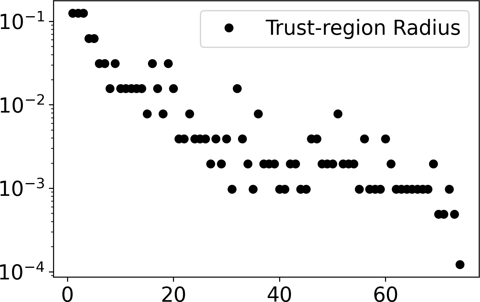
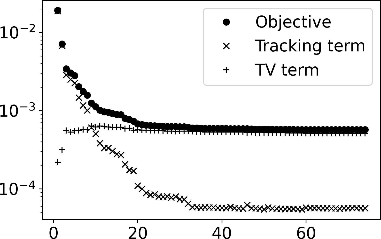
Figure 1: Trust-region radius upon acceptance (left) and objective value (right) achieved over the iterations of Algorithm 1.

Our implementation of Algorithm 1 is able to compute a non-trivial control whose level sets partition the control domain. In particular, the level sets to the values $1$ and $2$ of the final control consist of several disjoint connected components. We illustrate this by plotting the controls and corresponding states for iterations 3, 25, and 73 in Fig. 2.

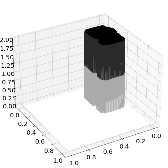
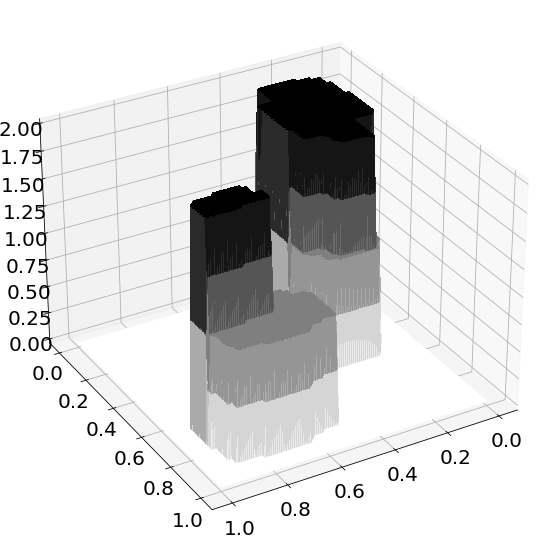
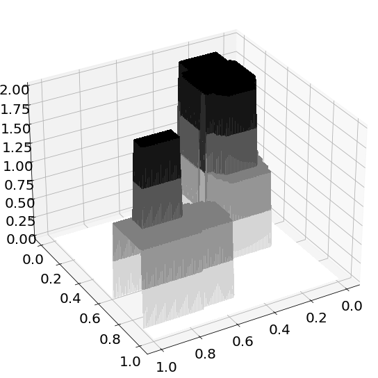
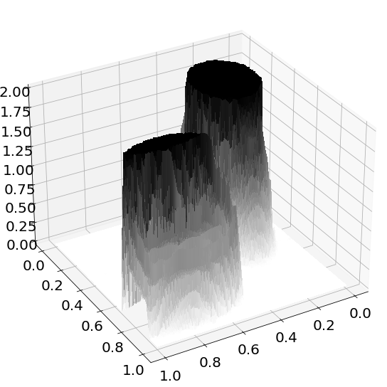
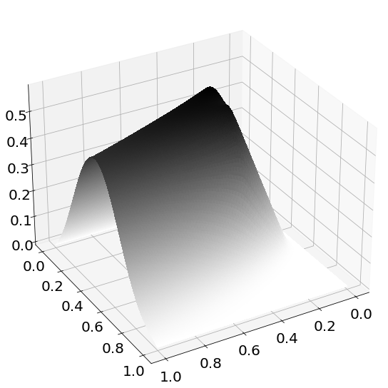
(a) It # 3

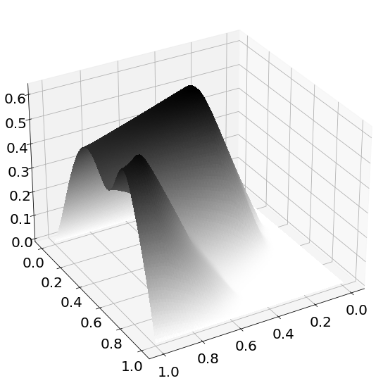
(b) It # 25

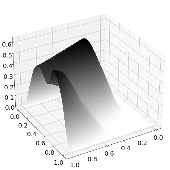
(c) It # 73

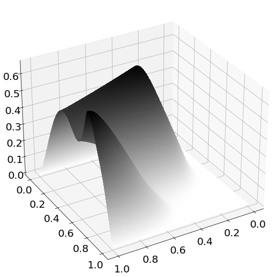
(d) Relaxation

Figure 2: Control iterates (top) and corresponding states (bottom) produced by Algorithm 1 for iterations 3, 25, and 73 as well as for the final iteration of the relaxation.

8 Conclusion

We have investigated TV-regularized integer optimal control problems on multi-dimensional domains. We have derived a first-order optimality condition for locally optimal solutions of Eq. P by means of local variations that yield feasible perturbations of the level sets of our integer-valued control inputs. In order to solve Eq. P, we have analyzed the asymptotics of the trust-region algorithm proposed in [25] for the case $d\geq 2$. We have proved $\Gamma$-convergence of the trust-region subproblems with respect to strict convergence of the linearization point. We have established a sufficient decrease condition based on local variations, which in turn leads to convergence of the iterates of the trust-region algorithm to first-order optimal points.

In order to obtain a useful method in practice, it is important to extend our function space analysis with sophisticated discretizations and a corresponding numerical analysis. Moreover, we have experienced numerical difficulties and very long compute times of the integer programming solver when choosing finer control discretizations for the example in Section 7 so that scaling and stabilization techniques as well as efficient algorithms for solving the discretized trust-region subproblems remain open questions as well.

Appendix A Auxiliary Results

Proof of Lemma 2.1.

Claim (a) follows, e.g., from [25, Lem. 2.2]. Claim (b) follows from [2, Thm.  3.40], which states that for $v\in\operatorname*{BV_{V}}(\Omega)$ the sets

$$F_{i}\coloneqq\left\{x\in\Omega\,\middle|\,v(x)>\nu_{i}-\varepsilon\right\}=\left\{x\in\Omega\,\middle|\,v(x)\geq\nu_{i}\right\}$$

with $\varepsilon\in(0,1)$ and $i\in\{1,\dots,M\}$ are of finite perimeter in $\Omega$. Without loss of generality, we may assume $\nu_{i}>\nu_{i+1}$ for all $i\in\{1,\dots,M-1\}$. We define $E_{1}\coloneqq F_{1}=v^{-1}(\{\nu_{1}\})$ and $E_{i}\coloneqq F_{i}\setminus F_{i-1}=v^{-1}(\{\nu_{i}\})$ for all $i\in\{2,\dots,M\}$. This yields $P(E_{1},\Omega)=P(F_{1},\Omega)<\infty$, $P(E_{i},\Omega)\leq P(F_{i},\Omega)+P(F_{i-1},\Omega)<\infty$ for all $i\in\{2,\dots,M\}$, and $v=\sum_{i=1}^{M}\nu_{i}\chi_{E_{i}}$.

In order to prove (c), let $\sum_{i=1}^{M}\nu_{i}\chi_{E_{i}}=v\in\operatorname*{BV_{V}}(\Omega)$ as in (b). By means of Theorems 3.36 and 3.59 in [2], we obtain

$$Dv=\sum_{i=1}^{M}\nu_{i}D\chi_{E_{i}}=-\sum_{i=1}^{M}\nu_{i}n_{E_{i}}\mathcal{H}^{d-1}\mathbin{\vrule height=6.88889pt,depth=0.0pt,width=0.55974pt\vrule height=0.55974pt,depth=0.0pt,width=5.59721pt}(\partial^{*}E_{i}\cap\Omega),$$ (20)

where the functions $\chi_{E_{i}}$ are considered as elements of $\operatorname*{BV}(\Omega)$. Next, we prove the identity

$$Dv=\sum_{i=1}^{M-1}\sum_{j=i+1}^{M}(\nu_{j}-\nu_{i})n_{E_{i}}\mathcal{H}^{d-1}\mathbin{\vrule height=6.88889pt,depth=0.0pt,width=0.55974pt\vrule height=0.55974pt,depth=0.0pt,width=5.59721pt}(\partial^{*}E_{i}\cap\partial^{*}E_{j}\cap\Omega),$$ (21)

where $Dv$ denotes the Radon measure that is the distributional derivative of $v\in\operatorname*{BV_{V}}(\Omega)$ and $n_{E_{i}}$ denotes the unit outer normal vector of $E_{i}$ that is defined on $\partial^{*}E_{i}$. To this end, we observe that every $x\in\partial^{*}E_{i}\cap\Omega$ is a point of density $\tfrac{1}{2}$ for $E_{i}$ and, consequently, cannot be a point of density $1$ for any $E_{j}$, $j\in\{1,\ldots,M\}$. We apply Theorem 4.17 in [2] to the right hand side of (20) and obtain

$$Dv=-\sum_{i=1}^{M}\nu_{i}n_{E_{i}}\mathcal{H}^{d-1}\mathbin{\vrule height=6.88889pt,depth=0.0pt,width=0.55974pt\vrule height=0.55974pt,depth=0.0pt,width=5.59721pt}\Bigg{(}\underset{j\neq i}{\bigcup_{j=1}^{M}}\underbrace{\partial^{*}E_{i}\cap\partial^{*}E_{j}\cap\Omega}_{\eqqcolon A_{ij}}\Bigg{)},$$

where we have used that $x\in\Omega$ can be a point of density $\tfrac{1}{2}$ for at most two of the disjoint sets $E_{k}$, $k\in\{1,\ldots,M\}$. Using this observation again, we obtain that the sets $A_{ij}$ are pairwise disjoint, which implies

$$Dv=-\sum_{i=1}^{M-1}\sum_{j=i+1}^{M}(\nu_{i}n_{E_{i}}+\nu_{E_{j}}n_{E_{j}})\mathcal{H}^{d-1}\mathbin{\vrule height=6.88889pt,depth=0.0pt,width=0.55974pt\vrule height=0.55974pt,depth=0.0pt,width=5.59721pt}(\partial^{*}E_{i}\cap\partial^{*}E_{j}\cap\Omega).$$ (22)

Then (21) follows because $n_{E_{j}}=-n_{E_{i}}$ on $\partial^{*}E_{i}\cap\partial^{*}E_{j}$. Because every $x\in\partial^{*}E_{i}\cap\partial^{*}E_{j}$ has density $\frac{1}{2}$ with respect to $E_{i}$ and $E_{j}$ and therefore density $1$ with respect to $\Omega$, which yields $x\notin\partial^{*}\Omega$, which is a subset of the points of density $\tfrac{1}{2}$ with respect to $\Omega$. Since $\Omega$ has Lipschitz boundary, there holds $\mathcal{H}^{d-1}(\partial\Omega\setminus\partial^{*}\Omega)=0$, see [2, Prop. 3.62]. In combination, we get

$$\mathcal{H}^{d-1}((\partial^{*}E_{i}\cap\partial^{*}E_{j})\setminus\Omega)=0.$$

Moreover, because the $A_{ij}$ are pairwise disjoint, the measures $\mathcal{H}^{d-1}\mathbin{\vrule height=6.88889pt,depth=0.0pt,width=0.55974pt\vrule height=0.55974pt,depth=0.0pt,width=5.59721pt}A_{ij}$ are pairwise singular. Thus we deduce with $\operatorname*{TV}(v)=|Dv|(\Omega)$ and $\|n_{E_{i}}(x)\|=1$ for (21) that

$$\operatorname*{TV}(v)=\sum_{i=1}^{M-1}\sum_{j=i+1}^{M}|\nu_{i}-\nu_{j}|\mathcal{H}^{d-1}(\partial^{*}E_{i}\cap\partial^{*}E_{j}),$$

which gives (1). Moreover,

$$\begin{aligned} \infty>\operatorname*{TV}(v)&=\sum_{i=1}^{M-1}\sum_{j=i+1}^{M}|\nu_{i}-\nu_{j}|\mathcal{H}^{d-1}(\partial^{*}E_{i}\cap\partial^{*}E_{j})\\ &\geq\frac{1}{2}\sum_{i=1}^{M}\underset{j\neq i}{\sum_{j=1}^{M}}\mathcal{H}^{d-1}(\partial^{*}E_{i}\cap\partial^{*}E_{j})\\ &\geq\frac{1}{2}\sum_{i=1}^{M}\mathcal{H}^{d-1}(\partial^{*}E_{i}\cap\Omega)=\frac{1}{2}\sum_{i=1}^{M}P(E_{i},\Omega),\end{aligned}$$

which gives (2). ∎

Lemma A.1.

Let $g_{i}:\mathbb{R}^{d}\to\mathbb{R}^{d}$, $i\in J$ for a (potentially uncountable) index set $J$ be a family of functions such that for $\delta\in(0,1)$ there exists a set $J_{\delta}\subset J$ such that for all $x\in\mathbb{R}^{d}$ it holds that $\|\nabla g_{i}(x)-I\|\leq\delta$ for all $i\in J_{\delta}$. Then for all $i\in J_{\delta}$ the function $g_{i}$ is a diffeomorphism.

Proof.

The uniform estimate $\|\nabla g_{i}(x)-I\|\leq\delta$ implies that for $\delta<1$ the functions $G_{i}^{y}:\mathbb{R}^{d}\ni x\mapsto y+(x-g_{i}(x))\in\mathbb{R}^{d}$, $i\in J_{\delta}$, have a unique fixed point for all $y\in\mathbb{R}^{d}$ by virtue of the Banach fixed point theorem. In particular, $x=G^{y}_{i}(x)$ if and only if $y=g_{i}(x)$. Thus $g_{i}$ is invertible. Moreover, $\nabla g_{i}(x)$ is invertible for all $x\in\mathbb{R}^{d}$ and thus the inverse function theorem implies that $g_{i}$ is a diffeomorphism. ∎

Lemma A.2.

Let $f_{t}\coloneqq I+t\phi$ for $\phi\in C_{c}^{\infty}(\Omega;\mathbb{R}^{d})$. Then there is $\varepsilon>0$ such that $g_{t}\coloneqq f_{t}^{-1}=I-t\phi\circ g_{t}$ for $t\in(-\varepsilon,\varepsilon)$. Moreover, the mapping $(-\varepsilon,\varepsilon)\ni t\mapsto g_{t}(y)\in\mathbb{R}^{d}$ is Lipschitz continuous for each $y\in\mathbb{R}^{d}$ and $\nabla g_{t}(y)\to I$ as $t\to 0$ uniformly for $y\in\mathbb{R}^{d}$.

Proof.

Let $\phi\in C_{c}^{\infty}(\Omega;\mathbb{R}^{d})$. We denote the Lipschitz constant of $\phi$ by $L_{\phi}$. Let $\varepsilon<\frac{1}{L_{\phi}}$. Define $T_{y}:\mathbb{R}^{d}\to\mathbb{R}^{d}$, $T_{y}\coloneqq y-t\phi$, for fixed $t\in(-\varepsilon,\varepsilon)$ and $y\in\mathbb{R}^{d}$. Then $T_{y}$ is a contraction mapping since for arbitrary $x,z\in\mathbb{R}^{d}$ it holds that

$$\|T_{y}(x)-T_{y}(z)\|=|t|\|\phi(x)-\phi(z)\|\leq|t|L_{\phi}\|x-z\|.$$

By Banach’s fixed point theorem, there exists a unique fixed point $\tilde{x}_{y}\in\mathbb{R}^{d}$ with $T_{y}(\tilde{x}_{y})=\tilde{x}_{y}$. We define $g_{t}(y)\coloneqq\tilde{x}_{y}$ and prove that $g_{t}=f_{t}^{-1}$. It holds that $g_{t}(y)=T_{y}(\tilde{x}_{y})=y-t\phi(\tilde{x}_{y})=y-t\phi(g_{t}(y))$ for $y\in\mathbb{R}^{d}$ and therefore

$$\|g_{t}(f_{t}(y))-y\| =\|t\phi(y)-t\phi(g_{t}(f_{t}(y)))\|\leq|t|L_{\phi}\|g_{t}(f_{t}(y))-y\|.$$

Since $|t|L_{\phi}<1$, it must hold that $\|g_{t}(f_{t}(y))-y\|=0$.

We now prove the Lipschitz continuity of $g_{t}(y)$ in $t\in(-\varepsilon,\varepsilon)$ for fixed $y\in\mathbb{R}^{d}$. For this, let $t,s\in(-\varepsilon,\varepsilon)$. Then

$$\|g_{t}(y)-g_{s}(y)\| =\|s\phi(g_{s}(x))-t\phi(g_{t}(y))\|\leq|s-t|\|\phi(g_{s}(y))\|+|t|L_{\phi}\|g_{s}(y)-g_{t}(y)\|$$

and therefore

$$\|g_{t}(y)-g_{s}(y)\|\leq|t-s|\frac{\|\phi(g_{s}(y))\|}{1-|t|L_{\phi}}<|t-s|\frac{\|\phi(g_{s}(y))\|}{1-\varepsilon L_{\phi}}\leq|t-s|C$$

with $C=(1-\varepsilon L_{\phi})^{-1}\max_{x\in\bar{\Omega}}\|\phi(x)\|<\infty$, only depending on $\phi$ but not on $y$.

In order to prove the convergence of $\nabla g_{t}(y)$, we now choose $\varepsilon$ small enough so that Lemma A.1 gives the existence of $(\nabla f_{t}(x))^{-1}$, which we write as its Neumann series $(\nabla f_{t}(x))^{-1}=I+\sum_{k=1}^{\infty}(-1)^{k}t^{k}\nabla\phi(x)^{k}$. By the inverse function theorem we have

$$\nabla g_{t}(y)=(\nabla f_{t}(g_{t}(y)))^{-1}=I+\sum_{k=1}^{\infty}(-1)^{k}t^{k}\nabla\phi(g_{t}(y))^{k}.$$

Thus, for $|t|$ sufficiently small (that is by potentially further reducing $\varepsilon$)

$$\|I-\nabla g_{t}(y)\| \leq\sum_{k=1}^{\infty}|t|^{k}\|\nabla\phi(g_{t}(y))\|^{k}\leq\sum_{k=1}^{\infty}|t|^{k}M^{k}=\frac{|t|M}{1-|t|M}\to 0$$

as $|t|\to 0$ uniformly for all $y\in\mathbb{R}^{d}$ with $M\coloneqq\max_{x\in\bar{\Omega}}\|\nabla\phi(x)\|<\infty$. ∎

Lemma A.3.

Let $E,F\subset\Omega$ be sets of finite perimeter. Then there holds

$$\partial^{*}(E\cup F)\subset\partial^{e}E\cup\partial^{e}F\text{ and }\partial^{*}(E\setminus F)\subset\partial^{e}E\cup\partial^{e}F.$$

In particular, there holds

$$\mathcal{H}^{d-1}(\partial^{*}(E\cup F))\leq\mathcal{H}^{d-1}(\partial^{*}E\cup\partial^{*}F)\text{ and }\mathcal{H}^{d-1}(\partial^{*}(E\setminus F))\leq\mathcal{H}^{d-1}(\partial^{*}E\cup\partial^{*}F).$$

Proof.

Let $x\in\partial^{*}(E\cup F)$. Then by [2, Thm. 3.61], there holds that $x$ has density $\frac{1}{2}$ regarding $E\cup F$, and therefore

$$\frac{1}{2}=\lim_{r\searrow 0}\frac{\lambda((E\cup F)\cap B_{r}(x)))}{\lambda(B_{r}(x))}\geq\limsup_{r\searrow 0}\frac{\lambda(E\cap B_{r}(x))}{\lambda(B_{r}(x))}$$

and

$$\frac{1}{2}=\lim_{r\searrow 0}\frac{\lambda((E\cup F)\cap B_{r}(x)))}{\lambda(B_{r}(x))}\geq\limsup_{r\searrow 0}\frac{\lambda(F\cap B_{r}(x))}{\lambda(B_{r}(x))}.$$

Moreover,

$$\frac{1}{2}=\lim_{r\searrow 0}\frac{\lambda((E\cup F)\cap B_{r}(x)))}{\lambda(B_{r}(x))}\leq\liminf_{r\searrow 0}\frac{\lambda(E\cap B_{r}(x))}{\lambda(B_{r}(x))}+\frac{\lambda(F\cap B_{r}(x))}{\lambda(B_{r}(x))}$$

and thus

$$\frac{\lambda(E\cap B_{r}(x))}{\lambda(B_{r}(x))}\not\to 0\quad\text{ or }\quad\frac{\lambda(F\cap B_{r}(x))}{\lambda(B_{r}(x))}\not\to 0\quad\text{ as }r\searrow 0.$$

Therefore, $x\in\partial^{e}E\cup\partial^{e}F$. To prove $\partial^{*}(E\setminus F)\subset\partial^{e}E\cup\partial^{e}F$, we use that

$$\mathbb{R}^{d}\setminus(E\setminus F)=(\mathbb{R}^{d}\setminus E)\cup F$$

and obtain

$$\partial^{*}(E\setminus F)=\partial^{*}(\mathbb{R}^{d}\setminus(E\setminus F))=\partial^{*}((\mathbb{R}^{d}\setminus E)\cup F)\subset\partial^{e}(\mathbb{R}^{d}\setminus E)\cup\partial^{e}F=\partial^{e}E\cup\partial^{e}F.$$

The last claim follows from the monotonicity of $\mathcal{H}^{d-1}$ and [2, Thm. 3.61]. ∎

Appendix B Discretized Trust-region Subproblems as Linear Integer Programs

We briefly summarize how the trust-region subproblems yield integer linear programs for a fixed control discretization, see also [25, Section 3.3]. To this end, we fix a partition $\mathcal{P}$ of $\Omega$ into finitely many polytopes of dimension $d$. We denote the set of interior facets by $\mathcal{E}\subset\mathcal{P}\times\mathcal{P}$. The piecewise constant functions on this partition that attain values in $V$ can be written as $v(x)=\sum_{P\in\mathcal{P}}v_{P}\chi_{P}(x)$ for a.a. $x\in\Omega$ with $v_{P}\in V$. Moreover, for $E=(P_{a},P_{b})\in\mathcal{E}$, we write $[v]_{E}=v_{P_{a}}-v_{P_{b}}$. For such functions $v$, $\bar{v}$ and $g\in L^{2}(\Omega)$ we can rewrite the terms in the trust-region subproblems (TR) as:

$$\operatorname*{TV}(v) =\sum_{E\in\mathcal{E}}\int_{E}\left|[v]_{E}\right|\mathop{}\!\mathrm{d}\mathcal{H}^{d-1}=\sum_{E\in\mathcal{E}}\mathcal{H}^{d-1}(E)\left|[v]_{E}\right|,$$

$$(g,v-\bar{v})_{L^{2}(\Omega)} =\sum_{P\in\mathcal{P}}(v_{P}-\bar{v}_{P})\underbrace{\int_{P}g(x)\mathop{}\!\mathrm{d}x}_{\eqqcolon c_{P}},$$

$$\|v-\bar{v}\|_{L^{1}(\Omega)} =\sum_{P\in\mathcal{P}}|v_{P}-\bar{v}_{P}|\lambda(P).$$

By means of auxiliary variables, we can transform the absolute values into linear inequalities, which gives the resulting integer linear program formulation:

$$(\text{TR-as-IP}(\bar{v},g,\Delta))\coloneqq\left\{\begin{aligned} \min_{v_{P},u_{P},w_{E},\tau}\ &\sum_{P\in\mathcal{P}}c_{P}(v_{P}-\bar{v}_{P})+\alpha\tau-\alpha\operatorname*{TV}(\bar{v})\\ \text{~{}~{}s.t.~{}~{}~{}~{}}\ &-u_{P}\leq v_{P}-\bar{v}_{P}\leq u_{P}\text{ for all }P\in\mathcal{P},\\ &{\sum_{P\in\mathcal{P}}}u_{P}\lambda(P)\leq\Delta,\\ &-w_{E}\leq v_{P_{a}}-v_{P_{b}}\leq w_{E}\text{ for all }E=(P_{a},P_{b})\in\mathcal{E},\\ &{\sum_{E\in\mathcal{E}}}w_{E}\mathcal{H}^{d-1}(E)\leq\omega,\\ &v_{P}\in\{\nu_{1},\ldots,\nu_{M}\}\text{ for all }P\in\mathcal{P}.\end{aligned}\right.$$

References

- [1] G. Allaire. Shape Optimization by the Homogenization Method, volume 146 of Applied Mathematical Sciences. Springer Science & Business Media, 2001.
- [2] L. Ambrosio, N. Fusco, and D. Pallara. Functions of bounded variation and free discontinuity problems, volume 254 of Oxford Mathematical Monographs. Clarendon Press Oxford, 2000.
- [3] F. Bestehorn, C. Hansknecht, C. Kirches, and P. Manns. Mixed-integer optimal control problems with switching costs: a shortest path approach. Mathematical Programming, 188(2):621–652, 2021.
- [4] M. Burger, Y. Dong, and M. Hintermüller. Exact relaxation for classes of minimization problems with binary constraints. arXiv preprint arXiv:1210.7507, 2012.
- [5] A. Chambolle, V. Caselles, D. Cremers, M. Novaga, and T. Pock. An introduction to total variation for image analysis. In Theoretical foundations and numerical methods for sparse recovery, pages 263–340. de Gruyter, 2010.
- [6] A. Chambolle and P.-L. Lions. Image recovery via total variation minimization and related problems. Numerische Mathematik, 76(2):167–188, 1997.
- [7] C. Clason and K. Kunisch. Multi-bang control of elliptic systems. In Annales de l’Institut Henri Poincaré (c) Analysé Non Linéaire, volume 31, pages 1109–1130. Elsevier, 2014.
- [8] C. Clason, C. Tameling, and B. Wirth. Vector-valued multibang control of differential equations. SIAM Journal on Control and Optimization, 56(3):2295–2326, 2018.
- [9] A. De Marchi and M. Gerdts. Sparse switching times optimization and a sweeping hessian proximal method. In Operations Research Proceedings 2019, pages 89–95. Springer, 2020.
- [10] D. Dobson and O. Scherzer. Analysis of regularized total variation penalty methods for denoising. Inverse Problems, 12(5):601, 1996.
- [11] S. Engel, B. Vexler, and P. Trautmann. Optimal finite element error estimates for an optimal control problem governed by the wave equation with controls of bounded variation. IMA Journal of Numerical Analysis, 41(4):2639–2667, 2021.
- [12] M. Gerdts. Solving mixed-integer optimal control problems by Branch&Bound: A case study from automobile test-driving with gear shift. Optimal Control Applications and Methods, 26:1–18, 2005.
- [13] S. Göttlich, A. Potschka, and C. Teuber. A partial outer convexification approach to control transmission lines. Computational Optimization and Applications, 72(2):431–456, 2019.
- [14] S. Göttlich, A. Potschka, and U. Ziegler. Partial outer convexification for traffic light optimization in road networks. SIAM Journal on Scientific Computing, 39(1):B53–B75, 2017.
- [15] Gurobi Optimization, LLC. Gurobi Optimizer Reference Manual, 2022.
- [16] D. Hafemeyer and F. Mannel. A path-following inexact newton method for pde-constrained optimal control in bv. Computational Optimization and Applications, pages 1–42, 2022.
- [17] M. Hahn, S. Leyffer, and S. Sager. Binary optimal control by trust-region steepest descent. Mathematical Programming, pages 1–44, 2022.
- [18] F. M. Hante, R. Krug, and M. Schmidt. Time-domain decomposition for mixed-integer optimal control problems. Optimization Online preprint 2021/08/8550, 2021.
- [19] F. M. Hante, G. Leugering, A. Martin, L. Schewe, and M. Schmidt. Challenges in optimal control problems for gas and fluid flow in networks of pipes and canals: From modeling to industrial applications. In Industrial mathematics and complex systems, pages 77–122. Springer, 2017.
- [20] F. M. Hante and S. Sager. Relaxation methods for mixed-integer optimal control of partial differential equations. Computational Optimization and Applications, 55(1):197–225, 2013.
- [21] M. Hintermüller and C. N. Rautenberg. Optimal selection of the regularization function in a weighted total variation model. part i: Modelling and theory. Journal of Mathematical Imaging and Vision, 59(3):498–514, 2017.
- [22] C. Y. Kaya. Optimal control of the double integrator with minimum total variation. Journal of Optimization Theory and Applications, 185:966–981, 2020.
- [23] C. Kirches, P. Manns, and S. Ulbrich. Compactness and convergence rates in the combinatorial integral approximation decomposition. Mathematical Programming, 2020.
- [24] J. Lellmann, D. A. Lorenz, C.-B. Schönlieb, and T. Valkonen. Imaging with Kantorovich–Rubinstein discrepancy. SIAM Journal on Imaging Sciences, 7(4):2833–2859, 2014.
- [25] S. Leyffer and P. Manns. Sequential linear integer programming for integer optimal control with total variation regularization. arXiv preprint arXiv:2106.13453, 2021.
- [26] J. Lindenstrauss. A short proof of Liapounoff’s convexity theorem. Journal of Mathematics and Mechanics, 15(6):971–972, 1966.
- [27] R. Loxton, Q. Lin, V. Rehbock, and K. L. Teo. Control parameterization for optimal control problems with continuous inequality constraints: New convergence results. Numerical Algebra, Control and Optimization, 2(3):571–599, 2012.
- [28] A. A. Lyapunov. On completely additive vector functions. Izv. Akad. Nauk SSSR, 4:465–478, 1940.
- [29] F. Maggi. Sets of Finite Perimeter and Geometric Variational Problems: An Introduction to Geometric Measure Theory. Number 135. Cambridge University Press, 2012.
- [30] P. Manns. Relaxed multibang regularization for the combinatorial integral approximation. SIAM Journal on Control and Optimization, 59(4):2645–2668, 2021.
- [31] P. Manns, M. Hahn, C. Kirches, S. Leyffer, and S. Sager. On structural similarities of combinatorial integral approximation and binary trust-region steepest descent. arXiv preprint,arXiv:2202.07934, 2022.
- [32] P. Manns and C. Kirches. Multidimensional sum-up rounding for elliptic control systems. SIAM Journal on Numerical Analysis, 58(6):3427–3447, 2020.
- [33] J. Marko and G. Wachsmuth. Integer optimal control problems with total variation regularization: Optimality conditions and fast solution of subproblems. arXiv preprint arXiv:2207.05503, 2022.
- [34] A. Martin, M. Möller, and S. Moritz. Mixed integer models for the stationary case of gas network optimization. Mathematical Programming, 105(2):563–582, 2006.
- [35] H. Maurer and N. P. Osmolovskii. Second order sufficient conditions for time-optimal bang-bang control. SIAM Journal on Control and Optimization, 42(6):2239–2263, 2004.
- [36] T. Munson, J. Sarich, S. Wild, S. Benson, and L.C. McInnes. TAO 3.5 Users Manual. Technical report, Argonne National Laboratory, Mathematics and Computer Science Division, 2015. Technical Report ANL/MCS-TM-322.
- [37] E. Newby and M. M. Ali. A trust-region-based derivative free algorithm for mixed integer programming. Computational Optimization and Applications, 60(1):199–229, 2015.
- [38] F. Rathgeber, D.A. Ham, L. Mitchell, Michael Lange, Fabio Luporini, Andrew TT McRae, Gheorghe-Teodor Bercea, Graham R Markall, and Paul HJ Kelly. Firedrake: automating the finite element method by composing abstractions. ACM Transactions on Mathematical Software (TOMS), 43(3):1–27, 2016.
- [39] L. I. Rudin, S. Osher, and E. Fatemi. Nonlinear total variation based noise removal algorithms. Physica D: Nonlinear Phenomena, 60(1-4):259–268, 1992.
- [40] F. Rüffler and F. M. Hante. Optimal switching for hybrid semilinear evolutions. Nonlinear Analysis: Hybrid Systems, 22:215–227, 2016.
- [41] S. Sager, H. G. Bock, and M. Diehl. The Integer Approximation Error in Mixed-Integer Optimal Control. Mathematical Programming, 133(1–2):1–23, 2012.
- [42] S. Sager, M. Jung, and C. Kirches. Combinatorial integral approximation. Mathematical Methods of Operations Research, 73(3):363–380, 2011.
- [43] S. Sager and C. Zeile. On mixed-integer optimal control with constrained total variation of the integer control. Computational Optimization and Applications, 78(2):575–623, 2021.
- [44] M. Severitt and P. Manns. Efficient solution of discrete subproblems arising in integer optimal control with total variation regularization. arXiv preprint arXiv:2206.01642, 2022.
- [45] O. Sigmund and K. Maute. Topology optimization approaches. Structural and Multidisciplinary Optimization, 48(6):1031–1055, 2013.
- [46] B. Stellato, S. Ober-Blöbaum, and P. J. Goulart. Second-order switching time optimization for switched dynamical systems. IEEE Transactions on Automatic Control, 62(10):5407–5414, 2017.
- [47] L. Tartar. Compensated compactness and applications to partial differential equations. In Nonlinear Analysis and Mechanics: Heriot-Watt symposium, volume 4, pages 136–212, 1979.
- [48] C. R. Vogel and M. E. Oman. Iterative methods for total variation denoising. SIAM Journal on Scientific Computing, 17(1):227–238, 1996.
- [49] R. H. Vogt, S. Leyffer, and T. S. Munson. A mixed-integer pde-constrained optimization formulation for electromagnetic cloaking. SIAM Journal on Scientific Computing, 44(1):B29–B50, 2022.