Linear quadratic mean-field game-team analysis: a mixed coalition approach
Jianhui Huang
majhuang@polyu.edu.hk
Zhenghong Qiu
zhenghong.qiu@connect.polyu.hk
Shujun Wang
wangshujun@sdu.edu.cn
Zhen Wu
wuzhen@sdu.edu.cn
Department of Applied Mathematics, The Hong Kong Polytechnic University, Hong Kong
School of Management, Shandong University, Jinan, Shandong 250100, China
School of Mathematics, Shandong University, Jinan, Shandong 250100, China
Appendix
Jianhui Huang
majhuang@polyu.edu.hk
Zhenghong Qiu
zhenghong.qiu@connect.polyu.hk
Shujun Wang
wangshujun@sdu.edu.cn
Zhen Wu
wuzhen@sdu.edu.cn
Department of Applied Mathematics, The Hong Kong Polytechnic University, Hong Kong
School of Management, Shandong University, Jinan, Shandong 250100, China
School of Mathematics, Shandong University, Jinan, Shandong 250100, China
Abstract
Mean-field theory has been extensively explored in decision analysis of large-scale (LS) systems but traditionally in “pure” cooperative or competitive settings. This leads to the so-called mean-field game (MG) or mean-field team (MT). This paper introduces a new class of LS systems with cooperative inner layer and competitive outer layer, so a “mixed” mean-field analysis is proposed for distributed game-team strategy. A novel asymptotic mixed-equilibrium-optima is also proposed and verified.
keywords:
Mean-field game, Mean-field team, Game-team mixed strategy, Mixed-equilibrium-optima
† † thanks: Corresponding author Shujun Wang. This work was supported by the National Key R&D Program of China (No. 2022YFA1006104), RGC P0037987, the National Natural Science Foundation of China (Nos. 12001320, 11831010, 61961160732), the Natural Science Foundation of Shandong Province (No. ZR2019ZD42), the Taishan Scholars Climbing Program of Shandong (No. TSPD20210302), the Taishan Scholars Young Program of Shandong (No. TSQN202211032) and the Young Scholars Program of Shandong University.
1 Introduction
This paper is inspired by (dynamic) decision of large-scale (LS) systems for which the most salient feature, in linear-quadratic (LQ) setting, is existence of sufficiently many negligible agents interacted among their states or objectives via empirical state-average or control-average. Weakly-coupled LS systems have been found broad applications across economics, finance, biology and engineering. Interested readers may refer [10 ] , [12 ] , etc. For LS systems with highly complex interactions, mean-field theory provides an effective scheme to study its decision asymptotically as population size N → ∞ → 𝑁 N\rightarrow\infty
In principle, decisions of LS systems can be classified into non-cooperative game or cooperative team, relying on coalition structure formalized by involved agents in underlying population. Accordingly, mean-field game (MG) or mean-field team (MT) arise naturally when studying LS asymptotically. Along game-line (MG), all agents, { 𝒜 i } i = 1 N superscript subscript subscript 𝒜 𝑖 𝑖 1 𝑁 \{\mathcal{A}_{i}\}_{i=1}^{N} { 𝒥 i } i = 1 N superscript subscript subscript 𝒥 𝑖 𝑖 1 𝑁 \{\mathcal{J}_{i}\}_{i=1}^{N} [2 ] , [3 ] , [5 ] , [6 ] , [8 ] , [9 ] , [10 ] , [12 ] , [14 ] , [15 ] , [21 ] . Parallel to game, MT forms another appealing line along which { 𝒜 i } i = 1 N superscript subscript subscript 𝒜 𝑖 𝑖 1 𝑁 \{\mathcal{A}_{i}\}_{i=1}^{N} 𝒥 s o c ( N ) = ∑ 𝒥 i superscript subscript 𝒥 𝑠 𝑜 𝑐 𝑁 subscript 𝒥 𝑖 \mathcal{J}_{soc}^{(N)}=\sum\mathcal{J}_{i} [11 ] , [16 ] , [17 ] , [22 ] .
All aforementioned (MG, MT) attempts, albeit well explored, have only been built on a “pure” basis whereby all LS agents are purely cooperative or competitive. However, in reality, LS system often displays some “mixed” behaviors in its agents’ organization with combined game and team. To be explained later, pure basis seems over idealized to fit reality, so some expanded analysis on more realistic mixed basis is strongly suggested.
On one hand, from a “practical” viewpoint, various real environments suggest LS to display some “mix” decision patterns. Indeed, mixed LS come often from economics, engineering, or management, etc., when two or more competitive networks co-exist, e.g., duopoly market with distributed franchisees; adversarial networks with operation knots (e.g., [4 ] , [7 ] ). Specifically, a mixed basis is well-posed whenever classical two-person game or general multiple-person-game are framed with decentralized decisions on their distributed sub-units . By this, original two (multiple) persons or entities still play game, while all sub-units within each entity formalize two (multiple) teams. So a “mixed” basis arises with tangled game and team. On the other hand, from a “mathematical” viewpoint: conceptually, any LS decision can be captured by its underlying coalition matrix (to be introduced in Section 2.3 N × N 𝑁 𝑁 N\times N identical and one matrix, respectively (𝐂 1 subscript 𝐂 1 \mathbf{C}_{1} 𝐂 2 subscript 𝐂 2 \mathbf{C}_{2}
Motivated by above discussions, this paper formulates and analyzes a certain type of mixed game-team problem involving two levels of interactions: cooperative inner layer for weakly-coupled agents and competitive outer layer between sub-systems. This yields an adversarial LS networks with complex interactions inside and outside. Accordingly, our main contributions are as follows:
1.
A new Mix game-team is introduced and studied, which offers a more general LS setting including those classical ones on mean-field game and team.
2.
A coalition matrix representation is formulated to characterize competitive and cooperative structure among weakly-coupled decision makers. Specifically, classical MG and MT correspond to two extreme cases of such coalition structures.
3.
A bilateral person-by-person optimality condition and bilateral variation decomposition are proposed for the first time to design distributed strategy. Wellposedness of associated consistency condition (CC) is also discussed under mild conditions.
4.
A new notion of asymptotic mixed-equilibrium-optima is proposed to mixed LS study, and verified to the derived distributed mixed-game-team strategy asymptotically.
The remainder of this paper is organized as follows. Section 2 3 4 5 6
2 Problem formulation
2.1 Preliminary
Throughout this paper, ∏ product \prod ℝ n × m superscript ℝ 𝑛 𝑚 \mathbb{R}^{n\times m} 𝕊 n superscript 𝕊 𝑛 \mathbb{S}^{n} ( n × m ) 𝑛 𝑚 (n\times m) ( n × n ) 𝑛 𝑛 (n\times n) A 𝐴 A A T superscript 𝐴 𝑇 A^{T} A 𝐴 A ∥ ⋅ ∥ \|\cdot\| ⟨ ⋅ , ⋅ ⟩ ⋅ ⋅
\langle\cdot,\cdot\rangle v 𝑣 v S 𝑆 S ‖ v ‖ S 2 := ⟨ S v , v ⟩ = v T S v assign superscript subscript norm 𝑣 𝑆 2 𝑆 𝑣 𝑣
superscript 𝑣 𝑇 𝑆 𝑣 \|v\|_{S}^{2}:=\langle Sv,v\rangle\!=\!v^{T}Sv S > 0 ( ≥ 0 ) 𝑆 annotated 0 absent 0 S>0\ (\geq 0) S 𝑆 S S ≫ 0 much-greater-than 𝑆 0 S\gg 0 S − ε I ≥ 0 𝑆 𝜀 𝐼 0 S-\varepsilon I\geq 0 ε > 0 𝜀 0 \varepsilon>0
Moreover, we suppose that ( Ω , ℱ , ℙ ) Ω ℱ ℙ (\Omega,\mathcal{F},\mathbb{P}) W 𝑊 W ( W 1 , ⋯ , W N ) subscript 𝑊 1 ⋯ subscript 𝑊 𝑁 (W_{1},\cdots,W_{N}) N 𝑁 N { ℱ ( t ) } t ≥ 0 subscript ℱ 𝑡 𝑡 0 \{\mathcal{F}(t)\}_{t\geq 0} W i ( s ) , 0 ≤ s ≤ t , 1 ≤ i ≤ N formulae-sequence subscript 𝑊 𝑖 𝑠 0
𝑠 𝑡 1 𝑖 𝑁 W_{i}(s),0\leq s\leq t,1\leq i\leq N ℙ − limit-from ℙ \mathbb{P}- ℱ ℱ \mathcal{F} 𝔽 := { ℱ ( t ) } t ≥ 0 assign 𝔽 subscript ℱ 𝑡 𝑡 0 \mathbb{F}:=\{\mathcal{F}(t)\}_{t\geq 0} { ℱ i ( t ) } t ≥ 0 subscript subscript ℱ 𝑖 𝑡 𝑡 0 \{\mathcal{F}_{i}(t)\}_{t\geq 0} W i ( s ) , 0 ≤ s ≤ t subscript 𝑊 𝑖 𝑠 0
𝑠 𝑡 W_{i}(s),0\leq s\leq t ℙ − limit-from ℙ \mathbb{P}- ℱ i subscript ℱ 𝑖 \mathcal{F}_{i} 𝔽 i := { ℱ i ( t ) } t ≥ 0 assign subscript 𝔽 𝑖 subscript subscript ℱ 𝑖 𝑡 𝑡 0 \mathbb{F}_{i}:=\{\mathcal{F}_{i}(t)\}_{t\geq 0} 1 ≤ i ≤ N 1 𝑖 𝑁 1\leq i\leq N ℰ ℰ \mathcal{E} 𝕂 𝕂 \mathbb{K} L ∞ ( 0 , T ; ℰ ) = { x : [ 0 , T ] → ℰ | x is bounded and deterministic } , superscript 𝐿 0 𝑇 ℰ conditional-set 𝑥 → 0 𝑇 conditional ℰ 𝑥 is bounded and deterministic L^{\infty}(0,T;\mathcal{E})=\left\{x:[0,T]\rightarrow\mathcal{E}\big{|}\ x\text{ is bounded and}\ \text{deterministic}\right\}, C ( [ 0 , T ] ; ℰ ) = { x : [ 0 , T ] → ℰ | x is continuous } 𝐶 0 𝑇 ℰ
conditional-set 𝑥 → 0 𝑇 conditional ℰ 𝑥 is continuous C([0,T];\mathcal{E})=\left\{x:[0,T]\rightarrow\mathcal{E}\big{|}\ x\text{ is continuous}\right\} L 𝕂 2 ( 0 , T ; ℰ ) = { x : [ 0 , T ] × Ω → ℰ | x is 𝕂 -progressively L_{\mathbb{K}}^{2}(0,T;\mathcal{E})=\left\{x:[0,T]\times\Omega\rightarrow\mathcal{E}\big{|}\ x\text{ is }\mathbb{K}\text{-progressively}\right. measurable, ∥ x ∥ L 2 := ( 𝔼 ∫ 0 T ∥ x ( t ) ∥ 2 d t ) 1 2 < ∞ } . \text{measurable, }\|x\|_{L^{2}}:=\Big{(}\mathbb{E}{\int_{0}^{T}}\|x(t)\|^{2}dt\Big{)}^{\frac{1}{2}}<\infty\Big{\}}.
2.2 Large-scale system with weak-coupling
In this paper, on ( Ω , ℱ , 𝔽 , ℙ ) Ω ℱ 𝔽 ℙ (\Omega,\mathcal{F},\mathbb{F},\mathbb{P}) N 𝑁 N { 𝒜 i } i ∈ ℐ subscript subscript 𝒜 𝑖 𝑖 ℐ \{\mathcal{A}_{i}\}_{i\in\mathcal{I}} ℐ = { 1 , ⋯ , N } ℐ 1 ⋯ 𝑁 \mathcal{I}=\{1,\cdots,N\} 𝒜 := { 𝒜 i } i ∈ ℐ assign 𝒜 subscript subscript 𝒜 𝑖 𝑖 ℐ \mathcal{A}:=\{\mathcal{A}_{i}\}_{i\in\mathcal{I}} i th superscript 𝑖 th i^{\text{th}} 𝒜 i subscript 𝒜 𝑖 \mathcal{A}_{i} [ 0 , T ] 0 𝑇 [0,T]
𝒮 i : : subscript 𝒮 𝑖 absent \displaystyle\mathcal{S}_{i}: d x i ( t ) = ( A i x i ( t ) + B i u i ( t ) + F i x ( N ) ( t ) ) d t 𝑑 subscript 𝑥 𝑖 𝑡 subscript 𝐴 𝑖 subscript 𝑥 𝑖 𝑡 subscript 𝐵 𝑖 subscript 𝑢 𝑖 𝑡 subscript 𝐹 𝑖 superscript 𝑥 𝑁 𝑡 𝑑 𝑡 \displaystyle dx_{i}(t)\!=\!(A_{i}x_{i}(t)\!+\!B_{i}u_{i}(t)\!+\!F_{i}x^{(N)}(t))dt (1)
+ σ i d W i ( t ) , x i ( 0 ) = ξ i , subscript 𝜎 𝑖 𝑑 subscript 𝑊 𝑖 𝑡 subscript 𝑥 𝑖 0
subscript 𝜉 𝑖 \displaystyle\qquad\qquad\!+\!\sigma_{i}dW_{i}(t),\quad x_{i}(0)\!=\!\xi_{i},
and for the sake of notation simplicity, we denote 𝐮 := ( u 1 , ⋯ , u N ) assign 𝐮 subscript 𝑢 1 ⋯ subscript 𝑢 𝑁 \mathbf{u}:=(u_{1},\cdots,u_{N}) 𝐱 := ( x 1 , ⋯ , x N ) assign 𝐱 subscript 𝑥 1 ⋯ subscript 𝑥 𝑁 \mathbf{x}:=(x_{1},\cdots,x_{N}) 𝒮 := { 𝒮 i } i ∈ ℐ assign 𝒮 subscript subscript 𝒮 𝑖 𝑖 ℐ \mathcal{S}:=\{\mathcal{S}_{i}\}_{i\in\mathcal{I}} 𝒜 i subscript 𝒜 𝑖 \mathcal{A}_{i} x ( N ) superscript 𝑥 𝑁 x^{(N)} 𝒜 i subscript 𝒜 𝑖 \mathcal{A}_{i} O ( 1 N ) 𝑂 1 𝑁 O\left(\frac{1}{N}\right) u i subscript 𝑢 𝑖 u_{i}
𝒥 i ( ξ 0 ; 𝐮 ) = 𝒥 i ( ξ 0 ; u i , 𝐮 − i ) subscript 𝒥 𝑖 subscript 𝜉 0 𝐮
subscript 𝒥 𝑖 subscript 𝜉 0 subscript 𝑢 𝑖 subscript 𝐮 𝑖
\displaystyle\mathcal{J}_{i}(\xi_{0};\mathbf{u})\!=\!\mathcal{J}_{i}(\xi_{0};{u}_{i},{\mathbf{u}}_{-i}) (2)
= \displaystyle\!= 1 2 𝔼 { ∫ 0 T [ ‖ x i ( t ) − Γ i x ( N ) ( t ) ‖ Q i 2 + ‖ u i ( t ) ‖ R i 2 ] 𝑑 t } , 1 2 𝔼 superscript subscript 0 𝑇 delimited-[] superscript subscript norm subscript 𝑥 𝑖 𝑡 subscript Γ 𝑖 superscript 𝑥 𝑁 𝑡 subscript 𝑄 𝑖 2 subscript superscript norm subscript 𝑢 𝑖 𝑡 2 subscript 𝑅 𝑖 differential-d 𝑡 \displaystyle\frac{1}{2}\mathbb{E}\Bigg{\{}{\int_{0}^{T}}\Big{[}\|x_{i}(t)\!-\!\Gamma_{i}x^{(N)}(t)\|_{Q_{i}}^{2}\!+\!\|u_{i}(t)\|^{2}_{R_{i}}\Big{]}dt\Bigg{\}},
where 𝐮 − i = ( u 1 , ⋯ , u i − 1 , u i + 1 , ⋯ , u N ) subscript 𝐮 𝑖 subscript 𝑢 1 ⋯ subscript 𝑢 𝑖 1 subscript 𝑢 𝑖 1 ⋯ subscript 𝑢 𝑁 \mathbf{u}_{-i}=(u_{1},\cdots,u_{i-1},u_{i+1},\cdots,u_{N}) 1 2 [2 ] , [10 ] , [22 ] , etc). Henceforward, for notation simplicity, we will drop t 𝑡 t i ∈ ℐ 𝑖 ℐ i\in\mathcal{I} i t h superscript 𝑖 𝑡 ℎ i^{th} 𝒰 i = { u i | u i ∈ L 𝔽 i 2 ( 0 , T ; ℝ m ) } subscript 𝒰 𝑖 conditional-set subscript 𝑢 𝑖 subscript 𝑢 𝑖 superscript subscript 𝐿 subscript 𝔽 𝑖 2 0 𝑇 superscript ℝ 𝑚 \mathcal{U}_{i}=\Big{\{}u_{i}|u_{i}\in L_{\mathbb{F}_{i}}^{2}(0,T;\mathbb{R}^{m})\Big{\}} i t h superscript 𝑖 𝑡 ℎ i^{th} 𝒰 i c = { u i | u i ∈ L 𝔽 2 ( 0 , T ; ℝ m ) } superscript subscript 𝒰 𝑖 𝑐 conditional-set subscript 𝑢 𝑖 subscript 𝑢 𝑖 superscript subscript 𝐿 𝔽 2 0 𝑇 superscript ℝ 𝑚 \mathcal{U}_{i}^{c}=\Big{\{}u_{i}|u_{i}\in L_{\mathbb{F}}^{2}(0,T;\mathbb{R}^{m})\Big{\}}
For LS (1 𝔽 𝔽 \mathbb{F} 𝔽 i subscript 𝔽 𝑖 \mathbb{F}_{i}
{ MG: inf u i ( ⋅ ) ∈ 𝒰 i 𝒥 i ( u i ; u − i ) ; MT: inf u ( ⋅ ) ∈ 𝒰 N 𝒥 s o c ( N ) ( u ) := ∑ i = 1 N 𝒥 i ( u ) , 𝒰 N := ∏ i = 1 N 𝒰 i . \left\{\begin{aligned} &\text{{MG:}}\inf_{u_{i}(\cdot)\in\mathcal{U}_{i}}\mathcal{J}_{i}(u_{i};\textbf{u}_{-i});\\
&\text{{MT:}}\inf_{\textbf{u}(\cdot)\in\mathcal{U}^{N}}\mathcal{J}_{soc}^{(N)}(\textbf{u}):=\sum_{i=1}^{N}\mathcal{J}_{i}(\textbf{u}),\quad\mathcal{U}^{N}:=\prod_{i=1}^{N}\mathcal{U}_{i}.\end{aligned}\right. (3)
MG, MT are both decentralized on L 𝔽 i 2 ( 0 , T ; ℝ m ) superscript subscript 𝐿 subscript 𝔽 𝑖 2 0 𝑇 superscript ℝ 𝑚 L_{\mathbb{F}_{i}}^{2}(0,T;\mathbb{R}^{m}) ∏ i = 1 N L 𝔽 i 2 ( 0 , T ; ℝ m ) superscript subscript product 𝑖 1 𝑁 superscript subscript 𝐿 subscript 𝔽 𝑖 2 0 𝑇 superscript ℝ 𝑚 \prod_{i=1}^{N}L_{\mathbb{F}_{i}}^{2}(0,T;\mathbb{R}^{m}) [1 ] , [18 ] , etc.), still centralized on 𝔽 . 𝔽 \mathbb{F}. team cost 𝒥 s o c ( N ) superscript subscript 𝒥 𝑠 𝑜 𝑐 𝑁 \mathcal{J}_{soc}^{(N)} cooperative team-decision u = ( u 1 , ⋯ , u N ) u subscript 𝑢 1 ⋯ subscript 𝑢 𝑁 \textbf{u}=(u_{1},\cdots,u_{N}) competitive 𝒥 i subscript 𝒥 𝑖 \mathcal{J}_{i} u i subscript 𝑢 𝑖 u_{i} coalition matrix insight.
2.3 A coalition matrix representation
First, we introduce nominal cost vector
𝐉 := ( 𝒥 1 , ⋯ , 𝒥 N ) T assign 𝐉 superscript subscript 𝒥 1 ⋯ subscript 𝒥 𝑁 𝑇 \mathbf{J}:=(\mathcal{J}_{1},\cdots,\mathcal{J}_{N})^{T} { 𝒥 i } i = 1 N . superscript subscript subscript 𝒥 𝑖 𝑖 1 𝑁 \{\mathcal{J}_{i}\}_{i=1}^{N}. 𝒜 i , subscript 𝒜 𝑖 \mathcal{A}_{i}, 𝒥 i subscript 𝒥 𝑖 \mathcal{J}_{i} principal cost, while { 𝒥 k } k ≠ i subscript subscript 𝒥 𝑘 𝑘 𝑖 \{\mathcal{J}_{k}\}_{k\neq i} marginal costs. Next, set effective cost vector 𝐊 := ( 𝒦 1 , ⋯ , 𝒦 N ) T assign 𝐊 superscript subscript 𝒦 1 ⋯ subscript 𝒦 𝑁 𝑇 \mathbf{K}:=(\mathcal{K}_{1},\cdots,\mathcal{K}_{N})^{T} 𝒦 i subscript 𝒦 𝑖 \mathcal{K}_{i} 𝒜 i . subscript 𝒜 𝑖 \mathcal{A}_{i}. 𝒦 i ≠ 𝒥 i . subscript 𝒦 𝑖 subscript 𝒥 𝑖 \mathcal{K}_{i}\neq\mathcal{J}_{i}.
By matrix operation, 𝐊 = 𝐂 ⋅ 𝐉 𝐊 ⋅ 𝐂 𝐉 \mathbf{K}=\mathbf{C}\cdot\mathbf{J} coalition matrix 𝐂 = [ c i , j ] 1 ≤ i , j ≤ N 𝐂 subscript delimited-[] subscript 𝑐 𝑖 𝑗
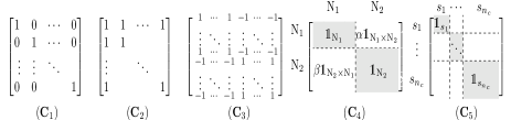
formulae-sequence 1 𝑖 𝑗 𝑁 \mathbf{C}=[c_{i,j}]_{1\leq i,j\leq N} 𝐂 1 subscript 𝐂 1 \mathbf{C}_{1} 𝐂 5 subscript 𝐂 5 \mathbf{C}_{5}
Figure 1: 𝐂 − limit-from 𝐂 \mathbf{C}-
Notably, all coalition 𝐂 − limit-from 𝐂 \mathbf{C}- block feature: the diagonal
“covered” by 1 ≤ n c ≤ N 1 subscript 𝑛 𝑐 𝑁 1\leq n_{c}\leq N one matrix 𝟙 s subscript 1 𝑠 \mathds{1}_{s} 1 1 1 s 1 , ⋯ , s n c subscript 𝑠 1 ⋯ subscript 𝑠 subscript 𝑛 𝑐
s_{1},\cdots,s_{n_{c}} 𝐂 5 subscript 𝐂 5 \mathbf{C}_{5} 𝐂 5 subscript 𝐂 5 \mathbf{C}_{5} 𝐂 4 subscript 𝐂 4 \mathbf{C}_{4} n c = 2 , s 1 = N 1 , s 2 = N 2 = N − N 1 formulae-sequence subscript 𝑛 𝑐 2 formulae-sequence subscript 𝑠 1 subscript 𝑁 1 subscript 𝑠 2 subscript 𝑁 2 𝑁 subscript 𝑁 1 n_{c}=2,\ s_{1}=N_{1},\ s_{2}=N_{2}=N-N_{1} 𝐂 4 subscript 𝐂 4 \mathbf{C}_{4} 𝐂 3 subscript 𝐂 3 \mathbf{C}_{3} α = β = − 1 𝛼 𝛽 1 \alpha=\beta=-1 C 2 subscript C 2 \textbf{C}_{2} α = β = 1 𝛼 𝛽 1 \alpha=\beta=1 ( n c = 1 , s 1 = N ) formulae-sequence subscript 𝑛 𝑐 1 subscript 𝑠 1 𝑁 (n_{c}=1,\ s_{1}=N) 𝐂 5 subscript 𝐂 5 \mathbf{C}_{5} 𝐂 1 subscript 𝐂 1 \mathbf{C}_{1} n c = N , s i ≡ 1 formulae-sequence subscript 𝑛 𝑐 𝑁 subscript 𝑠 𝑖 1 n_{c}=N,\ s_{i}\equiv 1
{ 𝐂 = 𝐂 1 = I N ⟹ ( 𝐊 = 𝐉 ) ⇔ ( 𝒦 i = 𝒥 i ) ⟹ MG ⇔ ( non-cooperative ) { 𝒜 i } i = 1 N ; 𝐂 = 𝐂 2 = 𝟙 N ⟹ ( 𝒦 i ≡ 𝒥 s o c ( N ) = ∑ 𝒥 k ) ⟹ MT ⇔ ( cooperative ) { 𝒜 i } i = 1 N . \left\{\begin{aligned} \mathbf{C}&=\mathbf{C}_{1}=\textbf{I}_{N}\Longrightarrow(\mathbf{K}=\mathbf{J})\Leftrightarrow(\mathcal{K}_{i}=\mathcal{J}_{i})\\
&\Longrightarrow\text{{MG}}\Leftrightarrow(\text{non-cooperative})\ \{\mathcal{A}_{i}\}_{i=1}^{N};\ \\
\mathbf{C}&=\mathbf{C}_{2}=\mathds{1}_{N}\Longrightarrow(\mathcal{K}_{i}\equiv\mathcal{J}^{(N)}_{soc}=\sum\mathcal{J}_{k})\\
&\Longrightarrow\text{{MT}}\Leftrightarrow(\text{cooperative})\ \{\mathcal{A}_{i}\}_{i=1}^{N}.\end{aligned}\right. (4)
So, different 𝐂 − limit-from 𝐂 \mathbf{C}- coalitions among { 𝒜 i } i = 1 N . superscript subscript subscript 𝒜 𝑖 𝑖 1 𝑁 \{\mathcal{A}_{i}\}_{i=1}^{N}. exogenous or endogenous coalition formation (e.g., [13 ] , [20 ] , [23 ] ) as they are economics biased. We observe 𝐂 1 , 𝐂 2 subscript 𝐂 1 subscript 𝐂 2
\mathbf{C}_{1},\mathbf{C}_{2} 𝐂 − limit-from 𝐂 \mathbf{C}- 𝐂 − limit-from 𝐂 \mathbf{C}- 1 < n c < N 1 subscript 𝑛 𝑐 𝑁 1<n_{c}<N 𝐂 3 − 𝐂 5 subscript 𝐂 3 subscript 𝐂 5 \mathbf{C}_{3}\!-\!\mathbf{C}_{5} ℐ 1 = { θ 1 , ⋯ , θ N 1 } subscript ℐ 1 subscript 𝜃 1 ⋯ subscript 𝜃 subscript 𝑁 1 \mathcal{I}_{1}=\{\theta_{1},\cdots,\theta_{N_{1}}\} ℐ 2 = { ϑ 1 , ⋯ , ϑ N 2 } subscript ℐ 2 subscript italic-ϑ 1 ⋯ subscript italic-ϑ subscript 𝑁 2 \mathcal{I}_{2}=\{\vartheta_{1},\cdots,\vartheta_{N_{2}}\} N 1 + N 2 = N subscript 𝑁 1 subscript 𝑁 2 𝑁 N_{1}+N_{2}=N θ i , ϑ j subscript 𝜃 𝑖 subscript italic-ϑ 𝑗
\theta_{i},\ \vartheta_{j} 1 ≤ i ≤ N 1 , 1 ≤ j ≤ N 2 formulae-sequence 1 𝑖 subscript 𝑁 1 1 𝑗 subscript 𝑁 2 1\leq i\leq N_{1},\ 1\leq j\leq N_{2} C 4 : : subscript C 4 absent \textbf{C}_{4}:
𝐂 = 𝐂 4 ⟹ 𝒦 i = 𝐂 subscript 𝐂 4 ⟹ subscript 𝒦 𝑖 absent \displaystyle\mathbf{C}=\mathbf{C}_{4}\Longrightarrow\mathcal{K}_{i}= (5)
{ 𝐉 mix ( 1 ) := 𝒥 soc 1 , ( N ) + α 𝒥 soc 2 , ( N ) , 𝒥 soc 1 , ( N ) := ∑ k ∈ ℐ 1 𝒥 k , 𝐉 mix ( 2 ) := 𝒥 soc 2 , ( N ) + β 𝒥 soc 1 , ( N ) , 𝒥 soc 2 , ( N ) := ∑ k ∈ ℐ 2 𝒥 k , \displaystyle\left\{\begin{aligned} &\mathbf{J}_{\text{mix}}^{(1)}:=\mathcal{J}^{1,(N)}_{\text{soc}}\!+\!\alpha\mathcal{J}^{2,(N)}_{\text{soc}},\quad\mathcal{J}^{1,(N)}_{\text{soc}}:=\sum_{k\in\mathcal{I}_{1}}\mathcal{J}_{k},\\
&\mathbf{J}_{\text{mix}}^{(2)}:=\mathcal{J}^{2,(N)}_{\text{soc}}\!+\!\beta\mathcal{J}^{1,(N)}_{\text{soc}},\quad\mathcal{J}^{2,(N)}_{\text{soc}}:=\sum_{k\in\mathcal{I}_{2}}\mathcal{J}_{k},\end{aligned}\right.
where α , β ∈ ℝ 𝛼 𝛽
ℝ \alpha,\ \beta\in\mathbb{R} k = 1 , 2 𝑘 1 2
k=1,2 π k ( N ) = N k N superscript subscript 𝜋 𝑘 𝑁 subscript 𝑁 𝑘 𝑁 \pi_{k}^{(N)}=\frac{N_{k}}{N} π ( N ) = ( π 1 ( N ) , π 2 ( N ) ) superscript 𝜋 𝑁 superscript subscript 𝜋 1 𝑁 superscript subscript 𝜋 2 𝑁 \pi^{(N)}=(\pi_{1}^{(N)},\pi_{2}^{(N)}) ℐ 1 subscript ℐ 1 \mathcal{I}_{1} ℐ 2 subscript ℐ 2 \mathcal{I}_{2} := { 𝒜 k } k ∈ ℐ 1 assign absent subscript subscript 𝒜 𝑘 𝑘 subscript ℐ 1 :=\{\mathcal{A}_{k}\}_{k\in\mathcal{I}_{1}} := { 𝒜 k } k ∈ ℐ 2 assign absent subscript subscript 𝒜 𝑘 𝑘 subscript ℐ 2 :=\{\mathcal{A}_{k}\}_{k\in\mathcal{I}_{2}} internal MTs. LS1 and LS2 remain competitive outside if α < 0 , β < 0 formulae-sequence 𝛼 0 𝛽 0 \alpha<0,\ \beta<0 α > 0 , β > 0 formulae-sequence 𝛼 0 𝛽 0 \alpha>0,\ \beta>0
2.4 Mixed game-team via coalition
Now, we are ready to formally introduce the “mixed” game-team (Mix ) via coalition matrix representation 𝐂 4 subscript 𝐂 4 \mathbf{C}_{4}
(Mix) { LS1: inf u 1 ( ⋅ ) ∈ 𝐔 ( 1 ) 𝐉 mix ( 1 ) ( u 1 ; u 2 ) , u 1 := ( ⋯ , u k , ⋯ ) | k ∈ ℐ 1 , 𝐔 ( 1 ) := ∏ k ∈ ℐ 1 𝒰 k ; LS2: inf u 2 ( ⋅ ) ∈ 𝐔 ( 2 ) 𝐉 mix ( 2 ) ( u 2 ; u 1 ) , u 2 := ( ⋯ , u k , ⋯ ) | k ∈ ℐ 2 , 𝐔 ( 2 ) := ∏ k ∈ ℐ 2 𝒰 k . \text{{(Mix)}}\left\{\begin{aligned} &\text{{LS1:}}\inf_{\textbf{u}_{1}(\cdot)\in\mathbf{U}^{({1})}}\mathbf{J}_{\text{mix}}^{(1)}(\textbf{u}_{1};\textbf{u}_{2}),\\
&\quad\textbf{u}_{1}:=(\cdots,u_{k},\cdots)|_{k\in\mathcal{I}_{1}},\ \mathbf{U}^{(1)}:=\prod_{k\in\mathcal{I}_{1}}\mathcal{U}_{k};\\
&\text{{LS2:}}\inf_{\textbf{u}_{2}(\cdot)\in\mathbf{U}^{({2})}}\mathbf{J}_{\text{mix}}^{(2)}(\textbf{u}_{2};\textbf{u}_{1}),\\
&\quad\textbf{u}_{2}:=(\cdots,u_{k},\cdots)|_{k\in\mathcal{I}_{2}},\ \mathbf{U}^{(2)}:=\prod_{k\in\mathcal{I}_{2}}\mathcal{U}_{k}.\end{aligned}\right. (6)
To better illustrate the categories of LS1 and LS2 , we need rewrite the dynamics 𝒮 i subscript 𝒮 𝑖 \mathcal{S}_{i} 1
{ d x i ( t ) = ( A 1 x i ( t ) + B 1 u i ( t ) + F 1 x ( N ) ( t ) ) d t + σ 1 ( t ) d W i ( t ) , x i ( 0 ) = ξ i , i ∈ ℐ 1 , d x j ( t ) = ( A 2 x j ( t ) + B 2 u j ( t ) + F 2 x ( N ) ( t ) ) d t + σ 2 ( t ) d W j ( t ) , x j ( 0 ) = η j , j ∈ ℐ 2 , \left\{\begin{aligned} &dx_{i}(t)\!=\!\left(A_{1}x_{i}(t)\!+\!B_{1}u_{i}(t)\!+\!F_{1}x^{(N)}(t)\right)dt\\
&\qquad\qquad\!+\!\sigma_{1}(t)dW_{i}(t),\quad x_{i}(0)\!=\!\xi_{i},\quad i\in\mathcal{I}_{1},\\
&dx_{j}(t)\!=\!\left(A_{2}x_{j}(t)\!+\!B_{2}u_{j}(t)\!+\!F_{2}x^{(N)}(t)\right)dt\\
&\qquad\qquad\!+\!\sigma_{2}(t)dW_{j}(t),\quad x_{j}(0)\!=\!\eta_{j},\quad j\in\mathcal{I}_{2},\end{aligned}\right. (7)
where x ( N ) ( ⋅ ) = 1 N ( ∑ i ∈ ℐ 1 x i ( ⋅ ) + ∑ j ∈ ℐ 2 x j ( ⋅ ) ) superscript 𝑥 𝑁 ⋅ 1 𝑁 subscript 𝑖 subscript ℐ 1 subscript 𝑥 𝑖 ⋅ subscript 𝑗 subscript ℐ 2 subscript 𝑥 𝑗 ⋅ x^{(N)}(\cdot)=\frac{1}{N}\left(\sum_{i\in\mathcal{I}_{1}}x_{i}(\cdot)\!+\!\sum_{j\in\mathcal{I}_{2}}x_{j}(\cdot)\right) 𝐱 1 := ( x θ 1 , ⋯ , x θ N 1 ) assign subscript 𝐱 1 subscript 𝑥 subscript 𝜃 1 ⋯ subscript 𝑥 subscript 𝜃 subscript 𝑁 1 \mathbf{x}_{1}:=(x_{\theta_{1}},\cdots,x_{\theta_{N_{1}}}) 𝐱 2 := ( x ϑ 1 , ⋯ , x ϑ N 2 ) assign subscript 𝐱 2 subscript 𝑥 subscript italic-ϑ 1 ⋯ subscript 𝑥 subscript italic-ϑ subscript 𝑁 2 \mathbf{x}_{2}:=(x_{\vartheta_{1}},\cdots,x_{\vartheta_{N_{2}}}) 2
{ 𝒥 i ( 𝐮 1 ( ⋅ ) , 𝐮 2 ( ⋅ ) ) = 1 2 𝔼 ∫ 0 T [ ‖ x i ( t ) − Γ 1 x ( N ) ( t ) ‖ Q 1 2 + ‖ u i ( t ) ‖ R 1 2 ] 𝑑 t , 𝒥 j ( 𝐮 1 ( ⋅ ) , 𝐮 2 ( ⋅ ) ) = 1 2 𝔼 ∫ 0 T [ ‖ x j ( t ) − Γ 2 x ( N ) ( t ) ‖ Q 2 2 + ‖ u j ( t ) ‖ R 2 2 ] 𝑑 t . \left\{\begin{aligned} &\mathcal{J}_{i}(\mathbf{u}_{1}(\cdot),\mathbf{u}_{2}(\cdot))\\
&=\frac{1}{2}\mathbb{E}\int_{0}^{T}\Big{[}\|x_{i}(t)-\Gamma_{1}x^{(N)}(t)\|_{Q_{1}}^{2}\!+\!\|u_{i}(t)\|^{2}_{R_{1}}\Big{]}dt,\\
&\mathcal{J}_{j}(\mathbf{u}_{1}(\cdot),\mathbf{u}_{2}(\cdot))\\
&=\frac{1}{2}\mathbb{E}\int_{0}^{T}\Big{[}\|x_{j}(t)-\Gamma_{2}x^{(N)}(t)\|_{Q_{2}}^{2}\!+\!\|u_{j}(t)\|^{2}_{R_{2}}\Big{]}dt.\end{aligned}\right. (8)
The agents in { 𝒜 i } i ∈ ℐ 1 subscript subscript 𝒜 𝑖 𝑖 subscript ℐ 1 \{\mathcal{A}_{i}\}_{i\in\mathcal{I}_{1}} { 𝒜 j } j ∈ ℐ 2 subscript subscript 𝒜 𝑗 𝑗 subscript ℐ 2 \{\mathcal{A}_{j}\}_{j\in\mathcal{I}_{2}} 𝐉 mix ( 1 ) superscript subscript 𝐉 mix 1 \mathbf{J}_{\text{mix}}^{(1)} 𝐉 mix ( 2 ) superscript subscript 𝐉 mix 2 \mathbf{J}_{\text{mix}}^{(2)} 5
(H1)
A k , F k , Γ k ∈ ℝ n × n subscript 𝐴 𝑘 subscript 𝐹 𝑘 subscript Γ 𝑘
superscript ℝ 𝑛 𝑛 A_{k},\ F_{k},\ \Gamma_{k}\in\mathbb{R}^{n\times n} B k ∈ ℝ n × m subscript 𝐵 𝑘 superscript ℝ 𝑛 𝑚 B_{k}\in\mathbb{R}^{n\times m} σ k ∈ L ∞ ( 0 , T ; ℝ n ) subscript 𝜎 𝑘 superscript 𝐿 0 𝑇 superscript ℝ 𝑛 \sigma_{k}\in L^{\infty}(0,T;\mathbb{R}^{n}) k = 1 , 2 𝑘 1 2
k=1,2
(H2)
Q k ∈ 𝕊 n subscript 𝑄 𝑘 superscript 𝕊 𝑛 Q_{k}\in\mathbb{S}^{n} R k ∈ 𝕊 m subscript 𝑅 𝑘 superscript 𝕊 𝑚 R_{k}\in\mathbb{S}^{m} Q k > 0 , R k > 0 , formulae-sequence subscript 𝑄 𝑘 0 subscript 𝑅 𝑘 0 Q_{k}>0,\ R_{k}>0, k = 1 , 2 𝑘 1 2
k=1,2
(H3)
{ ξ i } i = 1 N 1 superscript subscript subscript 𝜉 𝑖 𝑖 1 subscript 𝑁 1 \{\xi_{i}\}_{i=1}^{N_{1}} 𝔼 ξ 𝔼 𝜉 \mathbb{E}\xi { η j } j = 1 N 2 superscript subscript subscript 𝜂 𝑗 𝑗 1 subscript 𝑁 2 \{\eta_{j}\}_{j=1}^{N_{2}} 𝔼 η 𝔼 𝜂 \mathbb{E}\eta
(H4)
There exists a probability mass vector π = ( π 1 , π 2 ) 𝜋 subscript 𝜋 1 subscript 𝜋 2 \pi=(\pi_{1},\pi_{2}) lim N → + ∞ π ( N ) = π subscript → 𝑁 superscript 𝜋 𝑁 𝜋 \displaystyle{\lim_{N\rightarrow+\infty}}\pi^{(N)}=\pi min 1 ≤ k ≤ 2 π k > 0 . subscript 1 𝑘 2 subscript 𝜋 𝑘 0 \displaystyle{\min_{1\leq k\leq 2}}\pi_{k}>0.
Thus, we can propose the following homogeneous mixed game-team problem:
Problem 2.1 .
Find a centralized strategy set ( 𝐮 ¯ 1 , 𝐮 ¯ 2 ) subscript ¯ 𝐮 1 subscript ¯ 𝐮 2 \left(\bar{\mathbf{u}}_{1},\bar{\mathbf{u}}_{2}\right) 𝐮 ¯ 1 = ( u ¯ θ 1 , ⋯ , u ¯ θ N 1 ) subscript ¯ 𝐮 1 subscript ¯ 𝑢 subscript 𝜃 1 ⋯ subscript ¯ 𝑢 subscript 𝜃 subscript 𝑁 1 \bar{\mathbf{u}}_{1}\!=\!(\bar{u}_{\theta_{1}},\!\cdots\!,\bar{u}_{\theta_{N_{1}}}) 𝐮 ¯ 2 = ( u ¯ ϑ 1 , ⋯ , u ¯ ϑ N 2 ) subscript ¯ 𝐮 2 subscript ¯ 𝑢 subscript italic-ϑ 1 ⋯ subscript ¯ 𝑢 subscript italic-ϑ subscript 𝑁 2 \bar{\mathbf{u}}_{2}=(\bar{u}_{\vartheta_{1}},\cdots,\bar{u}_{\vartheta_{N_{2}}}) u ¯ i ∈ 𝒰 i subscript ¯ 𝑢 𝑖 subscript 𝒰 𝑖 \bar{u}_{i}\in\mathcal{U}_{i} u ¯ j ∈ 𝒰 j subscript ¯ 𝑢 𝑗 subscript 𝒰 𝑗 \bar{u}_{j}\in\mathcal{U}_{j} i ∈ ℐ 1 𝑖 subscript ℐ 1 i\in\mathcal{I}_{1} j ∈ ℐ 2 𝑗 subscript ℐ 2 j\in\mathcal{I}_{2}
(Mix) { LS1: 𝐉 mix ( 1 ) ( 𝐮 ¯ 1 , 𝐮 ¯ 2 ) = inf 𝐮 1 ∈ 𝐔 ( 1 ) 𝐉 mix ( 1 ) ( 𝐮 1 , 𝐮 ¯ 2 ) , LS2: 𝐉 mix ( 2 ) ( 𝐮 ¯ 1 , 𝐮 ¯ 2 ) = inf 𝐮 2 ∈ 𝐔 ( 2 ) 𝐉 mix ( 2 ) ( 𝐮 ¯ 1 , 𝐮 2 ) . \emph{\text{{(Mix)}}}\left\{\begin{aligned} &\text{\rm{LS1:}}\quad\mathbf{J}_{\text{\rm mix}}^{(1)}(\bar{\mathbf{u}}_{1},\bar{\mathbf{u}}_{2})=\inf_{{\mathbf{u}}_{1}\in\mathbf{U}^{({1})}}\mathbf{J}_{\text{\rm mix}}^{(1)}({\mathbf{u}}_{1},\bar{\mathbf{u}}_{2}),\\
&\text{\rm{LS2:}}\quad\mathbf{J}_{\text{\rm mix}}^{(2)}(\bar{\mathbf{u}}_{1},\bar{\mathbf{u}}_{2})=\inf_{{\mathbf{u}}_{2}\in\mathbf{U}^{({2})}}\mathbf{J}_{\text{\rm mix}}^{(2)}(\bar{\mathbf{u}}_{1},{\mathbf{u}}_{2}).\end{aligned}\right. (9)
(Mix) is meaningful, not only in mathematics as verified by coalition arguments above, but also in practice as supported by real motivations (see [4 ] , [7 ] , etc).
3 Variation synthesis analysis
Initially, we synthesize all response components for 𝐉 mix ( 1 ) superscript subscript 𝐉 mix 1 \mathbf{J}_{\text{mix}}^{(1)} 9 LS1 , LS2 . In what follows, we only focus on the viewpoint of LS1 , and the similar argument can be applied to LS2 .
3.1 Variation decomposition
Let 𝐮 ¯ 1 subscript ¯ 𝐮 1 \bar{\mathbf{u}}_{1} 𝐮 ¯ 2 subscript ¯ 𝐮 2 \bar{\mathbf{u}}_{2} ℐ 1 subscript ℐ 1 \mathcal{I}_{1} ℐ 2 subscript ℐ 2 \mathcal{I}_{2} u i subscript 𝑢 𝑖 u_{i} u ¯ − i = ( u ¯ θ 1 , ⋯ , u ¯ i − 1 , u ¯ i + 1 , ⋯ , u ¯ θ N 1 ) subscript ¯ 𝑢 𝑖 subscript ¯ 𝑢 subscript 𝜃 1 ⋯ subscript ¯ 𝑢 𝑖 1 subscript ¯ 𝑢 𝑖 1 ⋯ subscript ¯ 𝑢 subscript 𝜃 subscript 𝑁 1 \bar{u}_{-i}=(\bar{u}_{\theta_{1}},\cdots,\bar{u}_{i-1},\bar{u}_{i+1},\cdots,\bar{u}_{\theta_{N_{1}}}) 𝐮 ¯ 2 subscript ¯ 𝐮 2 \bar{\mathbf{u}}_{2} k ≠ i 𝑘 𝑖 k\neq i δ u i = u i − u ¯ i 𝛿 subscript 𝑢 𝑖 subscript 𝑢 𝑖 subscript ¯ 𝑢 𝑖 \delta u_{i}=u_{i}-\bar{u}_{i} δ x i = x i − x ¯ i 𝛿 subscript 𝑥 𝑖 subscript 𝑥 𝑖 subscript ¯ 𝑥 𝑖 \delta x_{i}=x_{i}-\bar{x}_{i} δ x k = x k − x ¯ k 𝛿 subscript 𝑥 𝑘 subscript 𝑥 𝑘 subscript ¯ 𝑥 𝑘 \delta x_{k}=x_{k}-\bar{x}_{k} δ x ( N ) = 1 N ∑ k ∈ ℐ 1 ∪ ℐ 2 δ x k 𝛿 superscript 𝑥 𝑁 1 𝑁 subscript 𝑘 subscript ℐ 1 subscript ℐ 2 𝛿 subscript 𝑥 𝑘 \delta x^{(N)}=\frac{1}{N}\sum_{k\in\mathcal{I}_{1}\cup\mathcal{I}_{2}}\delta x_{k} δ 𝒥 soc 1 , ( N ) 𝛿 subscript superscript 𝒥 1 𝑁
soc \delta\mathcal{J}^{1,(N)}_{\text{soc}} δ 𝒥 soc 2 , ( N ) 𝛿 subscript superscript 𝒥 2 𝑁
soc \delta\mathcal{J}^{2,(N)}_{\text{soc}} 𝒥 soc 1 , ( N ) subscript superscript 𝒥 1 𝑁
soc \mathcal{J}^{1,(N)}_{\text{soc}} 𝒥 soc 2 , ( N ) subscript superscript 𝒥 2 𝑁
soc \mathcal{J}^{2,(N)}_{\text{soc}} δ u i 𝛿 subscript 𝑢 𝑖 \delta u_{i}
{ d δ x i ( δ u i ) = [ A 1 δ x i ( δ u i ) + B 1 δ u i + F 1 δ x ( N ) ( δ u i ) ] d t , δ x i ( 0 ) = 0 , d δ x k ( δ u i ) = [ A 1 δ x k ( δ u i ) + F 1 δ x ( N ) ( δ u i ) ] d t , δ x k ( 0 ) = 0 , k ∈ ℐ 1 , k ≠ i , d δ x k ( δ u i ) = [ A 2 δ x k ( δ u i ) + F 2 δ x ( N ) ( δ u i ) ] d t , δ x k ( 0 ) = 0 , k ∈ ℐ 2 . \left\{\begin{aligned} &d\delta x_{i}(\delta u_{i})\!=\!\left[A_{1}\delta x_{i}(\delta u_{i})\!+\!B_{1}\delta u_{i}\!+\!F_{1}\delta x^{(N)}(\delta u_{i})\right]dt,\\
&\quad\ \delta x_{i}(0)\!=\!0,\\
&d\delta x_{k}(\delta u_{i})\!=\!\left[A_{1}\delta x_{k}(\delta u_{i})\!+\!F_{1}\delta x^{(N)}(\delta u_{i})\right]dt,\\
&\quad\ \delta x_{k}(0)\!=\!0,\ k\in\mathcal{I}_{1},\ k\neq i,\\
&d\delta x_{k}(\delta u_{i})\!=\!\left[A_{2}\delta x_{k}(\delta u_{i})\!+\!F_{2}\delta x^{(N)}(\delta u_{i})\right]dt,\\
&\quad\ \delta x_{k}(0)\!=\!0,\ k\in\mathcal{I}_{2}.\\
\end{aligned}\right.
Then we derive the following lemma.
Lemma 3.1 .
δ 𝐉 mix ( 1 ) ( δ u i ) 𝛿 superscript subscript 𝐉 mix 1 𝛿 subscript 𝑢 𝑖 \delta\mathbf{J}_{\text{mix}}^{(1)}(\delta u_{i}) can be represented as
δ 𝐉 mix ( 1 ) ( δ u i ) = 𝔼 ∫ 0 T [ ⟨ Θ ¯ 1 , δ x i ⟩ + ⟨ Θ 2 , δ u i ⟩ + ⟨ Θ ¯ 3 , ∑ k ∈ ℐ 1 , k ≠ i δ x k ⟩ \displaystyle\delta\mathbf{J}_{\text{mix}}^{(1)}(\delta u_{i})=\mathbb{E}\int_{0}^{T}\Big{[}\left\langle\bar{\Theta}_{1},\delta x_{i}\right\rangle\!+\!\left\langle\Theta_{2},\delta u_{i}\right\rangle\!+\!\Big{\langle}\bar{\Theta}_{3},\sum_{k\in\mathcal{I}_{1},k\neq i}\delta x_{k}\Big{\rangle} (10)
+ ⟨ Θ ¯ 4 , ∑ k ∈ ℐ 2 δ x k ⟩ + ∑ k ∈ ℐ 1 , k ≠ i ⟨ Θ 5 k , δ x k ⟩ + ∑ k ∈ ℐ 2 ⟨ Θ 6 k , δ x k ⟩ ] d t + ε i 1 , \displaystyle\ +\Big{\langle}\bar{\Theta}_{4},\sum_{k\in\mathcal{I}_{2}}\delta x_{k}\Big{\rangle}\!+\!\sum_{k\in\mathcal{I}_{1},k\neq i}\left\langle\Theta_{5}^{k},\delta x_{k}\right\rangle\!+\!\sum_{k\in\mathcal{I}_{2}}\left\langle\Theta_{6}^{k},\delta x_{k}\right\rangle\Big{]}dt\!+\!\varepsilon^{i}_{1},
where
ε 1 i = 𝔼 ∫ 0 T [ \displaystyle\varepsilon^{i}_{1}=\mathbb{E}\int_{0}^{T}\Big{[} ⟨ Θ 1 − Θ ¯ 1 , δ x i ⟩ + ⟨ Θ 3 − Θ ¯ 3 , ∑ k ∈ ℐ 1 , k ≠ i δ x k ⟩ subscript Θ 1 subscript ¯ Θ 1 𝛿 subscript 𝑥 𝑖
subscript Θ 3 subscript ¯ Θ 3 subscript formulae-sequence 𝑘 subscript ℐ 1 𝑘 𝑖 𝛿 subscript 𝑥 𝑘
\displaystyle\left\langle\Theta_{1}-\bar{\Theta}_{1},\delta x_{i}\right\rangle\!+\!\Big{\langle}\Theta_{3}-\bar{\Theta}_{3},\sum_{k\in\mathcal{I}_{1},k\neq i}\delta x_{k}\Big{\rangle}
+ ⟨ Θ 4 − Θ ¯ 4 , ∑ k ∈ ℐ 2 δ x k ⟩ ] d t , \displaystyle\!+\!\Big{\langle}{\Theta}_{4}-\bar{\Theta}_{4},\sum_{k\in\mathcal{I}_{2}}\delta x_{k}\Big{\rangle}\Big{]}dt,
{ Θ 1 = Q 1 x ¯ i − ( Q 1 Γ 1 x ¯ ( N ) + Γ 1 T Q 1 π 1 ( N ) ∑ k ∈ ℐ 1 x ¯ k N 1 − π 1 ( N ) Γ 1 T Q 1 Γ 1 x ¯ ( N ) ) − α ( Γ 2 T Q 2 π 2 ( N ) ∑ k ∈ ℐ 2 x ¯ k N 2 − π 2 ( N ) Γ 2 T Q 2 Γ 2 x ¯ ( N ) ) , Θ 3 = − ( Q 1 Γ 1 x ¯ ( N ) + Γ 1 T Q 1 π 1 ( N ) ∑ k ∈ ℐ 1 x ¯ k N 1 − π 1 ( N ) Γ 1 T Q 1 Γ 1 x ¯ ( N ) ) − α ( Γ 2 T Q 2 π 2 ( N ) ∑ k ∈ ℐ 2 x ¯ k N 2 − π 2 ( N ) Γ 2 T Q 2 Γ 2 x ¯ ( N ) ) , Θ 4 = − α ( Q 2 Γ 2 x ¯ ( N ) + Γ 2 T Q 2 π 2 ( N ) ∑ k ∈ ℐ 2 x ¯ k N 2 − π 2 ( N ) Γ 2 T Q 2 Γ 2 x ¯ ( N ) ) − ( Γ 1 T Q 1 π 1 ( N ) ∑ k ∈ ℐ 1 x ¯ k N 1 − π 1 ( N ) Γ 1 T Q 1 Γ 1 x ¯ ( N ) ) , Θ 2 = R 1 , Θ 5 k = Q 1 x ¯ k , Θ 6 k = α Q 2 x ¯ k , Θ ¯ 1 = Q 1 x ¯ i − ( Q 1 Γ 1 𝐦 ¯ + Γ 1 T Q 1 π 1 𝐦 ¯ 1 − π 1 Γ 1 T Q 1 Γ 1 𝐦 ¯ ) − α ( Γ 2 T Q 2 π 2 𝐦 ¯ 2 − π 2 Γ 2 T Q 2 Γ 2 𝐦 ¯ ) , Θ ¯ 3 = − ( Q 1 Γ 1 𝐦 ¯ + Γ 1 T Q 1 π 1 𝐦 ¯ 1 − π 1 Γ 1 T Q 1 Γ 1 𝐦 ¯ ) − α ( Γ 2 T Q 2 π 2 𝐦 ¯ 2 − π 2 Γ 2 T Q 2 Γ 2 𝐦 ¯ ) , \left\{\begin{aligned} &\Theta_{1}=Q_{1}\bar{x}_{i}\!-\!\left(Q_{1}\Gamma_{1}\bar{x}^{(N)}\!+\!\Gamma_{1}^{T}Q_{1}\pi_{1}^{(N)}\frac{\sum_{k\in\mathcal{I}_{1}}\bar{x}_{k}}{N_{1}}\!-\!\pi_{1}^{(N)}\Gamma_{1}^{T}Q_{1}\Gamma_{1}\bar{x}^{(N)}\right)\\
&\qquad\qquad\!-\!\alpha\left(\Gamma_{2}^{T}Q_{2}\pi_{2}^{(N)}\frac{\sum_{k\in\mathcal{I}_{2}}\bar{x}_{k}}{N_{2}}\!-\!\pi_{2}^{(N)}\Gamma_{2}^{T}Q_{2}\Gamma_{2}\bar{x}^{(N)}\right),\\
&\Theta_{3}=-\left(Q_{1}\Gamma_{1}\bar{x}^{(N)}\!+\!\Gamma_{1}^{T}Q_{1}\pi_{1}^{(N)}\frac{\sum_{k\in\mathcal{I}_{1}}\bar{x}_{k}}{N_{1}}\!-\!\pi_{1}^{(N)}\Gamma_{1}^{T}Q_{1}\Gamma_{1}\bar{x}^{(N)}\right)\\
&\qquad\qquad\!-\!\alpha\left(\Gamma_{2}^{T}Q_{2}\pi_{2}^{(N)}\frac{\sum_{k\in\mathcal{I}_{2}}\bar{x}_{k}}{N_{2}}\!-\!\pi_{2}^{(N)}\Gamma_{2}^{T}Q_{2}\Gamma_{2}\bar{x}^{(N)}\right),\\
&\Theta_{4}=-\alpha\left(Q_{2}\Gamma_{2}\bar{x}^{(N)}\!+\!\Gamma_{2}^{T}Q_{2}\pi_{2}^{(N)}\frac{\sum_{k\in\mathcal{I}_{2}}\bar{x}_{k}}{N_{2}}\!-\!\pi_{2}^{(N)}\Gamma_{2}^{T}Q_{2}\Gamma_{2}\bar{x}^{(N)}\right)\\
&\qquad\qquad\!-\!\left(\Gamma_{1}^{T}Q_{1}\pi_{1}^{(N)}\frac{\sum_{k\in\mathcal{I}_{1}}\bar{x}_{k}}{N_{1}}\!-\!\pi_{1}^{(N)}\Gamma_{1}^{T}Q_{1}\Gamma_{1}\bar{x}^{(N)}\right),\\
&\Theta_{2}=R_{1},\quad\Theta_{5}^{k}=Q_{1}\bar{x}_{k},\quad\Theta_{6}^{k}=\alpha Q_{2}\bar{x}_{k},\\
&\bar{\Theta}_{1}=Q_{1}\bar{x}_{i}\!-\!\left(Q_{1}\Gamma_{1}\bar{\mathbf{m}}\!+\!\Gamma_{1}^{T}Q_{1}\pi_{1}\bar{\mathbf{m}}_{1}\!-\!\!\pi_{1}\Gamma_{1}^{T}Q_{1}\Gamma_{1}\bar{\mathbf{m}}\right)\\
&\qquad\qquad\!-\!\alpha\left(\Gamma_{2}^{T}Q_{2}\pi_{2}\bar{\mathbf{m}}_{2}\!-\!\!\pi_{2}\Gamma_{2}^{T}Q_{2}\Gamma_{2}\bar{\mathbf{m}}\right),\\
&\bar{\Theta}_{3}=-\left(Q_{1}\Gamma_{1}\bar{\mathbf{m}}\!+\!\Gamma_{1}^{T}Q_{1}\pi_{1}\bar{\mathbf{m}}_{1}\!-\!\pi_{1}\Gamma_{1}^{T}Q_{1}\Gamma_{1}\bar{\mathbf{m}}\right)\\
&\qquad\qquad\!-\!\alpha\left(\Gamma_{2}^{T}Q_{2}\pi_{2}\bar{\mathbf{m}}_{2}\!-\!\pi_{2}\Gamma_{2}^{T}Q_{2}\Gamma_{2}\bar{\mathbf{m}}\right),\\
\end{aligned}\right.
Θ ¯ 4 = − α ( Q 2 Γ 2 𝐦 ¯ + Γ 2 T Q 2 π 2 𝐦 ¯ 2 − π 2 Γ 2 T Q 2 Γ 2 𝐦 ¯ ) subscript ¯ Θ 4 𝛼 subscript 𝑄 2 subscript Γ 2 ¯ 𝐦 superscript subscript Γ 2 𝑇 subscript 𝑄 2 subscript 𝜋 2 subscript ¯ 𝐦 2 subscript 𝜋 2 superscript subscript Γ 2 𝑇 subscript 𝑄 2 subscript Γ 2 ¯ 𝐦 \displaystyle\bar{\Theta}_{4}=-\alpha\left(Q_{2}\Gamma_{2}\bar{\mathbf{m}}\!+\!\Gamma_{2}^{T}Q_{2}\pi_{2}\bar{\mathbf{m}}_{2}\!-\!\pi_{2}\Gamma_{2}^{T}Q_{2}\Gamma_{2}\bar{\mathbf{m}}\right)
− ( Γ 1 T Q 1 π 1 𝐦 ¯ 1 − π 1 Γ 1 T Q 1 Γ 1 𝐦 ¯ ) . superscript subscript Γ 1 𝑇 subscript 𝑄 1 subscript 𝜋 1 subscript ¯ 𝐦 1 subscript 𝜋 1 superscript subscript Γ 1 𝑇 subscript 𝑄 1 subscript Γ 1 ¯ 𝐦 \displaystyle\qquad\qquad\!-\!\left(\Gamma_{1}^{T}Q_{1}\pi_{1}\bar{\mathbf{m}}_{1}\!-\!\pi_{1}\Gamma_{1}^{T}Q_{1}\Gamma_{1}\bar{\mathbf{m}}\right).
Here, 𝐦 ¯ 1 subscript ¯ 𝐦 1 \bar{\mathbf{m}}_{1} 𝐦 ¯ 2 subscript ¯ 𝐦 2 \bar{\mathbf{m}}_{2} 𝐦 ¯ = π 1 𝐦 ¯ 1 + π 2 𝐦 ¯ 2 ¯ 𝐦 subscript 𝜋 1 subscript ¯ 𝐦 1 subscript 𝜋 2 subscript ¯ 𝐦 2 \bar{\mathbf{m}}=\pi_{1}\bar{\mathbf{m}}_{1}\!+\!\pi_{2}\bar{\mathbf{m}}_{2} 1 N 1 ∑ k ∈ ℐ 1 x ¯ k 1 subscript 𝑁 1 subscript 𝑘 subscript ℐ 1 subscript ¯ 𝑥 𝑘 \frac{1}{N_{1}}\sum_{k\in\mathcal{I}_{1}}\bar{x}_{k} 1 N 2 ∑ k ∈ ℐ 2 x ¯ k 1 subscript 𝑁 2 subscript 𝑘 subscript ℐ 2 subscript ¯ 𝑥 𝑘 \frac{1}{N_{2}}\sum_{k\in\mathcal{I}_{2}}\bar{x}_{k} x ¯ ( N ) superscript ¯ 𝑥 𝑁 \bar{x}^{(N)}
3.2 Bilateral duality
Lemma 3.2 .
δ 𝐉 mix ( 1 ) ( δ u i ) 𝛿 superscript subscript 𝐉 mix 1 𝛿 subscript 𝑢 𝑖 \delta\mathbf{J}_{\text{mix}}^{(1)}(\delta u_{i}) can further be represented as
δ 𝐉 mix ( 1 ) ( δ u i ) = 𝔼 ∫ 0 T [ ⟨ Θ ¯ 1 + π 1 F 1 T 𝔼 p k ( 1 ) ∗ + π 2 F 2 T 𝔼 p k ( 2 ) ∗ \displaystyle\delta\mathbf{J}_{\text{mix}}^{(1)}(\delta u_{i})=\mathbb{E}\int_{0}^{T}\Big{[}\left\langle\bar{\Theta}_{1}\!+\!\pi_{1}F_{1}^{T}\mathbb{E}p_{k}^{(1)*}\!+\!\pi_{2}F_{2}^{T}\mathbb{E}p_{k}^{(2)*}\right. (11)
+ π 1 F 1 T p ( 1 ) ∗ + π 2 F 2 T p ( 2 ) ∗ , δ x i ⟩ + ⟨ Θ 2 , δ u i ⟩ ] d t \displaystyle\qquad\left.\!+\!\pi_{1}F_{1}^{T}p^{(1)*}\!+\!\pi_{2}F_{2}^{T}p^{(2)*},\delta x_{i}\right\rangle+\left\langle\Theta_{2},\delta u_{i}\right\rangle\ \Big{]}dt
+ ε 1 i + ε 2 i + ε 3 i , subscript superscript 𝜀 𝑖 1 subscript superscript 𝜀 𝑖 2 subscript superscript 𝜀 𝑖 3 \displaystyle\qquad\!+\!\varepsilon^{i}_{1}\!+\!\varepsilon^{i}_{2}\!+\!\varepsilon^{i}_{3},
where
ε 2 i = 𝔼 ∫ 0 T [ ⟨ Θ ¯ 3 , ∑ k ∈ ℐ 1 , k ≠ i δ x k − x ( 1 ) , ∗ ∗ ⟩ + ⟨ Θ ¯ 4 , ∑ k ∈ ℐ 2 δ x k − x ( 2 ) , ∗ ∗ ⟩ \displaystyle\varepsilon^{i}_{2}\!=\!\mathbb{E}\int_{0}^{T}\Big{[}\Big{\langle}\bar{\Theta}_{3},\sum_{k\in\mathcal{I}_{1},k\neq i}\delta x_{k}\!-\!x^{(1),**}\Big{\rangle}+\Big{\langle}\bar{\Theta}_{4},\sum_{k\in\mathcal{I}_{2}}\delta x_{k}\!-\!x^{(2),**}\Big{\rangle}
+ 1 N 1 ∑ k ∈ ℐ 1 , k ≠ i ⟨ Θ 5 k , N 1 δ x k − x k ( 1 ) , ∗ ⟩ 1 subscript 𝑁 1 subscript formulae-sequence 𝑘 subscript ℐ 1 𝑘 𝑖 superscript subscript Θ 5 𝑘 subscript 𝑁 1 𝛿 subscript 𝑥 𝑘 subscript superscript 𝑥 1
𝑘
\displaystyle\qquad\!+\!\frac{1}{N_{1}}\sum_{k\in\mathcal{I}_{1},k\neq i}\left\langle\Theta_{5}^{k},N_{1}\delta x_{k}\!-\!x^{(1),*}_{k}\right\rangle
+ 1 N 2 ∑ k ∈ ℐ 2 ⟨ Θ 6 k , N 2 δ x k − x k ( 2 ) , ∗ ⟩ ] d t , \displaystyle\qquad+\frac{1}{N_{2}}\sum_{k\in\mathcal{I}_{2}}\left\langle\Theta_{6}^{k},N_{2}\delta x_{k}\!-\!x^{(2),*}_{k}\right\rangle\Big{]}dt,
ε 3 i = 𝔼 ∫ 0 T ⟨ π 1 F 1 T ( ∑ k ∈ ℐ 1 , k ≠ i p k ( 1 ) N 1 − 𝔼 p k ( 1 ) ∗ ) \displaystyle\varepsilon^{i}_{3}\!=\!\mathbb{E}\int_{0}^{T}\Big{\langle}\pi_{1}F_{1}^{T}\Big{(}\frac{\sum_{k\in\mathcal{I}_{1},k\neq i}p_{k}^{(1)}}{N_{1}}\!-\!\mathbb{E}p_{k}^{(1)*}\Big{)}
+ π 2 F 2 T ( ∑ k ∈ ℐ 2 p k ( 2 ) N 2 − 𝔼 p k ( 2 ) ∗ ) + π 1 F 1 T ( p ( 1 ) − p ( 1 ) ∗ ) subscript 𝜋 2 superscript subscript 𝐹 2 𝑇 subscript 𝑘 subscript ℐ 2 superscript subscript 𝑝 𝑘 2 subscript 𝑁 2 𝔼 superscript subscript 𝑝 𝑘 2
subscript 𝜋 1 superscript subscript 𝐹 1 𝑇 superscript 𝑝 1 superscript 𝑝 1
\displaystyle\qquad\!+\!\pi_{2}F_{2}^{T}\Big{(}\frac{\sum_{k\in\mathcal{I}_{2}}p_{k}^{(2)}}{N_{2}}\!-\!\mathbb{E}p_{k}^{(2)*}\Big{)}\!+\!\pi_{1}F_{1}^{T}\left(p^{(1)}\!-\!p^{(1)*}\right)
+ π 2 F 2 T ( p ( 2 ) − p ( 2 ) ∗ ) , δ x i ⟩ d t , \displaystyle\qquad\!+\!\pi_{2}F_{2}^{T}\left(p^{(2)}\!-\!p^{(2)*}\right),\delta x_{i}\Big{\rangle}dt,
and
{ d x k ( 1 ) , ∗ = [ A 1 x k ( 1 ) , ∗ + π 1 F 1 ( δ x i + x ( 1 ) , ∗ ∗ + x ( 2 ) , ∗ ∗ ) ] d t , d x k ( 2 ) , ∗ = [ A 2 x k ( 2 ) , ∗ + π 2 F 2 ( δ x i + x ( 1 ) , ∗ ∗ + x ( 2 ) , ∗ ∗ ) ] d t , d x ( 1 ) , ∗ ∗ = [ A 1 x ( 1 ) , ∗ ∗ + π 1 F 1 ( x ( 1 ) , ∗ ∗ + x ( 2 ) , ∗ ∗ + δ x i ) ] d t , d x ( 2 ) , ∗ ∗ = [ A 2 x ( 2 ) , ∗ ∗ + π 2 F 2 ( x ( 1 ) , ∗ ∗ + x ( 2 ) , ∗ ∗ + δ x i ) ] d t , x k ( 1 ) , ∗ ( 0 ) = 0 , x k ( 2 ) , ∗ ( 0 ) = 0 , x ( 1 ) , ∗ ∗ ( 0 ) = 0 , x ( 2 ) , ∗ ∗ ( 0 ) = 0 , \left\{\begin{aligned} &dx^{(1),*}_{k}\!=\!\Big{[}A_{1}x^{(1),*}_{k}\!+\!\pi_{1}F_{1}(\delta x_{i}\!+\!x^{(1),**}\!+\!x^{(2),**})\Big{]}dt,\\
&dx^{(2),*}_{k}\!=\!\Big{[}A_{2}x^{(2),*}_{k}\!+\!\pi_{2}F_{2}(\delta x_{i}\!+\!x^{(1),**}\!+\!x^{(2),**})\Big{]}dt,\\
&dx^{(1),**}\!=\!\Big{[}A_{1}x^{(1),**}\!+\!\pi_{1}F_{1}(x^{(1),**}\!+\!x^{(2),**}\!+\!\delta x_{i})\Big{]}dt,\\
&dx^{(2),**}\!=\!\Big{[}A_{2}x^{(2),**}\!+\!\pi_{2}F_{2}(x^{(1),**}\!+\!x^{(2),**}\!+\!\delta x_{i})\Big{]}dt,\\
&x^{(1),*}_{k}(0)=0,\ \ x^{(2),*}_{k}(0)=0,\ x^{(1),**}(0)=0,\ x^{(2),**}(0)\!=\!0,\end{aligned}\right.
{ d p k ( 1 ) = − ( Θ 5 k + A 1 T p k ( 1 ) ) d t + q k ( 1 ) d W k + ∑ k ′ ≠ k q k k ′ ( 1 ) d W k ′ , d p k ( 2 ) = − ( Θ 6 k + A 2 T p k ( 2 ) ) d t + q k ( 2 ) d W k + ∑ k ′ ≠ k q k k ′ ( 2 ) d W k ′ , d p ( 1 ) = − ( Θ ¯ 3 + π 1 ∑ k ∈ ℐ 1 , k ≠ i F 1 T p k ( 1 ) N 1 + π 2 ∑ k ∈ ℐ 2 F 2 T p k ( 2 ) N 2 + A 1 T p ( 1 ) + π 1 F 1 T p ( 1 ) + π 2 F 2 T p ( 2 ) ) d t + ∑ q k ′ ( 1 ) d W k ′ , d p ( 2 ) = − ( Θ ¯ 4 + π 1 ∑ k ∈ ℐ 1 , k ≠ i F 1 T p k ( 1 ) N 1 + π 2 ∑ k ∈ ℐ 2 F 2 T p k ( 2 ) N 2 + π 1 F 1 T p ( 1 ) + π 2 F 2 T p ( 2 ) + A 2 T p ( 2 ) ) d t + ∑ q k ′ ( 2 ) d W k ′ , p k ( 1 ) ( T ) = 0 , p k ( 2 ) ( T ) = 0 , p ( 1 ) ( T ) = 0 , p ( 2 ) ( T ) = 0 , \left\{\begin{aligned} &dp_{k}^{(1)}=-\left(\Theta_{5}^{k}\!+\!A_{1}^{T}p_{k}^{(1)}\right)dt\!+\!q_{k}^{(1)}dW_{k}\!+\!{\sum_{k^{\prime}\neq k}}q_{kk^{\prime}}^{(1)}dW_{k^{\prime}},\\
&dp_{k}^{(2)}=-\left(\Theta_{6}^{k}\!+\!A_{2}^{T}p_{k}^{(2)}\right)dt\!+\!{q}_{k}^{(2)}dW_{k}\!+\!{\sum_{k^{\prime}\neq k}}q_{kk^{\prime}}^{(2)}dW_{k^{\prime}},\\
&dp^{(1)}=-\Big{(}\bar{\Theta}_{3}\!+\!\pi_{1}{\frac{\sum_{k\in\mathcal{I}_{1},k\neq i}F_{1}^{T}p_{k}^{(1)}}{N_{1}}}\!+\!\pi_{2}{\frac{\sum_{k\in\mathcal{I}_{2}}F_{2}^{T}p_{k}^{(2)}}{N_{2}}}\\
&\hskip 51.21504pt\!+\!A_{1}^{T}p^{(1)}\!+\!\pi_{1}F_{1}^{T}p^{(1)}\!+\!\pi_{2}F_{2}^{T}p^{(2)}\Big{)}dt\!+\!{\sum}q_{k^{\prime}}^{(1)}dW_{k^{\prime}},\\
&d{p}^{(2)}=-\Big{(}\bar{\Theta}_{4}\!+\!\pi_{1}{\frac{\sum_{k\in\mathcal{I}_{1},k\neq i}F_{1}^{T}p_{k}^{(1)}}{N_{1}}}\!+\!\pi_{2}{\frac{\sum_{k\in\mathcal{I}_{2}}F_{2}^{T}p_{k}^{(2)}}{N_{2}}}\\
&\hskip 51.21504pt\!+\!\pi_{1}F_{1}^{T}p^{(1)}\!+\!\pi_{2}F_{2}^{T}p^{(2)}\!+\!A_{2}^{T}p^{(2)}\Big{)}dt\!+\!{\sum}q_{k^{\prime}}^{(2)}dW_{k^{\prime}},\\
&p_{k}^{(1)}(T)=0,\ p_{k}^{(2)}(T)=0,\ p^{(1)}(T)=0,\ {p}^{(2)}(T)=0,\end{aligned}\right.
{ 𝒫 ^ k ( 2 ) ∗ : d p k ( 1 ) ∗ = − ( Θ 5 k + A 1 T p k ( 1 ) ∗ ) d t + q k ( 1 ) ∗ d W k , 𝒫 ^ k ( 1 ) ∗ : d p k ( 2 ) ∗ = − ( Θ 6 k + A 2 T p k ( 2 ) ∗ ) d t + q k ( 2 ) ∗ d W k , 𝒫 ^ ( 2 ) ∗ : d p ( 1 ) ∗ = − [ Θ ¯ 3 + π 1 F 1 T 𝔼 p k ( 1 ) ∗ + π 2 F 2 T 𝔼 p k ( 2 ) ∗ + ( A 1 T + π 1 F 1 T ) p ( 1 ) ∗ + π 2 F 2 T p ( 2 ) ∗ ] d t , 𝒫 ^ ( 1 ) ∗ : d p ( 2 ) ∗ = − [ Θ ¯ 4 + π 1 F 1 T 𝔼 p k ( 1 ) ∗ + π 2 F 2 T 𝔼 p k ( 2 ) ∗ + π 1 F 1 T p ( 1 ) ∗ + ( π 2 F 2 T + A 2 T ) p ( 2 ) ∗ ] d t , p k ( 1 ) ∗ ( T ) = 0 , p k ( 2 ) ∗ ( T ) = 0 , p ( 1 ) ∗ ( T ) = 0 , p ( 2 ) ∗ ( T ) = 0 . \left\{\begin{aligned} &\widehat{\mathcal{P}}^{(2)*}_{k}:dp_{k}^{(1)*}=-\left(\Theta_{5}^{k}\!+\!A_{1}^{T}p_{k}^{(1)*}\right)dt\!+\!q_{k}^{(1)*}dW_{k},\\
&\widehat{\mathcal{P}}^{(1)*}_{k}:dp_{k}^{(2)*}=-\left(\Theta_{6}^{k}\!+\!A_{2}^{T}p_{k}^{(2)*}\right)dt\!+\!q_{k}^{(2)*}dW_{k},\\
&\widehat{\mathcal{P}}^{(2)*}:dp^{(1)*}\!=\!-\left[\bar{\Theta}_{3}\!+\!\pi_{1}F_{1}^{T}\mathbb{E}p_{k}^{(1)*}\!+\!\pi_{2}F_{2}^{T}\mathbb{E}p_{k}^{(2)*}\right.\\
&\qquad\qquad\left.\!+\!\left(A_{1}^{T}\!+\!\pi_{1}F_{1}^{T}\right)p^{(1)*}\!+\!\pi_{2}F_{2}^{T}p^{(2)*}\right]dt,\\
&\widehat{\mathcal{P}}^{(1)*}:d{p}^{(2)*}=-\left[\bar{\Theta}_{4}\!+\!\pi_{1}F_{1}^{T}\mathbb{E}p_{k}^{(1)*}\!+\!\pi_{2}F_{2}^{T}\mathbb{E}p_{k}^{(2)*}\right.\\
&\qquad\qquad\left.\!+\!\pi_{1}F_{1}^{T}p^{(1)*}\!+\!\left(\pi_{2}F_{2}^{T}\!+\!A_{2}^{T}\right)p^{(2)*}\right]dt,\\
&p_{k}^{(1)*}(T)=0,\ p_{k}^{(2)*}(T)=0,\ p^{(1)*}(T)=0,\ {p}^{(2)*}(T)=0.\end{aligned}\right.\\
An asymptotic “Fréchet response” holds for δ J i ( 1 ) = lim δ 𝐉 mix ( 1 ) ( δ u i ) 𝛿 superscript subscript 𝐽 𝑖 1 𝛿 superscript subscript 𝐉 mix 1 𝛿 subscript 𝑢 𝑖 \delta J_{i}^{(1)}=\lim\delta\mathbf{J}_{\text{mix}}^{(1)}(\delta u_{i})
LS1 : δ J i ( 1 ) = ⟨ Θ † ( x ¯ i , m , P ∗ ) , δ x i ⟩ + ⟨ Θ † † ( u ¯ i ) , δ u i ⟩ LS1 : 𝛿 superscript subscript 𝐽 𝑖 1
superscript Θ † subscript ¯ 𝑥 𝑖 m superscript P 𝛿 subscript 𝑥 𝑖
superscript Θ † absent † subscript ¯ 𝑢 𝑖 𝛿 subscript 𝑢 𝑖
\displaystyle\text{{LS1}:}\ \ \delta J_{i}^{(1)}\!=\!\langle{\Theta}^{{\dagger}}(\bar{x}_{i},\textbf{m},\textbf{P}^{*}),\delta x_{i}\rangle\!+\!\langle\Theta^{{\dagger}{\dagger}}(\bar{u}_{i}),\delta u_{i}\rangle (12)
with Θ † † = R 1 u ¯ i superscript Θ † absent † subscript 𝑅 1 subscript ¯ 𝑢 𝑖 \Theta^{{\dagger}{\dagger}}=R_{1}\bar{u}_{i} Θ † superscript Θ † \Theta^{{\dagger}} ( Θ ¯ 1 , Θ ¯ 3 , Θ ¯ 4 , Θ 5 k , Θ 6 k ) subscript ¯ Θ 1 subscript ¯ Θ 3 subscript ¯ Θ 4 superscript subscript Θ 5 𝑘 superscript subscript Θ 6 𝑘 \left(\bar{\Theta}_{1},\bar{\Theta}_{3},\bar{\Theta}_{4},{\Theta}_{5}^{k},{\Theta}_{6}^{k}\right) m := ( 𝐦 ¯ , 𝐦 ¯ 1 , 𝐦 ¯ 2 ) assign m ¯ 𝐦 subscript ¯ 𝐦 1 subscript ¯ 𝐦 2 \textbf{m}:=(\bar{\mathbf{m}},\bar{\mathbf{m}}_{1},\bar{\mathbf{m}}_{2}) P ^ ∗ := ( 𝒫 ^ k ( 1 ) ∗ , 𝒫 ^ ( 1 ) ∗ ; 𝒫 ^ k ( 2 ) ∗ , 𝒫 ^ ( 2 ) ∗ ) assign superscript ^ P superscript subscript ^ 𝒫 𝑘 1
superscript ^ 𝒫 1
superscript subscript ^ 𝒫 𝑘 2
superscript ^ 𝒫 2
\widehat{\textbf{P}}^{*}:=(\widehat{\mathcal{P}}_{k}^{(1)*},\widehat{\mathcal{P}}^{(1)*};\widehat{\mathcal{P}}_{k}^{(2)*},\widehat{\mathcal{P}}^{(2)*})
4 Distributed design
4.1 Auxiliary control
Motivated by (11 i ∈ ℐ 1 𝑖 subscript ℐ 1 i\in\mathcal{I}_{1}
Problem 4.1 .
Minimize J i ( u i ) subscript 𝐽 𝑖 subscript 𝑢 𝑖 J_{i}(u_{i}) u i ∈ 𝒰 i subscript 𝑢 𝑖 subscript 𝒰 𝑖 u_{i}\in\mathcal{U}_{i}
{ d x i = ( A 1 x i + B 1 u i + F 1 𝐦 ¯ ) d t + σ 1 d W i , x i ( 0 ) = ξ i , i ∈ ℐ 1 , J i ( 1 ) ( u i ) = 1 2 𝔼 ∫ 0 T [ ⟨ Q 1 x i , x i ⟩ + 2 ⟨ S 1 , x i ⟩ + ⟨ R 1 u i , u i ⟩ ] 𝑑 t , S 1 = − ( Q 1 Γ 1 𝐦 ¯ + Γ 1 T Q 1 π 1 𝐦 ¯ 1 − π 1 Γ 1 T Q 1 Γ 1 𝐦 ¯ ) − α ( Γ 2 T Q 2 π 2 𝐦 ¯ 2 − π 2 Γ 2 T Q 2 Γ 2 𝐦 ¯ ) + π 1 F 1 T 𝔼 p k ( 1 ) ∗ + π 2 F 2 T 𝔼 p k ( 2 ) ∗ + π 1 F 1 T p ( 1 ) ∗ + π 2 F 2 T p ( 2 ) ∗ . \left\{\begin{aligned} &dx_{i}\!=\!(A_{1}x_{i}\!+\!B_{1}u_{i}\!+\!F_{1}\bar{\mathbf{m}})dt\!+\!\sigma_{1}dW_{i},\ x_{i}(0)\!=\!\xi_{i},\ i\in\mathcal{I}_{1},\\
&J_{i}^{(1)}(u_{i})\!=\!\frac{1}{2}\mathbb{E}\int_{0}^{T}[\langle Q_{1}x_{i},x_{i}\rangle\!+\!2\langle S_{1},x_{i}\rangle\!+\!\langle R_{1}u_{i},u_{i}\rangle]dt,\\
&S_{1}=\!-\!\left(Q_{1}\Gamma_{1}\bar{\mathbf{m}}\!+\!\Gamma_{1}^{T}Q_{1}\pi_{1}\bar{\mathbf{m}}_{1}\!-\!\pi_{1}\Gamma_{1}^{T}Q_{1}\Gamma_{1}\bar{\mathbf{m}}\right)\\
&\hskip 28.45274pt\!-\!\alpha\left(\Gamma_{2}^{T}Q_{2}\pi_{2}\bar{\mathbf{m}}_{2}\!-\!\pi_{2}\Gamma_{2}^{T}Q_{2}\Gamma_{2}\bar{\mathbf{m}}\right)+\pi_{1}F_{1}^{T}\mathbb{E}p_{k}^{(1)*}\\
&\hskip 28.45274pt\!+\!\pi_{2}F_{2}^{T}\mathbb{E}p_{k}^{(2)*}\!+\!\pi_{1}F_{1}^{T}p^{(1)*}\!+\!\pi_{2}F_{2}^{T}p^{(2)*}.\end{aligned}\right.
The mean-field terms 𝐦 ¯ ¯ 𝐦 \bar{\mathbf{m}} 𝐦 ¯ 1 subscript ¯ 𝐦 1 \bar{\mathbf{m}}_{1} 𝐦 ¯ 2 subscript ¯ 𝐦 2 \bar{\mathbf{m}}_{2} p k ( 1 ) ∗ superscript subscript 𝑝 𝑘 1
p_{k}^{(1)*} p k ( 2 ) ∗ superscript subscript 𝑝 𝑘 2
p_{k}^{(2)*} j ∈ ℐ 2 𝑗 subscript ℐ 2 j\in\mathcal{I}_{2} 3
Problem 4.2 .
Minimize J j ( u j ) subscript 𝐽 𝑗 subscript 𝑢 𝑗 J_{j}(u_{j}) u j ∈ 𝒰 j subscript 𝑢 𝑗 subscript 𝒰 𝑗 u_{j}\in\mathcal{U}_{j}
{ d x j = ( A 2 x j + B 2 u j + F 2 𝐦 ¯ ) d t + σ 2 d W j , x j ( 0 ) = η j , j ∈ ℐ 2 , J j ( 2 ) ( u j ) = 1 2 𝔼 ∫ 0 T [ ⟨ Q 2 x j , x j ⟩ + 2 ⟨ S 2 , x j ⟩ + ⟨ R 2 u j , u j ⟩ ] 𝑑 t , S 2 = − ( Q 2 Γ 2 𝐦 ¯ + Γ 2 T Q 2 π 2 𝐦 ¯ 2 − π 2 Γ 2 T Q 2 Γ 2 𝐦 ¯ ) − α ( Γ 1 T Q 1 π 1 𝐦 ¯ 1 − π 1 Γ 1 T Q 1 Γ 1 𝐦 ¯ ) + π 2 F 2 T 𝔼 p ^ k ( 2 ) ∗ + π 1 F 1 T 𝔼 p ^ k ( 1 ) ∗ + π 2 F 2 T p ^ ( 2 ) ∗ + π 1 F 1 T p ^ ( 1 ) ∗ , \left\{\begin{aligned} &dx_{j}\!=\!(A_{2}x_{j}\!+\!B_{2}u_{j}\!+\!F_{2}\bar{\mathbf{m}})dt\!+\!\sigma_{2}dW_{j},\ x_{j}(0)\!=\!\eta_{j},\ j\in\mathcal{I}_{2},\\
&J_{j}^{(2)}(u_{j})\!=\!\frac{1}{2}\mathbb{E}\int_{0}^{T}[\langle Q_{2}x_{j},x_{j}\rangle\!+\!2\langle S_{2},x_{j}\rangle\!+\!\langle R_{2}u_{j},u_{j}\rangle]dt,\\
&S_{2}=\!-\!\left(Q_{2}\Gamma_{2}\bar{\mathbf{m}}\!+\!\Gamma_{2}^{T}Q_{2}\pi_{2}\bar{\mathbf{m}}_{2}\!-\!\pi_{2}\Gamma_{2}^{T}Q_{2}\Gamma_{2}\bar{\mathbf{m}}\right)\\
&\hskip 28.45274pt\!-\!\alpha\left(\Gamma_{1}^{T}Q_{1}\pi_{1}\bar{\mathbf{m}}_{1}\!-\!\pi_{1}\Gamma_{1}^{T}Q_{1}\Gamma_{1}\bar{\mathbf{m}}\right)+\pi_{2}F_{2}^{T}\mathbb{E}\hat{p}_{k}^{(2)*}\\
&\hskip 28.45274pt\!+\!\pi_{1}F_{1}^{T}\mathbb{E}\hat{p}_{k}^{(1)*}\!+\!\pi_{2}F_{2}^{T}\hat{p}^{(2)*}\!+\!\pi_{1}F_{1}^{T}\hat{p}^{(1)*},\end{aligned}\right.
where the limiting duality on δ u j 𝛿 subscript 𝑢 𝑗 \delta u_{j} P ^ ∗ := ( 𝒫 ^ k ( 1 ) ∗ , 𝒫 ^ ( 1 ) ∗ ; 𝒫 ^ k ( 2 ) ∗ , 𝒫 ^ ( 2 ) ∗ ) assign superscript ^ P superscript subscript ^ 𝒫 𝑘 1
superscript ^ 𝒫 1
superscript subscript ^ 𝒫 𝑘 2
superscript ^ 𝒫 2
\widehat{\textbf{P}}^{*}:=(\widehat{\mathcal{P}}_{k}^{(1)*},\widehat{\mathcal{P}}^{(1)*};\widehat{\mathcal{P}}_{k}^{(2)*},\widehat{\mathcal{P}}^{(2)*})
{ 𝒫 ^ k ( 2 ) ∗ : d p ^ k ( 2 ) ∗ = − ( Θ ^ 5 k + A 2 T p ^ k ( 2 ) ∗ ) d t + q ^ k ( 2 ) ∗ d W k , 𝒫 ^ k ( 1 ) ∗ : d p ^ k ( 1 ) ∗ = − ( Θ ^ 6 k + A 1 T p ^ k ( 1 ) ∗ ) d t + q ^ k ( 1 ) ∗ d W k , 𝒫 ^ ( 2 ) ∗ : d p ^ ( 2 ) ∗ = − [ Θ ¯ ^ 4 + π 2 F 2 T 𝔼 p ^ k ( 2 ) ∗ + π 1 F 1 T 𝔼 p ^ k ( 1 ) ∗ + ( A 2 T + π 2 F 2 T ) p ^ ( 2 ) ∗ + π 1 F 1 T p ^ ( 1 ) ∗ ] d t , 𝒫 ^ ( 1 ) ∗ : d p ^ ( 1 ) ∗ = − [ Θ ¯ ^ 3 + π 2 F 2 T 𝔼 p ^ k ( 2 ) ∗ + π 1 F 1 T 𝔼 p ^ k ( 1 ) ∗ + π 2 F 2 T p ^ ( 2 ) ∗ + ( π 1 F 1 T + A 1 T ) p ^ ( 1 ) ∗ ] d t , p ^ k ( 2 ) ∗ ( T ) = p ^ k ( 1 ) ∗ ( T ) = p ^ ( 2 ) ∗ ( T ) = p ^ ( 1 ) ∗ ( T ) = 0 , \left\{\begin{aligned} &\widehat{\mathcal{P}}^{(2)*}_{k}:d\hat{p}^{(2)*}_{k}=-\left(\hat{\Theta}_{5}^{k}\!+\!A_{2}^{T}\hat{p}_{k}^{(2)*}\right)dt\!+\!\hat{q}_{k}^{(2)*}dW_{k},\\
&\widehat{\mathcal{P}}^{(1)*}_{k}:d\hat{p}^{(1)*}_{k}=-\left(\hat{\Theta}_{6}^{k}\!+\!A_{1}^{T}\hat{p}_{k}^{(1)*}\right)dt\!+\!\hat{q}_{k}^{(1)*}dW_{k},\\
&\widehat{\mathcal{P}}^{(2)*}:d\hat{p}^{(2)*}=-\left[\hat{\bar{\Theta}}_{4}\!+\!\pi_{2}F_{2}^{T}\mathbb{E}\hat{p}_{k}^{(2)*}\!+\!\pi_{1}F_{1}^{T}\mathbb{E}\hat{p}_{k}^{(1)*}\right.\\
&\left.\qquad\qquad\!+\!\left(A_{2}^{T}\!+\!\pi_{2}F_{2}^{T}\right)\hat{p}^{(2)*}\!+\!\pi_{1}F_{1}^{T}\hat{p}^{(1)*}\right]dt,\\
&\widehat{\mathcal{P}}^{(1)*}:d\hat{p}^{(1)*}=-\left[\hat{\bar{\Theta}}_{3}\!+\!\pi_{2}F_{2}^{T}\mathbb{E}\hat{p}_{k}^{(2)*}\!+\!\pi_{1}F_{1}^{T}\mathbb{E}\hat{p}_{k}^{(1)*}\right.\\
&\left.\qquad\qquad\!+\!\pi_{2}F_{2}^{T}\hat{p}^{(2)*}\!+\!\left(\pi_{1}F_{1}^{T}\!+\!A_{1}^{T}\right)\hat{p}^{(1)*}\right]dt,\\
&\hat{p}_{k}^{(2)*}(T)=\hat{p}_{k}^{(1)*}(T)=\hat{p}^{(2)*}(T)=\hat{p}^{(1)*}(T)=0,\end{aligned}\right.\\
and
{ Θ ¯ ^ 4 = − ( Q 2 Γ 2 𝐦 ¯ + Γ 2 T Q 2 π 2 𝐦 ¯ 2 − π 2 Γ 2 T Q 2 Γ 2 𝐦 ¯ ) − β ( Γ 1 T Q 1 π 1 𝐦 ¯ 1 − π 1 Γ 1 T Q 1 Γ 1 𝐦 ¯ ) , Θ ¯ ^ 3 = − β ( Q 1 Γ 1 𝐦 ¯ + Γ 1 T Q 1 π 1 𝐦 ¯ 1 − π 1 Γ 1 T Q 1 Γ 1 𝐦 ¯ ) − ( Γ 2 T Q 2 π 2 𝐦 ¯ 2 − π 2 Γ 2 T Q 2 Γ 2 𝐦 ¯ ) , Θ ^ 5 k = Q 2 x ¯ k , Θ ^ 6 k = β Q 1 x ¯ k . \left\{\begin{aligned} &\hat{\bar{\Theta}}_{4}=-\left(Q_{2}\Gamma_{2}\bar{\mathbf{m}}\!+\!\Gamma_{2}^{T}Q_{2}\pi_{2}\bar{\mathbf{m}}_{2}\!-\!\pi_{2}\Gamma_{2}^{T}Q_{2}\Gamma_{2}\bar{\mathbf{m}}\right)\\
&\qquad\qquad\!-\!\beta\left(\Gamma_{1}^{T}Q_{1}\pi_{1}\bar{\mathbf{m}}_{1}\!-\!\pi_{1}\Gamma_{1}^{T}Q_{1}\Gamma_{1}\bar{\mathbf{m}}\right),\\
&\hat{\bar{\Theta}}_{3}=-\beta\left(Q_{1}\Gamma_{1}\bar{\mathbf{m}}\!+\!\Gamma_{1}^{T}Q_{1}\pi_{1}\bar{\mathbf{m}}_{1}\!-\!\pi_{1}\Gamma_{1}^{T}Q_{1}\Gamma_{1}\bar{\mathbf{m}}\right)\\
&\qquad\qquad\!-\!\left(\Gamma_{2}^{T}Q_{2}\pi_{2}\bar{\mathbf{m}}_{2}\!-\!\pi_{2}\Gamma_{2}^{T}Q_{2}\Gamma_{2}\bar{\mathbf{m}}\right),\\
&\hat{\Theta}_{5}^{k}=Q_{2}\bar{x}_{k},\quad\hat{\Theta}_{6}^{k}=\beta Q_{1}\bar{x}_{k}.\end{aligned}\right.
The above analysis constructs a bilateral auxiliary control problem
(Bilateral auxiliary problem) (13)
{ 𝒜 i : inf u i ( ⋅ ) ∈ 𝒰 i J i ( 1 ) ( u i ; m , P ∗ ) , 𝒜 j : inf u j ( ⋅ ) ∈ 𝒰 j J j ( 2 ) ( u j ; m , P ^ ∗ ) . \displaystyle\left\{\begin{aligned} &\mathcal{A}_{i}:\inf_{u_{i}(\cdot)\in\mathcal{U}_{i}}J_{i}^{(1)}(u_{i};\textbf{m},\textbf{P}^{*}),\\
&{\mathcal{A}}_{j}:\inf_{u_{j}(\cdot)\in\mathcal{U}_{j}}J_{j}^{(2)}(u_{j};\textbf{m},\widehat{\textbf{P}}^{*}).\end{aligned}\right.
Then, upon distributed 𝒰 i subscript 𝒰 𝑖 \mathcal{U}_{i} 𝒰 j subscript 𝒰 𝑗 \mathcal{U}_{j} 𝒜 i , 𝒜 j subscript 𝒜 𝑖 subscript 𝒜 𝑗
\mathcal{A}_{i},\mathcal{A}_{j} J i ( 1 ) superscript subscript 𝐽 𝑖 1 J_{i}^{(1)} J j ( 2 ) superscript subscript 𝐽 𝑗 2 J_{j}^{(2)} ( x ˇ i ( u ˇ i ) , u ˇ i ) subscript ˇ 𝑥 𝑖 subscript ˇ 𝑢 𝑖 subscript ˇ 𝑢 𝑖 (\check{x}_{i}(\check{u}_{i}),\check{u}_{i}) 𝒜 i , subscript 𝒜 𝑖 \mathcal{A}_{i}, ( x ˇ j ( u ˇ j ) , u ˇ j ) subscript ˇ 𝑥 𝑗 subscript ˇ 𝑢 𝑗 subscript ˇ 𝑢 𝑗 (\check{x}_{j}(\check{u}_{j}),\check{u}_{j}) 𝒜 j , subscript 𝒜 𝑗 \mathcal{A}_{j}, ( m , P ∗ ) m superscript P (\textbf{m},\textbf{P}^{*}) ( m , P ^ ∗ ) m superscript ^ P (\textbf{m},\widehat{\textbf{P}}^{*}) 13 m is not specified yet.
By stochastic maximum principle, we have the following result for the bilateral auxiliary problem:
Proposition 4.1 .
Under (H1)-(H4), Problem 4.1 4.2 u ¯ i subscript ¯ 𝑢 𝑖 \bar{u}_{i} u ¯ j subscript ¯ 𝑢 𝑗 \bar{u}_{j}
{ d x ˇ i = ( A 1 x ˇ i + B 1 u ˇ i + F 1 𝐦 ¯ ) d t + σ 1 d W i , x ˇ i ( 0 ) = ξ i , d x ˇ j = ( A 2 x ˇ j + B 2 u ˇ j + F 2 𝐦 ¯ ) d t + σ 2 d W j , x ˇ j ( 0 ) = η j , d y i = − ( A 1 T y i + Q 1 x ˇ i + S 1 ) + z i d W i , y i ( T ) = 0 , d y j = − ( A 2 T y j + Q 2 x ˇ j + S 2 ) + z j d W j , y j ( T ) = 0 , R 1 u ˇ i + B 1 T y i = 0 , R 2 u ˇ j + B 2 T y j = 0 . \left\{\begin{aligned} &d\check{x}_{i}\!=\!(A_{1}\check{x}_{i}\!+\!B_{1}\check{u}_{i}\!+\!F_{1}\bar{\mathbf{m}})dt\!+\!\sigma_{1}dW_{i},\quad\check{x}_{i}(0)\!=\!\xi_{i},\\
&d\check{x}_{j}\!=\!(A_{2}\check{x}_{j}\!+\!B_{2}\check{u}_{j}\!+\!F_{2}\bar{\mathbf{m}})dt\!+\!\sigma_{2}dW_{j},\quad\check{x}_{j}(0)\!=\!\eta_{j},\\
&dy_{i}\!=\!-\left(A_{1}^{T}y_{i}\!+\!Q_{1}\check{x}_{i}\!+\!S_{1}\right)\!+\!z_{i}dW_{i},\quad y_{i}(T)\!=\!0,\\
&dy_{j}\!=\!-\left(A_{2}^{T}y_{j}\!+\!Q_{2}\check{x}_{j}\!+\!S_{2}\right)\!+\!z_{j}dW_{j},\quad y_{j}(T)\!=\!0,\\
&R_{1}\check{u}_{i}\!+\!B_{1}^{T}y_{i}=0,\quad R_{2}\check{u}_{j}\!+\!B_{2}^{T}y_{j}=0.\end{aligned}\right.
4.2 Consistency condition
This sub-step aims to synthesize all generic behaviors { x ˇ i ( u ˇ i ( m , P ∗ ) ) } i ∈ ℐ 1 subscript subscript ˇ 𝑥 𝑖 subscript ˇ 𝑢 𝑖 m superscript P 𝑖 subscript ℐ 1 \{\check{x}_{i}(\check{u}_{i}(\textbf{m},\textbf{P}^{*}))\}_{i\in\mathcal{I}_{1}} { x ˇ j ( u ˇ j ( m , P ^ ∗ ) ) } j ∈ ℐ 2 subscript subscript ˇ 𝑥 𝑗 subscript ˇ 𝑢 𝑗 m superscript ^ P 𝑗 subscript ℐ 2 \{\check{x}_{j}(\check{u}_{j}(\textbf{m},\widehat{\textbf{P}}^{*}))\}_{j\in\mathcal{I}_{2}} m across LS. Noting LS1 itself is homogenous (although LS is not), optimal auxiliary controls { u ˇ i } i ∈ ℐ 1 subscript subscript ˇ 𝑢 𝑖 𝑖 subscript ℐ 1 \{\check{u}_{i}\}_{i\in\mathcal{I}_{1}} { x ˇ i ( u ˇ i ) } i ∈ ℐ 1 . subscript subscript ˇ 𝑥 𝑖 subscript ˇ 𝑢 𝑖 𝑖 subscript ℐ 1 \{\check{x}_{i}(\check{u}_{i})\}_{i\in\mathcal{I}_{1}}. { x ˇ j ( u ˇ j ) } j ∈ ℐ 2 . subscript subscript ˇ 𝑥 𝑗 subscript ˇ 𝑢 𝑗 𝑗 subscript ℐ 2 \{\check{x}_{j}(\check{u}_{j})\}_{j\in\mathcal{I}_{2}}. { x ˇ i ( u ˇ i ( m , P ∗ ) ) } i ∈ ℐ 1 subscript subscript ˇ 𝑥 𝑖 subscript ˇ 𝑢 𝑖 m superscript P 𝑖 subscript ℐ 1 \{\check{x}_{i}(\check{u}_{i}(\textbf{m},\textbf{P}^{*}))\}_{i\in\mathcal{I}_{1}} { x ˇ j ( u ˇ j ( m , P ^ ∗ ) ) } j ∈ ℐ 2 subscript subscript ˇ 𝑥 𝑗 subscript ˇ 𝑢 𝑗 m superscript ^ P 𝑗 subscript ℐ 2 \{\check{x}_{j}(\check{u}_{j}(\textbf{m},\widehat{\textbf{P}}^{*}))\}_{j\in\mathcal{I}_{2}} m = ( 𝐦 ¯ , 𝐦 ¯ 1 , 𝐦 ¯ 2 ) m ¯ 𝐦 subscript ¯ 𝐦 1 subscript ¯ 𝐦 2 \textbf{m}=(\bar{\mathbf{m}},\bar{\mathbf{m}}_{1},\bar{\mathbf{m}}_{2})
(CC) { LS1: 𝐦 ¯ 1 = 𝔼 ( x ¯ i ( u ¯ i ( 𝐦 ¯ 1 , 𝐦 ¯ 2 , P ∗ ) ) ) , P ∗ = P ∗ ( x ¯ i ( u ¯ i ( 𝐦 ¯ 1 , 𝐦 ¯ 2 , P ) ) ) ; LS2: 𝐦 ¯ 2 = 𝔼 ( x ¯ j ( u ¯ j ( 𝐦 ¯ 1 , 𝐦 ¯ 2 , P ^ ∗ ) ) ) , P ^ ∗ = P ^ ∗ ( x ¯ j ( u ¯ j ( 𝐦 ¯ 1 , 𝐦 ¯ 2 , P ^ ∗ ) ) ) . \text{{(CC)}}\left\{\begin{aligned} \text{LS1:}\ \ &\bar{\mathbf{m}}_{1}=\mathbb{E}(\bar{x}_{i}(\bar{u}_{i}(\bar{\mathbf{m}}_{1},\bar{\mathbf{m}}_{2},\textbf{P}^{*}))),\\
&\textbf{P}^{*}=\textbf{P}^{*}(\bar{x}_{i}(\bar{u}_{i}(\bar{\mathbf{m}}_{1},\bar{\mathbf{m}}_{2},\textbf{P})));\\
\text{LS2:}\ \ &\bar{\mathbf{m}}_{2}=\mathbb{E}(\bar{x}_{j}(\bar{u}_{j}(\bar{\mathbf{m}}_{1},\bar{\mathbf{m}}_{2},\widehat{\textbf{P}}^{*}))),\\
&\widehat{\textbf{P}}^{*}=\widehat{\textbf{P}}^{*}(\bar{x}_{j}(\bar{u}_{j}(\bar{\mathbf{m}}_{1},\bar{\mathbf{m}}_{2},\widehat{\textbf{P}}^{*}))).\end{aligned}\right. (14)
So m can be specified. The CC system is given by
{ d 𝐱 = ( 𝐀𝐱 + 𝐁𝐮 + 𝐅 𝔼 𝐱 ) d t + 𝝈 1 d W i + 𝝈 2 d W j , d 𝐲 = ( 𝐀 ¯ 𝐱 + 𝐁 ¯ 𝐲 + 𝐅 ~ 𝔼 𝐱 + 𝐇 ~ 𝔼 𝐲 ) d t + 𝐳 1 d W i + 𝐳 2 d W j , 𝐑𝐮 + 𝐁 ~ T 𝐲 = 0 , 𝐱 ( 0 ) = 𝐱 0 , 𝐲 ( T ) = 𝟎 , \left\{\begin{aligned} &d\mathbf{x}=\left(\mathbf{A}\mathbf{x}\!+\!\mathbf{B}\mathbf{u}\!+\!\mathbf{F}\mathbb{E}\mathbf{x}\right)dt\!+\!\boldsymbol{\sigma}_{1}dW_{i}\!+\!\boldsymbol{\sigma}_{2}dW_{j},\\
&d\mathbf{y}=\left(\bar{\mathbf{A}}\mathbf{x}\!+\!\bar{\mathbf{B}}\mathbf{y}\!+\!\widetilde{\mathbf{F}}\mathbb{E}\mathbf{x}\!+\!\widetilde{\mathbf{H}}\mathbb{E}\mathbf{y}\right)dt\!+\!\mathbf{z}_{1}dW_{i}\!+\!\mathbf{z}_{2}dW_{j},\\
&\mathbf{R}\mathbf{u}\!+\!\widetilde{\mathbf{B}}^{T}\mathbf{y}=0,\ \ \mathbf{x}(0)=\mathbf{x}_{0},\quad\mathbf{y}(T)=\mathbf{0},\end{aligned}\right. (15)
where
{ 𝐱 = ( x ˇ i , x ˇ j ) , 𝐲 = ( y i , p ( 1 ) ∗ , p ( 2 ) ∗ , p i ( 1 ) ∗ , p j ( 2 ) ∗ , y j , p ^ ( 2 ) ∗ , p ^ ( 1 ) ∗ , p ^ j ( 2 ) ∗ , p ^ i ( 1 ) ∗ ) , 𝐱 0 = ( ξ i , η j ) , 𝐳 1 = ( z i , 0 , 0 , q i ( 1 ) ∗ , 0 , 0 , 0 , 0 , 0 , q ^ i ( 1 ) ∗ ) , 𝐳 2 = ( 0 , 0 , 0 , 0 , q j ( 2 ) ∗ , z j , 0 , 0 , q ^ j ( 2 ) ∗ , 0 ) , 𝐮 = ( u ˇ i , u ˇ j ) , 𝐀 = ( A 1 0 0 A 2 ) , 𝐁 = ( B 1 0 0 B 2 ) , 𝐅 = ( π 1 F 1 π 2 F 1 π 1 F 2 π 2 F 2 ) , 𝐑 = ( R 1 0 0 R 2 ) , 𝐀 ¯ = ( − Q 1 0 0 0 0 0 − Q 1 0 0 − α Q 2 0 − Q 2 0 0 0 0 0 − Q 2 − β Q 1 0 ) , 𝐁 ~ = ( B 1 0 0 0 0 0 0 0 0 0 0 B 2 0 0 0 0 0 0 0 0 ) , 𝝈 1 = ( σ 1 0 ) , 𝝈 2 = ( 0 σ 2 ) , 𝐁 ¯ = ( − A 1 T − π 1 F 1 T − π 2 F 2 T 0 0 0 0 0 0 0 0 − A 1 T − π 1 F 1 T − π 2 F 2 T 0 0 0 0 0 0 0 0 − π 1 F 1 T − A 2 T − π 2 F 2 T 0 0 0 0 0 0 0 0 0 0 − A 1 T 0 0 0 0 0 0 0 0 0 0 − A 2 T 0 0 0 0 0 0 0 0 0 0 − A 2 T − π 2 F 2 T − π 1 F 1 T 0 0 0 0 0 0 0 0 − A 2 T − π 2 F 2 T − π 1 F 1 T 0 0 0 0 0 0 0 0 − π 2 F 2 T − A 1 T − π 1 F 1 T 0 0 0 0 0 0 0 0 0 0 − A 2 T 0 0 0 0 0 0 0 0 0 0 − A 1 T ) , 𝐅 ~ = ( π 1 ( Q 1 Γ 1 + Γ 1 T Q 1 − π 1 Γ 1 T Q 1 Γ 1 − α π 2 Γ 2 T Q 2 Γ 2 ) π 2 ( Q 1 Γ 1 + α Γ 2 T Q 2 − π 1 Γ 1 T Q 1 Γ 1 − α π 2 Γ 2 T Q 2 Γ 2 ) π 1 ( Q 1 Γ 1 + Γ 1 T Q 1 − π 1 Γ 1 T Q 1 Γ 1 − α π 2 Γ 2 T Q 2 Γ 2 ) π 2 ( Q 1 Γ 1 + α Γ 2 T Q 2 − π 1 Γ 1 T Q 1 Γ 1 − α π 2 Γ 2 T Q 2 Γ 2 ) π 1 ( Γ 1 T Q 1 + α Q 2 Γ 2 − π 1 Γ 1 T Q 1 Γ 1 − α π 2 Γ 2 T Q 2 Γ 2 ) π 2 ( α Q 2 Γ 2 + α Γ 2 T Q 2 − π 1 Γ 1 T Q 1 Γ 1 − α π 2 Γ 2 T Q 2 Γ 2 ) 0 0 0 0 π 1 ( Q 2 Γ 2 + β Γ 1 T Q 1 − β π 1 Γ 1 T Q 1 Γ 1 − π 2 Γ 2 T Q 2 Γ 2 ) π 2 ( Q 2 Γ 2 + Γ 2 T Q 2 − β π 1 Γ 1 T Q 1 Γ 1 − π 2 Γ 2 T Q 2 Γ 2 ) π 1 ( Q 2 Γ 2 + β Γ 1 T Q 1 − β π 1 Γ 1 T Q 1 Γ 1 − π 2 Γ 2 T Q 2 Γ 2 ) π 2 ( Q 2 Γ 2 + Γ 2 T Q 2 − β π 1 Γ 1 T Q 1 Γ 1 − π 2 Γ 2 T Q 2 Γ 2 ) π 1 ( β Q 1 Γ 1 + β Γ 1 T Q 1 − π 1 Γ 1 T Q 1 Γ 1 − π 2 Γ 2 T Q 2 Γ 2 ) π 2 ( β Q 1 Γ 1 + Γ 2 T Q 2 − π 1 Γ 1 T Q 1 Γ 1 − π 2 Γ 2 T Q 2 Γ 2 ) 0 0 0 0 ) , \left\{\begin{aligned} &\mathbf{x}=(\check{x}_{i},\check{x}_{j}),\ \ \mathbf{y}=(y_{i},p^{(1)*},p^{(2)*},p^{(1)*}_{i},p^{(2)*}_{j},y_{j},\hat{p}^{(2)*},\hat{p}^{(1)*},\hat{p}^{(2)*}_{j},\hat{p}^{(1)*}_{i}),\\
&\mathbf{x}_{0}=(\xi_{i},\eta_{j}),\ \mathbf{z}_{1}=(z_{i},0,0,q_{i}^{(1)*},0,0,0,0,0,{\hat{q}}_{i}^{(1)*}),\\
&\mathbf{z}_{2}=(0,0,0,0,{q}_{j}^{(2)*},z_{j},0,0,\hat{q}_{j}^{(2)*},0),\ \ \mathbf{u}=(\check{u}_{i},\check{u}_{j}),\\
&\mathbf{A}=\left(\begin{smallmatrix}A_{1}&0\\
0&A_{2}\end{smallmatrix}\right),\mathbf{B}=\left(\begin{smallmatrix}B_{1}&0\\
0&B_{2}\end{smallmatrix}\right),\mathbf{F}=\left(\begin{smallmatrix}\pi_{1}F_{1}&\pi_{2}F_{1}\\
\pi_{1}F_{2}&\pi_{2}F_{2}\end{smallmatrix}\right),\mathbf{R}=\left(\begin{smallmatrix}R_{1}&0\\
0&R_{2}\end{smallmatrix}\right),\\
&\bar{\mathbf{A}}=\left(\begin{smallmatrix}-Q_{1}&0\\
0&0\\
0&0\\
-Q_{1}&0\\
0&-\alpha Q_{2}\\
0&-Q_{2}\\
0&0\\
0&0\\
0&-Q_{2}\\
-\beta Q_{1}&0\\
\end{smallmatrix}\right),\tilde{\mathbf{B}}=\left(\begin{smallmatrix}B_{1}&0\\
0&0\\
0&0\\
0&0\\
0&0\\
0&B_{2}\\
0&0\\
0&0\\
0&0\\
0&0\\
\end{smallmatrix}\right),\boldsymbol{\sigma}_{1}=\left(\begin{smallmatrix}\sigma_{1}\\
0\end{smallmatrix}\right),\boldsymbol{\sigma}_{2}=\left(\begin{smallmatrix}0\\
\sigma_{2}\end{smallmatrix}\right),\\
&\bar{\mathbf{B}}=\left(\begin{smallmatrix}-A_{1}^{T}&-\pi_{1}F_{1}^{T}&-\pi_{2}F_{2}^{T}&0&0&0&0&0&0&0\\
0&-A_{1}^{T}\!-\!\pi_{1}F_{1}^{T}&-\pi_{2}F_{2}^{T}&0&0&0&0&0&0&0\\
0&-\pi_{1}F_{1}^{T}&-A_{2}^{T}\!-\!\pi_{2}F_{2}^{T}&0&0&0&0&0&0&0\\
0&0&0&-A_{1}^{T}&0&0&0&0&0&0\\
0&0&0&0&-A_{2}^{T}&0&0&0&0&0\\
0&0&0&0&0&-A_{2}^{T}&-\pi_{2}F_{2}^{T}&-\pi_{1}F_{1}^{T}&0&0\\
0&0&0&0&0&0&-A_{2}^{T}\!-\!\pi_{2}F_{2}^{T}&-\pi_{1}F_{1}^{T}&0&0\\
0&0&0&0&0&0&-\pi_{2}F_{2}^{T}&-A_{1}^{T}\!-\!\pi_{1}F_{1}^{T}&0&0\\
0&0&0&0&0&0&0&0&-A_{2}^{T}&0\\
0&0&0&0&0&0&0&0&0&-A_{1}^{T}\\
\end{smallmatrix}\right),\\
&\tilde{\mathbf{F}}=\left(\begin{smallmatrix}\pi_{1}(Q_{1}\Gamma_{1}\!+\!\Gamma_{1}^{T}Q_{1}\!-\!\pi_{1}\Gamma_{1}^{T}Q_{1}\Gamma_{1}-\alpha\pi_{2}\Gamma_{2}^{T}Q_{2}\Gamma_{2})&\pi_{2}(Q_{1}\Gamma_{1}\!+\!\alpha\Gamma_{2}^{T}Q_{2}\!-\!\pi_{1}\Gamma_{1}^{T}Q_{1}\Gamma_{1}-\alpha\pi_{2}\Gamma_{2}^{T}Q_{2}\Gamma_{2})\\
\pi_{1}(Q_{1}\Gamma_{1}\!+\!\Gamma_{1}^{T}Q_{1}\!-\!\pi_{1}\Gamma_{1}^{T}Q_{1}\Gamma_{1}-\alpha\pi_{2}\Gamma_{2}^{T}Q_{2}\Gamma_{2})&\pi_{2}(Q_{1}\Gamma_{1}\!+\!\alpha\Gamma_{2}^{T}Q_{2}\!-\!\pi_{1}\Gamma_{1}^{T}Q_{1}\Gamma_{1}-\alpha\pi_{2}\Gamma_{2}^{T}Q_{2}\Gamma_{2})\\
\pi_{1}(\Gamma_{1}^{T}Q_{1}\!+\!\alpha Q_{2}\Gamma_{2}\!-\!\pi_{1}\Gamma_{1}^{T}Q_{1}\Gamma_{1}-\alpha\pi_{2}\Gamma_{2}^{T}Q_{2}\Gamma_{2})&\pi_{2}(\alpha Q_{2}\Gamma_{2}\!+\!\alpha\Gamma_{2}^{T}Q_{2}\!-\!\pi_{1}\Gamma_{1}^{T}Q_{1}\Gamma_{1}-\alpha\pi_{2}\Gamma_{2}^{T}Q_{2}\Gamma_{2})\\
0&0\\
0&0\\
\pi_{1}(Q_{2}\Gamma_{2}\!+\!\beta\Gamma_{1}^{T}Q_{1}\!-\!\beta\pi_{1}\Gamma_{1}^{T}Q_{1}\Gamma_{1}-\pi_{2}\Gamma_{2}^{T}Q_{2}\Gamma_{2})&\pi_{2}(Q_{2}\Gamma_{2}\!+\!\Gamma_{2}^{T}Q_{2}\!-\!\beta\pi_{1}\Gamma_{1}^{T}Q_{1}\Gamma_{1}-\pi_{2}\Gamma_{2}^{T}Q_{2}\Gamma_{2})\\
\pi_{1}(Q_{2}\Gamma_{2}\!+\!\beta\Gamma_{1}^{T}Q_{1}\!-\!\beta\pi_{1}\Gamma_{1}^{T}Q_{1}\Gamma_{1}-\pi_{2}\Gamma_{2}^{T}Q_{2}\Gamma_{2})&\pi_{2}(Q_{2}\Gamma_{2}\!+\!\Gamma_{2}^{T}Q_{2}\!-\!\beta\pi_{1}\Gamma_{1}^{T}Q_{1}\Gamma_{1}-\pi_{2}\Gamma_{2}^{T}Q_{2}\Gamma_{2})\\
\pi_{1}(\beta Q_{1}\Gamma_{1}\!+\!\beta\Gamma_{1}^{T}Q_{1}\!-\!\pi_{1}\Gamma_{1}^{T}Q_{1}\Gamma_{1}-\pi_{2}\Gamma_{2}^{T}Q_{2}\Gamma_{2})&\pi_{2}(\beta Q_{1}\Gamma_{1}\!+\!\Gamma_{2}^{T}Q_{2}\!-\!\pi_{1}\Gamma_{1}^{T}Q_{1}\Gamma_{1}-\pi_{2}\Gamma_{2}^{T}Q_{2}\Gamma_{2})\\
0&0\\
0&0\\
\end{smallmatrix}\right),\\
\end{aligned}\right.
𝐇 ~ = ( 0 − π 1 F 1 T − π 2 F 2 T − π 1 F 1 T − π 2 F 2 T 0 0 0 0 0 0 − π 1 F 1 T − π 2 F 2 T − A 1 T − π 1 F 1 T − π 2 F 2 T 0 0 0 0 0 0 − π 1 F 1 T − A 2 T − π 2 F 2 T − π 1 F 1 T − π 2 F 2 T 0 0 0 0 0 0 0 0 0 0 0 0 0 0 0 0 0 0 0 0 0 0 0 0 0 0 0 0 0 0 0 − π 2 F 2 T − π 1 F 1 T − π 2 F 2 T − π 1 F 1 T 0 0 0 0 0 0 − A 2 T − π 2 F 2 T − π 1 F 1 T − π 2 F 2 T − π 1 F 1 T 0 0 0 0 0 0 − π 2 F 2 T − A 1 T − π 1 F 1 T − π 2 F 2 T − π 1 F 1 T 0 0 0 0 0 0 0 0 0 0 0 0 0 0 0 0 0 0 0 0 ) . ~ 𝐇 0 subscript 𝜋 1 superscript subscript 𝐹 1 𝑇 subscript 𝜋 2 superscript subscript 𝐹 2 𝑇 subscript 𝜋 1 superscript subscript 𝐹 1 𝑇 subscript 𝜋 2 superscript subscript 𝐹 2 𝑇 0 0 0 0 0 0 subscript 𝜋 1 superscript subscript 𝐹 1 𝑇 subscript 𝜋 2 superscript subscript 𝐹 2 𝑇 superscript subscript 𝐴 1 𝑇 subscript 𝜋 1 superscript subscript 𝐹 1 𝑇 subscript 𝜋 2 superscript subscript 𝐹 2 𝑇 0 0 0 0 0 0 subscript 𝜋 1 superscript subscript 𝐹 1 𝑇 superscript subscript 𝐴 2 𝑇 subscript 𝜋 2 superscript subscript 𝐹 2 𝑇 subscript 𝜋 1 superscript subscript 𝐹 1 𝑇 subscript 𝜋 2 superscript subscript 𝐹 2 𝑇 0 0 0 0 0 0 0 0 0 0 0 0 0 0 0 0 0 0 0 0 0 0 0 0 0 0 0 0 0 0 0 subscript 𝜋 2 superscript subscript 𝐹 2 𝑇 subscript 𝜋 1 superscript subscript 𝐹 1 𝑇 subscript 𝜋 2 superscript subscript 𝐹 2 𝑇 subscript 𝜋 1 superscript subscript 𝐹 1 𝑇 0 0 0 0 0 0 superscript subscript 𝐴 2 𝑇 subscript 𝜋 2 superscript subscript 𝐹 2 𝑇 subscript 𝜋 1 superscript subscript 𝐹 1 𝑇 subscript 𝜋 2 superscript subscript 𝐹 2 𝑇 subscript 𝜋 1 superscript subscript 𝐹 1 𝑇 0 0 0 0 0 0 subscript 𝜋 2 superscript subscript 𝐹 2 𝑇 superscript subscript 𝐴 1 𝑇 subscript 𝜋 1 superscript subscript 𝐹 1 𝑇 subscript 𝜋 2 superscript subscript 𝐹 2 𝑇 subscript 𝜋 1 superscript subscript 𝐹 1 𝑇 0 0 0 0 0 0 0 0 0 0 0 0 0 0 0 0 0 0 0 0 \displaystyle\tilde{\mathbf{H}}=\left(\begin{smallmatrix}0&-\pi_{1}F_{1}^{T}&-\pi_{2}F_{2}^{T}&-\pi_{1}F_{1}^{T}&-\pi_{2}F_{2}^{T}&0&0&0&0&0\\
0&-\pi_{1}F_{1}^{T}&-\pi_{2}F_{2}^{T}&-A_{1}^{T}-\pi_{1}F_{1}^{T}&-\pi_{2}F_{2}^{T}&0&0&0&0&0\\
0&-\pi_{1}F_{1}^{T}&-A_{2}^{T}-\pi_{2}F_{2}^{T}&-\pi_{1}F_{1}^{T}&-\pi_{2}F_{2}^{T}&0&0&0&0&0\\
0&0&0&0&0&0&0&0&0&0\\
0&0&0&0&0&0&0&0&0&0\\
0&0&0&0&0&0&-\pi_{2}F_{2}^{T}&-\pi_{1}F_{1}^{T}&-\pi_{2}F_{2}^{T}&-\pi_{1}F_{1}^{T}\\
0&0&0&0&0&0&-A_{2}^{T}-\pi_{2}F_{2}^{T}&-\pi_{1}F_{1}^{T}&-\pi_{2}F_{2}^{T}&-\pi_{1}F_{1}^{T}\\
0&0&0&0&0&0&-\pi_{2}F_{2}^{T}&-A_{1}^{T}-\pi_{1}F_{1}^{T}&-\pi_{2}F_{2}^{T}&-\pi_{1}F_{1}^{T}\\
0&0&0&0&0&0&0&0&0&0\\
0&0&0&0&0&0&0&0&0&0\\
\end{smallmatrix}\right).
and the mean field terms are determined by 𝐦 ¯ 1 = 𝔼 x ˇ i subscript ¯ 𝐦 1 𝔼 subscript ˇ 𝑥 𝑖 \bar{\mathbf{m}}_{1}=\mathbb{E}\check{x}_{i} 𝐦 ¯ 2 = 𝔼 x ˇ j subscript ¯ 𝐦 2 𝔼 subscript ˇ 𝑥 𝑗 \bar{\mathbf{m}}_{2}=\mathbb{E}\check{x}_{j}
Proposition 4.2 .
If Riccati equations
{ 𝐏 ˙ + 𝐏 ( 𝐀 + 𝐅 ) − ( 𝐇 ~ + 𝐁 ¯ ) 𝐏 − 𝐏𝐁𝐑 − 1 𝐁 ~ T 𝐏 − ( 𝐀 ¯ + 𝐅 ~ ) = 0 , 𝐊 ˙ + 𝐊 ( 𝐀 − 𝐁𝐑 − 1 𝐁 ~ T 𝐏 ) − ( 𝐁 ¯ + 𝐏𝐁𝐑 − 1 𝐁 ~ T ) 𝐊 + 𝐊𝐁𝐑 − 1 𝐁 ~ T 𝐊 + 𝐏𝐅 − 𝐅 ~ − 𝐇 ~ 𝐏 = 0 , 𝐏 ( T ) = 0 , 𝐊 ( T ) = 0 \left\{\begin{aligned} &\dot{\mathbf{P}}\!+\!\mathbf{P}\left(\mathbf{A}\!+\!\mathbf{F}\right)\!-\!\left(\widetilde{\mathbf{H}}\!+\!\bar{\mathbf{B}}\right)\mathbf{P}\!-\!\mathbf{P}\mathbf{B}\mathbf{R}^{-1}\tilde{\mathbf{B}}^{T}\mathbf{P}\\
&\qquad-\left(\bar{\mathbf{A}}\!+\!\widetilde{\mathbf{F}}\right)=0,\\
&\dot{\mathbf{K}}\!+\!\mathbf{K}\left(\mathbf{A}-\mathbf{B}\mathbf{R}^{-1}\tilde{\mathbf{B}}^{T}\mathbf{P}\right)\!-\!\left(\bar{\mathbf{B}}\!+\!\mathbf{P}\mathbf{B}\mathbf{R}^{-1}\tilde{\mathbf{B}}^{T}\right)\mathbf{K}\\
&\qquad\!+\!\mathbf{K}\mathbf{B}\mathbf{R}^{-1}\tilde{\mathbf{B}}^{T}\mathbf{K}\!+\!\mathbf{P}\mathbf{F}\!-\!\widetilde{\mathbf{F}}\!-\!\widetilde{\mathbf{H}}\mathbf{P}=0,\\
&\mathbf{P}(T)=0,\quad\mathbf{K}(T)=0\end{aligned}\right. (16)
admit solutions 𝐏 ∈ C ( [ 0 , T ] ; ℝ 10 n × 2 n ) 𝐏 𝐶 0 𝑇 superscript ℝ 10 𝑛 2 𝑛
\mathbf{P}\!\in\!C([0,T];\mathbb{R}^{10n\times 2n}) 𝐊 ∈ C ( [ 0 , T ] ; ℝ 10 n × 2 n ) 𝐊 𝐶 0 𝑇 superscript ℝ 10 𝑛 2 𝑛
\mathbf{K}\!\in\!C([0,T];\mathbb{R}^{10n\times 2n}) 2.1 𝐮 ~ = Θ 1 𝐱 ~ + Θ 2 ( 𝔼 𝐱 ~ − 𝐱 ~ ) ~ 𝐮 subscript Θ 1 ~ 𝐱 subscript Θ 2 𝔼 ~ 𝐱 ~ 𝐱 \tilde{\mathbf{u}}=\Theta_{1}\tilde{\mathbf{x}}\!+\!\Theta_{2}\left(\mathbb{E}\tilde{\mathbf{x}}\!-\!\tilde{\mathbf{x}}\right) 𝐮 ~ = ( u ~ i , u ~ j ) ~ 𝐮 subscript ~ 𝑢 𝑖 subscript ~ 𝑢 𝑗 \tilde{\mathbf{u}}=(\tilde{u}_{i},\tilde{u}_{j}) 𝐱 ~ = ( x ~ i , x ~ j ) ~ 𝐱 subscript ~ 𝑥 𝑖 subscript ~ 𝑥 𝑗 \tilde{\mathbf{x}}=(\tilde{x}_{i},\tilde{x}_{j})
Θ 1 = − 𝐑 − 1 𝐁 ~ T 𝐏 , Θ 2 = − 𝐑 − 1 𝐁 ~ T 𝐊 . formulae-sequence subscript Θ 1 superscript 𝐑 1 superscript ~ 𝐁 𝑇 𝐏 subscript Θ 2 superscript 𝐑 1 superscript ~ 𝐁 𝑇 𝐊 \Theta_{1}=-\mathbf{R}^{-1}\tilde{\mathbf{B}}^{T}\mathbf{P},\quad\Theta_{2}=-\mathbf{R}^{-1}\tilde{\mathbf{B}}^{T}\mathbf{K}.
The realized state 𝐱 ~ = ( x ~ i , x ~ j ) ~ 𝐱 subscript ~ 𝑥 𝑖 subscript ~ 𝑥 𝑗 \tilde{\mathbf{x}}=(\tilde{x}_{i},\tilde{x}_{j})
{ d x ~ i = ( A 1 x ~ i + B 1 u ~ i + F 1 x ~ ( N ) ) d t + σ 1 d W i , x ~ i ( 0 ) = ξ i , d x ~ j = ( A 2 x ~ j + B 2 u ~ j + F 2 x ~ ( N ) ) d t + σ 2 d W j , x ~ j ( 0 ) = η j . \left\{\begin{aligned} &d\tilde{x}_{i}\!=\!\left(A_{1}\tilde{x}_{i}\!+\!B_{1}\tilde{u}_{i}\!+\!F_{1}\tilde{x}^{(N)}\right)dt\!+\!\sigma_{1}dW_{i},\quad\tilde{x}_{i}(0)\!=\!\xi_{i},\\
&d\tilde{x}_{j}\!=\!\left(A_{2}\tilde{x}_{j}\!+\!B_{2}\tilde{u}_{j}\!+\!F_{2}\tilde{x}^{(N)}\right)dt\!+\!\sigma_{2}dW_{j},\quad\tilde{x}_{j}(0)\!=\!\eta_{j}.\\
\end{aligned}\right.
For the solvability of (16
Proposition 4.3 .
Let Ψ Ψ \Psi Φ Φ \Phi Ψ = ( 𝐀 + 𝐅 − 𝐁𝐑 − 1 𝐁 ~ T 𝐀 ¯ + 𝐅 ~ 𝐇 ~ + 𝐁 ¯ ) Ψ 𝐀 𝐅 superscript 𝐁𝐑 1 superscript ~ 𝐁 𝑇 ¯ 𝐀 ~ 𝐅 ~ 𝐇 ¯ 𝐁 \Psi=\left(\begin{smallmatrix}\mathbf{A}\!+\!\mathbf{F}&-\mathbf{B}\mathbf{R}^{-1}\tilde{\mathbf{B}}^{T}\\
\bar{\mathbf{A}}\!+\!\widetilde{\mathbf{F}}&\widetilde{\mathbf{H}}\!+\!\bar{\mathbf{B}}\end{smallmatrix}\right) Φ = ( 𝐀 − 𝐁𝐑 − 1 𝐁 ~ T 𝐏 𝐁𝐑 − 1 𝐁 ~ T − ( 𝐏𝐅 − 𝐅 ~ − 𝐇 ~ 𝐏 ) 𝐁 ¯ + 𝐏𝐁𝐑 − 1 𝐁 ~ T ) Φ 𝐀 superscript 𝐁𝐑 1 superscript ~ 𝐁 𝑇 𝐏 superscript 𝐁𝐑 1 superscript ~ 𝐁 𝑇 𝐏𝐅 ~ 𝐅 ~ 𝐇 𝐏 ¯ 𝐁 superscript 𝐏𝐁𝐑 1 superscript ~ 𝐁 𝑇 \Phi=\left(\begin{smallmatrix}\mathbf{A}-\mathbf{B}\mathbf{R}^{-1}\tilde{\mathbf{B}}^{T}\mathbf{P}&\mathbf{B}\mathbf{R}^{-1}\tilde{\mathbf{B}}^{T}\\
-\left(\mathbf{P}\mathbf{F}\!-\!\widetilde{\mathbf{F}}\!-\!\widetilde{\mathbf{H}}\mathbf{P}\right)&\bar{\mathbf{B}}\!+\!\mathbf{P}\mathbf{B}\mathbf{R}^{-1}\tilde{\mathbf{B}}^{T}\end{smallmatrix}\right)
{ [ ( 0 , I ) e Ψ ( T − t ) ( 0 I ) ] − 1 ∈ L 1 ( 0 , T ; ℝ 10 n × 10 n ) , [ ( 0 , I ) e Φ ( T − t ) ( 0 I ) ] − 1 ∈ L 1 ( 0 , T ; ℝ 10 n × 10 n ) , \left\{\begin{aligned} &\left[(0,I)e^{\Psi(T-t)}\binom{0}{I}\right]^{-1}\in L^{1}(0,T;\mathbb{R}^{10n\times 10n}),\\
&\left[(0,I)e^{\Phi(T-t)}\binom{0}{I}\right]^{-1}\in L^{1}(0,T;\mathbb{R}^{10n\times 10n}),\\
\end{aligned}\right.
then (16 𝐏 𝐏 \mathbf{P} 𝐊 𝐊 \mathbf{K}
{ 𝐏 ( t ) = − [ ( 0 , I ) e Ψ ( T − t ) ( 0 I ) ] − 1 ( 0 , I ) e Ψ ( T − t ) ( I 0 ) , 𝐊 ( t ) = − [ ( 0 , I ) e Φ ( T − t ) ( 0 I ) ] − 1 ( 0 , I ) e Φ ( T − t ) ( I 0 ) . \left\{\begin{aligned} &\mathbf{P}(t)=-\left[(0,I)e^{\Psi(T-t)}\binom{0}{I}\right]^{-1}(0,I)e^{\Psi(T-t)}\binom{I}{0},\\
&\mathbf{K}(t)=-\left[(0,I)e^{\Phi(T-t)}\binom{0}{I}\right]^{-1}(0,I)e^{\Phi(T-t)}\binom{I}{0}.\\
\end{aligned}\right. (17)
4.3 Distributed design
Thus, we can conclude the following procedure of deriving the mean-field strategy:
Step 1
By (17 ( 𝐏 , 𝐊 ) 𝐏 𝐊 (\mathbf{P},\mathbf{K}) 16
Step 2
For any agent 𝒜 i subscript 𝒜 𝑖 \mathcal{A}_{i} 𝒜 j subscript 𝒜 𝑗 \mathcal{A}_{j} ℐ 1 subscript ℐ 1 \mathcal{I}_{1} ℐ 2 subscript ℐ 2 \mathcal{I}_{2} 𝒜 j subscript 𝒜 𝑗 \mathcal{A}_{j} 𝒜 i subscript 𝒜 𝑖 \mathcal{A}_{i} ℐ 2 subscript ℐ 2 \mathcal{I}_{2} ℐ 1 subscript ℐ 1 \mathcal{I}_{1}
( u ~ i u ~ j ) = Θ 1 ( x ~ i x ~ j ) + Θ 2 ( 𝔼 ( x ~ i x ~ j ) − ( x ~ i x ~ j ) ) , binomial subscript ~ 𝑢 𝑖 subscript ~ 𝑢 𝑗 subscript Θ 1 binomial subscript ~ 𝑥 𝑖 subscript ~ 𝑥 𝑗 subscript Θ 2 𝔼 binomial subscript ~ 𝑥 𝑖 subscript ~ 𝑥 𝑗 binomial subscript ~ 𝑥 𝑖 subscript ~ 𝑥 𝑗 \displaystyle\binom{\tilde{u}_{i}}{\tilde{u}_{j}}=\Theta_{1}\binom{\tilde{x}_{i}}{\tilde{x}_{j}}\!+\!\Theta_{2}\left(\mathbb{E}\binom{\tilde{x}_{i}}{\tilde{x}_{j}}\!-\!\binom{\tilde{x}_{i}}{\tilde{x}_{j}}\right),
where Θ 1 = − 𝐑 − 1 𝐁 ~ T 𝐏 subscript Θ 1 superscript 𝐑 1 superscript ~ 𝐁 𝑇 𝐏 \Theta_{1}=-\mathbf{R}^{-1}\tilde{\mathbf{B}}^{T}\mathbf{P} Θ 2 = − 𝐑 − 1 𝐁 ~ T 𝐊 subscript Θ 2 superscript 𝐑 1 superscript ~ 𝐁 𝑇 𝐊 \Theta_{2}=-\mathbf{R}^{-1}\tilde{\mathbf{B}}^{T}\mathbf{K}
Step 3
The realized states x ~ i subscript ~ 𝑥 𝑖 \tilde{x}_{i} x ~ j subscript ~ 𝑥 𝑗 \tilde{x}_{j}
d ( x ~ i x ~ j ) = 𝑑 binomial subscript ~ 𝑥 𝑖 subscript ~ 𝑥 𝑗 absent \displaystyle d\binom{\tilde{x}_{i}}{\tilde{x}_{j}}= { [ ( A 1 0 0 A 2 ) + ( B 1 0 0 B 2 ) ( Θ 1 − Θ 2 ) ] ( x ~ i x ~ j ) \displaystyle\left\{\left[\begin{pmatrix}A_{1}&0\\
0&A_{2}\end{pmatrix}\!+\!\begin{pmatrix}B_{1}&0\\
0&B_{2}\end{pmatrix}\left(\Theta_{1}\!-\!\Theta_{2}\right)\right]\binom{\tilde{x}_{i}}{\tilde{x}_{j}}\right.
+ ( B 1 0 0 B 2 ) Θ 2 𝔼 ( x ~ i x ~ j ) + ( F 1 F 2 ) x ~ ( N ) } d t \displaystyle\left.\!+\!\begin{pmatrix}B_{1}&0\\
0&B_{2}\end{pmatrix}\Theta_{2}\mathbb{E}\binom{\tilde{x}_{i}}{\tilde{x}_{j}}\!+\!\binom{F_{1}}{F_{2}}\tilde{x}^{(N)}\right\}dt
+ ( σ 1 0 ) d W i + ( 0 σ 2 ) d W j , ( x ~ i x ~ j ) ( 0 ) = ( ξ i η j ) . binomial subscript 𝜎 1 0 𝑑 subscript 𝑊 𝑖 binomial 0 subscript 𝜎 2 𝑑 subscript 𝑊 𝑗 binomial subscript ~ 𝑥 𝑖 subscript ~ 𝑥 𝑗 0
binomial subscript 𝜉 𝑖 subscript 𝜂 𝑗 \displaystyle+\binom{\sigma_{1}}{0}dW_{i}\!+\!\binom{0}{\sigma_{2}}dW_{j},\quad\binom{\tilde{x}_{i}}{\tilde{x}_{j}}(0)=\binom{\xi_{i}}{\eta_{j}}.
5 Performance analysis
We present (Mix) analysis in a three-step procedure by highlighting its novelty via pairwise comparisons to “pure” MG and MT. All limits below are in N → + ∞ → 𝑁 N\rightarrow+\infty
We continue to analyze the performance of (Mix) strategy ( u ¯ 1 , u ¯ 2 ) subscript ¯ u 1 subscript ¯ u 2 (\bar{\textbf{u}}_{1},\bar{\textbf{u}}_{2}) 4 AMEO ) sense (it combines equilibrium due to game, and (social) optima due to team):
(AMEO ) { ∃ ρ , λ > 0 , s.t. LS1 : | 1 N 1 𝐉 mix ( 1 ) ( u ^ 1 , u ¯ 2 ) − 1 N 1 𝐉 mix ( 1 ) ( u ¯ 1 , u ¯ 2 ) | = O ( N 1 − ρ + ϵ N λ ) , ∃ ρ , λ > 0 , s.t. LS2 : | 1 N 2 𝐉 mix ( 1 ) ( u ¯ 1 , u ^ 2 ) − 1 N 2 𝐉 mix ( 1 ) ( u ¯ 1 , u ¯ 2 ) | = O ( N 2 − ρ + ϵ N λ ) , \text{{(AMEO )}}\left\{\begin{aligned} &\exists\ \rho,\ \lambda>0,\text{s.t.}\ \ \text{LS1}:\\
&\left|\frac{1}{N_{1}}\mathbf{J}_{\text{mix}}^{(1)}(\widehat{\textbf{u}}_{1},\bar{\textbf{u}}_{2})-\frac{1}{N_{1}}\mathbf{J}_{\text{mix}}^{(1)}(\bar{\textbf{u}}_{1},\bar{\textbf{u}}_{2})\right|\\
&=O(N_{1}^{-\rho}+\epsilon_{N}^{\lambda}),\\
&\exists\ \rho,\ \lambda>0,\text{s.t.}\ \ \text{LS2}:\\
&\left|\frac{1}{N_{2}}\mathbf{J}_{\text{mix}}^{(1)}(\bar{\textbf{u}}_{1},\widehat{\textbf{u}}_{2})-\frac{1}{N_{2}}\mathbf{J}_{\text{mix}}^{(1)}(\bar{\textbf{u}}_{1},\bar{\textbf{u}}_{2})\right|\\
&=O(N_{2}^{-\rho}+\epsilon_{N}^{\lambda}),\end{aligned}\right. (18)
where ϵ N = sup 1 ≤ k ≤ 2 | π k ( N ) − π k | subscript italic-ϵ 𝑁 subscript supremum 1 𝑘 2 superscript subscript 𝜋 𝑘 𝑁 subscript 𝜋 𝑘 \epsilon_{N}=\sup\limits_{1\leq k\leq 2}\left|\pi_{k}^{(N)}-\pi_{k}\right|
AMEO poses an inside-outside-mixed concept: social (team) optima inside, and Nash (game) equilibrium outside (LS1, LS2), along perturbed
u ^ 1 := ( ⋯ u ^ k ⋯ ) | k ∈ ℐ 1 , assign subscript ^ u 1 evaluated-at ⋯ subscript ^ 𝑢 𝑘 ⋯ 𝑘 subscript ℐ 1 \widehat{\textbf{u}}_{1}:=(\cdots\hat{u}_{k}\cdots)|_{k\in\mathcal{I}_{1}}, u ^ 2 := ( ⋯ u ^ k ⋯ ) | k ∈ ℐ 2 . assign subscript ^ u 2 evaluated-at ⋯ subscript ^ 𝑢 𝑘 ⋯ 𝑘 subscript ℐ 2 \widehat{\textbf{u}}_{2}:=(\cdots\hat{u}_{k}\cdots)|_{k\in\mathcal{I}_{2}}.
1.
Study convergence behavior of realized empirical LS1, LS2 averages to off-lined CC system (cf.(14 L 2 superscript 𝐿 2 L^{2} ( u ¯ 1 , u ¯ 2 ) . subscript ¯ u 1 subscript ¯ u 2 (\bar{\textbf{u}}_{1},\bar{\textbf{u}}_{2}).
2.
Estimate two upper bound(s) for candidate perturbation(s) ( u ^ 1 , u ^ 2 ) subscript ^ u 1 subscript ^ u 2 (\widehat{\textbf{u}}_{1},\widehat{\textbf{u}}_{2}) 𝐉 mix ( 1 ) ( u ^ 1 , u ¯ 2 ) ≤ 𝐉 mix ( 1 ) ( u ¯ 1 , u ¯ 2 ) , 𝐉 mix ( 2 ) ( u ¯ 1 , u ^ 2 ) ≤ 𝐉 mix ( 2 ) ( u ¯ 1 , u ¯ 2 ) . formulae-sequence superscript subscript 𝐉 mix 1 subscript ^ u 1 subscript ¯ u 2 superscript subscript 𝐉 mix 1 subscript ¯ u 1 subscript ¯ u 2 superscript subscript 𝐉 mix 2 subscript ¯ u 1 subscript ^ u 2 superscript subscript 𝐉 mix 2 subscript ¯ u 1 subscript ¯ u 2 \mathbf{J}_{\text{mix}}^{(1)}(\widehat{\textbf{u}}_{1},\bar{\textbf{u}}_{2})\leq\mathbf{J}_{\text{mix}}^{(1)}(\bar{\textbf{u}}_{1},\bar{\textbf{u}}_{2}),\mathbf{J}_{\text{mix}}^{(2)}(\bar{\textbf{u}}_{1},\widehat{\textbf{u}}_{2})\leq\mathbf{J}_{\text{mix}}^{(2)}(\bar{\textbf{u}}_{1},\bar{\textbf{u}}_{2}). 𝐉 mix ( 1 ) superscript subscript 𝐉 mix 1 \mathbf{J}_{\text{mix}}^{(1)} ( Q , R ) 𝑄 𝑅 (Q,R) 2
3.
Formulate 𝐉 mix ( 1 ) superscript subscript 𝐉 mix 1 \mathbf{J}_{\text{mix}}^{(1)} 18 quadratic functional on ( u 1 , u 2 ) subscript u 1 subscript u 2 ({\textbf{u}}_{1},{\textbf{u}}_{2}) ( u 1 , u 2 ) subscript u 1 subscript u 2 (\textbf{u}_{1},\textbf{u}_{2}) { u k } k ∈ ℐ subscript subscript 𝑢 𝑘 𝑘 ℐ \{u_{k}\}_{k\in\mathcal{I}} ( u ^ 1 , u ^ 2 ) subscript ^ u 1 subscript ^ u 2 (\widehat{\textbf{u}}_{1},\widehat{\textbf{u}}_{2}) convexity of 𝐉 mix ( 1 ) superscript subscript 𝐉 mix 1 \mathbf{J}_{\text{mix}}^{(1)}
Now, we give the main result of this work, whose proof is based on some lemmas. Please refer to Appendix B-E for details.
Theorem 5.1 .
Under (H1)-(H4), the mean-field strategy ( 𝐮 ~ 1 , 𝐮 ~ 2 ) subscript ~ 𝐮 1 subscript ~ 𝐮 2 (\tilde{\mathbf{u}}_{1},\tilde{\mathbf{u}}_{2})
{ 1 N 1 ( 𝐉 mix ( 1 ) ( 𝐮 ~ 1 , 𝐮 ~ 2 ) − inf 𝐮 1 𝐉 mix ( 1 ) ( 𝐮 1 , 𝐮 ~ 2 ) ) = O ( N 1 − 1 2 + ϵ N ) , 1 N 2 ( 𝐉 mix ( 2 ) ( 𝐮 ~ 1 , 𝐮 ~ 2 ) − inf 𝐮 2 𝐉 mix ( 2 ) ( 𝐮 ~ 1 , 𝐮 2 ) ) = O ( N 2 − 1 2 + ϵ N ) . \left\{\begin{aligned} &\frac{1}{N_{1}}\left(\mathbf{J}_{\mathrm{mix}}^{(1)}(\tilde{\mathbf{u}}_{1},\tilde{\mathbf{u}}_{2})\!-\!\inf_{{\mathbf{u}}_{1}}\mathbf{J}_{\mathrm{mix}}^{(1)}({\mathbf{u}}_{1},\tilde{\mathbf{u}}_{2})\right)=O(N_{1}^{-\frac{1}{2}}+\epsilon_{N}),\\
&\frac{1}{N_{2}}\left(\mathbf{J}_{\mathrm{mix}}^{(2)}(\tilde{\mathbf{u}}_{1},\tilde{\mathbf{u}}_{2})\!-\!\inf_{{\mathbf{u}}_{2}}\mathbf{J}_{\mathrm{mix}}^{(2)}({\tilde{\mathbf{u}}}_{1},{\mathbf{u}}_{2})\right)=O(N_{2}^{-\frac{1}{2}}+\epsilon_{N}).\end{aligned}\right. (19)
Hence, ( 𝐮 ~ 1 , 𝐮 ~ 2 ) subscript ~ 𝐮 1 subscript ~ 𝐮 2 (\tilde{\mathbf{u}}_{1},\tilde{\mathbf{u}}_{2}) ℐ 1 subscript ℐ 1 \mathcal{I}_{1} ℐ 2 subscript ℐ 2 \mathcal{I}_{2}
Proof
For L 2 superscript 𝐿 2 L^{2} 𝐮 ^ 1 subscript ^ 𝐮 1 \hat{\mathbf{u}}_{1} δ 𝐮 1 = 𝐮 ~ 1 − 𝐮 ^ 1 𝛿 subscript 𝐮 1 subscript ~ 𝐮 1 subscript ^ 𝐮 1 \delta\mathbf{u}_{1}\!=\!\tilde{\mathbf{u}}_{1}\!-\!\hat{\mathbf{u}}_{1}
𝐉 mix ( 1 ) ( 𝐮 ~ 1 , 𝐮 ~ 2 ) − 𝐉 mix ( 1 ) ( 𝐮 ^ 1 , 𝐮 ~ 2 ) = 2 ⟨ 𝐌 2 𝐮 ~ 1 + 𝐌 1 , δ 𝐮 1 ⟩ + o ( δ 𝐮 1 ) . superscript subscript 𝐉 mix 1 subscript ~ 𝐮 1 subscript ~ 𝐮 2 superscript subscript 𝐉 mix 1 subscript ^ 𝐮 1 subscript ~ 𝐮 2 2 subscript 𝐌 2 subscript ~ 𝐮 1 subscript 𝐌 1 𝛿 subscript 𝐮 1
𝑜 𝛿 subscript 𝐮 1 \displaystyle\mathbf{J}_{\mathrm{mix}}^{(1)}(\tilde{\mathbf{u}}_{1},\tilde{\mathbf{u}}_{2})\!-\!\mathbf{J}_{\mathrm{mix}}^{(1)}(\hat{\mathbf{u}}_{1},\tilde{\mathbf{u}}_{2})=2\langle\mathbf{M}_{2}\tilde{\mathbf{u}}_{1}\!+\!\mathbf{M}_{1},\delta\mathbf{u}_{1}\rangle\!+\!o(\delta\mathbf{u}_{1}).
Here, ⟨ 𝐌 2 𝐮 ~ 1 + 𝐌 1 , ⋅ ⟩ subscript 𝐌 2 subscript ~ 𝐮 1 subscript 𝐌 1 ⋅
\langle\mathbf{M}_{2}\tilde{\mathbf{u}}_{1}+\mathbf{M}_{1},\cdot\rangle J s o c ( N ) subscript superscript 𝐽 𝑁 𝑠 𝑜 𝑐 {J}^{(N)}_{soc} 𝐮 ~ i subscript ~ 𝐮 𝑖 \tilde{\mathbf{u}}_{i}
𝐉 mix ( 1 ) ( 𝐮 ~ 1 , 𝐮 ~ 2 ) − 𝐉 mix ( 1 ) ( 𝐮 ^ 1 , 𝐮 ~ 2 ) superscript subscript 𝐉 mix 1 subscript ~ 𝐮 1 subscript ~ 𝐮 2 superscript subscript 𝐉 mix 1 subscript ^ 𝐮 1 subscript ~ 𝐮 2 \displaystyle\mathbf{J}_{\mathrm{mix}}^{(1)}(\tilde{\mathbf{u}}_{1},\tilde{\mathbf{u}}_{2})\!-\!\mathbf{J}_{\mathrm{mix}}^{(1)}(\hat{\mathbf{u}}_{1},\tilde{\mathbf{u}}_{2})
= \displaystyle= 2 ∑ i = 1 N 1 ⟨ 𝐌 2 𝐮 ~ + 𝐌 1 , δ 𝐮 1 i ⟩ + o ( δ 𝐮 ) , 2 superscript subscript 𝑖 1 subscript 𝑁 1 subscript 𝐌 2 ~ 𝐮 subscript 𝐌 1 𝛿 superscript subscript 𝐮 1 𝑖
𝑜 𝛿 𝐮 \displaystyle 2\sum_{i=1}^{N_{1}}\langle\mathbf{M}_{2}\tilde{\mathbf{u}}+\mathbf{M}_{1},\delta\mathbf{u}_{1}^{i}\rangle+o(\delta\mathbf{u}),
where δ 𝐮 1 i := ( 0 , ⋯ , 0 , u ~ i − u ^ i , 0 , ⋯ , 0 ) assign 𝛿 superscript subscript 𝐮 1 𝑖 0 ⋯ 0 subscript ~ 𝑢 𝑖 subscript ^ 𝑢 𝑖 0 ⋯ 0 \delta\mathbf{u}_{1}^{i}:=(0,\cdots,0,\tilde{u}_{i}\!-\!\hat{u}_{i},0,\cdots,0) 3
⟨ 𝐌 2 𝐮 ~ + 𝐌 1 , δ 𝐮 1 i ⟩ = δ 𝐉 mix ( 1 ) ( δ u i ) subscript 𝐌 2 ~ 𝐮 subscript 𝐌 1 𝛿 superscript subscript 𝐮 1 𝑖
𝛿 superscript subscript 𝐉 mix 1 𝛿 subscript 𝑢 𝑖 \displaystyle\langle\mathbf{M}_{2}\tilde{\mathbf{u}}+\mathbf{M}_{1},\delta\mathbf{u}_{1}^{i}\rangle=\delta\mathbf{J}_{\text{mix}}^{(1)}(\delta u_{i})
= \displaystyle= 𝔼 ∫ 0 T [ ⟨ Θ ¯ 1 + π 1 F 1 T 𝔼 p k ( 1 ) ∗ + π 2 F 2 T 𝔼 p k ( 2 ) ∗ + π 1 F 1 T p ( 1 ) ∗ \displaystyle\mathbb{E}\int_{0}^{T}\Big{[}\left\langle\bar{\Theta}_{1}\!+\!\pi_{1}F_{1}^{T}\mathbb{E}p_{k}^{(1)*}\!+\!\pi_{2}F_{2}^{T}\mathbb{E}p_{k}^{(2)*}\!+\!\pi_{1}F_{1}^{T}p^{(1)*}\right.
+ π 2 F 2 T p ( 2 ) ∗ , δ x i ⟩ + ⟨ Θ 2 , δ u i ⟩ ] d t + ε 1 i + ε 2 i + ε 3 i \displaystyle\left.\!+\!\pi_{2}F_{2}^{T}p^{(2)*},\delta x_{i}\right\rangle+\left\langle\Theta_{2},\delta u_{i}\right\rangle\Big{]}dt\!+\!\varepsilon_{1}^{i}\!+\!\varepsilon_{2}^{i}\!+\!\varepsilon_{3}^{i}
= \displaystyle= ε 1 i + ε 2 i + ε 3 i . superscript subscript 𝜀 1 𝑖 superscript subscript 𝜀 2 𝑖 superscript subscript 𝜀 3 𝑖 \displaystyle\varepsilon_{1}^{i}\!+\!\varepsilon_{2}^{i}\!+\!\varepsilon_{3}^{i}.
By virtue of some FBSDE estimations, we obtain
0 0 \displaystyle 0 ≤ 𝐉 mix ( 1 ) ( 𝐮 ~ 1 , 𝐮 ~ 2 ) − 𝐉 mix ( 1 ) ( 𝐮 ^ 1 , 𝐮 ~ 2 ) absent superscript subscript 𝐉 mix 1 subscript ~ 𝐮 1 subscript ~ 𝐮 2 superscript subscript 𝐉 mix 1 subscript ^ 𝐮 1 subscript ~ 𝐮 2 \displaystyle\leq\mathbf{J}_{\mathrm{mix}}^{(1)}(\tilde{\mathbf{u}}_{1},\tilde{\mathbf{u}}_{2})\!-\!\mathbf{J}_{\mathrm{mix}}^{(1)}(\hat{\mathbf{u}}_{1},\tilde{\mathbf{u}}_{2})
≤ ∑ i = 1 N 1 | ε 1 i + ε 2 i + ε 3 i | = N 1 O ( N 1 − 1 2 + ϵ N ) . absent superscript subscript 𝑖 1 subscript 𝑁 1 superscript subscript 𝜀 1 𝑖 superscript subscript 𝜀 2 𝑖 superscript subscript 𝜀 3 𝑖 subscript 𝑁 1 𝑂 superscript subscript 𝑁 1 1 2 subscript italic-ϵ 𝑁 \displaystyle\leq\sum_{i=1}^{N_{1}}\left|\varepsilon_{1}^{i}\!+\!\varepsilon_{2}^{i}\!+\!\varepsilon_{3}^{i}\right|=N_{1}O(N_{1}^{-\frac{1}{2}}+\epsilon_{N}).
The first equation of (19 □ □ \Box
6 Conclusion
This paper investigates a new class of “mixed” mean-field analysis.
The 𝐂 4 − limit-from subscript 𝐂 4 \mathbf{C}_{4}- coalition matrix analysis is related to game-team problem. A novel bilateral person-by-person optimality is introduced and wellposedness of related CC system is investigated.
Game-team strategies are designed and a novel asymptotic mixed-equilibrium-optima is proposed. An interesting work for further study is to consider the 𝐂 5 − limit-from subscript 𝐂 5 \mathbf{C}_{5}-
References
[1]
D. Andersson and B. Djehiche (2010). A maximum principle for SDEs of mean-field type. Applied Mathematics and Optimization, 63(3), 341-356.
[2]
A. Bensoussan, K. Sung, S. Yam, and S. Yung (2016). Linear-quadratic mean field games. Journal of Optimization Theory and Applications, 169, 496-529.
[3]
R. Buckdhan, J. Li, and S. Peng (2014). Nonlinear stochastic differential games involving a major player and a large number of collectively acting minor agents. SIAM Journal on Control and Optimization, 52, 451-492.
[4]
P. J. Buckley and M. C. Casson (1998). Analyzing foreign market entry strategies: extending the internalization approach. Journal of International Business Studies, 29(3), 539-561.
[5]
P. Cardaliaguet (2010). Notes on Mean Field Games, Technical report.
[6]
R. Carmona and F. Delarue (2013). Probabilistic analysis of mean-field games. SIAM Journal on Control and Optimization, 51, 2705-2734.
[7]
X. Du, P. He and J. R. Martins(2020). A B-spline-based generative adversarial network model for fast interactive airfoil aerodynamic optimization. In AIAA Scitech 2020 Forum (p. 2128).
[8]
D. Gomes and J. Saude (2014). Mean field games models–a brief survey. Dyn. Games Appl., 4, 110-154.
[9]
Y. Hu, J. Huang and T. Nie (2018). Linear-quadratic-Gaussian mixed mean-field games with heterogeneous input constraints. SIAM Journal on Control and Optimization, 56, 2835-2877.
[10]
M. Huang, P. E. Caines, and R. P. Malhamé (2007). Large-population cost-coupled LQG problems with non-uniform agents: individual-mass behavior and decentralized ε 𝜀 \varepsilon
[11]
M. Huang, P. E. Caines, and R. P. Malhamé (2012). Social optima in mean-field LQG control: centralized and decentralized strategies. IEEE Transactions on Automatic Control, 57, 1736-1751.
[12]
J. Lasry and P. Lions (2007). Mean field games. Japanese Journal of Mathematics, 2, 229-260.
[13]
T. Michalak, J. Tyrowicz, P. McBurney and M. Wooldridge (2009). Exogenous coalition formation in the e-marketplace based on geographical proximity. Electronic Commerce Research and Applications, 8(4), 203-223.
[14]
J. Moon and T. Başar (2018). Linear quadratic mean field stackelberg differential games. Automatica, 97, 200-213.
[15]
S. Nguyen, D. Nguyen and G. Yin (2020). A stochastic maximum principle for switching diffusions using conditional mean-fields with applications to control problems. ESAIM: Control, Optimisation and Calculus of Variations, 26, 1-26.
[16]
M. Nourian, P. E. Caines, R. P. Malhamé, and M. Huang (2013). Nash, social and centralized solutions to consensus problems via mean-field control theory. IEEE Transactions on Automatic Control, 58, 639-653.
[17]
G. Nuno and B. Moll (2018). Social optima in economics with heterogeneous agents. Review of Economic Dynamics, 28, 150-180.
[18]
H. Pham (2016). Linear quadratic optimal control of conditional McKean-Vlasov equation with random coefficients and applications. Probab. Uncertain. Quantita. Risk, 1, 1-26.
[19]
J. Sun (2021). Two-Person Zero-Sum Stochastic Linear-Quadratic Differential Games. SIAM Journal on Control and Optimization, 59(3), 1804-1829.
[20]
N. Sun, W. Trockel and Z. Yang (2008). Competitive outcomes and endogenous coalition formation in an n-person game. Journal of Mathematical Economics, 44, 853-860.
[21]
H. Tembine, Q. Zhu, and T. Başar (2014). Risk-sensitive mean-field games. IEEE Transactions on Automatic Control, 59, 835-850.
[22]
B. Wang, J. Zhang (2017). Social optima in mean-field linear-quadratic-Gaussian models with Markov jump parameters. SIAM Journal on Control and Optimization, 55, 429-456.
[23]
L. Zhou (1994). A new bargaining set of an n-person game and endogenous coalition formation. Games and Economic Behavior, 6(3), 512-526.
† † thanks: This document supplies appendices of the paper “Linear quadratic mean-field game-team analysis: a mixed coalition approach” by Huang, Qiu, Wang and Wu, submitted to Automatica.
Appendix A: Some cases for different α 𝛼 \alpha β 𝛽 \beta
(i) Assume α = β = 1 𝛼 𝛽 1 \alpha\!=\!\beta=1 2.1
𝐉 mix ( 1 ) = 𝐉 mix ( 2 ) = 𝒥 soc 1 , ( N ) + 𝒥 soc 2 , ( N ) , superscript subscript 𝐉 mix 1 superscript subscript 𝐉 mix 2 subscript superscript 𝒥 1 𝑁
soc subscript superscript 𝒥 2 𝑁
soc \displaystyle\mathbf{J}_{\text{mix}}^{(1)}=\mathbf{J}_{\text{mix}}^{(2)}=\mathcal{J}^{1,(N)}_{\text{soc}}\!+\!\mathcal{J}^{2,(N)}_{\text{soc}},
which leads to a combination of traditional social optima problems.
If we further assume A 1 = A 2 := A subscript 𝐴 1 subscript 𝐴 2 assign 𝐴 A_{1}\!=\!A_{2}:=A B 1 = B 2 := B subscript 𝐵 1 subscript 𝐵 2 assign 𝐵 B_{1}\!=\!B_{2}:=B F 1 = F 2 := F subscript 𝐹 1 subscript 𝐹 2 assign 𝐹 F_{1}\!=\!F_{2}:=F Q 1 = Q 2 := Q subscript 𝑄 1 subscript 𝑄 2 assign 𝑄 Q_{1}\!=\!Q_{2}:=Q R 1 = R 2 := R subscript 𝑅 1 subscript 𝑅 2 assign 𝑅 R_{1}\!=\!R_{2}:=R Γ 1 = Γ 2 := Γ subscript Γ 1 subscript Γ 2 assign Γ \Gamma_{1}\!=\!\Gamma_{2}:=\Gamma ξ i subscript 𝜉 𝑖 \xi_{i} η j subscript 𝜂 𝑗 \eta_{j} 1 ≤ i ≤ N 1 1 𝑖 subscript 𝑁 1 1\leq i\leq N_{1} 1 ≤ j ≤ N 2 1 𝑗 subscript 𝑁 2 1\leq j\leq N_{2} ζ k subscript 𝜁 𝑘 \zeta_{k} 1 ≤ k ≤ N 1 𝑘 𝑁 1\leq k\leq N p ( 1 ) ∗ = p ( 2 ) ∗ = p ^ ( 1 ) ∗ = p ^ ( 2 ) ∗ := p ^ ∗ superscript 𝑝 1
superscript 𝑝 2
superscript ^ 𝑝 1
superscript ^ 𝑝 2
assign superscript ^ 𝑝 p^{(1)*}={p}^{(2)*}=\hat{p}^{(1)*}=\hat{p}^{(2)*}:=\hat{p}^{*} ( x ¯ i , u ¯ i , y i , p i ( 1 ) ∗ , p j ( 2 ) ∗ ) subscript ¯ 𝑥 𝑖 subscript ¯ 𝑢 𝑖 subscript 𝑦 𝑖 subscript superscript 𝑝 1
𝑖 subscript superscript 𝑝 2
𝑗 (\bar{x}_{i},\bar{u}_{i},y_{i},p^{(1)*}_{i},p^{(2)*}_{j}) ( x ¯ j , u ¯ j , y j , p ^ i ( 1 ) ∗ , p ^ j ( 2 ) ∗ ) subscript ¯ 𝑥 𝑗 subscript ¯ 𝑢 𝑗 subscript 𝑦 𝑗 subscript superscript ^ 𝑝 1
𝑖 subscript superscript ^ 𝑝 2
𝑗 (\bar{x}_{j},\bar{u}_{j},y_{j},\hat{p}^{(1)*}_{i},\hat{p}^{(2)*}_{j})
(ii) Assume α = β = − 1 𝛼 𝛽 1 \alpha\!=\!\beta=-1 2.1
𝐉 mix ( 1 ) = 𝒥 soc 1 , ( N ) − 𝒥 soc 2 , ( N ) , 𝐉 mix ( 2 ) = 𝒥 soc 2 , ( N ) − 𝒥 soc 1 , ( N ) , formulae-sequence superscript subscript 𝐉 mix 1 subscript superscript 𝒥 1 𝑁
soc subscript superscript 𝒥 2 𝑁
soc superscript subscript 𝐉 mix 2 subscript superscript 𝒥 2 𝑁
soc subscript superscript 𝒥 1 𝑁
soc \displaystyle\mathbf{J}_{\text{mix}}^{(1)}=\mathcal{J}^{1,(N)}_{\text{soc}}-\mathcal{J}^{2,(N)}_{\text{soc}},\quad\mathbf{J}_{\text{mix}}^{(2)}=\mathcal{J}^{2,(N)}_{\text{soc}}-\mathcal{J}^{1,(N)}_{\text{soc}},
which leads to a combination of two social optima problems (inside ) and a zero-sum problem (outside ). This mix problem can be viewed as a development of two-person zero-sum game problem where two-person becomes two-team (e.g. [19 ] , etc ).
If we further apply conditions on the coefficients, one may simplify the CC system and details are omitted.
(iii) Assume α = 1 , β = 0 formulae-sequence 𝛼 1 𝛽 0 \alpha\!=\!1,\beta=0 α = 0 , β = 1 formulae-sequence 𝛼 0 𝛽 1 \alpha\!=\!0,\beta=1
𝐉 mix ( 1 ) = 𝒥 soc 1 , ( N ) + 𝒥 soc 2 , ( N ) , 𝐉 mix ( 2 ) = 𝒥 soc 2 , ( N ) , formulae-sequence superscript subscript 𝐉 mix 1 subscript superscript 𝒥 1 𝑁
soc subscript superscript 𝒥 2 𝑁
soc superscript subscript 𝐉 mix 2 subscript superscript 𝒥 2 𝑁
soc \displaystyle\mathbf{J}_{\text{mix}}^{(1)}=\mathcal{J}^{1,(N)}_{\text{soc}}\!+\!\mathcal{J}^{2,(N)}_{\text{soc}},\quad\mathbf{J}_{\text{mix}}^{(2)}=\mathcal{J}^{2,(N)}_{\text{soc}},
or
𝐉 mix ( 1 ) = 𝒥 soc 1 , ( N ) , 𝐉 mix ( 2 ) = 𝒥 soc 2 , ( N ) + 𝒥 soc 1 , ( N ) , formulae-sequence superscript subscript 𝐉 mix 1 subscript superscript 𝒥 1 𝑁
soc superscript subscript 𝐉 mix 2 subscript superscript 𝒥 2 𝑁
soc subscript superscript 𝒥 1 𝑁
soc \displaystyle\mathbf{J}_{\text{mix}}^{(1)}=\mathcal{J}^{1,(N)}_{\text{soc}},\quad\mathbf{J}_{\text{mix}}^{(2)}=\mathcal{J}^{2,(N)}_{\text{soc}}\!+\!\mathcal{J}^{1,(N)}_{\text{soc}},
which leads to two classes of social optima. It means one group focuses on a social optima in itself manner; while the other group would like to consider both intra-group and inter-group cooperations.
(iv) Assume α = − 1 , β = 0 formulae-sequence 𝛼 1 𝛽 0 \alpha\!=\!-1,\beta=0 α = 0 , β = − 1 formulae-sequence 𝛼 0 𝛽 1 \alpha\!=\!0,\beta=-1
𝐉 mix ( 1 ) = 𝒥 soc 1 , ( N ) − 𝒥 soc 2 , ( N ) , 𝐉 mix ( 2 ) = 𝒥 soc 2 , ( N ) , formulae-sequence superscript subscript 𝐉 mix 1 subscript superscript 𝒥 1 𝑁
soc subscript superscript 𝒥 2 𝑁
soc superscript subscript 𝐉 mix 2 subscript superscript 𝒥 2 𝑁
soc \displaystyle\mathbf{J}_{\text{mix}}^{(1)}=\mathcal{J}^{1,(N)}_{\text{soc}}\!-\!\mathcal{J}^{2,(N)}_{\text{soc}},\quad\mathbf{J}_{\text{mix}}^{(2)}=\mathcal{J}^{2,(N)}_{\text{soc}},
or
𝐉 mix ( 1 ) = 𝒥 soc 1 , ( N ) , 𝐉 mix ( 2 ) = 𝒥 soc 2 , ( N ) − 𝒥 soc 1 , ( N ) , formulae-sequence superscript subscript 𝐉 mix 1 subscript superscript 𝒥 1 𝑁
soc superscript subscript 𝐉 mix 2 subscript superscript 𝒥 2 𝑁
soc subscript superscript 𝒥 1 𝑁
soc \displaystyle\mathbf{J}_{\text{mix}}^{(1)}=\mathcal{J}^{1,(N)}_{\text{soc}},\quad\mathbf{J}_{\text{mix}}^{(2)}=\mathcal{J}^{2,(N)}_{\text{soc}}\!-\!\mathcal{J}^{1,(N)}_{\text{soc}},
which means one group focuses on a social optima in itself manner; while the other group would like to collaborate within the group itself and compete with the former group.
It should be noticed that, as a special case if N = 2 𝑁 2 N=2 𝒥 soc 1 , ( N ) = 𝒥 1 , subscript superscript 𝒥 1 𝑁
soc subscript 𝒥 1 \mathcal{J}^{1,(N)}_{\text{soc}}=\mathcal{J}_{1}, 𝒥 soc 2 , ( N ) = 𝒥 2 , subscript superscript 𝒥 2 𝑁
soc subscript 𝒥 2 \mathcal{J}^{2,(N)}_{\text{soc}}=\mathcal{J}_{2},
Appendix B: Estimation of mean field coupling.
Lemma 6.1 .
Under (H1)-(H4), it holds that
‖ 1 N 1 ∑ k ∈ ℐ 1 x ¯ k − 𝐦 ¯ 1 ‖ L 2 2 = O ( N 1 − 1 + ϵ N 2 ) , subscript superscript norm 1 subscript 𝑁 1 subscript 𝑘 subscript ℐ 1 subscript ¯ 𝑥 𝑘 subscript ¯ 𝐦 1 2 superscript 𝐿 2 𝑂 superscript subscript 𝑁 1 1 superscript subscript italic-ϵ 𝑁 2 \displaystyle\Big{\|}\frac{1}{N_{1}}\sum_{k\in\mathcal{I}_{1}}\bar{x}_{k}-\bar{\mathbf{m}}_{1}\Big{\|}^{2}_{L^{2}}=O(N_{1}^{-1}+\epsilon_{N}^{2}),
‖ 1 N 2 ∑ k ∈ ℐ 2 x ¯ k − 𝐦 ¯ 2 ‖ L 2 2 = O ( N 2 − 1 + ϵ N 2 ) . subscript superscript norm 1 subscript 𝑁 2 subscript 𝑘 subscript ℐ 2 subscript ¯ 𝑥 𝑘 subscript ¯ 𝐦 2 2 superscript 𝐿 2 𝑂 superscript subscript 𝑁 2 1 superscript subscript italic-ϵ 𝑁 2 \displaystyle\Big{\|}\frac{1}{N_{2}}{\sum_{k\in\mathcal{I}_{2}}\bar{x}_{k}}-\bar{\mathbf{m}}_{2}\Big{\|}^{2}_{L^{2}}=O(N_{2}^{-1}+\epsilon_{N}^{2}).
Proof
The dynamic of the realized state average is
{ d x ~ ( N 1 ) = ( A 1 x ~ ( N 1 ) + B 1 u ~ ( N 1 ) + F 1 π 1 ( N ) x ~ ( N 1 ) + F 1 π 2 ( N ) x ~ ( N 2 ) ) d t + 1 N 1 ∑ i ∈ ℐ 1 σ 1 d W i , d x ~ ( N 2 ) = ( A 2 x ~ ( N 2 ) + B 2 u ~ ( N 2 ) + F 2 π 1 ( N ) x ~ ( N 1 ) + F 2 π 2 ( N ) x ~ ( N 2 ) ) d t + 1 N 2 ∑ j ∈ ℐ 2 σ 2 d W j , x ~ ( N 1 ) ( 0 ) = ξ i , x ~ ( N 2 ) ( 0 ) = η j , \left\{\begin{aligned} &d\tilde{x}^{(N_{1})}\!=\!\left(A_{1}\tilde{x}^{(N_{1})}\!+\!B_{1}\tilde{u}^{(N_{1})}\!+\!F_{1}\pi_{1}^{(N)}\tilde{x}^{(N_{1})}\right.\\
&\left.\qquad\qquad+F_{1}\pi_{2}^{(N)}\tilde{x}^{(N_{2})}\right)dt\!+\!\frac{1}{N_{1}}\sum_{i\in\mathcal{I}_{1}}\sigma_{1}dW_{i},\\
&d\tilde{x}^{(N_{2})}\!=\!\left(A_{2}\tilde{x}^{(N_{2})}\!+\!B_{2}\tilde{u}^{(N_{2})}\!+\!F_{2}\pi_{1}^{(N)}\tilde{x}^{(N_{1})}\right.\\
&\left.\qquad\qquad+F_{2}\pi_{2}^{(N)}\tilde{x}^{(N_{2})}\right)dt\!+\!\frac{1}{N_{2}}\sum_{j\in\mathcal{I}_{2}}\sigma_{2}dW_{j},\\
&\tilde{x}^{(N_{1})}(0)\!=\!\xi_{i},\quad\tilde{x}^{(N_{2})}(0)\!=\!\eta_{j},\end{aligned}\right. (20)
where x ~ ( N 1 ) := 1 N 1 ∑ k ∈ ℐ 1 x ~ k assign superscript ~ 𝑥 subscript 𝑁 1 1 subscript 𝑁 1 subscript 𝑘 subscript ℐ 1 subscript ~ 𝑥 𝑘 \tilde{x}^{(N_{1})}:=\frac{1}{N_{1}}\sum_{k\in\mathcal{I}_{1}}\tilde{x}_{k} x ~ ( N 2 ) := 1 N 2 ∑ k ∈ ℐ 2 x ~ k assign superscript ~ 𝑥 subscript 𝑁 2 1 subscript 𝑁 2 subscript 𝑘 subscript ℐ 2 subscript ~ 𝑥 𝑘 \tilde{x}^{(N_{2})}:=\frac{1}{N_{2}}\sum_{k\in\mathcal{I}_{2}}\tilde{x}_{k} u ~ ( N 1 ) := 1 N 1 ∑ k ∈ ℐ 1 u ~ k assign superscript ~ 𝑢 subscript 𝑁 1 1 subscript 𝑁 1 subscript 𝑘 subscript ℐ 1 subscript ~ 𝑢 𝑘 \tilde{u}^{(N_{1})}:=\frac{1}{N_{1}}\sum_{k\in\mathcal{I}_{1}}\tilde{u}_{k} u ~ ( N 2 ) := 1 N 2 ∑ k ∈ ℐ 2 u ~ k assign superscript ~ 𝑢 subscript 𝑁 2 1 subscript 𝑁 2 subscript 𝑘 subscript ℐ 2 subscript ~ 𝑢 𝑘 \tilde{u}^{(N_{2})}:=\frac{1}{N_{2}}\sum_{k\in\mathcal{I}_{2}}\tilde{u}_{k}
{ d 𝐦 ¯ 1 = ( A 1 𝐦 ¯ 1 + B 1 𝔼 u ˇ i + F 1 π 1 𝐦 ¯ 1 + F 1 π 2 𝐦 ¯ 2 ) d t , d 𝐦 ¯ 2 = ( A 2 𝐦 ¯ 2 + B 2 𝔼 u ˇ j + F 2 π 1 𝐦 ¯ 1 + F 2 π 2 𝐦 ¯ 2 ) d t , 𝐦 ¯ 1 ( 0 ) = 𝔼 ξ , 𝐦 ¯ 2 ( 0 ) = 𝔼 η . \left\{\begin{aligned} &d\bar{\mathbf{m}}_{1}\!=\!(A_{1}\bar{\mathbf{m}}_{1}\!+\!B_{1}\mathbb{E}\check{u}_{i}\!+\!F_{1}\pi_{1}\bar{\mathbf{m}}_{1}\!+\!F_{1}\pi_{2}\bar{\mathbf{m}}_{2})dt,\\
&d\bar{\mathbf{m}}_{2}\!=\!(A_{2}\bar{\mathbf{m}}_{2}\!+\!B_{2}\mathbb{E}\check{u}_{j}\!+\!F_{2}\pi_{1}\bar{\mathbf{m}}_{1}\!+\!F_{2}\pi_{2}\bar{\mathbf{m}}_{2})dt,\\
&\bar{\mathbf{m}}_{1}(0)\!=\!\mathbb{E}\xi,\quad\bar{\mathbf{m}}_{2}(0)\!=\!\mathbb{E}\eta.\end{aligned}\right. (21)
By applying Cauchy inequality, BDG inequality to the difference of (20 21 K 𝐾 K N 1 subscript 𝑁 1 N_{1} N 2 subscript 𝑁 2 N_{2}
{ 𝔼 sup 0 ≤ s ≤ t ‖ x ~ ( N 1 ) ( s ) − 𝐦 ¯ 1 ( s ) ‖ 2 ≤ K ∫ 0 t 𝔼 sup 0 ≤ r ≤ s ‖ x ~ ( N 1 ) ( r ) − 𝐦 ¯ 1 ( r ) ‖ 2 d s + O ( N 1 − 1 + ϵ N 2 ) , 𝔼 sup 0 ≤ s ≤ t ‖ x ~ ( N 2 ) ( s ) − 𝐦 ¯ 2 ( s ) ‖ 2 ≤ K ∫ 0 t 𝔼 sup 0 ≤ r ≤ s ‖ x ~ ( N 2 ) ( r ) − 𝐦 ¯ 2 ( r ) ‖ 2 d s + O ( N 2 − 1 + ϵ N 2 ) . \left\{\begin{aligned} &\mathbb{E}\sup_{0\leq s\leq t}\|\tilde{x}^{(N_{1})}(s)-\bar{\mathbf{m}}_{1}(s)\|^{2}\\
\leq&K\int_{0}^{t}\mathbb{E}\sup_{0\leq r\leq s}\|\tilde{x}^{(N_{1})}(r)-\bar{\mathbf{m}}_{1}(r)\|^{2}ds\!+\!O(N_{1}^{-1}+\epsilon_{N}^{2}),\\
&\mathbb{E}\sup_{0\leq s\leq t}\|\tilde{x}^{(N_{2})}(s)-\bar{\mathbf{m}}_{2}(s)\|^{2}\\
\leq&K\int_{0}^{t}\mathbb{E}\sup_{0\leq r\leq s}\|\tilde{x}^{(N_{2})}(r)-\bar{\mathbf{m}}_{2}(r)\|^{2}ds\!+\!O(N_{2}^{-1}+\epsilon_{N}^{2}).\\
\end{aligned}\right.
By applying Grönwall’s inequality, we have
{ 𝔼 sup 0 ≤ t ≤ T ‖ x ~ ( N 1 ) ( t ) − 𝐦 ¯ 1 ( t ) ‖ 2 = O ( N 1 − 1 + ϵ N 2 ) , 𝔼 sup 0 ≤ t ≤ T ‖ x ~ ( N 2 ) ( t ) − 𝐦 ¯ 2 ( t ) ‖ 2 = O ( N 2 − 1 + ϵ N 2 ) . \left\{\begin{aligned} &\mathbb{E}\sup_{0\leq t\leq T}\|\tilde{x}^{(N_{1})}(t)-\bar{\mathbf{m}}_{1}(t)\|^{2}=O(N_{1}^{-1}+\epsilon_{N}^{2}),\\
&\mathbb{E}\sup_{0\leq t\leq T}\|\tilde{x}^{(N_{2})}(t)-\bar{\mathbf{m}}_{2}(t)\|^{2}=O(N_{2}^{-1}+\epsilon_{N}^{2}).\end{aligned}\right.
□ □ \Box
Appendix C: Perturbations estimation.
Lemma 6.2 .
Under (H1)-(H4), for some positive constant K 𝐾 K N 1 subscript 𝑁 1 N_{1} N 2 subscript 𝑁 2 N_{2}
𝐉 mix ( 1 ) ( u ~ 1 , u ~ 2 ) ≤ N K , 𝐉 mix ( 2 ) ( u ~ 1 , u ~ 2 ) ≤ N K . formulae-sequence superscript subscript 𝐉 mix 1 subscript ~ u 1 subscript ~ u 2 𝑁 𝐾 superscript subscript 𝐉 mix 2 subscript ~ u 1 subscript ~ u 2 𝑁 𝐾 \displaystyle\mathbf{J}_{\mathrm{mix}}^{(1)}(\tilde{\textbf{u}}_{1},\tilde{\textbf{u}}_{2})\leq NK,\quad\mathbf{J}_{\mathrm{mix}}^{(2)}(\tilde{\textbf{u}}_{1},\tilde{\textbf{u}}_{2})\leq NK.
Proof
For 𝐉 mix ( 1 ) ( u ~ 1 , u ~ 2 ) superscript subscript 𝐉 mix 1 subscript ~ u 1 subscript ~ u 2 \mathbf{J}_{\mathrm{mix}}^{(1)}(\tilde{\textbf{u}}_{1},\tilde{\textbf{u}}_{2})
{ 𝒥 i ( 𝐮 1 , 𝐮 2 ) = 1 2 𝔼 ∫ 0 T [ ‖ x i − Γ 1 x ( N ) ‖ Q 1 2 + ‖ u i ‖ R 1 2 ] 𝑑 t , 𝒥 j ( 𝐮 1 , 𝐮 2 ) = 1 2 𝔼 ∫ 0 T [ ‖ x j − Γ 2 x ( N ) ‖ Q 2 2 + ‖ u j ‖ R 2 2 ] 𝑑 t , \left\{\begin{aligned} &\mathcal{J}_{i}(\mathbf{u}_{1},\mathbf{u}_{2})\!=\!\frac{1}{2}\mathbb{E}\int_{0}^{T}\Big{[}\|x_{i}-\Gamma_{1}x^{(N)}\|_{Q_{1}}^{2}\!+\!\|u_{i}\|^{2}_{R_{1}}\Big{]}dt,\\
&\mathcal{J}_{j}(\mathbf{u}_{1},\mathbf{u}_{2})\!=\!\frac{1}{2}\mathbb{E}\int_{0}^{T}\Big{[}\|x_{j}-\Gamma_{2}x^{(N)}\|_{Q_{2}}^{2}\!+\!\|u_{j}\|^{2}_{R_{2}}\Big{]}dt,\end{aligned}\right.
𝐉 mix ( 1 ) ( u ~ 1 , u ~ 2 ) = 𝒥 soc 1 , ( N ) ( u ~ 1 , u ~ 2 ) + α 𝒥 soc 2 , ( N ) ( u ~ 1 , u ~ 2 ) superscript subscript 𝐉 mix 1 subscript ~ u 1 subscript ~ u 2 subscript superscript 𝒥 1 𝑁
soc subscript ~ u 1 subscript ~ u 2 𝛼 subscript superscript 𝒥 2 𝑁
soc subscript ~ u 1 subscript ~ u 2 \displaystyle\mathbf{J}_{\mathrm{mix}}^{(1)}(\tilde{\textbf{u}}_{1},\tilde{\textbf{u}}_{2})=\mathcal{J}^{1,(N)}_{\text{soc}}(\tilde{\textbf{u}}_{1},\tilde{\textbf{u}}_{2})\!+\!\alpha\mathcal{J}^{2,(N)}_{\text{soc}}(\tilde{\textbf{u}}_{1},\tilde{\textbf{u}}_{2})
= \displaystyle= 1 2 ∑ i = 1 N 1 𝔼 ∫ 0 T [ ‖ x ~ i − Γ 1 x ~ ( N ) ‖ Q 1 2 + ‖ u ~ i ‖ R 1 2 ] 𝑑 t 1 2 superscript subscript 𝑖 1 subscript 𝑁 1 𝔼 superscript subscript 0 𝑇 delimited-[] superscript subscript norm subscript ~ 𝑥 𝑖 subscript Γ 1 superscript ~ 𝑥 𝑁 subscript 𝑄 1 2 subscript superscript norm subscript ~ 𝑢 𝑖 2 subscript 𝑅 1 differential-d 𝑡 \displaystyle\frac{1}{2}\sum_{i=1}^{N_{1}}\mathbb{E}\int_{0}^{T}\Big{[}\|\tilde{x}_{i}-\Gamma_{1}\tilde{x}^{(N)}\|_{Q_{1}}^{2}\!+\!\|\tilde{u}_{i}\|^{2}_{R_{1}}\Big{]}dt
+ α 2 ∑ j = 1 N 2 𝔼 ∫ 0 T [ ‖ x ~ j − Γ 2 x ~ ( N ) ‖ Q 2 2 + ‖ u ~ j ‖ R 2 2 ] 𝑑 t 𝛼 2 superscript subscript 𝑗 1 subscript 𝑁 2 𝔼 superscript subscript 0 𝑇 delimited-[] superscript subscript norm subscript ~ 𝑥 𝑗 subscript Γ 2 superscript ~ 𝑥 𝑁 subscript 𝑄 2 2 subscript superscript norm subscript ~ 𝑢 𝑗 2 subscript 𝑅 2 differential-d 𝑡 \displaystyle\!+\!\frac{\alpha}{2}\sum_{j=1}^{N_{2}}\mathbb{E}\int_{0}^{T}\Big{[}\|\tilde{x}_{j}-\Gamma_{2}\tilde{x}^{(N)}\|_{Q_{2}}^{2}\!+\!\|\tilde{u}_{j}\|^{2}_{R_{2}}\Big{]}dt
≤ \displaystyle\leq K 2 ( ∑ i = 1 N 1 𝔼 ∫ 0 T [ ∥ x ~ i − 𝐦 ¯ ∥ 2 + ∥ 𝐦 ¯ − x ~ ( N ) ∥ 2 + ∥ u ~ i ∥ 2 ] d t \displaystyle\ \frac{K}{2}\left(\sum_{i=1}^{N_{1}}\mathbb{E}\int_{0}^{T}\Big{[}\|\tilde{x}_{i}-\bar{\mathbf{m}}\|^{2}\!+\!\|\bar{\mathbf{m}}\!-\!\tilde{x}^{(N)}\|^{2}\!+\!\|\tilde{u}_{i}\|^{2}\Big{]}dt\right.
+ α ∑ j = 1 N 2 𝔼 ∫ 0 T [ ∥ x ~ j − 𝐦 ¯ ∥ 2 + ∥ 𝐦 ¯ − x ~ ( N ) ∥ 2 + ∥ u ~ j ∥ 2 ] d t ) . \displaystyle\quad\left.\!+\!\ \alpha\sum_{j=1}^{N_{2}}\mathbb{E}\int_{0}^{T}\Big{[}\|\tilde{x}_{j}-\bar{\mathbf{m}}\|^{2}\!+\!\|\bar{\mathbf{m}}\!-\!\tilde{x}^{(N)}\|^{2}\!+\!\|\tilde{u}_{j}\|^{2}\Big{]}dt\right).
By applying Cauchy inequality, BDG inequality and Grönwall’s inequality, for some positive constant K 𝐾 K N 1 subscript 𝑁 1 N_{1} N 2 subscript 𝑁 2 N_{2}
{ sup i ∈ ℐ 1 𝔼 sup 0 ≤ t ≤ T ‖ x ~ i ( t ) − 𝐦 ¯ ( t ) ‖ 2 ≤ K , sup j ∈ ℐ 2 𝔼 sup 0 ≤ t ≤ T ‖ x ~ j ( t ) − 𝐦 ¯ ( t ) ‖ 2 ≤ K . \left\{\begin{aligned} &\sup_{i\in\mathcal{I}_{1}}\mathbb{E}\sup_{0\leq t\leq T}\|\tilde{x}_{i}(t)-\bar{\mathbf{m}}(t)\|^{2}\leq K,\\
&\sup_{j\in\mathcal{I}_{2}}\mathbb{E}\sup_{0\leq t\leq T}\|\tilde{x}_{j}(t)-\bar{\mathbf{m}}(t)\|^{2}\leq K.\\
\end{aligned}\right.
Combined with Lemma 6.1
𝐉 mix ( 1 ) ( u ~ 1 , u ~ 2 ) ≤ N K . superscript subscript 𝐉 mix 1 subscript ~ u 1 subscript ~ u 2 𝑁 𝐾 \displaystyle\mathbf{J}_{\mathrm{mix}}^{(1)}(\tilde{\textbf{u}}_{1},\tilde{\textbf{u}}_{2})\leq NK.
Similar argument can be applied to 𝐉 mix ( 2 ) superscript subscript 𝐉 mix 2 \mathbf{J}_{\mathrm{mix}}^{(2)} □ □ \Box
Appendix D: Perturbations estimation.
Lemma 6.3 .
Under (H1)-(H4), since we are studying the asymptotic optimality of ( u ~ 1 , u ~ 2 ) subscript ~ u 1 subscript ~ u 2 (\tilde{\textbf{u}}_{1},\tilde{\textbf{u}}_{2}) ( u ^ 1 , u ^ 2 ) subscript ^ u 1 subscript ^ u 2 (\hat{\textbf{u}}_{1},\hat{\textbf{u}}_{2}) ( u ~ 1 , u ~ 2 ) subscript ~ u 1 subscript ~ u 2 (\tilde{\textbf{u}}_{1},\tilde{\textbf{u}}_{2}) ( u ^ 1 , u ^ 2 ) subscript ^ u 1 subscript ^ u 2 (\hat{\textbf{u}}_{1},\hat{\textbf{u}}_{2})
∑ i = 1 N 1 𝔼 ∫ 0 T ‖ u ^ i ‖ 2 𝑑 t ≤ N K , ∑ j = 1 N 2 𝔼 ∫ 0 T ‖ u ^ j ‖ 2 𝑑 t ≤ N K . formulae-sequence superscript subscript 𝑖 1 subscript 𝑁 1 𝔼 superscript subscript 0 𝑇 superscript norm subscript ^ 𝑢 𝑖 2 differential-d 𝑡 𝑁 𝐾 superscript subscript 𝑗 1 subscript 𝑁 2 𝔼 superscript subscript 0 𝑇 superscript norm subscript ^ 𝑢 𝑗 2 differential-d 𝑡 𝑁 𝐾 \displaystyle\sum_{i=1}^{N_{1}}\mathbb{E}\int_{0}^{T}\|\hat{u}_{i}\|^{2}dt\leq NK,\quad\sum_{j=1}^{N_{2}}\mathbb{E}\int_{0}^{T}\|\hat{u}_{j}\|^{2}dt\leq NK. (22)
Proof
Since u ^ 1 subscript ^ u 1 \hat{\textbf{u}}_{1} u ~ 1 subscript ~ u 1 \tilde{\textbf{u}}_{1}
∑ i = 1 N 1 𝔼 ∫ 0 T ‖ u ^ i ‖ 2 𝑑 t superscript subscript 𝑖 1 subscript 𝑁 1 𝔼 superscript subscript 0 𝑇 superscript norm subscript ^ 𝑢 𝑖 2 differential-d 𝑡 \displaystyle\sum_{i=1}^{N_{1}}\mathbb{E}\int_{0}^{T}\|\hat{u}_{i}\|^{2}dt ≤ 𝒥 soc 1 , ( N ) ( u ^ 1 , u ~ 2 ) + α 𝒥 soc 2 , ( N ) ( u ^ 1 , u ~ 2 ) absent subscript superscript 𝒥 1 𝑁
soc subscript ^ u 1 subscript ~ u 2 𝛼 subscript superscript 𝒥 2 𝑁
soc subscript ^ u 1 subscript ~ u 2 \displaystyle\leq\mathcal{J}^{1,(N)}_{\text{soc}}(\hat{\textbf{u}}_{1},\tilde{\textbf{u}}_{2})\!+\!\alpha\mathcal{J}^{2,(N)}_{\text{soc}}(\hat{\textbf{u}}_{1},\tilde{\textbf{u}}_{2})
= 𝐉 mix ( 1 ) ( u ^ 1 , u ~ 2 ) ≤ 𝐉 mix ( 1 ) ( u ~ 1 , u ~ 2 ) ≤ N K . absent superscript subscript 𝐉 mix 1 subscript ^ u 1 subscript ~ u 2 superscript subscript 𝐉 mix 1 subscript ~ u 1 subscript ~ u 2 𝑁 𝐾 \displaystyle=\mathbf{J}_{\mathrm{mix}}^{(1)}(\hat{\textbf{u}}_{1},\tilde{\textbf{u}}_{2})\leq\mathbf{J}_{\mathrm{mix}}^{(1)}(\tilde{\textbf{u}}_{1},\tilde{\textbf{u}}_{2})\leq NK.
Similar argument can be applied to u ^ 2 subscript ^ u 2 \hat{\textbf{u}}_{2} □ □ \Box
Appendix E: Quadratic representation and Fréchet derivatives.
For the sake of notation simplicity, for a matrix M 𝑀 M n 1 subscript 𝑛 1 n_{1} n 2 subscript 𝑛 2 n_{2}
{ diag n 1 ( M ) := 1 ⋮ n 1 ( M 0 ⋱ 0 M ) denotes an n 1 × n 1 size block diagonal matrix . 𝟙 n 1 × n 2 ( M ) := 1 ⋮ n 1 ( M … M ⋮ ⋱ ⋮ M … M ) denotes an n 1 × n 2 size block 1 ⋯ n 2 matrix generated by M . \left\{\begin{aligned} &\mathrm{diag}_{n_{1}}(M):=\begin{smallmatrix}1\\
\vdots\\
n_{1}\end{smallmatrix}\left(\begin{smallmatrix}M&&0\\
&\ddots\\
0&&M\end{smallmatrix}\right)\text{denotes an $n_{1}\times n_{1}$ size block}\\
&\qquad\qquad\qquad\qquad\qquad\qquad\qquad\text{diagonal matrix}.\\
&\mathds{1}_{n_{1}\times n_{2}}(M):=\begin{smallmatrix}1\\
\vdots\\
n_{1}\end{smallmatrix}\left(\begin{smallmatrix}M&\dots&M\\
\vdots&\ddots&\vdots\\
M&\dots&M\end{smallmatrix}\right)\text{denotes an $n_{1}\times n_{2}$ size block}\\
&\hskip 79.6678pt\begin{smallmatrix}1\ \cdots\ \ n_{2}\end{smallmatrix}\\
&\qquad\qquad\qquad\qquad\qquad\qquad\qquad\text{matrix generated by $M$}.\\
\end{aligned}\right.
Rewrite the problem as the following high-dimensional type
{ d 𝕏 = ( 𝔸 𝕏 + 𝔹 1 𝐮 1 + 𝔹 2 𝐮 2 ) d t + ∑ i = 1 N 1 𝝈 i 1 d W i + ∑ j = 1 N 2 𝝈 j 2 d W j , 𝐉 mix ( 1 ) ( 𝐮 1 , 𝐮 2 ) = 𝔼 ∫ 0 T [ ⟨ ℚ 1 𝐱 , 𝐱 ⟩ + ⟨ ℝ 1 𝐮 1 , 𝐮 1 ⟩ + α ⟨ ℝ 2 𝐮 2 , 𝐮 2 ⟩ ] 𝑑 t , 𝐉 mix ( 2 ) ( 𝐮 1 , 𝐮 2 ) = 𝔼 ∫ 0 T [ ⟨ ℚ 2 𝐱 , 𝐱 ⟩ + ⟨ ℝ 2 𝐮 2 , 𝐮 2 ⟩ + β ⟨ ℝ 1 𝐮 1 , 𝐮 1 ⟩ ] 𝑑 t , \left\{\begin{aligned} &d\mathbb{X}=\left(\mathbb{A}\mathbb{X}\!+\!\mathbb{B}_{1}\mathbf{u}_{1}\!+\!\mathbb{B}_{2}\mathbf{u}_{2}\right)dt\!+\!{\sum_{i=1}^{N_{1}}}\boldsymbol{\sigma}_{i}^{1}dW_{i}\!+\!{\sum_{j=1}^{N_{2}}}\boldsymbol{\sigma}_{j}^{2}dW_{j},\\[-5.69054pt]
&\mathbf{J}_{\mathrm{mix}}^{(1)}(\mathbf{u}_{1},\mathbf{u}_{2})\!=\!\mathbb{E}{\int_{0}^{T}}\Big{[}\left\langle\mathbb{Q}_{1}\mathbf{x},\mathbf{x}\right\rangle\!+\!\left\langle\mathbb{R}_{1}\mathbf{u}_{1},\mathbf{u}_{1}\right\rangle\!+\!\alpha\left\langle\mathbb{R}_{2}\mathbf{u}_{2},\mathbf{u}_{2}\right\rangle\Big{]}dt,\\
&\mathbf{J}_{\mathrm{mix}}^{(2)}(\mathbf{u}_{1},\mathbf{u}_{2})\!=\!\mathbb{E}{\int_{0}^{T}}\Big{[}\left\langle{\mathbb{Q}}_{2}\mathbf{x},\mathbf{x}\right\rangle\!+\!\left\langle{\mathbb{R}}_{2}\mathbf{u}_{2},\mathbf{u}_{2}\right\rangle\!+\!\beta\left\langle{\mathbb{R}}_{1}\mathbf{u}_{1},\mathbf{u}_{1}\right\rangle\Big{]}dt,\end{aligned}\right.
where
{ 𝕏 = ( 𝐱 1 , 𝐱 2 ) , 𝐮 1 = ( u θ 1 , ⋯ , u θ N 1 ) , 𝐮 2 = ( u ϑ 1 , ⋯ , u ϑ N 2 ) , 𝔸 = ( diag N 1 ( A 1 ) + 𝟙 N 1 × N 1 ( F 1 N ) 𝟙 N 1 × N 2 ( F 1 N ) 𝟙 N 2 × N 1 ( F 2 N ) diag N 2 × N 2 ( A 2 ) ) , 𝝈 i 1 = 1 ⋮ i ⋮ N 1 ⋮ N ( 0 ⋮ σ 1 ⋮ 0 ⋮ 0 ) , 𝝈 j 2 = 1 ⋮ N 1 ⋮ j ⋮ N ( 0 ⋮ 0 ⋮ σ 2 ⋮ 0 ) , 𝔹 1 = ( diag N 1 ( B 1 ) 0 ) , 𝔹 2 = ( 0 diag N 2 ( B 2 ) ) , ℝ 1 = diag N 1 ( R 1 ) , ℝ 2 = diag N 2 ( R 2 ) , ℚ 1 = ( ℚ 1 ( 1 , 1 ) ℚ 1 ( 1 , 2 ) ℚ 1 ( 2 , 1 ) ℚ 1 ( 2 , 2 ) ) , ℚ 2 = ( ℚ 2 ( 1 , 1 ) ℚ 2 ( 1 , 2 ) ℚ 2 ( 2 , 1 ) ℚ 2 ( 2 , 2 ) ) , ℚ 1 ( 1 , 1 ) = diag N 1 ( Q 1 ) + 1 N 𝟙 N 1 × N 1 ( π 1 ( N ) Γ 1 T Q 1 Γ 1 + Γ 1 T Q 1 + Q Γ 1 + α π 2 ( N ) N Γ 2 T Q 2 Γ 2 ) , ℚ 1 ( 1 , 2 ) = 1 N 𝟙 N 1 × N 2 ( π 1 ( N ) Γ 1 T Q 1 Γ 1 + α Γ 2 T Q 2 + Q Γ 1 + α π 2 ( N ) N Γ 2 T Q 2 Γ 2 ) , ℚ 1 ( 2 , 1 ) = 1 N 𝟙 N 2 × N 1 ( π 1 ( N ) Γ 1 T Q 1 Γ 1 + α Q 2 Γ 2 + Γ 1 T Q + α π 2 ( N ) N Γ 2 T Q 2 Γ 2 ) , ℚ 1 ( 2 , 2 ) = α diag N 2 ( Q 2 ) + 1 N 𝟙 N 2 × N 2 ( π 1 ( N ) Γ 1 T Q 1 Γ 1 + α Γ 1 T Q 2 + α Q Γ 2 + α π 2 ( N ) N Γ 2 T Q 2 Γ 2 ) , ℚ 2 ( 1 , 1 ) = β diag N 1 ( Q 1 ) + 1 N 𝟙 N 1 × N 1 ( β π 1 ( N ) Γ 1 T Q 1 Γ 1 + β Γ 1 T Q 1 + β Q Γ 1 + π 2 ( N ) N Γ 2 T Q 2 Γ 2 ) , ℚ 2 ( 1 , 2 ) = 1 N 𝟙 N 1 × N 2 ( β π 1 ( N ) Γ 1 T Q 1 Γ 1 + Γ 2 T Q 2 + β Q Γ 1 + π 2 ( N ) N Γ 2 T Q 2 Γ 2 ) , ℚ 2 ( 2 , 1 ) = 1 N 𝟙 N 2 × N 1 1 N ( β π 1 ( N ) Γ 1 T Q 1 Γ 1 + Q 2 Γ 2 + β Γ 1 T Q + π 2 ( N ) N Γ 2 T Q 2 Γ 2 ) , ℚ 2 ( 2 , 2 ) = diag N 2 ( Q 2 ) + 1 N 𝟙 N 2 × N 2 ( β π 1 ( N ) Γ 1 T Q 1 Γ 1 + Γ 1 T Q 2 + Q Γ 2 + π 2 ( N ) N Γ 2 T Q 2 Γ 2 ) . \left\{\begin{aligned} &\mathbb{X}=(\mathbf{x}_{1},\mathbf{x}_{2}),\mathbf{u}_{1}=(u_{\theta_{1}},\cdots,u_{\theta_{N_{1}}}),\mathbf{u}_{2}=(u_{\vartheta_{1}},\cdots,u_{\vartheta_{N_{2}}}),\\
&\mathbb{A}=\left(\begin{smallmatrix}\mathrm{diag}_{N_{1}}(A_{1})\!+\!\mathds{1}_{N_{1}\times N_{1}}(\frac{F_{1}}{N})&\mathds{1}_{N_{1}\times N_{2}}(\frac{F_{1}}{N})\\
\mathds{1}_{N_{2}\times N_{1}}(\frac{F_{2}}{N})&\mathrm{diag}_{N_{2}\times N_{2}}(A_{2})\end{smallmatrix}\right),\boldsymbol{\sigma}_{i}^{1}=\begin{smallmatrix}1\\
\vdots\\
i\\
\vdots\\
N_{1}\\
\vdots\\
N\\
\end{smallmatrix}\left(\begin{smallmatrix}0\\
\vdots\\
\sigma_{1}\\
\vdots\\
0\\
\vdots\\
0\\
\end{smallmatrix}\right),\boldsymbol{\sigma}_{j}^{2}=\begin{smallmatrix}1\\
\vdots\\
N_{1}\\
\vdots\\
j\\
\vdots\\
N\\
\end{smallmatrix}\left(\begin{smallmatrix}0\\
\vdots\\
0\\
\vdots\\
\sigma_{2}\\
\vdots\\
0\\
\end{smallmatrix}\right),\\
&\mathbb{B}_{1}=\left(\begin{smallmatrix}\mathrm{diag}_{N_{1}}(B_{1})\\
0\end{smallmatrix}\right),\mathbb{B}_{2}=\left(\begin{smallmatrix}0\\
\mathrm{diag}_{N_{2}}(B_{2})\\
\end{smallmatrix}\right),\mathbb{R}_{1}=\mathrm{diag}_{N_{1}}(R_{1}),\mathbb{R}_{2}=\mathrm{diag}_{N_{2}}(R_{2}),\\
&\mathbb{Q}_{1}=\begin{pmatrix}\mathbb{Q}_{1}^{(1,1)}&\mathbb{Q}_{1}^{(1,2)}\\
\mathbb{Q}_{1}^{(2,1)}&\mathbb{Q}_{1}^{(2,2)}\end{pmatrix},\mathbb{Q}_{2}=\begin{pmatrix}\mathbb{Q}_{2}^{(1,1)}&\mathbb{Q}_{2}^{(1,2)}\\
\mathbb{Q}_{2}^{(2,1)}&\mathbb{Q}_{2}^{(2,2)}\end{pmatrix},\\
&\mathbb{Q}_{1}^{(1,1)}=\mathrm{diag}_{N_{1}}(Q_{1})\!+\!\frac{1}{N}\mathds{1}_{N_{1}\times N_{1}}\left(\pi_{1}^{(N)}\Gamma_{1}^{T}Q_{1}\Gamma_{1}\!+\!\Gamma_{1}^{T}Q_{1}\!+\!Q\Gamma_{1}\!+\!\alpha\frac{\pi_{2}^{(N)}}{N}\Gamma_{2}^{T}Q_{2}\Gamma_{2}\right),\\
&\mathbb{Q}_{1}^{(1,2)}=\frac{1}{N}\mathds{1}_{N_{1}\times N_{2}}\left(\pi_{1}^{(N)}\Gamma_{1}^{T}Q_{1}\Gamma_{1}\!+\!\alpha\Gamma_{2}^{T}Q_{2}\!+\!Q\Gamma_{1}\!+\!\alpha\frac{\pi_{2}^{(N)}}{N}\Gamma_{2}^{T}Q_{2}\Gamma_{2}\right),\\
&\mathbb{Q}_{1}^{(2,1)}=\frac{1}{N}\mathds{1}_{N_{2}\times N_{1}}\left(\pi_{1}^{(N)}\Gamma_{1}^{T}Q_{1}\Gamma_{1}\!+\!\alpha Q_{2}\Gamma_{2}\!+\!\Gamma_{1}^{T}Q\!+\!\alpha\frac{\pi_{2}^{(N)}}{N}\Gamma_{2}^{T}Q_{2}\Gamma_{2}\right),\\
&\mathbb{Q}_{1}^{(2,2)}=\alpha\mathrm{diag}_{N_{2}}(Q_{2})\!+\!\frac{1}{N}\mathds{1}_{N_{2}\times N_{2}}\left(\pi_{1}^{(N)}\Gamma_{1}^{T}Q_{1}\Gamma_{1}\!+\!\alpha\Gamma_{1}^{T}Q_{2}\!+\!\alpha Q\Gamma_{2}\!+\!\alpha\frac{\pi_{2}^{(N)}}{N}\Gamma_{2}^{T}Q_{2}\Gamma_{2}\right),\\
&\mathbb{Q}_{2}^{(1,1)}=\beta\mathrm{diag}_{N_{1}}(Q_{1})\!+\!\frac{1}{N}\mathds{1}_{N_{1}\times N_{1}}\left(\beta\pi_{1}^{(N)}\Gamma_{1}^{T}Q_{1}\Gamma_{1}\!+\!\beta\Gamma_{1}^{T}Q_{1}\!+\!\beta Q\Gamma_{1}\!+\!\frac{\pi_{2}^{(N)}}{N}\Gamma_{2}^{T}Q_{2}\Gamma_{2}\right),\\
&\mathbb{Q}_{2}^{(1,2)}=\frac{1}{N}\mathds{1}_{N_{1}\times N_{2}}\left(\beta\pi_{1}^{(N)}\Gamma_{1}^{T}Q_{1}\Gamma_{1}\!+\!\Gamma_{2}^{T}Q_{2}\!+\!\beta Q\Gamma_{1}\!+\!\frac{\pi_{2}^{(N)}}{N}\Gamma_{2}^{T}Q_{2}\Gamma_{2}\right),\\
&\mathbb{Q}_{2}^{(2,1)}=\frac{1}{N}\mathds{1}_{N_{2}\times N_{1}}\frac{1}{N}\left(\beta\pi_{1}^{(N)}\Gamma_{1}^{T}Q_{1}\Gamma_{1}\!+\!Q_{2}\Gamma_{2}\!+\!\beta\Gamma_{1}^{T}Q\!+\!\frac{\pi_{2}^{(N)}}{N}\Gamma_{2}^{T}Q_{2}\Gamma_{2}\right),\\
&\mathbb{Q}_{2}^{(2,2)}=\mathrm{diag}_{N_{2}}(Q_{2})\!+\!\frac{1}{N}\mathds{1}_{N_{2}\times N_{2}}\left(\beta\pi_{1}^{(N)}\Gamma_{1}^{T}Q_{1}\Gamma_{1}\!+\!\Gamma_{1}^{T}Q_{2}\!+\!Q\Gamma_{2}\!+\!\frac{\pi_{2}^{(N)}}{N}\Gamma_{2}^{T}Q_{2}\Gamma_{2}\right).\end{aligned}\right.
Because of the game structure between ℐ 1 subscript ℐ 1 \mathcal{I}_{1} ℐ 2 subscript ℐ 2 \mathcal{I}_{2} ℐ 1 subscript ℐ 1 \mathcal{I}_{1}
{ d 𝕏 = ( 𝔸 𝕏 + 𝔹 1 𝐮 1 + 𝔹 2 𝐮 ~ 2 ) d t + ∑ i = 1 N 1 𝝈 i 1 d W i + ∑ j = 1 N 2 𝝈 j 2 d W j , min 𝐮 1 𝐉 mix ( 1 ) ( 𝐮 1 , 𝐮 ~ 2 ) = 𝔼 ∫ 0 T [ ⟨ ℚ 1 𝕏 , 𝕏 ⟩ + ⟨ ℝ 1 𝐮 1 , 𝐮 1 ⟩ + ⟨ α ℝ 2 𝐮 ~ 2 , 𝐮 ~ 2 ⟩ ] d t . \left\{\begin{aligned} &d\mathbb{X}=\left(\mathbb{A}\mathbb{X}\!+\!\mathbb{B}_{1}\mathbf{u}_{1}\!+\!\mathbb{B}_{2}\tilde{\mathbf{u}}_{2}\right)dt\!+\!\sum_{i=1}^{N_{1}}\boldsymbol{\sigma}_{i}^{1}dW_{i}\!+\!\sum_{j=1}^{N_{2}}\boldsymbol{\sigma}_{j}^{2}dW_{j},\\
&\min_{\mathbf{u}_{1}}\ \mathbf{J}_{\mathrm{mix}}^{(1)}(\mathbf{u}_{1},\tilde{\mathbf{u}}_{2})\!=\!\mathbb{E}\int_{0}^{T}\Big{[}\left\langle\mathbb{Q}_{1}\mathbb{X},\mathbb{X}\right\rangle\!+\!\left\langle\mathbb{R}_{1}\mathbf{u}_{1},\mathbf{u}_{1}\right\rangle\\
&\hskip 113.81102pt\!+\!\left\langle\alpha\mathbb{R}_{2}\widetilde{\mathbf{u}}_{2},\widetilde{\mathbf{u}}_{2}\right\rangle\Big{]}dt.\\
\end{aligned}\right.
Since some bounded linear operators ( 𝐌 2 , 𝐌 1 , 𝐌 0 ) subscript 𝐌 2 subscript 𝐌 1 subscript 𝐌 0 (\mathbf{M}_{2},\mathbf{M}_{1},\mathbf{M}_{0}) 𝐮 ~ 2 subscript ~ 𝐮 2 \tilde{\mathbf{u}}_{2} 𝐉 mix ( 1 ) superscript subscript 𝐉 mix 1 \mathbf{J}_{\mathrm{mix}}^{(1)}
𝐉 mix ( 1 ) ( 𝐮 1 , 𝐮 ~ 2 ) = ⟨ 𝐌 2 𝐮 1 , 𝐮 1 ⟩ + 2 ⟨ 𝐌 1 , 𝐮 1 ⟩ + 𝐌 0 . superscript subscript 𝐉 mix 1 subscript 𝐮 1 subscript ~ 𝐮 2 subscript 𝐌 2 subscript 𝐮 1 subscript 𝐮 1
2 subscript 𝐌 1 subscript 𝐮 1
subscript 𝐌 0 \displaystyle\mathbf{J}_{\mathrm{mix}}^{(1)}(\mathbf{u}_{1},\tilde{\mathbf{u}}_{2})=\langle\mathbf{M}_{2}\mathbf{u}_{1},\mathbf{u}_{1}\rangle+2\langle\mathbf{M}_{1},\mathbf{u}_{1}\rangle+\mathbf{M}_{0}.