Online Planning for Constrained POMDPs with
Continuous Spaces through Dual Ascent

Abstract

Rather than augmenting rewards with penalties for undesired behavior, Constrained Partially Observable Markov Decision Processes (CPOMDPs) plan safely by imposing inviolable hard constraint value budgets. Previous work performing online planning for CPOMDPs has only been applied to discrete action and observation spaces. In this work, we propose algorithms for online CPOMDP planning for continuous state, action, and observation spaces by combining dual ascent with progressive widening. We empirically compare the effectiveness of our proposed algorithms on continuous CPOMDPs that model both toy and real-world safety-critical problems. Additionally, we compare against the use of online solvers for continuous unconstrained POMDPs that scalarize cost constraints into rewards, and investigate the effect of optimistic cost propagation.

1 Introduction

Partially observable Markov decision processes (POMDPs) provide a mathematical framework for planning under uncertainty (Sondik 1978; Kochenderfer, Wheeler, and Wray 2022). An optimal policy for a POMDP maximizes the long-term reward that an agent accumulates while considering uncertainty from the agent’s state and dynamics. Planning, however, is often multi-objective, as agents will typically trade-off between maximizing multiple rewards and minimizing multiple costs. Though this multi-objectivity can be handled explicitly (Roijers et al. 2013), often times, multiple objectives are scalarized into a single reward function and penalties are captured through soft constraints. The drawback to this approach, however, is the need to define the parameters that weight the rewards and costs.

Constrained POMDPs (CPOMDPs) model penalties through hard constraint budgets that must be satisfied, but are often harder to solve than POMDPs with scalarized reward functions. Policies for CPOMDPs with discrete state, action, and observation spaces can be generated offline through point-based value iteration (Kim et al. 2011), with locally-approximate linear programming (Poupart et al. 2015), or projected gradient ascent on finite-state controllers (Wray and Czuprynski 2022). Additional work develops an online receding horizon controller for CPOMDPs with large state spaces by combining Monte Carlo Tree Search (MCTS) (Silver and Veness 2010) with dual ascent to guarantee constraint satisfaction (Lee et al. 2018). However, this method is limited to discrete state and action spaces.

In this work, we extend MCTS with dual ascent to algorithms that leverage double progressive widening (Sunberg and Kochenderfer 2018; Couëtoux et al. 2011) in order to develop online solvers for CPOMDPs with large or continuous state, action, and observation spaces. Specifically we extend three continuous POMDP solvers (POMCP-DPW, POMCPOW and PFT-DPW) (Sunberg and Kochenderfer 2018) to create the constrained versions (CPOMCP-DPW, CPOMCPOW, and CPFT-DPW). In our experiments, we a) compare our method against an unconstrained solver using reward scalarization, b) compare the algorithmic design choice of using simulated versus minimal cost propagation, and c) compare the rewards and costs accumulated by our three constrained solvers.

2 Background

POMDPs

Formally, a POMDP is defined by the 7-tuple $(\mathcal{S},\mathcal{A},\mathcal{O},\mathcal{T},\mathcal{Z},\mathcal{R},\gamma)$ consisting respectively of state, action, and observation spaces, a transition model mapping states and actions to a distribution over resultant states, an observation model mapping an underlying transition to a distribution over emitted observations, a reward function mapping an underlying state transition to an instantaneous reward, and a discount factor. An agent policy maps an initial state distribution and a history of actions and observations to an instantaneous action. An optimal policy acts to maximize expected discounted reward (Sondik 1978; Kochenderfer, Wheeler, and Wray 2022).

Offline POMDP planning algorithms (Spaan and Vlassis 2005; Kurniawati, Hsu, and Lee 2008) yield compact policies that act from any history but are typically limited to relatively small state, action, and observation spaces. Online algorithms yield good actions from immediate histories during execution (Ross et al. 2008). Silver and Veness (2010) apply Monte-Carlo Tree Search (MCTS) over histories to plan online in POMDPs with large state spaces (POMCP). Progressive widening is a technique for slowly expanding the number of children in a search tree when the multiplicity of possible child nodes is high or infinite (i.e. in continuous spaces) (Couëtoux et al. 2011; Chaslot et al. 2008). Sunberg and Kochenderfer (2018) apply double progressive widening (DPW) to extend POMCP planning to large and continuous action and observation spaces. Additional work considers methods for selecting new actions when progressively widening using a space-filling metric (Lim, Tomlin, and Sunberg 2021) or Expected Improvement exploration (Mern et al. 2021). Wu et al. (2021) improve performance by merging similar observation branches.

Constrained planning

Constrained POMDPs augment the POMDP tuple with a cost function $\mathcal{C}$ that maps each state transition to a vector of instantaneous costs, and a cost budget vector $\hat{\mathbf{c}}$ that the expected discounted cost returns must satisfy. An optimal CPOMDP policy $\pi$ maximizes expected discounted reward subject to hard cost constraints:

$$\max_{\pi} \ V_{R}^{\pi}(b_{0})=\mathbb{E}_{\pi}\left[\sum_{t=0}^{\infty}\gamma^{t}R(b_{t},a_{t})\mid b_{0}\right]$$ (1)

s.t. $$V_{C_{k}}^{\pi}(b_{0})=\mathbb{E}_{\pi}\left[\sum_{t=0}^{\infty}\gamma^{t}C_{k}(b_{t},a_{t})\mid b_{0}\right]\leq\hat{c}_{k}\ \forall\ k\text{,}$$ (2)

where $b_{0}$ is the initial state distribution, and belief-based reward and cost functions return the expected reward and costs from transitions from states in those beliefs.

Altman (1999) overview fully-observable Constrained Markov Decision Processes (CMDPs), while Piunovskiy and Mao (2000) solve them offline using dynamic programming on a state space augmented with a constraint admissibility heuristic. Early offline CPOMDP solvers use an alpha vector formulation for value and perform cost and reward backups (Isom, Meyn, and Braatz 2008) or augment the state space with cost-to-go and perform point-based value iteration (Kim et al. 2011). CALP (Poupart et al. 2015) uses a fixed set of reachable beliefs to perform locally-approximate value iteration quickly by solving a linear program, and iterates in order to expand the set of reachable beliefs necessary to represent a good policy. Walraven and Spaan (2018) improve upon this by leveraging column generation. Wray and Czuprynski (2022) represent a CPOMDP policy with a finite state controller and learns its parameters offline through projected gradient ascent.

To generate good actions online, Undurti and How (2010) perform look-ahead search up to a fixed depth while using a conservative constraint-minimizing policy learned offline to estimate the cost at leaf nodes and prune unsafe branches. More recently, CC-POMCP performs CPOMDP planning by combining POMCP with dual ascent  (Lee et al. 2018). Besides tracking cost values, CC-POMCP maintains estimates for Lagrange multipliers for the CPOMDP problem that it uses to guide search. Between search queries, CC-POMCP updates Lagrange multipliers using constraint violations. CC-POMCP outperforms CALP in large state spaces.

3 Approach

The Lagrangian of the constrained POMDP planning problem can be formulated as

$$\max_{\pi}\min_{\bm{\uplambda}\geq 0}[V_{R}^{\pi}(b_{0})-\bm{\uplambda}^{\top}(V_{\mathbf{C}}^{\pi}(b_{0})-\hat{\mathbf{c}})].$$ (3)

CC-POMCP (Lee et al. 2018) optimizes this objective directly by interweaving optimization for $\pi$ using POMCP and optimization of $\bm{\uplambda}$ using dual ascent. The planning procedure for CC-POMCP is summarized in the first procedure in Listing 1, with lines 6 and 7 depicting the dual ascent phase. During policy optimization, actions are always chosen with respect to the value of the Lagrangian (lines 10 and 11). The StochasticPolicy procedure (not shown) builds a stochastic policy of actions that are $\nu$-close to maximal Lagrangian action-value estimate by solving a linear program.

Listing 1 Common procedures

1:procedure Plan($b$)

2:     $\bm{\uplambda}\leftarrow\bm{\uplambda}_{0}$

3:     for $i\in 1:n$ 

4:         $s\leftarrow\text{sample from }b$

5:         $\textsc{Simulate}(s,b,d_{\text{max}})$

6:         $a\sim\textsc{GreedyPolicy}(b,0,0)$

7:         $\bm{\uplambda}\leftarrow[\bm{\uplambda}+\alpha_{i}(\mathbf{Q}_{C}(ba)-\hat{\mathbf{c}})]^{+}$      

8:     $\textbf{return }\textsc{GreedyPolicy}(b,0,\nu)$

9:procedure GreedyPolicy($h,\kappa,\nu$)

10:     $Q_{\lambda}(ba):=Q(ba)-\bm{\uplambda}^{\top}\mathbf{Q}_{C}(ba)+\kappa\sqrt{\frac{\log N(h)}{N(ha)}}$

11:     $\textbf{return }\textsc{StochasticPolicy}(Q_{\lambda}(ba),\nu)$

12:procedure ActionProgWiden($h$)

13:     if $|C(h)|\leq k_{a}N(h)^{\alpha_{a}}$ 

14:         $a\leftarrow\textsc{NextAction}(h)$

15:         $C(h)\leftarrow C(h)\cup\{a\}$      

16:     $\pi\leftarrow\textsc{GreedyPolicy}(h,c,\nu)$

17:     $\textbf{return }\text{sample from }\pi$

One significant shortcoming of using POMCP for policy optimization is that it only admits discrete action and observation spaces. In this work, we address this shortcoming using progressive widening, in which a new child node is only added to parent node $p$ when the number of children nodes $|C(p)|\leq kN(p)^{\alpha}$, where $N(p)$ is the number of total visits to $p$, and $k$ and $\alpha$ are tree-shaping hyperparameters.

Progressively widening can be straightforwardly applied to CC-POMCP. In Algorithm 3, we provide an outline of the resulting algorithm, CPOMCP-DPW. However, as noted by Sunberg and Kochenderfer (2018), progressively widening the observation searches will lead to particle collapse as each observation node after the first step would only hold a single state. To alleviate this, they propose POMCPOW to iteratively build up particle beliefs at each observation node and PFT-DPW perform belief tree search in continuous spaces using particle filter beliefs. In Algorithms 1 and 2, these approaches for POMDP planning in continuous spaces are combined with dual ascent in order to perform CPOMDP planning in continuous spaces. We note that these algorithms are amenable to methods that implement better choices for actions (Mern et al. 2021; Lim, Tomlin, and Sunberg 2021) or combine similar observation nodes (Wu et al. 2021)

Algorithm 1 CPOMCPOW

1:procedure Simulate($s$, $h$, $d$)

2:     if $d=0$ 

3:         return $0$      

4:     $a\leftarrow\textsc{ActionProgWiden}(h)$

5:     $s^{\prime},o,r,\mathbf{c}\leftarrow G(s,a)$

6:     if $|C(ha)|\leq k_{o}N(ha)^{\alpha_{o}}$ 

7:         $M(hao)\leftarrow M(hao)+1$

8:     else

9:         $o\leftarrow\text{select }o\in C(ha)\text{ w.p. }\frac{M(hao)}{\sum_{o}M(hao)}$      

10:     $\text{append }s^{\prime}\text{ to }B(hao)$

11:     $\text{append }\mathcal{Z}(o\mid s,a,s^{\prime})\text{ to }W(hao)$

12:     if $o\notin C(ha)$  $\triangleright$ new node

13:         $C(ha)\leftarrow C(ha)\cup\{o\}$

14:         $V^{\prime},\mathbf{C}^{\prime}\leftarrow\textsc{Rollout}(s^{\prime},hao,d-1)$

15:     else

16:         $s^{\prime}\leftarrow\text{select }B(hao)[i]\text{ w.p. }\frac{W(hao)[i]}{\sum_{j=1}^{m}W(hao)[j]}$

17:         $r\leftarrow R(s,a,s^{\prime})$

18:         $\mathbf{c}\leftarrow C(s,a,s^{\prime})$

19:         $V^{\prime},\mathbf{C}^{\prime}\leftarrow\textsc{Simulate}(s^{\prime},hao,d-1)$      

20:     $V\leftarrow r+\gamma V^{\prime}$

21:     $\mathbf{C}\leftarrow\mathbf{c}+\gamma\mathbf{C}^{\prime}$

22:     $N(h)\leftarrow N(h)+1$

23:     $N(ha)\leftarrow N(ha)+1$

24:     $Q(ha)\leftarrow Q(ha)+\frac{V-Q(ha)}{N(ha)}$

25:     $\mathbf{Q}_{C}(ha)\leftarrow\mathbf{Q}_{C}(ha)+\frac{\mathbf{C}-\mathbf{Q}_{C}(ha)}{N(ha)}$

26:     $\bar{\mathbf{c}}(ha)\leftarrow\bar{\mathbf{c}}(ha)+\frac{\mathbf{c}-\bar{\mathbf{c}}(ha)}{N(ha)}$

27:     if returnMinimalCost 

28:         $\mathbf{C}\leftarrow\underset{a\in C(h)}{\min}\,\mathbf{Q}_{C}(ha)$      

29:     return $V,\mathbf{C}$

Algorithm 2 CPFT-DPW

1:procedure Simulate($\cdot$, $b$, $d$)

2:     if $d=0$ 

3:         return $0$      

4:     $a\leftarrow\textsc{ActionProgWiden}(b)$

5:     if $|C(ba)|\leq k_{o}N(ba)^{\alpha_{o}}$ 

6:         $b^{\prime},r,\mathbf{c}\leftarrow G_{\text{PF($m$)}}(b,a)$

7:         $C(ba)\leftarrow C(ba)\cup\{(b^{\prime},r,\mathbf{c})\}$

8:         $V^{\prime},\mathbf{C}^{\prime}\leftarrow\textsc{Rollout}(b^{\prime},d-1)$

9:     else

10:         $b^{\prime},r,\mathbf{c}\leftarrow\text{sample uniformly from }C(ba)$

11:         $V^{\prime},\mathbf{C}^{\prime}\leftarrow\textsc{Simulate}(\cdot,b^{\prime},d-1)$      

12:     $V\leftarrow r+\gamma V^{\prime}$

13:     $\mathbf{C}\leftarrow\mathbf{c}+\gamma\mathbf{C}^{\prime}$

14:     $N(b)\leftarrow N(b)+1$

15:     $N(ba)\leftarrow N(ba)+1$

16:     $Q(ba)\leftarrow Q(ba)+\frac{V-Q(ba)}{N(ba)}$

17:     $\mathbf{Q}_{C}(ba)\leftarrow\mathbf{Q}_{C}(ba)+\frac{\mathbf{C}-\mathbf{Q}_{C}(ba)}{N(ba)}$

18:     $\bar{\mathbf{c}}(ba)\leftarrow\bar{\mathbf{c}}(ba)+\frac{\mathbf{c}-\bar{\mathbf{c}}(ba)}{N(ba)}$

19:     if returnMinimalCost 

20:         $\mathbf{C}\leftarrow\underset{a\in C(h)}{\min}\,\mathbf{Q}_{C}(ba)$      

21:     return $V,\mathbf{C}$

Finally, we noted empirically that propagating simulated costs up the tree would results in overly conservative policies, as observation nodes with safe actions would propagate costs from unsafe actions up the tree, despite the fact that a closed-loop planner would choose the safe actions. To overcome this, in all of our solvers, we implement an option to propagate minimal costs across action nodes. With multiple constraints, this requires implementing a preference ordering to determine which cost value vector is returned.

4 Experiments

In this section, we consider three constrained variants of continuous POMDP planning problems in order to empirically demonstrate the efficacy of our methods. We compare the use of CPOMCPOW against POMCPOW with scalarized costs, the use of minimal cost propagation, and the use of different continuous CPOMDP solvers. We use Julia 1.6 and the POMDPs.jl framework in our experiments (Egorov et al. 2017). Our code is available at https://github.com/sisl/CPOMDPExperiments.

CPOMDP Problems

We enumerate the CPOMDP problems below, along with whether their state, action, and observation spaces are (D)iscrete or (C)ontinuous.

1. Constrained LightDark (C, D, C): In this adaptation of LightDark (Sunberg and Kochenderfer 2018), the agent can choose from moving in discrete steps of $\mathcal{A}=\{0,\pm 1,\pm 5,\pm 10\}$ in order to navigate to $s\in[-1,1]$, take action $0$, and receive $+100$ reward. An action of $0$ elsewhere accrues a $-100$ reward and the agent yields a per-step reward of $-1$. The agent starts in the dark region, $b_{0}=\mathcal{N}(2,2)$, and can navigate towards the light region at $s=10$ to help localize itself. However, there is a cliff at $s=12$, above which the agent will receive a per-step cost of $1$. The agent must maintain a cost budget of $\hat{c}=0.1$, and so taking the $+10$ action immediately would violate the constraint.

2. Constrained Van Der Pol Tag (C, C, C): In this problem a constant velocity agent must choose its orientation in order to intercept a partially observable target whose dynamics follow the Van der Pol oscillator (Sunberg and Kochenderfer 2018). In our adaptation, rather than penalizing taking good observations in the reward function, we formulate a cost constraint that dictates that the discounted number of good observations taken must be less than $2.5$.

3. Constrained Spillpoint (C, C, C) This CPOMDP models safe geological carbon capture and sequestration around uncertain subsurface geometries and properties (Corso et al. 2022). In the original POMDP, instances of CO₂ leaking through faults in the geometry are heavily penalized, both for the presence of a leak and for the total amount leaked. In our adaptation, we instead impose a hard constraint of no leaking.

Table 1: Continuous CPOMDP online algorithm results comparing mean discounted cumulative rewards and costs across 100 LightDark simulations, 50 Van Der Pol Tag simulations, and 10 Spillpoint simulations.

	LightDark		Van Der Pol Tag		Spillpoint
Model	${V_{R}}$	${V_{C}\ [\leq 0.1]}$	${V_{R}}$	${V_{C}\ [\leq 2.5]}$	${V_{R}}$	${V_{C}\ [\leq 0]}$
CPOMCPOW	$17.1\scriptstyle\pm 0.7$	$0.090\scriptstyle\pm 0.002$	$\bf{24.5\scriptstyle\pm 0.4}$	$1.57\scriptstyle\pm 0.001$	$3.93\scriptstyle\pm 0.17$	$0.001\scriptstyle\pm 0.000$
CPFT-DPW	$\bf{51.9\scriptstyle\pm 0.4}$	$0.044\scriptstyle\pm 0.002$	$-0.6\scriptstyle\pm 0.3$	$1.05\scriptstyle\pm 0.01$	$\bf{4.19\scriptstyle\pm 0.15}$	$0.001\scriptstyle\pm 0.000$
CPOMCP-DPW	$-6.5\scriptstyle\pm 0.4$	$0.000\scriptstyle\pm 0.000$	$12.5\scriptstyle\pm 0.5$	$1.71\scriptstyle\pm 0.01$	$3.17\scriptstyle\pm 0.18$	$0.001\scriptstyle\pm 0.000$

Hard constraints vs. reward scalarization

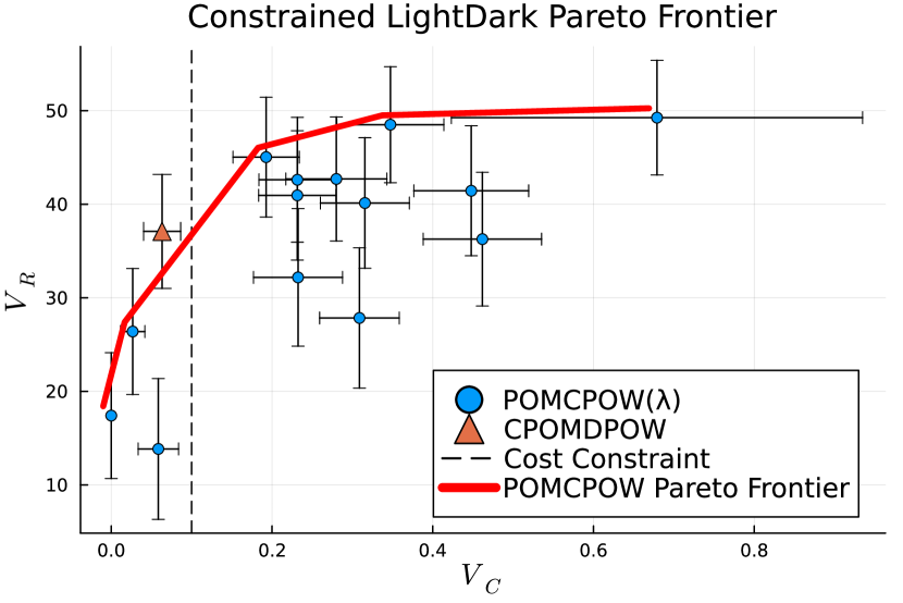
Figure 1: The $V_{R}$ vs. $V_{C}$ Pareto frontier of solutions to the scalarized LightDark POMDP solved with POMCPOW plotted on top of the Constrained LightDark CPOMDPOW solution. Error bars indicate standard deviation of the mean after 100 simulations.

First, we demonstrate the benefit of imposing hard constraints. To do so, we create an unconstrained LightDark problem by scalarizing the reward function and having an unconstrained solver optimize $\bar{R}(s,a)=R(s,a)-\lambda C(s,a)$. We then vary choices of $\lambda$ and compare the true reward and cost outcomes when using POMCPOW to solve the scalarized problem against using CPOMCPOW with the true CPOMDP.

In Figure 1, we depict the Pareto frontier of the soft-constrained problem when simulating 100 episodes for each choice of $\lambda$. We see that the solution to the constrained problem using CPOMCPOW lies above the convex hull while consistently satisfying the cost constraint. We can therefore see that constrained solvers can yield a higher reward value at a fixed cost while eliminating the need to search over scalarization parameters.

Cost propagation

Table 2: Statistics corresponding with actions $1$, $5$, and $10$ when running CPOMCPOW with normal cost propagation, minimal cost propagation, and on the unconstrained problem. $\Delta Q_{\lambda}$ denotes the gap to the best Lagrangian action-value, and the action taken most often is highlighted in red.

Model	${N(b_{0}a)/N(b_{0})}$	${Q_{c}(b_{0}a)}$	${\Delta Q_{\lambda}(b_{0}a)}$
Normal	$[0.10,0.19,0.08]$	$[0.18,0.32,1.15]$	$[-5.3,-5.5,-18.9]$
Min	$[0.14,0.33,0.18]$	$[0.00,0.00,0.29]$	$[-4.9,{\color[rgb]{1,0,0}-2.1},-4.3]$
Uncstr.	$[0.09,0.30,0.35]$	—	$[-8.9,-6.6,{\color[rgb]{1,0,0}-4.5}]$

Additionally, we simulate 50 CPOMCPOW searches from the initial LightDark belief with and without minimal cost propagation. In Table 2, we compare average statistics for taking actions $1$, $5$, and $10$ after each search has been completed. While in the unconstrained problem, the agent chooses the $10$ action to localize itself quickly, we note that the constrained agent should choose the $5$ action to carefully move towards the light region without overshooting and violating the cost constraint. We see that with normal cost propagation, the costs at the top level of the search tree are overly pessimistic, noting that actions of $1$ or $5$ should have $0$ cost-value as they are recoverable. We see that with normal cost propagation, this pessimistic cost-value distributes the search towards overly conservative actions, while with minimal cost propagation, the search focuses around and picks the $5$ action.

CPOMDP algorithm comparison

Table 1 compares mean rewards and costs received using CPOMCPOW, CPFT-DPW, and CPOMCP-DPW on the three target problems. Experimentation details are available in Appendix B. Crucially, our methods can generate desirable behavior while satisfying hard constraints without scalarization. This is especially evident in the Spillpoint problem, where setting hard constraints minimizes CO₂ leakage while improving the reward generated by unconstrained POMCPOW reported by Corso et al. (2022).

5 Conclusion

Planning under uncertainty is often multi-objective. Though multiple objectives can be scalarized into a single reward function with soft constraints, CPOMDPs provide a mathematical framework for POMDP planning with hard constraints. Previous work performs online CPOMDP planning for large state spaces, but small, discrete action and observation spaces by combining MCTS with dual ascent (Lee et al. 2018). We proposed algorithms that extend this to large or continuous action and observation spaces using progressive widening, demonstrating our solvers empirically on toy and real CPOMDP problems.

Limitations A significant drawback of CC-POMCP is that constraint violations are only satisfied in the limit, limiting its ability to be used as an anytime planner. This is worsened when actions and observations are continuous, as the progressive widening can miss subtrees of high cost. Finally, we note the limitation of using a single $\bm{\uplambda}$ to guide the whole search as different belief nodes necessitate different safety considerations.

Appendix A CPOMCP-DPW

Algorithm 3 CPOMCP-DPW

1:procedure Simulate($s$, $h$, $d$)

2:     if $d=0$ 

3:         return $0$      

4:     $new\leftarrow 0$

5:     $a\leftarrow\textsc{ActionProgWiden}(h)$

6:     if $|C(ha)|\leq k_{o}N(ha)^{\alpha_{o}}$ 

7:         $s^{\prime},o,r,\mathbf{c}\leftarrow G(s,a)$

8:         $C(ha)\leftarrow C(ha)\cup\{o\}$

9:         $M(hao)\leftarrow M(hao)+1$

10:         $\text{append }s^{\prime}\text{ to }B(hao)$

11:         if $M(hao)=1$ 

12:              $new\leftarrow 1$          

13:     else

14:         $o\leftarrow\text{select }o\in C(ha)\text{ w.p. }\frac{M(hao)}{\sum_{o}M(hao)}$

15:         $s^{\prime}\leftarrow\text{select }s^{\prime}\in B(hao)\text{ w.p. }\frac{1}{|B(hao)|}$

16:         $r\leftarrow R(s,a,s^{\prime})$

17:         $\mathbf{c}\leftarrow C(s,a,s^{\prime})$      

18:     if $new$ 

19:         $V^{\prime},\mathbf{C}^{\prime}\leftarrow\textsc{Rollout}(s^{\prime},hao,d-1)$

20:     else

21:         $V^{\prime},\mathbf{C}^{\prime}\leftarrow\textsc{Simulate}(s^{\prime},hao,d-1)$      

22:     $V\leftarrow r+\gamma V^{\prime}$

23:     $\mathbf{C}\leftarrow\mathbf{c}+\gamma\mathbf{C}^{\prime}$

24:     $N(h)\leftarrow N(h)+1$

25:     $N(ha)\leftarrow N(ha)+1$

26:     $Q(ha)\leftarrow Q(ha)+\frac{V-Q(ha)}{N(ha)}$

27:     $\mathbf{Q}_{C}(ha)\leftarrow\mathbf{Q}_{C}(ha)+\frac{\mathbf{C}-\mathbf{Q}_{C}(ha)}{N(ha)}$

28:     $\bar{\mathbf{c}}(ha)\leftarrow\bar{\mathbf{c}}(ha)+\frac{\mathbf{c}-\bar{\mathbf{c}}(ha)}{N(ha)}$

29:     if returnMinimalCost 

30:         $\mathbf{C}\leftarrow\underset{a\in C(h)}{\min}\,\mathbf{Q}_{C}(ha)$      

31:     return $V,\mathbf{C}$

Algorithm 3 outlines the straightforward application of double progressive widening to CC-POMCP (Lee et al. 2018). As noted by Sunberg and Kochenderfer (2018), this leads to rapid particle collapse in large or continuous observation spaces and performs similarly to a $Q_{\text{MDP}}$ policy, which assumes full observability in the next step.

Appendix B Experimentation Details

Experimentation settings, model parameters, belief updaters, solver hyperparameters, and default rollout policies are visible on our codebase at https://github.com/sisl/CPOMDPExperiments.

References

- Altman (1999) Altman, E. 1999. Constrained Markov Decision Processes, volume 7. CRC Press.
- Chaslot et al. (2008) Chaslot, G. M. J.-B.; Winands, M. H. M.; Herik, H. J. V. D.; Uiterwijk, J. W. H. M.; and Bouzy, B. 2008. Progressive strategies for Monte Carlo tree search. New Mathematics and Natural Computation, 4(03): 343–357.
- Corso et al. (2022) Corso, A.; Wang, Y.; Zechner, M.; Caers, J.; and Kochenderfer, M. J. 2022. A POMDP Model for Safe Geological Carbon Sequestration. In Advances in Neural Information Processing Systems (NeurIPS), Tackling Climate Change with Machine Learning Workshop.
- Couëtoux et al. (2011) Couëtoux, A.; Hoock, J.-B.; Sokolovska, N.; Teytaud, O.; and Bonnard, N. 2011. Continuous upper confidence trees. In International Conference on Learning and Intelligent Optimization (LION), 433–445. Springer.
- Egorov et al. (2017) Egorov, M.; Sunberg, Z. N.; Balaban, E.; Wheeler, T. A.; Gupta, J. K.; and Kochenderfer, M. J. 2017. POMDPs.jl: A Framework for Sequential Decision Making under Uncertainty. Journal of Machine Learning Research, 18(26): 1–5.
- Isom, Meyn, and Braatz (2008) Isom, J. D.; Meyn, S. P.; and Braatz, R. D. 2008. Piecewise Linear Dynamic Programming for Constrained POMDPs. In AAAI Conference on Artificial Intelligence (AAAI).
- Kim et al. (2011) Kim, D.; Lee, J.; Kim, K.-E.; and Poupart, P. 2011. Point-based value iteration for constrained POMDPs. In International Joint Conference on Artificial Intelligence (IJCAI).
- Kochenderfer, Wheeler, and Wray (2022) Kochenderfer, M. J.; Wheeler, T. A.; and Wray, K. H. 2022. Algorithms for Decision Making. MIT Press.
- Kurniawati, Hsu, and Lee (2008) Kurniawati, H.; Hsu, D.; and Lee, W. S. 2008. SARSOP: Efficient point-based pomdp planning by approximating optimally reachable belief spaces. In Robotics: Science and Systems.
- Lee et al. (2018) Lee, J.; Kim, G.-H.; Poupart, P.; and Kim, K.-E. 2018. Monte-Carlo tree search for constrained POMDPs. Advances in Neural Information Processing Systems (NeurIPS), 31.
- Lim, Tomlin, and Sunberg (2021) Lim, M. H.; Tomlin, C. J.; and Sunberg, Z. N. 2021. Voronoi Progressive Widening: Efficient Online Solvers for Continuous State, Action, and Observation POMDPs. In IEEE Conference on Decision and Control (CDC), 4493–4500.
- Mern et al. (2021) Mern, J.; Yildiz, A.; Sunberg, Z.; Mukerji, T.; and Kochenderfer, M. J. 2021. Bayesian optimized monte carlo planning. In AAAI Conference on Artificial Intelligence (AAAI), volume 35, 11880–11887.
- Piunovskiy and Mao (2000) Piunovskiy, A. B.; and Mao, X. 2000. Constrained Markovian decision processes: the dynamic programming approach. Operations Research Letters, 27(3): 119–126.
- Poupart et al. (2015) Poupart, P.; Malhotra, A.; Pei, P.; Kim, K.-E.; Goh, B.; and Bowling, M. 2015. Approximate linear programming for constrained partially observable Markov decision processes. In AAAI Conference on Artificial Intelligence (AAAI), volume 29.
- Roijers et al. (2013) Roijers, D. M.; Vamplew, P.; Whiteson, S.; and Dazeley, R. 2013. A survey of multi-objective sequential decision-making. Journal of Artificial Intelligence Research, 48: 67–113.
- Ross et al. (2008) Ross, S.; Pineau, J.; Paquet, S.; and Chaib-Draa, B. 2008. Online planning algorithms for POMDPs. Journal of Artificial Intelligence Research, 32: 663–704.
- Silver and Veness (2010) Silver, D.; and Veness, J. 2010. Monte-Carlo planning in large POMDPs. In Advances in Neural Information Processing Systems (NeurIPS), 2164–2172.
- Sondik (1978) Sondik, E. J. 1978. The optimal control of partially observable Markov processes over the infinite horizon: Discounted costs. Operations Research, 26(2): 282–304.
- Spaan and Vlassis (2005) Spaan, M. T.; and Vlassis, N. 2005. Perseus: Randomized point-based value iteration for POMDPs. Journal of Artificial Intelligence Research, 24: 195–220.
- Sunberg and Kochenderfer (2018) Sunberg, Z. N.; and Kochenderfer, M. J. 2018. Online algorithms for POMDPs with continuous state, action, and observation spaces. In International Conference on Automated Planning and Scheduling (ICAPS).
- Undurti and How (2010) Undurti, A.; and How, J. P. 2010. An online algorithm for constrained POMDPs. In IEEE International Conference on Robotics and Automation (ICRA), 3966–3973.
- Walraven and Spaan (2018) Walraven, E.; and Spaan, M. T. 2018. Column generation algorithms for constrained POMDPs. Journal of Artificial Intelligence Research, 62: 489–533.
- Wray and Czuprynski (2022) Wray, K. H.; and Czuprynski, K. 2022. Scalable gradient ascent for controllers in constrained POMDPs. In IEEE International Conference on Robotics and Automation (ICRA), 9085–9091.
- Wu et al. (2021) Wu, C.; Yang, G.; Zhang, Z.; Yu, Y.; Li, D.; Liu, W.; and Hao, J. 2021. Adaptive Online Packing-guided Search for POMDPs. Advances in Neural Information Processing Systems (NeurIPS), 34: 28419–28430.