Amoeba formulation of the non-Hermitian skin effect in higher dimensions

Abstract

The non-Hermitian skin effect dramatically reshapes the energy bands of non-Hermitian systems, meaning that the usual Bloch band theory is fundamentally inadequate as their characterization. The non-Bloch band theory, in which the concept of Brillouin zone is generalized, has been widely applied to investigate non-Hermitian systems in one spatial dimension. However, its generalization to higher dimensions has been challenging. Here, we develop a formulation of the non-Hermitian skin effect and non-Bloch band theory in arbitrary spatial dimensions, which is based on a natural geometrical object known as the amoeba. Our theory provides a general framework for studying non-Hermitian bands beyond one dimension. Key quantities of non-Hermitian bands, including the energy spectrum, eigenstates profiles, and the generalized Brillouin zone, can be efficiently obtained from this approach.

I Introduction

Non-Hermitian Hamiltonians have wide applications in many branches of physics, ranging from classical wave phenomena to open quantum systems Ashida et al. (2020); Bergholtz et al. (2021). Among various non-Hermitian systems, those have spatially periodic structures are especially important and extensively studied. Recently, their interplay with topological physics has stimulated the fruitful investigations of non-Hermitian topological states Bergholtz et al. (2021); Ding et al. (2022). One of the key phenomena uncovered in this direction is the non-Hermitian skin effect (NHSE), which refers to the counterintuitive feature that the nominally bulk eigenstates of a non-Hermitian Hamiltonian are strongly localized at the boundary Yao and Wang (2018); Kunst et al. (2018); Lee and Thomale (2019); Martinez Alvarez et al. (2018); Helbig et al. (2020); Xiao et al. (2020); Ghatak et al. (2020); Wang et al. (2022). Among other consequences, it implies that the energy spectrums of a non-Hermitian system can be drastically different under the experimentally-favored open boundary condition (OBC) and the theoretically-efficient periodic boundary condition (PBC). In sharp contrast to the Anderson localization, the NHSE-induced exponential localization can occur in pristine non-Hermitian systems without any disorder.

As a pronounced deviation from the usual Bloch-wave picture, the NHSE implies that the standard Bloch band theory is insufficient to characterize a generic non-Hermitian band. For example, the OBC energy spectrum cannot be calculated within this framework. To address this serious issue, a non-Hermitian generalization of the standard band theory, known as the non-Bloch band theory, has been introduced and applied to various non-Hermitian systems Yao and Wang (2018); Yokomizo and Murakami (2019); Lee and Thomale (2019); Longhi (2019, 2020); Kawabata et al. (2020); Yang et al. (2020a); Song et al. (2019a); Lee et al. (2020); Yi and Yang (2020). A central concept in this theory is the generalized Brillouin zone (GBZ), which is the proper surrogate for the conventional Brillouin zone (BZ) in Hermitian bands. The GBZ allows efficient computation of the continuous OBC energy spectrum of a large system without the need of diagonalizing a large Hamiltonian matrix in real space. Meanwhile, the shape of GBZ directly tells the information of real-space eigenstates, e.g., the skin localization lengths. Moreover, the topological invariants on GBZ are able to predict the number of topological boundary modes of non-Hermitian systems, for which the usual BZ-based topological numbers fails to deliver.

So far, the GBZ has been well defined only in one dimension (1D). Finding a general definition and formula for GBZ in two and higher dimensions is challenging, because the well-known 1D approach is not amenable to a straightforward generalization Yao and Wang (2018); Yokomizo and Murakami (2019); Wang . In certain special cases, the two-dimensional (2D) GBZ has been approximately defined and calculated Yao et al. (2018); Liu et al. (2019). However, a general approach without resorting to uncontrolled approximations has been lacking. Moreover, the recent finding of geometry-dependent NHSE in 2D non-Hermitian systems suggests that the GBZ might even not be definable in 2D Zhang et al. (2022).

In this paper, we present a general formulation of how the GBZ and related spectral concepts are quantitatively determined in two and higher dimensions. In 1D, our formulation reduces to the well-known GBZ formulation. The formulation is universal in the sense that our main results are applicable to models in arbitrary spatial dimensions, and with arbitrary degrees of freedom in a unit cell.

Our theory is based on a natural geometrical object called the amoeba by mathematicians Gelfand et al. (1994). Inspired by the amoeba and related mathematical tools, we formulate an amoeba-based theory which characterizes the NHSE quantitatively in arbitrary spatial dimensions. In particular, it is possible to directly calculate the energy spectrum and density of states (DOS) in the thermodynamic (i.e., large-size) limit without the troublesome finite-size errors. A rigorous theorem is proved as the general basis for DOS calculations. We also demonstrate, despite the geometry-dependent NHSE, the existence of a universal spectrum to which the OBC spectrum under a generic geometry converges. Furthermore, the amoeba inspires a definition and the associated algorithm of the GBZ in arbitrary spatial dimensions. Among other applications, this amoeba-based GBZ provides a starting point for calculating non-Bloch band topology beyond 1D.

The remainder of this article is arranged as follows. In Sec. II, we go through the existing method of determining the GBZ in 1D, and then try to find the clues for its higher-dimensional generalization. In Sec. III we introduce the basic mathematical properties of the amoeba and the associated Ronkin function which will be useful in calculating the DOS and the GBZ. In Secs. IV, V and VI we introduce the amoeba formulation for non-Hermitian systems, and then make use of this formulation and the theory of Toeplitz matrices to establish a universal way to determine the DOS as well as the GBZ. Non-Bloch band topology based on the proposed GBZ theory is studied in Sec. VII. Finally, in Sec. VIII, some useful inequalities on the OBC and PBC spectrums are proved from the amoeba approach.

II From generalized Brillouin zone to amoeba

We start with reviewing the concept of generalized Brillouin zone (GBZ) in 1D Yao and Wang (2018); Yokomizo and Murakami (2019); Yang et al. (2020b); Zhang et al. (2020), searching for clues of its higher-dimensional generalizations.

A general 1D tight-binding Hamiltonian with OBC can be written as

$$H=\sum_{i,j=1}^{L}\sum_{a,b}\left|i,a\right\rangle\left(t_{j-i}\right)_{ab}\left\langle j,b\right|,$$ (1)

where $i,j$ are the position indices, and $a,b$ are the indices for intra-cell degrees of freedom (band indices). When the hopping matrix $t_{j-i}$ depends only on the spatial distance $j-i$, we have translational symmetry in the bulk. The Hermiticity condition $t_{n}=t_{-n}^{\dagger}$ is not required since non-Hermitian Hamiltonians are our focus. A finite hopping range $n_{c}$ is taken so that the hopping matrix $t_{n}=0$ when $|n|>n_{c}$. Given this real-space Hamiltonian, the corresponding Bloch Hamiltonian is the Fourier transform of $t_{n}$:

$$h(e^{ik})=\sum_{n}t_{n}\left(e^{ik}\right)^{n}.$$ (2)

Note that the Bloch Hamiltonian has been written as $h(e^{ik})$ instead of the more frequently used $h(k)$. This simplifies our notations when the real-valued wave vector $k$ is generalized to the complex plane, which amounts to making the substitution $e^{ik}\rightarrow e^{\mu+ik}=\beta$ ($k$ and $\mu$ are real-valued). Apparently, $h(\beta)=\sum_{n}t_{n}\beta^{n}$ is a matrix-valued Laurent polynomial of $\beta$.

To solve the real-space Schrödinger equation $H\left|\psi\right\rangle=E\left|\psi\right\rangle$, it is standard to take the superposition of exponential functions $|\psi\rangle=\sum_{n,a}c_{n,a}(\beta_{n})^{j}|j,a\rangle$, where all $\beta_{n}$’s satisfy the characteristic equation

$$\det[E-h(\beta)]=0,$$ (3)

and the coefficients $c_{n,a}$ are to be determined by the boundary conditions. We expand the characteristic polynomial as $\det[E-h(\beta)]=a_{-M}\beta^{-M}+\dots+a_{N}\beta^{N}$ with $a_{M}$, $a_{N}$ nonzero, and order the solutions of Eq. (3) as $|\beta_{1}(E)|\leq|\beta_{2}(E)|\leq\dots\leq|\beta_{M+N}(E)|$. It has been found that, in the thermodynamic (large-size) limit, the OBC continuous spectrum is determined by the following simple equation Yao and Wang (2018); Yokomizo and Murakami (2019); Zhang et al. (2020):

$$\left|\beta_{M}(E)\right|=\left|\beta_{M+1}(E)\right|.$$ (4)

Notably, the size $L$ does not appear in this equation. Since $\beta_{M}$, $\beta_{M+1}$ and $E$ are mutually related by the characteristic equation, there is only one complex-valued unknown, i.e., two real-valued unknowns, in Eq. (4). Since Eq. (4) imposes a single real-valued constraint, the solution space is one-dimensional. We may view $\beta_{M}$ or $\beta_{M+1}$ as the unknown in Eq. (4). It turns out that all the $\beta_{M},\beta_{M+1}$ solutions on the complex $\beta$ plane form a one-dimensional closed curve. This curve is known as the GBZ, which contains the key information about the eigenstate profiles, including the conventional wave vector $k$ and the spatial decay rate $\mu$ of a skin mode. Solving $E$ from Eq. (3), with $\beta$ varying in the GBZ, yields the OBC energy spectrums. Furthermore, the topological boundary modes are dictated by the topological invariants defined in the GBZ rather than in the Brillouin zone (BZ), which is dubbed the non-Bloch bulk-boundary correspondence Yao and Wang (2018); Yokomizo and Murakami (2019). Thus, in many senses, GBZ plays a similar role as BZ does in Hermitian physics. The band theory based on the GBZ concept is known as the non-Bloch band theory.

To demonstrate the applications of non-Bloch band theory, we consider the non-Hermitian Su-Schrieffer-Heeger (SSH) model with the Bloch Hamiltonian Yao and Wang (2018); Kunst et al. (2018):

$$h(e^{ik}) = [t_{1}+(t_{2}+t_{3})\cos k]\sigma_{x}$$ (5)

$$+[(t_{2}-t_{3})\sin k+i\dfrac{\gamma}{2}]\sigma_{y},$$

or, in terms of $\beta$,

$$h(\beta) = [t_{1}+\frac{t_{2}+t_{3}}{2}(\beta+\frac{1}{\beta})]\sigma_{x}$$ (6)

$$+[\frac{t_{2}-t_{3}}{2i}(\beta-\frac{1}{\beta})+i\dfrac{\gamma}{2}]\sigma_{y},$$

where $\sigma_{x,y,z}$ are the Pauli matrices. It is known that the eigenstates exhibit NHSE under OBC, and consequently, the OBC and PBC energy spectrums are drastically different Yao and Wang (2018); Kunst et al. (2018). As an illustration, the OBC and PBC spectrums are plotted in Fig. 1(a), for parameter values $t_{1}=t_{2}=1$, $t_{3}=0.7$, and $\gamma=4/3$. This choice of parameters is in the topologically nontrivial regime, and therefore topological edge modes with $E=0$ is found in the OBC energy spectrum. The characteristic equation, Eq. (3), is a quartic equation of $\beta$, and its four solutions are shown in Figs. 1(b) and (c), for $E=E_{1}=-1+0.3i$ and $E=E_{2}=-1$, respectively. Instead of $\beta$ itself, we show $\mu=\log|\beta|$, namely the imaginary part of the wave vector. As stated in Eq. (4), when and only when $\left|\beta_{2}(E)\right|=\left|\beta_{3}(E)\right|$, i.e., $\mu_{2}(E)=\mu_{3}(E)$, will $E$ belong to the OBC energy spectrum. This is the case for $E=E_{2}$ [Figs. 1(c)]. The corresponding $\beta_{2}(E_{2})$ and $\beta_{3}(E_{2})$ belong to the GBZ.

Remarkably, the GBZ equation, Eq. (4), enables us to find the OBC energy spectrums and other physical quantities without the need of diagonalizing a large real-space Hamiltonian whose size grows with the system size. The thermodynamic-limit quantities are obtained directly from the GBZ equation. A natural question arises: What is the higher-dimensional counterpart of Eq. (4)?

To be concrete, we consider a single-band model shown in Fig. 2(a). With the notation $\bm{\beta}=(\beta_{x},\beta_{y})=(e^{ik_{x}},e^{ik_{y}})$, the corresponding Bloch Hamiltonian is

$$h(\bm{\beta}) =t\left(\beta_{x}+\beta_{x}^{-1}+\beta_{y}+\beta_{y}^{-1}\right)$$

$$\phantom{=}+t^{\prime}\left(\beta_{x}+\beta_{x}^{-1}\right)\left(\beta_{y}+\beta_{y}^{-1}\right)$$

$$\phantom{=}+\gamma\left(\beta_{x}-\beta_{x}^{-1}+\beta_{y}-\beta_{y}^{-1}\right),$$ (7)

For concreteness, we shall fix parameter values $t=1$, $t^{\prime}=0.5$, and $\gamma=0.2$. The numerical energy spectrums from brute-force diagonalization are shown in Figs. 1(d).

We hope to generalize the non-Bloch band theory to 2D, such that the energy spectrum can be obtained from the GBZ instead of the real space. The characteristic equation takes the same form as in 1D (and the reasoning is also the same):

$$\det[E-h(\bm{\beta})]=0.$$ (8)

For our single-band model, the determinant can be dropped, and the characteristic equation is simply $E-h(\bm{\beta})=0$. Notably, the zero locus of $\det[E-h(\bm{\beta})]$, namely the $\bm{\beta}$-solution space of $\det[E-h(\bm{\beta})]=0$, is (real) two-dimensional. In fact, the solution space can be locally parameterized by the complex-valued $\beta_{x}$ or $\beta_{y}$, one of which is determined by the other via the characteristic equation. In contrast, the zero locus of $E-h(\beta)$ for a 1D system is zero-dimensional, that is several isolated $\beta$ points.

The next step, following the approach in the 1D non-Bloch band theory, is to select the legitimate $\beta$’s by adding the boundary conditions. For 1D systems with OBC, the number of constraint equations imposed by the boundary condition does not grow with the system size $L$, which greatly simplifies the derivation of GBZ equation, Eq. (4) Yao and Wang (2018); Yokomizo and Murakami (2019). For 2D OBC systems (e.g., with square or disk geometry), however, the number of constraint equations is proportional to the linear size $L$. It is therefore challenging to exploit all these boundary-condition equations. Consequently, it is difficult to obtain a 2D counterpart of Eq. (4) from the approach similar to 1D.

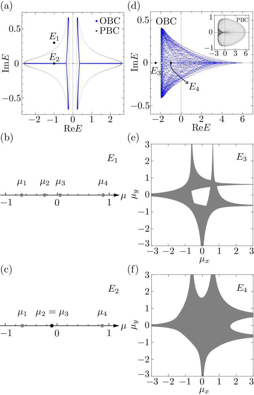
Figure 1: Energy spectrums and amoebae. (a) Energy spectrum of the 1D non-Hermitian SSH model Eq. (6) for a chain with length $L=300$, under OBC (blue) and PBC (gray), respectively. Parameter values are $t_{1}=t_{2}=1$, $t_{3}=0.7$, and $\gamma=4/3$. (b)(c) Illustrations of $\mu=\log|\beta|$, where $\beta$ satisfies the 1D characteristic equation $\det[E-h(\beta)]=0$. $E$ is taken to be $E_{1}=-1+0.3i$ in (b), and $E_{2}=-1$ in (c). For $E_{2}$ belonging to the OBC spectrum, we have $\mu_{2}(E_{2})=\mu_{3}(E_{2})$. (d) Energy spectrum of the 2D model Eq. (II). Main figure: Disk geometry (OBC) with diameter $L=140$. Inset: Torus geometry (PBC). Parameter values are $t=1$, $t^{\prime}=0.5$, and $\gamma=0.2$. (e)(f) Illustrations of the 2D amoebae whose points are $(\mu_{x},\mu_{y})=(\log|\beta_{x}|,\log|\beta_{y}|)$, where $\bm{\beta}$ satisfies the 2D characteristic equation $\det[E-h(\bm{\beta})]=0$ of the model Eq. (II). $E_{3}=-2.5$ in (e), and $E_{4}=-1$ in (f). Notably, there is a hole in the amoeba for $E_{3}$ outside the OBC spectrum, and no hole for $E_{4}$ in the OBC spectrum.

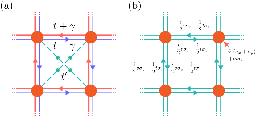
Figure 2: Illustration of the real-space Hamiltonian of 2D models. (a) Single band toy model Eq. (II). (b) The non-Hermitian Chern-band model Eq. (VII). All the parameters $t,\gamma,v,m$ are real-valued.

Although a straightforward generalization to 2D looks infeasible, we can still find some clues from the 1D GBZ construction. Eq. (4) and Figs. 1(b)(c) suggest that the moduli of the solutions to the characteristic equation contain much useful information about the energy spectrum. We correspondingly plot the solutions to the 2D characteristic equation, followed by mapping $(\mu_{x},\mu_{y})=(\log|\beta_{x}|,\log|\beta_{y}|)$, in Figs. 1(e)(f). This geometrical object is known as the amoeba in mathematics literature (see Sec. III for a brief introduction) Gelfand et al. (1994); Viro (2002); Forsberg et al. (2000); Theobald (2002); Rullgård (2001). We notice that a hole exists in the amoeba in Fig. 1(e), for which the energy $E_{3}$ does not belong to the OBC spectrum. In contrast, there is no hole in the amoeba in Fig. 1(f), with energy $E_{4}$ belonging to the OBC spectrum. Viewed from this amoeba perspective, 1D non-Hermitian energy spectrums also exhibit similar behaviors. In 1D, the amoeba consists of discrete points, and the hole is simply the open interval between two adjacent points. For example, the open interval $(\mu_{2},\mu_{3})$ in Fig. 1(b) can be viewed as a hole, which closes in Fig. 1(c) with $\mu_{2}=\mu_{3}$.

From the above examples, we observe that the absence (presence) of a hole in the amoeba of the characteristic polynomial could be an indicator of the energy $E$ being (being not) in the OBC energy spectrum. This is a key observation of the present work. To obtain more quantitative results from this observation, it is helpful to know some mathematical properties about the amoeba.

III Mathematical properties of amoeba and Ronkin function

In this section, we shall introduce the basic concept of amoeba and a closely related analytic tool, the Ronkin function. As a quite recent concept in mathematics, the amoeba was introduced by Gelfand, Kapranov, and Zelevinsky in 1994 Gelfand et al. (1994). Albeit elementary, the notion of amoeba has deep connections to various algebro-geometric concepts, which stimulated extensive studies in mathematics Viro (2002); Forsberg et al. (2000); Theobald (2002); Rullgård (2001).

Let $f$ be a Laurent polynomial of $\beta_{j}$, $j=1,2,\dots,d$, where $d$ will be identified as the spatial dimension in our study. The amoeba of $f$ is defined as the log-moduli of the zero locus of $f$

$$\mathcal{A}_{f}=\left\{\log\left|\bm{\beta}\right|:f(\bm{\beta})=0\right\}\subset\mathbb{R}^{d},$$ (9)

in which we have used the notation $\log|\bm{\beta}|=(\log|\beta_{1}|,\dots,\log|\beta_{d}|)$ to simply the expression. Similar notations such as $e^{\bm{\mu}}=(e^{\mu_{1}},\dots,e^{\mu_{d}})$ will be used hereafter. In our case, the Laurent polynomial in use is $\det[E-h(\bm{\beta})]$. We can see that the geometric objects in Figs. 1(b)(c) and (e)(f) are 1D and 2D amoebae, respectively.

The name of amoeba was motivated by its shape in 2D: It has slim “tentacles” extending to infinity, and sometimes several “vacuoles” (holes) inside its body. Intriguingly, these holes will play important roles in our theory. It is known that the amoeba in any spatial dimensions is a closed set, and each hole is a convex set Forsberg et al. (2000).

A useful analytic tool in the study of amoeba is the Ronkin function, which is defined as Viro (2002); Passare and Rullgard (2004); Ronkin (1974):

$$R_{f}(\bm{\mu})=\int_{T^{d}}\left(\dfrac{d\theta}{2\pi}\right)^{d}\log\left|f(e^{\bm{\mu}+i\bm{\theta}})\right|,$$ (10)

where the domain of integration is the $d$-dimensional torus $T^{d}=[0,2\pi]^{d}$, and the expression has been simplified by the notations $f(e^{\bm{\mu}+i\bm{\theta}})=f(e^{\mu_{1}+i\theta_{1}},\cdots,e^{\mu_{d}+i\theta_{d}})$, and $(\frac{d\theta}{2\pi})^{d}=\frac{d\theta_{1}}{2\pi}\dots\frac{d\theta_{d}}{2\pi}$.

It is helpful to take the gradient of the Ronkin function Forsberg et al. (2000); Passare and Rullgard (2004). To this end, we can express the integrand in $R_{f}$ as $\log|f|=\operatorname{Re}(\log f)$. The real part can be taken at the end of the calculation. It turns out that the integral is real-valued before taking the real part, and therefore the “$\operatorname{Re}$” symbol can be discarded. The derivation proceeds as

$$\nu_{j} = \frac{\partial R_{f}(\bm{\mu})}{\partial\mu_{j}}$$ (11)

$$= \operatorname{Re}\int_{T^{d}}\left(\dfrac{d\theta}{2\pi}\right)^{d}\partial_{\mu_{j}}\log f(e^{\bm{\mu}+i\bm{\theta}})$$

$$= \operatorname{Re}\int_{T^{d}}\left(\dfrac{d\theta}{2\pi}\right)^{d}\frac{\partial_{\mu_{j}}f(e^{\bm{\mu}+i\bm{\theta}})}{f(e^{\bm{\mu}+i\bm{\theta}})}$$

$$= \operatorname{Re}\int_{T^{d}}\left(\dfrac{d\theta}{2\pi}\right)^{d}\frac{-i\partial_{\theta_{j}}f(e^{\bm{\mu}+i\bm{\theta}})}{f(e^{\bm{\mu}+i\bm{\theta}})}.$$

In the last line we used $\partial_{\mu_{j}}=-i\partial_{\theta_{j}}$ acting on $f$. We observe that

$$w_{j} = \frac{1}{2\pi i}\int_{0}^{2\pi}d\theta_{j}\frac{\partial_{\theta_{j}}f(e^{\bm{\mu}+i\bm{\theta}})}{f(e^{\bm{\mu}+i\bm{\theta}})}$$ (12)

is the winding number of the phase of $f$ along a circle parameterized by $\theta_{j}$, so it is always real-valued. Thus, the gradient $\nu_{j}$ is the average of the winding number $w_{j}$ on the $(d-1)$-dimensional torus parameterized by $(\theta_{1},\cdots,\theta_{j-1},\theta_{j+1},\cdots,\theta_{d})$:

$$\nu_{j}=\int_{T^{d-1}}\frac{d\theta_{1}\cdots d\theta_{j-1}d\theta_{j+1}\cdots d\theta_{d}}{(2\pi)^{d-1}}w_{j}.$$ (13)

For example, in 2D, one has $\nu_{1}=\int_{0}^{2\pi}\frac{d\theta_{2}}{2\pi}w_{1}$ and $\nu_{2}=\int_{0}^{2\pi}\frac{d\theta_{1}}{2\pi}w_{2}$.

The Ronkin function is linear in the complement of the amoeba. In fact, when $\bm{\mu}$ is not in the amoeba, $f(e^{\bm{\mu}+i\bm{\theta}})\neq 0$ is satisfied in the entire $T^{d}$ parameterized by $(\theta_{1},\cdots,\theta_{d})$. It follows that $w_{j}$ is an integer-valued constant as $\{\theta_{1},\cdots,\theta_{j-1},\theta_{j+1},\cdots,\theta_{d}\}$ are varied, and therefore the average, $\nu_{j}$, is the same integer constant. Thus, we can assign to each amoeba hole an integer-valued vector $\bm{\nu}=(\nu_{1},\dots,\nu_{d})$, dubbed the order of the hole. The orders of two different holes cannot be equal Forsberg et al. (2000). Crucially, there exists at most one hole with order $\bm{\nu}=(0,\cdots,0)$, which is called the central hole. Because the order is zero, the Ronkin function is a constant in this hole. Moreover, the Ronkin function is convex in the entire $\bm{\mu}$ space, i.e., $R_{f}(\lambda\bm{\mu}_{1}+(1-\lambda)\bm{\mu}_{2})\leq\lambda R_{f}(\bm{\mu}_{1})+(1-\lambda)R_{f}(\bm{\mu}_{2})$ is satisfied for any two points $\bm{\mu}_{1,2}$ and $0<\lambda<1$ Viro (2002); Passare and Rullgard (2004). An easy corollary of the convexity is that a Ronkin function converges everywhere: if it is $-\infty$ at one point, convexity would conclude that it is $-\infty$ everywhere.

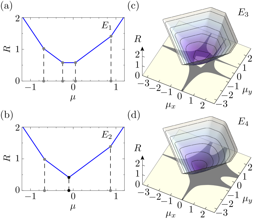
Figure 3: The Ronkin function in (a,b) 1D and (c,d) 2D, taken at energies (a) $E_{1}$, (b) $E_{2}$, (c) $E_{3}$, and (d) $E_{4}$ stated in Fig. 1. For (a)(b), the Laurent polynomial is Eq. (6); for (c)(d), it is Eq. (II). The parameter values are the same as stated in Fig. 1. In both 1D and 2D, the Ronkin function is strictly linear on each component (hole) of the complement of the amoeba, where the gradient equals the integer index. The Ronkin function is always convex. In consequence, when the central hole exists, the minimum is reached on the central hole; otherwise, the minimum is reached at a single point in the amoeba.

In 1D, the Ronkin function is closely related to the famous Jensen’s formula, which reads Stein and Shakarchi (2010)

$$\dfrac{1}{2\pi}\int_{0}^{2\pi}d\theta\,\log\left|g\left(Re^{i\theta}\right)\right|=\log\left|g(0)\right|+\sum_{k=1}^{l}\log\left|\dfrac{R}{z_{k}}\right|,$$ (14)

where $g$ is a holomorphic function with $g(0)\neq 0$, and $z_{k}$ ($k=1,\cdots,l$) are the zeros of $g$ enclosed by the circle $|\beta|=R$. Jensen’s formula can be readily obtained from Eq. (11) with $d=1$, in which case the gradient $\nu=w$ (the index $j=1$ is redundant). In fact, the left-hand side of Eq. (14) is exactly the Ronkin function $R_{g}(\log|R|)$. To calculate it, we order the zeros of $g$ as $|z_{1}|\leq|z_{2}|\leq|z_{3}|\leq\cdots$. According to Eq. (11) and Eq. (12), the gradient $\nu=\frac{\partial R_{g}}{\partial(\log|R|)}$ equals to the winding number of $g$ along the circle $|\beta|=R$, which counts the number of enclosed zeros. Therefore, we have $\nu=0$ for $\log|R|<\log|z_{1}|$, and $\nu=k$ for $\log|z_{k}|<\log|R|<\log|z_{k+1}|$. It follows that, when the circle $|\beta|=R$ encloses $l$ zeros,

$$R_{g}(\log|R|) = \log|g(0)|+\log\frac{|z_{2}|}{|z_{1}|}+2\log\frac{|z_{3}|}{|z_{2}|}+3\log\frac{|z_{4}|}{|z_{3}|}$$ (15)

$$+\cdots+l\log\frac{|R|}{|z_{l}|},$$

$$= \log\left|g(0)\right|+\sum_{k=1}^{l}\log\left|\dfrac{R}{z_{l}}\right|,$$

which is exactly Jensen’s formula Eq. (14).

We now apply the explicit formula of Ronkin function to $\det[E-h(\beta)]=a_{-M}\beta^{-M}+\dots+a_{N}\beta^{N}$ whose zeros are $|\beta_{1}|\leq|\beta_{2}|\leq\dots\leq|\beta_{M+N}|$. We rewrite it as $\det[E-h(\beta)]=f(\beta)g(\beta)$ with $f(\beta)=a_{-M}\beta^{-M}$, so that $g(\beta)$ has no pole in the complex plane and $g(0)=1$. Applying Eq. (15) to $g$, we have

$$R_{\det(E-h)}(\mu) = R_{f}(\mu)+R_{g}(\mu)$$

$$= \log|a_{-M}|-M\mu+\sum_{k=1}^{l}(\mu-\log|\beta_{k}|),$$

for $|\beta_{l}|\leq e^{\mu}\leq|\beta_{l+1}|$. Thus, $R_{h}$ is a piecewise linear function of $\mu$ in 1D. Each zero $|\beta_{k}|$ is an amoeba component, and each open interval $(|\beta_{k}|,|\beta_{k+1}|)$ is an amoeba hole. The central hole with order $\nu=\frac{\partial R_{h}}{\partial\mu}=0$, in which the Ronkin function is flat (being a constant), is the open interval $(|\beta_{M}|,|\beta_{M+1}|)$. Therefore, Eq. (4) means that an energy $E$ belongs to the OBC bulk spectrum when the central hole shrinks to zero size. Thus, the Ronkin function provides crucial information about the energy spectrums. Fig. 3 (a)(b) are two examples of the 1D Ronkin function. The Ronkin function is flat in the central hole of Fig. 3 (a) corresponding to $E$ outside the energy spectrum, and the hole shrinks to a point in Fig. 3 (b) corresponding to $E$ belonging to the energy spectrum.

In 2D and higher dimensions, it is challenging to obtain a closed form for the Ronkin function. Nevertheless, regardless of the spatial dimensions, the Ronkin function is always globally convex, and is linear in the amoeba holes (i.e. the complement of amoeba). If there is a central hole, the Ronkin function takes minimum in the entire hole, namely, the function has a flat bottom in this hole [Fig. 3 (c)]; otherwise, the Ronkin minimum is reached at a single point in the amoeba [Fig. 3 (d)].

In view of the aforementioned relation between the GBZ and Ronkin function in 1D, it is natural to ask whether there is a deep connection between the non-Hermitian energy spectrums and the Ronkin function in higher dimensions. In fact, we have already seen some numerical clues for such a connection. Our observation about 2D non-Hermitian systems at the end of Sec. II can be rephrased in terms of the Ronkin function: If and only if the minimum of the Ronkin function $R_{\det(E-h)}$ is reached at a single point $\bm{\mu}_{\min}(E)$, instead of in a hole with nonzero size, will $E$ be in the OBC bulk spectrum.

In 1D, the single point where the Ronkin function takes the minimum is $\mu_{\min}(E)=\log|\beta_{M}(E)|=\log|\beta_{M+1}(E)|$. Note that $|\beta_{M}(E)|=|\beta_{M+1}(E)|$ is the decay factor of an OBC eigenstate. Thus, the location of the minimum of Ronkin function precisely determines the decay factor of an OBC eigenstate. In other words, the Ronkin function tells the shape of the GBZ. We propose that this reformulation of GBZ in terms of Ronkin function is generalizable to non-Hermitian systems in higher dimensions, which will be justified in the following sections.

IV Energy Spectrums and density of states

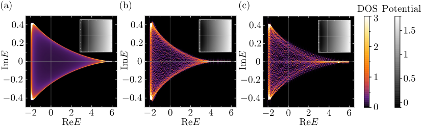
Figure 4: Density of states (DOS) from the Ronkin function and diagonalization of real-space Hamiltonian. The Hamiltonian used here is Eq. (II) [Fig. 2(a)], with parameter values $t=1$, $t^{\prime}=0.5$, and $\gamma=0.2$. (a) DOS from the Ronkin function, via Eq. (21). (b) DOS from diagonalizing the real-space Hamiltonian on a square with side length $L=130$. An on-site random potential distributed uniformly in $[-0.5,0.5]$ is added at each boundary site. (c) DOS from diagonalizing of real-space Hamiltonian on a disk with diameter $L=140$ (without random potential at the boundary). The inset show the Coulomb potential, $\phi(E)$ in (a), and $\Phi(E)$ in (b) and (c). To facilitate comparison with (a), the DOS in (b) and (c) is also obtained from the Coulomb potential via Eq. (18), in which $\Phi(E)$ is generated by diagonalizing the real-space Hamiltonian.

We now introduce the amoeba formulation of non-Hermitian energy bands in $d$ spatial dimensions. It is our purpose to calculate the energy spectrums and density of states (DOS), the number of states per area on the complex energy plane, in the thermodynamic limit. Note that when talking about the DOS, only bulk states are relevant, because the contribution from edge states fades away in the thermodynamic limit.

To describe the DOS of complex energy, it is convenient to use the language of electrostatics. Let us assign electric charge $-1/N$ to each energy eigenvalue $\epsilon_{n}$, where $N$ is the total number of unit cells (in this convention the total charge sums up to the number of energy bands, which is independent of the size $N$). In terms of Dirac’s $\delta$ function, the DOS of complex energy can be written as $\rho(E)=\lim_{N\rightarrow\infty}\sum_{n}\frac{1}{N}\delta(E-\epsilon_{n})$, which is just the absolute value of electric charge density.

Given the electric charge, the corresponding Coulomb potential $\Phi(E)$ is given by

$$\Phi(E) =\dfrac{1}{N}\sum_{\epsilon_{n}}\log\left|E-\epsilon_{n}\right|$$

$$\xrightarrow[N\to\infty]{}\int d^{2}E^{\prime}\,\log\left|E-E^{\prime}\right|\rho(E^{\prime}).$$ (17)

Conversely, the DOS, or the absolute value of charge density in the electrostatics language, can be readily obtained from the Coulomb potential by taking Laplacian,

$$\rho(E)=\dfrac{1}{2\pi}\Delta\Phi(E),$$ (18)

where $\Delta=\frac{\partial^{2}}{\partial(\operatorname{Re}E)^{2}}+\frac{\partial^{2}}{\partial(\operatorname{Im}E)^{2}}$ and the $N\to\infty$ limit is taken for $\Phi(E)$.

One of our main proposals is that the Coulomb potential $\Phi(E)$, in the $N\rightarrow\infty$ limit, can be obtained from the Ronkin function,

$$\Phi(E)=\phi(E),$$ (19)

where $\phi(E)$ is the minimum of Ronkin function of $\det(E-h)$ by varying $\bm{\mu}$,

$$\phi(E)=\min_{\bm{\mu}}R_{\det(E-h)}\left(\bm{\mu}\right).$$ (20)

Therefore, the DOS can be directly obtained from the Ronkin function,

$$\rho(E)=\dfrac{1}{2\pi}\Delta\phi(E).$$ (21)

In the special cases that the spectrum is a 1D object consisting of lines or curves in the complex energy plane, it is more preferable to define the DOS as states per length rather than states per area. In fact, the states per area will diverge in these cases, while states per length is in general finite. This is the case for 1D non-Hermitian lattice systems, and higher-dimensional systems with real spectrum. In a small neighborhood of a segment of the 1D spectrum, suppose that $\bm{n}$ is a normal vector to the segment. From the electrostatic analogy and Eq. (21), it is easy to see that the DOS per length, denoted by $\rho_{\mathrm{1D}}$, is given by

$$\rho_{\mathrm{1D}}=\dfrac{1}{2\pi}\left|\left(\dfrac{\partial\phi}{\partial\bm{n}}\right)_{+}-\left(\dfrac{\partial\phi}{\partial\bm{n}}\right)_{-}\right|,$$ (22)

where the two derivatives are taken on opposite sides of the curve segment.

Before diving into the sophisticated analytic approach, we provide numerical evidence for the Ronkin-function-based formula, Eq. (21). We take the model Eq. (II) [Fig. 2(a)] as an example. In Fig. 4, we numerically compare the DOS derived from the Ronkin function, via Eq. (21), and that from diagonalizing the OBC Hamiltonian. When implementing Eq. (21), the potential $\phi(E)$ and the discrete Laplacian are evaluated by discretizing the complex energy plane into grid points, so that the $\log$-divergence of a point-source potential is effectively blurred. The DOS obtained from the Ronkin function agrees well with those from real-space Hamiltonian, though there are some differences that can be naturally attributed to the finite-size nature of the real-space calculations. First, the spectrums from real-space diagonalization in Figs. 4(b) and (c) are slightly narrower in the $\operatorname{Im}E$-direction than the one derived from the Ronkin function in Fig. 4(a). Second, the eigenvalues from real-space diagonalization seem more likely to concentrate on the real axis. These differences can be explained by the non-Bloch PT symmetry, which is a unique size dependence of non-Hermitian spectrums in two and higher dimensions Song et al. (2022). In fact, our real-space Hamiltonian [see Eq. (II) and Fig. 2(a)] has real-valued hoppings and therefore commutes with the complex conjugation operator: $[H,\mathcal{K}]=0$. Combined with the NHSE, it means that the model has non-Bloch PT symmetry, which implies real energy spectrums when the size is small. As the size $L$ grows to infinity, the proportion of real eigen-energies diminishes to zero Song et al. (2022). Since the length $L$ adopted in Fig. 4(b) and (c) is finite, the PT symmetry breaking is incomplete, leaving a nonzero proportion of real eigen-energies.

We emphasize that the Ronkin function tells the universal spectrum and universal DOS of the OBC system, the precise meaning of which we will explain below. It is clear that the amoeba and the Ronkin function do not contain information about the shape (e.g., square or disk) or boundary details (e.g., clean or locally perturbed) of the OBC system. The Ronkin function yields the same DOS regardless of these geometrical details. Therefore, this approach per se assumes a detail-independent (therefore universal) spectrum with a universal DOS, which is supported by our numerical calculations. In fact, our numerical results indicate that the DOS of an OBC system with an arbitrary shape converges in the large-size limit to the same universal DOS, at least when certain random local perturbations are added to the boundary [e.g., in Fig. 4(b)]. Note that the DOS thus obtained is independent of the specific forms of boundary randomness . In generic cases, even the boundary randomness is not necessary to ensure the convergence to the universal DOS. For example, the DOS of disk geometry without boundary random potential already resembles the universal DOS [Fig. 4(c)]. In contrast, for a polygon geometry (e.g., a square), boundary randomness significantly helps the DOS to converge to the universal DOS. Without the boundary randomness, the polygon geometry can exhibit the geometry-dependent non-Hermitian skin effect, by which different polygons may have different DOS Zhang et al. (2022). Our intuitive understanding of this phenomenon is as follows. The boundary of a polygon consists of straight line segments, which are perfectly reflective in the sense that the wavevector (momentum) parallel to the line segment is conserved during wave reflection. Thus, the boundary fails to fully mix waves with different wavevectors and therefore the Hamiltonian can be viewed as fine-tuned rather than generic. As such, the spectrum exhibits the fingerprint of specific geometry rather than the universal spectral properties of the Hamiltonian. Boundary or bulk randomness breaks the wavevector conservation and couples waves with different wavevectors, which generates a more generic energy spectrum. An analogous phenomenon is the critical non-Hermitian skin effect in 1D Li et al. (2020); Yokomizo and Murakami (2021). In the zero-coupling limit of two coupled 1D chains, the straightforward application of the GBZ equation, Eq. (4), does not yield the correct OBC energy spectrum . The zero-coupling limit represents a fine-tuned point, and a small inter-chain coupling brings the spectrum to that predicted by the GBZ theory Li et al. (2020); Yokomizo and Murakami (2021). In 2D, our numerical results suggest that the Hamiltonian should be viewed as fine-tuned for polygon shapes, and a small randomness restores the universal spectrum characterized by the universal DOS.

To summarize, there exists a geometry-independent universal spectrum that can be calculated from the amoeba and Ronkin function. The DOS of an OBC system with a generic shape always approaches the universal DOS in the large-size limit. When the DOS of an (non-generic) OBC system with a certain shape appears to deviate from the universal DOS, this difference can be eliminated by adding a small random local perturbation. From an experimental point of view, the universal spectrum is particularly significant because disorders are often unavoidable in realistic systems.

We will establish the proposal Eq. (21) in a few steps. We begin with the Szegö’s limit theorem for the determinant of a large Toeplitz matrix. Before doing so, it is appropriate here to introduce the terminology of Toeplitz matrices Böttcher and Silbermann (1999); Böttcher and Grudsky (2005). A matrix $A$ determined by $A_{ij}=a_{j-i}$ is called a Toeplitz matrix, i.e., the matrix element $A_{ij}$ depends on the difference $j-i$ only. It is associated with an symbol, which is a complex-valued function $\sigma(e^{i\theta})=\sum_{n}a_{n}e^{in\theta}$ ($\theta\in[0,2\pi]$). A Toeplitz matrix is often expressed in terms of its symbol as $A=\mathcal{T}[\sigma]$. By definition, the elements of a Toeplitz matrix are the Fourier components of the symbol:

$$\mathcal{T}[\sigma]_{j_{1}j_{2}}=\int_{0}^{2\pi}\frac{d\theta}{2\pi i}\,\sigma(e^{i\theta})e^{i(j_{1}-j_{2})\theta}.$$ (23)

The language of Toeplitz matrix is very useful in addressing tight-binding Hamiltonians. For example, a single-band real-space Hamiltonian $H$ in 1D is a Toeplitz matrix, and the Bloch Hamiltonian is its symbol; conversely, we say $H$ is generated by the Bloch Hamiltonian. In addition, one can generalize the series $\left\{a_{n}\right\}$ from numbers to square matrices. Such a matrix $A$ is called a block-Toeplitz matrix, which corresponds to a multi-band Hamiltonian. One can also generalize the indices $i,j,\dots$ from integers to integer-tuple with several components; for example, in 2D we take $\bm{i}=(i_{x},i_{y})$. The corresponding matrix $A$ is called a multi-level Toeplitz matrix, which can be viewed as the real-space Hamiltonian of a higher-dimensional lattice model. For simplicity, we call them all Toeplitz matrices hereafter.

The Szegö’s limit theorem was originally established for 1D Hermitian Toeplitz matrices Szegö (1915), but thereafter generalized by Widom et al. to multi-band Widom (1974a, 1976) and higher-dimensional Widom (1980); Doktorskii (1984) models. To state the theorem, let us consider a subspace $\Omega$ of the $d$-dimensional Euclidean space. Let

$$\sigma(e^{i\bm{\theta}})=\sum_{\bm{n}}t_{\bm{n}}e^{i\bm{n}\cdot\bm{\theta}}=\sum_{n_{1},\cdots,n_{d}}t_{n_{1}\cdots n_{d}}e^{i(n_{1}\theta_{1}+\cdots+n_{d}\theta_{d})}$$

be a symbol, which generates the Toeplitz matrix $\mathcal{T}[\sigma]$ in $\Omega$. For example, if we take $\Omega$ to be the $d$-dimensional sphere with diameter $L$ (radius $R=L/2$), then each block (or element, in the single band cases) of $\mathcal{T}[\sigma]$ are $\mathcal{T}[\sigma]_{\bm{i}\bm{j}}=a_{\bm{j}-\bm{i}}$, with $\bm{i}=(i_{1},\cdots,i_{d})$ and $\bm{j}=(j_{1},\cdots,j_{d})$ satisfying $(i_{1})^{2}+\cdots+(i_{d})^{2}\leq R^{2}$ and $(j_{1})^{2}+\cdots+(j_{d})^{2}\leq R^{2}$. The Szegö’s limit theorem reveals the asymptotic behavior of the Toeplitz determinant in the $L\to\infty$ limit:

$$\log\det\mathcal{T}[\sigma]=N\int_{T^{d}}\left(\dfrac{d\theta}{2\pi}\right)^{d}\log\det\sigma\left(e^{i\bm{\theta}}\right)+O\left(L^{d-1}\right),$$ (24)

where $N$ is the number of lattice points in $\Omega$, which is proportional to $L^{d}$ ($L$ stands for the linear size), and $T^{d}=[0,2\pi]^{d}$ is the $d$-dimensional torus. While an explicit expression is available for the sub-leading term $O(L^{d-1})$, it will not be used here and therefore be omitted Widom (1980). There are two conditions for Eq. (24) to hold: (i) $\sigma(e^{i\bm{\theta}})$ must be invertible for any $\bm{\theta}$ on the torus $T^{d}$, i.e., $\det\sigma(e^{i\bm{\theta}})\neq 0$. (ii) The winding number of the phase of $\det\sigma(e^{i\bm{\theta}})$ along any circle in $T^{d}$ must be zero, so that a matrix logarithm for $\sigma(e^{i\bm{\theta}})$ is well defined. A brief and heuristic proof of the Szegö’s limit theorem is available in the Appendix. Notably, when $\sigma(e^{i\bm{\theta}})$ and $\mathcal{T}[\sigma]$ are Hermitian, this theorem is consistent with the fact that the OBC bulk spectrum is asymptotically the same as the PBC spectrum. In fact, the left-hand side of Eq. (24) yields the logarithm of the product of all OBC eigenvalues of $\mathcal{T}[\sigma]$, while the right-hand side yields the PBC counterpart, and these two quantities should be almost equal. Szegö’s limit theorem says that similar relation remains valid under the aforementioned conditions even though $\sigma(e^{i\bm{\theta}})$ and $\mathcal{T}[\sigma]$ are non-Hermitian.

Now we shall apply this theorem to our non-Hermitian problem. Specifically, we shall consider $\sigma(e^{i\bm{k}})=E-h(e^{i\bm{k}})$, then the generated Toeplitz matrix is $\mathcal{T}[E-h(e^{i\bm{k}})]=E-H$, in which $H=\mathcal{T}[h(e^{i\bm{k}})]$ is the real-space Hamiltonian corresponding to the Bloch Hamiltonian $h(e^{i\bm{k}})$. The motivation to consider $E-H$ is the simple identity

$$\Phi(E)=\frac{1}{N}\log|\det(E-H)|,$$ (25)

in which $\Phi(E)$ is the Coulomb potential defined in Eq. (17). We observe that this expression bears resemblance to the left-hand side of Eq. (24), which hints useful formulas for the Coulomb potential. Before exploiting Eq. (24), however, we notice that its application relies on the aforementioned two conditions. For example, it would be troublesome if $\det[E-h(e^{i\bm{k}})]=0$ and therefore the symbol is not invertible at certain $\bm{k}$ points. To use Eq. (24), we perform a similarity transformation $D^{-1}HD$ to the Hamiltonian, with $D_{\bm{x},\bm{y}}=\delta_{\bm{x},\bm{y}}e^{\bm{\mu}\cdot\bm{x}}$. It adds a $e^{\bm{\mu}\cdot(\bm{y}-\bm{x})}$ factor to $H_{\bm{x},\bm{y}}$, the hopping from $\bm{y}$ to $\bm{x}$, i.e., $(D^{-1}HD)_{\bm{x},\bm{y}}=H_{\bm{x},\bm{y}}e^{\bm{\mu}\cdot(\bm{y}-\bm{x})}$. As such, the corresponding Bloch Hamiltonian $h(e^{i\bm{k}})$ transforms to $h(e^{\bm{\mu}+i\bm{k}})$. In the language of Toeplitz matrix, we have $D^{-1}HD=\mathcal{T}[h(e^{\bm{\mu}+i\bm{k}})]$. In fact, given $h(e^{i\bm{k}})=\sum_{\bm{n}}t_{\bm{n}}e^{i\bm{k}\cdot\bm{n}}$, we have $h(e^{\bm{\mu}+i\bm{k}})=\sum_{\bm{n}}t_{\bm{n}}e^{\bm{\mu}\cdot\bm{n}}e^{i\bm{k}\cdot\bm{n}}$, from which we can read that $\mathcal{T}[h(e^{\bm{\mu}+i\bm{k}})]_{\bm{x},\bm{y}}=t_{\bm{y}-\bm{x}}e^{\bm{\mu}\cdot(\bm{y}-\bm{x})}=H_{\bm{x},\bm{y}}e^{\bm{\mu}\cdot(\bm{y}-\bm{x})}$. The transformation of $E-H$ can be written as

$$D^{-1}\mathcal{T}\left[E-h\left(e^{i\bm{k}}\right)\right]D=\mathcal{T}\left[E-h\left(e^{\bm{\mu}+i\bm{k}}\right)\right],$$ (26)

or $D^{-1}\mathcal{T}[E-h(e^{i\bm{k}})]D=\mathcal{T}[E-h(\bm{\beta})]$ with $\bm{\beta}=e^{\bm{\mu}+i\bm{k}}$. It follows from Eq. (26) that the matrix $\mathcal{T}[E-h(\bm{\beta})]$ has the same spectrum as $\mathcal{T}[E-h(e^{i\bm{k}})]$ for an arbitrary value of $\bm{\mu}$. Therefore, we have $\det(E-H)=\det\mathcal{T}[E-h(\bm{\beta})]$ regardless of the value of $\bm{\mu}$. We can freely choose $\bm{\mu}$ such that $\sigma(\bm{\beta})=E-h(\bm{\beta})$ satisfies the conditions required in applying Eq. (24), even if the original symbol $E-h(e^{i\bm{k}})$ (with $\bm{\mu}=0$) does not. In fact, when $\bm{\mu}$ locates in the central hole of the amoeba of $\det(E-h)$, we have $\det[E-h(\bm{\beta})]\neq 0$, and the winding number of $\det[E-h(\bm{\beta})]$ along any $k_{j}$-circle is $0$ (recall the mathematical preparation in Sec. III). Thus, we can apply Eq. (24) to $\sigma(\bm{\beta})=E-h(\bm{\beta})$ and take the real part, resulting in

$$\phantom{=}\frac{1}{N}\log|\det\mathcal{T}[E-h(\bm{\beta})]|$$

$$=\int_{T^{d}}\left(\dfrac{dk}{2\pi}\right)^{d}\log|\det[E-h\left(\bm{\beta}\right)]|+O\left(L^{-1}\right),$$ (27)

where $\bm{\beta}=e^{\bm{\mu}+i\bm{k}}$ with $\bm{\mu}$ fixed in the central hole of the amoeba of $E-h(\bm{\beta})$. As has been explained, the left-hand side of Eq. (IV) is $\frac{1}{N}\log\left|\det\left(E-H\right)\right|$. Notably, the integral at the right-hand side is exactly the Ronkin function of $\det(E-h)$. Thus, Eq. (IV) can be written as

$$\dfrac{1}{N}\log\left|\det\left(E-H\right)\right|=R_{\det(E-h)}(\bm{\mu})+O\left(L^{-1}\right),$$ (28)

in which $\bm{\mu}$ locates in the central hole of amoeba. Since the Ronkin function takes its minimum in the central hole, Eq. (28) reduces to Eq. (19) in the $N\rightarrow\infty$ limit.

So far, this proof of Eq. (19) is incomplete because the existence of the central hole of the amoeba has been assumed. When the central hole does not exist, Szegö’s limit theorem, Eq. (24), cannot be applied in its original form. Here, we propose a generalization of Eq. (24) to remove this limitation. The generalization makes essential use of the Ronkin function. The proposed generalization is

$$\log\det\mathcal{T}[\sigma]=N\int_{T^{d}}\left(\dfrac{dk}{2\pi}\right)^{d}\log\det\sigma\left(\bm{\beta}\right)+O\left(L^{d-1}\right),$$ (29)

in which $\bm{\beta}=e^{\bm{\mu}_{\text{min}}+i\bm{k}}$ with $\bm{\mu}_{\text{min}}$ being the minimum location of the Ronkin function, i.e., $R_{\det\sigma}(\bm{\mu})$ takes its minimum at $\bm{\mu}_{\text{min}}$. Note that the left-hand side of Eq. (29) can be taken as $\log\det\mathcal{T}[\sigma]=\log\det\mathcal{T}[\sigma(e^{\bm{\mu}+i\bm{k}})]$ with an arbitrary $\bm{\mu}$. This is because a similarity transformation of the real-space Hamiltonian does not change its determinant [See the discussion below Eq. (26)]. The location $\bm{\mu}_{\text{min}}$ can be determined by the vanishing of gradient, $\partial_{\mu_{j}}R_{\det\sigma}=0$ for all $j$’s, or simply $\partial_{\bm{\mu}}R_{\det\sigma}=0$.

When the amoeba of $\det\sigma(\bm{\beta})$ contains a central hole, Eq. (29) can be established by the same approach that leads to Eq. (28). When there is no central hole, we may intuitively view the minimum location $\bm{\mu}_{\text{min}}$ as an “infinitesimal central hole”, which is consistent with the fact that the Ronkin function takes the minimum in the central hole. Although we have not found a rigorous proof of Eq. (29) in these general cases, our numerical results support its validity (see below). In fact, taking $\sigma(\bm{\beta})=E-h(\bm{\beta})$ in Eq. (29) and extracting the real part lead to

$$\dfrac{1}{N}\log\left|\det\left(E-H\right)\right|=R_{\det(E-h)}(\bm{\mu}_{\text{min}})+O\left(L^{-1}\right),$$ (30)

or

$$\Phi(E)=\phi(E)+O\left(L^{-1}\right),$$ (31)

which becomes Eq. (19) in the large-size limit $L\rightarrow\infty$. We have numerically calculated the Coulomb potential $\Phi(E)$ for different system sizes, and compare it with the Ronkin minimum $\phi(E)$. In Fig. 5, we plot the maximal difference $\max_{E}|\phi(E)-\Phi(E)|$, namely the maximum of $|\phi(E)-\Phi(E)|$ in the complex $E$ plane, as a function of the system size $L$. Note that the size dependence comes solely from that of $\Phi(E)$, while $\phi(E)$ is independent of the size. Regardless of the shape of the OBC system, the maximal difference is in well agreement with the $L^{-1}$ behavior, and converges to $0$ when extrapolated to the $L\to\infty$ limit. These behaviors are exactly what Eq. (31) tells.

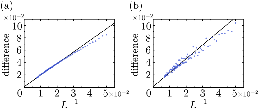
Figure 5: The maximal difference $\max_{E}|\phi(E)-\Phi(E)|$ between the OBC-spectrum-based and Ronkin-function-based Coulomb potentials as a function of the linear size $L$. The adopted Hamiltonian is Eq. (II) [Fig. 2(a)]. The straight line is a linear fitting from data points with $L\geq 55$. (a) The real space is a square of side length $L$, with disorders added on boundary (the same as in Fig. 4(b)). Each data point comes from averaging over six disorder configurations. (b) The real space is a disk of diameter $L$, without disorder (the same as in Fig. 4(c)).

For a Hermitian band, the DOS of OBC system determined by our formulation using the Ronkin function is consistent with the well-known fact that the OBC bulk spectrum and the PBC spectrum are asymptotically identical. This can be proved as follows. Since the eigen-energies belong to the real axis $\mathbb{R}$, one can determine the DOS by Eq. (22), for which knowing $\phi(E)$ for $E\notin\mathbb{R}$ is sufficient. For an arbitrary $E\notin\mathbb{R}$, $\det[E-h(e^{i\bm{k}})]\neq 0$ always holds for all $\bm{k}\in[0,2\pi]^{d}$ because of the Hermiticity of $h(e^{i\bm{k}})$. Thus, $\bm{\mu}=\bm{0}$ does not belong to the amoeba of $\det[E-h(\bm{\beta})]$. In other words, it belongs to one of the amoeba holes. Furthermore, the phase winding number of $\det[E-h(e^{i\bm{k}})]$ along every $k_{j}$-circle is zero. Therefore, the order $\nu_{j}=0$ ($j=1,\cdots d$) at $\bm{\mu}=0$, meaning that $\bm{\mu}=0$ locates in the central hole. It follows that the Ronkin minimum is reached at $\bm{\mu}=0$, i.e., $\phi(E)=R_{\det(E-h)}(\bm{0})$. On the other hand, one can readily see that $R_{\det(E-h)}(\bm{0})$ by definition is the Coulomb potential of the PBC energy spectrum. Therefore, the OBC DOS obtained from Eq. (22) is the same as the PBC DOS in Hermitian cases.

V Amoeba hole closing and spectral boundary

We are now able to prove a powerful theorem about the range of the OBC spectrum in the complex energy plane. It only uses the topology of the amoeba, without having to evaluate the Ronkin function, hence it is convenient in practice.

We denote by $\Lambda$ the set of $E$ where the amoeba of $\det[E-h(\bm{\beta})]$ does not possess a central hole. We will prove the following theorem:

$$\rho(E)=0,\quad E\notin\Lambda.$$ (32)

Thus, at a certain $E$, if the amoeba has a central hole, the DOS is zero at this $E$. In other words, the bulk spectrum is restricted to $\Lambda$.

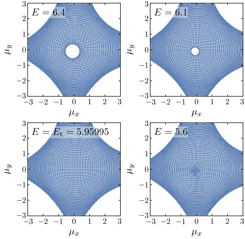
Figure 6: Amoebae for several energies near the band top of the model Eq. (II). As we decrease the energy along the real axis, the central hole of amoeba closes at $E=E_{t}\approx 5.95995$. Parameter values are $t=1$, $t^{\prime}=0.5$, and $\gamma=0.2$, for which the energy spectrum for the square has been shown in Fig. 1(d).

With the results about DOS in the previous section, the proof of this theorem is now simple. When an energy $E_{0}$ is outside $\Lambda$, one must choose $\bm{\mu}$ in the central hole so that Eq. (28) holds. Because the shape of central hole varies continuously as $E$ varies, the central hole should still contain this $\bm{\mu}$ for $E$ sufficiently close to $E_{0}$. Therefore, there exists a neighborhood of $E_{0}$, denoted by $V$, such that for any $E\in V$, the same $\bm{\mu}$ is in the central hole of the amoeba of $\det(E-h)$. Thus, for any $E\in V$, the Ronkin minimum is $\phi(E)=R_{\det(E-h)}(\bm{\mu})$. Recalling the definition of amoeba, we see that $\det[E-h(e^{\bm{\mu}+i\bm{k}})]$ is nowhere zero in $V$ for any $\bm{k}\in T^{d}=[0,2\pi]^{d}$. Furthermore, the Ronkin function can be expressed as $R_{\det(E-h)}(\bm{\mu})=\int_{T^{d}}\left(\frac{dk}{2\pi}\right)^{d}\sum_{i}\log|E-E_{i}(\bm{\beta})|$, in which $\{E_{i}(\bm{\beta})\}$ are the eigenvalues of $h(\bm{\beta})$ ($\bm{\beta}=e^{\bm{\mu}+i\bm{k}}$ as usual). Because $\det(E-h)\neq 0$ implies $|E-E_{i}(\bm{\beta})|\neq 0$, we have $\Delta[\sum_{i}\ln|E-E_{i}(\bm{\beta})|]=0$ and therefore its integration over $T^{d}$ vanishes, leading to $\rho(E)=\Delta\phi(E)/2\pi=0$. This ends our proof of the theorem Eq. (32). Note that this proof only makes use of the original version of Szegö’s theorem, Eq. (24), without invoking the generalized version, Eq. (29).

When $E\in\Lambda$, the DOS is generally nonzero since nothing enforces it otherwise. Thus, the boundary of $\Lambda$, on which the central hole closes, coincides with the boundary of the energy spectrum. In fact, if we assume the validity of the conjecture Eq. (29) and therefore Eq. (19), we have $\rho(E)=\Delta\phi(E)/2\pi$ which is generally nonzero in $\Lambda$. In other words, the support of the DOS is exactly $\Lambda$.

In Fig. 6, we illustrate the amoeba-hole closing for the model Eq. (II). Starting from an energy well above the band top (maximum of the real part of the eigenenergies), we decrease the energy along the real axis. For $E$ larger than a certain energy, the central hole of amoeba exists, though its size shrinks as $E$ decreases. At $E=E_{t}\approx 5.95995$, the central hole closes. According to our proposal, this hole-closing point is identified as the band top. Similarly, the entire spectral boundary can be delineated by hole closing.

In Fig. 7, we compare the results obtained from the amoeba formulation and numerical calculations. We numerically diagonalize the real-space Hamiltonian with increasing sizes and obtain the values of band top, which are then extrapolated to infinite size [Fig. 7 (a)]. The results are strikingly close to the predictions of the amoeba theory [Fig. 7 (a)(b)]. We also do similar comparison for the band bottom (minimum of the real part of the eigenenergies) [Fig. 7 (c)(d)]. Note that the band top and band bottom exhibit different scaling behavior when $L\to\infty$: The finite-size correction $\Delta E_{t}\propto L^{-2}$ for the former [Fig. 7 (a)], and $\Delta E_{b}\propto L^{-1}$ for the latter [Fig. 7 (c)]. It turns out that the former scaling is more accurately obeyed here. Therefore, the error bar of extrapolation is larger for the latter. Despite the larger numerical errors, the numerical results are still in reasonable agreement with the amoeba-theoretic prediction.

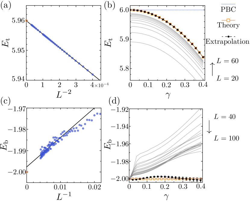
Figure 7: Band top $E_{t}$ and bottom $E_{b}$ obtained from amoeba formulation and numerical calculations. The model is Eq. (II), with $t=1$, $t^{\prime}=0.5$ fixed. In (a)(c), $\gamma$ is fixed to $0.2$. (a) Band top obtained from diagonalizing the real-space Hamiltonian on the disk with diamater $L$. The extrapolation to $L\rightarrow\infty$ agrees well with the amoeba-hole closing point marked as the orange square. (b) Band top as a function of $\gamma$, for increasing $L$ values. The extrapolation to $L\rightarrow\infty$ is shown as black dots, which are in excellent agreement with the amoeba-hole closing points marked as orange squares. The PBC result is shown as the dotted line. (c)(d) The counterparts of (a)(b) for the band bottom. The linear fitting in (c)(d) is based on data from $L\in[80,240]$.

VI Generalized Brillouin zone

In this section, we establish another proposal mentioned at the end of Sec. III, namely that the location of Ronkin minimum represents the GBZ. According to Eq. (32), the DOS can be nonzero only when the central hole of the amoeba of $\det(E-h)$ is absent. Thanks to the convexity of Ronkin function, the minimum location $\bm{\mu}_{\min}$ must be unique in these cases, and therefore the proposal is unambiguous.

The GBZ essentially determines the profiles of the eigenstates of a non-Hermitian lattice Hamiltonian. According to our proposal, an eigenstate with eigen-energy $E$ is expressed asymptotically in the bulk as

$$\psi_{E}(\bm{x})=\sum_{\bm{k}}c_{\bm{k}}\exp\left[\left(i\bm{k}+\bm{\mu}_{\min}\left(E\right)\right)\cdot\bm{x}\right],$$ (33)

where the sum is over all $\bm{k}$ satisfying $\det[E-h(e^{\bm{\mu}_{\text{min}}+i\bm{k}})]=0$, and $c_{\bm{k}}$ are certain $E$-dependent coefficients. Here, $\bm{\mu}_{\min}$ plays the role of the imaginary part of the wave vector, if we define a complex-valued wave vector

$$\tilde{\bm{k}}=\bm{k}-i\bm{\mu}_{\min}.$$ (34)

Equivalently, we can use the variable $\bm{\beta}=e^{i\tilde{\bm{k}}}$ (or $\tilde{\bm{k}}=-i\log\bm{\beta}$), so that $\psi_{E}(\bm{x})=\sum_{\bm{\beta}}c_{\bm{\beta}}\prod_{j=1}^{d}(\beta_{j})^{x_{j}}$. In our theory, the GBZ consists of all points $\bm{\beta}$ subjected to

$$\det[E-h(\bm{\beta})]=0,\quad\log|\bm{\beta}|=\bm{\mu}_{\min}(E).$$ (35)

Note that in our notation the second equation means $\log|\beta_{j}|=(\mu_{\text{min}})_{j}$ ($j=1,2,\cdots,d$). For a $d$-dimensional non-Hermitian system, the GBZ is a $d$-dimensional subspace of the $\bm{\beta}$ space whose real dimension is $2d$. In fact, there are $2d+2$ real unknowns in Eqs. (35), namely the real and imaginary parts of $(\bm{\beta},E)$. Eqs. (35) then impose $d+2$ constraints, meaning that the solution space is $d$-dimensional. Eqs. (35) provide a general approach to calculate the GBZ for higher-dimensional non-Hermitian systems. In practice, we often parameterize the GBZ by $\bm{k}$, treating $\bm{\mu}_{\min}$ as its function. This vectorial function $\bm{\mu}_{\min}(\bm{k})$ is a complete representation of the GBZ. As an application of our theory, the GBZ thus obtained for our model Eq. (II) is shown in Fig. 8(a).

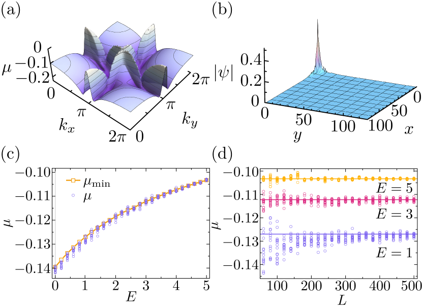
Figure 8: (a) The generalized Brillouin zone of model Eq. (II). Due to the symmetry of interchanging $x$ and $y$ in this model, we have $\mu_{x}=\mu_{y}\equiv\mu_{\text{min}}$ at $\bm{\mu}=\bm{\mu}_{\mathrm{min}}$. We plot $\mu$ as a function of the real part of the wave vector, $\bm{k}=(k_{x},k_{y})$. (b) Typical profile of a bulk eigenstate that exhibits the non-Hermitian skin effect. The eigenstate is taken at $E=-0.003+0.056i$. The system is a square of length $L=130$, with certain random on-site disorders on the boundary. (c)(d) Comparison between $\mu_{\mathrm{min}}$ and the slope $\mu$ of the Green’s function. The latter is defined by extracting $\mu_{x},\mu_{y}$ from $\left\langle\bm{x}\right|(E-H)^{-1}\left|\bm{0}\right\rangle\sim\exp(\mu_{x}x+\mu_{y}y)$, in which $\mu_{x}\approx\mu_{y}$ for our model and therefore we take the average $\mu=(\mu_{x}+\mu_{y})/2$. Here, $H$ is a real-space Hamiltonian defined on a disk with diameter $L$, with random onsite disorder (distributed uniformly in $[-0.5,0.5]$) on the boundary. Each hollow dot represents the result from a disorder configuration. During the fitting of $\mu_{x,y}$, we discard $\bm{x}$’s that are within distance $20$ from the boundary. In (c) we have fixed $L=400$. In (d) we vary $L$ at fixed $E=1,3,5$; the corresponding $\mu_{\text{min}}$’s are shown as horizontal lines.

Now we provide evidences for Eq. (33) and Eqs. (35). First, we show that an eigenstate $|\psi\rangle$ subjected to $H|\psi\rangle=E|\psi\rangle$ shares the same exponential behavior with the Green’s function $G(E)=(E-H)^{-1}$. To see this, we decompose the OBC Hamiltonian into its eigenstates:

$$H=\sum_{n}\epsilon_{n}\left|nR\right\rangle\left\langle nL\right|,$$ (36)

where the sum is over all eigenstates. $\left|nR\right\rangle$ and $\left\langle nL\right|$ are the right and left eigenstates, respectively, which satisfy

$$H\left|nR\right\rangle=\epsilon_{n}\left|nR\right\rangle,\quad\left\langle nL\right|H=\epsilon_{n}\left\langle nL\right|.$$ (37)

They are orthonormalized as $\langle mL|nR\rangle=\delta_{mn}$. Suppose that $\bm{x}$ and $\bm{0}$ are real-space locations far from the boundary. The Green’s function is related to the eigenstates in the following way:

$$\phantom{=}\partial_{\bar{E}}\left\langle\bm{x}\right|\left(E-H\right)^{-1}\left|\bm{0}\right\rangle$$

$$=\sum_{n}\langle\bm{x}|nR\rangle\langle nL|\bm{0}\rangle\partial_{\bar{E}}\dfrac{1}{E-\epsilon_{n}}$$

$$=\pi\sum_{n}\langle\bm{x}|nR\rangle\langle nL|\bm{0}\rangle\delta(E-\epsilon_{n})$$

$$=\sum_{\epsilon_{n}=E}K_{n}\langle\bm{x}|nR\rangle,$$ (38)

where $\bar{E}$ is the complex conjugate of $E$, and $K_{n}$ are constants. We have used the formula $\partial_{\bar{z}}z^{-1}=\pi\delta(z)$. We emphasize that $E$ is taken in the OBC energy spectrum, otherwise the $\delta$ function in Eq. (VI) would vanish. The right-hand side of Eq. (VI) is a linear combination of all eigenstates with energy $E$. Thus, these eigenstates share the same exponential behavior with $\partial_{\bar{E}}\left\langle\bm{x}\right|\left(E-H\right)^{-1}\left|\bm{0}\right\rangle$ and therefore the Green’s function $\left\langle\bm{x}\right|\left(E-H\right)^{-1}\left|\bm{0}\right\rangle$ itself. Suppose that the behavior is $\left\langle\bm{x}\right|\left(E-H\right)^{-1}\left|\bm{0}\right\rangle\sim\exp(\sum_{j=1}^{d}\mu_{j}x_{j})$. To validate Eq. (33) and Eqs. (35), we should verify that $\mu_{j}=(\mu_{\text{min}})_{j}$. We have numerically confirmed this relation [Fig. 8(c)(d)]. Note that in principle one may also able to validate Eq. (33) and Eqs. (35) by the exponential behavior of eigenstates themselves. However, the Green’s function approach is computationally less expensive, which allows us to compute for relatively large $L$ within reasonable time.

VII Non-Bloch band topology

It has been found recently that the topological numbers defined on the conventional Brillouin zone fail to characterize the topological edge states and bulk-boundary correspondence in non-Hermitian systems. To correctly account for the topological edge modes, the non-Bloch topological invariants defined on the GBZ have been proposed. In practice, most of their applications are restricted to 1D, because a general calculable formulation of GBZ in higher dimension has been lacking. Based on the amoeba formulation, we are now able to address the non-Bloch band topology in higher dimensions. Specifically, the non-Bloch Chern number, which was previously calculated only by continuum approximation, can now be calculated in the entire GBZ as is.

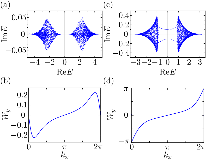
Figure 9: Energy spectrum and band topology of the non-Hermitian Chern-band model Eq. (VII). (a) Energy spectrum by diagonalizing the real-space Hamiltonian on a square of side length $L=60$, with random onsite disorders on boundary. Parameters are taken in the topologically trivial regime: $m=2.6$, $\gamma=0.4$. (b) The Berry phase $W_{y}$ along a circle in the $k_{y}$ direction ($k_{x}=\mathrm{const}$). The non-Bloch Chern number $C=[W_{y}(2\pi)-W_{y}(0)]/2\pi=0$. (c) Energy spectrum by diagonalization, calculated under the same setting as in (a). Parameters are taken in the topologically non-trivial regime: $m=1.2$, $\gamma=0.4$. Topological edge states are observed. (d) The Berry phase as a function of $k_{x}$, with $W_{y}(2\pi)-W_{y}(0)=2\pi$ and therefore $C=1$.

To be concrete, we consider the following non-Hermitian Chern-band model Yao et al. (2018)

$$h\left(e^{i\bm{k}}\right) =\left(v\sin k_{x}+i\gamma\right)\sigma_{x}+\left(v\sin k_{y}+i\gamma\right)\sigma_{y}$$

$$\phantom{=}+\left(m-t\cos k_{x}-t\cos k_{y}\right)\sigma_{z}.$$ (39)

The real-space Hamiltonian reads

$$H =\sum_{\bm{x}}\sum_{j=x,y}\left|\bm{x}\right\rangle\left(-\dfrac{i}{2}v\sigma_{j}-\dfrac{1}{2}t\sigma_{z}\right)\left\langle\bm{x}+\bm{e}_{j}\right|+\mathrm{H.c.}$$

$$\phantom{=}+\sum_{\bm{x}}\left|\bm{x}\right\rangle\left(m\sigma_{z}+i\gamma\sigma_{x}+i\gamma\sigma_{y}\right)\left\langle\bm{x}\right|,$$ (40)

where $\bm{x}$ are 2D integer coordinates, and $\bm{e}_{j}$ is the unit vector in the $j$-th direction [see Fig. 2(b)]. We set $t=v=1$ for simplicity.

This model is known to have a Chern insulator phase as well as a trivial insulator phase in the Hermitian limit ($\gamma=0$) X.L. Qi et al. (2006). It has Chern number $C=1$ when $0<m<2$; $C=-1$ when $-2<m<0$; and $C=0$ otherwise. We shall focus on the phase boundary between $C=0$ and $C=1$ . When we turn on the non-Hermitian term ($\gamma\neq 0$), the phase boundary extends into a curve in the $m$-$\gamma$ plane, which should be predicted by the non-Bloch band theory. In particular, the number of chiral edge modes in each phase is given by the non-Bloch Chern number evaluated on the GBZ, which is a two-dimensional subspace of the four-dimensional $\bm{\beta}$ space. Alternatively, we may take $\tilde{\bm{k}}=\bm{k}-i\bm{\mu}=\log\bm{\beta}$ as the coordinate system, in which the GBZ is two-dimensional because $\bm{\mu}$ is treated as a function of $\bm{k}$, so that the GBZ can be parametrized by $\bm{k}$. Thus, the non-Bloch Chern number can be viewed as the conventional Chern number of $h(e^{i\tilde{\bm{k}}})$, with $\tilde{\bm{k}}\in\text{GBZ}$. For a band labelled by $\alpha$, the non-Bloch Chern number reads

$$C=\dfrac{1}{2\pi i}\int_{T^{2}}dk_{x}dk_{y}\,\epsilon^{ij}\partial_{i}\langle\tilde{\bm{k}},\alpha,L|\partial_{j}|\tilde{\bm{k}},\alpha,R\rangle,$$ (41)

where $\epsilon^{xy}=-\epsilon^{yx}=1$, $\partial_{j}$ refers to $\frac{\partial}{\partial k_{j}}$, $\langle\tilde{\bm{k}},\alpha,L|$ and $|\tilde{\bm{k}},\alpha,R\rangle$ is the left and right eigenstates of the $\alpha$ band, respectively. We shall focus on the “valence band” ($\operatorname{Re}E<0$), labelled as $\alpha=-$.

More intuitively, the non-Bloch Chern number can be expressed as the change of Berry phase along circular sections of the GBZ in the $y$-direction, i.e., $C=\frac{1}{2\pi}\int_{0}^{2\pi}\frac{dW_{y}(k_{x})}{dk_{x}}dk_{x}=[W_{y}(2\pi)-W_{y}(0)]/2\pi$, in which the Berry phase

$$W_{y}\left(k_{x}\right) =-i\int_{0}^{2\pi}\left\langle\tilde{\bm{k}},-,L\right|\partial_{k_{y}}\left|\tilde{\bm{k}},-,R\right\rangle dk_{y}$$

$$=-\int_{0}^{2\pi}\dfrac{h_{x}\partial_{k_{y}}h_{y}-h_{y}\partial_{k_{y}}h_{x}}{2|h|\left(|h|+h_{z}\right)}dk_{y},$$ (42)

where we have written the Bloch Hamiltonian as $h=h_{x}\sigma_{x}+h_{y}\sigma_{y}+h_{z}\sigma_{z}$, and $|h|=\sqrt{h_{x}^{2}+h_{y}^{2}+h_{z}^{2}}$. Here, $h_{x,y,z}$ can be readily read from Eq. (VII) by the substitution $\bm{k}\rightarrow\tilde{\bm{k}}$: $h_{x}=v\sin\tilde{k}_{x}+i\gamma$, $h_{y}=v\sin\tilde{k}_{y}+i\gamma$, and $h_{z}=m-t\cos\tilde{k}_{x}-t\cos\tilde{k}_{y}$.

In Fig. 9, we show the energy spectrum and non-Bloch Chern number for the Chern-band model. As an example, we fix $\gamma=0.4$, and take $m=2.6$ and $m=1.2$. From Fig. 9(c)(d), we read for each case that $C=0$ and $C=1$, respectively. In Fig. 9(b), topological edge states are indeed seen, being consistent with the nonzero non-Bloch topological invariant $C=1$.

Table 1: Topological phase boundary $m_{c}$ as a function of $\gamma$. The decay factor $\mu$ (equal in both $x$- and $y$-direction) at $E=0$ and “$m_{c}$ amoeba” are determined using the amoeba method, with numerical error $<$ $1\times 10^{-6}$. “$m_{c}$ numerical” is adopted from Ref. Yao et al. (2018), which is obtained by numerical diagonalization of real-space Hamiltonian with numerical error $<$ $3\times 10^{-4}$.

$\gamma$	$\mu$	$m_{c}$ amoeba	$m_{c}$ numerical
$0.00$	$0.000000$	$2.000000$	$2.0000$
$0.05$	$0.049979$	$2.002498$	$2.0025$
$0.10$	$0.099834$	$2.009975$	$2.0100$
$0.15$	$0.149443$	$2.022375$	$2.0225$
$0.20$	$0.198690$	$2.039608$	$2.0400$
$0.25$	$0.247466$	$2.061553$	$2.0625$
$0.30$	$0.295673$	$2.088061$	$2.0885$
$0.35$	$0.343222$	$2.118962$	$2.1200$
$0.40$	$0.390035$	$2.154066$	$2.1540$
$0.45$	$0.436050$	$2.193171$	$2.1940$
$0.50$	$0.481212$	$2.236068$	$2.2360$

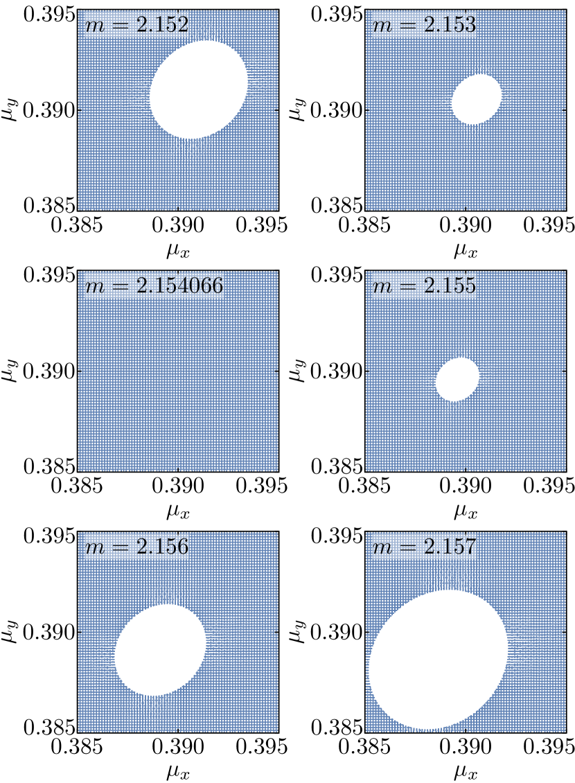
Figure 10: The amoeba-based procedure of locating the phase boundary in Table 1. The figures show the amoebae, zooming in on the central hole, with $\gamma=0.4$ fixed and $m$ varied. The central hole closes at exactly one point $m=m_{c}\approx 2.154066$, which is where the topological phase transition occurs.

For the present model, the precise phase boundary can even be analytically determined by the amoeba formulation. In the $m$-$\gamma$ plane, the phase boundary between the $C=0$ and $C=1$ phases is a curve, which can be viewed as a function $m_{c}(\gamma)$, i.e., the phase transition point is $m_{c}(\gamma)$ for a fixed $\gamma$. On the phase boundary, the energy gap about $E=0$ closes, and $E=0$ belongs to the energy spectrum. Thus, we can find $m_{c}$ by inspecting when the central hole of the amoeba at $E=0$ closes. The exact formula for $m_{c}$ is found to be

$$m_{c}=2\sqrt{1+\gamma^{2}}.$$ (43)

Perturbative result of this formula was obtained in Ref. Yao et al. (2018), and recently a result to the sixth order of $\gamma$ was reported in Ref. Takane (2021). Our derivation of Eq. (43) is as follows. We focus on the special solution of the characteristic equation that satisfies $\beta_{x}=\beta_{y}\equiv\beta$, as the symmetry of the model allows. The characteristic equation $\det[E-h(\beta_{x},\beta_{y})]=0$ becomes

$$\left(m-\beta-\beta^{-1}\right)^{2}-2\left(\gamma-\dfrac{\beta-\beta^{-1}}{2}\right)^{2}=0.$$ (44)

In a neighborhood of the phase transition, we numerically notice that the four roots of the above quartic equation are all real, and that the second-largest and third-largest (the middle two) roots, under the logarithm, are on the boundary of the central hole of the amoeba. Hence requiring the central hole to vanish is equivalent to requiring the middle two roots to be equal. Solving this requirement leads to the final result Eq. (43).

Eq. (43) is verified up to high precision by numerically locating where the central hole vanishes, as listed in Table 1. From the amoeba-based approach, Fig. 10 illustrates locating the critical value $m_{c}$ for the case $\gamma=0.4$. In practice, it is convenient to search $m_{c}(\gamma)$ by iteration: plot the amoeba at a consecutive sequence of $m$’s, find the interval with the smallest central-hole area, then zoom in on the central hole and plot amoebae again. On the other hand, $m_{c}$ can also be determined by numerically diagonalizing the real-space Hamiltonian and finding where the band gap closes Yao et al. (2018). We compare the amoeba-based and numerical-diagonalization results, which agree well with each other.

In the amoeba formulation, an exact expression for the decay factor $\mu_{x}=\mu_{y}\equiv\mu$ at the band-closing point $E=0$ can also be obtained:

$$\mu=\log(\sqrt{\gamma^{2}+1}+\gamma).$$ (45)

This result is very close to the $\mu$ values listed in Table 1, which are numerically obtained by locating the amoeba-hole closing points. We remarks that a first-order approximation $\mu=\gamma+o(\gamma)$ was found in Ref. Yao et al. (2018).

VIII Spectral inequality

As one of the applications of the amoeba formulation, we shall prove a general inequality about spectral radius. For a matrix or operator $H$, the spectral radius $\rho(H)$ is defined to be the largest absolute value of the eigenvalues. Our spectral inequality states that for a non-Hermitian lattice Hamiltonian with translational symmetry in the bulk, the PBC spectral radius is always larger or equal to its OBC counterpart:

$$\rho(H_{\text{OBC}})\leq\rho(H_{\text{PBC}}).$$ (46)

Note that we are interested in the thermodynamic limit in which all edge-state contribution vanishes. It is evident that Figs. 1(a) and (d) satisfy the inequality.

To begin, a simple fact about the electrostatic potential is useful. Suppose that a Coulomb potential $\Phi$ is generated by a DOS (charge) distribution $\rho$ in the 2D complex plane, i.e., $\Phi(E)=\int d^{2}E^{\prime}\,\log|E-E^{\prime}|\rho(E^{\prime})$. We are interested in the average potential on a circle, say $|E|=R$, which reads $\bar{\Phi}=\frac{1}{2\pi}\int_{0}^{2\pi}d\theta\,\log|Re^{i\theta}-E^{\prime}|\rho(E^{\prime})$. To calculate this average, one just need to treat all charges inside the circle as distributed uniformly on the circle, and all charges outside as they are. For example, the contribution of a point charge $q$ with radial coordinate $r<R$ is $\bar{\Phi}=q\log R$, while that of point charge with $r>R$ is $\bar{\Phi}=q\log r$. This can be readily proved by using the Jensen’s formula Eq. (14). Taking $g(Re^{i\theta})=Re^{i\theta}-re^{i\alpha}$ in Eq. (14), the left-hand side of the equation is the average potential generated by a point charge at $E^{\prime}=re^{i\alpha}$, and Eq. (14) becomes

$$\bar{\Phi}=\left\{\begin{aligned} &\log R,\quad&r<R,&\\ &\log r,\quad&r>R.\end{aligned}\right.$$ (47)

Now we proceed with the spectral radius inequality. From Sec. IV, we know that the Coulomb potential generated by the OBC DOS is equal to the minimum of the Ronkin function, $\Phi_{\text{OBC}}(E)=\min_{\bm{\mu}}R_{\det(E-h)}(\bm{\mu})$. On the other hand, we can also write the Coulomb potential generated by the PBC DOS in terms of the Ronkin function at $\bm{\mu}=0$:

$$\Phi_{\mathrm{PBC}}(E)=R_{\det(E-h)}(\bm{0}).$$ (48)

Hence

$$\Phi_{\mathrm{OBC}}(E)\leq\Phi_{\mathrm{PBC}}(E).$$ (49)

It follows that the average satisfies

$$\bar{\Phi}_{\mathrm{OBC}}\leq\bar{\Phi}_{\mathrm{PBC}}.$$ (50)

Taking a circle $|E|=R$ that surrounds the whole PBC spectrum, then the average potential on this circle is $\bar{\Phi}_{\mathrm{PBC}}=Q\log R$, where $Q$ is the total charge, which is equal to the number of bands of the specific lattice model. Since the total charge of the OBC DOS is also $Q$, the aforementioned electrostatic fact implies that $\bar{\Phi}_{\mathrm{OBC}}\geq Q\log R$, with “$=$” reached when the charge density vanishes outside the circle. Combining this with Eq. (50), we obtain the identity $\bar{\Phi}_{\mathrm{OBC}}=Q\log R$. Consequently, the OBC DOS is zero outside the circle, which means that the OBC spectral radius is no larger than the PBC counterpart.

An alternative proof of the spectral inequality is based on Eq. (32). We denote the PBC spectral (outer) boundary as $S$, which consists of one or several closed curves (note that the spectrum may also have inner boundary, which is not included in $S$. For example, an annulus-like spectrum has an outer and an inner boundary). Consider an energy $E$ outside $S$. Since $E$ is not in the PBC spectrum, $\bm{\mu}=0$ must belong to the complement of the amoeba of $\det(E-h)$. Furthermore, one can see that $\bm{\mu}=0$ locates in the central hole. In fact, in the $|E|\rightarrow\infty$ limit (with $\bm{\mu}=0$ fixed), the phase of $\det[E-h(\bm{\beta})]$ is determined solely by $E$ and independent of $\bm{k}$, and therefore the phase winding number along each $k_{j}$-circle is zero [cf. Eq. (11) and Eq. (12)]. It follows that, for sufficiently large $|E|$, the order $\bm{\nu}=0$ at $\bm{\mu}=0$, i.e., $\bm{\mu}=0$ locates in the central hole. For any $E$ outside $S$, one may connect $E$ to infinity by a path that does not intersect $S$. Since $\bm{\mu}=0$ is always in the same amoeba hole as $E$ varies along this path, this amoeba hole must be the central hole. Thus, for any $E$ outside $S$, $\bm{\mu}=0$ locates in the central hole of amoeba. It follows from Eq. (32) that the OBC DOS $\rho_{\text{OBC}}(E)=0$ outside $S$. Therefore, the OBC spectrum is enclosed by the PBC spectral boundary. This result is slightly stronger than (and clearly implies) the spectral inequality Eq. (46).

A corollary is immediately implied: The spectral range of the real (or imaginary) part of the OBC spectrum is within its PBC counterpart, i.e., one has the following general inequalities:

$$\max\operatorname{Re}(\epsilon_{n,\text{OBC}}) \leq \max\operatorname{Re}(\epsilon_{n,\text{PBC}}),$$ (51)

$$\max\operatorname{Im}(\epsilon_{n,\text{OBC}}) \leq \max\operatorname{Im}(\epsilon_{n,\text{PBC}}),$$ (52)

$$\min\operatorname{Re}(\epsilon_{n,\text{OBC}}) \geq \min\operatorname{Re}(\epsilon_{n,\text{PBC}}),$$ (53)

$$\min\operatorname{Im}(\epsilon_{n,\text{OBC}}) \geq \min\operatorname{Im}(\epsilon_{n,\text{PBC}}).$$ (54)

In view of the significance of energy spectrum, the spectral inequalities have various implications, some of which have already been exploited. In one dimension, one of the spectral inequality, Eq. (52), has played important roles for the directional amplification McDonald et al. (2018); Xue et al. (2021); Wanjura et al. (2020). In the context of open quantum systems, the spectral inequalities are closely related to the boundary sensitivity of Liouvillian gap and relaxation time Song et al. (2019b); Haga et al. (2021); Yang et al. (2022). Our general statement and proof of the spectral inequalities pave a groundwork for their higher-dimensional applications.

IX Concluding remarks

In this work, we have formulated an amoeba theory of the non-Hermitian skin effect and non-Bloch band theory in arbitrary spatial dimensions. It provides a theoretical framework for studying periodic non-Hermitian systems without the serious dimensional limitation. Among other applications, our theory offers a general yet efficient approach to compute the key physical quantities of non-Hermitian systems, such as the energy spectrum, density of states, and generalized Brillouin zone.

Although the initial version of non-Bloch band theory was formulated under the open-boundary condition (OBC), the GBZ concept in 1D is also generalizable to other boundary conditions such as the domain wall cases Deng and Yi (2019). Nevertheless, it seems that the amoeba approach, as we now understand, naturally corresponds to the standard OBC systems. Thus, we have focused on the OBC cases throughout the present paper. Compared to other boundary conditions, OBC is especially important in many senses. First, the OBC is experimentally the most relevant because realistic systems often have OBC. Second, taking OBC enables investigation of both bulk and boundary physics, while other boundary conditions including PBC is blind to boundary phenomena. Third, even certain measurable physical quantities far from the boundary can be naturally expressed in terms of the GBZ of OBC rather than the conventional BZ associated with PBC Longhi (2019, 2019), though it is in principle free to choose the boundary condition when investigating the physics deep in the bulk. In this sense, the OBC seems to be an advantageous choice even for studying certain bulk physics.

We would also like to remark that not all aspects of this work are mathematically rigorous. Although numerical evidences are supplied to support the results whenever a mathematically strict derivation is unavailable, a fully rigorous proof of all our main results is of course desirable.

In view of the ubiquitous existence of periodic structures in both natural and synthetic systems, it is hoped that our theory can find wide applications in the abundant non-Hermitian phenomena. For example, our formulation can be naturally applied to open quantum systems in the free-particle limit, for which the energy spectrum of the non-Hermitian Liouvillian superoperator determines the dynamics and relaxation Song et al. (2019b); Haga et al. (2021). Our theory immediately enables calculating the relevant quantities beyond 1D. Furthermore, for many-body non-Hermitian systems, our amoeba theory may still be a good starting point for including the interaction effects, which will be left for future work.

*

Appendix A A brief proof of the Szegö’s limit theorem

In this Appendix we provide a sketch of proof for the Szegö’s limit theorem Eq. (24), along with an estimation of the inverse of a Toeplitz matrix. We derive concrete conditions for the theorems to hold and explain their intuitions. A thorough proof of the Szegö’s limit theorem and related techniques have been established in mathematical literatures Widom (1974b, 1980); Doktorskii (1984). But for the readers’ convenience, we sketch and rephrase them in physicist-oriented languages.

Let us consider a subspace $\Omega$ of the $d$-dimensional Euclidean space. The number of unit cells in $\Omega$ is then $O(L^{d})$, and the number of unit cells on the boundary is $O(L^{d-1})$, where $L$ is the linear scale of $\Omega$ (e.g., the side length of a square, or the diameter of a disk).

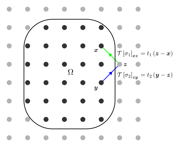
Figure 11: Illustration of Eq. (57). The matrix element of $\mathcal{T}\left[\sigma_{1}\sigma_{2}\right]-\mathcal{T}\left[\sigma_{1}\right]\mathcal{T}\left[\sigma_{2}\right]$ is nonzero only in a neighborhood of the boundary of $\Omega$.

Consider two Toeplitz matrices $\mathcal{T}[\sigma_{1}]$ and $\mathcal{T}[\sigma_{2}]$ defined in $\Omega$. Both of them are $N\times N$ matrices, where $N$ is the number of unit cells (labelled by integer-valued coordinates) in $\Omega$. We first establish the following relation:

$$\left\|\mathcal{T}\left[\sigma_{1}\sigma_{2}\right]-\mathcal{T}\left[\sigma_{1}\right]\mathcal{T}\left[\sigma_{2}\right]\right\|_{1}=O\left(L^{d-1}\right),$$ (55)

where we have used the Schatten norm for operators: $\left\|T\right\|_{p}$ is the $p$-norm of all singular values $\left\{s_{n}\right\}$ of $T$:

$$\left\|T\right\|_{p}=\left(\sum_{n}s_{n}^{p}\right)^{1/p}.$$ (56)

For this kind of relation, we use the notation $\mathcal{T}[\sigma_{1}\sigma_{2}]\approx\mathcal{T}[\sigma_{1}]\mathcal{T}[\sigma_{2}]$. The $(\bm{x},\bm{y})$ matrix element of $\mathcal{T}[\sigma_{1}\sigma_{2}]-\mathcal{T}[\sigma_{1}]\mathcal{T}[\sigma_{2}]$ reads

$$\sum_{\bm{z}\notin\Omega}t_{1}\left(\bm{z}-\bm{x}\right)t_{2}\left(\bm{y}-\bm{z}\right),$$ (57)

where $\bm{x}$, $\bm{y}$ and $\bm{z}$ are integer coordinates; $t_{1,2}$ are the hopping coefficients that appear in $\mathcal{T}[\sigma_{1,2}]$:

$$t_{1,2}(\bm{n})=\int_{T^{d}}\left(\dfrac{d\theta}{2\pi}\right)^{d}\sigma_{1,2}(e^{i\bm{\theta}})e^{-i\bm{n}\cdot\bm{\theta}}.$$ (58)

Note that in Eq. (57) $\bm{x},\bm{y}\in\Omega$ while $\bm{z}\in\Omega^{c}$, where $\Omega^{c}=\mathbb{Z}^{d}\backslash\Omega$. The terms $\sum_{\bm{z}\in\Omega}t_{1}(\bm{z}-\bm{x})t_{2}(\bm{y}-\bm{z})$ appear in both $\mathcal{T}[\sigma_{1}\sigma_{2}]$ and $\mathcal{T}[\sigma_{1}]\mathcal{T}[\sigma_{2}]$ and therefore do not contribute to their difference.

It is clear that each term in Eq. (57) can be nonzero only when both $\bm{x}$ and $\bm{y}$ are near the boundary (see also Fig. 11). Thus, it is intuitive that the matrix norm of $\mathcal{T}[\sigma_{1}\sigma_{2}]-\mathcal{T}[\sigma_{1}]\mathcal{T}[\sigma_{2}]$ is of order $O(L^{d-1})$. A more formal proof is based on the Hölder’s inequality for matrix norms, which states that $\left\|AB\right\|_{1}\leq\left\|A\right\|_{p}\left\|B\right\|_{q}$ holds for all $p\in[1,\infty]$ and $q$ satisfying $1/p+1/q=1$. Defining $\left(T_{1}\right)_{\bm{x},\bm{z}}=t_{1}(\bm{z}-\bm{x})$ that maps $\Omega^{c}$ to $\Omega$ and $\left(T_{2}\right)_{\bm{z},\bm{y}}=t_{2}(\bm{y}-\bm{z})$ that maps $\Omega$ to $\Omega^{c}$, we see that Eq. (57) becomes $(T_{1}T_{2})_{\bm{x},\bm{y}}$. According to Hölder’s inequality, we have

$$\left\|T_{1}T_{2}\right\|_{1}\leq\left\|T_{1}\right\|_{2}\left\|T_{2}\right\|_{2},$$ (59)

and we are only left with showing $\left\|T_{j}\right\|_{2}^{2}=O(L^{d-1})$ for $j=1,2$. Recalling that the singular values of $T_{1}$ are the eigenvalues of $\sqrt{T_{1}T_{1}^{\dagger}}$, $\left\|T_{1}\right\|_{2}^{2}$ by definition equals the trace of $T_{1}T_{1}^{\dagger}$, whose elements read

$$\left(T_{1}T_{1}^{\dagger}\right)_{\bm{x},\bm{x^{\prime}}}=\sum_{\bm{z}\in\Omega^{c}}t_{1}(\bm{z}-\bm{x})t_{1}^{\dagger}(\bm{z}-\bm{x^{\prime}}).$$ (60)

Hence

$$\left\|T_{1}\right\|_{2}^{2} =\operatorname{tr}T_{1}T_{1}^{\dagger}$$

$$=\sum_{\bm{x}\in\Omega,\bm{z}\in\Omega^{c}}\operatorname{tr}t_{1}(\bm{z}-\bm{x})t_{1}^{\dagger}(\bm{z}-\bm{x})$$

$$=\sum_{\bm{x}\in\Omega,\bm{z}\in\Omega^{c}}\left\|t_{1}(\bm{z}-\bm{x})\right\|_{2}^{2}$$

$$=\sum_{\bm{u}}\left\|t_{1}(\bm{u})\right\|_{2}^{2}\operatorname{vol}\left((\Omega+\bm{u})\cap\Omega^{c}\right).$$ (61)

In the last line we have substituted $\bm{z}-\bm{x}$ by $\bm{u}$. The volume accounts for the multiplicity of the term $\left\|t_{1}(\bm{u})\right\|_{2}^{2}$, which is the number of lattice points in the overlap of $\Omega$ translated by $\bm{u}$ and the complement $\Omega^{c}$. It is roughly $|\bm{u}|$ times the surface area of $\Omega$, denoted by $|\partial\Omega|$. For short-ranged Toeplitz matrices, we have $t_{j}(\bm{u})=0$ when $|\bm{u}|$ is beyond the hopping range. Therefore, only a boundary layer contributes to the summation over $|\bm{u}$, which means

$$\left\|T_{1}\right\|_{2}^{2}=O\left(L^{d-1}\right).$$ (62)

A similar estimation holds for $T_{2}$. These two estimates together prove Eq. (55).

A caveat arises when either $\mathcal{T}\left[\sigma_{1}\right]$ or $\mathcal{T}\left[\sigma_{2}\right]$ is not short-ranged, meaning e.g., $t_{1}(\bm{u})$ is nonzero even for large $|\bm{u}|$. For a large system size, Eq. (A) is lesser than

$$\sum_{\bm{u}}\left\|t_{1}(\bm{u})\right\|_{2}^{2}\left|\bm{u}\right|\left|\partial\Omega\right|.$$ (63)

Thus, a necessary condition for Eq. (55) and all the following theorems to hold is that

$$\sum_{\bm{u}}\left|\bm{u}\right|\left\|t(\bm{u})\right\|_{2}^{2}<\infty$$ (64)

is satisfied for all Toeplitz matrices concerned. This tells us that our theorems also hold for certain long-ranged Hamiltonians, as long as the hopping decays sufficiently fast at long distance.

Now let $\sigma_{1}=\sigma$, $\sigma_{2}=\sigma^{-1}$ and assume that $\sigma$ is invertible, we have

$$\left\|I-\mathcal{T}\left[\sigma\right]\mathcal{T}\left[\sigma^{-1}\right]\right\|_{1}=O\left(L^{d-1}\right),$$ (65)

where $I$ is the identity matrix. Intuitively, multiplying $\mathcal{T}[\sigma]^{-1}$ on the left, we would expect the following asymptotic inversion formula

$$\left\|\mathcal{T}\left[\sigma\right]^{-1}-\mathcal{T}\left[\sigma^{-1}\right]\right\|_{1}=O\left(L^{d-1}\right).$$ (66)

Nevertheless, this multiplication should not be done without discretion. To be precise, we shall use Hölder’s inequality again

$$\left\|\mathcal{T}\left[\sigma\right]^{-1}-\mathcal{T}\left[\sigma^{-1}\right]\right\|_{1}$$

$$\leq\left\|\mathcal{T}[\sigma]^{-1}\right\|_{\infty}\left\|I-\mathcal{T}\left[\sigma\right]\mathcal{T}\left[\sigma^{-1}\right]\right\|_{1}.$$ (67)

Therefore, a condition for Eq. (66) is that $\left\|\mathcal{T}[\sigma]^{-1}\right\|_{\infty}$, which is the largest of its singular values, is finite. Further, this is tantamount to asking if $\mathcal{T}[\sigma]$ itself has a null singular value. Since most of its singular values form bulk bands and have a finite gap from zero, the zeros should be of certain topological origin. They are intimately related to the index theorem, or to say the bulk-boundary correspondence in free systems. If the symbol has a nontrivial topological index, then the corresponding Toeplitz matrix have either nonempty kernel or nonempty cokernel. Either case implies that $\mathcal{T}[\sigma]\mathcal{T}[\sigma]^{\dagger}$ is not fully ranked and has a zero eigenvalue. As to 1D Toeplitz matrices, the topological index is well-known to be the negative of the winding number of $\det\sigma(e^{i\theta})$ Douglas (1998). To ensure the Toeplitz matrix does not have null singular values, we impose a homotopy condition that the symbol $\sigma(e^{i\bm{\theta}})$ is homotopic to a constant symbol $\sigma_{\text{const}}(e^{i\bm{\theta}})=1$ . This requirement may be too strong for now, but we shall see in a moment that it arises again when defining the matrix logarithm.

The asymptotic inversion formula Eq. (66) aims at finding a good surrogate for the inverse of $\mathcal{T}[\sigma]$ in the bulk, $\mathcal{T}[\sigma^{-1}]$, which is calculable by mere integration. We remark that Widom also proposed an explicit expression for the subleading term in $\mathcal{T}[\sigma]^{-1}=\mathcal{T}[\sigma^{-1}]+O(L^{d-1})+o(L^{d-1})$ in the continuous case, which is unneeded in the present paper so is omitted. The Szego’s limit theorem also naturally inherits an expression for the subleading term $O(L^{d-1})$.

Next, we move on to the Szegö’s limit theorem Eq. (24). Since $\log\det A=\operatorname{tr}\log A$, it is equivalent to the following trace formula:

$$\operatorname{tr}\log\left(\mathcal{T}\left[\sigma\right]\right)=N\int_{T^{d}}\left(\dfrac{d\theta}{2\pi}\right)^{d}\operatorname{tr}\log\left(\sigma\left(e^{i\bm{\theta}}\right)\right)+O\left(L^{d-1}\right),$$ (68)

where $N$ is the number of lattice points in $\Omega$. The reason why we focused on the $1$-norm becomes clear now, since $\operatorname{tr}A\leq\left\|A\right\|_{1}$ for any matrix or operator $A$. In order to properly define a logarithm for the symbol, we must rely on the homotopy path imposed earlier. Let $\sigma_{\lambda}(e^{i\bm{\theta}})$ be one of these paths, which is a function from $\lambda\in[0,1]$ to the space of symbols. For example, we show a possible construction of such homotopy path in the context of taking $\sigma(e^{i\bm{\theta}})=E-h(e^{\bm{\mu}+i\bm{\theta}})$. If we can find a continuous path of $E_{\lambda}$ from $E_{0}=E$ to $E_{1}=\infty$ that avoids the spectral range of $h(e^{\bm{\mu}+i\bm{\theta}})$, then the path of symbols is

$$\sigma_{\lambda}(e^{i\bm{\theta}})=\frac{E_{\lambda}-h(e^{\bm{\mu}+i\bm{\theta}})}{E_{\lambda}-E+1}.$$ (69)

A consequence of null homotopy is that the winding number of $\sigma$ along any circle on $T^{d}$ is identically zero.

The logarithm in the Szegö’s limit theorem is thus defined as

$$\log\sigma=\int_{0}^{1}\sigma_{\lambda}^{\prime}\sigma_{\lambda}^{-1}\,d\lambda,$$ (70)

$$\log\mathcal{T}\left[\sigma\right]=\int_{0}^{1}\mathcal{T}\left[\sigma_{\lambda}^{\prime}\right]\mathcal{T}\left[\sigma_{\lambda}\right]^{-1}\,d\lambda,$$ (71)

where a prime denotes derivative with respect to $\lambda$. Using Eq. (66) we deduce

$$\log\mathcal{T}\left[\sigma\right] \approx\int_{0}^{1}\mathcal{T}\left[\sigma_{\lambda}^{\prime}\right]\mathcal{T}\left[\sigma_{\lambda}^{-1}\right]\,d\lambda$$

$$\approx\int_{0}^{1}\mathcal{T}\left[\sigma_{\lambda}^{\prime}\sigma_{\lambda}^{-1}\right]\,d\lambda$$

$$=\mathcal{T}\left[\log\sigma\right].$$ (72)

Taking trace on both sides, the Szegö’s limit theorem is proved.

References

- Ashida et al. (2020) Yuto Ashida, Zongping Gong, and Masahito Ueda, “Non-hermitian physics,” Advances in Physics 69, 249–435 (2020).
- Bergholtz et al. (2021) Emil J. Bergholtz, Jan Carl Budich, and Flore K. Kunst, “Exceptional topology of non-hermitian systems,” Rev. Mod. Phys. 93, 015005 (2021).
- Ding et al. (2022) Kun Ding, Chen Fang, and Guancong Ma, “Non-Hermitian topology and exceptional-point geometries,” Nature Reviews Physics 4, 745–760 (2022), arXiv:2204.11601 [quant-ph] .
- Yao and Wang (2018) Shunyu Yao and Zhong Wang, “Edge states and topological invariants of non-hermitian systems,” Phys. Rev. Lett. 121, 086803 (2018).
- Kunst et al. (2018) Flore K. Kunst, Elisabet Edvardsson, Jan Carl Budich, and Emil J. Bergholtz, “Biorthogonal bulk-boundary correspondence in non-hermitian systems,” Phys. Rev. Lett. 121, 026808 (2018).
- Lee and Thomale (2019) Ching Hua Lee and Ronny Thomale, “Anatomy of skin modes and topology in non-hermitian systems,” Phys. Rev. B 99, 201103 (2019).
- Martinez Alvarez et al. (2018) V. M. Martinez Alvarez, J. E. Barrios Vargas, and L. E. F. Foa Torres, “Non-hermitian robust edge states in one dimension: Anomalous localization and eigenspace condensation at exceptional points,” Phys. Rev. B 97, 121401 (2018).
- Helbig et al. (2020) T. Helbig, T. Hofmann, S. Imhof, M. Abdelghany, T. Kiessling, L. W. Molenkamp, C. H. Lee, A. Szameit, M. Greiter, and R. Thomale, “Generalized bulk–boundary correspondence in non-hermitian topolectrical circuits,” Nature Physics 16, 747 (2020).
- Xiao et al. (2020) Lei Xiao, Tianshu Deng, Kunkun Wang, Gaoyan Zhu, Zhong Wang, Wei Yi, and Peng Xue, “Non-Hermitian bulk-boundary correspondence in quantum dynamics,” Nature Physics 16, 761 (2020), 1907.12566 [cond-mat.mes-hall] .
- Ghatak et al. (2020) Ananya Ghatak, Martin Brandenbourger, Jasper van Wezel, and Corentin Coulais, “Observation of non-hermitian topology and its bulk–edge correspondence in an active mechanical metamaterial,” Proceedings of the National Academy of Sciences 117, 29561–29568 (2020).
- Wang et al. (2022) Wei Wang, Xulong Wang, and Guancong Ma, “Non-Hermitian morphing of topological modes,” Nature (London) 608, 50–55 (2022), arXiv:2203.02147 [physics.app-ph] .
- Yokomizo and Murakami (2019) Kazuki Yokomizo and Shuichi Murakami, “Non-bloch band theory of non-hermitian systems,” Phys. Rev. Lett. 123, 066404 (2019).
- Longhi (2019) Stefano Longhi, “Probing non-hermitian skin effect and non-bloch phase transitions,” Phys. Rev. Research 1, 023013 (2019).
- Longhi (2020) S. Longhi, “Non-bloch-band collapse and chiral zener tunneling,” Phys. Rev. Lett. 124, 066602 (2020).
- Kawabata et al. (2020) Kohei Kawabata, Nobuyuki Okuma, and Masatoshi Sato, “Non-bloch band theory of non-hermitian hamiltonians in the symplectic class,” Phys. Rev. B 101, 195147 (2020).
- Yang et al. (2020a) Zhesen Yang, Kai Zhang, Chen Fang, and Jiangping Hu, “Non-hermitian bulk-boundary correspondence and auxiliary generalized brillouin zone theory,” Phys. Rev. Lett. 125, 226402 (2020a).
- Song et al. (2019a) Fei Song, Shunyu Yao, and Zhong Wang, “Non-hermitian topological invariants in real space,” Phys. Rev. Lett. 123, 246801 (2019a).
- Lee et al. (2020) Ching Hua Lee, Linhu Li, Ronny Thomale, and Jiangbin Gong, “Unraveling non-hermitian pumping: Emergent spectral singularities and anomalous responses,” Phys. Rev. B 102, 085151 (2020).
- Yi and Yang (2020) Yifei Yi and Zhesen Yang, “Non-hermitian skin modes induced by on-site dissipations and chiral tunneling effect,” Phys. Rev. Lett. 125, 186802 (2020).
- (20) Zhong Wang, Memorial Volume for Shoucheng Zhang, Chap. Chapter 14, pp. 365–387.
- Yao et al. (2018) Shunyu Yao, Fei Song, and Zhong Wang, “Non-hermitian chern bands,” Phys. Rev. Lett. 121, 136802 (2018).
- Liu et al. (2019) Tao Liu, Yu-Ran Zhang, Qing Ai, Zongping Gong, Kohei Kawabata, Masahito Ueda, and Franco Nori, “Second-order topological phases in non-hermitian systems,” Phys. Rev. Lett. 122, 076801 (2019).
- Zhang et al. (2022) Kai Zhang, Zhesen Yang, and Chen Fang, “Universal non-hermitian skin effect in two and higher dimensions,” Nature Communications 13, 2496 (2022).
- Gelfand et al. (1994) Israel M. Gelfand, Mikhail M. Kapranov, and Andrei V. Zelevinsky, Discriminants, Resultants, and Multidimensional Determinants (Birkhäuser Boston, 1994).
- Yang et al. (2020b) Zhesen Yang, Kai Zhang, Chen Fang, and Jiangping Hu, “Non-hermitian bulk-boundary correspondence and auxiliary generalized brillouin zone theory,” Phys. Rev. Lett. 125, 226402 (2020b).
- Zhang et al. (2020) Kai Zhang, Zhesen Yang, and Chen Fang, “Correspondence between winding numbers and skin modes in non-hermitian systems,” Phys. Rev. Lett. 125, 126402 (2020).
- Viro (2002) Oleg Viro, “What is amoeba?” Notices Amer. Math. Soc. 49, 916–917 (2002).
- Forsberg et al. (2000) Mikael Forsberg, Mikael Passare, and August Tsikh, “Laurent determinants and arrangements of hyperplane amoebas,” Advances in mathematics 151, 45–70 (2000).
- Theobald (2002) Thorsten Theobald, “Computing amoebas,” Experimental Mathematics 11, 513–526 (2002).
- Rullgård (2001) Hans Rullgård, Polynomial amoebas and convexity, Ph.D. thesis, Matem. inst., SU (2001).
- Passare and Rullgard (2004) Mikael Passare and Hans Rullgard, “Amoebas, Monge-Ampere measures, and triangulations of the Newton polytope,” Duke Mathematical Journal 121, 481 – 507 (2004).
- Ronkin (1974) L.I. Ronkin, Introduction to the Theory of Entire Functions of Several Variables, Translations of mathematical monographs (American Mathematical Society, 1974).
- Stein and Shakarchi (2010) Elias M. Stein and Rami Shakarchi, Complex Analysis, Princeton lectures in analysis (Princeton University Press, 2010).
- Song et al. (2022) Fei Song, Hong-Yi Wang, and Zhong Wang, “Non-bloch pt symmetry: Universal threshold and dimensional surprise,” in A Festschrift in Honor of the CN Yang Centenary: Scientific Papers (World Scientific, 2022) pp. 299–311.
- Note (1) We have also checked that adding small local randomness in the bulk has similar effects. Here, the bulk randomness should be sufficiently weak such that the resultant energy spectrum reflects the properties of the pristine Hamiltonian. For example, one can add random potential only to unit cells, with when taking the large-size limit ( is the number of unit cells).
- Li et al. (2020) Linhu Li, Ching Hua Lee, Sen Mu, and Jiangbin Gong, “Critical non-Hermitian skin effect,” Nature Communications 11, 5491 (2020), arXiv:2003.03039 [cond-mat.mes-hall] .
- Yokomizo and Murakami (2021) Kazuki Yokomizo and Shuichi Murakami, “Scaling rule for the critical non-hermitian skin effect,” Phys. Rev. B 104, 165117 (2021).
- Note (2) When taking the zero-coupling limit, one sets the chain length to be large and fixed.
- Böttcher and Silbermann (1999) A. Böttcher and B. Silbermann, Introduction to Large Truncated Toeplitz Matrices, Universitext (Berlin. Print) (Springer New York, 1999).
- Böttcher and Grudsky (2005) Albrecht Böttcher and Sergei M. Grudsky, Spectral Properties of Banded Toeplitz Matrices (Society for Industrial and Applied Mathematics, 2005).
- Szegö (1915) G. Szegö, “Ein Grenzwertsatz über die toeplitzschen Determinanten einer reellen positiven Funktion,” Mathematische Annalen 76, 490–503 (1915).
- Widom (1974a) Harold Widom, “Asymptotic behavior of block Toeplitz matrices and determinants,” Advances in Mathematics 13, 284 – 322 (1974a).
- Widom (1976) Harold Widom, “Asymptotic behavior of block Toeplitz matrices and determinants. II,” Advances in Mathematics 21, 1 – 29 (1976).
- Widom (1980) Harold Widom, “Szego’s limit theorem: The higher-dimensional matrix case,” Journal of Functional Analysis 39, 182 – 198 (1980).
- Doktorskii (1984) R. Ya. Doktorskii, “Generalization of G. Szego’s limit theorem to the multidimensional case,” Siberian Mathematical Journal 25, 701–710 (1984).
- Note (3) Note that possible boundary terms are omitted, in the same spirit as in 1D.
- X.L. Qi et al. (2006) X.L. Qi, Y.S. Wu, and S.C. Zhang, “Topological quantization of the spin Hall effect in two-dimensional paramagnetic semiconductors,” Phys. Rev. B 74, 085308 (2006).
- Takane (2021) Yositake Takane, “Bulk–boundary correspondence in a non-Hermitian Chern insulator,” Journal of the Physical Society of Japan 90, 033704 (2021).
- McDonald et al. (2018) A. McDonald, T. Pereg-Barnea, and A. A. Clerk, “Phase-dependent chiral transport and effective non-hermitian dynamics in a bosonic kitaev-majorana chain,” Phys. Rev. X 8, 041031 (2018).
- Xue et al. (2021) Wen-Tan Xue, Ming-Rui Li, Yu-Min Hu, Fei Song, and Zhong Wang, “Simple formulas of directional amplification from non-bloch band theory,” Phys. Rev. B 103, L241408 (2021).
- Wanjura et al. (2020) Clara C Wanjura, Matteo Brunelli, and Andreas Nunnenkamp, “Topological framework for directional amplification in driven-dissipative cavity arrays,” Nature communications 11, 3149 (2020).
- Song et al. (2019b) Fei Song, Shunyu Yao, and Zhong Wang, “Non-hermitian skin effect and chiral damping in open quantum systems,” Phys. Rev. Lett. 123, 170401 (2019b).
- Haga et al. (2021) Taiki Haga, Masaya Nakagawa, Ryusuke Hamazaki, and Masahito Ueda, “Liouvillian skin effect: Slowing down of relaxation processes without gap closing,” Physical Review Letters 127, 070402 (2021).
- Yang et al. (2022) Fan Yang, Qing-Dong Jiang, and Emil J Bergholtz, “Liouvillian skin effect in an exactly solvable model,” Physical Review Research 4, 023160 (2022).
- Deng and Yi (2019) Tian-Shu Deng and Wei Yi, “Non-bloch topological invariants in a non-hermitian domain wall system,” Phys. Rev. B 100, 035102 (2019).
- Longhi (2019) Stefano Longhi, “Non-Bloch PT symmetry breaking in non-Hermitian photonic quantum walks,” Optics Letters 44, 5804 (2019), arXiv:1909.06211 [physics.optics] .
- Widom (1974b) Harold Widom, “Asymptotic inversion of convolution operators,” Publications Mathématiques de l’Institut des Hautes Études Scientifiques 44, 191–240 (1974b).
- Douglas (1998) Ronald G. Douglas, “Toeplitz operators,” in Banach Algebra Techniques in Operator Theory (Springer New York, New York, NY, 1998) pp. 158–184.
- Note (4) As a heuristic example, consider . For , the symbol is homotopic to a constant symbol and the winding number is zero. One can check that both Eq. (65) and Eq. (66) hold. As a comparison, the case has winding number , meaning that the symbol is not homotopic to a constant symbol. Accordingly, Eq. (65) is satisfied, while Eq. (66) is not. Instead, it is homotopic to a unitary translation operator, since its symbol is . It is now obvious that a unitary translation maps the leftmost mode to zero.