Computing Error Bounds for Asymptotic Expansions of Regular P-Recursive Sequences

Abstract.

Over the last several decades, improvements in the fields of analytic combinatorics and computer algebra have made determining the asymptotic behaviour of sequences satisfying linear recurrence relations with polynomial coefficients largely a matter of routine, under assumptions that hold often in practice. The algorithms involved typically take a sequence, encoded by a recurrence relation and initial terms, and return the leading terms in an asymptotic expansion up to a big-O error term. Less studied, however, are effective techniques giving an explicit bound on asymptotic error terms. Among other things, such explicit bounds typically allow the user to automatically prove sequence positivity (an active area of enumerative and algebraic combinatorics) by exhibiting an index when positive leading asymptotic behaviour dominates any error terms.

In this article, we present a practical algorithm for computing such asymptotic approximations with rigorous error bounds, under the assumption that the generating series of the sequence is a solution of a differential equation with regular (Fuchsian) dominant singularities. Our algorithm approximately follows the singularity analysis method of Flajolet and Odlyzko, except that all big-O terms involved in the derivation of the asymptotic expansion are replaced by explicit error terms. The computation of the error terms combines analytic bounds from the literature with effective techniques from rigorous numerics and computer algebra. We implement our algorithm in the SageMath computer algebra system and exhibit its use on a variety of applications (including our original motivating example, solution uniqueness in the Canham model for the shape of genus one biomembranes).

1. Introduction

1.1. Context and motivation

A sequence $(f_{n})\in\mathbb{K}^{\mathbb{N}}$ is said to be P-recursive over a field $\mathbb{K}$ if it satisfies a linear recurrence relation

(1) $$0=c_{r}(n)f_{n+r}+\cdots+c_{1}(n)f_{n+1}+c_{0}(n)f_{n}$$

with polynomial coefficients $c_{j}(n)\in\mathbb{K}[n]$. The sequence $(f_{n})$ is P-recursive if and only if its generating series (or generating function) $f(z)=\sum_{n\geq 0}f_{n}z^{n}$ is D-finite as a formal power series, meaning the series satisfies a formal linear differential equation

(2) $$0=p_{q}(z)f^{(q)}(z)+\cdots+p_{1}(z)f^{\prime}(z)+p_{0}(z)f(z)$$

with polynomial coefficients $p_{j}(z)\in\mathbb{K}[z]$. A complex-valued function $f(z)$ that satisfies an equation of the form (2) with $\mathbb{K}=\mathbb{C}$ is also called D-finite. Given sufficiently many initial terms, the sequence $(f_{n})$ is uniquely determined by either the linear recurrence relation (1) or the linear differential equation (2). Numerous sequences arising in combinatorics and the analysis of algorithms are P-recursive, while many elementary and special functions have D-finite power series.

Example 1.1 (Lattice walks in $\mathbb{N}^{2}$).

The kernel method [34, Chapter 4], a standard technique used to study lattice path families restricted to cones, implies that the generating function $f(z)$ for the number $f_{n}$ of lattice walks beginning at the origin, staying in $\mathbb{N}^{2}$, and taking $n$ steps in $S=\{(1,0),(-1,0),(0,1),(0,-1)\}$ satisfies the linear differential equation

$$z^{2}(4z-1)(4z+1)f^{\prime\prime\prime}(z)+2z(4z+1)(16z-3)f^{\prime\prime}(z)\\ +2(112z^{2}+14z-3)f^{\prime}(z)+4(16z+3)f(z)=0.$$

Standard generating function manipulations then imply that $f_{n}$ satisfies the linear recurrence

$$(n+4)(n+3)f_{n+2}-4(2n+5)f_{n+1}-16(n+1)(n+2)f_{n}=0\,,$$

and is uniquely defined by this recurrence and the initial terms

$$(f_{0},f_{1},f_{2})=(1,2,6).$$

Characterizing when the generating function of a lattice path model in $\mathbb{N}^{2}$ is D-finite has been an active corner of enumerative combinatorics in recent years; see [34, Chapter 4] for an overview of the techniques and results in this area, and [39] for a broad survey of lattice path applications. (This example continued in Section 1.2 below.)

Algorithms to compute asymptotic expansions of P-recursive sequences have a long history, including methods that have been implemented in computer algebra systems [[, e.g.,]]Tournier1987, Chabaud2002, Salvy1989, FlajoletSalvyZimmermann1991, Zeilberger2008, kauers2011mathematica. These algorithms take as input an encoding of $(f_{n})$, typically a recursion it satisfies or an equation satisfied by its generating function, and return explicitly defined functions $A(n)$ and $B(n)$ such that $f_{n}=A(n)+O(B(n))$ as $n\rightarrow\infty$. Although this (usually) allows the user to determine dominant asymptotic behaviour of $f_{n}$, in some applications such a ‘big-O’ error is not sufficient and an explicit bound on the difference between the sequence and its dominant asymptotic behavior is required. The original application motivating the line of work presented here is the complete positivity problem: given a linear recurrence relation and enough initial terms, determine if all terms in the corresponding P-recursive sequence are positive.

Example 1.2 (Canham Model for Biomembranes).

The Canham model is an influential energy-minimization model to predict the structure of biomembranes such as blood cells. Yu and Chen [53] reduced the question of proving solution uniqueness of the model for genus one surfaces to a proof of positivity for all terms in the P-recursive sequence $(d_{n})$ defined by the initial terms

$$(d_{0},d_{1},d_{2},d_{3},d_{4},d_{5},d_{6})=( 72,1932,31248,{790101}/{2},{17208645}/{4},$$

$${338898609}/{8},{1551478257}/{4})$$

and an explicit order seven linear recurrence relation $\sum_{i=0}^{7}r_{i}(n)d_{n+i}=0$, with $r_{i}(n)\in\mathbb{Z}[n]$ defined in [35, Appendix]. Although standard algorithms show $d_{n}=A(n)+O(B(n))$ for a simple positive function $A(n)$ and asymptotically smaller $B(n)$, the unknown constant in the big-O term does not allow one to conclude positivity of $d_{n}$ for all $n$. Instead, Melczer and Mezzarobba [35] found an explicit constant $C>0$ such that $|d_{n}-A(n)|\leq C|B(n)|$ for all $n$. Once $C$ is known, it is possible to determine $n_{0}\in\mathbb{N}$ sufficiently large such that $d_{n}\geq A(n)-C|B(n)|>0$ for all $n>n_{0}$, then computationally check positivity of the finitely many remaining terms $d_{0},\dots,d_{n_{0}}$ by computing them. (This example continued in Section 1.2 below.)

Example 1.2 is an instance of a complete positivity problem (CPP), which asks whether all terms in a sequence encoded by a P-recursion and a set of initial values are positive. Such positivity problems are, in general, extremely difficult: as noted by Ouaknine and Worrell [44], proving decidability of the complete positivity problem even for C-finite sequences (satisfying P-recursions with constant coefficients) of order 6 would already entail major breakthroughs in the Diophantine approximation of transcendental numbers. Furthermore, the famous Skolem problem, which asks whether it is decidable to take a real P-recursive sequence $\{f_{n}\}_{n}$ and determine whether there exists $n\in\mathbb{N}$ with $f_{n}=0$, can be reduced to CPP since P-recursiveness of the real sequence $\{f_{n}\}_{n}$ implies P-recursiveness of the non-negative sequence $\{f_{n}^{2}\}_{n}$. The Skolem problem (for C-finite sequences) has essentially been open for almost one hundred years.

Despite the difficulty in the general case, complete positivity can be determined in many cases. Indeed, given a C-finite recurrence and initial values that determine a unique solution $u_{n}$, one can compute a representation of $u_{n}$ as a finite linear combination of terms of the form $\varphi^{n}n^{k}$ where $\varphi$ is an algebraic number and $k$ is an integer, and, if one of these terms dominates all others for large $n$, explicitly find an $n_{0}$ starting from which $u_{n}$ has the same sign as that term. The difficulty arises when two terms have exponential growths $\varphi_{1},\varphi_{2}$ such that $\mathopen{|}\varphi_{1}\mathclose{|}=\mathopen{|}\varphi_{2}\mathclose{|}$ and $\varphi_{1}/\varphi_{2}$ is not a root of unity — in this case it can be hard (perhaps undecidable) to see how the sums of the algebraic powers involved interact as $n$ grows. Thankfully, it is a “meta-principle” that rational generating functions arising from combinatorial problems always seem to lie the special class of $\mathbb{N}$-rational functions, meaning (among other things) that their positivity can be decided (see, for instance, [6]).

Further difficulties can arise for P-recursive sequences, including some that do occur for combinatorial generating functions. Unlike the rational generating functions of C-finite sequences, which can be explicitly encoded and manipulated, the D-finite generating functions of P-recursive sequences are typically manipulated implicitly through the differential equations they satisfy. As discussed below, the singularities of a generating function dictate the asymptotic behaviour of its coefficient sequence, and it can be very hard (perhaps undecidable in general) to separate singularities of a D-finite generating function from the singularities of other solutions to a differential equation it satisfies (see Remark 2.11 below). To work around this difficulty, our algorithms allow the user to pass as input a set of points which are known not to be singularities of a D-finite function of interest.

1.2. Contributions

This paper generalizes the ad-hoc approach of [35] for the Canham problem and extends it to a wide class of P-recursive sequences.

It is well-known to specialists that many of the methods used to obtain asymptotic expansions of P-recursive sequences can, in principle, provide computable error bounds. However, the error bounds are far from explicit—in the best case, they are expressed in terms of maxima of potentially complicated analytic functions over certain domains, and buried in the proofs of results of a more asymptotic nature.

The main contribution of the present work is a practical algorithm that, taking as input any P-recursive sequence whose associated differential equation has regular dominant singular points, computes an asymptotic approximation of that sequence along with an explicit error bound. In favorable cases, the approximation is a truncated asymptotic expansion (to arbitrary order) of the sequence.

We provide a complete implementation of our algorithm in the SageMath computer algebra system. Before going further, we illustrate our methods, using this implementation, on the two examples introduced above.

Example 1.2 continued.

Returning to the Canham model sequence $(d_{n})$, our algorithm provides a brief and almost automatic proof of its positivity. Setting the parameters $n_{0}=50$ and $r_{0}=2$ in Algorithm 1 below, we produce the expansion

$$d_{n}\in(3-2\sqrt{2})^{-n}n^{3}\cdot\biggl{(} \left[8.072\pm 2.30\cdot 10^{-4}\right]\log n+\left[1.371\pm 8.94\cdot 10^{-4}\right]$$

$$+ \left[50.51\pm 1.98\cdot 10^{-3}\right]\frac{\log n}{n}+\left[29.70\pm 4.42\cdot 10^{-3}\right]\frac{1}{n}$$

$$+ \left[\pm 3.11\cdot 10^{3}\right]\frac{\log n}{n^{2}}\biggr{)},$$

where $[a\pm b]$ denotes a real constant certified to be in the interval $[a-b,a+b]$. The first four constants that appear are the leading coefficients in an asymptotic expansion of $f_{n}$ and can be computed to any desired precision $\varepsilon$ (here they are displayed to approximately three decimal places). The final term, with a large constant, is an explicit error bound. It can easily be seen directly from this bound that $d_{n}>0$ for all $n\geq 50$. Thus, by computing all $d_{n}$ for $n<50$ and verifying their positivity we conclude that $(d_{n})$ contains only positive terms.

Example 1.1 continued.

Let $f(z)$ be the lattice path generating function introduced above. Setting the parameters $r_{0}=3$ and $n_{0}=0$, our algorithm produces the rigorous approximation

$$f_{n}\in 4^{n}n^{-1}\cdot\biggl{(} \left[1.27\pm 3.44\cdot 10^{-3}\right]+\left[-1.91\pm 3.76\cdot 10^{-3}\right]\frac{1}{n}$$

$$+ \left(\left[4.93\pm 8.13\cdot 10^{-3}\right]+(-1)^{n}\left[0.318\pm 6.18\cdot 10^{-4}\right]\right)\frac{1}{n^{2}}$$

$$+ \left[\pm 1.51\cdot 10^{3}\right]\frac{\log^{2}n}{n^{3}}\biggr{)}$$

and determines that it is valid for $n\geq 9$. Despite the oscillatory behaviour of the third term, the leading constants can still be computed to any desired accuracy. By increasing the expansion order to $r_{0}=6$, we obtain for instance that the probability that a random walk in $\mathbb{Z}^{2}$ starting at the origin has not left the quarter plane after a million steps is equal to $[1.27323763487919\cdot 10^{-6}\pm 7\cdot 10^{-21}]$. In less than 4 seconds on a modern laptop we can compute a 20-term approximation of $f_{n}$ with constants certified to more than 1000 decimal places.

Our approach is based on the singularity analysis method as developed by Flajolet and Odlyzko [11, 14]. Roughly speaking, in singularity analysis one estimates the $n$th term of a convergent power series $f(z)$ by representing it as a complex Cauchy integral. The path of the Cauchy integral is deformed into a union of small circular arcs around singularities of $f(z)$ closest to the origin (dominant singularities), arcs of a big circle containing all dominant singularities in its interior, and straight lines connecting these circles. One computes asymptotic expansions of the analytic continuation of $f$ in the neighborhood of the dominant singularities, then integrates the leading terms of these local expansions over the small arcs close to the dominant singularities to compute dominant asymptotic terms. Finally, one proves that the contributions of both the remainders of the local expansions and the rest of the integration path are negligible for large enough $n$. Our algorithm follows the same pattern, except that we show how to compute explicit bounds on all the asymptotically negligible terms. To do so, we leverage the representation of the series $f(z)$ as a D-finite function and make use of techniques for the rigorous numerical solution of differential equations.

We limit ourselves here to D-finite functions because of their link to P-recursive sequences, their ubiquity in combinatorics, and because this restriction causes all pieces of the analysis to fit together in a way that provides a complete, implementable algorithm. However, much of what we discuss actually applies to more general situations. In particular, the procedure for computing asymptotic expansions with error bounds of coefficients of algebro-logarithmic monomials

$$(1-z)^{-\alpha}\log^{k}(1/(1-z))$$

has independent interest. Our main algorithm can also, in principle, be adapted to other classes of differential equations with analytic coefficients, the main requirements being that coefficients are given as computable series expansions with suitable convergence bounds, and that singular points, in addition to being regular, can be computed exactly (as elements of an effective field).

1.3. Related work

Singularity analysis, and more generally complex-analytic methods for asymptotic enumeration, are a classical topic and the subject of abundant literature. Good entry points to the theory include the now-classic book by Flajolet and Sedgewick [14] and a survey of Odlyzko [42]. The focus in such combinatorial contexts is typically on obtaining asymptotic equivalents, or asymptotic expansions with big-O error terms, as opposed to sharp error bounds with explicit constants as one finds for example in work on special functions [[, e.g.,]]Olver1997. More specifically, our algorithm is based on the well-established method of singularity analysis of linear differential equations [14, Section VII.9.1], with our main tools coming from or inspired by works of Jungen [28], Flajolet–Puech [12], and Flajolet–Odlyzko [11].

Automating such asymptotic techniques using symbolic computation is not a new idea. Already in the late 1980s, Salvy and collaborators [50, 13] developed and implemented algorithms to compute asymptotic expansions of the coefficients of wide classes of generating series, typically given by closed-form formulas. In the case of series defined by functional equations, such as algebraic or linear differential equations, one can still often determine the dominant singularities and singular behaviour of a general solution, but it is typically difficult to pinpoint that of the particular solution of interest using purely symbolic methods. As noted by Flajolet and Puech [12, Section 5.4], however, one can use numerical methods for this purpose. The case of algebraic equations is detailed in Chabaud’s thesis [8, Part III], while Julliot [27] recently developed a prototype implementation of the D-finite case.

Singularity analysis is not the only available method to determine the asymptotic behaviour of P-recursive sequences. In fact, as early as 1930 Birkhoff [3] described the construction of formal solutions of general linear difference equations with formal asymptotic series as coefficients. Implementations of this method [54, 30, 31] are widely used as a heuristic way of obtaining asymptotic expansions of P-recursive sequences. As linking formal asymptotic solutions to actual solutions is already difficult [4, 24, 48], it seems challenging (though probably possible in principle) to extract error bounds from this general approach.

In the special case of a linear difference equation with polynomial coefficients, one can also produce a basis of analytic solutions with well-understood asymptotic behaviour using Mellin transforms of solutions of the associated differential equation, a technique going back to Pincherle in the late nineteenth century [[, e.g.,]]Pincherle1892,Duval1983,immink1999relation. Barkatou [1] implemented an algorithm based on this idea for computing a basis of asymptotic expansions of solutions of a given difference equation. Van der Hoeven [22], in concurrent work with ours, uses a construction of this type to extend the approach of [35] to asymptotic expansions and positivity, and study the computational complexity of evaluating P-recursive sequence to moderate precision at large values of the index. As the focus of his paper is on feasibility and complexity theorems rather than detailed algorithms, the overlap with the present work is minimal.

Various algorithms based on sufficient conditions have been proposed to partially deal with the complete positivity problem, such as [17, 32, 45]. More recently there has been progress that focuses on special P-recursive sequences, notably low-order C-finite sequences [44], as well as second order P-recursive sequences [33, 41].

An earlier version of the present work also appeared in the first author’s Masters thesis [9].

1.4. Outline

The remainder of this article starts in Section 2, where we recall some definitions and facts related to differential equations with polynomial coefficients, their numerical solution, and complex ball (interval) arithmetic. Sections 3 to 6 are dedicated to our algorithm and its proof of correctness. In Section 3, we decompose the Cauchy integral representing a term of the sequence into several contributions that are then bounded separately, and give an overview of the main algorithm. Section 4 deals with the contribution to the final bound of the initial terms of local expansions at individual singularities. In particular, we describe a subroutine for computing approximations with error bounds of the coefficient of $z^{n}$ in a series of the “standard scale” $(1-z/\rho)^{-\alpha}\log((1-z/\rho)^{-1})^{k}$ in which the local expansions are written. Then, in Section 5, we explain how to bound the contribution of the remainders of these local expansions. In Section 6, we do the same for the error term associated to the portion of the integration path away from the singularities, and conclude the proof of correctness of the algorithm. Finally, in Section 7, we discuss our implementation in more detail with the support of additional examples.

2. Preliminaries

2.1. Differential operators and singular points

Let $\mathbb{K}\subset\mathbb{C}$ be a number field and define the linear differential operator

(3) $$\mathcal{D}=p_{q}(z)\frac{d^{q}}{dz^{q}}+\cdots+p_{1}(z)\frac{d}{dz}+p_{0}(z)$$

with polynomial coefficients $p_{j}(z)\in\mathbb{K}[z]$ where $p_{q}\neq 0$. We call $q$ the order of $\mathcal{D}$ and the linear differential equation

$$\mathcal{D}f:=p_{q}(z)\frac{d^{q}f}{dz^{q}}(z)+\cdots+p_{1}(z)\frac{df}{dz}(z)+p_{0}(z)f(z)=0$$

the (homogeneous) D-finite equation defined by $\mathcal{D}$. We also say that a series or complex function $f(z)$ is a solution of $\mathcal{D}$, or is annihilated by $\mathcal{D}$, if it satisfies $\mathcal{D}f=0$ (where defined, in the case of a complex function). Linear differential operators of the form (3) can be encoded as elements of the Weyl algebra $\mathbb{K}[z]\langle d/dz\rangle$, which contains skew polynomials over $\mathbb{K}[z]$ in the indeterminate $d/dz$, subject to the relation $d/dz\cdot z=z\cdot d/dz+1$.

A D-finite power series $f(z)$ can be represented by an annihilating differential operator $\mathcal{D}$ and enough initial conditions to specify it as a unique solution. If $f(z)=\sum_{n\geq 0}f_{n}z^{n}$ satisfies $\mathcal{D}f=0$ then extracting the coefficient of the general term $z^{n}$ in

$$0=p_{q}(z)\frac{d^{q}}{dz^{q}}\sum_{n\geq 0}f_{n}z^{n}+\cdots+p_{0}(z)\sum_{n\geq 0}f_{n}z^{n}$$

yields a linear recurrence relation

(4) $$0=c_{r}(n)f_{n+r}+\cdots+c_{1}(n)f_{n+1}+c_{0}(n)$$

for the sequence $(f_{n})$ with polynomial coefficients $c_{j}(n)\in\mathbb{K}[n]$. If $M$ is the largest natural number root of $c_{r}(n)$, or zero if $c_{r}(n)$ has no natural number roots, then any solution $(f_{n})_{n\in\mathbb{N}}$ to (4) is uniquely determined by the values of $f_{0},f_{1},\dots,f_{r+M}$.

A point $\rho\in\mathbb{C}$ is called a singular point of $\mathcal{D}$ if $p_{q}(\rho)=0$, and an ordinary point otherwise. Cauchy’s existence theorem for differential equations [47, Ch. 1.2] implies that if $\rho$ is an ordinary point of $\mathcal{D}$ then there exist $q$ linearly independent solutions $f_{1}(z),\dots,f_{q}(z)$ to $\mathcal{D}$ analytic in the disk $\{z:|z-\rho|<|\rho^{\prime}-\rho|\}$, where $\rho^{\prime}$ is the closest singular point of $\mathcal{D}$ to $\rho$. If some solution of $\mathcal{D}$ is analytic on an open set with $\rho$ on its boundary, but singular at $\rho$, then $\rho$ is a singular point of $\mathcal{D}$.

Definition 2.1.

A singular point $\rho$ of $\mathcal{D}$ is called

• an apparent singularity if there exist $q$ complex solutions $f_{1}(z),\dots,f_{q}(z)$ for $\mathcal{D}$ which are analytic at $z=\rho$ and linearly independent over $\mathbb{C}$,

• a regular singular point if, for all $j=0,1,\ldots,q-1$ the order of the pole of $\frac{p_{j}(z)}{p_{q}(z)}$ at $z=\rho$ is at most $q-j$.

An apparent singularity is also a regular singular point. We say that $\rho$ is at most a regular singular point if it is an ordinary point or regular singular point, and let $\Xi=\{\rho:p_{t}(\rho)=0\}$ denote the set of all singular points.

Remark 2.2.

Suppose $f(z)$ is a solution of a D-finite equation with power series solution $f(z)=\sum_{n\geq 0}f_{n}z^{n}$ at the origin, where $(f_{n})$ is an integer sequence such that $|f_{n}|\leq C^{n}$ for some $C>0$. A series of deep results due to André, the Chudnovsky brothers, and Katz combine to show that the differential operator corresponding to any minimal order D-finite equation satisfied by $f(z)$ has only regular singular points. Thus, it is very common to encounter D-finite equations with regular singularities in combinatorial applications. See Melczer [34, Section 2.4] for more details.

To study the analytic solutions of D-finite equations near their singularities we need to allow for more general series expansions than usual power series. Here, and everywhere in this article, the complex logarithm and the complex power function of a non-integer exponent take their principal value, which is defined on $\mathbb{C}\setminus\{0\}$, analytic on $\mathbb{C}\setminus\mathbb{R}_{\leq 0}$, and continuous as $z$ approaches the negative real line from above in the complex plane. It will be convenient to express the local behavior of solutions at nonzero singular points in terms of the functions $z\mapsto(1-z/\rho)^{\nu}$ with $\nu\in\mathbb{C}$ and $z\mapsto\log\bigl{(}(1-z/\rho)^{-1}\bigr{)}$, both analytic on the complex plane with the ray from $\rho$ to $\infty$ removed.

Proposition 2.3 (Solution basis at regular singular points).

At any regular singular point $\rho$ of $\mathcal{D}$ the D-finite equation defined by $\mathcal{D}$ admits a $\mathbb{C}$-basis of solutions $(y_{\rho,1}(z),\ldots,y_{\rho,q}(z))$ with

(5) $$\begin{cases}y_{0,j}(z)=z^{\nu_{j}}\sum_{i=0}^{\infty}\sum_{k=0}^{\kappa_{j}}d_{i,k,j}z^{i}\log^{k}(z),\\ y_{\rho,j}(z)=(1-z/\rho)^{\nu_{j}}\sum_{i=0}^{\infty}\sum_{k=0}^{\kappa_{j}}d_{i,k,j}(1-z/\rho)^{i}\log^{k}\left(\frac{1}{1-z/\rho}\right),&\rho\neq 0,\end{cases}$$

where

• the $\nu_{j}$ are algebraic, the $\kappa_{j}$ are nonnegative integers, and the $d_{i,k,j}$ are elements of   $\mathbb{K}(\rho,\nu_{j})$,

• for each $j$, at least one of the $d_{0,k,j}$ is nonzero, and $\nu_{j_{1}}=\nu_{j_{2}}$ implies $\min\{k:d_{0,k,j_{1}}\neq 0\}\neq\min\{k:d_{0,k,j_{2}}\neq 0\}$ (the basis is in “triangular form”).

These series solutions converge on $B(\rho,r)\setminus[\rho,(1+r)\rho)$, the open disk around $\rho$ with radius $r=\sup\{R:B(\rho,R)\cap\Xi=\emptyset\}$, slit along a radius.

See Poole [47, Chapter 5] for a proof of Proposition 2.3. As noted above, if $z=\rho$ is an ordinary point then there is a basis of power series solutions also satisfying (5), with $\nu_{j}\in\mathbb{N}$ and $\kappa_{j}=0$ for $j=1,\ldots,t$.

We fix once and for all a basis $(y_{\rho,j})_{j}$ of the form (5) for each regular singular point $\rho$. In what follows, we will write $y_{j}(z)$ instead of $y_{\rho,j}(z)$ when $\rho$ is clearly indicated by the context.

2.2. Numerical approximations

Our method for deriving explicit asymptotic bounds on the coefficient sequence $f_{n}$ involves numerically approximating certain constants associated with the solutions of $\mathcal{D}$. First, we introduce a class of numbers that suffices to represent all values that we will encounter.

Definition 2.4 (Holonomic constants).

A number $\alpha\in\mathbb{C}$ is said to be a (regular) singular holonomic constant [15, 20], or D-finite number [23], if $\alpha=f(1)$ for some solution $f\in\overline{\mathbb{Q}}[[z]]$ to a linear differential operator $\mathcal{D}$ having at most a regular singular point at the origin and no other singular point in the closed unit disk.

We write $\smash{\overline{\mathbb{Q}}}^{\mathrm{rhol}}$ for the class of regular singular holonomic constants. Computationally, an element $\alpha\in\smash{\overline{\mathbb{Q}}}^{\mathrm{rhol}}$ is represented by an operator $\mathcal{D}\in\overline{\mathbb{Q}}[z]\langle d/dz\rangle$ and enough initial conditions at the origin to define a unique solution $f$ of $\mathcal{D}$ with $\alpha=f(1)$.

Let $\smash{\overline{\mathbb{Q}}}^{\mathrm{rhol},\Gamma}$ denote the $\overline{\mathbb{Q}}$-algebra generated by

(6) $$\smash{\overline{\mathbb{Q}}}^{\mathrm{rhol}}\cup\left\{\Gamma(z)^{-1}:z\in\overline{\mathbb{Q}}\right\}\cup\left\{\gamma^{(j)}(z):z\in\overline{\mathbb{Q}},j\in\mathbb{N}\right\},$$

where $\Gamma(z)$ denotes the gamma function and $\gamma^{(j)}(z)=\frac{d^{j+1}}{dz^{j+1}}\log\Gamma(z)$ denotes the polygamma function of order $j$. An element of $\smash{\overline{\mathbb{Q}}}^{\mathrm{rhol},\Gamma}$ is represented as a polynomial expression in the elements of the generating set (6).

The following proposition shows that it is possible to efficiently approximate elements of $\smash{\overline{\mathbb{Q}}}^{\mathrm{rhol},\Gamma}$ rigorously to any prescribed accuracy.

Proposition 2.5 (Computing in $\smash{\overline{\mathbb{Q}}}^{\mathrm{rhol},\Gamma}$).

Let $E$ be a fixed polynomial expression in the elements of the set (6). As $n$ tends to infinity, one can compute the value of $E$ to precision $\varepsilon=2^{-n}$ in time

$$O(M(n\log n)\log n),$$

where $M(n)$ is the time needed to multiply two $n$-digit numbers.

Proof.

The value of an element in $\smash{\overline{\mathbb{Q}}}^{\mathrm{rhol}}$ can be computed with an error bounded by $\varepsilon$ in $O(M(n\log n)\log n)$ operations by solving the corresponding differential equation using a Taylor method where partial sums of Taylor series are computed by binary splitting [21]. The Gamma function can be evaluated to precision $\varepsilon$ at any fixed $z\in\overline{\mathbb{Q}}$ in time $O(M(n\log n)\log n)$ using the strategy mentioned in [7, §1, last paragraph]. Combining this method with fast evaluation of the logarithm and automatic differentiation allows one to evaluate $\psi^{(j)}(z)$ for any fixed $j\in\mathbb{N}$ and $z\in\overline{\mathbb{Q}}$ in the same complexity. (See also Karatsuba [29] for a more detailed discussion of the evaluation of the Hurwitz zeta function $\zeta(j,z)=(-1)^{j}\psi^{(j-1)}(z)/(j-1)!$ based on similar ideas, and an explicit complexity result.) Thus, the value of any element of the set (6) can be computed in the claimed time complexity. For a fixed expression $E$, one only needs a bounded number of extra ‘guard digits’ to recover the value of $E$ to precision $\varepsilon$, so one can increase the precision of intermediate computations until the final result is accurate without the asymptotic running time being affected. Adding and multiplying together the intermediate results to recover the value of $E$ takes $O(M(n))$ operations. ∎

Remark 2.6.

Although it is possible to evaluate elements of $\smash{\overline{\mathbb{Q}}}^{\mathrm{rhol}}$ to arbitrary precision, there is no known zero test for its elements, nor, a fortiori, for elements of $\smash{\overline{\mathbb{Q}}}^{\mathrm{rhol},\Gamma}$. This can be problematic when certifying singularities of solutions to D-finite equations (see Remark 2.11 below) and subsequently when proving positivity. Fortunately, in most applications all constants that one needs to test turn out to be nonzero, and thus arbitrary precision evaluation suffices to prove that this is the case.

In order to manipulate and perform arithmetic operations on bounds, we use complex ball arithmetic.

Definition 2.7.

Let $\mathbb{C}^{\bullet}$ denote the set of complex rectangles of the form

$$\mathbf{I}(a,b,\varepsilon_{a},\varepsilon_{b})=[a-\varepsilon_{a},a+\varepsilon_{a}]+\mathrm{i}\cdot[b-\varepsilon_{b},b+\varepsilon_{b}],$$

where $a,b\in\mathbb{R}$ and $\varepsilon_{a},\varepsilon_{b}\in\mathbb{R}_{\geq 0}$ are real numbers. We call the elements of $\mathbb{C}^{\bullet}$ balls. The ball $\mathbf{I}(a,b,\varepsilon_{a},\varepsilon_{b})$ is exact if $\varepsilon_{a}=\varepsilon_{b}$ = 0. Addition, subtraction and multiplication of balls are performed following the standard rule of interval arithmetic: $I\ast I^{\prime}$ is a rectangle containing $\{z\ast z^{\prime}:z\in I,z^{\prime}\in I^{\prime}\}$, where $\ast$ denotes addition, subtraction or multiplication. We do not require $I\ast I^{\prime}$ to be the smallest such rectangle, but do assume that, for fixed $a,b,^{\prime}a,b^{\prime}$, the diameter of

$$\mathbf{I}(a,b,\varepsilon_{a},\varepsilon_{b})\ast\mathbf{I}(a^{\prime},b^{\prime},\varepsilon_{a^{\prime}},\varepsilon_{b^{\prime}})$$

tends to zero when $\varepsilon_{a},\varepsilon_{b},\varepsilon_{a^{\prime}},\varepsilon_{b^{\prime}}$ all tend to zero. In particular, $I\ast I^{\prime}$ is exact if both $I$ and $I^{\prime}$ are, and we often identify $\mathbf{I}(\operatorname{Re}(z),\operatorname{Im}(z),0,0)$ with the complex number $z$.

For theoretical purposes, it is convenient in this definition to allow $a$ and $b$ to be arbitrary real numbers. In practice, however, $a,b,\varepsilon_{a},$ and $\varepsilon_{b}$ need to be machine-representable numbers, so that not all complex numbers can be represented by exact balls. When we say that a ball manipulated by an algorithm is exact, this may not hold true in an actual implementation using finite-precision arithmetic. Nevertheless, the balls we manipulate in this article are defined by computable real numbers (in fact, elements of $\smash{\overline{\mathbb{Q}}}^{\mathrm{rhol},\Gamma}$), so that quantities represented by “exact” balls can at least be approximated to arbitrary precision.

The set $\mathbb{C}^{\bullet}$ is not a ring, despite its resemblance to one, yet the usual ring operations are well-defined over $\mathbb{C}^{\bullet}$. In fact, we can define polynomial “rings” $\mathbb{C}^{\bullet}[\mathbf{x}]$ (where $\mathbf{x}$ denotes a vector of variables): the elements of $\mathbb{C}^{\bullet}[\mathbf{x}]$ have the form

$$\mathbf{I}\left(\sum_{\alpha}a_{\alpha}\mathbf{x}^{\alpha},\sum_{\alpha}b_{\alpha}\mathbf{x}^{\alpha},\sum_{\alpha}\varepsilon_{a,\alpha}\mathbf{x}^{\alpha},\sum_{\alpha}\varepsilon_{b,\alpha}\mathbf{x}^{\alpha}\right)\triangleq\sum_{\alpha}\mathbf{I}(a_{\alpha},b_{\alpha},\varepsilon_{a,\alpha},\varepsilon_{b,\alpha})\cdot\mathbf{x}^{\alpha},$$

and arithmetic operations are defined in the natural way.

We denote by $\mathbf{B}(f,r)$ the ball $\mathbf{I}(\operatorname{Re}(f),\operatorname{Im}(f),r,r)$ for $f\in\mathbb{C}$ and $r\in\mathbb{R}$, or for $f\in\mathbb{C}[\mathbf{x}]$ and $r\in\mathbb{R}[\mathbf{x}]$. Here, if $f\in\mathbb{C}[\mathbf{x}]$ then $\operatorname{Re}(f)$ means, by abuse of notation, $\sum_{\alpha}\operatorname{Re}(f_{\alpha})\mathbf{x}^{\alpha}$ where $f=\sum_{\alpha}f_{\alpha}\mathbf{x}^{\alpha}$, and similarly for $\operatorname{Im}(f)$. We denote $\mathbf{B}(\mathbf{I}(a,b,\varepsilon_{a},\varepsilon_{b}),r)=\mathbf{I}(a,b,\varepsilon_{a}+r,\varepsilon_{b}+r)$, both for $a,b\in\mathbb{C}^{\bullet}$ and for $a,b\in\mathbb{C}^{\bullet}[\mathbf{x}]$.

2.3. Connection coefficients

If $f(z)$ is a solution of $\mathcal{D}$ which is analytic at $\rho$, and $\Gamma$ is any piecewise linear curve in $\mathbb{C}$ starting at $\rho$ and avoiding the elements of $\Xi$, then it is possible to define a unique analytic continuation of $f$ along $\Gamma$. If $U$ is any simply connected open set in $\mathbb{C}$ which contains $\rho$ and does not contain any element of $\Xi$, then this process defines a (unique) analytic continuation of $f$ to $U$. The following domain will be particularly useful for our considerations.

Definition 2.8 (Multi-slit disk $\Delta$).

The multi-slit disk $\Delta$ defined by $\mathcal{D}$ is the set

$$\Delta=\Delta_{\mathcal{D}}=\mathbb{C}-\left(\bigcup_{\zeta\in\Xi\setminus\{0\}}\left\{z:\frac{z}{\zeta}\in[1,\infty)\right\}\cup\left(\Xi\cap\{0\}\right)\right)$$

obtained by removing the rays from the non-zero singular points of $\mathcal{D}$ to infinity from $\mathbb{C}$, and removing zero if it is a singular point of $\mathcal{D}$.

In our applications, we start with knowledge of the series expansion of a function at the origin and want to determine properties of this function near other points in the complex plane. The first step to doing this is expressing the function of interest in terms of the basis of solutions provided by Proposition 2.3.

Proposition 2.9 (Computing coefficients).

Suppose that $\rho$ is at most a regular singular point of $\mathcal{D}$, let $\bigl{(}y_{1}(z),\dots,y_{q}(z)\bigr{)}$ be a basis of solutions at $z=\rho$ for $\mathcal{D}$ as provided by Proposition 2.3, and let $f(z)=\sum_{n\geq 0}f_{n}(1-z/\rho)^{n}$ be a power series solution of $\mathcal{D}$. Given enough coefficients $f_{n}$ we can compute $c_{1},\ldots,c_{q}\in\mathbb{K}(f_{0},\ldots,f_{M})$ (for large enough $M$) such that

(7) $$f(z)=c_{1}y_{1}(z)+\cdots+c_{q}y_{q}(z)$$

in a neighbourhood of $\rho$ in $\Delta_{\mathcal{D}}$.

Given a representation of $f(z)$ in terms of a basis of solutions near one point, we represent $f(z)$ near another point using analytic continuation.

Definition 2.10 (Connection matrix).

Let $\rho_{1}$ and $\rho_{2}$ be at most regular singular points for $\mathcal{D}$, and let $\mathbf{y}_{\rho_{1}}=(y_{\rho_{1},1},\ldots,y_{\rho_{1},q})$ and $\mathbf{y}_{\rho_{2}}=(y_{\rho_{2},1},\ldots,y_{\rho_{2},q})$ be bases of solutions for $\mathcal{D}$ in terms of series at $\rho_{1}$ and $\rho_{2}$ of the form provided by Proposition 2.3. The connection matrix for $\mathcal{D}$ defined by

• a polygonal path $\rho_{1}\to\rho_{2}$ linking $\rho_{1}$ to $\rho_{2}$ that lies, except for its endpoints, entirely within the domain $\Delta_{\mathcal{D}}$, and

• the bases of solutions $\mathbf{y}_{\rho_{1}}$ and $\mathbf{y}_{\rho_{2}}$

is the change of basis matrix $\mathbf{C}_{\rho_{1}\rightarrow\rho_{2}}(\mathbf{y}_{\rho_{1}},\mathbf{y}_{\rho_{2}})\in\operatorname{GL}_{q}(\mathbb{C})$ satisfying

$$\overline{\mathbf{y}_{\rho_{1}}}=\mathbf{y}_{\rho_{2}}\mathbf{C}_{\rho_{1}\rightarrow\rho_{2}}(\mathbf{y}_{\rho_{1}},\mathbf{y}_{\rho_{2}}),$$

on some interval $[\zeta,\rho_{2})$ contained in the last edge of the path, where the entries of $\overline{\mathbf{y}_{\rho_{1}}}$ consist of the analytic continuation of the entries of $\mathbf{y}_{\rho_{1}}$ along the path.

For convenience we usually assume that the bases of solutions $\mathbf{y}_{\rho_{1}}$ and $\mathbf{y}_{\rho_{2}}$ are fixed, and write $\mathbf{C}_{\rho_{1}\rightarrow\rho_{2}}(\mathbf{y}_{\rho_{1}},\mathbf{y}_{\rho_{2}})=\mathbf{C}_{\rho_{1}\rightarrow\rho_{2}}$.

It follows from the closure properties of D-finite functions that the entries of $\mathbf{C}_{\rho_{1}\rightarrow\rho_{2}}$ are in $\smash{\overline{\mathbb{Q}}}^{\mathrm{rhol}}$ (see [20, Proposition B.3] and  [23, Theorem 19] for details). Efficient numerical methods are available [21, 36, 38] that compute $\mathbf{C}_{\rho_{1}\to\rho_{2}}$ to arbitrary precision and with rigorous error bounds given the operator $\mathcal{D}$ and the path $\rho_{1}\to\rho_{2}$. If $\mathbf{c}_{0}=(c_{0,1},\ldots,c_{0,q})^{T}$ and $\mathbf{c}_{\rho}=(c_{\rho,1},\ldots,c_{\rho,q})^{T}$ denote the vectors of coefficients appearing when representing $f$ in (7) using bases of solutions $\mathbf{y}_{0}$ and $\mathbf{y}_{\rho}$ then

(8) $$\mathbf{c}_{\rho}=\mathbf{C}_{0\rightarrow\rho}\mathbf{c}_{0}.$$

If $f(z)$ is analytic at $z=0$ then, because of the triangular form of the solution basis that we have chosen, all non-zero entries $c_{0,j}$ of $\mathbf{c}_{0}$ correspond to solutions $y_{0,j}$ that are analytic at $z=0$, thus analytic in $\Delta_{\mathcal{D}}^{0}=\Delta_{\mathcal{D}}\cup\{0\}$. Since $\Delta_{\mathcal{D}}^{0}$ is simply connected, the analytic continuation of $y_{0,j}$ to $\rho$ within the domain $\Delta_{\mathcal{D}}^{0}$ does not depend on the choice of the path. The expression $\mathbf{C}_{0\rightarrow\rho}\mathbf{c}_{0}$ in (8) is therefore solely dependent on $\rho$, and independent of the choice of path $0\rightarrow\rho$ in $\mathbf{C}_{0\rightarrow\rho}$.

Using Proposition 2.9 and (8) we can thus compute, for any $\rho$ and to any precision, constants $c_{\rho,1},\ldots,c_{\rho,q}$ such that

$$f(z)=c_{\rho,1}y_{\rho,1}(z)+\ldots+c_{\rho,q}y_{\rho,q}(z).$$

In what follows, we will write $c_{j}$ instead of $c_{\rho,j}$ when $\rho$ is clearly indicated by the context.

Remark 2.11 (Certifying singularity).

Given $\mathcal{D}$ and initial terms of $f$ at $z=0$ it can be difficult to verify when $f$ is analytic at a singular point $z=\rho\in\Xi$. This is mainly due to a lack of an exact zero test for elements of $\smash{\overline{\mathbb{Q}}}^{\mathrm{rhol}}$: when $f$ is singular this can be detected by computing connection coefficients to a sufficiently high accuracy, however when $f$ is not singular we can show only that it is a linear combination of basis elements whose singular terms have coefficients that are zero to any given number of decimal places. However, there are a few cases where non-singularity can be rigorously verified:

• Apparent singularities, that is, singular points where all solutions are analytic. This is equivalent to the existence of a full basis of formal power series solutions, so testing this reduces to linear algebra in $\mathbb{K}[\rho]$.

• When $f$ is algebraic, meaning there exists a bivariate polynomial $P(z,y)\in\mathbb{K}[x,y]$ such that $P(z,f(z))=0$, the singularities of $f(z)$ can be determined using this algebraic relation. See Chabaud [8] or Flajolet and Sedgewick [14, Chapter VII. 7] for details.

There are other, more sporadic approaches that can be used to rule out singularities. For instance, if one is studying the generating function $g(z)=\sum_{n\geq 0}f_{n}z^{n}$ of a combinatorial class and combinatorial arguments can be used to bound the exponential growth of $f_{n}$ then this may give a meaningful bound on the singularities of $g$. When $g(z)$ can be represented as the diagonal of a multivariate rational function, techniques from the field of analytic combinatorics in several variables can be used to determine asymptotic information about $f_{n}$, and thus analytic information about $g(z)$; see Melczer [34, Chapters 5 and 9].

3. Algorithm Overview

We now fix a power series solution

$$f(z)=f_{0}+f_{1}z+f_{2}z^{2}+\ldots$$

to the differential operator $\mathcal{D}$ from (3) that converges in a disk around the origin. Our goal is to take $f(z)$, encoded by $\mathcal{D}$ and enough initial terms to uniquely specify it among the solutions of $\mathcal{D}$, and express $f_{n}$ as a linear combination of explicit functions of $n$ plus an explicit error term (see Theorem 3.1 for the exact form). In many circumstances, the first terms of the sum correspond to a truncated asymptotic expansion of $f_{n}$ as $n\to\infty$, and the expression can be made arbitrarily tight relative to $|f_{n}|$. However, as discussed in the introduction above, interference of terms with the same order of magnitude can make the bounds either too weak or too complicated to provide any useful information.

The singularities of $f(z)$ that are closest to the origin are called the dominant singularities of $f$. Because the Cauchy existence theorem implies that these singularities are singular points of $\mathcal{D}$, we let $\Xi^{\mathrm{d}}\subseteq\Xi$ denote the set of dominant singularities of $f$. Our results assume the following.

Global Assumptions.

We assume that $f$ has at least one singularity on $\mathbb{C}\setminus\{0\}$ and that all dominant singularities of $f$ are regular singular points of $\mathcal{D}$.

The first of these assumptions is a matter of convenience; starting from an arbitrary D-finite series, one can usually reduce to it by means of a formal Borel or Laplace transform. The second assumption, however, is more restrictive but is crucial for our method.

The goal of this section is to describe an algorithm that computes the aforementioned bound for $f_{n}$. Algorithm 1 provides an overview of the construction. In addition to the function $f$ and an expansion order $r_{0}$, Algorithm 1 takes as input a lower bound $n_{0}$ for the desired validity range $\{n\geq N_{0}\}$ of the output. The reason for distinguishing between $n_{0}$ and $N_{0}$ is that the constant factor in the result depends heavily on $N_{0}$. If one only needs a bound valid for large $n$, one can input a large $n_{0}$ in order to make the bound tighter. The algorithm also accepts a subset $\Xi^{\mathrm{a}}$ of the singular points of $\mathcal{D}$ where $f$ is known to be analytic. One can always assume that $\Xi^{\mathrm{a}}$ contains the apparent singularities of $\mathcal{D}$, as these are effectively computable.

Input:

A linear differential operator $\mathcal{D}\in\mathbb{K}[z]\langle d/dz\rangle$ and sufficiently many initial coefficients $f_{0},f_{1},\ldots$ to uniquely determine a series $f(z)=f_{0}+f_{1}z+\ldots$ satisfying $\mathcal{D}f=0$. Integers $n_{0}$ and $r_{0}$. A set of points $\Xi^{\mathrm{a}}$ where $f$ is known to be analytic.

Output:

An integer $N_{0}$ and an estimation for $f_{n}$ with explicit error bounds of the form (9), valid for all $n\geq N_{0}$.

1. Compute the set $\Xi$ of singular points of $\mathcal{D}$. Let $\tilde{\Xi}^{\mathrm{d}}$ be the set of elements of minimal modulus of $\Xi\setminus\Xi^{\mathrm{a}}$.

2. Compute the structure of a local solution basis of $\mathcal{D}$ at $z=0$ as in Proposition 2.3 and the coordinate vector $\mathbf{c}_{0}=(c_{0,1},\ldots,c_{0,q})$ of $f$ in this basis as in Proposition 2.9.

3. Compute $R_{0}$ according to Equation (11) and $N_{0}$ according to Equations (10) and (45).

4. Contribution of each singularity

5. For each $\rho\in\tilde{\Xi}^{\mathrm{d}}$:

   1. Singular expansions

   2. Compute the structure of a local solution basis $(y_{1}(z),\ldots,y_{q}(z))$ of $\mathcal{D}$ at $z=\rho$ as in Proposition 2.3. Let $\nu_{j}$, $\kappa_{j}$ be the corresponding parameters appearing in Equation (5).

   3. Let $\mathbf{C}_{0\rightarrow\rho}$ be the connection matrix for $\mathcal{D}$ along a straight path $0\rightarrow\rho$, making small detours to avoid other singular points if needed (see Definition 2.10). Compute local coordinates $\mathbf{c}_{\rho}$ at $z=\rho$ for $f$ using $\mathbf{c}_{\rho}=\mathbf{C}_{0\rightarrow\rho}\mathbf{c}_{0}$.

   4. For $j=1,\dots,q$:

      1. Let $r_{j}$ be as in Definition 3.4 and $s=N_{0}/\max_{j}(\mathopen{|}\nu_{j}\mathclose{|}+r_{j}+1)$.

      2. Explicit part (Section 4)

      3. Compute the coefficients $d_{i,k,j}$ of $\ell_{j}$ in the decomposition $y_{j}(z)=\ell_{j}(z)+g_{j}(z)$ given by Equations (12)–(14). Save these coefficients for later reuse in Step (5).

      4. For $i=0,\dots,r_{j}-1$, call Algorithm 2 with $\alpha:=-\nu_{j}-i$, $K:=\kappa_{j}$, $r:=r_{j}-i$, $n_{0}:=N_{0}$ to compute bounds of the form $n^{\alpha-1}e_{k}(n^{-1},\log n)$ on $[z^{n}](1-z)^{\nu_{j}+i}\log^{k}\left(\frac{1}{1-z}\right)$ for $0\leq k\leq K$.

      5. Deduce a bound for $[z^{n}]\ell_{\rho,j}(z)$ using Equation (4).

      6. Local error term (Section 5)

      7. If $\nu_{j}+r_{j}\in\mathbb{Z}_{\geq 0}$ and $\kappa_{j}=0$, continue with the next loop iteration (setting to zero the bounds otherwise computed by the next two steps).

      8. Compute bounds $b_{0},\ldots,b_{\kappa_{j}}$ satisfying Equation (39) using [38, Algorithm 6.11] and Equation (40). Define the polynomial $B$ as in Equation (41).

      9. Deduce a bound for $\frac{1}{2\pi\mathrm{i}}\int_{\mathcal{S}_{\rho}(n)}z^{-n-1}g_{\rho}(z)\,dz$ using Proposition 5.2, and a bound for $\lim_{\varphi\to 0}\frac{1}{2\pi\mathrm{i}}\int_{\mathcal{L}_{\rho}(n)}z^{-n-1}g_{\rho}(z)\,dz$ using Corollary 5.5 (with $n_{0}:=N_{0}$, $r:=r_{j}$ and $\nu:=\nu_{j}$, and $B$ from the previous step).

6. Global error term and final bound (Section 6)

7. Bound values on the circle $\{\mathopen{|}z\mathclose{|}=R_{0}\}$ of $f(z)-\sum_{\rho\in\tilde{\Xi}^{\mathrm{d}}}\ell_{\rho}(z)$ as described in Section 6.1.

8. Combine the bounds produced in steps 4(c)iv, 4(c)vii, and 5 into a bound for $f_{n}$ according to (15), (16), and (17). Simplify it as described in Section 6.2.

9. Return $N_{0}$ and the simplified sum.

Algorithm 1 Asymptotic expansion with error bound

Theorem 3.1.

Let $M=\min_{\rho\in\Xi\setminus\Xi^{\mathrm{a}}}|\rho|$ be the minimal modulus of a singular point of $\mathcal{D}$, excluding any point where $f$ is known to be analytic. Algorithm 1 (page 1) computes an integer $N_{0}\geq n_{0}$ and an estimate

(9) $$f_{n}=\sum_{\rho\in\Xi^{\mathrm{d}}}\rho^{-n}n^{\gamma}\sum_{i=0}^{m_{\rho}}\sum_{k=0}^{\kappa}a_{\rho,i,k}\frac{\log^{k}n}{n^{\gamma_{\rho,i}}}+R(n),\quad|R(n)|\leq A\,M^{-n}n^{\operatorname{Re}(\gamma)}\frac{\log^{\kappa}n}{n^{r_{0}}}$$

for all $n\geq N_{0}$, where $0\leq\operatorname{Re}(\gamma_{\rho,0})\leq\operatorname{Re}(\gamma_{\rho,1})\leq\ldots\leq\operatorname{Re}(\gamma_{\rho,m_{\rho}})<r_{0}$. In this estimate, $\gamma$ and the $\gamma_{\rho,i}$ are algebraic numbers, the $a_{\rho,i,l}$ belong to the class $\smash{\overline{\mathbb{Q}}}^{\mathrm{rhol},\Gamma}$ and can be computed to arbitrary precision with rigorous error bounds, and $A$ is a nonnegative real number.

In practice, the real and imaginary parts of all terms in (9) are represented by balls that contain them. We can make the radii of balls corresponding to the asymptotic series coefficients for $f_{n}$ arbitrarily small by increasing numeric precision, however the radii of balls for the constants in the error bound for $|R(n)|$ are limited by the behaviour of the sequence.

Our derivation of these bounds will not need to deal explicitly with the non-dominant singularities of $f$. However, we will need to take into account the singular points of $\mathcal{D}$ that are closer to the origin than all singularities of $f$.

Definition 3.2.

A dominant singular point of $\mathcal{D}$ for $f$ is any singular point of $\mathcal{D}$ whose modulus is at most the modulus of the dominant singularities of $f$. We write $\Xi^{\mathrm{e}}$ for the set of dominant singular points of $\mathcal{D}$, and note that $\Xi^{\mathrm{d}}\subseteq\Xi^{\mathrm{e}}$.

Theorem 3.1 is proved in Section 6.3, based on the bounds developed in Sections 4 to 6 below. An overview of the proof is as follows. First, in the remainder of the present section, we express $f_{n}$ as a Cauchy integral and divide it into an “explicit” contribution of the leading asymptotic behavior of $f(z)$ at each of its dominant singularities, a “local” error term associated to each of these singularities, and a “global” error term. In Section 4, we give a subroutine for computing bounds on the contribution of the explicit part. Section 5 deals with the local error terms. Finally, in Section 6, we discuss how to combine these bounds, incorporate the global error term, and trim them down to an expression of the form given in Theorem 3.1.

3.1. Expressing $f_{n}$ as a Cauchy integral

Figure 1. The domain of integration $\mathcal{P}(n)$.

Recall that, as a solution of $\mathcal{D}$ analytic at the origin, the function $f(z)$ can be analytically continued to the domain $\Delta_{\mathcal{D}}$. Following the transfer method of Flajolet and Odlyzko [11], we express $f_{n}$ as a Cauchy integral

$$f_{n}=\frac{1}{2\pi\mathrm{i}}\int_{\mathcal{P}(n)}\frac{f(z)}{z^{n+1}}dz$$

over a (counter-clockwise oriented) simple closed path $\mathcal{P}(n)$ depending on $n$, sitting completely inside $\Delta_{\mathcal{D}}$. See Figure 1 for an illustration.

In order to specify $\mathcal{P}(n)$ we pick constants $R_{0},R_{1}\in\mathbb{Q}$ with

$$0<R_{1}<\min_{\begin{subarray}{c}\rho_{1}\in\Xi^{\mathrm{d}}\\ \rho_{2}\in\Xi\;\;\end{subarray}}|\rho_{1}-\rho_{2}|,\qquad M<R_{0}<M+R_{1},\qquad R_{0}<\min_{\rho\in\Xi\setminus\Xi^{\mathrm{e}}}|\rho|,$$

where $M$ is the common modulus of the elements of $\Xi^{\mathrm{d}}$. We set

(10) $$N_{1}=\left\lceil\frac{2\max_{\rho\in\Xi^{\mathrm{d}}}|\rho|}{\min_{\rho_{1}\in\Xi^{\mathrm{d}},\rho_{2}\in\Xi}|\rho_{1}-\rho_{2}|}\right\rceil$$

if $|\Xi|\geq 2$ and $N_{1}=0$ otherwise. When $n>N_{1}$ and $\varphi>0$ is sufficiently small, we define a path $\mathcal{P}(n)$ consisting of

• Arcs $\mathcal{B}$ of a big circle of radius $R_{0}$ centered at $0$,

• Arcs $\mathcal{S}_{\rho}(n)$ of small circles of radius $|\rho|/n$ centered at each $\rho\in\Xi^{\mathrm{d}}$, and

• Pairs of line segments $\mathcal{L}_{\rho}(n)$ connecting the arcs of the big and small circles, supported on lines passing through $\rho$ at angles $\pm\varphi$ with the ray from $0$ to $\rho$.

For $\rho\in\Xi^{\mathrm{d}}$ we furthermore define $\mathcal{B}_{\rho}$ to be the arc of the big circle between the ends of $\mathcal{L}_{\rho}$.

The choice of the constants $N_{1}$, $R_{0}$, and $R_{1}$ guarantees that $\mathcal{P}(n)$ is a simple closed path and that its interior does not contain any singularity of $f(z)$ (recall that $f$ is analytic at $z=0$). The value of $\varphi$ does not play a large role since we will let $\varphi\to 0$ in what follows.

For concreteness in the algorithm, we again let $M$ be the modulus of the dominant singularities and take

(11) $$R_{0}\simeq\min\left\{\frac{M}{8}+\frac{7}{8}\min_{\rho\in\Xi\setminus\Xi^{\mathrm{e}}}|\rho|,\;\;M+\frac{3}{4}\min_{\begin{subarray}{c}\rho_{1}\in\Xi^{\mathrm{d}}\\ \rho_{2}\in\Xi\;\;\end{subarray}}|\rho_{1}-\rho_{2}|\right\},\quad R_{1}\simeq R_{0}-M,$$

rounded down to the numeric working precision. Empirically, these values provide good bounds, the reason being roughly as follows. On one hand, for any $\rho\in\Xi^{\mathrm{d}}$, the disk $\{|z-\rho|\leq R_{1}\}$ stays at sufficient distance from other dominant singular points, so that when estimating integrals on $\mathcal{S}_{\rho}(n)$ and $\mathcal{L}_{\rho}(n)$, a bound (39) of reasonable size can be produced using the algorithm from [38]. On the other hand, the big circle $\mathcal{B}$ also stays at sufficient distance from non-dominant singularities, so that when estimating integrals on $\mathcal{B}$ a bound of reasonable size can also be produced.

3.2. Decomposing the integral

Now fix a dominant singularity $\rho\in\Xi^{\mathrm{d}}$, let $\bigl{(}y_{1}(z),\ldots,y_{q}(z)\bigr{)}$ be a basis of solutions at $\rho$ specified as in Proposition 2.3, and let $c_{1},\dots,c_{q}$ be the constants such that

$$f(z)=c_{1}y_{1}(z)+\cdots+c_{q}y_{q}(z).$$

Since $\rho$ is a regular singular point we may select each function $y_{i}(z)$ to have an expansion of the form (5), and split off any number $r_{j}\in\mathbb{N}_{>0}$ of leading terms to obtain a decomposition

(12) $$y_{j}(z)=\ell_{\rho,j}(z)+g_{\rho,j}(z)$$

with

(13) $$\ell_{\rho,j}(z) =(1-z/\rho)^{\nu_{j}}\sum_{i=0}^{r_{j}-1}(1-z/\rho)^{i}\sum_{k=0}^{\kappa}d_{i,k,j}\log^{k}\left(\frac{1}{1-z/\rho}\right)$$

and

(14) $$g_{\rho,j}(z) =(1-z/\rho)^{\nu_{j}+r_{j}}\sum_{k=0}^{\kappa}h_{j,k}(z)\log^{k}\left(\frac{1}{1-z/\rho}\right).$$

In this expression, all constants $\nu_{j},d_{i,k,j}$ are computable and the functions $h_{j,k}(z)$ are analytic at $z=\rho$. We view the finite series $\ell_{\rho,j}$ as the (explicit) leading terms of this expansion, and $g_{\rho,j}$ as the (implicitly defined) error term obtained when approximating $y_{j}$ by these leading terms.

Remark 3.3.

By replacing elements $c_{j}y_{j}(z)$ having the same exponent $\nu_{i}$ modulo $\mathbb{Z}$ with the sum of these elements, we can suppose all $\nu_{j}$ different from each other modulo $\mathbb{Z}$. This is not done in Algorithm 1 to keep the pseudocode simple, but accelerates the algorithm by decreasing the number of elements in the solution basis considered.

Definition 3.4.

Let $\lambda=\min_{j\in\{1,\dots,q\}}\operatorname{Re}\nu_{j}$ be the minimal real part of the leading exponents of the basis elements, excluding basis elements that are analytic at $\rho$. If $r_{0}>0$ is the desired expansion order in the statement of Theorem 3.1 we take $r_{j}=r_{0}+\left\lceil\lambda-\operatorname{Re}\nu_{j}\right\rceil-1$ in the expansions (12) and let

(15) $$\ell_{\rho}(z)=c_{1}\ell_{\rho,1}(z)+\cdots+c_{q}\ell_{\rho,q}(z)\quad\text{ and }\quad g_{\rho}(z)=c_{1}g_{\rho,1}(z)+\cdots+c_{q}g_{\rho,q}(z).$$

Proposition 3.5.

One has

(16) $$[z^{n}]f(z)=\sum_{\rho\in\Xi^{\mathrm{d}}}\left([z^{n}]\ell_{\rho}(z)+\frac{1}{2\pi\mathrm{i}}\int_{\mathcal{S}_{\rho}(n)+\mathcal{L}_{\rho}(n)}\frac{g_{\rho}(z)}{z^{n+1}}\,dz\right)+\mathcal{I}_{\mathcal{B}}\,,$$

where

(17) $$\lim_{\varphi\to 0}\left|\mathcal{I}_{\mathcal{B}}\right|\leq\frac{1}{R_{0}^{n}}\cdot\max_{|z|=R_{0}}\Bigl{|}f(z)-\sum_{\rho\in\Xi^{\mathrm{d}}}\ell_{\rho}(z)\Bigr{|}.$$

Proof.

We begin by writing

$$(2\pi\mathrm{i})[z^{n}]f(z)$$

$$=\int_{\mathcal{P}(n)}\frac{f(z)}{z^{n+1}}\,dz$$

$$=\sum_{\rho\in\Xi^{\mathrm{d}}}\int_{\mathcal{S}_{\rho}(n)}\frac{f(z)}{z^{n+1}}\,dz+\sum_{\rho\in\Xi^{\mathrm{d}}}\int_{\mathcal{L}_{\rho}(n)}\frac{f(z)}{z^{n+1}}\,dz+\int_{\mathcal{B}}\frac{f(z)}{z^{n+1}}\,dz$$

$$=\sum_{\rho\in\Xi^{\mathrm{d}}}\int_{\mathcal{S}_{\rho}(n)}\frac{\ell_{\rho}(z)+g_{\rho}(z)}{z^{n+1}}\,dz+\sum_{\rho\in\Xi^{\mathrm{d}}}\int_{\mathcal{L}_{\rho}(n)}\frac{\ell_{\rho}(z)+g_{\rho}(z)}{z^{n+1}}\,dz+\int_{\mathcal{B}}\frac{f(z)}{z^{n+1}}\,dz.$$

Because $\mathcal{P}(n)$ can be contracted to a small circle $|z|=\varepsilon$ around the origin without crossing any singularities of the $\ell_{\rho}(z)$, for any $\rho\in\Xi^{\mathrm{d}}$ we can express

$$\int_{\mathcal{S}_{\rho}(n)}\frac{\ell_{\rho}(z)}{z^{n+1}}\,dz+\int_{\mathcal{L}_{\rho}(n)}\frac{\ell_{\rho}(z)}{z^{n+1}}\,dz=\\ [z^{n}]\ell_{\rho}-\int_{\mathcal{B}}\frac{\ell_{\rho}(z)}{z^{n+1}}\,dz-\sum_{\begin{subarray}{c}\rho^{\prime}\in\Xi^{\mathrm{d}}\\ \rho^{\prime}\neq\rho\end{subarray}}\left(\int_{\mathcal{S}_{\rho^{\prime}}(n)}\frac{\ell_{\rho}(z)}{z^{n+1}}\,dz+\int_{\mathcal{L}_{\rho^{\prime}}(n)}\frac{\ell_{\rho}(z)}{z^{n+1}}\,dz\right)$$

where $[z^{n}]\ell_{\rho}(z)=\int_{|z|=\varepsilon}\frac{\ell_{\rho}(z)}{z^{n+1}}\,dz$ denotes the degree $n$ coefficient of the series expansion of $\ell_{\rho}(z)$. Thus, summing over all $\rho\in\Xi^{\mathrm{d}}$ and performing some algebraic manipulation gives

$$[z^{n}]f(z)=\frac{1}{2\pi\mathrm{i}}\sum_{\rho\in\Xi^{\mathrm{d}}}\left([z^{n}]\ell_{\rho}+\int_{\mathcal{S}_{\rho}(n)+\mathcal{L}_{\rho}(n)}\frac{g_{\rho}(z)}{z^{n+1}}\,dz\right)+\mathcal{I}_{\mathcal{B}},$$

where

$$2\pi\mathrm{i}\mathcal{I}_{\mathcal{B}}=\int_{\mathcal{B}}\frac{f(z)-\sum_{\rho\in\Xi^{\mathrm{d}}}\ell_{\rho}(z)}{z^{n+1}}\,dz-\sum_{\rho\in\Xi^{\mathrm{d}}}\int_{\mathcal{S}_{\rho}(n)+\mathcal{L}_{\rho}(n)}\frac{\sum_{\rho^{\prime}\in\Xi^{\mathrm{d}}\setminus\{\rho\}}\ell_{\rho^{\prime}}(z)}{z^{n+1}}\,dz.$$

Because $\ell_{\rho^{\prime}}(z)$ is holomorphic in an open region containing the area enclosed by $\mathcal{B}_{\rho},\mathcal{S}_{\rho}(n),$ and $\mathcal{L}_{\rho}(n)$ when $\rho^{\prime}\neq\rho$, we have

$$2\pi\left|\mathcal{I}_{\mathcal{B}}\right| =\left|\int_{\mathcal{B}}\frac{f(z)-\sum_{\rho\in\Xi^{\mathrm{d}}}\ell_{\rho}(z)}{z^{n+1}}\,dz-\sum_{\rho\in\Xi^{\mathrm{d}}}\int_{\mathcal{B}_{\rho}}\frac{\sum_{\rho^{\prime}\in\Xi^{\mathrm{d}}\setminus\{\rho\}}\ell_{\rho^{\prime}}(z)}{z^{n+1}}\,dz\right|$$

$$\leq\int_{|z|=R_{0}}\frac{\left|f(z)-\sum_{\rho\in\Xi^{\mathrm{d}}}\ell_{\rho}(z)\right|}{|z|^{n+1}}\,dz+\left|\sum_{\rho\in\Xi^{\mathrm{d}}}\int_{\mathcal{B}_{\rho}}\frac{\sum_{\rho^{\prime}\in\Xi^{\mathrm{d}}\setminus\{\rho\}}\ell_{\rho^{\prime}}(z)}{z^{n+1}}\,dz\right|.$$

Since the second term tends to zero as $\varphi\to 0$, we obtain the bound (17). ∎

Our goal is now to bound the components of (16). The next three sections deal respectively with $[z^{n}]\ell_{\rho}$, followed by $\int_{\mathcal{S}_{\rho}(n)+\mathcal{L}_{\rho}(n)}\frac{g_{\rho}(z)}{z^{n+1}}$, and finally $\lim_{\varphi\to 0}\mathcal{I}_{\mathcal{B}}$.

4. Contribution of a Singularity: The Explicit Part

Expanding the explicit leading part $\ell_{\rho}(z)$ of the local expansion of $f(z)$ at a singular point $\rho$ of $\mathcal{D}$ using its definition in Equations (14) and (15) gives $[z^{n}]\ell_{\rho}(z)=\sum_{j=1}^{q}c_{j}\,[z^{n}]\ell_{\rho,j}$ where

$$[z^{n}]\ell_{\rho,j}(z) =\sum_{i=0}^{r_{j}-1}\sum_{k=0}^{\kappa_{j}}d_{i,k,j}[z^{n}](1-z/\rho)^{\nu_{j}+i}\log^{k}\left(\frac{1}{1-z/\rho}\right)$$

(18) $$=\sum_{i=0}^{r_{j}-1}\sum_{k=0}^{\kappa_{j}}d_{i,k,j}\rho^{-n}[z^{n}](1-z)^{\nu_{j}+i}\log^{k}\left(\frac{1}{1-z}\right).$$

Thus, to obtain an asymptotic expansion (and corresponding error bound) of $[z^{n}]\ell_{\rho}$ it suffices to compute asymptotic expansions with error bounds for the coefficient extraction $[z^{n}](1-z)^{-\alpha}\log^{k}\left(\frac{1}{1-z}\right)$ for any $k\in\mathbb{N}$ and $\alpha=-\nu_{j},\ldots,-\nu_{j}-r_{j}+1$.

More precisely, given a complex number $\alpha$ and nonnegative integers $k$ and $r$, we aim to compute an expression $e(1/n,\log n)$ such that

(19) $$[z^{n}](1-z)^{-\alpha}\log^{k}\left(\frac{1}{1-z}\right)\in e(1/n,\log n)=n^{\alpha-1}\sum_{i=0}^{r+\delta}\sum_{\ell=0}^{k}e_{i,\ell}n^{-i}\log^{\ell}n$$

where the coefficients $e_{i,\ell}$ for $0\leq i\leq r-1$ are exact, and the $e_{i,\ell}$ for $i\geq r$ are complex balls. We ask that (19) hold as soon as $n>\max(n_{0},s\,|\alpha|)$ for some fixed $s>2$.

Flajolet and Odlyzko’s proof [11, Theorem 3A] of the asymptotic analogue of (19) yields as a byproduct a simple and efficient algorithm for computing the coefficients $e_{i,\ell}$ [49, Section IV.2], and implicitly contains a bound for the remainder of the asymptotic expansion. Unfortunately, we were not able to obtain satisfactory numeric bounds for the error terms using this approach. Instead, we take a less direct route, closer to the older method of Jungen [28], that allows us to invoke sharp bounds readily available in the literature for subexpressions involving gamma and polygamma functions. The starting point is the following observation [14, Note VI.7].

Proposition 4.1.

For all $\alpha\in\mathbb{C}$ and $k\in\mathbb{N}$, one has

(20) $$[z^{n}](1-z)^{-\alpha}\log^{k}\left(\frac{1}{1-z}\right)=\frac{\mathrm{d}^{k}}{\mathrm{d}\alpha^{k}}\binom{n+\alpha-1}{n}=\left.\frac{\mathrm{d}^{k}}{\mathrm{d}t^{k}}\frac{\Gamma(n+t)}{\Gamma(t)\Gamma(n+1)}\right|_{t=\alpha}$$

where, in the case $\alpha\in\mathbb{Z}_{\leq 0}$, the evaluation is to be understood as a limit.

Fix $\alpha\in\mathbb{C}$. By taking logarithmic derivatives, we write

(21) $$\frac{\mathrm{d}^{k}}{\mathrm{d}\alpha^{k}}\frac{\Gamma(n+\alpha)}{\Gamma(\alpha)\Gamma(n+1)}=H(n,k)\cdot\frac{\Gamma(n+\alpha)}{\Gamma(n+1)}$$

for some factor $H(n,k)$, and let

$$G(n)=n^{1-\alpha}\,\frac{\Gamma(n+\alpha)}{\Gamma(n+1)}$$

so that

(22) $$\frac{\mathrm{d}^{k}}{\mathrm{d}\alpha^{k}}\frac{\Gamma(n+\alpha)}{\Gamma(\alpha)\Gamma(n+1)}=n^{\alpha-1}\,G(n)\,H(n,k).$$

We now proceed to bound each of the factors $G(n)$ and $H(n,k)$ with an expression of the same shape as the right-hand side of (19), after replacing $n^{\alpha-1}$ by $n^{0}=1$.

The case $\alpha\in\mathbb{Z}_{\leq 0}$ is special. When $\alpha\in\mathbb{Z}_{\leq 0}$ and $k=0$, the factor $H(n,k)$ reduces to $1/\Gamma(\alpha)$ and vanishes. The factor $G(n)$ has a simple pole when $\alpha\in\mathbb{Z}_{\leq 0}$ and $0\leq n\leq-\alpha$; however, this subcase does not occur in our setting due to the assumption that $n>s|\alpha|$. When $n>-\alpha$, the factor $G(n)$ remains finite, and hence the whole expression vanishes when $\alpha\in\mathbb{Z}_{\leq 0}$ with $k=0$. Finally, as we will see, $H(n,k)$ takes a finite value when $\alpha\in\mathbb{Z}_{\leq 0}$ with $k\geq 1$ and $n>-\alpha$ despite the apparent presence of a factor $1/\Gamma(\alpha)$.

Lemma 4.2.

For all $\alpha\in\mathbb{C}$ and $n\in\mathbb{N}$ with $n>s|\alpha|$ for $s\geq 1$, one has

(23) $$\left(n+\alpha\right)^{-1} =\sum_{j=0}^{r-2}(-\alpha)^{j}n^{-j-1}+R^{(1)}, |R^{(1)}| \leq\frac{|\alpha|^{r-1}}{1-1/s}n^{-r}$$

(24) $$\log\left(n+\alpha\right) =\log n-\sum_{j=1}^{r-1}\frac{(-\alpha)^{j}}{j}n^{-j}+R^{(2)}, |R^{(2)}| \leq\log(1+1/s)\,|\alpha|^{r}n^{-r}.$$

Proof.

The bounds result directly from the Taylor expansions of $(1+z)^{-1}$ and $\log(1+z)$. ∎

4.1. The Gamma Ratio

Up to a convenient normalization factor, $G(n)$ is a quotient of the form $\Gamma(n+\alpha)/\Gamma(n+\beta)$. Erdélyi [52] gave an explicit asymptotic expansion of this quotient in terms of the generalized Bernoulli numbers $B_{2j}^{(2\sigma)}(\sigma)$ defined by

$$\left(\frac{t}{e^{t}-1}\right)^{2\sigma}e^{\sigma t}=\sum_{j=0}^{\infty}\frac{t^{2j}}{(2j)!}B_{2j}^{(2\sigma)}(\sigma).$$

In order to bound the remainder term, we use the following result of Frenzen (stated here in the special case $\beta=0$).

Theorem 4.3 (Frenzen [16]).

Let $\sigma$ be any complex number, let $w$ be a complex number such that

(25) $$\mathopen{|}\arg(w)|<\pi/2\quad\text{ and }\quad\operatorname{Re}(w)>|\operatorname{Im}(\sigma)|,$$

and let $\eta$ be a positive integer. Then one has

(26) $$\frac{\Gamma(w+\sigma)}{\Gamma(w-\sigma+1)}=\sum_{j=0}^{\eta-1}\frac{\Gamma(1-2\sigma+2j)}{\Gamma(1-2\sigma)(2j)!}B_{2j}^{(2\sigma)}(\sigma)w^{2\sigma-1-2j}+R^{\mathrm{Fr}}_{\eta}(w,\sigma),$$

where

(27) $$|R^{\mathrm{Fr}}_{\eta}(w,\sigma)|\leq\frac{\Gamma(1-\operatorname{Re}(2\sigma)+2\eta)}{|\Gamma(1-2\sigma)|(2\eta)!}\left|B_{2\eta}^{(|2\sigma|)}(|\sigma|)\right|\cdot\operatorname{Re}(w)^{\operatorname{Re}(2\sigma)-1-2\eta}.$$

To apply this theorem, we further decompose $G(n)$ as $G_{1}(n)\,G_{2}(n)$ with

$$G_{1}(n)=\left(n+\frac{\alpha}{2}\right)^{1-\alpha}\frac{\Gamma(n+\alpha)}{\Gamma(n+1)}\qquad\text{and}\qquad G_{2}(n)=\left(1+\frac{\alpha}{2n}\right)^{\alpha-1}.$$

Corollary 4.4.

Let $\alpha$ be any complex number, and let $\eta$ be a positive integer. For any integer $n>s|\alpha|$ (where $s\geq 2$), one has

(28) $$G_{1}(n)=\sum_{j=0}^{\eta-1}\frac{\Gamma(1-\alpha+2j)}{\Gamma(1-\alpha)(2j)!}B_{2j}^{(\alpha)}(\alpha/2)\left(n+\frac{\alpha}{2}\right)^{-2j}+R^{(G_{1})},$$

with

(29) $$\begin{split}|R^{(G_{1})}|\leq\frac{\Gamma(1-\operatorname{Re}(\alpha)+2\eta)}{|\Gamma(1-\alpha)|(2\eta)!}&\cdot\left|B_{2\eta}^{(|\alpha|)}\left(\left|\frac{\alpha}{2}\right|\right)\right|e^{|\operatorname{Im}(\alpha)|\arcsin\frac{1}{2s}}\\ &\cdot\left(\frac{s+1/2}{s-1/2}\right)^{\max\{0,2\eta+1-\operatorname{Re}(\alpha)\}}\left|n+\frac{\alpha}{2}\right|^{-2\eta}.\end{split}$$

Proof.

Letting $w=n+\alpha/2$ and $\sigma=\alpha/2$, one can verify that the conditions (25) are met when $n>|\alpha|$, and the asymptotic expansion becomes

(30) $$\frac{\Gamma(n+\alpha)}{\Gamma(n+1)}=\sum_{j=0}^{\eta-1}\frac{\Gamma(1-\alpha+2j)}{\Gamma(1-\alpha)(2j)!}B_{2j}^{(\alpha)}(\alpha/2)\left(n+\frac{\alpha}{2}\right)^{\alpha-1-2j}+R^{\mathrm{Fr}}_{\eta}\left(n+\frac{\alpha}{2},\sigma\right).$$

Multiplying by $\left(n+\frac{\alpha}{2}\right)^{1-\alpha}$ then gives (28), with $R^{(G_{1})}=R^{\mathrm{Fr}}_{\eta}(n+\alpha/2,\sigma)$ and

$$\left|R^{(G_{1})}\right|\leq\frac{\Gamma(1-\operatorname{Re}(\alpha)+2\eta)}{|\Gamma(1-\alpha)|(2\eta)!}\left|B_{2\eta}^{(|\alpha|)}\left(\left|\frac{\alpha}{2}\right|\right)\right|\cdot\operatorname{Re}(n+\alpha/2)^{\operatorname{Re}(\alpha)-1-2\eta}\left|\left(n+\frac{\alpha}{2}\right)^{1-\alpha}\right|.$$

Writing $|(n+\alpha/2)^{1-\alpha}|=|n+\alpha/2|^{1-\operatorname{Re}\alpha}\cdot e^{-\arg(n+\alpha/2)\operatorname{Im}\alpha}$ and observing that the assumption on $n$ implies $\mathopen{|}\arg(n+\alpha/2)|\leq\arcsin\frac{1}{2s}$, we have

$$\operatorname{Re}(n+\alpha/2)^{\operatorname{Re}(\alpha)-1-2\eta}\left|\left(n+\frac{\alpha}{2}\right)^{1-\alpha}\right|\leq\begin{aligned} e^{|\operatorname{Im}(\alpha)|\arcsin\frac{1}{2s}}\cdot\left|n+\frac{\alpha}{2}\right|^{-2\eta}\\ \cdot\left(\frac{|n+\alpha/2|}{\operatorname{Re}(n+\alpha/2)}\right)^{2\eta+1-\operatorname{Re}(\alpha)}.\end{aligned}$$

Since $\operatorname{Re}(n+\alpha/2)\geq n-|\alpha/2|$, the last factor satisfies

$$\left(\frac{|n+\alpha/2|}{\operatorname{Re}(n+\alpha/2)}\right)^{2\eta+1-\operatorname{Re}(\alpha)}\leq\left(\frac{s+1/2}{s-1/2}\right)^{\max\{0,2\eta+1-\operatorname{Re}(\alpha)\}},$$

leading to (29). ∎

This corollary, applied with $\eta=\left\lceil{r/2}\right\rceil$, provides us with an explicit error bound for an asymptotic expansion of $n^{\alpha-1}G_{1}(n)$. However, the expansion is in descending powers of $n+\alpha/2$, while our algorithm aims to compute expansions in descending powers of $n$. To obtain such an expression, we substitute for $(n+\alpha/2)^{-1}$ its expansion in powers of $1/n$ with the error term given by Lemma 4.2 (applied to $s^{\prime}=2s$).

The asymptotic expansion of the normalization factor $G_{2}(n)$ is convergent and reduces to the binomial series.

Lemma 4.5.

Let $\alpha\in\mathbb{C}$ and let $r$ be a nonnegative integer. For all $n\in\mathbb{N}$ such that $n\geq s|\alpha|$ (with $s\geq 2$), one has

(31) $$G_{2}(n)=\left(1+\frac{\alpha}{2n}\right)^{\alpha-1}=\sum_{j=0}^{r-1}\binom{\alpha-1}{j}\left(\frac{\alpha}{2}\right)^{j}n^{-j}+R^{(G_{2})}(n)$$

with

(32) $$|R^{(G_{2})}(n)|\leq n^{-r}\cdot\frac{|\alpha|^{r}}{1-1/s}\cdot\max\left\{\left(3/2\right)^{\operatorname{Re}(\alpha)-1},\left(1/2\right)^{\operatorname{Re}(\alpha)-1}\right\}\cdot e^{|\operatorname{Im}(\alpha)|/2}.$$

Proof.

Let $\varphi(z)=(1+z)^{\alpha-1}$ and consider the Taylor expansion

$$\varphi(z)=\sum_{j=0}^{\infty}\binom{\alpha-1}{j}z^{j}=\sum_{j=0}^{r-1}\binom{\alpha-1}{j}z^{j}+\tilde{R}(z).$$

Cauchy’s estimate on the disk $|z|\leq 1/2$ gives $\bigl{|}\binom{\alpha-1}{j}\bigr{|}\leq 2^{j}M$ where

$$M=\max_{|z|=1/2}\bigl{|}\varphi(z)\bigr{|} =\left|1+z\right|^{\operatorname{Re}(\alpha)-1}\cdot e^{-\arg(1+z)\cdot\operatorname{Im}(\alpha)}$$

$$\leq\max\left\{\left(3/2\right)^{\operatorname{Re}(\alpha)-1},\left(1/2\right)^{\operatorname{Re}(\alpha)-1}\right\}\cdot e^{|\operatorname{Im}(\alpha)|/2},$$

and hence

$$|\tilde{R}(z)|\leq\frac{M\,(2|z|)^{r}}{1-2|z|}.$$

Our assumptions on $n$ and $s$ ensure that $n\neq 0$ and $\alpha/(2n)\leq 1/s<1/2$. The bound (32) follows by substituting $\alpha/(2n)$ for $z$. ∎

Remark 4.6.

In the special case $\alpha\in\mathbb{Z}_{\geq 1}$, the normalized gamma ratio $G(n)$ reduces to a polynomial in $n^{-1}$ of degree $\alpha-1$. Computing this polynomial directly when $r\geq\alpha$ instead of using the previous results avoids introducing a spurious error term. When $\alpha=0$, one has $G(n)=1$, but the error terms (29) (for $\eta\geq 1$) and (32) already vanish naturally.

4.2. Derivatives

We now turn to the last factor in (22),

(33) $$H(n,k)=\frac{1}{\Gamma(n+\alpha)}\frac{\mathrm{d}^{k}}{\mathrm{d}\alpha^{k}}\frac{\Gamma(n+\alpha)}{\Gamma(\alpha)}.$$

It can be checked that the product $\Gamma(\alpha)\,H(n,k)$ for any given $k$ can be written as a polynomial (with integer coefficients) in the differences

$$\psi^{(m)}(n+\alpha)-\psi^{(m)}(\alpha),\qquad 0\leq m\leq k-1,$$

where $\psi^{(m)}$ is the polygamma function defined by

$$\psi^{(m)}(z)=\frac{\mathrm{d}^{m+1}}{\mathrm{d}z^{m+1}}\log\Gamma(z).$$

Therefore, to obtain an asymptotic enclosure of $H(n,k)$ it suffices in principle (at least when $\alpha\notin\mathbb{Z}_{\leq 0}$) to have expansions with error bounds of the various $\psi^{(m)}(n+\alpha)$. For this we rely on the following theorem.

Theorem 4.7 (Nemes [40]).

Let $z$ be a nonzero complex number with $\mathopen{|}\arg z\mathclose{|}\leq\pi/4$, and let $m\geq 0$ and $\eta\geq 1$ be integers. Then

(34) $$\psi^{(m)}(z)=\begin{cases}\log z-\frac{1}{2z}-\sum_{j=1}^{\eta-1}\frac{b_{2j}}{2jz^{2j}}+R^{\psi,0}_{\eta}(z)&\text{if }m=0\\ \begin{aligned} (-1)^{m+1}&\left(\frac{(m-1)!}{z^{m}}+\frac{m!}{2z^{m+1}}+\sum_{j=1}^{\eta-1}\frac{b_{2j}}{(2j)!}\frac{(2j+m-1)!}{z^{2j+m}}\right)\\ &+R^{\psi,m}_{\eta}(z)\end{aligned}&\text{if }m\geq 1,\end{cases}$$

where the $b_{j}$ are the Bernoulli numbers and the error term satisfies

(35) $$|R^{\psi,m}_{\eta}(z)|\leq(2\eta+m-1)!\frac{\mathopen{|}b_{2\eta}\mathclose{|}}{(2\eta)!}|z|^{-m-2\eta}.$$

Proof.

The second and third paragraph of Section 4 in [40] give

$$R^{\psi,m}_{\eta}(z)=(-1)^{m+1}m!z^{-m}R_{\eta}(m+1,z)\qquad(m\geq 0,\eta\geq 1,\operatorname{Re}z>0)$$

in terms of the quantity $R_{\eta}(\mu,z)$ defined by [40, Equation (2.1)]. When $\mathopen{|}\arg z|\leq\pi/4$, one has

$$|R_{\eta}(\mu,z)|\leq\frac{|b_{2\eta}|}{(2\eta)!}\frac{\Gamma(2\eta+\mu-1)}{\Gamma(\mu)}|z|^{-2\eta}$$

by [40, Equation (5.1)]. ∎

The expression of $H(n,k)$ in terms of $\psi^{(m)}(n+\alpha)-\psi^{(m)}(\alpha)$ mentioned above is complicated, and computing it symbolically before substituting in the expansions from Theorem 4.7 would be rather inefficient. The following variants using generating series, however, lead to a reasonably simple algorithm for computing $H(n,k)$. The main advantage is that we avoid building the full expression of $H(n,k)$ as a polynomial in the $\psi^{(m)}(n+\alpha)$ (which would contain, in general, many occurrences of each $\psi^{(m)}$) and minimize the algebraic operations to be performed on the expressions in $n$ that result from substituting for the $\psi^{(m)}$ their asymptotic expansions. In addition, we can compute all $H(n,k)$ for $0\leq k\leq K$ at once.

Proposition 4.8.

Assume $\alpha\in\mathbb{C}\setminus\mathbb{Z}_{\leq 0}$. Then, for all $n\geq 0$ and $K\geq k$, one has

(36) $$H(n,k)=\frac{k!}{\Gamma(\alpha)}[\varepsilon^{k}]\exp\left(\sum_{m=0}^{K-1}\frac{\psi^{(m)}(n+\alpha)-\psi^{(m)}(\alpha)}{(m+1)!}\varepsilon^{m+1}\right).$$

Now assume $\alpha\in\mathbb{C}\setminus\mathbb{Z}_{>0}$. Then, for all $n\geq|\alpha|$ and $K\geq k$, one has

(37) $$H(n,k)=k!\Gamma(1{-}\alpha)[\varepsilon^{k}]\Biggl{(}\frac{\sin\bigl{(}\pi(\alpha+\varepsilon)\bigr{)}}{\pi}\\ \cdot\exp\left(\sum_{m=0}^{K-2}\frac{\psi^{(m)}(n+\alpha)+(-1)^{m+1}\psi^{(m)}(1{-}\alpha)}{(m+1)!}\varepsilon^{m+1}\right)\Biggr{)}.$$

For $\alpha\in\mathbb{Z}_{\leq 0}$ (the main case of interest), the factor $\sin\bigl{(}\pi(\alpha+\varepsilon)\bigr{)}$ in (37) reduces to $(-1)^{\alpha}\sin(\pi\varepsilon)$. In particular, as already noted, one then has $H(n,0)=0$.

Proof.

In the case $\alpha\in\mathbb{C}\setminus\mathbb{Z}_{\leq 0}$, the function $z\mapsto\log\bigl{(}\Gamma(n+z)/\Gamma(z)\bigr{)}$ is analytic at $\alpha$, with Taylor expansion

$$\log\frac{\Gamma(n+\alpha+\varepsilon)}{\Gamma(\alpha+\varepsilon)}=\log\frac{\Gamma(n+\alpha)}{\Gamma(\alpha)}+\sum_{m=0}^{\infty}\frac{\psi^{(m)}(n+\alpha)-\psi^{(m)}(\alpha)}{(m+1)!}\varepsilon^{m+1}.$$

Therefore, one has

$$\frac{\Gamma(\alpha)}{\Gamma(n+\alpha)}\frac{\Gamma(n+\alpha+\varepsilon)}{\Gamma(\alpha+\varepsilon)}=\exp\left(\sum_{m=0}^{\infty}\frac{\psi^{(m)}(n+\alpha)-\psi^{(m)}(\alpha)}{(m+1)!}\varepsilon^{m+1}\right).$$

The coefficient of $\varepsilon^{k}$ in this series only depends on the coefficients of $\varepsilon^{m}$ with $m\leq k$ in the sum. Comparing with the definition (33) of $H(n,k)$ gives (36).

Now consider the case $\alpha\in\mathbb{C}\setminus\mathbb{Z}_{>0}$. Euler’s reflection formula gives

$$\frac{\Gamma(n+\alpha+\varepsilon)}{\Gamma(\alpha+\varepsilon)}=\Gamma(n+\alpha+\varepsilon)\Gamma(1-\alpha-\varepsilon)\frac{\sin\bigl{(}\pi(\alpha+\varepsilon)\bigr{)}}{\pi},$$

where the product $\Gamma(n+\alpha+\varepsilon)\Gamma(1-\alpha-\varepsilon)$ does not vanish at $\varepsilon=0$. By the same reasoning as above, for small $\varepsilon\in\mathbb{C}$ one has

$$\frac{1}{\Gamma(n+\alpha)\Gamma(1-\alpha)}\frac{\Gamma(n+\alpha+\varepsilon)}{\Gamma(\alpha+\varepsilon)}\\ =\frac{\sin\bigl{(}\pi(\alpha+\varepsilon)\bigr{)}}{\pi}\exp\left(\sum_{m=0}^{\infty}\frac{\psi^{(m)}(n+\alpha)+(-1)^{m+1}\psi^{(m)}(1{-}\alpha)}{(m+1)!}\varepsilon^{m+1}\right),$$

and (36) follows. ∎

In order to compute bounds on $H(n,k)$, we replace each occurrence of $\psi^{(m)}(n+\alpha)$ in (36) or (37) by the corresponding expression from Theorem 4.7, then expand the result as a power series in $\varepsilon$ and extract the coefficient of $\varepsilon^{k}$. Doing so yields an expression in $\mathbb{C}^{\bullet}[(n+\alpha)^{-1},\log(n+\alpha)]$ whose evaluation at any sufficiently large $n$ contains $H(n,k)$. As in the previous subsection, we replace $\log(n+\alpha)$ and $(n+\alpha)^{-1}$ by their expansions in powers of $1/n$ given by Lemma 4.2.

4.3. Algorithm

Input:

An “algebraic” singularity order $\alpha\in\overline{\mathbb{Q}}$, a logarithmic singularity order $K\in\mathbb{N}$, an expansion order $r\in\mathbb{N}$, parameters $s\geq 2$ and $n_{0}\in\mathbb{N}$.

Output:

A polynomial $e\in\mathbb{C}^{\bullet}[n^{-1},w,\varepsilon]$ satisfying (38).

1. If $\alpha\in\mathbb{Z}_{\geq 1}$ and $r\geq\alpha$:

   1. Compute $g(n^{-1})=\prod_{j=1}^{\alpha}(1+jn^{-1})\in\mathbb{C}^{\bullet}[n^{-1}]$.

   Else:

   1. Using (28) with $\eta=\lceil r/2\rceil$, compute a polynomial $\hat{g}_{1}(u)\in\mathbb{C}^{\bullet}[u]$ of degree $\leq 2\eta$ such that $G_{1}(n)\in\hat{g}_{1}\bigl{(}(n+\alpha/2)^{-1}\bigr{)}$ for all $n>s\alpha$.

   2. Make the substitution

      $$u=\sum_{j=0}^{r-2}(-\alpha/2)^{j}n^{-j-1}+\mathbf{B}(0,\delta_{1})n^{-r}\quad\text{where }\delta_{1}=\frac{|\alpha/2|^{r-1}}{1-1/(2s)}$$

      in $\hat{g}_{1}(u)$. Trim the result to degree $\leq r$ in $n^{-1}$ by replacing every occurrence of $n^{-r-j}$ with $j>0$ by $\mathbf{B}(0,n_{0}^{-j})n^{-r}$, resulting in a polynomial $g_{1}(n^{-1})\in\mathbb{C}^{\bullet}[n^{-1}]$.

   3. Compute $g_{2}(n^{-1})\in\mathbb{C}^{\bullet}[n^{-1}]$ such that $G_{2}(n)\in g_{2}(n)$ for all $n>s\mathopen{|}\alpha\mathclose{|}$ using (31).

   4. Set $g(n^{-1})=g_{1}(n^{-1})g_{2}(n^{-1})$.

2. If $\alpha\notin\mathbb{Z}_{\leq 0}$:

   1. Using (34) with $\eta=\max(1,\lceil r/2\rceil)$, compute polynomials $p_{0},\dots,p_{K-1}\in\mathbb{C}^{\bullet}[v]$ of degree $r$ such that, for $\mathopen{|}\arg v\mathclose{|}\leq\pi/4$,

      ($$\ast \begin{cases}\psi^{(0)}(v^{-1})-\log(v^{-1})-\psi^{(0)}(\alpha)\in p_{0}(v)\\[5.69054pt] \displaystyle\frac{\psi^{(m)}(v^{-1})-\psi^{(m)}(\alpha)}{(m+1)!}\in p_{m}(v)&\text{if }m\geq 1.\\ \end{cases}$$)

      Set $p(v,\varepsilon)=\sum_{m=0}^{K-1}p_{m}(v)\varepsilon^{m+1}$.

   2. Compute the truncated series expansion

      $$\Gamma(\alpha)^{-1}\exp\bigl{(}p(v,\varepsilon)\bigr{)}=\hat{h}_{1}(v,\varepsilon)+O(\varepsilon^{K+1}),$$

      resulting in a polynomial $\hat{h}_{1}(v,\varepsilon)\in\mathbb{C}^{\bullet}[v,\varepsilon]$ of degree $\leq K$ in $\varepsilon$. Trim the polynomial $\hat{h}_{1}(v,\varepsilon)$ to degree $\leq r$ in $v$ by replacing every occurrence of $v^{r+j}$ with $j>0$ by $\mathbf{B}(0,(n_{0}-|\alpha|)^{-j})v^{r}$.

   Else:

   1. Perform steps (2a) and (2b) with $p(v,\varepsilon)$ and $\hat{h}_{1}(v,\varepsilon)$ replaced, respectively, by

      $$p(v,\varepsilon) =\sum_{m=0}^{K-2}\frac{\psi^{(m)}(v^{-1})+(-1)^{m+1}\psi^{(m)}(1-\alpha)}{(m+1)!}\varepsilon^{m+1}$$

      $$\text{and}\qquad\hat{h}_{1}(v,\varepsilon) =(-1)^{\alpha}\Gamma(1-\alpha)\exp\bigl{(}p(v,\varepsilon)\bigr{)}\sin(\pi\varepsilon)/\pi.$$

3. In $\hat{h}_{1}(v,\varepsilon)$, substitute for $v$ the enclosure of $(n+\alpha)^{-1}$ (a polynomial in $n^{-1}$ with ball coefficients) given by (23). Trim the result to degree $\leq r$ in $n^{-1}$ as in step (1c). Call the result $h_{1}(n^{-1},\varepsilon)\in\mathbb{C}^{\bullet}[n^{-1},\varepsilon]$.

4. Let $\delta_{2}=\log(1+1/s)|\alpha|^{r}$ and $q(n^{-1})=\sum_{j=1}^{r-1}\frac{(-\alpha)^{j}}{j!}n^{-j}+\mathbf{B}(0,\delta_{2})n^{-r}$ Compute the truncated series expansions

   $$\exp\bigl{(}q(n^{-1})\varepsilon\bigr{)} =h_{2}(n^{-1},\varepsilon)+O(\varepsilon^{K+1}),$$

   $$\exp(w\varepsilon) =h_{3}(w,\varepsilon)+O(\varepsilon^{K+1}).$$

5. Compute $g(n^{-1})\,h_{1}(n^{-1},\varepsilon)\,h_{2}(n^{-1},\varepsilon)\,h_{3}(w,\varepsilon)$, truncated to degree $K$ in $\varepsilon$. Multiply the coefficient of $\varepsilon^{k}$ by $k!$ for each $k$. Trim the result to degree $\leq r$ in $n^{-1}$ as in step (1c) and return it.

Algorithm 2 Coefficient bounds for algebraic-logarithmic monomials

Algorithm 2 (page 2) summarizes the steps that result from our previous discussion for bounding the coefficient of $z^{n}$ for large $n$ in the series $(1-z)^{-\alpha}\log^{k}(1/(1-z))$.

On several occasions, the algorithm needs to trim a given $p\in\mathbb{C}^{\bullet}[z]$ to degree $d$; that is, compute a polynomial $\tilde{p}$ of degree at most $d$ such that $p(z)\subseteq\tilde{p}(z)$ for all $z$ in a certain range of interest.

Proposition 4.9.

Given $\alpha$, $K$, $r$, $s$, and $n_{0}$ with $n_{0}>s\mathopen{|}\alpha\mathclose{|}$, Algorithm 2 computes a polynomial

$$e(n^{-1},w,\varepsilon)=e_{0}(n^{-1},w)+\dots+e_{K}(n^{-1},w)\varepsilon^{K}$$

such that, for all $k\leq K$ and $n\geq n_{0}$,

(38) $$[z^{n}](1-z)^{-\alpha}\log^{k}\left(\frac{1}{1-z}\right)\in n^{\alpha-1}\cdot e_{k}(n^{-1},\log n).$$

The polynomial $e_{k}(n^{-1},w)$ has degree at most $r$ with respect to $n^{-1}$ and degree at most $k$ with respect to $w$, and its coefficients of degree less than $r$ in $n^{-1}$ are elements of $\smash{\overline{\mathbb{Q}}}^{\mathrm{rhol},\Gamma}$.

Proof.

Fix $n\geq n_{0}>s|\alpha|$ and $k\leq K$. Step (1a) implements Remark 4.6 and computes $G(n)=g(n^{-1})$ exactly. In the general case, the polynomial $\hat{g}_{1}$ computed at step (1b) satisfies $G_{1}(n)\in\hat{g}_{1}\bigl{(}(n+\alpha/2)^{-1}\bigr{)}$ by Corollary 4.4. By Lemma 4.2 applied with $\alpha$ replaced by $\alpha/2$ and $s$ replaced by $2s$, the result of the substitution at step (1c), evaluated at $n$, also contains $G_{1}(n)$. The same property holds for $g_{1}(n^{-1})$ since, for all $c\in\mathbb{C}$, one has $cn^{-r-j}\in cn^{-r}\mathbf{B}(0,n^{-j})$. The fact that $G_{2}(n)\in g_{2}(n)$ after step (1d) comes directly from Lemma 4.5. In both cases, we have $G(n)\in g(n^{-1})$ after step (1).

Let us now show that $H(n,k)\in[\varepsilon^{k}]\bigl{(}h_{1}(n^{-1},\varepsilon)h_{2}(n^{-1},\log n,\varepsilon)\bigr{)}$. Assume first that $\alpha\in\mathbb{C}\setminus\mathbb{Z}_{\leq 0}$. Theorem 4.7 proves that it is possible to compute polynomials $p_{k}$ satisfying the condition ($\ast$ ‣ 2a) appearing at step (2a). Thus, for any $v\neq 0$ with $\mathopen{|}\arg v\mathclose{|}\leq\pi/4$, we have after step (2a)

$$[\varepsilon^{k}]\exp\left(\sum_{m=0}^{K-1}\frac{\psi^{(m)}(v^{-1})-\psi^{(m)}(\alpha)}{(m+1)!}\varepsilon^{m+1}\right)\in[\varepsilon^{k}]\left(v^{-\varepsilon}\exp\left(\sum_{m=0}^{K-1}p_{m}(v)\varepsilon^{m+1}\right)\right),$$

and therefore, using Proposition 4.8,

$$\frac{H(n,k)}{k!}\in[\varepsilon^{k}]\bigl{(}v^{-\varepsilon}\hat{h}_{1}(v,k)\bigr{)}$$

at step (2b) before $\hat{h}_{1}(v,\varepsilon)$ is trimmed to degree $\leq r$. Now, since $n>s|\alpha|$ we have $\mathopen{|}\arg(n+\alpha)^{-1}\mathclose{|}\leq\pi/4$ and $|(n+\alpha)^{-1}|\leq(n-|\alpha|)^{-1}$, so that

$$H(n,k)\in k!\,[\varepsilon^{k}]\bigl{(}(n+\alpha)^{\varepsilon}\hat{h}_{1}((n+\alpha)^{-1},\varepsilon)\bigr{)}$$

after step (2b). A similar argument shows that the same conclusion holds after step (2c) in the case $\alpha\in\mathbb{Z}_{\leq 0}$. Lemma 4.2 turns this into

$$H(n,k)\in k!\,[\varepsilon^{k}]\bigl{(}(n+\alpha)^{\varepsilon}h_{1}(n^{-1},\varepsilon)\bigr{)}.$$

Using the series expansion of $v^{-\varepsilon}$ with respect to $\varepsilon$, and Lemma 4.2 again, we have

$$[\varepsilon^{k}](n+\alpha)^{\varepsilon}\in[\varepsilon^{k}]h_{2}(n^{-1},\varepsilon)h_{3}(\log n,\varepsilon)$$

for all $k\leq K$ after step (4).

Summing up, after step (4), we have

$$G(n)\in g(n^{-1})\quad\text{and}\quad H(n,k)\in k!\,[\varepsilon^{k}]\bigl{(}h_{1}(n^{-1})h_{2}(n^{-1},\varepsilon)h_{3}(\log n,\varepsilon)\bigr{)}.$$

The bound (38) then follows from (20) and (22).

Due to the final trimming step, the polynomial $e(n^{-1},w,\varepsilon)$ returned by the algorithm has degree at most $r$ in $n^{-1}$. It is clear from the formula in step (4) that the degree in $w$ of $[\varepsilon^{k}]\,h_{3}(w,\varepsilon)$ is at most $k$. Thus the same bound holds for $[\varepsilon^{k}]\,e(n^{-1},w,\varepsilon)$.

Finally, the only non-exact balls manipulated by the algorithm are the explicit $\mathbf{B}(0,\dots)$ appearing in the pseudo-code, those implicit in the remainder terms of (28), (23), (31), and (34), and balls created from these by subsequent algebraic operations. All other numeric values belong to the field extension of $\mathbb{Q}$ generated by $\alpha$ and the $\Gamma(z)$ and $\gamma^{(m)}(z)$ for $z\in\mathbb{Q}(\alpha)$ and $m\geq 0$. Since only the coefficient of degree $r$ of the final result depends on the “wide” balls $\mathbf{B}(0,\dots)$ listed above, the coefficients of degree less than $r$ belong to this field extension, and in particular to $\smash{\overline{\mathbb{Q}}}^{\mathrm{rhol},\Gamma}$. ∎

Remark 4.10.

The output of Algorithm 2 is actually more precise than Proposition 4.9 suggests in special cases where some terms of the asymptotic expansion of $[z^{n}](1-z)^{-\alpha}\log^{k}(1/(1-z))$ as $n\to\infty$ vanish.

Firstly, when $\alpha\in\mathbb{Z}_{\leq 0}$, the degree in $w$ of $e_{k}(n^{-1},w)$ is at most $k-1$ instead of $k$. Indeed, the polynomial $h_{1}(n,\varepsilon)$ vanishes at $\varepsilon=0$, so that one has $\deg_{w}[\varepsilon^{k}]\,e_{k}(n^{-1},w,\varepsilon)\leq k-1$. In particular, $e_{0}(n^{-1},w)$ is exactly zero, as could be expected since $(1-z)^{-\alpha}$ is a polynomial in $z$.

Secondly, in the case $\alpha\in\mathbb{Z}_{\geq 0}$, the polynomial $g$ has degree $\alpha-1<r$, i.e., contains no error term, when $r\geq\alpha$ (cf. Remark 4.6). Additionally, the coefficient of highest degree in $w$ in the product $h_{1}h_{2}h_{3}$ does not depend on $n$, because $[\varepsilon^{0}]h_{1}(n^{-1},\varepsilon)$ and $[\varepsilon^{0}]h_{2}(n^{-1},\varepsilon)$ are constants. Thus, for each $k$, the leading coefficient of $e_{k}(n^{-1},w)$ viewed as a polynomial in $w$ is a polynomial in $n^{-1}$ of degree at most $\alpha-1$. In particular, $e_{0}(n^{-1},w)$ has degree at most $\alpha-1$ in $n^{-1}$ (and does not depend on $w$). This reflects the fact that $[z^{n}](1-z)^{-\alpha}$ is a polynomial in $n$.

The previous two observations combine when $\alpha=0$: one then has

$$[z^{n}]\log^{k}(1/(1-z))\sim c\log(n)^{k-1}n^{-1}+d_{2}(\log(n))n^{-2}+d_{3}(\log(n))n^{-3}+\cdots$$

for polynomials $d_{i}$ of degree at most $k-2$, and the approximations computed by Algorithm 2 reveal this form.

5. Contribution of a Singularity: The Local Error Term

Figure 2. Choice of $R_{1}$

We now examine the term

$$\frac{1}{2\pi\mathrm{i}}\int_{\mathcal{S}_{\rho}(n)+\mathcal{L}_{\rho}(n)}\frac{g_{\rho}(z)}{z^{n+1}}\,dz=\frac{1}{2\pi\mathrm{i}}\sum_{j=1}^{q}c_{j}\int_{\mathcal{S}_{\rho}(n)+\mathcal{L}_{\rho}(n)}\frac{g_{\rho,j}(z)}{z^{n+1}}$$

in the decomposition (16), focusing on the summand of index $j$. Recall from (14) that we have

$$g_{\rho,j}(z)=(1-z/\rho)^{\nu+r}\sum_{k=0}^{\kappa}h_{k}(z)\log^{k}\left(\frac{1}{1-z/\rho}\right),$$

where $\nu=\nu_{\rho,j}$, $r=r_{\rho,j}$, and $h_{k}(z)=h_{j,k}(z)$ is analytic at $z=\rho$. We consider $\rho$ and $j$ to be fixed in this section and omit them in notation whenever the context is clear.

The first step is to provide an upper bound on $|h_{k}(z)|$ for $k=0,\ldots,\kappa$ that is valid on the paths $\mathcal{S}_{\rho}(n)$ and $\mathcal{L}_{\rho}(n)$. Recall from Section 3.1 that both $\mathcal{S}_{\rho}(n)$ and $\mathcal{L}_{\rho}(n)$ are contained in the disk $\{z:|z-\rho|<R_{1}\}$. Since $R_{1}<\min_{\rho_{1}\in\Xi^{\mathrm{d}},\rho_{2}\in\Xi}|\rho_{1}-\rho_{2}|$, it follows that $\rho$ is the only singular point in the disk $\{z:|z-\rho|<R_{1}\}$ (see Figure 2). Thus it suffices to find real numbers $b_{0},\ldots,b_{\kappa}$ such that

(39) $$|h_{k}(z)|\leq b_{k}\qquad\text{for all }z\text{ with }|z-\rho|<R_{1}\text{ and }k=0,\ldots,\kappa.$$

Our method for computing $b_{0},\ldots,b_{\kappa}$ is a generalization of [35, Lemma 3.5]. We compute some initial terms of the Taylor expansion of each $h_{k}(z)$ (in addition to those already collected in $\ell_{\rho,j}$) with rigorous error bounds, until we can apply [38, Algorithm 6.11] to obtain a bound on the tail. (It is useful in practice to include a few more terms than strictly necessary in the explicitly computed part in order to limit overestimation.) The following result is a reformulation of [38, Proposition 6.12], in slightly weakened form to avoid introducing unnecessary notation.

Proposition 5.1.

Let $\mathcal{L}$ denote the operator obtained from $\mathcal{D}$ by the change of independent variable $z=\rho+z$. In the notation of Proposition 2.3, let $E$ be the set of exponents $\nu_{j^{\prime}}$, for $1\leq j^{\prime}\leq q$, such that $\nu_{j^{\prime}}-\nu_{j}\in\mathbb{Z}$. Let $\lambda$ be the element of $E$ of minimum real part, and let $\delta=\nu_{j}-\lambda$.

Given $\mathcal{L}$, $\lambda$, an integer $N\geq\max\bigl{(}1,\max_{\nu^{\prime}\in E}(\nu^{\prime}-\lambda)\bigr{)}$, and the coefficients $d_{i,k,j}$ in (5) for $0\leq i<N-\delta$, Algorithm 6.11 in [38] computes two rational functions $G(z)$ and $H(z)$ admitting power series expansions at $0$ with nonnegative coefficients such that

$$\mathopen{|}d_{i,k,j}\mathclose{|}\leq\frac{1}{k!}[z^{\delta+i}]\left(z^{N}\,G(z)\int_{0}^{z}H(w)\,dw\right)$$

for all $i\geq N-\delta$ and $k\leq\kappa_{j}$.

As discussed in [38], by running the algorithm at sufficient precision, the radii of convergence of $G$ and $H$ can be made arbitrarily close to the distance from $\rho$ to the nearest other singular point of $\mathcal{D}$ while keeping the coefficients of $G$ and $H$ bounded. In particular, the radii can be made larger than $R_{1}$. It follows that one can take

(40) $$b_{k}=\frac{1}{k!}R_{1}^{N-\delta+1}\,G(R_{1})\,H(R_{1})<\infty$$

in (39). See also [38, Section 8.1] for a slightly tighter bound.

These bounds on $|h_{k}(z)|$ allow us to bound the integrals of $g_{\rho,j}(z)$ over $\mathcal{S}_{\rho}(n)$ and $\mathcal{L}_{\rho}(n)$. Define the polynomial

(41) $$B(z)=b_{0}+b_{1}z+\cdots+b_{\kappa}z^{\kappa}.$$

Proposition 5.2.

For all $n\geq n_{0}$,

$$\left|\frac{1}{2\pi\mathrm{i}}\int_{\mathcal{S}_{\rho}(n)}\frac{g_{\rho,j}(z)}{z^{n+1}}\,dz\right|\leq|\rho|^{-n}n^{-\operatorname{Re}(\nu)-1-r}\cdot\frac{e^{\pi\mathopen{|}\operatorname{Im}\nu\mathclose{|}}}{\left(1-1/n_{0}\right)^{n_{0}+1}}\cdot B(\pi+\log n).$$

Proof.

This is a generalization of [35, Proposition 3.7]. Parametrize $z\in\mathcal{S}_{\rho}(n)$ by $z=\rho+\rho e^{\mathrm{i}\theta}/n$. Then $|z|\geq|\rho|(1-1/n)$ and we have

$$\left|\log\frac{1}{1-z/\rho}\right| =|\log(-e^{-\mathrm{i}\theta})-\log n|\leq\pi+\log n,$$

$$\left|(1-z/\rho)^{\nu+r}\right| =\left|\left(\frac{-e^{\mathrm{i}\theta}}{n}\right)^{\nu+r}\right|\leq e^{\pi\mathopen{|}\operatorname{Im}\nu\mathclose{|}}n^{-\operatorname{Re}\nu-r}.$$

Since $|z/\rho|<R_{1}$ for $z\in\mathcal{S}_{\rho}(n)$, the function $\mathopen{|}h_{k}\mathclose{|}$ is bounded by $b_{k}$ on $\mathcal{S}_{\rho}(n)$. Therefore,

$$\mathopen{|}g_{\rho,j}(z)\mathclose{|}=\left|(z-\rho)^{\nu+r}\right|\sum_{k=0}^{\kappa}\mathopen{|}h_{k}(z)\mathclose{|}\left|\log^{k}\frac{1}{1-z/\rho}\right|\leq e^{\pi\mathopen{|}\operatorname{Im}\nu\mathclose{|}}n^{-\operatorname{Re}\nu-r}B(\pi+\log n)$$

for all $z\in\mathcal{S}_{\rho}(n)$. The previous inequalities combine to give

$$\left|\frac{1}{2\pi\mathrm{i}}\int_{\mathcal{S}_{\rho}(n)}\frac{g_{\rho,j}(z)}{z^{n+1}}\,dz\right| \leq\frac{\operatorname{length}(\mathcal{S}_{\rho}(n))}{2\pi}\frac{\sup_{z\in\mathcal{S}_{\rho}(n)}\left|g_{\rho,j}(z)\right|}{|z|^{n+1}}$$

$$\leq\frac{\rho}{n}\frac{n^{-\operatorname{Re}\nu-r}\cdot e^{\pi\mathopen{|}\operatorname{Im}\nu\mathclose{|}}\cdot B(\pi+\log n)}{|\rho|^{n+1}(1-1/n)^{n+1}}$$

$$\leq|\rho|^{-n}n^{-\operatorname{Re}(\nu)-1-r}\cdot\frac{e^{\pi\mathopen{|}\operatorname{Im}\nu\mathclose{|}}}{\left(1-1/n_{0}\right)^{n_{0}+1}}\cdot B(\pi+\log n).\qed$$

We now consider the integral over $\mathcal{L}_{\rho}(n)$. In order to treat the case $\operatorname{Re}(\nu)+r>0$, we use the following lemma.

Lemma 5.3.

If $\beta>0$ and $s>2$ then, for all $n>s\beta$ and $x>0$,

(42) $$x^{\beta}\leq\left(\frac{(s-2)e}{2s\beta}\right)^{\beta}\left(1+\frac{x}{n}\right)^{n/2}.$$

Proof.

Let

$$\psi(x):=x^{-\beta}\left(1+\frac{x}{n}\right)^{n/2}.$$

Solving $(\log\psi(x))^{\prime}=0$ gives the minimum as $x=(2n\beta)/(n-2\beta)$, so

$$\psi(x)\geq\psi\left(\frac{2n\beta}{n-2\beta}\right)=\frac{\left(1+\frac{2\beta}{n-2\beta}\right)^{n/2}}{\left(\frac{2n\beta}{n-2\beta}\right)^{\beta}}.$$

Using the inequality $\left(1-\frac{1}{m}\right)^{m}<e^{-1}$, and substituting $m=\frac{n}{2\beta}>1$, gives

$$\left(1+\frac{2\beta}{n-2\beta}\right)^{n/2}>e^{\beta},$$

so $n>s\beta$ implies

$$\left(\frac{2n\beta}{n-2\beta}\right)^{\beta}<\left(\frac{2s\beta}{s-2}\right)^{\beta}.$$

Combining the bounds for the numerator and the denominator yields the desired inequality. ∎

Proposition 5.4.

For all $n\geq s|\nu+r|$ and small enough $\varphi$,

$$\left|\frac{1}{2\pi\mathrm{i}}\int_{\mathcal{L}_{\rho}(n)}\frac{g_{\rho,j}(z)}{z^{n+1}}\,dz\right|\leq|\rho|^{-n}n^{-\operatorname{Re}(\nu)-1-r}\frac{C(\operatorname{Re}(\nu)+r,\varphi)}{\pi}e^{\pi\mathopen{|}\operatorname{Im}\nu\mathclose{|}}B(\pi+\log n),$$

where

$$C(\beta,\varphi)=\begin{cases}\frac{1}{\cos\varphi}&:\beta\leq 0,\\ \frac{2}{\cos^{\beta+1}\varphi}\left(\frac{(s-2)e}{2s\beta}\right)^{\beta}&:\beta>0.\end{cases}$$

Proof.

This is a generalization of [35, Proposition 3.8]. The integral over the upper part of $\mathcal{L}_{\rho}(n)$ equals

$$L_{+}(n) =\frac{1}{2\pi\mathrm{i}}\int_{\rho(1+e^{\mathrm{i}\varphi}/n)}^{\rho(1+Ee^{\mathrm{i}\varphi})}\frac{g_{\rho,j}(z)}{z^{n+1}}\,dz$$

$$=\frac{1}{2\pi\mathrm{i}}\sum_{k=0}^{\kappa}\int_{\rho(1+e^{\mathrm{i}\varphi}/n)}^{\rho(1+Ee^{\mathrm{i}\varphi})}(1-z/\rho)^{\nu+r}\frac{h_{k}(z)\log^{k}(\frac{1}{1-z/\rho})}{z^{n+1}}\,dz$$

for some $E<R_{1}$. Substituting $z=\rho(1+e^{\mathrm{i}\varphi}t/n)$ yields, when $\varphi$ is small enough,

$$\left|L_{+}(n)\right| =\frac{1}{2\pi}\left|\sum_{k=0}^{\kappa}\int_{1}^{En}(-e^{\mathrm{i}\varphi}t/n)^{\nu+r}\frac{h_{k}(\rho(1+e^{\mathrm{i}\varphi}t/n))\log^{k}(-e^{-\mathrm{i}\varphi}n/t)}{\rho^{n+1}(1+e^{\mathrm{i}\varphi}t/n)^{n+1}}\frac{\rho e^{\mathrm{i}\varphi}}{n}\,dt\right|$$

$$\leq\frac{|\rho|^{-n}n^{-\operatorname{Re}(\nu)-r-1}e^{(\pi-\varphi)\operatorname{Im}\nu}}{2\pi}$$

$$\qquad\cdot\sum_{k=0}^{\kappa}b_{k}\int_{1}^{\infty}\left|\mathrm{i}(\pi-\varphi)+\log(n/t)\right|^{k}\cdot t^{\operatorname{Re}(\nu)+r}\left(1+\frac{t\cos\varphi}{n}\right)^{-n-1}\,dt$$

$$\leq|\rho|^{-n}n^{-\operatorname{Re}(\nu)-1}\cdot\frac{e^{\pi\mathopen{|}\operatorname{Im}\nu\mathclose{|}}}{2\pi}\cdot n^{-r}\cdot B(\pi+\log n)$$

$$\qquad\cdot\int_{1}^{\infty}t^{\operatorname{Re}(\nu)+r}\left(1+\frac{t\cos\varphi}{n}\right)^{-n-1}\,dt.$$

Let

$$I_{n}(\beta)=\int_{1}^{\infty}t^{\beta}\left(1+\frac{t\cos\varphi}{n}\right)^{-n-1}\,dt.$$

When $\beta\leq 0$, as $n\geq 1$, we have

$$I_{n}(\beta)\leq\int_{1}^{\infty}\left(1+\frac{t\cos\varphi}{n}\right)^{-n-1}\,dt\\ =\frac{1}{\cos\varphi}\left(1+\frac{\cos\varphi}{n}\right)^{-n}\\ \leq\frac{1}{\cos\varphi}.$$

On the other hand, when $\beta>0$ then an application of Lemma 5.3 with $x=t\cos\varphi$ implies

$$I_{n}(\beta) =\frac{1}{\cos^{\beta}\varphi}\int_{1}^{\infty}(t\cos\varphi)^{\beta}\left(1+\frac{t\cos\varphi}{n}\right)^{-n-1}\,dt$$

$$\leq\frac{1}{\cos^{\beta}\varphi}\left(\frac{(s-2)e}{2s\beta}\right)^{\beta}\int_{1}^{\infty}\left(1+\frac{t\cos\varphi}{n}\right)^{-n-1+n/2}\,dt,$$

where

$$\int_{1}^{\infty}\left(1+\frac{t\cos\varphi}{n}\right)^{-n-1+n/2}\,dt=\frac{2}{\cos\varphi}\left(1+\frac{\cos\varphi}{n}\right)^{-n/2}\leq\frac{2}{\cos\varphi}.$$

In both cases we conclude that $I_{n}(\beta)\leq C(\beta,\varphi)$, and therefore

$$\mathopen{|}L_{+}(n)\mathclose{|}\leq|\rho|^{-n}n^{-\operatorname{Re}(\nu)-1-r}\frac{C(\operatorname{Re}(\nu)+r,\varphi)}{2\pi}e^{\pi\mathopen{|}\operatorname{Im}\nu\mathclose{|}}B(\pi+\log n).$$

The same reasoning applies to the integral over the other part of $\mathcal{L}_{\rho}(n)$, replacing $\varphi$ by $2\pi-\varphi$, and their sum yields the desired bound. ∎

Letting $\varphi\to 0$ in Proposition 5.4 gives the following.

Corollary 5.5.

For all $n\geq s|\nu+r|$,

(43) $$\lim_{\varphi\to 0}\left|\frac{1}{2\pi\mathrm{i}}\int_{\mathcal{L}_{\rho}(n)}\frac{g_{\rho,j}(z)}{z^{n+1}}\,dz\right|\\ \leq|\rho|^{-n}n^{-\operatorname{Re}(\nu)-1-r}\cdot\frac{C(\operatorname{Re}(\nu)+r)}{\pi}e^{\pi\mathopen{|}\operatorname{Im}\nu\mathclose{|}}\cdot B(\pi+\log n),$$

where

$$C(\beta)=\begin{cases}1&:\beta\leq 0,\\ 2\left(\frac{(s-2)e}{2s\beta}\right)^{\beta}&:\beta>0.\end{cases}$$

Remark 5.6.

The error term computed here may not be of the same order of magnitude as that from the previous section. In particular, our approach overestimates the order of magnitude of the error by a factor of $\log n$ when $\nu+r$ is a nonnegative integer and $\kappa\geq 1$. This is no significant limitation since one can always increase the expansion order by one unit to recover an error term of the “correct” form. It is useful, however, to treat the case where both $\nu+r\in\mathbb{Z}_{\geq 0}$ and $\kappa=0$ (where $g(z)$ is analytic at $\rho$) specially in order to avoid artificially introducing error terms in terminating expansions in powers of $n$.

6. Computing The Global Error Term and Combining the Bounds

6.1. The Global Error Term

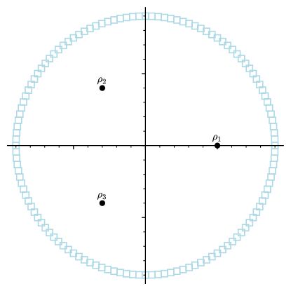
Figure 3. Covering the big circle with squares

Figure 4. Analytic continuation path

Inequality (17) implies that an upper bound for $\lim_{\varphi\to 0}|\mathcal{I}_{\mathcal{B}}|$ can be determined by finding some $C_{\mathcal{B}}>0$ such that

(44) $$\Bigl{|}f(z)-\sum_{\rho\in\Xi^{\mathrm{d}}}\ell_{\rho}(z)\Bigr{|}\leq C_{\mathcal{B}}\text{ whenever }|z|=R_{0}.$$

We cover the circle $\{|z|=R_{0}\}$ with small squares as illustrated in Figure 3, and compute approximations of $f(z)-\sum_{\rho\in\Xi^{\mathrm{d}}}\ell_{\rho}(z)$ on each square. The size of the squares should be small enough so that they do not contain any singularity of $\mathcal{D}$. For definiteness, we take squares of constant side length $\min_{\rho\in\Xi}|R_{0}-|\rho||/5$ which guarantees that the squares are sufficiently far away from singular points, helping to obtain bounds of reasonable size. (If $\min_{\rho\in\Xi}|R_{0}-|\rho||/5$ is very small, it is better to use a non-uniform covering to limit the number of small squares to be considered.)

Since we have explicit expressions for $\ell_{\rho}(z)$, we obtain enclosures of their ranges on each square by evaluations in ball arithmetic. It remains to bound $f(z)$ on each of the small squares. To do so we use a rigorous numerical solver for D-finite equations. The procedure is a simpler variant of the one used above to compute the connection matrices $\mathbf{C}_{0\rightarrow\rho}$ and deduce bounds on each $g_{\rho}(z)$ in the neighborhood of $\rho$. We construct paths in $\Delta_{\mathcal{D}}$ that connect the origin to each component of $\mathcal{B}$, making small detours to avoid singular points within $\Delta_{\mathcal{D}}$ if necessary, and then cover the corresponding component of $\mathcal{B}$ (see Figure 4). By solving the differential equation $\mathcal{D}f=0$ along these paths, we compute connection matrices from $0$ to the centers of the small squares covering $\mathcal{B}$. Finally, for each square we compute a few initial terms of the series expansion of $f$ at the center, evaluate them in interval arithmetic, and bound the remainder of the series using Proposition 5.1. This yields a bound of the form

$$|\mathcal{I}_{\mathcal{B}}|\leq C_{\mathcal{B}}R_{0}^{-n},$$

where $C_{\mathcal{B}}$ is the computed bound satisfying (44).

We note in passing that the rigorous numerical solver necessary for following the paths and computing the connection matrices can itself be realized using the same approach. Essentially, one discretizes the integration path and, at each step $z_{n}\to z_{n+1}$, computes approximations of $f(z_{n+1}),f^{\prime}(z_{n+1}),\dots,f^{(q-1)}(z_{n+1})$ by summing the Taylor expansion of $f$ at $z_{n}$. In the case of a D-finite equation, the coefficients of the Taylor series are easily generated using the associated recurrence. Computing a partial sum can be done in ball arithmetic, hence the critical issue for obtaining a rigorous enclosure of the solution is to bound the tails of each of the series, for which we can use Proposition 5.1 again (see [38] for details).

6.2. Combining the bounds

Now that we have bounds for each component in (16), it suffices to combine and simplify them to match the result given in Theorem 3.1.

We begin by computing the constant $N_{0}$ in Theorem 3.1. Firstly, in order for the integration path $\mathcal{P}(n)$ to be closed for all $n\geq N_{0}$, we require that $N_{0}\geq N_{1}$ where $N_{1}$ is defined in (10). Secondly, we need to guarantee the existence of an $s>2$ such that $N_{0}>s|\alpha|$ for all the exponents $\alpha$ to which we will apply the results of Sections 4 and 5 (Propositions 4.9 and 5.4). These exponents are of the form $\nu_{\rho,i}+r$ for some $\rho$, $i$, and $r\leq r_{0}$, where $r_{0}$ is the desired expansion order. Finally, the statement of the theorem specifies that $N_{0}\geq n_{0}$. Thus, we set

(45) $$N_{2}=\bigl{\lceil}2.1(\max_{\rho,i}\mathopen{|}\nu_{\rho,i}\mathclose{|}+r_{0}+1)\bigr{\rceil}\qquad\text{and}\qquad N_{0}=\max\left\{n_{0},N_{1},N_{2}\right\}.$$

Recall from (16) that we have

(46) $$f_{n}=[z^{n}]f(z)=\sum_{\rho\in\Xi^{\mathrm{d}}}[z^{n}]\ell_{\rho}+\sum_{\rho\in\Xi^{\mathrm{d}}}\frac{1}{2\pi\mathrm{i}}\int_{\mathcal{S}_{\rho}(n)+\mathcal{L}_{\rho}(n)}\frac{g_{\rho}(z)}{z^{n+1}}\,dz+\mathcal{I}_{\mathcal{B}},$$

and from (9) that we are aiming for a bound of the form

(47) $$f_{n}=\sum_{\rho\in\Xi^{\mathrm{d}}}\rho^{-n}n^{\gamma}\sum_{i=0}^{m_{\rho}}\sum_{k=0}^{\kappa}a_{\rho,i,k}\frac{\log^{k}n}{n^{\gamma_{\rho,i}}}+R(n),\qquad|R(n)|\leq A\,M^{-n}n^{\operatorname{Re}(\gamma)}\frac{\log^{\kappa}n}{n^{r_{0}}}.$$

In Sections 4 and 5 we computed a rigorous estimate for the first two sums in (46). This estimate can be viewed as a sum of monomials

(48) $$\mathbf{B}(a,\varepsilon)\cdot\rho^{-n}n^{\theta}\log^{k}n,$$

where $a\in\smash{\overline{\mathbb{Q}}}^{\mathrm{rhol},\Gamma}$ and the ball $\mathbf{B}(a,\varepsilon)$ is exact whenever $\operatorname{Re}(\theta)>\operatorname{Re}(\gamma)-r_{0}$. We call the terms such that $\operatorname{Re}(\theta)\leq\operatorname{Re}(\gamma)-r_{0}$ error terms, and those with $\operatorname{Re}(\theta)<\operatorname{Re}(\gamma)-r_{0}$ secondary error terms. In order to simplify the sum to the desired form, we need to identify $\gamma$ and trim down any secondary error terms that may appear. Let $\kappa$ be the maximum value of the parameter $k$ occurring among all error terms.

When $\operatorname{Re}(\theta)<\operatorname{Re}(\gamma)-r_{0}$, using the assumption $n\geq N_{0}$, we can replace a term of the form $\mathbf{B}(a,\varepsilon)\cdot\rho^{-n}n^{\theta}\log^{k}n$ with

(49) $$\mathbf{B}\left(0,(a+\varepsilon)\cdot N_{0}^{\operatorname{Re}(\theta)-\operatorname{Re}(\gamma)+r_{0}}\log^{k-\kappa}N_{0}\right)\cdot M^{-n}n^{\operatorname{Re}(\gamma)}\frac{\log^{\kappa}n}{n^{r_{0}}},$$

because

$$\mathbf{B}(a,\varepsilon)\cdot n^{\theta-\operatorname{Re}(\gamma)+r_{0}}\log^{k-\kappa}n\subseteq\mathbf{B}\left(0,(a+\varepsilon)\cdot N_{0}^{\operatorname{Re}(\theta)-\operatorname{Re}(\gamma)+r_{0}}\log^{k-\kappa}N_{0}\right)$$

when $n>N_{0}$. Replacing all secondary error terms in the sum of (48) with (49) standardizes all the error terms to the form $\mathbf{B}(0,a^{\prime})\cdot M^{-n}n^{\operatorname{Re}(\gamma)-r_{0}}\log^{\kappa}n$.

Remark 6.1.

Remarks 4.10 and 5.6 imply that, in some cases, the sum contains no error terms at all. When this happens, and if the next singular points of the differential equation by increasing modulus are also regular, one can subtract the sum of the corresponding local expansions from $f(z)$ and iterate the algorithm to improve the approximation of $f_{n}$ with exponentially smaller terms. It can also make sense to do something similar when the constant in the combined error term has been verified to be very small but could not be checked to be exactly zero for lack of a zero-test for connection coefficients.

In Section 6.1 we computed a bound for $\left|\mathcal{I}_{\mathcal{B}}\right|$ of the form $C_{\mathcal{B}}R_{0}^{-n}$. When $n\geq N_{0}$, letting $\beta=\operatorname{Re}(\gamma)-r_{0}$, we have

$$R_{0}^{-n}M^{n}n^{-\beta}\leq A=\begin{cases}e^{\beta}\left(\frac{\beta}{\log(M/R_{0})}\right)^{-\beta}&:\beta\leq N_{0}\log\frac{M}{R_{0}},\\ \left(\frac{M}{R_{0}}\right)^{N_{0}}N_{0}^{-\beta}&:\beta>N_{0}\log\frac{M}{R_{0}}.\end{cases}$$

In both cases, we can absorb $\mathcal{I}_{\mathcal{B}}$ into an error term of the form

$$\mathbf{B}\left(0,\frac{C_{\mathcal{B}}\,A}{\log^{\kappa}N_{0}}\right)\cdot M^{-n}n^{\operatorname{Re}(\gamma)-r_{0}}\log^{\kappa}n.$$

6.3. Proof of Theorem 3.1

Finally, we recall the statement of Theorem 3.1 and conclude its proof.

Theorem 3.1.

Let $M=\min_{\rho\in\Xi\setminus\Xi^{\mathrm{a}}}|\rho|$ be the minimal modulus of a singular point of $\mathcal{D}$, excluding any point where $f$ is known to be analytic. Algorithm 1 (page 1) computes an integer $N_{0}\geq n_{0}$ and an estimate

(50) $$f_{n}=\sum_{\rho\in\Xi^{\mathrm{d}}}\rho^{-n}n^{\gamma}\sum_{i=0}^{m_{\rho}}\sum_{k=0}^{\kappa}a_{\rho,i,k}\frac{\log^{k}n}{n^{\gamma_{\rho,i}}}+R(n),\quad|R(n)|\leq A\,M^{-n}n^{\operatorname{Re}(\gamma)}\frac{\log^{\kappa}n}{n^{r_{0}}}$$

for all $n\geq N_{0}$, where $0\leq\operatorname{Re}(\gamma_{\rho,0})\leq\operatorname{Re}(\gamma_{\rho,1})\leq\ldots\leq\operatorname{Re}(\gamma_{\rho,m_{\rho}})<r_{0}$. In this estimate, $\gamma$ and the $\gamma_{\rho,i}$ are algebraic numbers, the $a_{\rho,i,l}$ belong to the class $\smash{\overline{\mathbb{Q}}}^{\mathrm{rhol},\Gamma}$ and can be computed to arbitrary precision with rigorous error bounds, and $A$ is a nonnegative real number.

Proof.

The proof is a matter of checking that Algorithm 1 correctly implements the analysis from the previous sections. By Definition 3.4 and Proposition 3.5, we have

(51) $$[z^{n}]f(z)=\sum_{\rho\in\Xi^{\mathrm{d}}}\sum_{j=1}^{q}c_{\rho,j}\left([z^{n}]\ell_{\rho,j}(z)+\frac{1}{2\pi\mathrm{i}}\int_{\mathcal{S}_{\rho}(n)+\mathcal{L}_{\rho}(n)}\frac{g_{\rho,j}(z)}{z^{n+1}}\,dz\right)+\mathcal{I}_{\mathcal{B}}$$

where $c_{\rho,1},\dots,c_{\rho,q}$ are the coordinates of $f$ in the basis $(y_{\rho,j})_{j}$, the functions $\ell_{\rho,j}$ and $g_{\rho,j}$ are defined by (12)–(14) in terms of initial coefficients $d_{i,k,j}$ of the local expansion (5) of $y_{\rho,j}$, the paths $\mathcal{S}_{\rho}(n)$ and $\mathcal{L}_{\rho}(n)$ are defined in Section 3.2 and implicitly depend on $\varphi$, and $\mathcal{I}_{\mathcal{B}}$ is a quantity, also depending on $\varphi$, known to satisfy the inequality (17).

The algorithm essentially computes the terms of (51) one by one. Fix $\rho$ and $j$ and consider the corresponding terms.

As discussed in Section 2.3, since the path $0\to\rho$ is contained in the domain $\Delta_{\mathcal{D}}^{0}$ and $f$ is analytic on $\Delta_{\mathcal{D}}^{0}$, the coefficients $\mathbf{c}_{\rho}$ computed by steps (2) and (4b) agree with those appearing in (51). The parameters defining $\ell_{\rho,j}$ and $g_{\rho,j}$ are computed at steps (4a), 4(c)i, and 4(c)ii, by direct application of the definitions. In particular, after step 4(c)ii at each loop iteration, we have (cf. (4))

(52) $$[z^{n}]\ell_{\rho,j}(z)=\sum_{i=0}^{r_{j}-1}\sum_{k=0}^{\kappa_{j}}d_{i,k,j}\rho^{-n}[z^{n}](1-z)^{\nu_{j}+i}\log^{k}\left(\frac{1}{1-z}\right)$$

where all free variables on the right-hand side stand for computed values. The choice of $s$ at step 4(c)i ensures that $N_{0}>s\mathopen{|}\alpha\mathclose{|}$ at each call to Algorithm 2; hence, by Proposition 4.9, step 4(c)iii computes bounds that are valid for all $n\geq N_{0}$. It follows that, for each $\rho$ and $j$, step 4(c)iv yields a bound $E_{\rho,j}(n)$ for $[z^{n}]\ell_{\rho,j}$ also valid for all $n\geq N_{0}$.

Proposition 4.9 also states that, for each $(i,k)$, $e_{k}(n^{-1},\log n)$ has degree at most $\kappa_{j}$ with respect to $\log n$ and its coefficients of degree in $n^{-1}$ less than $r_{j}-i$ are elements of $\smash{\overline{\mathbb{Q}}}^{\mathrm{rhol},\Gamma}$. The choice of $r_{j}$ at step 4(c)i, referring to Definition 3.4, ensures that we have $\operatorname{Re}\nu_{j}+r_{j}+1\geq\lambda+r_{0}$ where $\lambda=\min_{j}\operatorname{Re}\nu_{j}$. This, combined with the algebraicity of $\rho$ and $d_{i,j,k}$, implies that the terms of $E_{\rho,j}(n)$ that are not contained in $O\bigl{(}n^{-\lambda-r_{0}}\log(n)^{\kappa_{j}}\bigr{)}$ have coefficients belonging to $\smash{\overline{\mathbb{Q}}}^{\mathrm{rhol},\Gamma}$.

Turning to the local error term, let

$$\mathcal{G}_{\rho,j}(n)=\frac{1}{2\pi\mathrm{i}}\lim_{\varphi\to 0}\int_{\mathcal{S}_{\rho}(n)+\mathcal{L}_{\rho}(n)}\frac{g_{\rho}(z)}{z^{n+1}}.$$

Step 4(c)v implements Remark 5.6: when $n_{j}$ is a nonnegative integer and $\kappa_{j}=0$, one can see from (14) that the function $z\mapsto g_{\rho}(z)z^{-n-1}$ is analytic at $\rho$, and hence on the disk $\{|z-\rho|\leq R_{1}\}$ defined by (11). As the path $\mathcal{S}_{\rho}(n)+\mathcal{L}_{\rho}(n)$ tends to a closed contour contained in this disk as $\varphi\to 0$, we have $\mathcal{G}_{\rho,j}(n)=0$ in this case. Otherwise steps 4(c)vi and 4(c)vii are executed. These steps are a direct application of Proposition 5.2 and Corollary 5.5. They yield a bound on $\mathcal{G}_{\rho,j}(n)$ of the form

$$O\bigl{(}n^{\operatorname{Re}\nu_{j}-1-r_{j}}\log(n)^{\kappa_{j}}\bigr{)}=O\bigl{(}n^{-\lambda-r_{0}}\log(n)^{\kappa_{j}}\bigr{)}$$

and valid for all $n\geq\max(N_{0},s\mathopen{|}\nu_{j}+r_{j}\mathclose{|})=N_{0}$.

Let $\mathcal{C}_{\mathcal{B}}\in\mathbb{R}_{\geq 0}$ denote the bound computed at step (5). By Equation (51) we have

$$\left|[z^{n}]\Bigl{(}f(z)-\sum_{\rho\in\Xi^{\mathrm{d}}}\sum_{j=1}^{q}c_{\rho,j}\ell_{\rho,j}(z)\Bigr{)}\right|\leq\sum_{\rho\in\Xi^{\mathrm{d}}}\sum_{j=1}^{q}c_{\rho,j}\left|\frac{1}{2\pi\mathrm{i}}\int_{\mathcal{S}_{\rho}(n)+\mathcal{L}_{\rho}(n)}\frac{g_{\rho,j}(z)}{z^{n+1}}\,dz\right|+\mathopen{|}\mathcal{I}_{\mathcal{B}}\mathclose{|}$$

for all small enough $\varphi>0$, and Equation (17) states that $\lim_{\varphi\to 0}\mathopen{|}\mathcal{I}_{\mathcal{B}}\mathclose{|}\leq R_{0}^{-n}\mathcal{C}_{\mathcal{B}}$ for $R_{0}$ given by (11) (which agrees with the value computed at step (3)). Therefore

(53) $$\left|[z^{n}]\left(f(z)-\sum_{\rho\in\Xi^{\mathrm{d}}}\sum_{j=1}^{q}c_{\rho,j}\ell_{\rho,j}(z)\right)\right|\leq\sum_{\rho\in\Xi^{\mathrm{d}}}\sum_{j=1}^{q}c_{\rho,j}\mathopen{|}\mathcal{G}_{\rho,j}(n)\mathclose{|}+\mathcal{C}_{\mathcal{B}}R_{0}^{-n}$$

for all $n\geq N_{0}$.

Finally, step (6) ensures that the output represents a bound of the form (50). More precisely, the simplification process sets $\gamma=-\nu_{j}$ for one of the $j$ such that $\operatorname{Re}\nu_{j}=\lambda$, and $\kappa=\max_{j}\kappa_{j}$. Combining the bounds $E_{\rho,j}(n)$ into the sum $\sum_{\rho\in\Xi^{\mathrm{d}}}\sum_{j=1}^{q}c_{\rho,j}E_{\rho,j}(n)$ yields an expression of the form (51). Since all contributions from steps 4(c)vii and (5) are in $O\bigl{(}n^{-\lambda-r_{0}}\log(n)^{\kappa_{j}}\bigr{)}$, adding them to $R(n)$ preserves its form. By (53), the resulting bound holds for all $n\geq N_{0}$. ∎

Remark 6.2.

In special circumstances, such as when dealing with algebraic series or diagonals, it is possible to express the coefficients in closed form. In particular, when dealing with an algebraic series, by choosing bases of solutions of $\mathcal{D}$ at the origin and at each singular point that are also solutions of the algebraic relation, the corresponding connection matrix (in Definition 2.10) is simply a permutation matrix. In this case, instead of dealing with coefficients in $\smash{\overline{\mathbb{Q}}}^{\mathrm{rhol},\Gamma}$, we only encounter elements of the $\overline{\mathbb{Q}}$-algebra generated by $\{\Gamma(\alpha)^{-1}:\alpha\in\overline{\mathbb{Q}}\}\cup\{\gamma^{(j)}(z):z\in\overline{\mathbb{Q}},j\in\mathbb{N}\}$.

7. Implementation and Further Examples

We have implemented the algorithm described in this article (up to minor variations) using the SageMath computer algebra system. Our implementation is part of the ore_algebra package [31], available at

https://github.com/mkauers/ore_algebra/

under the GNU General Public License. The version described here corresponds to git revision 47e05a45. The examples were run under SageMath 9.7.beta2. The documentation and test suite of ore_algebra contain executable versions of all examples from this paper, sometimes with minor changes.

Example 1.1 continued.

Using this version of ore_algebra, Example 1.1 (page Example 1.1 continued) can be reproduced through the following commands:

sage: from ore_algebra import OreAlgebra
sage: from ore_algebra.analytic.singularity_analysis import bound_coefficients
sage: Pol.<z> = PolynomialRing(QQ)
sage: Dop.<Dz> = OreAlgebra(Pol)  # Dz represents the operator d/dz
sage: dop = (z^2*(4*z - 1)*(4*z + 1)*Dz^3 + 2*z*(4*z+1)*(16*z-3)*Dz^2
....:        + 2*(112*z^2 + 14*z - 3)*Dz + 4*(16*z + 3))
sage: bound_coefficients(dop, [1, 2, 6], order=2)

On a standard laptop, the computation takes about 3.5 s, of which roughly 3 s are spent bounding the global error term by evaluation on the big circle.

The implementation builds on pre-existing code in ore_algebra for computing the connection matrices of Definition 2.10 (see [37]) and for computing bounds on tails of logarithmic series solutions of D-finite equations, as in Proposition 5.1 (see [38]). Except for singularities and local exponents, which are algebraic numbers and are represented exactly, numeric coefficients are represented as elements of SageMath’s ComplexBallField, based on the Arb library [26]. We perform intermediate computations that lead to the coefficients of the output at a working precision selected by the user, with the occasional addition of some guard digits for steps where we expect a loss of accuracy, but do not attempt to provide any guarantees on the radius of the output intervals. For operations that only affect the error terms, we currently use a fixed, hardcoded working precision. Our code also relies on SageMath’s AsymptoticRing [18] to represent the asymptotic expansion it outputs.

The implemented algorithm deviates from the one described here in some minor ways. Perhaps the most significant difference is that we implement the following variant of Remark 3.3: at step (4c) of Algorithm 1, elements $y_{j}$ of the local basis are partitioned according to their value modulo the integers of the exponent $\nu_{j}$, and the computations associated to of elements of a given class are carried out simultaneously.

Below we discuss some examples that illustrate the behaviour of our implementation on “real-life” P-recursive sequences. Except where noted, we call the algorithm with $r_{0}=2$, $n_{0}=50$, and an initial working precision of 53 bits. Taking $n_{0}=50$ makes the constants in the error terms slightly smaller than with the default $n_{0}=0$. There is room for improvement in the performance of the code: as of this writing, calls to bound_coefficients take about 2 to 15 seconds each on a standard laptop, with the vast majority of the time spent computing the global error term. All outputs were slightly edited for readability.

Example 7.1 (Diagonals of symmetric rational functions).

Due to a connection to certain special functions, Baryshnikov et al. [2] studied the diagonals of the family of rational functions $f(z_{1},\ldots,z_{d})=(1-(z_{1}+...+z_{d})+c\cdot z_{1}\ldots z_{d})^{-1}$ with $d\in\mathbb{N}$ and $c\in\mathbb{R}$, obtained by expanding $f(\mathbf{z})$ as a power series and taking the terms with monomials $(z_{1}z_{2}\cdots z_{d})^{n}$ where all exponents are equal. Taking $d=4$ and making the substitution $z_{1}z_{2}\cdots z_{d}=z$, the methods of creative telescoping imply that the operator [2, Equation 11]

$$\mathcal{D}= z^{2}(c^{4}z^{4}+4c^{3}z^{3}+6c^{2}z^{2}+4cz-256z+1)(3cz-1)^{2}\,\tfrac{d^{3}}{dz^{3}}$$

$$+3z(3cz-1)(6c^{5}z^{5}+15c^{4}z^{4}+8c^{3}z^{3}-6c^{2}z^{2}-384cz^{2}-6cz+384z-1)\,\tfrac{d^{2}}{dz^{2}}$$

$$+(cz+1)(63c^{5}z^{5}-3c^{4}z^{4}-66c^{3}z^{3}+18c^{2}z^{2}+720cz^{2}+19cz-816z+1)\,\tfrac{d}{dz}$$

$$+(9c^{6}z^{5}-3c^{5}z^{4}-6c^{4}z^{3}+18c^{3}z^{2}-360c^{2}z^{2}+13c^{2}z-384cz+c-24)$$

annihilates the diagonal $f_{\mathrm{diag}}(z)$. Baryshnikov et al. showed that $f_{\mathrm{diag}}(z)$ is ultimately positive if and only if $c<(d-1)^{d-1}$, with certain interesting phenomena happening at $c=(d-1)^{d-1}$. We illustrate this result for $d=4$ and $c\in\{28,27,26\}$.

When $c=28$:

The diagonal $f_{\mathrm{diag}}(z)$ has the initial coefficient sequence $(f_{0},f_{1},f_{2})=(1,-4,-56)$. Our implementation returns

$$f_{n} \in\phi^{n}n^{-3/2}\cdot\bigl{(}\begin{aligned} &([-0.0311212622056357\pm 10^{-16}]+[-0.0345183803114027\pm 10^{-16}]\mathrm{i})\\ &+([0.050269964085834\pm 10^{-15}]+[-0.0298161277530909\pm 10^{-16}]\mathrm{i})\,n^{-1}\bigr{)}\end{aligned}$$

$$\phantom{\in}+\overline{\phi}^{n}n^{-3/2}\cdot\bigl{(}\begin{aligned} &([-0.0311212622056357\pm 10^{-16}]+[0.0345183803114027\pm 10^{-16}]\mathrm{i})\\ &+([0.050269964085834\pm 10^{-15}]+[0.0298161277530909\pm 10^{-16}]\mathrm{i})\,n^{-1}\bigr{)}\end{aligned}$$

$$\phantom{\in}+B(6.11\,|\phi|^{n}n^{-7/2},n\geq 50)$$

where $\phi\approx 79.33+25.48i$ is algebraic of degree $4$ and $B(\varepsilon_{n},n\geq N_{0})$ indicates an term of absolute value bounded by $\varepsilon_{n}$ for all $n\geq N_{0}$. In this case, $f_{n}$ is not ultimately positive.

When $c=27$:

In this case $(f_{0},f_{1},f_{2})=(1,-3,9)$, and our implementation returns

$$f_{n} \in\phi^{n}n^{-3/2}\cdot\bigl{(}\begin{aligned} &([0.306608607103967\pm 10^{-15}]+[0.146433894558384\pm 10^{-15}]\mathrm{i})\\ &+([-0.26554984277221\pm 10^{-15}]+[-0.03529869348794\pm 10^{-15}]\mathrm{i})n^{-1}\bigr{)}\end{aligned}$$

$$\phantom{\in}+\overline{\phi}^{n}n^{-3/2}\cdot\bigl{(}\begin{aligned} &([0.306608607103967\pm 10^{-15}]+[-0.146433894558384\pm 10^{-15}]\mathrm{i})\\ &+([-0.26554984277221\pm 10^{-15}]+[0.03529869348794\pm 10^{-15}]\mathrm{i})n^{-1}\bigr{)}\end{aligned}$$

$$\phantom{\in}+B(50.1\,\cdot\,9^{n}n^{-7/2},n\geq 50)$$

where one can check that $\phi=-7+4\sqrt{2}\mathrm{i}$. In this case $f_{n}$ is also not ultimately positive, however an interesting phenomenon observed in [2] is explicitly illustrated here: as $c\to 27$ the exponential growth rate of $|f_{n}|$ drops from around 81 to 9.

When $c=26$:

One has $(f_{0},f_{1},f_{2})=(1,-2,76)$, and our implementation gives

$$f_{n}\in\phi^{n}\cdot\bigl{(}\begin{aligned} &[0.0484997667050581\pm 10^{-16}]n^{-3/2}+[-0.068160009777454\pm 10^{-15}]n^{-5/2}\\ &+B(8.41\,n^{-7/2},n\geq 50)\bigr{)}\end{aligned}$$

for a real algebraic number $\phi\approx 108.10$ of degree $4$. From this, we can immediately see that $f_{n}$ is positive for all $n\geq 50$, verifying the ultimate positivity derived in [2] using multivariate methods.

Next, we give an example that illustrates how our algorithm deals with complex exponents.

Example 7.2 (Complex exponents).

Consider the power series $f(z)=f_{0}+f_{1}z+f_{2}z^{2}+\cdots$ with the initial conditions $(f_{0},f_{1},f_{2})=\left(1,2,-1/8\right)$ satisfying $\mathcal{D}f=0$ where

$$\mathcal{D}=(z-2)^{2}\frac{d^{2}}{dz^{2}}+z(z-2)\frac{d}{dz}+1.$$

Algorithm 1 finds that

$$f_{n}\in 2^{-n}\cdot\bigl{(}\begin{aligned} &([1.1243375066147\pm 10^{-14}]+[-0.4622196104635\pm 10^{-14}]\mathrm{i}){n^{-\alpha\mathrm{i}-1/2}}\\ &+([1.1243375066147\pm 10^{-14}]+[-0.4622196104635\pm 10^{-14}]\mathrm{i}){n^{\alpha\mathrm{i}-1/2}}\\ &+([-0.4002939247887\pm 10^{-14}]+[-0.9737048431560\pm 10^{-14}]\mathrm{i}){n^{-\alpha\mathrm{i}-3/2}}\\ &+([-0.4002939247887\pm 10^{-14}]+[0.9737048431560\pm 10^{-14}]\mathrm{i}){n^{\alpha\mathrm{i}-3/2}}\\ &+B(9\cdot 10^{3}\,n^{-5/2},n_{0}\geq 50)\bigr{)},\end{aligned}$$

with $\alpha=\frac{\sqrt{3}}{2}$. We can conclude in particular that the series $(f_{n})$ is not ultimately positive, since for any $\varepsilon>0$, there exist infinitely many $n$ such that $\arg(n^{\alpha\mathrm{i}})\in(\pi-\varepsilon,\pi)$.

The following example from [32] illustrates how a priori knowledge about dominant singularities can affect the usefulness of the bound produced.

Example 7.3 (Difficulty of certifying singularities).

Consider the sequence $(f_{n})$ with the initial conditions $(f_{0},f_{1})=\left(1,\frac{1}{4}\right)$ satisfying the recurrence equation

$$(n+3)^{2}f_{n+2}-\frac{1}{2}(n+2)(3n+11)f_{n+1}+\frac{1}{2}(n+4)(n+1)f_{n}=0.$$

The generating function $f(z)$ of $\{f_{n}\}$ is a solution of the operator

$$\mathcal{D}=\left(\frac{1}{2}z^{4}-\frac{3}{2}z^{3}+z^{2}\right)\frac{d^{4}}{dz^{4}}+\left(7z^{3}-16z^{2}+7z\right)\frac{d^{3}}{dz^{3}}+\left(26z^{2}-41z+9\right)\frac{d^{2}}{dz^{2}}+\left(26z-22\right)\frac{d}{dz}+4.$$

Without any a priori knowledge of dominant singularities of $f$, the algorithm assumes the singular point of $\mathcal{D}$ with the smallest modulus apart from 0, which is $z=1$, to be the dominant singularity of $f$. Our implementation, with the initial working precision raised to 1000 bits, determines that

$$f_{n}\in[\pm 10^{-300}]+[\pm 10^{-300}]\mathrm{i}+B(3\cdot 10^{3}\,(4/7)^{n},n\geq 50)$$

This estimate does not give much useful information about the asymptotic behaviour of $f_{n}$, since we do not know if the dominant term is zero or not. The output suggests however that the corresponding constant might indeed be zero, in other words, that $f$ might be analytic at $z=1$. A direct computation shows that indeed $f_{n}=\frac{2^{-n}}{n+1}$ and $f(z)=\frac{1}{2}\log\frac{1}{1-z/2}$.

Adding $\Xi^{\mathrm{a}}=\{0,1\}$ to the input of Algorithm 1 results in the bound

$$f_{n}\in 2^{-n}\cdot\bigl{(}[1.0\pm 10^{-15}]n^{-1}+([1.0\pm 10^{-15}])n^{-2}+B(66\,n^{-3}\log n,n\geq 50)\bigr{)},$$

which characterizes the dominant asymptotic behaviour of $f_{n}$.

References

• [1] My Abdelfattah Barkatou “Contribution à l’étude des équations différentielles et aux différences dans le champ complexe”, 1989
• [2] Yuliy Baryshnikov, Stephen Melczer, Robin Pemantle and Armin Straub “Diagonal Asymptotics for Symmetric Rational Functions via ACSV” In 29th International Conference on Probabilistic, Combinatorial and Asymptotic Methods for the Analysis of Algorithms, AofA 2018, June 25-29, 2018, Uppsala, Sweden 110, LIPIcs Schloss Dagstuhl - Leibniz-Zentrum für Informatik, 2018, pp. 12:1–12:15 DOI: 10.4230/LIPIcs.AofA.2018.12
• [3] George D. Birkhoff “Formal Theory of Irregular Linear Difference Equations” In Acta Mathematica, 1930
• [4] George D. Birkhoff and Waldemar J. Trjitzinsky “Analytic theory of singular difference equations” In Acta mathematica 60.1 Springer, 1933, pp. 1–89
• [5] Alin Bostan and Sergey Yurkevich “A hypergeometric proof that $\mathsf{Iso}$ is bijective” In Proceedings of the American Mathematical Society 150.5, 2022, pp. 2131–2136 DOI: 10.1090/proc/15836
• [6] Mireille Bousquet-Mélou “Rational and algebraic series in combinatorial enumeration” In International Congress of Mathematicians. Vol. III Eur. Math. Soc., Zürich, 2006, pp. 789–826
• [7] Richard P. Brent “Fast multiple precision evaluation of elementary functions” In Journal of the ACM 23, 1976, pp. 242–251 URL: http://wwwmaths.anu.edu.au/~brent/pub/pub034.html
• [8] Cyril Chabaud “Séries génératrices algébriques : asymptotique et applications combinatoires”, 2002
• [9] Ruiwen Dong “Asymptotic Expansion and Error Bounds of P-Recursive Sequences”, 2021
• [10] Anne Duval “Solutions irrégulières d’équations aux differences polynomiales” In Équations différentielles et systèmes de Pfaff dans le champ complexe — II 1015 Springer, 1983, pp. 64–101 DOI: 10.1007/BFb0071350
• [11] Philippe Flajolet and Andrew Odlyzko “Singularity analysis of generating functions” In SIAM Journal on discrete mathematics 3.2 SIAM, 1990, pp. 216–240
• [12] Philippe Flajolet and Claude Puech “Partial match retrieval of multidimensional data” In Journal of the ACM 33.2, 1986, pp. 371–407 URL: http://algo.inria.fr/flajolet/Publications/FlPu86.pdf
• [13] Philippe Flajolet, Bruno Salvy and Paul Zimmermann “Automatic Average-case Analysis of Algorithms” In Theoretical Computer Science 79.1, 1991, pp. 37–109 URL: http://hal.inria.fr/inria-00077102_v1/
• [14] Philippe Flajolet and Robert Sedgewick “Analytic combinatorics” Cambridge University Press, Cambridge, 2009
• [15] Philippe Flajolet and Brigitte Vallée “Continued Fractions, Comparison Algorithms, and Fine Structure Constants” In Constructive, experimental, and nonlinear analysis American Mathematical Society, 2000, pp. 53–82
• [16] C.L. Frenzen “Error bounds for the asymptotic expansion of the ratio of two Gamma functions with complex argument” In SIAM Journal on Mathematical Analysis 23.2 SIAM, 1992, pp. 505–511
• [17] Stefan Gerhold and Manuel Kauers “A Procedure for Proving Special Function Inequalities Involving a Discrete Parameter” In Proceedings of the 2005 International Symposium on Symbolic and Algebraic Computation, ISSAC ’05 New York, NY, USA: Association for Computing Machinery, 2005, pp. 156–162 DOI: 10.1145/1073884.1073907
• [18] Benjamin Hackl, Clemens Heuberger and Daniel Krenn “Asymptotic expansions in SageMath” module in SageMath 6.10, 2015 URL: http://trac.sagemath.org/17601
• [19] Joris Hoeven “Efficient accelero-summation of holonomic functions” In Journal of Symbolic Computation 42.4, 2007, pp. 389–428 URL: http://www.texmacs.org/joris/reshol/reshol-abs.html
• [20] Joris Hoeven “Efficient accelero-summation of holonomic functions” Corrected version of [19], 2021 URL: https://hal.archives-ouvertes.fr/hal-03154241
• [21] Joris Hoeven “Fast Evaluation of Holonomic Functions Near and in Regular Singularities” In Journal of Symbolic Computation 31.6, 2001, pp. 717–743 URL: http://www.texmacs.org/joris/singhol/singhol-abs.html
• [22] Joris Hoeven “Fuchsian holonomic sequences”, 2021 URL: https://hal.archives-ouvertes.fr/hal-03291372
• [23] Hui Huang and Manuel Kauers “D-finite numbers” In Int. J. Number Theory 14.7, 2018, pp. 1827–1848
• [24] G.. Immink “Reduction to canonical forms and the Stokes phenomenon in theory of linear difference equations” In SIAM Journal on Mathematical Analysis 22.1 SIAM, 1991, pp. 238–259
• [25] Geertrui Klara Immink “On the relation between linear difference and differential equations with polynomial coefficients” In Mathematische Nachrichten 200.1 Wiley Online Library, 1999, pp. 59–76
• [26] Fredrik Johansson “Arb: Efficient arbitrary-precision midpoint-radius interval arithmetic” In IEEE Transactions on Computers 66.8 IEEE, 2017, pp. 1281–1292 DOI: 10.1109/TC.2017.2690633
• [27] Sébastien Julliot “Automatic Asymptotics for Combinatorial Series”, 2020
• [28] Reinwald Jungen “Sur les séries de Taylor n’ayant que des singularités algébrico-logarithmiques sur leur cercle de convergence” In Commentarii Mathematici Helvetici 3.1 Springer, 1931, pp. 266–306
• [29] E.. Karatsuba “Fast computation of the values of the Hurwitz zeta function and Dirichlet L-series” In Problemy Peredachi Informatsii 34.4, 1998, pp. 62–75
• [30] Manuel Kauers “A Mathematica package for computing asymptotic expansions of solutions of P-finite recurrence equations”, 2011
• [31] Manuel Kauers, Maximilian Jaroschek and Fredrik Johansson “Ore polynomials in Sage” In Computer algebra and polynomials 8942, Lecture Notes in Comput. Sci. Springer, Cham, 2015, pp. 105–125
• [32] Manuel Kauers and Veronika Pillwein “When can we detect that a P-finite sequence is positive?” In ISSAC 2010—Proceedings of the 2010 International Symposium on Symbolic and Algebraic Computation ACM, New York, 2010, pp. 195–201 DOI: 10.1145/1837934.1837974
• [33] George Kenison et al. “On Positivity and Minimality for Second-Order Holonomic Sequences” In 46th International Symposium on Mathematical Foundations of Computer Science, MFCS 2021, August 23-27, 2021, Tallinn, Estonia 202, LIPIcs, 2021, pp. 67:1–67:15 DOI: 10.4230/LIPIcs.MFCS.2021.67
• [34] Stephen Melczer “An Invitation to Analytic Combinatorics: From One to Several Variables”, Texts and Monographs in Symbolic Computation Springer International Publishing, 2021
• [35] Stephen Melczer and Marc Mezzarobba “Sequence Positivity Through Numeric Analytic Continuation: Uniqueness of the Canham Model for Biomembranes” In Combinatorial Theory 2.2, 2022
• [36] Marc Mezzarobba “Autour de l’évaluation numérique des fonctions D-finies”, 2011 URL: http://tel.archives-ouvertes.fr/pastel-00663017/
• [37] Marc Mezzarobba “Rigorous Multiple-Precision Evaluation of D-Finite Functions in SageMath”, 2016 URL: https://arxiv.org/abs/1607.01967
• [38] Marc Mezzarobba “Truncation bounds for differentially finite series” In Annales Henri Lebesgue 2, 2019, pp. 99–148
• [39] Gopal Mohanty “Lattice path counting and applications” Academic Press, 2014
• [40] G. Nemes “Error bounds for the asymptotic expansion of the Hurwitz zeta function” In Proceedings of the Royal Society A: Mathematical, Physical and Engineering Sciences 473.2203 Royal Society, 2017, pp. 20170363 DOI: 10.1098/rspa.2017.0363
• [41] Eike Neumann, Joël Ouaknine and James Worrell “Decision Problems for Second-Order Holonomic Recurrences” In 48th International Colloquium on Automata, Languages, and Programming (ICALP 2021) 198, Leibniz International Proceedings in Informatics (LIPIcs), 2021, pp. 99:1–99:20 DOI: 10.4230/LIPIcs.ICALP.2021.99
• [42] Andrew M. Odlyzko “Asymptotic Enumeration Methods” In Handbook of Combinatorics 2 Elsevier, 1995, pp. 1063–1229 URL: http://www.dtc.umn.edu/~odlyzko/doc/asymptotic.enum.pdf
• [43] F… Olver “Asymptotics and special functions” A K Peters, 1997
• [44] Joël Ouaknine and James Worrell “Positivity Problems for Low-Order Linear Recurrence Sequences” In Proceedings of the Twenty-Fifth Annual ACM-SIAM Symposium on Discrete Algorithms Society for IndustrialApplied Mathematics, 2014, pp. 366–379 DOI: 10.1137/1.9781611973402.27
• [45] Veronika Pillwein “Termination Conditions for Positivity Proving Procedures” In Proceedings of the 38th International Symposium on Symbolic and Algebraic Computation, ISSAC ’13 New York, NY, USA: Association for Computing Machinery, 2013, pp. 315–322 DOI: 10.1145/2465506.2465945
• [46] S. Pincherle “Sur la génération de systèmes récurrents au moyen d’une équation linéaire différentielle” In Acta Math. 16.1, 1892, pp. 341–363
• [47] E… Poole “Introduction to the theory of linear differential equations” Dover Publications, Inc., New York, 1960
• [48] Marius Put and Michael F. Singer “Galois theory of difference equations” 1666, Lecture Notes in Mathematics Berlin: Springer, 1997
• [49] Bruno Salvy “Asymptotique automatique et fonctions génératrices”, 1991 URL: https://www.theses.fr/1991EPXX0007
• [50] Bruno Salvy “Fonctions génératrices et asymptotique automatique”, 1989 URL: https://hal.inria.fr/inria-00075592
• [51] Évelyne Tournier “Solutions formelles d’équations différentielles”, 1987 URL: http://tel.archives-ouvertes.fr/tel-00323706/fr/
• [52] Francesco Giacomo Tricomi and Arthur Erdélyi “The asymptotic expansion of a ratio of gamma functions.” In Pacific Journal of Mathematics 1.1, 1951, pp. 133–142
• [53] Thomas Yu and Jingmin Chen “Uniqueness of Clifford torus with prescribed isoperimetric ratio” In Proc. Amer. Math. Soc. 150.4, 2022, pp. 1749–1765
• [54] Doron Zeilberger “AsyRec: A Maple package for Computing the Asymptotics of Solutions of Linear Recurrence Equations with Polynomial Coefficients”, 2008 URL: http://www.math.rutgers.edu/~zeilberg/mamarim/mamarimhtml/asy.html