QVIP: An ILP-based Formal Verification Approach
for Quantized Neural Networks

Abstract.

Deep learning has become a promising programming paradigm in software development, owing to its surprising performance in solving many challenging tasks. Deep neural networks (DNNs) are increasingly being deployed in practice, but are limited on resource-constrained devices owing to their demand for computational power. Quantization has emerged as a promising technique to reduce the size of DNNs with comparable accuracy as their floating-point numbered counterparts. The resulting quantized neural networks (QNNs) can be implemented energy-efficiently. Similar to their floating-point numbered counterparts, quality assurance techniques for QNNs, such as testing and formal verification, are essential but are currently less explored. In this work, we propose a novel and efficient formal verification approach for QNNs. In particular, we are the first to propose an encoding that reduces the verification problem of QNNs into the solving of integer linear constraints, which can be solved using off-the-shelf solvers. Our encoding is both sound and complete. We demonstrate the application of our approach on local robustness verification and maximum robustness radius computation. We implement our approach in a prototype tool QVIP and conduct a thorough evaluation. Experimental results on QNNs with different quantization bits confirm the effectiveness and efficiency of our approach, e.g., two orders of magnitude faster and able to solve more verification tasks in the same time limit than the state-of-the-art methods.

1. Introduction

Deep neural networks (DNNs) have gained widespread attention as a promising programming paradigm thanks to their surprising performance in solving various complicated tasks (Karpathy et al., 2014; Hinton et al., 2012; Pennington et al., 2014). DNNs are increasingly being deployed in software applications such as autonomous driving (Apollo, 2018) and medical diagnostics (Ciresan et al., 2012), and have become a subject of intensive software engineering research.

Modern DNNs usually contain a great number of parameters which are typically stored as 32/64-bit floating-point numbers, and require a massive amount of floating-point operations to compute the outputs at running time (Tan and Le, 2019). Hence, modern DNNs are both memory intensive and computationally intensive, making them difficult to deploy on energy- and computation-constrained devices (Han et al., 2016). To address this issue, compression techniques have been proposed to ‘deflate’ DNNs by removing redundant connections and quantizing parameters from 32/64-bit floating-points to lower bit-width fixed-points (e.g., 8-bits) (Han et al., 2016; Jacob et al., 2018), which can vastly reduce the memory requirement and computational cost based on bit-wise and/or integer-only arithmetic computations. For instance, Tesla’s Full Self-Driving Chip (previously Autopilot Hardware 3.0) is designed for primarily running 8-bit quantized DNNs (Henzinger et al., 2021; WikiChip, 2022). Quantization is also made available to ordinary programmers through popular deep learning frameworks. For instance, TensorFlow Lite (TFL, 2022) supports, among others, 8-bit quantization on parameters.

Despite their great success, DNNs are known to be vulnerable to input perturbations due to the lack of robustness (Carlini and Wagner, 2017; Papernot et al., 2016; Goodfellow et al., 2015; Kurakin et al., 2017; Szegedy et al., 2014; Song et al., 2021; Chen et al., 2021a; Bu et al., 2021; Chen et al., 2022a, b, 2021b). This is concerning as such errors may lead to catastrophes when DNNs are deployed in safety-critical applications. For example, a self-driving car may misclassify a stop sign as a speed-limit sign (Eykholt et al., 2018). As a result, along with traditional verification and validation (V&V) research in software engineering, there is a large and growing body of work on developing V&V techniques for DNNs, which has become a focus of software engineering researchers. For instance, testing techniques have been proposed to evaluate robustness of DNNs against input perturbations, e.g., (Carlini and Wagner, 2017; Ma et al., 2018a, b; Pei et al., 2017; Sun et al., 2018; Tian et al., 2018; Xie et al., 2019a; Odena et al., 2019; Xie et al., 2019b), cf. (Zhang et al., 2022a) for a survey. Such techniques are often effective in finding input samples to demonstrate lack of robustness, but they cannot prove the absence of such inputs. Many efforts have also been made to formally verify the robustness of DNNs (Pulina and Tacchella, 2010; Katz et al., 2017; Gehr et al., 2018; Huang et al., 2017; Singh et al., 2019b; Wang et al., 2018; Tran et al., 2019; Elboher et al., 2020; Yang et al., 2021; Liu et al., 2020; Guo et al., 2021; Zhao et al., 2022; Liu et al., 2022), to cite a few. In general, we advocate the research on quality assurance for DNNs, which are increasingly a component of modern software systems, to which our current work contributes to.

Almost all the existing work is designated for real or floating-point numbered DNNs only whereas verification of quantized DNNs (QNNs) has not been thoroughly investigated yet, although there is a gap of verification results between real-numbered DNNs and their quantized counterparts due to the fixed-point semantics of QNNs (Giacobbe et al., 2020). Thus, there is a growing need for the research of quality assurance techniques for QNNs. One possible approach to verify QNNs is to adopt differential verification (Lahiri et al., 2013) which was initially proposed for verifying a new version of a program with respect to a previous version. One could first verify a real or floating-point numbered DNN by applying existing techniques and then verify its quantized counterpart by applying differential verification techniques for DNNs (Paulsen et al., 2020a, b; Mohammadinejad et al., 2021). However, it has two drawbacks. First, existing differential verification techniques for DNNs (Paulsen et al., 2020a, b; Mohammadinejad et al., 2021) are incomplete, and thus may produce false positives even if the original DNN is robust. Second, quantization introduces non-monotonicity on the output of DNNs (Giacobbe et al., 2020), consequently, a robust DNN may become non-robust after quantization while a non-robust DNN may become a robust QNN. Therefore, dedicated techniques are required for directly and rigorously verifying QNNs.

There do exist techniques for directly verifying QNNs which leverage Boolean Satisfiability (SAT) or Satisfiability Modulo Theory (SMT) solving or (reduced, ordered) binary decision diagrams (BDDs). For 1-bit quantized DNNs, i.e., Binarized Neural Networks (BNNs), Narodytska et al. (Narodytska et al., 2018) proposed to translate the BNN verification problem into the satisfiability problem of Boolean formulas where SAT solving is harnessed. Using a similar encoding, Baluta, et al. (Baluta et al., 2019) proposed to quantitatively verify BNNs via approximate model counting. Following this direction, Shih et al. (Shih et al., 2019b, a) proposed a BDD learning-based approach to quantitatively analyze BNNs, and Zhang et al. (Zhang et al., 2021) introduced an efficient BDD encoding method by exploiting the internal structure of BNNs. Recently, the SMT-based verification framework Marabou has also been extended to support BNNs (Amir et al., 2020). For quantization with multiple bits (e.g., fixed-point), methods also have been proposed (Baranowski et al., 2020; Giacobbe et al., 2020; Henzinger et al., 2021), which reduce the verification problem of QNNs to SMT solving accounting for the fixed-point semantics of QNNs. They are sound and complete, but have fairly limited scalability.

In this work, we propose the first integer linear programming (ILP) based verification approach for QNNs. To this end, we present a novel and exact encoding which precisely reduces the verification problem for QNNs to an integer linear programming program. More specifically, we propose to use piecewise constant functions to encode piecewise linear activation functions that are computations of neurons in QNNs. The piecewise constant functions are further encoded as integer linear constraints with the help of additional Boolean variables. We also propose encodings to express desired input space and robustness properties using integer linear constraints. The number of integer linear constraints produced by our encoding method is linear (at most 4 times) in the number of neurons of QNNs. Based on our encoding, we develop a theoretically complete and practically efficient verification framework for QNNs. To further improve the scalability and efficiency, we leverage interval analysis to soundly approximate the neuron outputs, which can effectively reduce the size of integer linear constraints and number of Boolean variables, and consequently, reduce verification cost. We highlight two applications of our approach, i.e., robustness verification and computation of maximum robustness radii.

We implement our approach as an end-to-end tool, named QVIP, with Gurobi (Gurobi, 2018) as the underlying ILP-solver. We extensively evaluate QVIP on various QNNs with different quantization bits using two popular datasets MNIST (LeCun and Cortes, 2010) and Fashion-MNIST (Xiao et al., 2017), where the number of neurons varies from 858 to 894, and the number of bits for quantizing parameters ranges from 4 to 10 bits with 8-bit input quantization. For robustness verification, experimental results show that our approach is two orders of magnitude faster and is able to solve more verification tasks within the same time limit than the state-of-the-art verifier for multiple-bit QNNs (Henzinger et al., 2021). To the best of our knowledge, QVIP is the first tool that can handle input spaces with an attack radius up to 30 for robust verification of QNNs. Interestingly, we found that, although the accuracy of the QNNs stays similar under different quantization bits, the robustness can be greatly improved with more quantization bits using quantization-aware training (Jacob et al., 2018). We remark that Giacobbe et al. (Giacobbe et al., 2020) showed that neither robustness nor non-robustness is monotonic with the number of quantization bits using post-training quantization (Nagel et al., 2021). This suggests that robustness should also be considered, in addition to accuracy, during quantization-aware training which is able to produce more accurate QNNs than post-training quantization. Furthermore, we show the effectiveness of QVIP in computing maximum robustness radii based on binary search. Experimental results show that it can be utilized to compare the overall robustness of QNNs with different quantization bits.

To summarize, our main contributions are as follows.

• We propose the first ILP-based verification approach for QNNs featuring both precision and efficiency.

• We implement our approach as an end-to-end tool QVIP, using the ILP-solver Gurobi for QNN robustness verification and maximum robustness radius computation.

• We conduct an extensive evaluation of QVIP, demonstrating the efficiency and effectiveness of QVIP, e.g., significantly outperforming the state-of-the-art methods.

Outline. We define QNNs and problems in Section 2. In Section 3, we propose the ILP-based verification approach. In Section 4, we present an algorithm for computing maximum robustness radii. We report our experimental results in Section 5. Section 6 discusses related work. Finally, we conclude in Section 7.

To foster further research, benchmarks and experimental data are released on our website (Zhang et al., 2022b).

2. Preliminaries

We denote by $\mathbb{R}$, $\mathbb{N}$, $\mathbb{Z}$ and $\mathbb{B}$ the set of real numbers, natural numbers, integers and Boolean domain $\{0,1\}$ respectively. Given a number $n\in\mathbb{N}$, let $[n]:=\{1,\cdots,n\}$, $\mathbb{R}^{n}$ and $\mathbb{Z}^{n}$ be the sets of the $n$-tuples of real numbers and integers, respectively. We use ${\mathbf{W}},{\mathbf{W^{\prime}}},\ldots$ to denote matrices, ${\mathbf{x}},{\mathbf{y}},\ldots$ to denote vectors, and $x,y,\dots$ to denote scalars. We denote by ${\mathbf{W}}_{i,:}$ and ${\mathbf{W}}_{:,j}$ the $i$-th row and $j$-th column of the matrix ${\mathbf{W}}$. Similarly, we denote by ${\mathbf{x}}_{j}$ and ${\mathbf{W}}_{i,j}$ the $j$-th entry of ${\mathbf{x}}$ and ${\mathbf{W}}_{i,:}$ respectively.

2.1. Deep Neural Networks

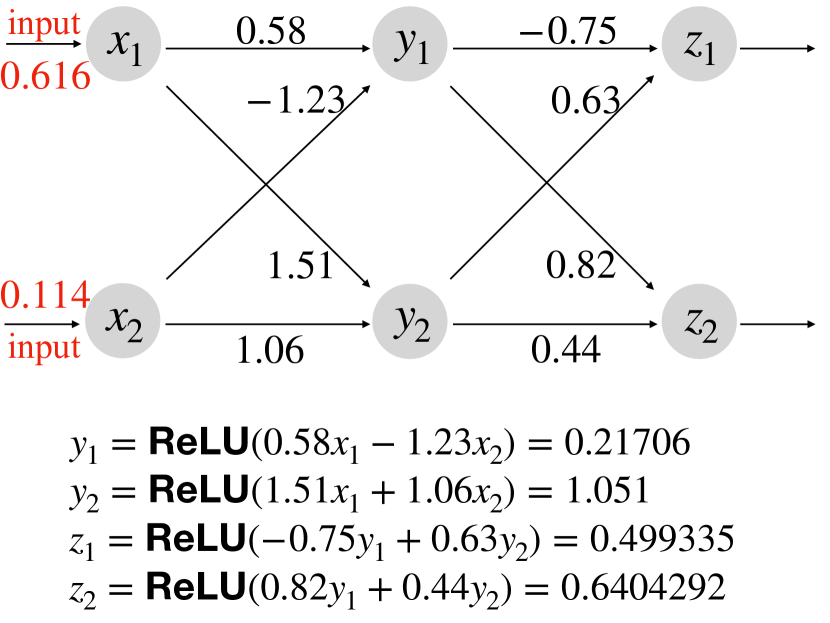
(a) DNN $\mathcal{N}_{e}$.

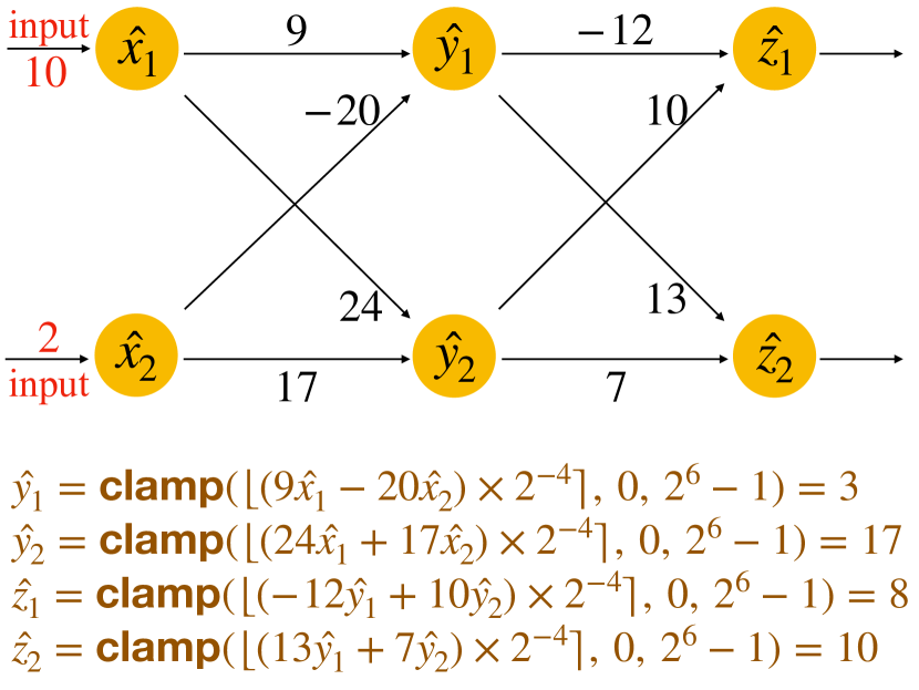
(b) QNN $\widehat{\mathcal{N}}_{e}$.

Figure 1. A 3-layer DNN ${\mathcal{N}}_{e}$ and its quantized version $\widehat{\mathcal{N}}_{e}$.

A deep neural network (DNN) $\mathcal{N}$ is a graph structured in layers, where the first layer is the input layer, the last layer is the output layer, and the others are hidden layers. All the nodes in these layers are called neurons (in particular, neurons in hidden layers are called hidden neurons). Each neuron in a non-input layer is associated with a bias and could be connected by other neurons via weighted, directed edges. A DNN is feed-forward if all the neurons only point to neurons in the next layer. In this work, we focus on feed-forward DNNs. Given an input, a DNN computes an output by propagating it through the network layer by layer, where the value of each neuron is computed by applying an activation function to the weighted sum of output values from the preceding layer or input.

A DNN $\mathcal{N}$ with $d$ layers is a function $\mathcal{N}:\mathbb{X}\rightarrow\mathbb{Y}$, where $\mathbb{X}\subseteq\mathbb{R}^{n}$ is the input domain and $\mathbb{Y}\subseteq\mathbb{R}^{m}$ is the output domain. For any input ${\mathbf{x}}\in\mathbb{X}$, $\mathcal{N}({\mathbf{x}})={\mathbf{W}}^{d}{\mathbf{y}}^{d-1}+{\mathbf{b}}^{d}$, where ${\mathbf{y}}^{d-1}$ is obtained by the following recursive definition:

$\begin{aligned} {\mathbf{y}}^{1}={\mathbf{x}},\qquad{\mathbf{y}}^{i}=\sigma({\mathbf{W}}^{i}{\mathbf{y}}^{i-1}+{\mathbf{b}}^{i})\quad\mbox{for}\ i=2,\ldots,d-1,\\ \end{aligned}$

where ${\mathbf{W}}^{i}$ and ${\mathbf{b}}^{i}$ (for $2\leq i\leq d$) are the weight matrix and bias vector of the $i$-th layer respectively, and $\sigma$ is an activation function (e.g., ReLU, sigmoid) applied to the vector entrywise. In this work, we focus on the most commonly used one ${\tt ReLU}(x)=\max(x,0)$.

For classification tasks, the output class of a given input ${\mathbf{x}}$, denoted by $\mathcal{N}^{c}({\mathbf{x}})$, is the first index of $\mathcal{N}({\mathbf{x}})$ with the highest value.

Example 2.1.

Figure 1(a) shows a running example DNN $\mathcal{N}_{e}$ with 3 layers, where each layer has two neurons, the weights are associated with the edges between neurons and all the biases are $0$. For the input ${\mathbf{x}}=(0.616,0.114)$, the output of the first hidden layer is ${\mathbf{y}}=(0.21706,1.051)$ and the output of the DNN is ${\mathbf{z}}=(0.499335,0.6404292)$.

2.2. Quantization of DNNs

A quantized DNN (QNN) is structurally similar to its real-valued counterpart, except that the parameters, inputs of the QNN and outputs of each layer are quantized into integers, depending on the given quantization configurations.

A quantization configuration $\mathcal{C}$ is a tuple $\langle\tau,Q,F\rangle$, where $Q\in\mathbb{N}$ is the number of quantization bits for a value, $F\in\mathbb{N}$ with $F\leq Q$ is the number of quantization bits for the fractional part of the value, and $\tau\in\{+,\pm\}$ indicates if the quantization is signed or unsigned. The configuration $\mathcal{C}$ defines the quantization grid limits $[\mathcal{C}^{\text{lb}},\mathcal{C}^{\text{ub}}]$, where $\mathcal{C}^{\text{lb}}=-2^{Q-1}$ and $\mathcal{C}^{\text{ub}}=2^{Q-1}-1$ for $\tau=\pm$, $\mathcal{C}^{\text{lb}}=0$ and $\mathcal{C}^{\text{ub}}=2^{Q}-1$ for $\tau=+$. The quantized value $\hat{u}$ of a real value $u\in\mathbb{R}$ w.r.t. the quantization configuration $\mathcal{C}$ is defined as:

$\hat{u}=\text{clamp}\left(\big{\lfloor}2^{F}\cdot u\big{\rceil},\ \mathcal{C}^{\text{lb}},\ \mathcal{C}^{\text{ub}}\right)$

where $\lfloor\cdot\rceil$ denotes the round-to-nearest integer operator and the clamping function $\text{clamp}(u^{\prime},\alpha,\beta)$ with a lower bound $\alpha$ and an upper bound $\beta$ is defined as:

$\text{clamp}(u^{\prime},\alpha,\beta)=\begin{cases}\alpha,&\text{if}\ u^{\prime}<\alpha;\\ u^{\prime},&\text{if}\ \alpha\leq u^{\prime}\leq\beta;\\ \beta,&\text{if}\ u^{\prime}>\beta.\end{cases}$

Note that the quantized value $\hat{u}$ is an integer, which represents the fixed-point value of $u$ in precision $\langle Q,F\rangle$. Thus, a QNN can be implemented in pure integer-arithmetic only. For example, given a real value $u=1.2345$ and a quantization configuration $\mathcal{C}=\langle\pm,4,2\rangle$, its quantized value $\hat{u}$ is $5$, representing its fixed-point value $1.25$.

Fix the quantization configurations $\mathcal{C}_{\mathbf{in}}=\langle\tau_{\mathbf{in}},Q_{\mathbf{in}},F_{\mathbf{in}}\rangle$, $\mathcal{C}_{\mathbf{w}}=\langle\tau_{\mathbf{w}},Q_{\mathbf{w}},F_{\mathbf{w}}\rangle$, $\mathcal{C}_{\mathbf{b}}=\langle\tau_{\mathbf{b}},Q_{\mathbf{b}},F_{\mathbf{b}}\rangle$, and $\mathcal{C}_{\mathbf{out}}=\langle\tau_{\mathbf{out}},Q_{\mathbf{out}},F_{\mathbf{out}}\rangle$ for inputs of the QNN, weights, biases and outputs of each non-input layer, where $Q_{\mathbf{in}}-F_{\mathbf{in}}$, $Q_{\mathbf{w}}-F_{\mathbf{w}}$, $Q_{\mathbf{b}}-F_{\mathbf{b}}$ and $Q_{\mathbf{out}}-F_{\mathbf{out}}$ are large enough to represent the integer parts to avoid underflow and overflow during quantization. Remark that each non-input layer can have its own quantization configurations $\mathcal{C}_{\mathbf{w}}$, $\mathcal{C}_{\mathbf{b}}$ and $\mathcal{C}_{\mathbf{out}}$ while we assume all the non-input layers have the same quantization configurations for the sake of simplifying presentation.

Given a weight matrix ${\mathbf{W}}$, a bias vector ${\mathbf{b}}$ and an input ${\mathbf{x}}$ of a DNN, their quantized versions $\widehat{{\mathbf{W}}}$, $\hat{{\mathbf{b}}}$ and $\hat{{\mathbf{x}}}$ w.r.t. $\mathcal{C}_{\mathbf{w}}$, $\mathcal{C}_{\mathbf{b}}$ and $\mathcal{C}_{\mathbf{in}}$ are respectively defined as follows. For each $j,k$,

$$\widehat{{\mathbf{W}}}_{j,k} =\text{clamp}(\lfloor 2^{F_{\mathbf{w}}}\cdot{\mathbf{W}}_{j,k}\rceil,\ \mathcal{C}_{\mathbf{w}}^{\text{lb}},\ \mathcal{C}_{\mathbf{w}}^{\text{ub}});$$

$$\hat{{\mathbf{b}}}_{j} =\text{clamp}(\lfloor 2^{F_{\mathbf{b}}}\cdot{{\mathbf{b}}}_{j}\rceil,\ \mathcal{C}_{\mathbf{b}}^{\text{lb}},\ \mathcal{C}_{\mathbf{b}}^{\text{ub}});$$

$$\hat{{\mathbf{x}}}_{j} =\text{clamp}(\lfloor 2^{F_{\mathbf{in}}}\cdot{\mathbf{x}}_{j}\rceil,\ \mathcal{C}_{\mathbf{in}}^{\text{lb}},\ \mathcal{C}_{\mathbf{in}}^{\text{ub}}).$$

Given a $d$-layer DNN $\mathcal{N}$, its quantized version (i.e., QNN) w.r.t. $\mathcal{C}_{\mathbf{w}}$, $\mathcal{C}_{\mathbf{b}}$, $\mathcal{C}_{\mathbf{in}}$ and $\mathcal{C}_{\mathbf{out}}$ is defined as the function $\widehat{\mathcal{N}}:=\ell_{d}\circ\cdots\circ\ell_{1}$, such that for every $i\in[d]$, $\ell_{i}:\mathbb{Z}^{n_{i}}\rightarrow\mathbb{Z}^{n_{i+1}}$ is a piecewise linear activation function, where

• $n_{1}=n_{2}=n$, $n_{d+1}=m$;

• $\ell_{1}:\mathbb{Z}^{n_{1}}\rightarrow\mathbb{Z}^{n_{2}}$ is the identity function, i.e., $\hat{{\mathbf{y}}}^{1}=\ell_{1}(\hat{{\mathbf{x}}})=\hat{{\mathbf{x}}}$;

• $\ell_{i}$ for $2\leq i\leq d$ is the function such that for every ${\hat{{\mathbf{y}}}}^{i-1}\in\mathbb{Z}^{n_{i}}$ and $j\in[n_{i+1}]$, the $j$-th entry of $\hat{{\mathbf{y}}}^{i}=\ell_{i}({\hat{{\mathbf{y}}}}^{i-1})$ is defined as

  $\hat{{\mathbf{y}}}_{j}^{i}=\text{clamp}\left(\Big{\lfloor}2^{F_{i}}\sum\limits_{k=1}^{n_{i}}\widehat{{\mathbf{W}}}^{i}_{j,k}{\hat{{\mathbf{y}}}}_{k}^{i-1}+2^{F_{\mathbf{out}}-F_{\mathbf{b}}}\hat{{\mathbf{b}}}_{j}^{i}\Big{\rceil},\ \text{lb},\ \mathcal{C}_{\mathbf{out}}^{\text{ub}}\right)$,

  where $F_{i}$ is $F_{\mathbf{out}}-F_{\mathbf{in}}-F_{\mathbf{w}}$ if $i=2$, and $-F_{\mathbf{w}}$ otherwise; lb is $\mathcal{C}_{\mathbf{out}}^{\text{lb}}$ if $i=d$, and $0$ otherwise.

Note that $2^{F_{\mathbf{out}}-F_{\mathbf{in}}-F_{\mathbf{w}}}$ and $2^{F_{\mathbf{out}}-F_{\mathbf{b}}}$ are used to align the precision between the inputs and outputs of the first hidden layer, while $2^{-F_{\mathbf{w}}}$ and $2^{F_{\mathbf{out}}-F_{\mathbf{b}}}$ are used to align the precision between the inputs and outputs of the other hidden layers and output layer. We notice that the ReLU activation function is avoided in the quantized hidden layers by setting lb to $0$ in the clamping functions for each hidden layer. Thus, for any input ${\mathbf{x}}\in\mathbb{R}^{n}$, $\widehat{\mathcal{N}}$ provides $\widehat{\mathcal{N}}(\hat{{\mathbf{x}}})$.

Example 2.2.

Consider the DNN $\mathcal{N}_{e}$ given in Example 2.1. The corresponding QNN $\widehat{\mathcal{N}}_{e}$ w.r.t. the quantization configurations $\mathcal{C}_{\mathbf{w}}=\langle\pm,6,4\rangle$, $\mathcal{C}_{\mathbf{in}}=\mathcal{C}_{\mathbf{out}}=\langle+,6,4\rangle$ is shown in Figure 1(b), where the quantized weighted are associated with the edges. For the quantized input $\hat{{\mathbf{x}}}=(10,2)$ of ${\mathbf{x}}=(0.616,0.114)$ w.r.t. $\mathcal{C}_{\mathbf{in}}$, the output of the first hidden layer is $\hat{{\mathbf{y}}}=(3,17)$ and the output of $\widehat{\mathcal{N}}_{e}$ is $\hat{{\mathbf{z}}}=(8,10)$.

2.3. Robustness Problems

In this work, we consider two robustness problems, i.e., (local) robustness and maximum robustness radius.

Robustness. Given a DNN $\mathcal{N}:\mathbb{X}\rightarrow\mathbb{Y}$, an input ${\mathbf{u}}\in\mathbb{X}$, an attack radius $r\in\mathbb{R}$, and an $L_{p}$ norm for $p\in\{0,1,2,\infty\}$ (Carlini and Wagner, 2017), $\mathcal{N}$ is robust w.r.t. the input region $R_{p}({\mathbf{u}},r)=\{{\mathbf{u}}^{\prime}\in\mathbb{R}^{n}\mid||{\mathbf{u}}^{\prime}-{\mathbf{u}}||_{p}\leq r\}$, if all the input samples from the region $R_{p}({\mathbf{u}},r)$ have the same output (the same class for an classification task) as the input ${\mathbf{u}}$. A sample ${\mathbf{x}}\in R_{p}({\mathbf{u}},r)$ is called an adversarial example of $\mathcal{N}$ if $\mathcal{N}({\mathbf{x}})\neq\mathcal{N}({\mathbf{u}})$.

Similarly, we can define robustness of QNNs. Given a QNN $\widehat{\mathcal{N}}:\mathbb{Z}^{n}\rightarrow\mathbb{Z}^{m}$ quantized from a DNN $\mathcal{N}:\mathbb{X}\rightarrow\mathbb{Y}$, an input $\hat{{\mathbf{u}}}\in\mathbb{Z}^{n}$ quantized from an input ${\mathbf{u}}\in\mathbb{X}$, an attack radius $r\in\mathbb{N}$, and an $L_{p}$ norm, the QNN $\widehat{\mathcal{N}}$ is robust w.r.t. the input region $\widehat{R}_{p}(\hat{{\mathbf{u}}},r)=\{\hat{{\mathbf{u}}}^{\prime}\in\mathbb{Z}^{n}\mid\|\hat{{\mathbf{u}}}^{\prime}-\hat{{\mathbf{u}}}\|_{p}\leq r\}$, if all the input samples from the region $\widehat{R}_{p}(\hat{{\mathbf{u}}},r)$ have the same outputs (the same classes for classification tasks) as the input $\hat{{\mathbf{u}}}$. Similarly, a sample $\hat{{\mathbf{x}}}\in\widehat{R}_{p}({\mathbf{u}},r)$ is called an adversarial example of $\widehat{\mathcal{N}}$ if $\widehat{\mathcal{N}}(\hat{{\mathbf{x}}})\neq\widehat{\mathcal{N}}(\hat{{\mathbf{u}}})$.

It is known (Giacobbe et al., 2020) that a DNN $\mathcal{N}$ is not necessarily robust w.r.t. an input region $R_{\infty}(\hat{{\mathbf{u}}},r)$ even if its quantized version $\widehat{\mathcal{N}}$ is robust w.r.t. the input region $\widehat{R}_{\infty}(\hat{{\mathbf{u}}},r)$. Similarly, a QNN $\widehat{\mathcal{N}}$ is not necessarily robust w.r.t. an input region $\widehat{R}_{\infty}(\hat{{\mathbf{u}}},r)$ even if the original DNN $\mathcal{N}$ is robust w.r.t. the input region $R_{\infty}(\hat{{\mathbf{u}}},r)$. When QNNs are deployed in practice, it is thus important to directly verify the robustness of QNNs instead of their original DNNs. Therefore, we focus on robustness verification of QNNs.

Maximum robustness radius (MRR). Instead of verifying the robustness of a QNN w.r.t. an attack radius and an input $\hat{{\mathbf{u}}}\in\mathbb{Z}^{n}$, one may be interested in computing the maximum robustness radius $r\in\mathbb{N}$ such that the QNN is robust w.r.t. the attack radius $r$ and input $\hat{{\mathbf{u}}}$. Given a QNN $\widehat{\mathcal{N}}:\mathbb{Z}^{n}\rightarrow\mathbb{Z}^{m}$ and an input $\hat{{\mathbf{u}}}\in\mathbb{Z}^{n}$, $r\in\mathbb{N}$ is the maximum robustness radius (MRR) if the QNN $\widehat{\mathcal{N}}$ is robust w.r.t. the input region $\widehat{R}_{p}(\hat{{\mathbf{u}}},r)$ but is not robust w.r.t. $\widehat{R}_{p}(\hat{{\mathbf{u}}},r+1)$.

MRR is an important metric for measuring the robustness of a QNN w.r.t. a set of selected inputs. For instance, given the same classification problem with a set of selected inputs, a QNN that has a larger average MRR is considered more robust than the one which has a smaller average MRR.

3. Verification Approach

In this section, we propose a novel approach for directly verifying QNNs. Our approach reduces the robustness verification problem of QNNs to an integer linear programming problem, which can be solved by off-the-shelf solvers. We first show how to express piecewise constant functions as linear constraints, which is one of the major building blocks of QNN encoding. We then present our QNN encoding as integer linear constraints by transforming piecewise linear activation functions of QNNs into piecewise constant functions. Finally, we show how to express input regions and robustness properties as integer linear constraints.

3.1. Encoding Piecewise Constant Functions

A piecewise constant function $f:[a^{\text{lb}},a^{\text{ub}})\rightarrow\mathbb{R}$ is defined as:

$f(x)=\begin{cases}t_{1},&\text{if }x\in[a_{0},a_{1});\\ t_{2},&\text{if }x\in[a_{1},a_{2});\\ \vdots&\vdots\\ t_{k},&\text{if }x\in[a_{k-1},a_{k}).\end{cases}$

where $a_{0}=a^{\text{lb}}$, $a_{k}=a^{\text{ub}}$, $a_{0},\cdots,a_{k}\in\mathbb{R}$ with $a_{o}<\cdots<a_{k}$. We note that $a^{\text{lb}}$ and $a^{\text{ub}}$ could be $-\infty$ and $+\infty$, respectively.

To express the above piecewise constant function $f$ in linear constraints, we introduce Boolean variables $v_{1},\cdots,v_{k}$, where for each $i\in[k]$, the variable $v_{i}$ is 1 (i.e., true) iff $x\in[a_{i-1},a_{i})$. Note that a Boolean variable $v$ can be seen as an integer variable with two additional constraints $v\geq 0$ and $v\leq 1$. Thus, Boolean variables will be treated as integer variables in this work.

Let $\Psi_{f,x,y}$ be the following set of the linear constraints:

$\Psi_{f,x,y}=\left\{\begin{array}[]{l}v_{1}+\cdots+v_{k}=1,\ y=t_{1}v_{1}+\cdots+t_{k}v_{k},\\ x<a_{1}v_{1}+\cdots+a_{k-1}v_{k-1}+a_{k}^{\prime}v_{k},\\ x\geq a_{1}v_{2}+a_{2}v_{3}+\cdots+a_{k-1}v_{k}+a_{0}^{\prime}v_{1}\end{array}\right\}$

where $a_{k}^{\prime}$ (resp. $a_{0}^{\prime}$) is an extremely large (resp. small) integer number M (resp. $-$M) if $a_{k}$ is $+\infty$ (resp. $-\infty$) otherwise $a_{k}$ (resp. $a_{0}$). Clearly, $\Psi_{f,x,y}$ has 4 constraints and $k+2$ variables, where $x$ and $y$ denote the input and output of the function $f$.

Intuitively, $v_{1}+\cdots+v_{k}=1$ ensures that there is exactly one Boolean variable $v_{i}$ whose value is $1$ and all the others are $0$, i.e., $x$ falls in one and only one interval $[a_{i-1},a_{i})$ for some $1\leq i\leq k$; $y=t_{1}v_{1}+\cdots+t_{k}v_{k}$ reformulates $f(x)=y$; $x<a_{1}v_{1}+\cdots+a_{k}v_{k}$ ensures that $x<a_{i}$ if $v_{i}=1$, while $x\geq a_{1}v_{2}+a_{2}v_{3}+\cdots+a_{k-1}v_{k}+a_{0}v_{1}$ ensures that $x\geq a_{i-1}$ if $v_{i}=1$, thus $x\in[a_{i-1},a_{i})$ iff $v_{i}=1$ and $v_{j}=0$ for any $j\in[k]$ such that $j\neq i$. We note that the variables $x$ and $y$ in $\Psi_{f,x,y}$ are real variables instead of integer variables.

Proposition 3.1.

For any $x\in[a^{\text{lb}},\ a^{\text{ub}})$ and $y\in\mathbb{R}$, $\Psi_{f,x,y}$ holds iff $f(x)=y$. ∎

3.2. Encoding QNNs

To encode a QNN as integer linear constraints, we first transform piecewise linear activation functions in the QNN into piecewise constant functions which can be further expressed as sets of integer linear constraints by Proposition 3.1.

Fix a QNN $\widehat{\mathcal{N}}:=\ell_{d}\circ\cdots\circ\ell_{1}$ quantized from a DNN $\mathcal{N}:\mathbb{X}\rightarrow\mathbb{Y}$ w.r.t. the quantization configurations $\mathcal{C}_{\mathbf{in}}$, $\mathcal{C}_{\mathbf{w}}$, $\mathcal{C}_{\mathbf{b}}$, and $\mathcal{C}_{\mathbf{out}}$, where $\mathbb{X}\subseteq\mathbb{R}^{n}$, $\mathbb{Y}\subseteq\mathbb{R}^{m}$, and for every $i\in[d]$, $\ell_{i}:\mathbb{Z}^{n_{i}}\rightarrow\mathbb{Z}^{n_{i+1}}$.

For the piecewise linear activation function $\ell_{1}$, it is the identify function, i.e., $\ell_{1}(\hat{{\mathbf{x}}})=\hat{{\mathbf{x}}}$, thus, can be seen as a piecewise constant function. We can directly build a set $\Phi_{1}$ of integer linear constraints $\{\hat{{\mathbf{y}}}^{1}_{j}=\hat{{\mathbf{x}}}_{j}\mid j\in[n_{1}]\}.$ Clearly, $\hat{{\mathbf{y}}}^{1}=\ell_{1}(\hat{{\mathbf{x}}})$ iff $\Phi_{1}$ holds.

It remains to handle the piecewise linear activation functions $\ell_{i}$ for $2\leq i\leq d$. Recall that for every ${\hat{{\mathbf{y}}}}^{i-1}\in\mathbb{Z}^{n_{i}}$ and $j\in[n_{i+1}]$, the $j$-th entry of $\hat{{\mathbf{y}}}^{i}=\ell_{i}({\hat{{\mathbf{y}}}}^{i-1})$ is defined as

$\hat{{\mathbf{y}}}_{j}^{i}=\text{clamp}\left(\Big{\lfloor}2^{F_{i}}\sum\limits_{k=1}^{n_{i}}\widehat{{\mathbf{W}}}^{i}_{j,k}{\hat{{\mathbf{y}}}}_{k}^{i-1}+2^{F_{\mathbf{out}}-F_{\mathbf{b}}}\hat{{\mathbf{b}}}_{j}^{i}\Big{\rceil},\ \text{lb},\ \mathcal{C}_{\mathbf{out}}^{\text{ub}}\right)$,

where $F_{i}$ is $F_{\mathbf{out}}-F_{\mathbf{in}}-F_{\mathbf{w}}$ if $i=2$, otherwise $-F_{\mathbf{w}}$; lb is $\mathcal{C}_{\mathbf{out}}^{\text{lb}}$ if $i=d$, otherwise $0$.

For every $i:2\leq i\leq d$ and $j\in[n_{i+1}]$, we define the following piecewise constant function $f_{i,j}:[-\infty,+\infty)\rightarrow\mathbb{Z}$:

$f_{i,j}({\mathbf{z}}^{i}_{j})=\begin{cases}t_{1},&\text{if}\ {\mathbf{z}}^{i}_{j}\in[-\infty,t_{1}+0.5)\\ t_{2},&\text{if}\ {\mathbf{z}}^{i}_{j}\in[t_{2}-0.5,t_{2}+0.5)\\ \vdots&\vdots\\ t_{k},&\text{if}\ {\mathbf{z}}^{i}_{j}\in[t_{k}-0.5,+\infty)\end{cases}$

where $k=\mathcal{C}_{\mathbf{out}}^{\text{ub}}-\text{lb}+1$, $t_{\xi}=\text{lb}+\xi-1$ for $\xi\in[k]$. We note that +0.5 and -0.5 are added to ensure that $\lfloor{\mathbf{z}}^{i}_{j}\rceil=t_{j}$ iff ${\mathbf{z}}^{i}_{j}\in[t_{j}-0.5,t_{j}+0.5)$. Clearly, we have: $f_{i,j}({\mathbf{z}}^{i}_{j})=\mbox{clamp}\left(\lfloor{\mathbf{z}}^{i}_{j}\rceil,\ \text{lb},\ \mathcal{C}_{\mathbf{out}}^{\text{ub}}\right)$. We denote by

• $\Psi_{f_{i,j},{\mathbf{z}}^{i}_{j},\hat{{\mathbf{y}}}_{j}^{i}}$ the set of 4 linear constraints encoding the piecewise constant function $f_{i,j}$, involving $\mathcal{C}_{\mathbf{out}}^{\text{ub}}-\text{lb}+3$ variables, where ${\mathbf{z}}^{i}_{j}$ and $\hat{{\mathbf{y}}}_{j}^{i}$ denote the input and output of the function $f_{i,j}$;

• $\Phi_{i}$ the set $\bigcup_{j=1}^{n_{i+1}}\Psi_{f_{i,j},{\mathbf{z}}^{i}_{j},\hat{{\mathbf{y}}}_{j}^{i}}^{\prime}$ that has $4n_{i+1}$ constraints and $(\mathcal{C}_{\mathbf{out}}^{\text{ub}}-\text{lb}+2)n_{i+1}+n_{i}$ integer and Boolean variables, where $\Psi_{f_{i,j},{\mathbf{z}}^{i}_{j},\hat{{\mathbf{y}}}_{j}^{i}}^{\prime}$ is obtained from $\Psi_{f_{i,j},{\mathbf{z}}^{i}_{j},\hat{{\mathbf{y}}}_{j}^{i}}$ by replacing each occurrence of ${\mathbf{z}}^{i}_{j}$ by $2^{F_{i}}\sum\limits_{k=1}^{n_{i}}\widehat{{\mathbf{W}}}^{i}_{j,k}{\hat{{\mathbf{y}}}}_{k}^{i-1}+2^{F_{\mathbf{out}}-F_{\mathbf{b}}}\hat{{\mathbf{b}}}^{i}_{j}$ for all $2\leq i\leq d$ and $j\in[n_{i+1}]$, so that $\Phi_{i}$ becomes the set of integer linear constraints;

• $\Phi_{\widehat{\mathcal{N}}}$ the set $\bigcup_{i=1}^{d}\Phi_{i}$ that has $\sum_{j=2}^{d}4n_{i+1}$ constraints and $n_{1}+(\mathcal{C}_{\mathbf{out}}^{\text{ub}}-\text{lb}+2)\sum_{i=2}^{d}n_{i+1}$ variables. (Note that $\Phi_{1}=\{\hat{{\mathbf{y}}}^{1}_{j}=\hat{{\mathbf{x}}}_{j}\mid j\in[n_{1}]\}$ is eliminated by replacing $\hat{{\mathbf{y}}}^{1}_{j}$ with $\hat{{\mathbf{x}}}_{j}$.)

From $f_{i,j}({\mathbf{z}}^{i}_{j})=\mbox{clamp}\left(\lfloor{\mathbf{z}}^{i}_{j}\rceil,\text{lb},\mathcal{C}_{\mathbf{out}}^{\text{ub}}\right)$ and Proposition 3.1, we get that $\Psi_{f_{i,j},{\mathbf{z}}^{i}_{j},\hat{{\mathbf{y}}}^{i}_{j}}$ holds iff $\hat{{\mathbf{y}}}^{i}_{j}=f_{i,j}({\mathbf{z}}^{i}_{j})$, $\Psi_{f_{i,j},{\mathbf{z}}^{i}_{j},\hat{{\mathbf{y}}}^{i}_{j}}^{\prime}$ holds iff $\hat{{\mathbf{y}}}^{i}_{j}=\ell_{i}(\hat{{\mathbf{y}}}^{i-1})$, and $\Phi_{i}$ holds iff $\hat{{\mathbf{y}}}^{i}=\ell_{i}(\hat{{\mathbf{y}}}^{i-1})$. Therefore, we have:

Proposition 3.2.

$\Phi_{\widehat{\mathcal{N}}}$ holds iff $\hat{{\mathbf{y}}}^{d}=\widehat{\mathcal{N}}(\hat{{\mathbf{x}}})$, where the number of constraints (resp. variables) of $\Phi_{\widehat{\mathcal{N}}}$ is at most $4$ (resp. $\mathcal{C}_{\mathbf{out}}^{\text{ub}}-\mathcal{C}_{\mathbf{out}}^{\text{lb}}+2$) times of the number of neurons of $\widehat{\mathcal{N}}$. ∎

Figure 2. An illustrating encoding of the QNN $\widehat{\mathcal{N}}_{e}$.

Example 3.3.

Consider the QNN $\widehat{\mathcal{N}}_{e}$ given in Example 2.2, quantized from $\mathcal{N}_{e}$ w.r.t. $\mathcal{C}_{\mathbf{w}}=\langle\pm,6,4\rangle$ and $\mathcal{C}_{\mathbf{in}}=\mathcal{C}_{\mathbf{out}}=\langle+,6,4\rangle$. We have: $\text{lb}=0$ and $\mathcal{C}_{\mathbf{out}}^{\text{ub}}=2^{6}-1$ for both $\ell_{2}$ and $\ell_{3}$. The encoding of $\widehat{\mathcal{N}}_{e}$ is shown in Figure 2, where Boolean variables $\{v_{1}^{i,j},\ldots,v_{64}^{i,j}\mid 2\leq i\leq 3,1\leq j\leq 2\}$ are introduced for encoding the piecewise linear activation functions $\ell_{2}$ and $\ell_{3}$.

3.3. Encoding Input Regions

Recall that an input region $\widehat{R}_{p}(\hat{{\mathbf{u}}},r)=\{\hat{{\mathbf{u}}}^{\prime}\in\mathbb{Z}^{n}\mid||\hat{{\mathbf{u}}}^{\prime}-\hat{{\mathbf{u}}}||_{p}\leq r\}$ is formed by an input $\hat{{\mathbf{u}}}\in\mathbb{Z}^{n}$, an attack radius $r\in\mathbb{N}$ and an $L_{p}$ norm for $p\in\{0,1,2,\infty\}$. We encode $\widehat{R}_{p}(\hat{{\mathbf{u}}},r)$ as a set $\Phi_{\hat{{\mathbf{u}}},r}^{p}$ of constraints:

• $\Phi_{\hat{{\mathbf{u}}},r}^{0}=\bigcup_{i\in[n]}\Psi_{g_{i},\hat{{\mathbf{x}}}_{i},{\mathbf{d}}_{i}}\cup\{\sum_{i=1}^{n}{\mathbf{d}}_{i}\leq r,\mathcal{C}_{\mathbf{in}}^{\text{lb}}\leq\hat{{\mathbf{x}}}_{i}\leq\mathcal{C}_{\mathbf{in}}^{\text{ub}}\}$, where ${\mathbf{d}}$ is vector of fresh Boolean variables and for every $i\in[n]$, $\Psi_{g_{i},\hat{{\mathbf{x}}}_{i},{\mathbf{d}}_{i}}$ is the encoding of the piecewise constant function $g_{i}$:

  $g(\hat{{\mathbf{x}}}_{i})=\begin{cases}1,&\text{if }\hat{{\mathbf{x}}}_{i}\in[\mathcal{C}_{\mathbf{in}}^{\text{lb}},\hat{{\mathbf{u}}}_{i});\\ 0,&\text{if }\hat{{\mathbf{x}}}_{i}\in[\hat{{\mathbf{u}}}_{i},\hat{{\mathbf{u}}}_{i}+1);\\ 1,&\text{if }\hat{{\mathbf{x}}}_{i}\in[\hat{{\mathbf{u}}}_{i}+1,\mathcal{C}_{\mathbf{in}}^{\text{ub}}).\end{cases}$

  Intuitively, for every $\hat{{\mathbf{x}}}_{i}$ such that $\mathcal{C}_{\mathbf{in}}^{\text{lb}}\leq\hat{{\mathbf{x}}}_{i}\leq\mathcal{C}_{\mathbf{in}}^{\text{ub}}$, we have: $\Psi_{g_{i},\hat{{\mathbf{x}}}_{i},{\mathbf{d}}_{i}}$ holds iff $g(\hat{{\mathbf{x}}}_{i})={\mathbf{d}}_{i}$, while ${\mathbf{d}}_{i}=1$ iff $\hat{{\mathbf{u}}}_{i}\neq\hat{{\mathbf{x}}}_{i}$, thus $\Phi_{\hat{{\mathbf{u}}},r}^{0}$ holds iff the number of indices $i$ such that $\hat{{\mathbf{u}}}_{i}\neq\hat{{\mathbf{x}}}_{i}$ and $\mathcal{C}_{\mathbf{in}}^{\text{lb}}\leq\hat{{\mathbf{x}}}_{i}\leq\mathcal{C}_{\mathbf{in}}^{\text{ub}}$ is at most $r$.

• $\Phi_{\hat{{\mathbf{u}}},r}^{1}=\left\{-{\mathbf{d}}_{i}\leq\hat{{\mathbf{x}}}_{i}-\hat{{\mathbf{u}}}_{i}\leq{\mathbf{d}}_{i},\mathcal{C}_{\mathbf{in}}^{\text{lb}}\leq\hat{{\mathbf{x}}}_{i}\leq\mathcal{C}_{\mathbf{in}}^{\text{ub}},\sum_{j=1}^{n}{\mathbf{d}}_{j}\leq r\mid\ i\in[n]\right\}$ Clearly, $-{\mathbf{d}}_{i}\leq\hat{{\mathbf{x}}}_{i}-\hat{{\mathbf{u}}}_{i}\leq{\mathbf{d}}_{i}$ ensures that ${\mathbf{d}}_{i}\geq|\hat{{\mathbf{x}}}_{i}-\hat{{\mathbf{u}}}_{i}|$. Together with $\sum_{i=j}^{n}{\mathbf{d}}_{j}\leq r$, we get that $\Phi_{\hat{{\mathbf{u}}},r}^{1}$ holds iff $\hat{{\mathbf{x}}}\in\widehat{R}_{1}(\hat{{\mathbf{u}}},r)$.

• $\Phi_{\hat{{\mathbf{u}}},r}^{2}=\big{\{}\sum_{i=1}^{n}(\hat{{\mathbf{x}}}_{i}-\hat{{\mathbf{u}}}_{i})^{2}\leq r^{2},\mathcal{C}_{\mathbf{in}}^{\text{lb}}\leq\hat{{\mathbf{x}}}_{i}\leq\mathcal{C}_{\mathbf{in}}^{\text{ub}}\big{\}}$;

• $\Phi_{\hat{{\mathbf{u}}},r}^{\infty}=\big{\{}\max(\hat{{\mathbf{u}}}_{i}-r,\mathcal{C}_{\mathbf{in}}^{\text{lb}})\leq\hat{{\mathbf{x}}}_{i}\leq\min(\hat{{\mathbf{u}}}_{i}+r,\mathcal{C}_{\mathbf{in}}^{\text{ub}})\mid i\in[n]\big{\}}$.

We can observe that $\Phi_{\hat{{\mathbf{u}}},r}^{0}$, $\Phi_{\hat{{\mathbf{u}}},r}^{1}$ and $\Phi_{\hat{{\mathbf{u}}},r}^{\infty}$ are integer linear constraints, while $\Phi_{\hat{{\mathbf{u}}},r}^{2}$ is not. Although the quadratics in $\Phi_{\hat{{\mathbf{u}}},r}^{2}$ could be transformed into integer linear constraints using bit-wise computations according to $\mathcal{C}_{\mathbf{in}}^{\text{lb}}\leq\hat{{\mathbf{x}}}_{i}\leq\mathcal{C}_{\mathbf{in}}^{\text{ub}}$, it is non-trivial. In fact, modern ILP-solvers (e.g., Gurobi) support integer quadratic constraints.

Example 3.4.

Consider the QNN $\widehat{\mathcal{N}}_{e}$ given in Example 2.2 and an input $\hat{{\mathbf{u}}}=(10,2)$. We have: $\mathcal{C}_{\mathbf{in}}^{\text{lb}}=0$, $\mathcal{C}_{\mathbf{in}}^{\text{ub}}=63$ and $\Phi_{\hat{{\mathbf{u}}},4}^{\infty}=\{6\leq\hat{{\mathbf{x}}}_{1}\leq 14,0\leq\hat{{\mathbf{x}}}_{2}\leq 6\}$.

3.4. Encoding Robustness Properties

Recall that a QNN $\widehat{\mathcal{N}}$ is robust w.r.t. an input region $\widehat{R}_{p}(\hat{{\mathbf{u}}},r)$ if all the input samples from $\widehat{R}_{p}(\hat{{\mathbf{u}}},r)$ have the same outputs (the same classes for classification tasks) as the input $\hat{{\mathbf{u}}}$. Thus, it suffices to check if $\widehat{\mathcal{N}}(\hat{{\mathbf{x}}})\neq\widehat{\mathcal{N}}(\hat{{\mathbf{u}}})$ for some $\hat{{\mathbf{x}}}\in\widehat{R}_{p}(\hat{{\mathbf{u}}},r)$ which is reduced to the solving of integer linear constraints as follows. Suppose ${\mathbf{y}}=\widehat{\mathcal{N}}(\hat{{\mathbf{u}}})$ and ${\mathbf{y}}^{d}=\widehat{\mathcal{N}}(\hat{{\mathbf{x}}})$.

We introduce a set of Boolean variables $\{v^{d}_{i,0},v^{d}_{i,1}\mid i\in[m]\}$ such that for all $i\in[m]$, the following constraints hold:

$\hat{{\mathbf{y}}}^{d}_{i}>{\mathbf{y}}_{i}\Leftrightarrow v^{d}_{i,0}=1$ and $\hat{{\mathbf{y}}}^{d}_{i}<{\mathbf{y}}_{i}\Leftrightarrow v^{d}_{i,1}=1$.

The constraints $\hat{{\mathbf{y}}}^{d}_{i}>{\mathbf{y}}_{i}\Leftrightarrow v^{d}_{i,0}=1$ and $\hat{{\mathbf{y}}}^{d}_{i}<{\mathbf{y}}_{i}\Leftrightarrow v^{d}_{i,1}=1$ can then be encoded by the set $\Theta_{i}$ of integer linear constrains with extremely large integer number M:

$\Theta_{i}=\left\{\begin{array}[]{c}\hat{{\mathbf{y}}}^{d}_{i}\geq{\mathbf{y}}_{i}+1+\textbf{M}(v^{d}_{i,0}-1),\quad\hat{{\mathbf{y}}}^{d}_{i}<{\mathbf{y}}_{i}+\textbf{M}v^{d}_{i,0},\\ {\mathbf{y}}_{i}\geq\hat{{\mathbf{y}}}^{d}_{i}+1+\textbf{M}(v^{d}_{i,1}-1),\quad{\mathbf{y}}_{i}<\hat{{\mathbf{y}}}^{d}_{i}+\textbf{M}v^{d}_{i,1}\end{array}\right\}$

Intuitively, $\Theta_{i}$ ensures that $\hat{{\mathbf{y}}}^{d}_{i}\neq{\mathbf{y}}_{i}$ iff $v^{d}_{i,0}+v^{d}_{i,1}\geq 1$.

As a result, ${\mathbf{y}}^{d}\neq{\mathbf{y}}$, i.e., $\widehat{\mathcal{N}}(\hat{{\mathbf{x}}})\neq\widehat{\mathcal{N}}(\hat{{\mathbf{u}}})$, iff the set $\Theta_{\hat{{\mathbf{u}}}}$ of integer linear constrains $\bigcup_{i}\Theta_{i}\cup\{\sum_{i\in[m]}v^{d}_{i,0}+v^{d}_{i,1}\geq 1\}$ holds.

For classification tasks, suppose $\widehat{\mathcal{N}}^{c}(\hat{{\mathbf{u}}})=g$. We introduce a set of Boolean variables $\{v^{d}_{i,g}\mid i\in[m]\}$ such that for all $i\in[m]$, the following constraints hold:

• If $i<g$, then $\hat{{\mathbf{y}}}^{d}_{i}\geq\hat{{\mathbf{y}}}^{d}_{g}\Leftrightarrow v^{d}_{i,g}=1$ which can be encoded as $\Theta^{c}_{i,0}=\big{\{}\hat{{\mathbf{y}}}^{d}_{i}\geq\hat{{\mathbf{y}}}^{d}_{g}+\textbf{M}(v^{d}_{i,g}-1),\hat{{\mathbf{y}}}^{d}_{i}<\hat{{\mathbf{y}}}^{d}_{g}+\textbf{M}v^{d}_{i,g}\big{\}}$;

• If $i>g$, then $\hat{{\mathbf{y}}}^{d}_{i}>\hat{{\mathbf{y}}}^{d}_{g}\Leftrightarrow v^{d}_{i,g}=1$ which can be encoded as $\Theta^{c}_{i,1}=\big{\{}\hat{{\mathbf{y}}}^{d}_{i}\geq\hat{{\mathbf{y}}}^{d}_{g}+1+\textbf{M}(v^{d}_{i,g}-1),\hat{{\mathbf{y}}}^{d}_{i}<\hat{{\mathbf{y}}}^{d}_{g}+\textbf{M}v^{d}_{i,g}\big{\}}$.

Intuitively, $\Theta^{c}_{i,0}$ (resp., $\Theta^{c}_{i,1}$) ensures that the $i$-th entry of the output $\hat{{\mathbf{y}}}^{d}$ for $i<g$ (resp. $i>g$) is no less than (resp. larger than) the $g$-th entry iff $v^{d}_{i,g}=1$.

As a result, $\widehat{\mathcal{N}}^{c}(\hat{{\mathbf{u}}})=g\neq\widehat{\mathcal{N}}^{c}(\hat{{\mathbf{x}}})$ iff the set $\Theta^{c}_{\hat{{\mathbf{u}}}}$ of integer linear constrains $\bigcup_{i<g}\Theta^{c}_{i,0}\cup\bigcup_{i>g}\Theta^{c}_{i,1}\cup\{\sum_{i\in[m],i\neq g}v^{d}_{i,g}\geq 1\}$ holds.

We remark that though we focus on robustness properties of QNNs, any properties that can be expressed in integer linear constraints could be verified with our approach.

Example 3.5.

Consider the QNN $\widehat{\mathcal{N}}_{e}$ with an input $\hat{{\mathbf{u}}}=(10,2)$ in Example 2.2. Clearly, we have: $\widehat{\mathcal{N}}_{e}^{c}(\hat{{\mathbf{u}}})=2$, and $\widehat{\mathcal{N}}_{e}^{c}(\hat{{\mathbf{x}}})\neq 2$ iff $\Theta^{c}_{\hat{{\mathbf{u}}}}=\{\hat{{\mathbf{z}}}_{1}\geq\hat{{\mathbf{z}}}_{2}+\textbf{M}(v^{d}_{1,2}-1),\hat{{\mathbf{z}}}_{1}<\hat{{\mathbf{z}}}_{2}+\textbf{M}v^{d}_{1,2},v^{d}_{1,2}\geq 1\}$ holds.

Theorem 3.6.

Given a QNN $\widehat{\mathcal{N}}$ with $s$ neurons and quantization configuration $\mathcal{C}_{\mathbf{out}}$ for outputs of each non-input layer, we can reduce the robustness verification problem of $\widehat{\mathcal{N}}$ into the solving of integer linear constraints with at most $\mathcal{O}(s)$ constraints and $\mathcal{O}(s\cdot(\mathcal{C}_{\mathbf{out}}^{\text{ub}}-\mathcal{C}_{\mathbf{out}}^{\text{lb}}+2))$ integer and Boolean variables. ∎

3.5. Constraint Simplification

Recall that a Boolean variable is introduced for each interval when encoding piecewise constant functions (cf. Section 3.1). We observe that some intervals are guaranteed to never be taken for a given input region, thus their Boolean variables can be avoided. To identify such intervals and thus reduce the size of constraints, we leverage interval analysis (IA) (Wang et al., 2018; Tjeng et al., 2019) to soundly approximate the output ranges of neurons. The estimated intervals can further be used to remove inactive neurons in non-input layers, where the output of an inactive neuron is replaced by lb if the estimated upper-bound is no greater than lb (lb is $\mathcal{C}_{\mathbf{out}}^{\text{lb}}$ for output layer and $0$ for hidden layers) or by $\mathcal{C}_{\mathbf{out}}^{\text{ub}}$ if the estimated lower-bound is no less than $\mathcal{C}_{\mathbf{out}}^{\text{ub}}$.

More specifically, given an input region $\widehat{R}_{p}(\hat{{\mathbf{u}}},r)$, we first compute the intervals $[\hat{{\mathbf{x}}}_{i}^{\text{lb}},\hat{{\mathbf{x}}}_{i}^{\text{ub}}]$ as the output ranges of the neurons $i\in[n]$ in the input layer as follows:

• For $\widehat{R}_{0}(\hat{{\mathbf{u}}},r)$: $\left\{\begin{array}[]{l}\hat{{\mathbf{x}}}_{i}^{\text{lb}}=\mathcal{C}_{\mathbf{in}}^{\text{lb}},\vskip 3.0pt plus 1.0pt minus 1.0pt\\ \hat{{\mathbf{x}}}_{i}^{\text{ub}}=\mathcal{C}_{\mathbf{in}}^{\text{ub}},\end{array}\right.$ if $r\geq 1$; otherwise $\left\{\begin{array}[]{l}\hat{{\mathbf{x}}}_{i}^{\text{lb}}=\hat{{\mathbf{u}}}_{i},\vskip 3.0pt plus 1.0pt minus 1.0pt\\ \hat{{\mathbf{x}}}_{i}^{\text{ub}}=\hat{{\mathbf{u}}}_{i}.\end{array}\right.$

• For $\widehat{R}_{1}(\hat{{\mathbf{u}}},r)$ or $\widehat{R}_{\infty}(\hat{{\mathbf{u}}},r)$: $\left\{\begin{array}[]{l}\hat{{\mathbf{x}}}_{i}^{\text{lb}}=\text{clamp}(\hat{{\mathbf{u}}}_{j}-r,\mathcal{C}_{\mathbf{in}}^{\text{lb}},\mathcal{C}_{\mathbf{in}}^{\text{ub}}),\vskip 3.0pt plus 1.0pt minus 1.0pt\\ \hat{{\mathbf{x}}}_{i}^{\text{ub}}=\text{clamp}(\hat{{\mathbf{u}}}_{j}+r,\mathcal{C}_{\mathbf{in}}^{\text{lb}},\mathcal{C}_{\mathbf{in}}^{\text{ub}}).\end{array}\right.$

• For $\widehat{R}_{2}(\hat{{\mathbf{u}}},r)$: $\left\{\begin{array}[]{l}\hat{{\mathbf{x}}}_{i}^{\text{lb}}=\text{clamp}(\hat{{\mathbf{u}}}_{j}-\lfloor\sqrt{r}\rfloor,\mathcal{C}_{\mathbf{in}}^{\text{lb}},\mathcal{C}_{\mathbf{in}}^{\text{ub}}),\vskip 3.0pt plus 1.0pt minus 1.0pt\\ \hat{{\mathbf{x}}}_{i}^{\text{ub}}=\text{clamp}(\hat{{\mathbf{u}}}_{j}+\lfloor\sqrt{r}\rfloor,\mathcal{C}_{\mathbf{in}}^{\text{lb}},\mathcal{C}_{\mathbf{in}}^{\text{ub}}).\end{array}\right.$

We then soundly approximate the output ranges of other neurons by propagating the intervals through the network from the input layer to the output layer in the standard way (Moore et al., 2009). By doing so, we obtain an output range for each neuron.

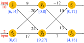
(a) Intervals

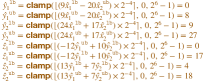
(b) Computation of intervals

Figure 3. Interval analysis on the QNN $\widehat{\mathcal{N}}_{e}$.

Figure 4. Simplified encoding of $\widehat{\mathcal{N}}_{e}$.

Example 3.7.

Consider the QNN $\widehat{\mathcal{N}}_{e}$ given in Example 2.2 with the input region $\widehat{R}_{\infty}(\hat{{\mathbf{u}}},r)$ where $\hat{{\mathbf{u}}}=(10,2)$ and $r=4$. We first get the intervals $\hat{{\mathbf{x}}}_{1}\in[6,14]$ and $\hat{{\mathbf{x}}}_{2}\in[0,6]$ for the input layer. As shown in Figure 3, we then compute the upper and lower bounds for the neurons $\hat{{\mathbf{y}}}_{1},\hat{{\mathbf{y}}}_{2}$ using the upper and lower bounds of $\hat{{\mathbf{x}}}_{1},\hat{{\mathbf{x}}}_{2}$, which are later used to compute the upper and lower bounds of the neurons $\hat{{\mathbf{z}}}_{1},\hat{{\mathbf{z}}}_{2}$. For instance, the lower bound $\hat{{\mathbf{y}}}_{1}^{\text{lb}}$ of $\hat{{\mathbf{y}}}_{1}$ is computed by the lower bound of $\hat{{\mathbf{x}}}_{1}$ and the upper bound of $\hat{{\mathbf{x}}}_{2}$ (the first equation in Figure 3(b)), because the clamp function increases monotonically, the weight between $\hat{{\mathbf{x}}}_{1}$ and $\hat{{\mathbf{y}}}_{1}$ is positive and the weight between $\hat{{\mathbf{x}}}_{2}$ and $\hat{{\mathbf{y}}}_{1}$ is negative. The other bounds are computed similarly. Based on the estimated intervals, the simplified encoding of $\widehat{\mathcal{N}}_{e}$ is shown in Figure 4, which has fewer Boolean variables and smaller constraints than the ones given in Figure 2.

4. Computing Maximum Robustness Radius

An straightforward approach to compute the maximum robustness radius (MRR) of a given input $\hat{{\mathbf{u}}}$ is to transform the problem to an optimization problem based on our encoding with an additional objective function to maximize the attack radius, and solve it directly using an ILP solver. However, this optimization problem is computationally intensive in general. As a consequence, our preliminary results show that this approach is only applicable to small-scale networks (cf. our website (Zhang et al., 2022b)).

1 Proc Main$({\tt QNN}:\widehat{\mathcal{N}},\ {\tt Input}:\hat{{\mathbf{u}}},\ {\tt StartR}:r,\ {\tt Step}:q,\ {\tt Norm}:p)$

2      if VerifyR$(\widehat{\mathcal{N}},\hat{{\mathbf{u}}},1,p)$=NonRobust then

           return $0$ ;

            // $\widehat{\mathcal{N}}$ is not robust w.r.t. $\widehat{R}_{p}(\hat{{\mathbf{u}}},1)$

3          

4           else

5                $r^{\text{lb}}$, $r^{\text{ub}}\leftarrow$ GetRange($\widehat{\mathcal{N}},\ \hat{{\mathbf{u}}},p,1,r,q$) ;

6                return GetMRR$(\widehat{\mathcal{N}},\hat{{\mathbf{u}}},p,r^{\emph{lb}},r^{\emph{ub}})$;

7               

8               

9               

10               Proc GetRange$\left(\begin{array}[]{c}{\tt QNN}:\widehat{\mathcal{N}},\ {\tt Input}:\hat{{\mathbf{u}}},\ {\tt Norm}:p,\\ {\tt MinR}:r^{\emph{lb}},\ {\tt MaxR}:r^{\emph{ub}},\ {\tt Step}:q\end{array}\right)$

11                     if VerifyR$(\widehat{\mathcal{N}},\hat{{\mathbf{u}}},r^{\emph{ub}},p)$=Robust then

12                          $r^{\text{lb}},r^{\text{ub}}\leftarrow r^{\text{ub}},r^{\text{ub}}+q$ ;

13                          return GetRange$(\widehat{\mathcal{N}},\ \hat{{\mathbf{u}}},\ p,r^{\emph{lb}},\ r^{\emph{ub}})$;

14                         

15                          return $r^{\emph{lb}}$, $r^{\emph{ub}}$;

16                         

17                          Proc GetMRR$\left(\begin{array}[]{c}{\tt QNN}:\widehat{\mathcal{N}},\ {\tt Input}:\hat{{\mathbf{u}}},\ {\tt Norm}:p,\\ {\tt MinR}:r^{\emph{lb}},\ {\tt MaxR}:r^{\emph{ub}}\end{array}\right)$

18                               if $r^{\emph{ub}}=r^{\emph{lb}}+1$ then  return $r^{\text{lb}}$ ;

19                               else

20                                    $r^{\prime}\leftarrow r^{\text{lb}}+(r^{\text{ub}}-r^{\text{lb}})//2$ ;

21                                    if VerifyR$(\widehat{\mathcal{N}},\hat{{\mathbf{u}}},r^{\prime},p)$=NonRobust then

22                                         return GetMRR$(\widehat{\mathcal{N}},\ \hat{{\mathbf{u}}},\ p,\ r^{\emph{lb}},\ r^{\prime})$;

23                                        

24                                         else  return GetMRR$(\widehat{\mathcal{N}},\ \hat{{\mathbf{u}}},\ p,\ r^{\prime},\ r^{\emph{ub}})$ ;

25                                        

26                                        

Algorithm 1 Computing MRR.

We present another approach which iteratively searches in a binary manner a potential radius $r$ for each input $\hat{{\mathbf{u}}}$ and check if the QNN is robust or not w.r.t. the input region $\widehat{R}_{p}(\hat{{\mathbf{u}}},r)$ by invoking our robustness verification procedure, named VerifyR$(\widehat{\mathcal{N}},\hat{{\mathbf{u}}},r,p)$. Our approach is described in Algorithm 1. It works as follows.

Given a QNN $\widehat{\mathcal{N}}$ and an input $\hat{{\mathbf{u}}}$, it first checks if $\widehat{\mathcal{N}}$ is robust w.r.t. $\widehat{R}_{p}(\hat{{\mathbf{u}}},1)$, i.e, the attack radius is $1$, by invoking VerifyR$(\widehat{\mathcal{N}},\hat{{\mathbf{u}}},1,p)$. If VerifyR$(\widehat{\mathcal{N}},\hat{{\mathbf{u}}},1,p)$ returns NonRobust, MRR is $0$. Otherwise, $\widehat{\mathcal{N}}$ is robust w.r.t. $\widehat{R}_{p}(\hat{{\mathbf{u}}},1)$. We then invoke the procedure GetRange to quickly determine a range $[r^{\text{lb}},r^{\text{ub}}]$ such that $\widehat{\mathcal{N}}$ is robust w.r.t. $\widehat{R}_{p}(\hat{{\mathbf{u}}},r^{\text{lb}})$ but is not robust w.r.t., $\widehat{R}_{p}(\hat{{\mathbf{u}}},r^{\text{ub}})$, where the initial value of $r^{\text{lb}}$ is $1$ and the initial value of $r^{\text{ub}}$ is $r$ provided by users. Next, it invokes the procedure GetMRR($\widehat{\mathcal{N}},\hat{{\mathbf{u}}},p,r^{\text{lb}},r^{\text{ub}}$) to search the MRR between $r^{\text{lb}}$ and $r^{\text{ub}}$ in the standard binary search manner.

The procedure GetRange receives a range $[r^{\text{lb}},r^{\text{ub}}]$ and tries to quickly update the range such that $\widehat{\mathcal{N}}$ is robust w.r.t. $\widehat{R}_{p}(\hat{{\mathbf{u}}},r^{\text{lb}})$ but is not robust w.r.t., $\widehat{R}_{p}(\hat{{\mathbf{u}}},r^{\text{ub}})$. It first checks if $\widehat{\mathcal{N}}$ is robust w.r.t. $\widehat{R}_{p}(\hat{{\mathbf{u}}},r^{\text{ub}})$. If it is the case, the range $[r^{\text{lb}},r^{\text{ub}}]$ is updated to $[r^{\text{ub}},r^{\text{ub}}+q]$ on which GetRange is recursively invoked, where $q$ is a given range size used as the search step for searching the desired range efficiently. Otherwise, the current range $[r^{\text{lb}},r^{\text{ub}}]$ is returned. We note that it is important to select an appropriate radius $r$ as the initial $r^{\text{ub}}$ and the step $q$ to compute the desired range efficiently. We remark that such a binary-search-based method can be used to find the maximum robustness radius for DNNs only if the attack radii are restricted to fixed-point values (Li et al., 2022).

5. Evaluation

We have implemented our approach as a tool QVIP, where the ILP-solver Gurobi (Gurobi, 2018) is utilized as the constraint solving engine. Gurobi does not support strict inequalities (e.g., less-than) which are used in our encoding of piecewise constant functions. To address this issue, we reformulate each integer linear constraint $g(x_{1},\cdots,x_{k})<0$ into $g(x_{1},\cdots,x_{k})+\epsilon\leq 0$ where $\epsilon>0$ is a constant smaller than the precision of $g(x_{1},\cdots,x_{k})$. For example, the integer linear constraint $(9\hat{{\mathbf{y}}}^{1}_{1}-20\hat{{\mathbf{y}}}^{1}_{2})/16<0.5v_{1}^{2,1}+\cdots+7.5v_{8}^{2,1}+\textbf{M}v_{9}^{2,1}$ of $\widehat{{\mathbf{N}}}_{e}$ (cf. Figure 4) is written as $(9\hat{{\mathbf{y}}}^{1}_{1}-20\hat{{\mathbf{y}}}^{1}_{2})/16-(0.5v_{1}^{2,1}+\cdots+7.5v_{8}^{2,1}+\textbf{M}v_{9}^{2,1})+\epsilon\leq 0$. As $\{\hat{{\mathbf{y}}}_{1}^{1},\hat{{\mathbf{y}}}_{1}^{2}\}$ and $\{v_{1}^{2,1},\ldots,v_{9}^{2,1}\}$ are integer/Boolean variables, the precision of $(9\hat{{\mathbf{y}}}^{1}_{1}-20\hat{{\mathbf{y}}}^{1}_{2})/16-(0.5v_{1}^{2,1}+\cdots+7.5v_{8}^{2,1}+\textbf{M}v_{9}^{2,1})$ is $1/16=0.0625$. Thus, $\epsilon$ can be any value s.t. $0<\epsilon<0.0625$.

Table 1. QNN benchmarks and accuracy, QNNs taken from (Henzinger et al., 2021) are marked by ${\dagger}$.

Dataset	ARCH	$Q=4$	$Q=6$	$Q=8$	$Q=10$
MNIST	P1 (784:64:10)	96.80%	97.08%†	97.10%	96.89%
MNIST	P2 (784:100:10)	97.36%	97.58%	97.45%	97.35%
MNIST	P3 (784:64:32:10)	96.91%	97.12%	97.01%	97.07%
F-MNIST	P4 (784:64:10)	–	85.60%†	–	–

We evaluate QVIP to answer the following research questions:

1. How effective is interval analysis for reducing the size of integer linear constraints and verification cost?

2. How efficient and effective is QVIP for robustness verification, compared over the state-of-the-art tools?

3. How efficient and effective is QVIP for computing MRR?

Benchmarks. We use the quantization-aware training framework provided in (Henzinger et al., 2021) to train 11 QNNs using 3 architectures, the MNIST dataset (LeCun and Cortes, 2010), and quantization configurations $\mathcal{C}_{{\mathbf{in}}}=\langle+,8,8\rangle$, $\mathcal{C}_{\mathbf{w}}=\langle\pm,Q,Q-1\rangle$, $\mathcal{C}_{\mathbf{b}}=\langle\pm,Q,Q-2\rangle$, $\mathcal{C}_{\mathbf{out}}=\langle+,Q,Q-2\rangle$ for the hidden layers and $\mathcal{C}_{\mathbf{out}}=\langle\pm,Q,Q-2\rangle$ for the output layer for a given architecture, where $Q\in\{4,6,8,10\}$. Together with 2 QNNs provided in (Henzinger et al., 2021) on which we compare with (Henzinger et al., 2021), we obtain 13 QNNs. Details of the QNNs are shown in Table 1. Column 1 gives the dataset used for training. Column 2 shows the name and architecture of the QNN, where $n_{1}:n_{2}:\cdots:n_{d}$ denotes that the QNN has $d$ layers, $n_{1}$ inputs and $n_{d}$ outputs, along with $n_{i}$ neurons in each hidden layer $\ell_{i}$ for $2\leq i\leq d-1$. Columns 3-6 list the accuracy of these QNNs. Hereafter, we denote by P$x$-$y$ the QNN using the architecture P$x$ and quantization bit size $Q=y$. We can observe that all the 12 QNNs trained on MNIST achieved more than 96.80% accuracy.

The experiments were conducted on a 28-core machine with Intel Xeon E5-2690 2.6 GHz CPU and 251 GB main memory. Note that, when using multiple threads for Gurobi, we set the number of threads to 28.

5.1. RQ1: Effectiveness of Interval Analysis

To answer RQ1, we compare the number of Boolean variables/product terms in integer linear constraints and verification time for robustness verification of the QNN P1-6 by QVIP with and without interval analysis. We randomly select 100 input samples from the test set of MNIST that can be correctly predicted by the QNN P1-6. The input regions are given by the $L_{\infty}$ norm with the attack radii $r\in\{1,2,4,6,10,20,30\}$ for each sample, resulting in 700 different input regions. We encode the robustness verification tasks of the QNN P1-6 w.r.t. all the 700 input regions with and without interval analysis, resulting a total of 1,400 verification tasks.

Attack radius $r$	1	2	4	6	10	20	30
BVar/PTerms Reduction Rate	84.6%	82.3%	76.9%	71.2%	59.6%	35.9%	22.1%
Time (with IA)	0.08	0.67	4.26	9.21	43.48	41.41	5.41
Time (without IA)	0.23	0.66	5.51	17.19	169.2	98.32	12.95

Figure 5. Results of QVIP with and without interval analysis.

The results are given in Figure 5 within 2 hours per task. The histogram shows the distribution of the tasks that can be accelerated using interval analysis, where the blue bars give the proportion of accelerated tasks among all the solved tasks, and red (resp. yellow) bars give the proportion of accelerated tasks among all the solved tasks that are robust (resp. non-robust). Note that no samples are robust under the attack radius 30. The first row in the table shows the reduction rate of the number of Boolean variables (resp. product terms) in the integer linear constraints with interval analysis and the other two rows show the average verification time (in seconds) of the solved tasks by QVIP with and without interval analysis.

Overall, we can observe that the interval analysis can drastically reduce the number of Boolean variables and product terms in the integer linear constraints, thus reduce verification cost. Unsurprisingly, we also observe that the reduction of the number of Boolean variables and product terms decreases with the increase of attack radius. It is because, with the increase of attack radius, the estimated interval becomes larger and thus the number of Boolean variables/product terms that could be reduced becomes smaller. Nevertheless, it could be quickly falsified when the attack radius is larger, thus the interval analysis is able to significantly reduce the verification cost. We note that the proportion of accelerated tasks among all the solved tasks that are robust (resp. non-robust) may increase with attack radius, i.e., red (resp. yellow) bars, but it decreases among all the solved (i.e., blue bars). It is because more and more input samples become non-robust with the increase of attack radius.

5.2. RQ2: QVIP for Robustness Verification

To answer RQ2, we first compare the performance of QVIP against the state-of-the-art verifier (smt, 2021; Henzinger et al., 2021) for robustness verification using QNNs of varied architectures but the same quantization bit size as (smt, 2021; Henzinger et al., 2021) (i.e., P1-6, P2-6, P3-6 and P4-6). We then evaluate the scalability of QVIP on the 12 MNIST QNNs, i.e., P$x$-$y$ for $x\in\{1,2,3\}$ and $y\in\{4,6,8,10\}$.

Compared with the SMT-based verifier (smt, 2021; Henzinger et al., 2021). The input regions in this comparison are completely the same as (smt, 2021; Henzinger et al., 2021):

• For P1-6 and P2-6, the attack radius $r$ is $1$ (resp. 2, 3 and 4) for the samples from the test set of MNIST with IDs 0$\sim$99 (resp. 100$\sim$199, 200$\sim$299 and 300$\sim$399). After removing all the samples that cannot be correctly predicated by P1-6, there are 99, 99, 96 and 97 samples for $r=1,2,3,4$, respectively. For P2-6, there are 98, 100, 96 and 99 samples predicted correctly.

• For P3-6, the attack radius $r$ is 1 (resp. 2, 3 and 4) for the samples from the test set of Fashion-MNIST with IDs 0$\sim$49 (resp. 100$\sim$149, 200$\sim$249 and 300$\sim$349). After removing all the samples that cannot be correctly predicated by P3-6, there are 50, 49, 48 and 49 samples for $r=1,2,3,4$, respectively.

• For P4-6, the attack radius $r$ is 1 (resp. 2, 3 and 4) for the samples from the test set of Fashion-MNIST with IDs 0$\sim$99 (resp. 100$\sim$199, 200$\sim$249 and 300$\sim$349). After removing all the samples that cannot be correctly predicated by P4-6, there are 87, 90, 43 and 44 samples for $r=1,2,3,4$, respectively.

The results are reported in Table 2. We note that the SMT-based tool only supports single-thread (smt, 2021; Henzinger et al., 2021) while our tool QVIP supports both single- and multiple-thread. Thus, we report results of QVIP in both single- and multiple-thread modes, where the multiple-thread mode uses 28 threads. Column (#S) gives the number of verification tasks for each attack radius and each QNN. Columns (SR) show the success rate of verification within 2 hours per task. Columns (Time) give the sum of verification time (in seconds) of all the solved tasks within 2 hours per task. Note that, in Columns 7 and 9, we also show the sum of verification time $(n)$ of QVIP for solving the verification tasks that are successfully solved by the SMT-based method (smt, 2021; Henzinger et al., 2021) within 2 hours per task in the single- and multiple-thread modes, respectively.

We can observe that QVIP solved significantly more verification tasks than the SMT-based method (smt, 2021; Henzinger et al., 2021) within the same time limit (2 hours) in both the single- and multiple-thread modes. In fact, QVIP solved almost all the verification tasks for P1-6 and P4-6 within 2 hours, i.e., only one verification task cannot be solved. It can be solved by neither QVIP nor the SMT-based method (smt, 2021; Henzinger et al., 2021) even using 24 hours, indicating it is a very hard problem. For the verification tasks that can be solved by the SMT-based method (smt, 2021; Henzinger et al., 2021), QVIP is two orders of magnitude faster than the state-of-the-art (smt, 2021; Henzinger et al., 2021) in both the single- and multiple-thread modes. Our conjecture is that the SMT-based method (smt, 2021; Henzinger et al., 2021) encodes the verification problem of QNNs using quantifier-free bit-vector (where the constants and bit-width are given in binary representation) and the resulting SMT constraints have a large number of If-Then-Else operations, both of which affect the runtime of the SMT-solver significantly (Henzinger et al., 2021), although interval analysis is also leveraged to reduce them. In contrast, we eliminate explicit If-Then-Else operations by introducing Boolean variables and the input/output of each neuron are encoded by integer variables. On the other hand, the decision procedures of SMT-solver and ILP-solver are completely different, indicating that the ILP-solver Gurobi is more suitable for solving constraints generated from the QNN verification problem.

We also observe that QVIP with multiple threads performs better on harder tasks, while QVIP with a single thread performs better on easier tasks. For example, considering P4-6 with $r=1$. For the 76 tasks that can be solved by SMT-based methods within 2 hours, QVIP takes 0.80 seconds using a single thread while 1.29 seconds using multiple threads. However, for the rest 11 harder tasks that cannot be solved by SMT-based method, QVIP with a single thread takes 992.6 seconds while QVIP with multiple threads only takes 48.06 seconds. In the following experiments, we use QVIP with multiple threads by default.

Table 2. QVIP vs. the SMT-based verifier (smt, 2021; Henzinger et al., 2021).

Dataset	QNN	r	#S			QVIP
				SMT-based		Single-thread		Multi-thread
				SR	Time(s)	SR	Time(s)	SR	Time(s)
		1	99	100%	14.78	100%	0.62 (0.62)	100%	1.06 (1.06)
		2	99	93.9%	3,388	100%	8.24 (1.55)	100%	10.0 (2.04)
	P1-6	3	96	72.9%	352.6	100%	210.6 (0.86)	100%	78.09 (1.47)
		4	97	54.6%	4,800	100%	779.7 (10.63)	100%	792.8 (3.22)
		1	98	83.7%	3,074	100%	80.50 (53.59)	100%	17.65 (4.27)
		2	100	22%	3,505	97%	357.9 (3.36)	97%	194.5 (5.51)
MNIST	P2-6	3	96	4.17%	417.0	94.8%	683.7 (0.25)	96.9%	1,952 (0.28)
		4	99	0%	–	80.8%	1,374 (–)	87.9%	11,166 (–)
		1	50	42%	20,383	98%	4,936 (11.49)	100%	869.9 (8.53)
		2	49	6.12%	3,759	85.7%	37,792 (38.69)	95.9%	15,699 (36.54)
	P3-6	3	48	0%	–	43.8%	26,070 (–)	50%	9,559 (–)
		4	49	0%	–	20.4%	13,735 (–)	24.5%	11,683 (–)
		1	87	87.4%	120.6	100%	993.4 (0.80)	100%	49.35 (1.29)
		2	90	81.1%	4,491	100%	838.7 (21.98)	100%	37.47 (3.19)
F-MNIST	P4-6	3	43	60.4%	4,937	100%	324.5 (1.27)	100%	99.75 (2.57)
		4	44	40.9%	136.2	97.7%	987.6 (0.43)	97.7%	138.5 (0.66)

Scalability. To understand the scalability of QVIP better, we evaluate QVIP on the 12 MNIST QNNs, i.e., P$x$-$y$ for $x\in\{1,2,3\}$ and $y\in\{4,6,8,10\}$, with larger attack radii $r\in\{2,4,6,10,20,30\}$. Following (smt, 2021; Henzinger et al., 2021), the input regions are designed as follows:

• For P1-$y$ and P2-$y$, we select 100 samples with ID varied in the interval $[(r-1)\times 100,r\times 100-1]$ from the test set of MNIST for each $r$, e.g., 100 samples with IDs $1900,\cdots,1999$ for $r=20$, where samples that cannot be correctly predicated by the QNN are removed, giving rise to at most 100 tasks for each $r$ and QNN;

• For P$3$-$y$, we select 50 samples with ID varied in the interval $[(r-1)\times 100,r\times 100-51]$ from the test set of MNIST for each $r$, where samples that cannot be correctly predicated by the QNN are removed, resulting at most 50 tasks for each $r$.

Table 3. Success rate and verification time of QVIP on MNIST dataset.

		r=2			r=4			r=6			r=10			r=20			r=30
ARCH	$Q$	#S	SR	Time	#S	SR	Time	#S	SR	Time	#S	SR	Time	#S	SR	Time	#S	SR	Time
	4	97	100%	25.35	96	100%	34.68	97	90.7%	165.4	94	94.7%	345.9	97	99.0%	53.21	95	100%	2.66
	6	99	100%	0.10	97	100%	8.17	97	96.9%	12.60	97	94.8%	204.0	95	95.8%	60.83	93	100%	9.40
P1	8	100	100%	0.02	97	100%	0.08	97	100%	0.23	96	100%	0.54	97	100%	0.82	96	87.65%	90.47
	10	99	100%	0.02	98	100%	0.11	96	100%	0.35	95	100%	0.92	93	100%	1.62	93	100%	21.59
	4	99	100%	17.3	98	95.9%	229.4	97	72.2%	379.0	96	64.9%	575.9	95	96.8%	276.3	96	100%	28.96
	6	100	97%	2.00	99	87.9%	128.3	100	61%	282.8	94	27.6%	1,107	96	68.8%	574.4	96	91.7%	221.6
P2	8	99	100%	0.04	98	100%	0.26	99	100%	0.48	95	100%	0.79	93	100%	3.88	95	62.1%	143.6
	10	99	100%	0.03	97	100%	0.28	97	100%	0.63	96	100%	1.13	97	100%	1.77	96	91.7%	31.50
	4	50	100%	277.1	49	44.9%	348.4	50	26%	1,406	49	32.7%	1,546	48	75%	1,252	46	89.1%	549.9
	6	49	95.9%	334.0	49	24.5%	973.6	50	4%	3,658	49	10.2%	1,137	47	29.8%	1,510	47	74.5%	951.5
P3	8	48	100%	0.27	47	100%	0.45	50	100%	0.51	48	100%	2.99	46	100%	43.61	47	74.5%	513.0
	10	49	100%	0.55	47	100%	0.94	50	100%	1.13	49	100%	1.57	48	100%	345.7	47	100%	568.6

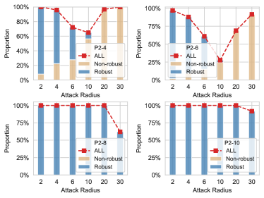
Figure 6. Distribution of (non-)robust samples under various attack radii $r$ and quantization bits $Q$.

Table 3 shows the results of QVIP within 2 hours per task, where columns (#S), (SR) and (Time) respectively give the number of verification tasks for each attack radius and each QNN, the success rate of verification, and average verification time of all the solved tasks. Overall, the results show that QVIP scales to larger QNNs with the attack radius $r$ up to 30.

Interestingly, we found that the verification cost is non-monotonic w.r.t. the attack radius. To understand the reason, we analyze the distribution of (non-)robust samples that are solved by QVIP. The results on the QNNs P2-$y$ for $y\in\{4,6,8,10\}$ for each attack radius $r$ are shown in Figure 6. The blue (resp. yellow) bars show the proportion (in percentage) of robust (resp. non-robust) samples among all the solved tasks. The red dotted line reflects the change in the verification success rate. From the upper two sub-figures in Figure 6, we can observe that the success rate falls when the attack radius closing the robustness boundary and rises afterwards, conforming to the non-monotonicity in verification cost in Table 3. This indicates that the robustness of QNNs w.r.t. input regions with smaller or larger attack radii $r$ is relatively easier to prove/falsify, while it is harder for the attack radii close to the robustness boundary. We also found that though the accuracy of these QNNs are similar (cf. Table 1), their robustness are quite different, and particularly using more quantization bits results in an overall more robust QNN, i.e., more robust samples under the same attack radius. Similar results can be observed for P1-$y$ and P3-$y$ (cf. our website (Zhang et al., 2022b)).

5.3. RQ3: QVIP for Computing MRR

To answer RQ3, we use QVIP to compute the maximum robustness radii for QNNs P1-4 and P1-6. We use the same 100 samples of MNIST as in Section 5.1, resulting in 200 computation tasks in total. Each task is run by QVIP with 2 hours timeout. Recall that it is essential to select appropriate values for StartR and Step parameters of Algorithm 1. In this work, we conduct the experiments only to demonstrate the feasibility of QVIP on MRR computation, hence we set the two parameters both as 10 directly.

QVIP successfully solved 68 of the 100 computation tasks for P1-6 with an average of 1,042 seconds per task, and solved 59 of the 100 computation tasks for P1-4 with an average of 1,007 seconds per task. Figure 7 shows the MRR distribution of the solved tasks on two QNNs. We can observe that the MRR distribution of P1-4 is more intensive with the average value 5 than the one of P1-6 with the average value 9.

The overall MRR of QNNs w.r.t. the same given set of samples also allow us to quantitatively measure and compare the robustness of QNNs. From the results, we can observe that P1-6 is more robust than P1-4 over the given set of 100 samples w.r.t. the distribution as well as the average MRR. We note that the comparison result would be more convincing by increasing the number of samples as well as their diversity.

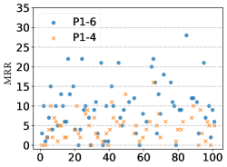
Figure 7. Distribution of maximum robustness radii.

5.4. Threats to Validity

Our approach is designed for verifying quantized neural networks typically deployed in safety-critical resource-constrained devices, where the number of quantization bits and neurons is not large. In this context, the completeness of the approach is significant. However, large-scale neural networks in different application domains may require abstraction techniques, at the cost of completeness. In this work, we focus on quantized feed-forward ReLU networks, one of the most fundamental and common architectures. It requires more experiments to confirm whether our approach still outperforms the SMT-based method for other quantized neural networks. Below, we discuss potential external and internal threats to the validity of our results.

One of the potential external threats is the selection of evaluation subjects. To mitigate this threat, we use 13 QNNs with the same or similar architectures as (Giacobbe et al., 2020; Henzinger et al., 2021), trained on two datasets, MNIST and Fashion-MNIST, both of which are widely used for training QNNs/BNNs in the literature, e.g., (Narodytska et al., 2018; Baluta et al., 2019; Amir et al., 2020; Henzinger et al., 2021; Zhang et al., 2021; Giacobbe et al., 2020). To be diverse, the QNNs involve 3 architectures and 4 quantization bit sizes, and the attack radius is set in a wide range (e.g., from 1 to 30 for QNNs trained on MNIST).

Another potential external threat is that the solving time of two ILP problems with similar sizes can be quite different. Consequently, the verification time of the same QNN and same attack radius for different samples can be quite different. To mitigate this threat, for each QNN and each attack radius, we evaluate our tool QVIP on 50$\sim$100 samples, showing that QVIP performs well on most cases, and significantly outperforms the state-of-the-art verifier (smt, 2021; Henzinger et al., 2021).

The internal threat mainly comes from the interval analysis strategy used to reduce the size of constraints and verification cost while there is no theoretical guarantee. To mitigate this threat, we analyze the reduction of the number of Boolean variables and product terms in the encodings of the QNN P1-6 using 100 input samples with attack radius from 2 to 30, resulting in 1400 encodings in total. The results show that interval analysis is very effective in most cases. While the effectiveness of reducing the number of Boolean variables and product terms decreases with the increases of the attack radius, the verification cost can still be reduced significantly.

6. Related Work

There is a large and growing body of work on quality assurance techniques for (quantized) DNNs including testing (e.g., (Carlini and Wagner, 2017; Ma et al., 2018a, b; Pei et al., 2017; Sun et al., 2018; Tian et al., 2018; Xie et al., 2019a; Shumailov et al., 2019; Odena et al., 2019; Xie et al., 2019b; Baluta et al., 2021; Webb et al., 2019; Zhang et al., 2022a; Zhao et al., 2021)) and formal verification (e.g.,  (Pulina and Tacchella, 2010; Ehlers, 2017; Katz et al., 2017, 2019; Gehr et al., 2018; Huang et al., 2017; Singh et al., 2019b; Wang et al., 2018; Tran et al., 2019; Gokulanathan et al., 2020; Ashok et al., 2020; Elboher et al., 2020; Yang et al., 2021; Liu et al., 2020; Guo et al., 2021; Zhao et al., 2022; Liu et al., 2022)). While testing techniques are often effective in finding violations of properties, they cannot prove their absence; formal verification and testing are normally complementary. In this section, we mainly discuss the existing formal verification techniques for (quantized) DNNs, which are classified into the following categories: constraint solving based, abstraction based, and decision diagram based.

Constraint solving based methods. Early work on formal verification of real numbered DNNs typically reduces the problem to the solving of Satisfiability Modulo Theory (SMT) problem (Katz et al., 2017, 2019; Pulina and Tacchella, 2010) or Mixed Integer Linear Programming (MILP) problem (Cheng et al., 2017; Dutta et al., 2017; Fischetti and Jo, 2018), that can be solved by off-the-shelf or dedicated solvers. In theory, such techniques are both sound and complete unless abstraction techniques are adopted to improve scalability. However, verification tools for real numbered DNNs cannot be used to guarantee the robustness of quantized DNNs (i.e., QNNs) due to the fixed-point semantics of QNNs (Giacobbe et al., 2020).

Along this line, Narodytska et al. (Narodytska et al., 2018) proposed to reduce the verification problem of 1-bit quantized DNNs (i.e., BNNs) to the satisfiability problem of Boolean formulas (SAT) or the solving of integer linear constraints. Our QNN encoding can be seen as a non-trivial generalization of their BNN encoding (Narodytska et al., 2018). Furthermore, we also propose to leverage interval analysis to effectively reduce the size of constraints and verification cost. Using a similar encoding of (Narodytska et al., 2018), Baluta et al. proposed a PAC-style quantitative analysis framework for BNNs (Baluta et al., 2019) by leveraging approximate SAT model-counting solvers. Jia and Rinard extended the encoding to three-valued BNNs (Jia and Rinard, 2020). Narodytska et al. proposed a SAT-based verification-friendly BNN training framework (Narodytska et al., 2020).

Recently, accounting for the fixed-point semantics of QNNs, Giacobbe et al. (Giacobbe et al., 2020) pushed this direction further by introducing the first formal verification approach for multiple-bit quantized DNNs (i.e., QNNs). They encode the verification problem of QNNs in first-order theory of quantifier-free bit-vector with binary representation. Later, first-order theory of fixed-point was proposed and used to verify QNNs (Baranowski et al., 2020). Henzinger et al. (Henzinger et al., 2021) explored several heuristics to improve efficiency and scalability of the SMT-based approach (Giacobbe et al., 2020). To the best our knowledge, we are the first to reduce the verification problem of QNNs to the solving of integer linear constraints. Experimental results show that our approach is significantly faster than the state-of-the-art (Henzinger et al., 2021).

Abstraction based methods. To improve efficiency and scalability, various abstraction techniques have been used, which typically compute conservative bounds on the value ranges of the neurons for an input region of interest. Abstract interpretation (Cousot and Cousot, 1977) has been widely used by exploring networks layer by layer (Anderson et al., 2019; Gehr et al., 2018; Li et al., 2019, 2020; Singh et al., 2019a, 2018; Wang et al., 2018; Singh et al., 2019b; Tran et al., 2020, 2019; Yang et al., 2021), typically with different abstract domains. Almost all the existing work considered real numbered DNNs while few work (e.g., (Singh et al., 2019b)) considered floating-point numbered DNNs. The interval analysis adopted in this work is an application of abstract interpretation with interval as its abstract domain. It is an interesting future work to study other abstract interpretation based techniques to reduce the size of integer linear constraints. Another direction is to abstract neural networks (Ashok et al., 2020; Elboher et al., 2020; Ostrovsky et al., 2022), rendering them suitable for formal verification. Abstraction based methods are sound but incomplete, so refinement techniques are normally needed to tighten bounds or refine over-simplified networks.

While widely used for verifying DNNs, abstraction based verification of both QNNs and BNNs is very limited, except for the work (Henzinger et al., 2021) which, similar to ours, is used to reduce the size of SMT formulas and verification cost.

Differential verification (Lahiri et al., 2013) initially proposed for verifying a new version of a program w.r.t. a previous version, has been applied to QNNs (Paulsen et al., 2020a, b; Mohammadinejad et al., 2021). In general, they check if two (quantified) DNNs with the same architecture but different parameters output similar results (e.g., bounded by a small value) for each input from an input region. As mentioned previously, these techniques cannot be used to directly and precisely verify the robustness of QNNs.

Decision diagram based methods. Decision diagram based verification methods were proposed for behavior analysis and verification of BNNs (Choi et al., 2019; Shih et al., 2019b, a; Zhang et al., 2021), e.g., allowing one to reason about the distribution of the adversarial examples or give an interpretation on the decision made by a BNN. Choi et al. (Choi et al., 2019) proposed a knowledge compilation based encoding that first transforms a BNN into a tractable Boolean circuit and then into a more tractable circuit, called Sentential Decision Diagram (SDD). Based on the SDD representation, polynomial-time queries to SDD can be utilized to explain and verify the behaviors of BNNs efficiently. In parallel, Shih et al. proposed a quantitative verification framework for BNNs (Shih et al., 2019b, a), where a given BNN with an input region of interest is modeled using a Binary Decision Diagram (BDD) by leveraging BDD-learning (Nakamura, 2005), which has limited scalability. Very recently, Zhang et al. (Zhang et al., 2021) proposed a novel BDD-based verification framework for BNNs, which exploits the internal structure of the BNNs to construct BDD models instead of BDD-learning. Specifically, they translated the input-output relation of blocks in BNNs to cardinality constraints which can then be encoded by BDDs. Though decision diagram based methods enable behavior analysis and quantitative verification, they can hardly be extended to QNNs, i.e., multiple-bit quantized DNNs, due to the large space of QNNs.

7. Conclusion

We have proposed the first ILP-based analysis approach for QNNs. We presented a prototype tool QVIP and conducted thorough experiments on various QNNs with different quantization bit sizes. Experimental results showed that QVIP is more efficient and scalable than the state-of-the-art, enabling the computation of maximum robustness radii for QNNs which can be used as a metric for robustness evaluation of QNNs. We also found that the accuracy of QNNs stays similar under different quantization bits, but the robustness can be greatly improved with more quantization bits, using quantization-aware training while it is not using post-training quantization.

This work presented the first step towards the formal verification of QNNs. For future work, it would be interesting to investigate formal verification of QNNs that have more complicated architectures, activation functions, and a larger number of neurons.

- (1)
- smt (2021) 2021. Scalable Verification of Quantized Neural Networks. https://github.com/mlech26l/qnn_robustness_benchmarks.
- TFL (2022) 2022. Tensorflow Lite. https://www.tensorflow.org/lite.
- Amir et al. (2020) Guy Amir, Haoze Wu, Clark W. Barrett, and Guy Katz. 2020. An SMT-Based Approach for Verifying Binarized Neural Networks. CoRR abs/2011.02948 (2020).
- Anderson et al. (2019) Greg Anderson, Shankara Pailoor, Isil Dillig, and Swarat Chaudhuri. 2019. Optimization and abstraction: a synergistic approach for analyzing neural network robustness. In Proceedings of the 40th ACM SIGPLAN Conference on Programming Language Design and Implementation. 731–744.
- Apollo (2018) Apollo. 2018. An open, reliable and secure software platform for autonomous driving systems. http://apollo.auto.
- Ashok et al. (2020) Pranav Ashok, Vahid Hashemi, Jan Kretínský, and Stefanie Mohr. 2020. DeepAbstract: Neural Network Abstraction for Accelerating Verification. In Proceedings of the 18th International Symposium on Automated Technology for Verification and Analysis. 92–107.
- Baluta et al. (2021) Teodora Baluta, Zheng Leong Chua, Kuldeep S Meel, and Prateek Saxena. 2021. Scalable quantitative verification for deep neural networks. In 2021 IEEE/ACM 43rd International Conference on Software Engineering. IEEE, 312–323.
- Baluta et al. (2019) Teodora Baluta, Shiqi Shen, Shweta Shinde, Kuldeep S Meel, and Prateek Saxena. 2019. Quantitative verification of neural networks and its security applications. In Proceedings of the 2019 ACM SIGSAC Conference on Computer and Communications Security. 1249–1264.
- Baranowski et al. (2020) Marek S. Baranowski, Shaobo He, Mathias Lechner, Thanh Son Nguyen, and Zvonimir Rakamaric. 2020. An SMT Theory of Fixed-Point Arithmetic. In Proceedings of the 10th International Joint Conference on Automated Reasoning. 13–31.
- Bu et al. (2021) Lei Bu, Zhe Zhao, Yuchao Duan, and Fu Song. 2021. Taking Care of The Discretization Problem: A Comprehensive Study of the Discretization Problem and A Black-Box Adversarial Attack in Discrete Integer Domain. IEEE Transactions on Dependable and Secure Computing (2021), 1–18. https://doi.org/10.1109/TDSC.2021.3088661
- Carlini and Wagner (2017) Nicholas Carlini and David A. Wagner. 2017. Towards Evaluating the Robustness of Neural Networks. In Proceedings of the 2017 IEEE Symposium on Security and Privacy. 39–57.
- Chen et al. (2021a) Guangke Chen, Sen Chen, Lingling Fan, Xiaoning Du, Zhe Zhao, Fu Song, and Yang Liu. 2021a. Who is Real Bob? Adversarial Attacks on Speaker Recognition Systems. In Proceedings of the 42nd IEEE Symposium on Security and Privacy. 694–711.
- Chen et al. (2021b) Guangke Chen, Zhe Zhao, Fu Song, Sen Chen, Lingling Fan, and Yang Liu. 2021b. SEC4SR: a security analysis platform for speaker recognition. arXiv preprint arXiv:2109.01766 (2021).
- Chen et al. (2022a) Guangke Chen, Zhe Zhao, Fu Song, Sen Chen, Lingling Fan, and Yang Liu. 2022a. AS2T: Arbitrary Source-To-Target Adversarial Attack on Speaker Recognition Systems. IEEE Transactions on Dependable and Secure Computing (2022), 1–17. https://doi.org/10.1109/TDSC.2022.3189397
- Chen et al. (2022b) Guangke Chen, Zhe Zhao, Fu Song, Sen Chen, Lingling Fan, Feng Wang, and Jiashui Wang. 2022b. Towards Understanding and Mitigating Audio Adversarial Examples for Speaker Recognition. arXiv preprint arXiv:2206.03393 (2022).
- Cheng et al. (2017) Chih-Hong Cheng, Georg Nührenberg, and Harald Ruess. 2017. Maximum Resilience of Artificial Neural Networks. In Proceedings of the 15th International Symposium on Automated Technology for Verification and Analysis (ATVA). 251–268.
- Choi et al. (2019) Arthur Choi, Weijia Shi, Andy Shih, and Adnan Darwiche. 2019. Compiling Neural Networks into Tractable Boolean Circuits. In Proceedings of the AAAI Spring Symposium on Verification of Neural Networks.
- Ciresan et al. (2012) Dan C. Ciresan, Alessandro Giusti, Luca Maria Gambardella, and Jürgen Schmidhuber. 2012. Deep Neural Networks Segment Neuronal Membranes in Electron Microscopy Images. In Proceedings of Annual Conference on Neural Information Processing Systems. 2852–2860.
- Cousot and Cousot (1977) Patrick Cousot and Radhia Cousot. 1977. Abstract Interpretation: A Unified Lattice Model for Static Analysis of Programs by Construction or Approximation of Fixpoints. In Conference Record of the Fourth ACM Symposium on Principles of Programming Languages. 238–252.
- Dutta et al. (2017) Souradeep Dutta, Susmit Jha, Sriram Sanakaranarayanan, and Ashish Tiwari. 2017. Output range analysis for deep neural networks. arXiv preprint arXiv:1709.09130 (2017).
- Ehlers (2017) Rüdiger Ehlers. 2017. Formal Verification of Piece-Wise Linear Feed-Forward Neural Networks. In Proceedings of the 15th International Symposium on Automated Technology for Verification and Analysis. 269–286.
- Elboher et al. (2020) Yizhak Yisrael Elboher, Justin Gottschlich, and Guy Katz. 2020. An Abstraction-Based Framework for Neural Network Verification. In Proceedings of the 32nd International Conference on Computer Aided Verification. 43–65.
- Eykholt et al. (2018) Kevin Eykholt, Ivan Evtimov, Earlence Fernandes, Bo Li, Amir Rahmati, Chaowei Xiao, Atul Prakash, Tadayoshi Kohno, and Dawn Song. 2018. Robust Physical-World Attacks on Deep Learning Visual Classification. In Proceedings of 2018 IEEE Conference on Computer Vision and Pattern Recognition. 1625–1634.
- Fischetti and Jo (2018) Matteo Fischetti and Jason Jo. 2018. Deep neural networks and mixed integer linear optimization. Constraints 23, 3 (2018), 296–309.
- Gehr et al. (2018) Timon Gehr, Matthew Mirman, Dana Drachsler-Cohen, Petar Tsankov, Swarat Chaudhuri, and Martin T. Vechev. 2018. AI2: Safety and Robustness Certification of Neural Networks with Abstract Interpretation. In Proceedings of the 2018 IEEE Symposium on Security and Privacy. 3–18.
- Giacobbe et al. (2020) Mirco Giacobbe, Thomas A. Henzinger, and Mathias Lechner. 2020. How Many Bits Does it Take to Quantize Your Neural Network?. In Proceedings of the 26th International Conference on Tools and Algorithms for the Construction and Analysis of Systems. 79–97.
- Gokulanathan et al. (2020) Sumathi Gokulanathan, Alexander Feldsher, Adi Malca, Clark W. Barrett, and Guy Katz. 2020. Simplifying Neural Networks Using Formal Verification. In Proceedings of the 12th International Symposium NASA Formal Methods. 85–93.
- Goodfellow et al. (2015) Ian Goodfellow, Jonathon Shlens, and Christian Szegedy. 2015. Explaining and harnessing adversarial examples. In Proceedings of the 3th International Conference on Learning Representations.
- Guo et al. (2021) Xingwu Guo, Wenjie Wan, Zhaodi Zhang, Min Zhang, Fu Song, and Xuejun Wen. 2021. Eager Falsification for Accelerating Robustness Verification of Deep Neural Networks. In Proceedings of the 32nd IEEE International Symposium on Software Reliability Engineering. 345–356.
- Gurobi (2018) Gurobi. 2018. A most powerful mathematical optimization solver. https://www.gurobi.com/.
- Han et al. (2016) Song Han, Huizi Mao, and William J. Dally. 2016. Deep Compression: Compressing Deep Neural Network with Pruning, Trained Quantization and Huffman Coding. In Proceedings of the 4th International Conference on Learning Representations.
- Henzinger et al. (2021) Thomas A. Henzinger, Mathias Lechner, and Dorde Zikelic. 2021. Scalable Verification of Quantized Neural Networks. In Proceedings of the 35th Conference on Artificial Intelligence, the 33th Conference on Innovative Applications of Artificial Intelligence, the 11th Symposium on Educational Advances in Artificial Intelligence. 3787–3795.
- Hinton et al. (2012) G. Hinton, L. Deng, D. Yu, G. E. Dahl, A. Mohamed, N. Jaitly, A. Senior, V. Vanhoucke, P. Nguyen, T. N. Sainath, and B. Kingsbury. 2012. Deep Neural Networks for Acoustic Modeling in Speech Recognition: The Shared Views of Four Research Groups. IEEE Signal Process. Mag. 29, 6 (2012), 82–97.
- Huang et al. (2017) Xiaowei Huang, Marta Kwiatkowska, Sen Wang, and Min Wu. 2017. Safety Verification of Deep Neural Networks. In Proceedings of the 29th International Conference on Computer Aided Verification. 3–29.
- Jacob et al. (2018) Benoit Jacob, Skirmantas Kligys, Bo Chen, Menglong Zhu, Matthew Tang, Andrew G. Howard, Hartwig Adam, and Dmitry Kalenichenko. 2018. Quantization and Training of Neural Networks for Efficient Integer-Arithmetic-Only Inference. In Proceedings of the IEEE Conference on Computer Vision and Pattern Recognition. 2704–2713.
- Jia and Rinard (2020) Kai Jia and Martin Rinard. 2020. Efficient Exact Verification of Binarized Neural Networks. In Proceedings of the Annual Conference on Neural Information Processing Systems.
- Karpathy et al. (2014) Andrej Karpathy, George Toderici, Sanketh Shetty, Thomas Leung, Rahul Sukthankar, and Fei-Fei Li. 2014. Large-Scale Video Classification with Convolutional Neural Networks. In Proceedings of 2014 IEEE Conference on Computer Vision and Pattern Recognition. 1725–1732.
- Katz et al. (2017) Guy Katz, Clark W. Barrett, David L. Dill, Kyle Julian, and Mykel J. Kochenderfer. 2017. Reluplex: An Efficient SMT Solver for Verifying Deep Neural Networks. In Proceedings of the 29th International Conference on Computer Aided Verification. 97–117.
- Katz et al. (2019) Guy Katz, Derek A. Huang, Duligur Ibeling, Kyle Julian, Christopher Lazarus, Rachel Lim, Parth Shah, Shantanu Thakoor, Haoze Wu, Aleksandar Zeljic, David L. Dill, Mykel J. Kochenderfer, and Clark W. Barrett. 2019. The Marabou Framework for Verification and Analysis of Deep Neural Networks. In Proceedings of the 31st International Conference on Computer Aided Verification. 443–452.
- Kurakin et al. (2017) Alexey Kurakin, Ian Goodfellow, and Samy Bengio. 2017. Adversarial examples in the physical world. In Proceedings of International Conference on Learning Representations.
- Lahiri et al. (2013) Shuvendu K. Lahiri, Kenneth L. McMillan, Rahul Sharma, and Chris Hawblitzel. 2013. Differential assertion checking. In Proceedings of the Joint Meeting of the European Software Engineering Conference and the ACM SIGSOFT Symposium on the Foundations of Software Engineering. 345–355.
- LeCun and Cortes (2010) Yann LeCun and Corinna Cortes. 2010. MNIST handwritten digit database.
- Li et al. (2019) Jianlin Li, Jiangchao Liu, Pengfei Yang, Liqian Chen, Xiaowei Huang, and Lijun Zhang. 2019. Analyzing Deep Neural Networks with Symbolic Propagation: Towards Higher Precision and Faster Verification. In Proceedings of the 26th International Symposium on Static Analysis. 296–319.
- Li et al. (2020) Renjue Li, Jianlin Li, Cheng-Chao Huang, Pengfei Yang, Xiaowei Huang, Lijun Zhang, Bai Xue, and Holger Hermanns. 2020. PRODeep: a platform for robustness verification of deep neural networks. In Proceedings of the 28th ACM Joint European Software Engineering Conference and Symposium on the Foundations of Software Engineering. 1630–1634.
- Li et al. (2022) Renjue Li, Pengfei Yang, Cheng-Chao Huang, Youcheng Sun, Bai Xue, and Lijun Zhang. 2022. Towards practical robustness analysis for DNNs based on PAC-model learning. In Proceedings of the IEEE/ACM 44th International Conference on Software Engineering. 2189–2201.
- Liu et al. (2022) Jiaxiang Liu, Yunhan Xing, Xiaomu Shi, Fu Song, Zhiwu Xu, and Zhong Ming. 2022. Abstraction and Refinement: Towards Scalable and Exact Verification of Neural Networks. CoRR abs/2207.00759 (2022).
- Liu et al. (2020) Wan-Wei Liu, Fu Song, Tang-Hao-Ran Zhang, and Ji Wang. 2020. Verifying ReLU Neural Networks from a Model Checking Perspective. J. Comput. Sci. Technol. 35, 6 (2020), 1365–1381.
- Ma et al. (2018a) Lei Ma, Felix Juefei-Xu, Fuyuan Zhang, Jiyuan Sun, Minhui Xue, Bo Li, Chunyang Chen, Ting Su, Li Li, Yang Liu, Jianjun Zhao, and Yadong Wang. 2018a. DeepGauge: multi-granularity testing criteria for deep learning systems. In Proceedings of the 33rd ACM/IEEE International Conference on Automated Software Engineering. 120–131.
- Ma et al. (2018b) Shiqing Ma, Yingqi Liu, Wen-Chuan Lee, Xiangyu Zhang, and Ananth Grama. 2018b. MODE: automated neural network model debugging via state differential analysis and input selection. In Proceedings of the 2018 ACM Joint Meeting on European Software Engineering Conference and Symposium on the Foundations of Software Engineering. 175–186.
- Mohammadinejad et al. (2021) Sara Mohammadinejad, Brandon Paulsen, Jyotirmoy V. Deshmukh, and Chao Wang. 2021. DiffRNN: Differential Verification of Recurrent Neural Networks. In Proceedings of the 19th International Conference on Formal Modeling and Analysis of Timed Systems. 117–134.
- Moore et al. (2009) Ramon E Moore, R Baker Kearfott, and Michael J Cloud. 2009. Introduction to interval analysis. Vol. 110. Siam.
- Nagel et al. (2021) Markus Nagel, Marios Fournarakis, Rana Ali Amjad, Yelysei Bondarenko, Mart van Baalen, and Tijmen Blankevoort. 2021. A white paper on neural network quantization. arXiv preprint arXiv:2106.08295 (2021).
- Nakamura (2005) Atsuyoshi Nakamura. 2005. An efficient query learning algorithm for ordered binary decision diagrams. Inf. Comput. 201, 2 (2005), 178–198.
- Narodytska et al. (2018) Nina Narodytska, Shiva Prasad Kasiviswanathan, Leonid Ryzhyk, Mooly Sagiv, and Toby Walsh. 2018. Verifying Properties of Binarized Deep Neural Networks. In Proceedings of the AAAI Conference on Artificial Intelligence. 6615–6624.
- Narodytska et al. (2020) Nina Narodytska, Hongce Zhang, Aarti Gupta, and Toby Walsh. 2020. In Search for a SAT-friendly Binarized Neural Network Architecture. In Proceedings of the 8th International Conference on Learning Representations.
- Odena et al. (2019) Augustus Odena, Catherine Olsson, David G. Andersen, and Ian J. Goodfellow. 2019. TensorFuzz: Debugging Neural Networks with Coverage-Guided Fuzzing. In Proceedings of the 36th International Conference on Machine Learning. 4901–4911.
- Ostrovsky et al. (2022) Matan Ostrovsky, Clark W. Barrett, and Guy Katz. 2022. An Abstraction-Refinement Approach to Verifying Convolutional Neural Networks. CoRR abs/2201.01978 (2022).
- Papernot et al. (2016) Nicolas Papernot, Patrick D. McDaniel, Somesh Jha, Matt Fredrikson, Z. Berkay Celik, and Ananthram Swami. 2016. The Limitations of Deep Learning in Adversarial Settings. In Proceedings of IEEE European Symposium on Security and Privacy. 372–387.
- Paulsen et al. (2020a) Brandon Paulsen, Jingbo Wang, and Chao Wang. 2020a. ReluDiff: differential verification of deep neural networks. In Proceedings of the 42nd International Conference on Software Engineering. 714–726.
- Paulsen et al. (2020b) Brandon Paulsen, Jingbo Wang, Jiawei Wang, and Chao Wang. 2020b. NeuroDiff: Scalable Differential Verification of Neural Networks using Fine-Grained Approximation. In Proceedings of the 35th IEEE/ACM International Conference on Automated Software Engineering. 784–796.
- Pei et al. (2017) Kexin Pei, Yinzhi Cao, Junfeng Yang, and Suman Jana. 2017. DeepXplore: Automated Whitebox Testing of Deep Learning Systems. In Proceedings of the 26th Symposium on Operating Systems Principles. 1–18.
- Pennington et al. (2014) Jeffrey Pennington, Richard Socher, and Christopher D. Manning. 2014. Glove: Global Vectors for Word Representation. In Proceedings of the 2014 Conference on Empirical Methods in Natural Language Processing. 1532–1543.
- Pulina and Tacchella (2010) Luca Pulina and Armando Tacchella. 2010. An Abstraction-Refinement Approach to Verification of Artificial Neural Networks. In Proceedings of the 22nd International Conference on Computer Aided Verification. 243–257.
- Shih et al. (2019a) Andy Shih, Adnan Darwiche, and Arthur Choi. 2019a. Verifying binarized neural networks by angluin-style learning. In Proceedings of the 2019 International Conference on Theory and Applications of Satisfiability Testing. 354–370.
- Shih et al. (2019b) Andy Shih, Adnan Darwiche, and Arthur Choi. 2019b. Verifying binarized neural networks by local automaton learning. In Proceedings of the AAAI Spring Symposium on Verification of Neural Networks.
- Shumailov et al. (2019) Ilia Shumailov, Yiren Zhao, Robert Mullins, and Ross Anderson. 2019. To compress or not to compress: Understanding the interactions between adversarial attacks and neural network compression. Proceedings of Machine Learning and Systems 1 (2019), 230–240.
- Singh et al. (2019a) Gagandeep Singh, Rupanshu Ganvir, Markus Püschel, and Martin T. Vechev. 2019a. Beyond the Single Neuron Convex Barrier for Neural Network Certification. In Proceedings of the Annual Conference on Neural Information Processing Systems. 15072–15083.
- Singh et al. (2018) Gagandeep Singh, Timon Gehr, Matthew Mirman, Markus Püschel, and Martin T. Vechev. 2018. Fast and Effective Robustness Certification. In Proceedings of the Annual Conference on Neural Information Processing Systems. 10825–10836.
- Singh et al. (2019b) Gagandeep Singh, Timon Gehr, Markus Püschel, and Martin T. Vechev. 2019b. An abstract domain for certifying neural networks. Proceedings of the ACM on Programming Languages (POPL) 3 (2019), 41:1–41:30.
- Song et al. (2021) Fu Song, Yusi Lei, Sen Chen, Lingling Fan, and Yang Liu. 2021. Advanced evasion attacks and mitigations on practical ML-based phishing website classifiers. Int. J. Intell. Syst. 36, 9 (2021), 5210–5240.
- Sun et al. (2018) Youcheng Sun, Min Wu, Wenjie Ruan, Xiaowei Huang, Marta Kwiatkowska, and Daniel Kroening. 2018. Concolic testing for deep neural networks. In Proceedings of the 33rd ACM/IEEE International Conference on Automated Software Engineering. 109–119.
- Szegedy et al. (2014) Christian Szegedy, Wojciech Zaremba, Ilya Sutskever, Joan Bruna, Dumitru Erhan, Ian Goodfellow, and Rob Fergus. 2014. Intriguing properties of neural networks. In Proceedings of International Conference on Learning Representations.
- Tan and Le (2019) Mingxing Tan and Quoc V. Le. 2019. EfficientNet: Rethinking Model Scaling for Convolutional Neural Networks. In Proceedings of the 36th International Conference on Machine Learning. 6105–6114.
- Tian et al. (2018) Yuchi Tian, Kexin Pei, Suman Jana, and Baishakhi Ray. 2018. DeepTest: automated testing of deep-neural-network-driven autonomous cars. In Proceedings of the 40th International Conference on Software Engineering. 303–314.
- Tjeng et al. (2019) Vincent Tjeng, Kai Xiao, and Russ Tedrake. 2019. Evaluating Robustness Of Neural Networks With Mixed Integer Programming. In Proceedings of the 7th International Conference on Learning Representations.
- Tran et al. (2020) Hoang-Dung Tran, Stanley Bak, Weiming Xiang, and Taylor T. Johnson. 2020. Verification of Deep Convolutional Neural Networks Using ImageStars. In Proceedings of the International Conference on Computer Aided Verification. 18–42.
- Tran et al. (2019) Hoang-Dung Tran, Diego Manzanas Lopez, Patrick Musau, Xiaodong Yang, Luan Viet Nguyen, Weiming Xiang, and Taylor T. Johnson. 2019. Star-Based Reachability Analysis of Deep Neural Networks. In Proceedings of the 3rd World Congress on Formal Methods. 670–686.
- Wang et al. (2018) Shiqi Wang, Kexin Pei, Justin Whitehouse, Junfeng Yang, and Suman Jana. 2018. Formal Security Analysis of Neural Networks using Symbolic Intervals. In Proceedings of the 27th USENIX Security Symposium. 1599–1614.
- Webb et al. (2019) Stefan Webb, Tom Rainforth, Yee Whye Teh, and M. Pawan Kumar. 2019. A Statistical Approach to Assessing Neural Network Robustness. In Proceedings of the 7th International Conference on Learning Representations.
- WikiChip (2022) WikiChip. Accessed April 30, 2022. FSD Chip - Tesla. https://en.wikichip.org/wiki/tesla_(car_company)/fsd_chip.
- Xiao et al. (2017) Han Xiao, Kashif Rasul, and Roland Vollgraf. 2017. Fashion-MNIST: a Novel Image Dataset for Benchmarking Machine Learning Algorithms. CoRR abs/1708.07747 (2017).
- Xie et al. (2019a) Xiaofei Xie, Lei Ma, Felix Juefei-Xu, Minhui Xue, Hongxu Chen, Yang Liu, Jianjun Zhao, Bo Li, Jianxiong Yin, and Simon See. 2019a. DeepHunter: a coverage-guided fuzz testing framework for deep neural networks. In Proceedings of the 28th ACM SIGSOFT International Symposium on Software Testing and Analysis. 146–157.
- Xie et al. (2019b) Xiaofei Xie, Lei Ma, Haijun Wang, Yuekang Li, Yang Liu, and Xiaohong Li. 2019b. DiffChaser: Detecting Disagreements for Deep Neural Networks. In Proceedings of the Twenty-Eighth International Joint Conference on Artificial Intelligence. 5772–5778.
- Yang et al. (2021) Pengfei Yang, Renjue Li, Jianlin Li, Cheng-Chao Huang, Jingyi Wang, Jun Sun, Bai Xue, and Lijun Zhang. 2021. Improving Neural Network Verification through Spurious Region Guided Refinement. In Proceedings of 27th International Conference on Tools and Algorithms for the Construction and Analysis of Systems, Jan Friso Groote and Kim Guldstrand Larsen (Eds.). 389–408.
- Zhang et al. (2022a) Jie M. Zhang, Mark Harman, Lei Ma, and Yang Liu. 2022a. Machine Learning Testing: Survey, Landscapes and Horizons. IEEE Trans. Software Eng. 48, 2 (2022), 1–36.
- Zhang et al. (2021) Yedi Zhang, Zhe Zhao, Guangke Chen, Fu Song, and Taolue Chen. 2021. BDD4BNN: A BDD-Based Quantitative Analysis Framework for Binarized Neural Networks. In Proceedings of the 33rd International Conference on Computer Aided Verification. 175–200.
- Zhang et al. (2022b) Yedi Zhang, Zhe Zhao, Guangke Chen, Fu Song, Min Zhang, Taolue Chen, and Jun Sun. 2022b. QVIP Data. https://github.com/QVIP22/Data.
- Zhao et al. (2021) Zhe Zhao, Guangke Chen, Jingyi Wang, Yiwei Yang, Fu Song, and Jun Sun. 2021. Attack as defense: characterizing adversarial examples using robustness. In Proceedings of the 30th ACM SIGSOFT International Symposium on Software Testing and Analysis. 42–55.
- Zhao et al. (2022) Zhe Zhao, Yedi Zhang, Guangke Chen, Fu Song, Taolue Chen, and Jiaxiang Liu. 2022. Accelerating CEGAR-based Neural Network Verification via Adversarial Attacks. In Proceedings of the 29th Static Analysis Symposium.