The resonance fluorescence cascade of a laser-excited two-level atom

Abstract

The cascade of fluorescence photons by a two-level atom excited by coherent laser light is reviewed. The discussion emphasizes the random nature of resonance fluorescence and uses the distribution of delays between two successively emitted photons as the primary characterization of the process. Other characterizations such as photon counting and photon correlation are deduced.

I Introduction

Statistical physics of interaction processes between matter and radiation have been at the core of quantum theory since its very beginning [1, 2, 3, 4, 5, 6, 7]. These processes show novel features when an atom is shined by a coherent laser beam tuned in the vicinity of an atomic resonance. Change of frequencies is observed in the fluorescence spectrum [8, 9, 10, 11], while non trivial photon correlation and photon counting show up in the time series of emitted fluorescence photons [12, 13, 14, 15].

As this resonance fluorescence problem involves relaxation phenomena, the associated properties have been most often studied by master equation techniques dealing with the density matrix associated with the system [16, 17, 18, 19, 20]. Though efficient for computing the fluorescence signals, this method is not well suited to an intuitive understanding of the statistical properties of the emitted light. In particular, the intrinsic randomness of spontaneous emission processes is not emphasized by the master equation techniques [21, 22, 23].

Another method for the study of resonance fluorescence is to consider the dressed atom, that is the system combining the atom and laser photons. The spectral distribution of fluorescence is understood immediately by looking at the eigenstates of this dressed atom [24]. The statistical properties of the fluorescence are interpreted from the radiative cascade of the dressed atom going downwards its energy diagram while spontaneously emitting the fluorescence photons [25, 26, 27].

The present review is devoted to the study of the cascade of the fluorescence photons emitted by a two-level atom excited by a nearly resonant laser. This study gives a comprehension of its statistical properties fully accounting for the intrinsic randomness of spontaneous emission. The primary characterization is the delay function describing the distribution of intervals between successively emitted fluorescence photons. Explicit expressions of this function are given for arbitrary values of the parameters and other characterizations of the fluorescence statistics are derived from it. The results of the method presented here are compared with those found in the existing literature, which have in some cases been tested against the results of dedicated experiments.

II Resonance fluorescence cascade

We first introduce the states of the dressed atom, labeled by two quantum numbers, an atomic one ($g$ for the ground state and $e$ for the excited one) and the number $n$ of laser photons. The states $\left|g,n\right>$ and $\left|e,n-1\right>$ form a nearly degenerate twofold multiplicity $\mathcal{E}_{n}$. The splitting of these two states, measured as an angular frequency, is the detuning $\delta=\omega_{\mathrm{L}}-\omega_{\mathrm{A}}$ of the laser frequency $\omega_{\mathrm{L}}$ with the atomic one $\omega_{\mathrm{A}}$.

The two states in $\mathcal{E}_{n}$ are coupled by the interaction describing absorption and stimulated emission of laser photons by the atom, with the coupling, the Rabi frequency $\Omega$, proportional to the laser field amplitude. The parameters $\delta,\Omega$ are much smaller than the separation $\omega_{\mathrm{L}}$ between adjacent multiplicities, so that the couplings between different multiplicities can be safely disregarded. The variation with $n$ of $\Omega$ (proportional to $\sqrt{n}$) is also neglected, as the number of fluorescence photons remains much smaller than the huge number of laser photons.

Spontaneous emission processes, due to the coupling of the atom with vacuum fluctuations in all field modes, is described by transitions downwards the diagram of dressed atom states. The parameter characterizing the spontaneous processes is the Einstein coefficient $\Gamma$ appearing in front of populations in rate equations [4] or the decay parameter for atomic coherences $\gamma=\Gamma/2$ fixing the width of fluorescence lines [20].

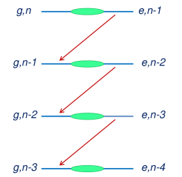
Figure 1: Energy diagram of the atom ($g$ for the ground state, $e$ for the excited one) dressed by laser photons (number $n$). States (blue lines) are grouped in twofold nearly degenerate multiplicities in which they are coupled by reversible absorption and stimulated emission processes (green shaded ellipses). Spontaneous emission processes are irreversible jumps downward the ladder of multiplicities (red arrows).

The fluorescence process appears as a succession of elementary processes sketched on the diagram of Fig.1. Absorption and stimulated emission of laser photons by the atom are described by the reversible evolution in a given multiplicity $\mathcal{E}_{n}$ while spontaneous emission processes correspond to irreversible jumps from a multiplicity $\mathcal{E}_{n}$ to the adjacent lower one $\mathcal{E}_{n-1}$. The random jumps interrupt the reversible evolution while projecting the atom from the excited to the ground state [25].

With the dependence of $\Omega$ versus $n$ neglected, the diagram of Fig.1 is stationary under changes of $n$, and it is tempting to fold up the multiplicities on a density matrix describing the atom-field system, thus reproducing the master equation commonly used to study resonance fluorescence [16, 17, 18, 19, 20]. The drawback of this method is that the reversible and irreversible processes are mixed up in the folding process, resulting in a dilution of their intrinsic difference.

A much better way to proceed is to go on with the full diagram of Fig.1 which keeps the trace of the number of fluorescence photons. The full process is called a radiative cascade because of its analogy to cascades happening in atomic or nuclear configurations with successive transitions [28]. It has been described by master equation techniques derived from general relaxation theory [26, 27], also using the sophisticated methods of photodetection theory [29, 30, 31]. Here we use a more intuitive approach which gives direct access to the distribution of delays between successively emitted photons, while producing the same results as master equation techniques.

The evolution is written for a wave function defined in a multiplicity $\mathcal{E}_{n}$ (the initial value of $n$ being irrelevant thanks to the stationarity of the diagram of Fig.1)

$$\left|\Psi_{n}\left(\tau\right)\right>=a_{n}\left(\tau\right)\left|g,n\right>+b_{n}\left(\tau\right)\left|e,n-1\right>~{},$$ (1)

$$a_{n}^{\prime}=-\imath\frac{\Omega}{2}b_{n}~{},\quad b_{n}^{\prime}=-\imath\frac{\Omega}{2}a_{n}-\left(\gamma-\imath\delta\right)b_{n}~{},$$

where the prime symbol denotes a derivation with respect to time $\tau$. With the initial state set just after the detection of a fluorescence photon, that is also just after a projection in the ground state ($a_{n}(0)=1$, $b_{n}(0)=0$), these equations are solved as

$$a_{n} =\left(\cosh\frac{\chi\tau}{2}+\frac{\gamma-\imath\delta}{\chi}\sinh\frac{\chi\tau}{2}\right)e^{-\left(\gamma-\imath\delta\right)\frac{\tau}{2}}~{},$$ (2)

$$b_{n} =-\frac{\imath\Omega}{\chi}\sinh\frac{\chi\tau}{2}e^{-\left(\gamma-\imath\delta\right)\frac{\tau}{2}}~{},$$

$$\chi =\sqrt{\left(\gamma-\imath\delta\right)^{2}-\Omega^{2}}~{}.$$

We also define the populations in the two states of the multiplicity $\mathcal{E}_{n}$

$$|a_{n}|^{2} =\left|\cosh\frac{\chi\tau}{2}+\frac{\gamma-\imath\delta}{\chi}\sinh\frac{\chi\tau}{2}\right|^{2}e^{-\gamma\tau}~{},$$ (3)

$$|b_{n}|^{2} =\left|\frac{\Omega}{\chi}\sinh\frac{\chi\tau}{2}\right|^{2}e^{-\gamma\tau}~{}.$$

At resonance, $\chi$ is real for $\Omega<\gamma$ and purely imaginary for $\Omega>\gamma$. The forms (2-3) have to be taken as the limits for $\chi\to 0$ at the border $\Omega=\gamma$ (for $\delta=0$).

We now define the delay function $K$ (called the waiting function $W$ in [32]) which is the probability of emission of the next fluorescence photon at time $\tau$ after an emission at time 0. It is the product of the Einstein coefficient $\Gamma=2\gamma$ by the population $|b_{n}|^{2}$ calculated in (3) for an atom in the ground state at $\tau=0$

$$K\left(\tau\right)=2\gamma|b_{n}|^{2}=-P^{\prime}\left(\tau\right)\,,\quad P\left(\tau\right)=|a_{n}|^{2}+|b_{n}|^{2}~{}.$$ (4)

The fact that $K$ is the opposite of time derivative of the total population $P$ in $\mathcal{E}_{n}$ is an immediate consequence of equations (1). It means that $K$ is the feeding rate of population in the adjacent lower multiplicity $\mathcal{E}_{n-1}$, starting a new reversible evolution in $\mathcal{E}_{n-1}$ which leads to the next fluorescence event. Equation (4) implies that the cumulative distribution function for the emission of the next fluorescence photon is $1-P(\tau)$, going from 0 to 1 when $\tau$ runs from 0 to $\infty$. Hence, the intensity $K(\tau)$ has a unity integral when integrated over $\tau$.

We stress at this point that the fluorescence process is intrinsically random. As we consider only signals built on the fluorescence intensity, the process can be understood as a series of random times of emission of successive photons. Each of the independent random delays are characterized by the delay function $K$ or, equivalently, by a non stationary Poisson point process [21, 22, 23]

$$\Lambda\left(\tau\right)=\ln\frac{1}{P\left(\tau\right)}~{},\quad\lambda\left(\tau\right)\equiv\Lambda^{\prime}\left(\tau\right)=\frac{K\left(\tau\right)}{P\left(\tau\right)}~{},$$ (5)

$$K\left(\tau\right)=\lambda\left(\tau\right)\exp\left(-\Lambda\left(\tau\right)\right)~{}.$$

The non stationary Poisson intensity $\lambda(\tau)$ is defined from $K(\tau)$ after a division by the total population $P(\tau)$ still in $\mathcal{E}_{n}$ at time $\tau$. It would be constant for a normal Poisson process, but this is not the case here as $\lambda(\tau)$ starts from a null value at $\tau=0$.

III Photon counting statistics

We now discuss the photon counting statistics which has been studied theoretically [14, 27, 33, 34, 35, 36] and experimentally [15, 37, 38, 39]. It reveals non trivial statistics of the number $N_{T}$ of fluorescence photons emitted in a given time interval $T$, which may possibly be sub-Poissonian, that is more regular than standard Poisson statistics.

Here, we derive the counting statistics from the delay function [26, 27, 32], using the relations discussed for more general point processes in [40]. We first study the random variable $t_{n}$ defined as the time of emission of the $n-$th photon after the emission of a $0-$th photon. With $t_{0}$ set to 0, $t_{n}$ is the sum of $n$ successive delays (as far as possible, we use $\tau$ for delays between successive emissions and $t$ for emission times)

$$t_{n}\equiv\tau_{1}+\tau_{2}+\ldots+\tau_{n}~{}.$$ (6)

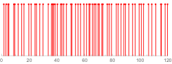
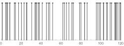
Figure 2: Random draw of a series of fluorescence times (red, upper plot) for $\Omega=\sqrt{2}\gamma,\delta=0$, compared to a standard Poisson process with the same mean delay (gray, lower plot). Time is measured by the dimensionless variable $\gamma t_{n}$.

An example of series of $t_{n}$ is shown on the upper plot of Fig.2 by successive red bars, with random delays drawn with the distribution $K$ calculated for $\Omega=\sqrt{2}\gamma$ and $\delta=0$. Each delay is obtained as $P^{(-1)}(u)$ where $P^{(-1)}$ is the inverse function of $P$ while $u$ is a random variable with a uniform distribution on $\left[0,1\right]$. The parameters are chosen so that the flow of photons shows a good regularity, with a large noise reduction compared to the standard Poisson noise. On Fig.2, the regularity is seen through a comparison with a Poissonian flow on the lower plot (calculated with the same mean delay). A clearer representation of the regularity property is shown by the histograms on Fig.3, corresponding to random draws of 10000 delays in the sub-Poissonian and Poissonian distributions. Other characterizations will be discussed below.

As the different delays are independent random variables with identical probability distribution $K$, the distribution $K_{n}$ of $t_{n}$ is given by a repeated convolution on $K$ ($\otimes$ representing a convolution product)

$$K_{1}\equiv K~{},\quad K_{2}\equiv K\otimes K_{1}~{},\quad K_{n}=K\otimes K_{n-1}~{}.$$ (7)

This leads to simple algebraic relations between the Laplace transforms of the functions

$$\widetilde{K}\left(s\right)=\int_{0}^{\infty}e^{-s\tau}K\left(\tau\right)\mathrm{d}\tau~{},$$ (8)

$$\widetilde{K}_{n}\left(s\right)=\left(\widetilde{K}\left(s\right)\right)^{n}~{}.$$

In particular, one easily gets the mean value and variance of $t_{n}$ from those of $\tau$

$$\overline{t}_{n}=n\overline{\tau}~{},\quad\Delta t_{n}^{2}=n\Delta\tau^{2}~{}.$$ (9)

Figure 3: Probability per channel for 10000 random delays drawn for $\Omega=\sqrt{2}\gamma,\delta=0$ (red), compared to a standard Poisson process with the same mean delay (gray). Delay is measured by the dimensionless variable $\gamma\tau$.

The Laplace transform $\widetilde{K}(s)$ can be written as a rational function since $K(\tau)$ is a sum of exponential functions

$$\widetilde{K}\left(s\right)=\frac{\gamma\Omega^{2}(s+\gamma)}{s(s+2\gamma)\left((s+\gamma)^{2}+\delta^{2}\right)+\Omega^{2}(s+\gamma)^{2}}~{},$$ (10)

with $\widetilde{K}(0)=1$ as a consequence of the normalization of $K(\tau)$. The mean $\overline{\tau}$ and variance $\Delta\tau^{2}$ of $\tau$ can be computed through derivations of $\ln\widetilde{K}(s)$

$$\overline{\tau} =-\left(\ln\widetilde{K}\right)^{\prime}_{s=0}=\frac{2\left(\gamma^{2}+\delta^{2}\right)+\Omega^{2}}{\gamma\Omega^{2}}~{},$$ (11)

$$\Delta\tau^{2} =\overline{\tau^{2}}-\overline{\tau}^{2}=\left(\ln\widetilde{K}\right)^{\prime\prime}_{s=0}$$

$$=\frac{4\left(\gamma^{2}+\delta^{2}\right)^{2}+2\left(3\delta^{2}-\gamma^{2}\right)\Omega^{2}+\Omega^{4}}{\gamma^{2}\Omega^{4}}~{}.$$

We study now the counting statistics of the number $N_{T}$ of fluorescence photons emitted during a given time interval $T$, assuming that $T$ is long enough so that the number $N_{T}$ is large. The statistical distribution of $N_{T}$ thus tends to be Gaussian as a consequence of the central limit theorem. It is then easy to infer the nearly Gaussian counting statistics of $N_{T}$ from that of $t_{n}$ with the following mean value and variance [27, 33, 32]

$$\overline{N}_{T}=\frac{T}{\overline{\tau}}\,,\quad\Delta N_{T}^{2}=\overline{N}_{T}\frac{\Delta\tau^{2}}{\overline{\tau}^{2}}=\overline{N}_{T}\left(1+Q\right)~{},$$ (12)

$$Q\equiv\frac{\Delta\tau^{2}}{\overline{\tau}^{2}}-1=\frac{2\left(\delta^{2}-3\gamma^{2}\right)\Omega^{2}}{\left(2\left(\gamma^{2}+\delta^{2}\right)+\Omega^{2}\right)^{2}}~{}.$$

The variance $\Delta N_{T}^{2}$ scales versus $T$ as the mean $\overline{N}_{T}$, and the ratio between these quantities is usually written in terms of the $Q-$factor introduced by Mandel [14]. This factor is interpreted here from its definition in (12).

Negative values of $Q$ correspond to sub-Poissonian statistics with photon number fluctuations smaller than in standard Poisson statistics, They are obtained when the detuning is not too large ($\delta^{2}<3\gamma^{2}$). In particular $Q_{0}$, $Q$ at resonance ($\delta=0$), is negative for any $\Omega$

$$Q_{0}=-\frac{3\Omega_{\mathrm{opt}}^{2}\Omega^{2}}{\left(\Omega_{\mathrm{opt}}^{2}+\Omega^{2}\right)^{2}}~{},\quad\Omega_{\mathrm{opt}}=\sqrt{2}\gamma~{}.$$ (13)

A value $Q_{\mathrm{opt}}=-\tfrac{3}{4}$ is obtained at $\Omega=\Omega_{\mathrm{opt}}$ which gives in principle an optimal reduction $1+Q_{\mathrm{opt}}=\tfrac{1}{4}$ with respect to standard Poisson noise. This corresponds to the regular flow shown on the upper plot of Fig.2 and on Fig.3. Experimentally obtained reductions are smaller than that as the detrimental effect of imperfect detection efficiency has to be accounted for [14, 27].

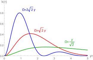
Figure 4: Dimensionless function $k=K/\gamma$ drawn versus dimensionless delay $\gamma\tau$ for $\Omega=\Omega_{\mathrm{opt}}=\sqrt{2}\gamma$ (red), $\Omega=\Omega_{\mathrm{opt}}/2$ (green) and $\Omega=2\Omega_{\mathrm{opt}}$ (blue) at resonance ($\delta=0$).

We note that the same value $Q_{0}$ is obtained in (13) for values of $\Omega$ forming a geometric progression around the optimum $\Omega_{\mathrm{opt}}$ (for example $1+Q_{0}=\frac{13}{25}$ for $\Omega=\Omega_{\mathrm{opt}}/2$ and $\Omega=2\Omega_{\mathrm{opt}}$). But the functions $K(\tau)$, drawn on Fig.4 with the optimal case, have different shapes in these two cases, which means that $Q$ is not a full characterization of the photon statistics. A more complete characterization will be given in the next section.

IV Photon correlation

We then discuss the photon correlation signal which has been studied theoretically [17, 18, 19, 20] and experimentally [12, 13]. This correlation reveals the antibunching effect which has been used as a characterization tool for a large variety of systems of physical interest [41, 42, 43, 44, 45, 46, 47, 48, 49, 50, 51, 52, 53, 54, 55, 56, 57, 58].

The intensity correlation signal $C_{I}(t)$ is associated to the detection of a fluorescence photon at time $t_{0}$ and another one at time $t_{0}+t$. It does not depend on $t_{0}$ because of the stationarity of the mean intensity, so that the discussion is focused on the role of $t$. With $t_{0}$ set to 0, the time $t$ can be any of the times $t_{n}$ with $n=1,2,\ldots$, not necessarily the next one as in the definition of $K$. We then define the function $J(t)$ by using the results of the previous section

$$J\left(t\right)=K_{1}\left(t\right)+K_{2}\left(t\right)+\ldots+K_{n}\left(t\right)+\ldots~{}.$$ (14)

This relation takes a simple algebraic form when written in terms of Laplace transforms

$$\widetilde{J}\left(s\right)=\widetilde{K}+\widetilde{K}^{2}+\ldots+\widetilde{K}^{n}+\ldots=\frac{\widetilde{K}\left(s\right)}{1-\widetilde{K}\left(s\right)}~{}.$$ (15)

As $\widetilde{K}$ is a rational function of $s$, it is also true for $\widetilde{J}$

$$\widetilde{J}=\frac{\gamma}{s}\;\frac{\Omega^{2}\left(s+\gamma\right)}{(s+2\gamma)\left((s+\gamma)^{2}+\delta^{2}\right)+\Omega^{2}(s+\gamma)}~{}.$$ (16)

The function $\widetilde{J}(s)$ can itself be decomposed as a sum of elementary rational functions

$$\widetilde{J}\left(s\right)=\frac{\overline{I}}{s}+\Delta\widetilde{J}\left(s\right)~{},\quad\Delta\widetilde{J}\left(s\right)=\sum_{m=1}^{3}\frac{\rho_{m}}{s+r_{m}}~{},$$ (17)

where $\overline{I}$ is the mean intensity calculated as the residue associated with the pole of $\widetilde{J}$ at $s=0$, that is also the inverse of the mean delay given in (12)

$$\overline{I}=\lim_{s\to 0}\left(s\widetilde{J}\left(s\right)\right)=\frac{\gamma\Omega^{2}}{2\left(\gamma^{2}+\delta^{2}\right)+\Omega^{2}}=\frac{1}{\overline{\tau}}~{},$$ (18)

while the $r_{m}$’s are the opposite of non null roots of the denominator of $\widetilde{J}$ and the $\rho_{m}$’s the associated residues.

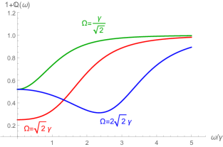
Figure 5: Function $1+Q(\omega)$ representing the reduction of standard Poisson noise versus dimensionless frequency $\omega/\gamma$ with the same parameters and color codes as on Fig.4.

We do not write explicitly the roots and residues which are readily obtained by solving a cubic equation with formal or numerical software. The function $J(t)$ is deduced as a sum (Heaviside functions $\theta(t)$ inserted to emphasize that $J(t)$ and $\Delta J(t)$ are defined for $t\geq 0$)

$$J\left(t\right)=\overline{I}\,\theta\left(t\right)+\Delta J\left(t\right)~{},$$ (19)

$$\Delta J\left(t\right)=\theta\left(t\right)\sum_{m=1}^{3}\rho_{m}e^{-r_{m}t}~{}.$$

The photon correlation function $C_{I}(t)$ is then obtained in terms of already introduced functions (details in the Appendix B of [40])

$$C_{I}\left(t\right)=\overline{I}\left(\overline{I}\,\delta\left(t\right)+\Delta J\left(t\right)+\Delta J\left(-t\right)\right)~{}.$$ (20)

The first term in the parenthesis corresponds to the detection of the same photon at $t_{0}=0$ and $t$ and it involves a Dirac function $\delta(t)$ describing this simultaneity. The second and third terms represent the detection of photons at $t\neq t_{0}$ with $t>t_{0}$ and $t<t_{0}$ respectively.

Another interesting characterization is the photon noise spectrum $S_{I}(\omega)$ defined as the Fourier transform of $C_{I}(t)$ which can be measured by sending the intensity signal to a spectrum analyzer. We obtain for this signal (see the Appendix B of [40])

$$S_{I}\left(\omega\right)=\overline{I}\left(1+Q\left(\omega\right)\right)~{},$$ (21)

$$Q\left(\omega\right)=\Delta\widetilde{J}\left(\imath\omega\right)+\Delta\widetilde{J}\left(-\imath\omega\right)~{}.$$

The function $\Delta\widetilde{J}(s)$, written from $\widetilde{J}$ and $\overline{I}$

$$\Delta\widetilde{J}\left(s\right)=\frac{\overline{I}\left(\gamma^{2}+\delta^{2}-(s+2\gamma)^{2}\right)}{(s+2\gamma)\left((s+\gamma)^{2}+\delta^{2}\right)+\Omega^{2}(s+\gamma)}~{},$$ (22)

is regular at $s=0$ where its value is directly related to the Mandel $Q-$factor, as $Q(0)=2\Delta\widetilde{J}(0)\equiv Q$.

Hence, $Q(\omega)$ is a generalization of the $Q-$factor, showing sub-Poissonian noise at non zero frequencies. Examples of the function $1+Q(\omega)$ are drawn on Fig.(5) for the same parameters and color codes as on Fig.(4). The red curve corresponds to the optimal reduction with $1+Q=\tfrac{1}{4}$ at null frequency then increasing to reach the standard value 1 at large frequencies. The two other curves correspond to the same value of $Q$ at null frequency, but they show different behaviours as functions of $\omega$, which means that $Q(\omega)$ contains more information on photon statistics than $Q(0)$.

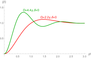
Figure 6: Dimensionless function $j=J/\overline{I}$ drawn versus dimensionless time $\gamma t$ for $\Omega=2.2\gamma$ (red) and $\Omega=4.4\gamma$ (green) at resonance ($\delta=0$). These functions match those drawn on Fig.4 of ref.[13] calculated for the same parameters.

Note that sub-Poissonian statistics opened the way [59] to the study of squeezing, with a large number of applications, for which we quote a few reviews [60, 61, 62, 63, 64, 65, 66, 67, 68, 69].

V Comparison with literature

We now emphasize that the expressions given in this review match those written in many papers in the existing literature, with some of them shown to agree with the results of dedicated experiments.

In the case of resonant excitation, $j_{0}$ ($j\equiv J/{\overline{I}}$ calculated for $\delta=0$) has the following form

$$j_{0}\left(t\right)=1-e^{-\frac{3\gamma t}{2}}\left(\cosh\left(\digamma t\right)+\frac{3\gamma}{2\digamma}\sinh\left(\digamma t\right)\right)~{},$$ (23)

$$\overline{I}_{0}=\frac{\gamma\Omega^{2}}{2\gamma^{2}+\Omega^{2}}~{},\quad\digamma=\sqrt{\frac{\gamma^{2}}{4}-\Omega^{2}}~{},$$

which matches expressions written for example in [17, 12, 13, 14]. Figure (6) shows this function drawn versus the dimensionless time $\gamma t$ for two values of $\Omega$. They match those drawn on Fig.4 of ref.[13] calculated from equivalent formula and for the same parameters and also shown there to agree with the results of experiments on the resonance fluorescence of laser-excited sodium atoms in an atomic beam. Functions $j$ defined analogously for non resonant excitation are shown on Fig.(7) and they match those drawn on Fig.5 of ref.[13].

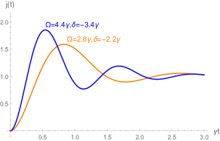
Figure 7: Dimensionless function $j=J/\overline{I}$ drawn versus $\gamma t$ for the parameters $\Omega=2.8\gamma,\delta=-2.2\gamma$ (orange) and $\Omega=4.4\gamma,\delta=-3.4\gamma$ (blue). These functions match those on Fig.5 of ref.[13] calculated for the same parameters.

Differences have been noticed between the predictions in [21, 22, 23] and those of the present method, with these differences large in the weak-excitation limit where the Rabi frequency $\Omega$ remains small compared to $\gamma\,,\delta$ (see Fig.2 in ref.[23]). This is why we discuss also this limit, in which a good approximation is obtained by a perturbative expansion of the correlation function in terms of photon scattering amplitudes [70]

$$j_{\mathrm{pert}}\equiv J_{\mathrm{pert}}/{\overline{I}_{\mathrm{pert}}}=\left|1-e^{-\left(\gamma-\imath\delta\right)t}\right|^{2}~{},$$ (24)

$$\overline{I}_{\mathrm{pert}}=\frac{\gamma\Omega^{2}}{2\left(\gamma^{2}+\delta^{2}\right)}~{}.$$

The amplitudes interfering in eq.(24) are two-photon scattering amplitudes which are sufficient to describe the fluorescence process in this limit. They correspond to two independent elastic Rayleigh scatterings (each linear in the field amplitude) on one hand, and one inelastic two-photon scattering (quadratic in the field amplitude) on the other hand. Again, this expression matches the results written above in the weak-excitation limit.

In this limit, the fluorescence flux is weak and experiments are more delicate than those corresponding to a higher flux. There are however configurations directly related to this discussion for which experiments have been performed and have confirmed the scattering formalism. When filters are used to select the inelastic scattering spectral lines, the interference leading to antibunching is destroyed but a bunching signal remains which is characteristic of the inelastic two-photon fluorescence process [25, 26]. This signal has been observed experimentally and found to agree with the theory [71] (see also [72, 73, 74] for recent discussions of correlations between frequency filtered photons). Another configuration corresponds to multiatom resonance fluorescence where photon antibunching has been observed in the field emitted coherently by many atoms under conditions of phase-matching [75] and found to agree with the theory [76].

VI Conclusion

In this paper, we have reviewed the understanding of the radiative cascade of resonance fluorescence photons emitted by a laser-excited two-level atom. We have considered the delay function as the primary characterization of this random point process, and derived other statistical characterizations from it.

This method is perfectly adapted to the discussion of the quantum jumps observed when fluorescence is interrupted by shelving the atom on a long-lifetime trap level [77]. The experimental observation of these quantum jumps [78, 79, 80, 81, 82] was accompanied by a number of theoretical papers discussing this spectacular effect [83, 84, 85, 86, 87, 88]. The description in terms of momentary interruption of the radiative cascade of the dressed atom gave an extremely efficient and intuitive comprehension of intermittent fluorescence [89, 90].

Here, we considered only signals built on the fluorescence intensity, so that the process can be fully understood as a series of random times of emission of successive photons. The series can be drawn from independent random delays characterized by the function $K$ or, equivalently, by $P$, $\Lambda$ or $\lambda$. The intrinsic randomness of the process is also emphasized in the Monte-Carlo wave-function approach to dissipative spontaneous emission which allows one to study other observables [91, 92, 93, 94, 95, 96].

Acknowledgements: This paper is dedicated to the memory of Jean Ginibre who initiated with Yves Pomeau and Martine Le Berre stimulating discussions about the intrinsic randomness of resonance fluorescence emitted by a single atom. I also want to thank Claude Cohen-Tannoudji and Jean Dalibard for many discussions spread over years of fruitful collaboration.

References

- Planck [1900] M. Planck. Theory of the energy distribution law in the normal spectrum (in german). Deutsch. Phys. Ges., 2:237–245, 1900.
- Einstein [1905] A. Einstein. Generation and conversion of light with regard to a heuristic point of view (in german). Annalen der Physik, 17:132–148, 1905.
- Einstein [1909] A. Einstein. On the present status of the radiation problem (in german). Phys. Zeitschrift, 10:185–193, 1909.
- Einstein [1917] A. Einstein. Quantum theory of radiation (in german). Phys. Zeitschrift, 18:121–128, 1917.
- Dirac [1927] P. A. M. Dirac. The quantum theory of the emission and absorption of radiation. Proc. of the Royal Society A, 114:243–265, 1927.
- Weisskopf and Wigner [1930] V. Weisskopf and E. Wigner. Calculation of the natural width of line based on the Dirac’s theory of light (in german). Zeitschrift fur Physik, 63:54–73, 1930.
- Fermi [1932] E. Fermi. Quantum theory of radiation. Rev. Modern Phys., 4:87–132, 1932.
- Schuda et. al. [1974] F. Schuda, C. R. Stroud, and M. Hercher. Observation of resonant Stark effect at optical frequencies. Journal of Physics B, 7:L198–L202, 1974.
- Wu et. al. [1975] F. Y. Wu, R. E. Grove, and S. Ezekiel. Investigation of spectrum of resonance fluorescence induced by a monochromatic field. Phys. Rev. Letters, 35:1426–1429, 1975.
- Grove et. al. [1977] R. E. Grove, F. Y. Wu, and S. Ezekiel. Measurement of spectrum of resonance fluorescence from a 2-level atom in an intense monochromatic-field. Phys. Rev. A, 15:227–233, 1977.
- Ortiz-Gutiérrez et. al. [2019] L. Ortiz-Gutiérrez, R. Celistrino. Teixeira, A. Eloy, D. Ferreira da Silva, R. Kaiser, R. Bachelard, and M. Fouché. Mollow triplet in cold atoms. New Journal of Physics, 21:093019, 2019.
- Kimble et. al. [1977] H. J. Kimble, M. Dagenais, and L. Mandel. Photon anti-bunching in resonance fluorescence. Phys. Rev. Letters, 39:691–695, 1977.
- Dagenais and Mandel [1978] M. Dagenais and L. Mandel. Investigation of 2-time correlations in photon emissions from a single atom. Phys. Rev. A, 18:2217–2228, 1978.
- Mandel [1979] L. Mandel. Sub-Poissonian photon statistics in resonance fluorescence. Optics Letters, 4:205–207, 1979.
- Short and Mandel [1983] R. Short and L. Mandel. Observation of sub-Poissonian photon statistics. Phys. Rev. Letters, 51:384–387, 1983.
- Mollow [1969] B. R. Mollow. Power spectrum of light scattered by two-level systems. Phys. Rev., 188:1969–1975, 1969.
- Carmichael and Walls [1976a] H. J. Carmichael and D. F. Walls. Proposal for the measurement of the resonant Stark effect by photon correlation techniques. Journal of Physics B, 9:L43–L46, 1976a.
- Carmichael and Walls [1976b] H. J. Carmichael and D. F. Walls. Quantum-mechanical master equation treatment of dynamical Stark effect. Journal of Physics B, 9:1199–1219, 1976b.
- Kimble and Mandel [1976] H. J. Kimble and L. Mandel. Theory of resonance fluorescence. Phys. Rev. A, 13:2123–2144, 1976.
- Cohen-Tannoudji [1977] C. Cohen-Tannoudji. Atoms in strong resonant fields. In R. Balian, S. Haroche, and S. Liberman, editors, Frontiers in laser spectroscopy, Les Houches Summer School (1975), pages 1–104. North Holland, 1977.
- Pomeau et. al. [2016] Y. Pomeau, M. Le Berre, and J. Ginibre. Ultimate statistical physics: fluorescence of a single atom. J. Statistical Mechanics-Theory and Experiment, 2016:104002, 2016.
- Pomeau and Le Berre [2021] Y. Pomeau and M. Le Berre. Randomness and irreversiblity in quantum mechanics: A worked example for a statistical theory. Entropy, 23:1643, 2021.
- Pomeau and Le Berre [2022] Y. Pomeau and M. Le Berre. Quantum mechanics: how to use Everett theory practically. EPJ Web Conf., 263:01010, 2022.
- Cohen-Tannoudji and Reynaud [1977] C. Cohen-Tannoudji and S. Reynaud. Dressed-atom description of resonance fluorescence and absorption-spectra of a multilevel atom in an intense laser-beam. Journal of Physics B, 10:345–363, 1977.
- Cohen-Tannoudji and Reynaud [1979] C. Cohen-Tannoudji and S. Reynaud. Atoms in strong light-fields: photon antibunching in single atom fluorescence. Philosophical Transactions of the Royal Society A, 293:223–237, 1979.
- Reynaud [1981] S. Reynaud. Resonant interaction of an atom with a monochromatic intense laser wave (in french). https://tel.archives-ouvertes.fr/tel-00011837, 1981. Thèse d’Etat de l’Université Pierre et Marie Curie.
- Reynaud [1983] S. Reynaud. Resonance fluorescence: the dressed atom approach (in french). Annales de Physique, 8:315–370, 1983.
- Popp et. al. [1970] M. Popp, G. Schafer, and E. Bodenstedt. Investigation of photon-photon angular correlations in atomic mercury. Zeitschrift fur Physik, 240:71, 1970.
- Glauber [1963] R. J. Glauber. Quantum theory of optical coherence. Phys. Rev., 130:2529–&, 1963.
- Kelley and Kleiner [1964] P. L. Kelley and W. H. Kleiner. Theory of electromagnetic field measurement + photoelectron counting. Phys. Rev., 136:A316, 1964.
- Davidson and Mandel [1968] F. Davidson and L. Mandel. Photoelectric correlation measurements with time-to-amplitude converters. J. Appl. Phys., 39:62–&, 1968.
- Reynaud et. al. [1988] S. Reynaud, J. Dalibard, and C. Cohen-Tannoudji. Photon statistics and quantum jumps: the picture of the dressed atom radiative cascade. IEEE J. Quantum Electronics, 24:1395–1402, 1988.
- Kim et. al. [1987] M. S. Kim, P. L. Knight, and K. Wodkiewicz. Correlations between successively emitted photons in resonance fluorescence. Optics Communications, 62:385–388, 1987.
- Carmichael et. al. [1989] H. J. Carmichael, S. Singh, R. Vyas, and P. R. Rice. Photoelectron waiting times and atomic state reduction in resonance fluorescence. Phys. Rev. A, 39:1200–1218, 1989.
- Kim and Knight [1989] M. S. Kim and P. L. Knight. Photon correlations and successive emission. Phys. Rev. A, 40:215–227, 1989.
- Davidovich [1996] L. Davidovich. Sub-Poissonian processes in quantum optics. Rev. Modern Phys., 68:127–173, 1996.
- Schubert et. al. [1992] M. Schubert, I. Siemers, R. Blatt, W. Neuhauser, and P. E. Toschek. Photon antibunching and non-Poissonian fluorescence of a single 3-level ion. Phys. Rev. Letters, 68:3016–3019, 1992.
- Fleury et. al. [2000] L. Fleury, J. M. Segura, G. Zumofen, B. Hecht, and U. P. Wild. Nonclassical photon statistics in single-molecule fluorescence at room temperature. Phys. Rev. Letters, 84:1148–1151, 2000.
- Treussart et. al. [2004] F. Treussart, R. Alleaume, J.-M. Courty, and J.-F. Roch. Emission properties of a single photon source. Physica Scripta, T112:95–98, 2004.
- Reynaud [1990] S. Reynaud. An introduction to the reduction of quantum noise (in french). Annales de Physique, 15:63–162, 1990.
- Diedrich and Walther [1987] F. Diedrich and H. Walther. Nonclassical radiation of a single stored ion. Phys. Rev. Letters, 58(3):203–206, 1987.
- Basche et. al. [1992] T. Basche, W. E. Moerner, M. Orrit, and H. Talon. Photon antibunching in the fluorescence of a single dye molecule trapped in a solid. Phys. Rev. Letters, 69:1516–1519, 1992.
- Schadwinkel et. al. [2000] H. Schadwinkel, V. Gomer, U. Reiter, B. Ueberholz, and D. Meschede. Quantum fluctuations of a single trapped atom: Transient Rabi oscillations and magnetic bistability. IEEE J. Quantum Electronics, 36:1358–1363, 2000.
- Michler et. al. [2000] P. Michler, A. Imamoglu, M. D. Mason, P. J. Carson, G. F. Strouse, and S. K. Buratto. Quantum correlation among photons from a single quantum dot at room temperature. Nature, 406:968–970, 2000.
- Brouri et. al. [2000] R. Brouri, A. Beveratos, J.-P. Poizat, and P. Grangier. Photon antibunching in the fluorescence of individual color centers in diamond. Optics Letters, 25:1294–1296, 2000.
- Leibfried et. al. [2003] D. Leibfried, R. Blatt, C. Monroe, and D. Wineland. Quantum dynamics of single trapped ions. Rev. Modern Phys., 75:281–324, 2003.
- Hennrich et. al. [2005] M. Hennrich, A. Kuhn, and G. Rempe. Transition from antibunching to bunching in cavity qed. Phys. Rev. Letters, 94:053604, 2005.
- Lounis and Orrit [2005] B. Lounis and M. Orrit. Single-photon sources. Reports on Progress in Physics, 68(5):1129–1179, 2005.
- Darquie et. al. [2005] B. Darquie, M. P. A. Jones, J. Dingjan, J. Beugnon, S. Bergamini, Y. Sortais, G. Messin, A. Browaeys, and P. Grangier. Controlled single-photon emission from a single trapped two-level atom. Science, 309:454–456, 2005.
- Beugnon et. al. [2006] J. Beugnon, M. P. A Jones, J. Dingjan, B. Darquie, G. Messin, A. Browaeys, and P. Grangier. Quantum interference between two single photons emitted by independently trapped atoms. Nature, 440:779–782, 2006.
- Zinoni et. al. [2006] C. Zinoni, B. Alloing, C. Monat, V. Zwiller, L. H. Li, A. Fiore, L. Lunghi, A. Gerardino, H. de Riedmatten, H. Zbinden, and N. Gisin. Time-resolved and antibunching experiments on single quantum dots at 1300 nm. Appl. Phys. Letters, 88:131102, 2006.
- Press et. al. [2007] D. Press, S. Gatzinger, S. Reitzenstein, C. Hofmann, A. Loffler, M. Kamp, A. Forchel, and Y. Yamamoto. Photon antibunching from a single quantum-dot-microcavity system in the strong coupling regime. Phys. Rev. Letters, 98:117402, 2007.
- Hagele et. al. [2008] A. Hagele, C. Galland, M. Winger, and A. Imamoglu. Photon antibunching in the photoluminescence spectra of a single carbon nanotube. Phys. Rev. Letters, 100:217401, 2008.
- Gerber et. al. [2009] S. Gerber, D. Rotter, L. Slodicka, J. Eschner, H. J. Carmichael, and R. Blatt. Intensity-field correlation of single-atom resonance fluorescence. Phys. Rev. Letters, 102:183601, 2009.
- Heine et. al. [2009] D. Heine, M. Wilzbach, T. Raub, B. Hessmo, and J. Schmiedmayer. Integrated atom detector: Single atoms and photon statistics. Phys. Rev. A, 79:021804, 2009.
- Lupton and Vogelsang [2021] J. M. Lupton and J. Vogelsang. Photon correlations probe the quantized nature of light emission from optoelectronic materials. Appl. Phys. Rev., 8:041302, 2021.
- Avriller et. al. [2021] R. Avriller, Q. Schaeverbeke, T. Frederiksen, and F. Pistolesi. Photon-emission statistics induced by electron tunneling in plasmonic nanojunctions. Phys. Rev. B, 104:L241403, 2021.
- Darsheshdar et. al. [2021] E. Darsheshdar, M. Hugbart, R. Bachelard, and C. J. Villas-Boas. Photon-photon correlations from a pair of strongly coupled two-level emitters. Phys. Rev. A, 103:053702, 2021.
- Mandel [1982] L. Mandel. Squeezed states and sub-Poissonian photon statistics. Phys. Rev. Letters, 49:136–138, 1982.
- Walls [1983] D. F. Walls. Squeezed states of light. Nature, 306(5939):141–146, 1983.
- Loudon and Knight [1987] R. Loudon and P. L. Knight. Squeezed light - introduction. Journal of Modern Optics, 34:709–759, 1987.
- Kimble and Walls [1987] H. J. Kimble and D. F. Walls. Squeezed states of the electromagnetic-field - introduction. J. Opt. Soc. Am. B, 4:1450, 1987.
- Walls [1990] D. F. Walls. Nonclassical optical phenomena. Science Progress, 74:291–310, 1990.
- Reynaud et. al. [1992] S. Reynaud, A. Heidmann, E. Giacobino, and C. Fabre. Quantum fluctuations in optical systems. Progress in Optics, 30:1–85, 1992.
- Dodonov [2002] V. V. Dodonov. Nonclassical states in quantum optics: a squeezed review of the first 75 years. Quantum and Semiclassical Optics, 4:R1–R33, 2002.
- Schnabel et. al. [2010] R. Schnabel, N. Mavalvala, D. E. McClelland, and P. K. Lam. Quantum metrology for gravitational wave astronomy. Nature Communications, 1:121, 2010.
- Andersen et. al. [2016] U. L Andersen, T. Gehring, C. Marquardt, and G. Leuchs. 30 years of squeezed light generation. Physica Scripta, 91:053001, 2016.
- Schnabel [2017] R. Schnabel. Squeezed states of light and their applications in laser interferometers. Physics Reports, 684:1–51, 2017.
- Fabre and Treps [2020] C. Fabre and N. Treps. Modes and states in quantum optics. Rev. Modern Phys., 92:035005, 2020.
- Dalibard and Reynaud [1983] J. Dalibard and S. Reynaud. Correlation signals in resonance fluorescence - interpretation via photon scattering-amplitudes. Journal de Physique, 44:1337–1343, 1983.
- Aspect et. al. [1980] A. Aspect, G. Roger, S. Reynaud, J. Dalibard, and C. Cohen-Tannoudji. Time correlations between the 2 sidebands of the resonance fluorescence triplet. Phys. Rev. Letters, 45:617–620, 1980.
- López Carreño et. al. [2018] J. C. López Carreño, E. del Valle, and F.. P. Laussy. Frequency-resolved Monte Carlo. Scientific Reports, 8:6975, 2018.
- Phillips et. al. [2020] C. L. Phillips, A. J. Brash, D. P. S. McCutcheon, J. Iles-Smith, E. Clarke, B. Royall, M. S. Skolnick, A. M. Fox, and A. Nazir. Photon statistics of filtered resonance fluorescence. Phys. Rev. Letters, 125:043603, 2020.
- Hanschke et. al. [2020] L. Hanschke, L. Schweickert, J. C. López Carreño, E. Schöll, K. D. Zeuner, T. Lettner, E. Zubizarreta Casalengua, M. Reindl, S. F. Covre da. Silva, R. Trotta, J. J. Finley, A. Rastelli, E. del Valle, F. P. Laussy, V. Zwiller, K. Müller, and K. D. Jöns. Origin of antibunching in resonance fluorescence. Phys. Rev. Letters, 125:170402, 2020.
- Grangier et. al. [1986] P. Grangier, G. Roger, A. Aspect, A. Heidmann, and S. Reynaud. Observation of photon antibunching in phase-matched multiatom resonance fluorescence. Phys. Rev. Letters, 57:687–690, 1986.
- Heidmann and Reynaud [1985] A. Heidmann and S. Reynaud. Squeezing in the many atom resonance fluorescence emitted in the forward direction - application to photon noise-reduction. Journal de Physique, 46:1937–1948, 1985.
- Dehmelt [1982] H. G. Dehmelt. Mono-ion oscillator as potential ultimate laser frequency standard. IEEE Transactions on Instrumentation and Measurement, 31:83–87, 1982.
- Nagourney et. al. [1986] W. Nagourney, J. Sandberg, and H. Dehmelt. Shelved optical electron amplifier - observation of quantum jumps. Phys. Rev. Letters, 56:2797–2799, 1986.
- Sauter et. al. [1986] T. Sauter, W. Neuhauser, R. Blatt, and P. E. Toschek. Observation of quantum jumps. Phys. Rev. Letters, 57:1696–1698, 1986.
- Bergquist et. al. [1986] J. C. Bergquist, R. G. Hulet, W. M. Itano, and D. J. Wineland. Observation of quantum jumps in a single atom. Phys. Rev. Letters, 57:1699–1702, 1986.
- Finn et. al. [1986] M. A. Finn, G. W. Greenlees, and D. A. Lewis. Experimental evidence for quantum jumps in three-level systems. Optics Communications, 60:149–153, 1986.
- Itano et. al. [2015] W. M. Itano, J. C. Bergquist, and D. J. Wineland. Early observations of macroscopic quantum jumps in single atoms. Int. J. of Mass Spectrometry, 377:403–409, 2015.
- Cook and Kimble [1985] R. J. Cook and H. J. Kimble. Possibility of direct observation of quantum jumps. Phys. Rev. Letters, 54:1023–1026, 1985.
- Javanainen [1986] J. Javanainen. Possibility of quantum jumps in a 3-level system. Phys. Rev. A, 33:2121–2123, 1986.
- Pegg et. al. [1986] D. T. Pegg, R. Loudon, and P. L. Knight. Correlations in light emitted by 3-level atoms. Phys. Rev. A, 33:4085–4091, 1986.
- Schenzle and Brewer [1986] A. Schenzle and R. G. Brewer. Macroscopic quantum jumps in a single atom. Phys. Rev. A, 34:3127–3142, 1986.
- Kimble et. al. [1986] H. J. Kimble, R. J. Cook, and A. L. Wells. Intermittent atomic fluorescence. Phys. Rev. A, 34:3190–3195, 1986.
- Zoller et. al. [1987] P. Zoller, M. Marte, and D. F. Walls. Quantum jumps in atomic systems. Phys. Rev. A, 35:198–207, 1987.
- Cohen-Tannoudji and Dalibard [1986] C. Cohen-Tannoudji and J. Dalibard. Single-atom laser spectroscopy - looking for dark periods in fluorescence light. Europhysics Letters, 1:441–448, 1986.
- Dalibard et. al. [1987] J. Dalibard, S. Reynaud, and C. Cohen-Tannoudji. The radiative cascade of the dressed atom (in french). In Interaction of Radiation with Matter, pages 29–48. Quaderni della Schola Normale Superiore, 1987.
- Dalibard et. al. [1992] J. Dalibard, Y. Castin, and K. Mølmer. Wave-function approach to dissipative processes in quantum optics. Phys. Rev. Letters, 68:580–583, 1992.
- Dum et. al. [1992] R. Dum, P. Zoller, and H. Ritsch. Monte Carlo simulation of the atomic master equation for spontaneous emission. Phys. Rev. A, 45:4879–4887, 1992.
- Mølmer et. al. [1993] K. Mølmer, Y. Castin, and J. Dalibard. Monte Carlo wave-function method in quantum optics. J. Opt. Soc. Am. B, 10:524–538, 1993.
- Plenio and Knight [1998] M. B. Plenio and P. L. Knight. The quantum-jump approach to dissipative dynamics in quantum optics. Rev. Modern Phys., 70:101–144, 1998.
- Daley [2014] A. J. Daley. Quantum trajectories and open many-body quantum systems. Advances in Physics, 63:77–149, 2014.
- Xu et. al. [2015] Q. Xu, E. Greplova, B. Julsgaard, and K. Mølmer. Correlation functions and conditioned quantum dynamics in photodetection theory. Physica Scripta, 90:128004, 2015.