Area law for steady states of detailed-balance local Lindbladians

Abstract

We study steady-states of quantum Markovian processes whose evolution is described by local Lindbladians. We assume that the Lindbladian is gapped and satisfies quantum detailed balance with respect to a unique full-rank steady state $\sigma$. We show that under mild assumptions on the Lindbladian terms, which can be checked efficiently, the Lindbladian can be mapped to a local Hamiltonian on a doubled Hilbert space that has the same spectrum, and a ground state that is the vectorization of $\sigma^{1/2}$. Consequently, we can use Hamiltonian complexity tools to study the steady states of such open systems. In particular, we show an area-law in the mutual information for the steady state of such 1D systems, together with a tensor-network representation that can be found efficiently.

1 Introduction

Understanding the structure and physical properties of open many-body quantum systems is a major problem in condensed matter physics. Over the years, these systems have been studied using a plethora of methods from statistical physics, many-body quantum theory and functional analysis. More recently, with the advent of quantum computation and quantum information, these systems have also been studied using techniques coming from quantum information. Coming from these research paradigms, one would typically want to understand the computational complexity of these systems, the type of entanglement and correlations that they can create, and whether or not they can be represented efficiently on a classical computer.

This line of research has been well-established in the context of closed systems. In particular, there are many results characterizing the complexity of ground states of local Hamiltonians defined on a lattice. For example, it has been shown that for several families of Hamiltonians it is QMA-hard to approximate the ground state energy [1, 2], implying that the ground state of such systems does not posses an efficient classical description unless QMA=NP. On the other hand, it is generally believed that gapped local Hamiltonians on a $D$-dimensional lattice satisfy an area-law of entanglement entropy [3] and can be well approximated by efficient tensor network states. This has been rigorously proven in 1D [4], with some partial results in higher dimension [5, 6, 7, 8, 9, 10, 11].

A natural question to ask is whether, and to what extent, tools and techniques that are used to analyze the complexity of ground states of closed systems can be used to study the complexity of steady states of open systems. Specifically, in this paper we consider open systems that are described by Markovian dynamics that is generated by a local Lindbladian superoperator $\mathcal{L}=\sum_{i}\mathcal{L}_{i}$ (see section 2 for a formal definition). The steady state of the system is then given by a density operator $\sigma$ for which

$$\mathcal{L}(\sigma)=\sum_{i}\mathcal{L}_{i}(\sigma)=0.$$

This is a homogeneous linear equation, which has a striking similarity to the corresponding problem in closed system

$$(H-\epsilon_{0}\mathbbm{1}){|{\Omega}\rangle}=\left(\sum_{i}h_{i}-\epsilon_{0}\mathbbm{1}\right){|{\Omega}\rangle}=0,$$

where $H=\sum_{i}h_{i}$ is a local Hamiltonian with ground state ${|{\Omega}\rangle}$ and ground energy $\epsilon_{0}$. Moreover, as described in section 2, the spectrum of $\mathcal{L}$ is in the $\textrm{Re}\leq 0$ part of the complex plane, and we can define the spectral gap of the Linbladian to be the largest non-zero real part of the spectrum. It is therefore tempting to try and use local Hamiltonian techniques to characterize $\sigma$. However, a quick inspection reveals the main obstacle for such a simple plan to work: Whereas the Hamiltonian is a self-adjoint (hermitian) operator, which therefore has a real spectrum with a set of orthonormal eigenstates, the same is not true for the Lindbladian; it is generally not a self-adjoint operator, and consequently its spectrum might be complex with non-orthogonal eigenoperators. To make $\mathcal{L}$ self-adjoint, one might consider $\mathcal{L}^{*}\mathcal{L}$, but this come at the price of losing locality. Alternatively, we might consider $\frac{1}{2}(\mathcal{L}+\mathcal{L}^{*})$, but it is not clear how the eigenstates of this operator are related to the eignstates of $\mathcal{L}$.

A more sophisticated way of obtaining self-adjointness is by assuming that the Linbladian satisfies quantum detailed-balance [12, 13]. For such Linbladians there is a way of defining an inner product with respect to which $\mathcal{L}$ is self-adjoint [13, 14, 15, 16] (see subsection 2.3). This inner product, however, can be highly non-local (with respect to the underlying tensor-product structure) and might deform the natural geometry of the Hilbert space. It is therefore not clear how to use it to bound correlations and other measures of locality in the steady state.

Nevertheless, in this paper we show that the quantum detailed-balance condition provides a surprisingly simple map that takes a local Lindbladian to a self-adjoint local super-operartor (i.e, a super Hamiltonian), which is then mapped to a local Hamiltonian using vectorization. All this is done while maintaining a direct relation between the steady state of the former and the ground state of the latter. Consequently, many of the bounds and properties that were proved for ground states, easily transform to the steady states of detailed-balance Lindbladians. In particular, we show that under mild conditions, which can be efficiently checked, steady states of gapped 1D Lindbladian with detailed balance satisfy an area-law for the mutual information. Moreover, just as in the 1D area-law case for local Hamiltonians, these steady states are well-approximated by an efficient tensor network.

We conclude this section by noting that our mapping is not new; it has already been used before, e.g., in Refs. [17, 15, 18, 19, 20]. Our main contribution is showing that this mapping results in a local Hamiltonian, rather than a general Hermitian operator, which enables us to take advantage of the local Hamiltonian machinery (see subsection 3.1).

1.1 Comparison with previous works

Several works studied the entanglement structure of steady states of open systems, see for example Refs.  [18, 21, 22, 23]. Here we will concentrate on Refs.  [21, 18], which study problems that are very close to ours.

In Ref. [18] the authors considered steady states of local Lindbladians on a $D$-dimensional lattice with unique, full-rank steady state. Under the assumption of gapped, detailed-balanced Linbladian, they have shown exponential decay of correlations in the steady state. To prove an area law, the authors additionally assumed a very strong form of fast convergence to the steady state, known as system-size independent log-Sobolev constant (see Ref. [24] for a definition). Under this assumption, and using the Lieb-Robinson bounds for open systems [25, 26, 27], they showed clustering of correlations in terms of the mutual information, and as a consequence, an area law for the mutual information. Specifically, for every region $A$ in the lattice, the mutual information is bounded by

$$I(A:A^{c})\leq c\log\log({\|\sigma^{-1}\|})|\partial A|.$$ (1)

Notice, however, that for full rank steady states, ${\|\sigma^{-1}\|}$ grows at least exponentially with system size, and might even grow doubly exponential with system size, in which case (1) is no longer an area-law.

In Ref. [21] the authors proved an area-law for the steady state of what they refer to as a uniform family of Linbladians. Essentially, this is a local Linbladian defined on an infinite lattice, together with a set of boundary conditions that allow one to restrict the dynamics to finite regions $\{\Lambda\}$ in the infinite lattice. In this setup, the authors assumed another strong form of convergence, which is called rapid mixing. Roughly, it assumes that the restriction of the system to any region $\Lambda$ on the lattice has a unique fixed point $\sigma_{\Lambda}$, to which it converges exponentially fast from any initial state,

$${\|\rho(t)-\sigma_{\Lambda}\|}_{1}\leq c|\Lambda|^{\delta}e^{-\gamma t},$$ (2)

where $c,\delta,\gamma$ are some region-independent constants. To prove an area-law, they have also assumed that the Linbladians are frustration-free, or that they posses pure steady-states. Under these assumptions, using Lieb-Robinson bounds, they have managed to show the following area-law with logarithmic corrections

$$I(A:A^{c})\leq c|\partial A|\log(|A|).$$ (3)

It is interesting to contrast these two results with several area-law results for ground states of gapped local Hamiltonians [4, 28, 29, 30, 11]. In both cases, the proof follows the intuitive logic in which a fast convergence to the steady state (or ground state) can yield a bound on its entanglement. Indeed, given a region $A$ in the lattice, we can prepare the system in a product state of this region with the rest of the system and then drive the system towards its steady state. If the convergence is quick and the underlying dynamic is local, not too much entanglement is created, which bounds the entanglement in the steady state.

There is, however, a highly non-trivial caveat in this program. It is not a-priori clear that there exists a product state with a large overlap with the fixed point. If the overlap is exponentially small, it might take a long (polynomial) time for the dynamics to converge, even if the convergence is exponentially fast. This is the hard step in proving an area-law for ground states of gapped local Hamiltonians. In Hastings’ 1D area-law proof [4], the initial state is $\rho_{A}\otimes\rho_{A^{c}}$, where $\rho_{A}$, $\rho_{A^{c}}$ are the reduced density matrices of the ground state on the regions $A,A^{c}$. Then a non-trivial overlap with $\rho_{A}\otimes\rho_{A^{c}}$ is shown using an ingenious argument about the saturation of mutual information. In Refs.  [28, 29, 30, 11] it is done by constructing an approximate ground state projector (AGSP) using a low-degree polynomial of the Hamiltonian. If the Schmidt rank of this AGSP times its approximation error is smaller than unity, we are promised that there exists some product state ${|{A}\rangle}\otimes{|{A^{c}}\rangle}$ with a large overlap with the groundstate.

In the open system area-law proof of Refs. [18, 21] there is no parallel argument to lower-bound the overlap between the initial product state and the steady state. In addition, the convergence to the fixed point is always via the natural $e^{t\mathcal{L}}$ map — which might not be the most efficient one (in terms of the amount of entanglement that is generated). In Ref. [18] a worse-case overlap is assumed, which leads to the $\log({\|\sigma^{-1}\|})$ factor in (3). In Ref. [21], it is assumed that fast convergence is independent of the initial state. This assumption, together with additional local fixed-point uniqueness assumptions that are also made in that work, imply that local expectation values in the fixed point can be efficiently calculated by a classical computer, which might make it less interesting from a computational point of view. In that respect, we believe that our Lindbladian $\to$ Hamiltonian mapping paves the way for a more fine-grained analysis of the problem. Finally, to best of our knowledge, it has only been shown that general gapped, detailed-balance Lindbladians satisfy polynomial mixing time [24]. For such Lindbladians, rapid mixing has only been shown in cases where the steady state is a Gibbs state of a commuting local Hamiltonian [31, 32] (which is not true in general).

The structure of the paper is as follows. In section 2 we introduce the notation and background of the paper. In section 3 we state and prove our main results. In section 4 we describe two nontrivial models that satisfy the assumptions we make, and present explicit forms for their super-Hamiltonian. We explicitly derive resultant local Hamiltonians and show it is indeed a local (or exponentially local). We then use Hamiltonian complexity techniques from Refs. [33, 34] to demonstrate a finite gap in those Hamiltonians (and correspondingly in the original $\mathcal{L}$) for a specific example. In Appendix A we prove a lemma used in Theorem 3.2 regarding square root of sparse matrices. In Appendix B, Appendix C we prove that our examples indeed satisfy all the requirements and explicitly derive the super-Hamiltonian.

2 Background

2.1 Setup

Throughout of this manuscript we use the big-O notation of computer science. If $n$ is the asymptotic variable, then $X=\operatorname{O}\bigl{(}Y\bigr{)}$ means that there exists $C>0$ such that for sufficiently large $n$, $X(n)\leq C\cdot Y(n)$. On the other hand, $X=\operatorname{\Omega}\bigl{(}Y\bigr{)}$ means that there exists a constant $c>0$ such that $X(n)\geq c\cdot Y(n)$ for sufficiently large $n$. Finally, $X=\operatorname{\Theta}\bigl{(}Y\bigr{)}$ means that there exist constants $C>0,c>0$ such that $c\cdot Y(N)\leq X(n)\leq C\cdot Y(n)$ for suffciently large $n$.

We consider many-body systems composed of sites with $d$-dimensional local Hilbert space (‘qudits’, which could physically correspond to spins, fermions, or hard core bosons) that reside on a lattice $\Lambda$ of $n$ sites and fixed spatial dimension (1D, 2D or 3D). The $d$-dimensional local Hilbert space at site $x\in\Lambda$ is denoted by $\mathbbm{H}_{x}$, so that the global Hilbert space is

$$\mathbbm{H}=\bigotimes_{x\in\Lambda}\mathbbm{H}_{x},\qquad N\stackrel{{\scriptstyle\mathrm{def}}}{{=}}\dim(\mathbbm{H})=d^{|\Lambda|}.$$

We denote the space of linear operators on $\mathbbm{H}$ by $L(\mathbbm{H})$, which possess a tensor-product structure as well, i.e., $L(\mathbbm{H})=\bigotimes_{x\in\Lambda}L(\mathbbm{H}_{x})$. $L(\mathbbm{H})$ is by itself a finite-dimensional Hilbert-space with respect to the Hilbert-Schmidt inner product

$${\langle{O_{1},O_{2}}\rangle}\stackrel{{\scriptstyle\mathrm{def}}}{{=}}\operatorname*{Tr}(O_{1}^{\dagger}O_{2}),\qquad O_{1},O_{2}\in L(\mathbbm{H}).$$ (4)

We denote the $p$th Schatten norm of an operator $X$ by ${\|X\|}_{p}\stackrel{{\scriptstyle\mathrm{def}}}{{=}}\operatorname*{Tr}(|X|^{p})^{1/p}$. The $p=1$ case is the trace norm, commonly used to measure distance between density matrices. The $p=2$ case is the norm derived from the Hilbert-Schmidt inner-product. The $p=\infty$ norm, defined by the maximal singular value of $X$, is the operator norm, and is denoted in this paper by ${\|X\|}$.

Given a subset of the lattice $S\subseteq\Lambda$, we denote its local Hilbert space by $\mathbbm{H}_{S}$, i.e., $\mathbbm{H}_{S}=\bigotimes_{x\in S}\mathbbm{H}_{x}$. An operator $O\in L(\mathbbm{H})$ is supported on a subset $S\subseteq\Lambda$ if it can be written as $O=O_{S}\otimes\mathbbm{1}_{\mathbbm{H}_{S^{c}}}$ where $O_{S}\in L(\mathbbm{H}_{S})$ and $\mathbbm{1}_{\mathbbm{H}_{S^{c}}}$ is the identity operator on the complementary Hilbert space.

Linear operators acting on the operators space $L(\mathbbm{H})$ are called superoperators, and will usually be denoted by curly letters (e.g $\mathcal{L},\mathcal{P}$). As in the case of operators, we say a superoperator $\mathcal{B}$ is supported on a subset $S\subseteq\Lambda$ of the sites in the lattice if it can be written as $\mathcal{B}_{S}\otimes\mathcal{I}_{S^{c}}$, where $\mathcal{B}_{S}$ is a superoperator on $L(\mathbbm{H}_{S})$, and $\mathcal{I}_{S^{c}}$ is the identity operation on the complementary operators space.

Given a superoperator $\mathcal{B}$, its dual map $\mathcal{B}^{*}$ is the unique map that satisfies

$${\langle{O_{1},\mathcal{B}(O_{2})}\rangle}={\langle{\mathcal{B}^{*}(O_{1}),O_{2}}\rangle}\hskip 28.45274pt\forall O_{1},O_{2}\in L(\mathbbm{H}),$$ (5)

i.e., the adjoint under the Hilbert-Schmidt inner-product. It is easy to check that the adjoint of the superoperator $\mathcal{B}(\rho)=\sum_{i,j}c_{ij}F_{i}\rho F_{j}^{\dagger}$ is given by $\mathcal{B}^{*}(\rho)=\sum_{i,j}c_{ij}^{*}F_{i}^{\dagger}\rho F_{j}$. We call $\mathcal{B}$ self-adjoint if $\mathcal{B}=\mathcal{B}^{*}$.

2.2 Open quantum systems

In this section we provide some basic definitions and results about Markovian open quantum systems. For a detailed introduction to this subject we refer the reader to Refs. [35, 36].

We study Markovian open quantum systems governed by a time-independent Lindbladian (also known as a Liouvillian) $\mathcal{L}$ in the Schrödinger picture. Formally, this means that the quantum state describing the system evolves continuously by a family of completely positive trace preserving (CPTP) maps $\{\mathcal{T}_{t}\}_{t\geq 0}$, which are given by $\mathcal{T}_{t}\stackrel{{\scriptstyle\mathrm{def}}}{{=}}e^{\mathcal{L}t}$ so that

$$\rho(t)=\mathcal{T}_{t}\rho_{0}\quad\Leftrightarrow\quad\partial_{t}\rho(t)=\mathcal{L}\rho(t),\quad\rho(0)=\rho_{0}.$$ (6)

$\{\mathcal{T}_{t}\}$ is known in the literature as a dynamical semigroup or Quantum Markovian Semigroup due to the identity $\mathcal{T}_{t}\circ\mathcal{T}_{s}=\mathcal{T}_{t+s}$. A necessary and sufficient condition for $\mathcal{L}$ to be the generator of a semigroup is given by the following theorem (see, for example, Theorem 7.1 in Ref. [36]):

Theorem 2.1

$\mathcal{T}_{t}=e^{\mathcal{L}t}$ is a dynamical semigroup iff it can be written as

$$\mathcal{L}(A)=-i[H,A]+\sum_{j}L_{j}AL_{j}^{\dagger}-\frac{1}{2}\{L_{j}^{\dagger}L_{j},A\},$$ (7)

where $H$ is a Hermitian operator and $L_{j}$ are operators.

The operator $H$ is known as the Hamiltonian of the system, and it governs the coherent part of the evolution. The operators $L_{j}$ are often called jump operators, and are responsible for the dissipative part of the evolution.

Given a Lindbladian $\mathcal{L}$, the representation in (7) is not unique; for example, we can always change $H\to H+c\mathbbm{1}$ for $c\mathbbm{1}$ for $c\in\mathbb{R}$ without changing $\mathcal{L}$. In addition, $\mathcal{L}$ will remain the same under the transformation $L_{j}\to L_{j}+c_{j}\mathbbm{1}$ and $H\to H+\frac{i}{2}\sum_{j}(c_{j}^{*}L_{j}-c_{j}L_{j}^{\dagger})$. Therefore, we can assume without loss of generality that there is a representation of $\mathcal{L}$ in which both $H$ and $L_{j}$ are traceless.

This condition, however, does not fully fix the jump operators, and there can be several traceless jump operators representations of the same Lindbladian. The following theorem, which is an adaptation of Proposition 7.4 in Ref. [36], shows how these representations are related.

Theorem 2.2 (Freedom in the representation of $\mathcal{L}$, Proposition 7.4 in Ref. [36])

Let $\mathcal{L}$ be given by Eq. (7) with traceless $\{L_{j}\}$ and $H$. If it can also be written using traceless $\{L^{\prime}_{i}\}$ and $H^{\prime}$, then $H=H^{\prime}$ and there exists a unitary matrix $U$ such that $L^{\prime}_{i}=\sum_{j}U_{ij}L_{j}$, where the smaller set of jump operators is padded with zero operators.

The following are two important properties of Lindbladians that will be used extensively in this work. First, we define the notion of locality of a Lindbladian (which can be generalized to a general super-operator).

Definition 2.3 ($k$-body Lindbladians)

We say that $\mathcal{L}$ is a $k$-body Lindbladian if it can be written as in (7) with jump operators $L_{j}$ that are supported on at most $k$ sites, and in addition the Hamiltonian $H$ can be written as $H=\sum_{i}h_{i}$, with every $h_{i}$ also supported on at most $k$ sites. We say that $\mathcal{L}$ is a geometrically local $k$-body Lindbladian if, in addition to being $k$-body, every $L_{j}$ and $h_{i}$ are supported on neighboring lattice sites.

Note that we are using the name ”k-body” Lindbladian instead of “$k$-local”: as it is often done in the Hamiltonian complexity literature [1], the term $k$-local is reserved to local terms supported on at most $k$ qubits. Here, we are allowing any constant local dimension $d$.

Next, we define the spectral gap of a Lindbladian.

Definition 2.4 (Spectral gap of a Lindbladian)

The spectral gap of the Lindbladian is defined as the minimal real part of its non-zero eigenvalues

$$\operatorname{gap}(\mathcal{L})\stackrel{{\scriptstyle\mathrm{def}}}{{=}}\min_{0\neq\lambda\in\mathrm{Spec}(\mathcal{L})}|\textrm{Re}(\lambda)|.$$ (8)

The spectral gap of a Lindbladian controls the asymptotic convergence rate of the dynamics to a steady state [37], though a finite gap by itself does not guarantee short-time convergence [38].

We conclude this section by listing few well-known facts about Lindbladians. We refer the reader to chapters 6,7 of Ref. [36] for proofs and details:

Fact 1:

$\mathcal{L}$ is an hermicity-preserving superoperator: $\left(\mathcal{L}(A)\right)^{\dagger}=\mathcal{L}(A^{\dagger})$, and the same holds for $\mathcal{L}^{*}$.

Fact 2:

There is always at least one quantum state $\sigma$ that satisfies $\mathcal{L}(\sigma)=0$, namely $\sigma$ is a fixed point of the time-evolution. We refer to it as a steady state.

Fact 3:

$\mathcal{T}_{t}$ is a contractive map and consequently, $\mathcal{L}$ has only non-positive real parts in its spectrum (Proposition 6.1 in Ref. [36]).

2.3 Quantum detailed-balance

In this work, we follow Refs. [13, 16, 14] in defining the detailed-balance condition for the Lindbladian system. We begin by describing classical detailed-balance, and then use it to define the corresponding quantum condition.

Classically, let $P\in\mathbb{M}_{n}$ be the transition matrix of a Markov chain over the discrete state of states $\{1,2,\ldots,n\}$, i.e., $P_{ij}\stackrel{{\scriptstyle\mathrm{def}}}{{=}}\operatorname{Prob}(j\to i|j)$, and let $\pi$ denote a probability distribution on these states. Then $P$ is said to satisfy the detailed-balance condition with respect to a fully supported $\pi$ (i.e., $\pi_{i}>0$ for all $i\in[n]$) if the probability of observing a $i\to j$ transition is identical to the probability of observing a $j\to i$ transition, when the system state is described by $\pi$. Mathematically, this means $P_{ij}\pi_{j}=P_{ji}\pi_{i}$. This condition implies that $\pi$ is a steady state of the Markov chain, however, the converse is not always true [39].

We can also write this condition in terms of matrices. Defining $\Gamma_{\pi}$ to be the diagonal matrix $(\Gamma_{\pi})_{ij}=\pi_{i}\delta_{ij}$, the detailed-balance condition can also be written as the matrix equality:

$$P\Gamma_{\pi}=\Gamma_{\pi}P^{T}.$$ (9)

Alternatively, noting that $\Gamma_{\pi}$ is a positive definite matrix, the above condition is equivalent to the condition of $\Gamma_{\pi}^{-1/2}P\Gamma_{\pi}^{1/2}$ being symmetric:

$$\Gamma_{\pi}^{-1/2}P\Gamma_{\pi}^{1/2}=\Gamma_{\pi}^{1/2}P^{T}\Gamma_{\pi}^{-1/2}=(\Gamma_{\pi}^{-1/2}P\Gamma_{\pi}^{1/2})^{T}.$$ (10)

These two conditions can be generalized to the quantum setting by changing $P\to\mathcal{L}$ and $\pi\to\sigma$ for some reference quantum state $\sigma$. Just as in the classical case, we demand that $\sigma$ is invertible, i.e., it has no vanishing eigenvalues. The quantum analog of Eq. (9) should be an equation over superoperators that act on quantum density operators. While $P$ is replaced by $\mathcal{L}$, $\Gamma_{\pi}$ should be replaced by a superoperator that multiplies an input state by the quantum state $\sigma$. But as $\sigma$ does not commute with all quantum states (unless it is the completely mixed state), there are several ways to define this multiplication. In particular, for every $s\in[0,1]$, we might define the “multiplication by $\sigma$” superoperator

$$\Gamma_{s}(A) \stackrel{{\scriptstyle\mathrm{def}}}{{=}}\sigma^{1-s}A\sigma^{s}.$$ (11)

It is easy to verify that, just as in the classical case, the superoperator $\Gamma_{s}$ is self adjoint: $\Gamma_{s}=\Gamma_{s}^{*}$. Moreover, $\Gamma_{s}$ is invertible, and for every $x\in\mathbb{R}$, we have $\Gamma^{x}_{s}(A)=\sigma^{x(1-s)}A\sigma^{xs}$.

With this notation, the quantum detailed balance (QDB) condition is defined as the following generalization of the classical condition (9):

Definition 2.5 (Quantum detailed balance)

A Lindbladian satisfies quantum detailed-balance with respect to some invertible (full-rank) state $\sigma\in L(\mathbbm{H})$ and $s\in[0,1]$ if

$$\mathcal{L}\circ\Gamma_{s}=\Gamma_{s}\circ\mathcal{L}^{*},$$ (12)

where $\Gamma_{s}$ is the superoperator defined in (11).

We note that not every steady-state of a Lindbladian defines a superoperator $\Gamma_{s}$ with respect to which the Lindbladian obeys detailed-balance [40].

As in the classical case, the quantum detailed-balance condition can be formulated in a few equivalent ways:

Claim 2.6

Given a Lindbladian $\mathcal{L}$, an invertible state $\sigma\in L(\mathbbm{H})$, and $s\in[0,1]$, the following conditions are equivalent:

1. (QDB1) $\mathcal{L}$ satisfies quantum detailed balance with respect to $\sigma$ for some $s$.

2. (QDB2) The superoperator $\Gamma^{-1/2}_{s}\circ\mathcal{L}\circ\Gamma_{s}^{1/2}$ is self-adjoint, namely $\Gamma^{-1/2}_{s}\circ\mathcal{L}\circ\Gamma_{s}^{1/2}=\Gamma_{s}^{1/2}\circ\mathcal{L}^{*}\circ\Gamma^{-1/2}_{s}$.

3. (QDB3) $\mathcal{L}^{*}$ is self-adjoint with respect to the inner-product defined by

   $${\langle{A,B}\rangle}_{s}\stackrel{{\scriptstyle\mathrm{def}}}{{=}}\operatorname*{Tr}(A^{\dagger}\cdot\Gamma_{s}(B))=\operatorname*{Tr}(A^{\dagger}\cdot\sigma^{1-s}B\sigma^{s}).$$ (13)

• (QDB2) is equivalent to (QDB1) by a simple conjugation with $\Gamma^{1/2}$, and (QDB3) is equivalent to (QDB1) by

  $${\langle{\mathcal{L}^{*}(A),B}\rangle}_{s} =\operatorname*{Tr}\Big{[}\big{(}\mathcal{L}^{*}(A)\big{)}^{\dagger}\cdot\Gamma_{s}(B)\Big{]}=\operatorname*{Tr}\big{[}A^{\dagger}\cdot\mathcal{L}\circ\Gamma_{s}(B)\big{]}$$

  $$=\operatorname*{Tr}\big{[}A^{\dagger}\cdot\Gamma_{s}\circ\mathcal{L}^{*}(B)\big{]}={\langle{A,\mathcal{L}^{*}(B)}\rangle}_{s}.$$

   

The $s=1$ is commonly known as the Gelfand-Naimark-Segal (GNS) case, and its inner product ${\langle{A,B}\rangle}_{1}=\operatorname*{Tr}(\sigma A^{\dagger}B)$ is often called the GNS inner-product. Similarly, the $s=1/2$ case is called the Kubo-Martin-Schwinger (KMS) case, with ${\langle{A,B}\rangle}_{1/2}$ known as the KMS inner-product.

It was shown in Ref. [16] (see Lemmas 2.5, 2.8 therein) that any superoperator that is self adjoint with respect to the inner product defined by some $s\in[0,1/2)\cup(1/2,1]$ is self adjoint with respect to the inner product defined by all $s^{\prime}\in[0,1]$, including $s^{\prime}=1/2$. Therefore by QDB3, if $\mathcal{L}$ satisfies the detailed-balance condition for some $s\in[0,1/2)\cup(1/2,1]$, then it satisfies it for all other $s\in[0,1]$.

Finally, note that if $\mathcal{L}$ satisfies detailed balance with respect to $\sigma$, then $\sigma$ is automatically a steady state, since $\Gamma^{-1}_{s}(\sigma)=\mathbbm{1}$ and therefore

$$\mathcal{L}(\sigma)=\Gamma_{s}\circ\mathcal{L}^{*}\circ\Gamma^{-1}_{s}(\sigma)=\Gamma_{s}\circ\mathcal{L}^{*}(\mathbbm{1})=0.$$

We refer the reader to Refs.  [41, 18, 15, 42] for other definitions and generalization to quantum detailed-balance.

2.4 The Canonical Form

The QDB condition has well-known implications to the structure of the Lindbladian $\mathcal{L}$. In this section we describe some of the central consequences of this condition, and in particular the so-called canonical form, which will be used later. None of the results in this section are new, as they already appeared in several works (see, for example, Refs. [16, 13, 43]). Nevertheless, we repeat some of the easy proofs for sake of completeness.

Our starting point is the modular superoperator, which is central for constructing a canonical representation of detail-balanced Lindbladians.

Definition 2.7 (The modular superoperator)

Given an invertible state $\sigma$, its associated modular superoperator is defined by

$$\Delta_{\sigma}(A)\stackrel{{\scriptstyle\mathrm{def}}}{{=}}\sigma A\sigma^{-1}.$$ (14)

We note that we are using a greek letter $\Delta$ to denote the modular superoperator instead of curly letter. This is done for being consistent with the notations of Refs. [16, 20].

Below are few properties of $\Delta_{\sigma}$, which follow almost directly from its definition.

Claim 2.8

The modular superoperator $\Delta_{\sigma}$ has the following properties:

1. $\Delta^{-1}_{\sigma}(A)=\sigma^{-1}A\sigma$ and $\big{[}\Delta_{\sigma}(A)\big{]}^{\dagger}=\Delta^{-1}_{\sigma}(A^{\dagger})$.

2. Self-adjointness: $\Delta_{\sigma}^{*}=\Delta_{\sigma}$.

3. Positivity: ${\langle{A,\Delta_{\sigma}(A)}\rangle}>0$ for all non-zero operators $A$.

• Properties 1 and 2 follow from definition. For 3, note that

  $${\langle{A,\Delta_{\sigma}(A)}\rangle}=\operatorname*{Tr}(A^{\dagger}\sigma A\sigma^{-1})=\operatorname*{Tr}\big{[}(\sigma^{1/2}A\sigma^{-1/2})^{\dagger}\cdot(\sigma^{1/2}A\sigma^{-1/2})\big{]}$$

  if $A\neq 0$, then by the invertability of $\sigma$ it follows that also $\sigma^{1/2}A\sigma^{-1/2}\neq 0$, hence the RHS above is positive.  

Properties 2 and 3 imply that $\Delta_{\sigma}$ is fully diagonalizable by an orthonormal eigenbasis of operators $\{S_{\alpha}\}$ and positive eigenvalues $\{e^{-\omega_{\alpha}}\}$, where $\alpha=0,1,2,\ldots,N^{2}-1$ is a running index. As $\Delta_{\sigma}(\mathbbm{1})=\mathbbm{1}$, we can fix $S_{0}=\frac{1}{\sqrt{N}}\mathbbm{1}$, $\omega_{0}=0$, and conclude that $\operatorname*{Tr}(S_{\alpha})=\sqrt{N}{\langle{S_{0},S_{\alpha}}\rangle}=0$ for every $\alpha>0$. Finally, from property (1) we find that

$$\Delta_{\sigma}(S^{\dagger}_{\alpha})=\big{[}\Delta^{-1}_{\sigma}(S_{\alpha})\big{]}^{\dagger}=\big{[}e^{\omega_{\alpha}}S_{\alpha}]^{\dagger}=e^{\omega_{\alpha}}S^{\dagger}_{\alpha}.$$

Therefore, $S^{\dagger}_{\alpha}$ is also an eigenoperator of $\Delta_{\alpha}$ with eigenvalue $e^{\omega_{\alpha}}$. All of these properties are summarized in the following corollary, which defines the notion of a modular basis.

Corollary 2.9 (Modular basis)

Given an invertible state $\sigma$, the modular superoperator $\Delta_{\sigma}$ has an orthonormal diagonalizing basis $\{S_{\alpha}\}$ with $\alpha=0,1,\ldots,N^{2}-1$ and the following properties:

1. ${\langle{S_{\alpha},S_{\beta}}\rangle}=\delta_{\alpha\beta}$

2. $S_{0}=\frac{1}{\sqrt{N}}\mathbbm{1}$ and $\operatorname*{Tr}(S_{\alpha})=0$ for $\alpha>0$.

3. $\Delta_{\sigma}(S_{\alpha})=e^{-\omega_{\alpha}}S_{\alpha}$ and $\Delta_{\sigma}(S^{\dagger}_{\alpha})=e^{\omega_{\alpha}}S^{\dagger}_{\alpha}$.

4. For every $\alpha$ there exists $\alpha^{\prime}$ such that $S_{\alpha}^{\dagger}=S_{\alpha^{\prime}}$.

The basis $\{S_{\alpha}\}$ is called a modular basis.

Being a diagonalizing basis, the modular basis is unique up to unitary transformations within every eigenspace. The numbers $\omega_{\alpha}$, which determine the eigenvalues of the modular superoperator, are called Bohr frequencies. We say that an operator $O$ has well-defined Bohr frequency $\omega$ if $\Delta_{\sigma}(O)=e^{-\omega}O$, i.e., it belongs to the eigenspace of $\Delta_{\sigma}$ with eigenvalue $e^{-\omega}$. For example, it is evident that $\sigma$ itself (or any other state that commutes with it) has a well-defined Bohr frequency $\omega=0$ since $\Delta_{\sigma}(\sigma)=\sigma$.

The Bohr frequencies are related to the eigenvalues of $\sigma$. To see this, we use an explicit construction of a modular basis. Given the spectral decomposition $\sigma=\sum_{i}e^{-E_{i}}{|{i}\rangle\langle{i}|}$, we define the operators $O_{ij}\stackrel{{\scriptstyle\mathrm{def}}}{{=}}{|{i}\rangle\langle{j}|}$ with $i,j\in 1,\ldots,N$, and note that they form an orthonormal diagonalizing basis of $\Delta_{\sigma}$:

$$\Delta_{\sigma}(O_{ij})=\sigma{|{i}\rangle\langle{j}|}\sigma^{-1}=e^{-\omega_{ij}}O_{ij},\qquad\omega_{ij}\stackrel{{\scriptstyle\mathrm{def}}}{{=}}E_{i}-E_{j}.$$

Finally, Lindbladians that satisfy the QDB condition for $s\in[0,1/2)\cup(1/2,1]$ with respect to an invertible state $\sigma$ can be written in a particular canonical way. This was first proved in Ref. [13] under slightly different conditions. Here we will follow Ref. [16], and use an adapted form of Theorem 3.1 from that reference:

Theorem 2.10 (Canonical form of QDB Lindbladians, adapted from Theorem 3.1 in Ref. [16])

A Lindbladian $\mathcal{L}$ satisfies quantum detailed-balance with respect to an invertiable state $\sigma$ and $s\in[0,1/2)\cup(1/2,1]$ if and only if it can be written as

$$\mathcal{L}(A)=\sum_{\alpha\in I}\gamma_{\alpha}e^{-\omega_{\alpha}/2}\Big{(}S_{\alpha}AS_{\alpha}^{\dagger}-\frac{1}{2}\big{\{}S_{\alpha}^{\dagger}S_{\alpha},A\big{\}}\Big{)}$$ (15)

where $\omega_{\alpha}$ are Bohr frequencies, the jump operators $\{S_{\alpha}\}$ are taken from a modular basis, and $\{\gamma_{\alpha}\}$ are positive weights that satisfy $\gamma_{\alpha}=\gamma_{\alpha^{\prime}}$, and in particular the set of indices $I$ contains $\alpha^{\prime}$ for every $\alpha\in I$.

We end this section with a few remarks.

1. In the original text of Ref. [16], the formula for $\mathcal{L}$ is given in the Heisenberg picture, which is the formula for $\mathcal{L}^{*}$ in our notation. Additionally, the $\gamma_{\alpha}$ weights are missing, as they are instead absorbed into the $S_{\alpha}$. The normalization condition ${\langle{S_{\alpha},S_{\beta}}\rangle}=\delta_{\alpha\beta}$, however, remained unchanged, which we believe is a mistake.

2. In Eq. (15) we sum over strictly positive $\gamma_{\alpha}$ and ignore the vanishing weights. In Ref. [16] (Equation 3.3) the authors considered the vanishing coefficients as well in the summation.

3. It follows from the canonical representation that if $\mathcal{L}$ satisfies the QDB condition, it is purely dissipative, i.e., its Hamiltonian is vanishing. In the literature, QDB condition is often referred to the dissipator part of the Lindbladian.

4. Theorem 2.10 applies to any Lindbladian defined on a finite dimensional Hilbert-space regardless of the many-body structure of the underlying Hilbert space, which can describe spins, fermionic, or hard-core bosonic systems.

5. A physical example of a Lindbladian that satisfies the QDB condition (for $s=1$) is the Davies generator of some Hamiltonian $H$ [44]. It is the principle example of a semigroup whose unique fixed point is a Gibbs state (i.e. thermal state), and is often referred to as a thermal semigroup [24, 19, 31].

3 Main Results

In this section we give precise statements of our main results about the mapping of detailed-balanced local Lindbladians to local Hamiltonians (subsection 3.1), and discuss their application to the complexity of the steady states of these systems (subsection 3.2). The proofs of the main results are given in subsection 3.3.

3.1 Mapping detailed-balanced Linbaldians to local Hamiltonians

We consider a geometrically-local $k$-body Lindbladian $\mathcal{L}$ defined on a finite $D$ dimensional lattice $\Lambda$ of qudits with local dimension $d$. We assume that $\mathcal{L}$ satisfies the QDB condition in Definition 2.5 with respect to some $s\in[0,1/2)\cup(1/2,1]$ and a unique, full-rank steady state $\sigma$. As $\mathcal{L}$ is detailed-balanced, it does not have a Hamiltonian part, and therefore it can be written as

$$\mathcal{L}(\rho)=\sum_{j}L_{j}\rho L_{j}^{\dagger}-\frac{1}{2}\{L_{j}^{\dagger}L_{j},\rho\},$$ (16)

with $k$-body traceless jump operators $L_{j}$. We also assume that $\mathcal{L}$ has a spectral gap $\gamma>0$. Note that since $\mathcal{L}$ obeys detailed-balance, it has a real spectrum, and $\operatorname{gap}(\mathcal{L})=\gamma$.

Our goal is to map $\mathcal{L}$ and its steady state $\sigma$ to a local Hamiltonian problem, where they can be analyzed using plethora of well-established tools [33, 4, 29, 45, 46]. This is achieved by mapping the Lindbladian to the super-operator

$$\mathcal{H}\stackrel{{\scriptstyle\mathrm{def}}}{{=}}-\Gamma_{s}^{-1/2}\circ\mathcal{L}\circ\Gamma_{s}^{1/2},$$ (17)

which is self-adjoint according to Claim 2.6 (QDB2). We shall refer to $\mathcal{H}$ as the super-Hamiltonian, and study its vectorization as a local Hamiltonian.

Since $\mathcal{H}$ and $\mathcal{L}$ are related by a similarity transformation, they share the same spectrum (up to an overall global minus sign), and therefore also $\mathcal{H}$ has a spectral gap $\gamma>0$. Moreover, it is easy to see that an eigenoperator $A$ of $\mathcal{L}$ maps to an eigenoperator $\Gamma^{-1/2}_{s}(A)=\sigma^{-(1-s)/2}A\sigma^{-s/2}$ of $\mathcal{H}$, and in particular the steady state $\sigma$ maps to $\sqrt{\sigma}$ which is in the kernel of $\mathcal{H}$. We remark that the superoperator $\Gamma_{s}^{-1/2}\circ\mathcal{L}\circ\Gamma_{s}^{1/2}$ and its steady state $\sqrt{\sigma}$ were already studied in Ref. [15, 18, 17] as tools for relating the $\chi^{2}$ decay constant to the spectral gap of a QDB Lindbladian, and in Ref. [19] for demonstrating strong clustering of information using the detectability lemma. While the locality of the super-Hamiltonian was not addressed in Ref. [15, 18], it was used in Ref. [19, 17]. However, in these papers, locality was automatically achieved since the steady state was a Gibbs state of a commuting local Hamiltonian. Our work is devoted to proving this in the general case.

We are left with the task of showing that $\mathcal{H}$ is geometrically local, or at least local with decaying interactions. We will prove this under two possible assumptions. In Theorem 3.1 we assume a certain linear-independence conditions on the jump operators, and consequently find that $\mathcal{H}$ is a $k$-body geometrically local. In Theorem 3.2 we expand the jump operators in terms of a local orthonormal basis, and show that if the coefficient matrix in that basis is gapped, then $\mathcal{H}$ is $2k$-body local with coefficients that decay exponentially with the lattice distance.

Theorem 3.1

Let $\{L_{j}\}$ be a set of linearly independent and normalized jump operators such that for every index $j$, there exists an index $\pi(j)$ such that $L_{j}^{\dagger}=L_{\pi(j)}$. Assume that $\mathcal{L}$ satisfies the QDB condition (Definition 2.5) for $s\in[0,1/2)\cup(1/2,1]$ and is given by

$$\mathcal{L}(\rho)=\sum_{j}c_{j}\big{(}L_{j}\rho L_{j}^{\dagger}-\frac{1}{2}\{L_{j}^{\dagger}L_{j},\rho\}\big{)}$$ (18)

for some positive coefficients $c_{j}>0$. Then the super-Hamiltonian (17) is given by

$$\mathcal{H}(\rho)=-\sum_{j}\big{(}\sqrt{c_{j}c_{\pi(j)}}L_{j}\rho L_{j}^{\dagger}-\frac{c_{j}}{2}\{L_{j}^{\dagger}L_{j},\rho\}\big{)}.$$ (19)

Consequently, if $\mathcal{L}$ is $k$-body and geometrically local, then so is $\mathcal{H}$.

To state the second theorem, we first expand our jump operators in Eq. (16) in terms of an orthonormal operators basis $\{P_{a}\}$, which we assume to be Hermitian and $k$-body geometrically local:

$$L_{j}\stackrel{{\scriptstyle\mathrm{def}}}{{=}}\sum_{a}R_{aj}P_{a}.$$ (20)

For example, if the local Hilbert dimension is $d=2$, we can take $\{P_{a}\}$ to be products of $k$ Paulis on neighboring sites. Substituting Eq. (20) in Eq. (16) yields

$$\mathcal{L}(\rho)=\sum_{a,b}C_{ab}\big{(}P_{a}\rho P_{b}-\frac{1}{2}\{P_{b}P_{a},\rho\}\big{)},$$ (21)

where $C_{ab}=\sum_{j}R_{aj}R^{*}_{bj}$ is a positive semi-definite (and hence Hermitian) matrix. With this notation, we have

Theorem 3.2

Let $\mathcal{L}$ be a Lindbladinan given by Eq. (21) with $\{P_{a}\}$ being a set of orthonormal hermitian operators, and assume that $\mathcal{L}$ satisfies the QDB condition (Definition 2.5) with respect to $s\in[0,1/2)\cup(1/2,1]$. Then the super-Hamiltonian (17) is given by

$$\mathcal{H}(\rho)=-\sum_{a,b}\left((C\cdot C^{*})^{1/2}_{ab}\,P_{a}\rho P_{b}-\frac{1}{2}C_{ab}\{P_{b}P_{a},\rho\}\right)$$ (22)

where $C^{*}$ is the complex conjugate of $C$.

We note as a side-product of the proof, $C,C^{*}$ commute, and as they are both non-negative matrices, the sqaure root $(C\cdot C^{*})^{1/2}$ is well-defined. As a corollary, we achieve a sufficient condition for quantum detailed balance, which can be easily checked with a polynomial computation without the knowledge of the steady state $\sigma$. Let us formally state this result:

Corollary 3.3 (A necessary condition for quantum detailed-balance)

Let $\mathcal{L}$ be a Lindbladinan given by Eq. (21) with $\{P_{a}\}$ being a set of orthonormal hermitian operators, and assume that $\mathcal{L}$ satisfies the QDB condition (Definition 2.5) with respect to $s\in[0,1/2)\cup(1/2,1]$. Then the matrix $C$ from Eq. (21) commutes with its complex conjugate $C^{*}$.

Assuming $\mathcal{L}$ is $k$-body and geometrically local, the matrix $C$ is sparse: $C_{ab}\neq 0$ only for $a,b$ for which $P_{a}$ and $P_{b}$ appear in the expansion of the same jump operator $L_{j}$, and therefore their joint support is at most gemotrically $k$-local. This means that the $\sum_{a,b}C_{ab}\{P_{b}P_{a},\rho\}$ term in Eq. (22) is geometrically-local $k$-body. However, the geometrical locality of the first term $\sum_{a,b}(C\cdot C^{*})^{1/2}_{ab}\,P_{a}\rho P_{b}$ is not so clear, as it might mix $P_{a}$ and $P_{b}$ with distant supports (which might lead to a long-range $\mathcal{H}$). In the following lemma, we show that as long as the smallest non-zero eigenvalue of $C\cdot C^{*}$ is $\Omega(1)$, the coefficient $(C\cdot C^{*})^{1/2}_{ab}$ decays exponentially with the distance between the support of $P_{a},P_{b}$, making the terms of $\mathcal{H}$ decay exponentially with distance.

Lemma 3.4

Let $\lambda_{\mathrm{min}}>0$ be the smallest non-zero eigenvalue of $C\cdot C^{*}$, and assume that $|C_{ab}|\leq J$ for every $a,b$. Finally, let $|a-b|$ denote the lattice distance between the supports of $P_{a},P_{b}$. Then

$$|(C\cdot C^{*})^{1/2}_{ab}|\leq c_{1}Je^{-c_{2}|a-b|\cdot\lambda_{\mathrm{min}}/J^{2}},$$

where $c_{1},c_{2}$ are constants that depend only on the geometry of the lattice and $k$.

The proof of this lemma is given in Appendix A.

Corollary 3.5

Let $\mathcal{L}$ be a geometrically local $k$-body Lindbladian given by Eq. (21) that satisfies the QDB condition with respect to a full rank state and $s\in[0,1/2)\cup(1/2,1]$. Let $\lambda_{\mathrm{min}}$ be the smallest non-zero eigenvalue of $C\cdot C^{*}$, and assume that $|C_{ab}|\leq J$ for all $(a,b)$ pairs. Then the super-Hamiltonian in Theorem 3.2 is of the form

$$\mathcal{H}=\sum_{a,b}\mathcal{H}_{ab},$$

where $\mathcal{H}_{ab}$ is a $2k$-local super operator that acts non trivially on $\operatorname{Supp}(P_{a})\cup\operatorname{Supp}(P_{b})$, with an exponentially decaying interaction strength ${\|\mathcal{H}_{ab}\|}=Je^{-O(|a-b|\lambda_{\mathrm{min}}/J^{2})}$.

We conclude this section with two remarks:

1. Related to Corollary 3.3, also the linear independence of $\{L_{j}\}$ from Theorem 3.1, as well as the minimal non-vanishing eigenvalue of $C\cdot C^{*}$ from Theorem 3.2, can be checked and calculated efficiently without any prior knowledge of the steady state or the gap. This might be beneficial in numerical applications of these mappings, as the formula for $\mathcal{H}$ is explicitly given in terms of the jump operators and $C$.

2. Theorems 3.1 and 3.2 are valid for any Lindbladians defined on a finite-dimensional algebra of operators, as they do not use any commutativity or locality properties of the jump operators or basis. Therefore these theorems apply to fermionic/hard-core bosonic systems as well.

Before providing proofs of Theorems 3.1 and 3.2 in subsection 3.3, we will use the following subsection to discuss their main consequences.

3.2 Application to the complexity of steady states of QDB Lindbladians

The mapping $\mathcal{L}\mapsto\mathcal{H}$ allows us to easily import results from the Hamiltonian realm into the Lindbladian realm. In the following subsection, we describe some of the main results that can be imported and discuss the underlying techniques. We begin by describing the vectorization mapping that allows us to map super-Hamiltonians and density operators to Hamiltonians and vectors, respectively.

3.2.1 The vectorization map

Figure 1: The composite system in the vectorization of a many-body system on a lattice. Starting from lattice on which $\sigma$ is defined (the black dots in (a)), we introduce a ‘fictitious’ site next to every site in the lattice (the red dots in (b)). The composite system can then be viewed as a new many-body lattice system in which the local dimension is $d^{2}$.

We map the super Hamiltonian (17) to a local Hamiltonian using standard vectorization, which is the well-known isomorphism $L(\mathbbm{H})\mapsto\mathbbm{H}\otimes\mathbbm{H}$ (see, for example, Ref. [47]). We will denote this mapping by $X\to|X\rangle\!\rangle$, where $X\in L(\mathbbm{H})$ is an operator and $|X\rangle\!\rangle\in\mathbbm{H}\otimes\mathbbm{H}$ is a vector. For the sake of completeness, we explicitly define it here and list some of its main properties. The map is defined first on the standard basis elements by

$${|{i}\rangle\langle{j}|}\mapsto{|{i}\rangle}\otimes{|{j}\rangle},$$

and then linearly extended to all operators such that

$$c_{1}{|{\psi_{1}}\rangle\langle{\phi_{1}}|}+c_{2}{|{\psi_{2}}\rangle\langle{\phi_{2}}|}\mapsto c_{1}{|{\psi_{1}}\rangle}\otimes{|{\phi_{1}^{*}}\rangle}+c_{2}{|{\psi_{2}}\rangle}\otimes{|{\phi_{2}^{*}}\rangle}.$$

Above, ${|{\phi^{*}}\rangle}$ is the state one obtains by complex conjugating the coefficients of ${|{\phi}\rangle}$ in the standard basis. We note that the vectorization map preserves inner products, $(A,B)=\operatorname*{Tr}(A^{\dagger}B)=\langle\!\langle A|B\rangle\!\rangle$. It can also be extended naturally to many-body setup where we have a lattice $\Lambda$ and the global space is $\mathbbm{H}=\bigotimes_{x\in\Lambda}\mathbbm{H}_{x}$. In such case, we view $\mathbbm{H}\otimes\mathbbm{H}$ as composite system in which at every site $x\in\Lambda$, there are two copies of the Hilbert space $\mathbbm{H}_{x}$: the original $\mathbbm{H}_{x}$ and a fictitious $\mathbbm{H}_{x}$, so that $\mathcal{H}\otimes\mathcal{H}=\bigotimes_{x\in\Lambda}(\mathcal{H}_{x}\otimes\mathcal{H}_{x})$ as described in Figure 1. With this definition, the notion of locality in $\mathbbm{H}$ can be naturally mapped to locality in $\mathbbm{H}\otimes\mathbbm{H}$. This point of view is very intuitive when considering the vectorization $|\sigma^{1/2}\rangle\!\rangle$ of a quantum state $\sigma$. First note that $|\sigma^{1/2}\rangle\!\rangle$ is a normalized vector since by the preservation of inner product,

$$\langle\!\langle\sigma^{1/2}|\sigma^{1/2}\rangle\!\rangle={\langle{\sigma^{1/2},\sigma^{1/2}}\rangle}=\operatorname*{Tr}(\sigma^{1/2}\cdot\sigma^{1/2})=\operatorname*{Tr}(\sigma)=1.$$

Moreover, it is easy to see that for every observable $A$ on $\mathbbm{H}$,

$$\langle\!\langle\sigma^{1/2}|A\otimes\mathbbm{1}|\sigma^{1/2}\rangle\!\rangle={\langle{\sigma^{1/2},A\sigma^{1/2}}\rangle}=\operatorname*{Tr}(\sigma A),$$ (23)

i.e., the expectation value of every observable $A$ with respect to $\sigma$ is equal to the expectation value of $A\otimes\mathbbm{1}$ with respect to $|\sigma^{1/2}\rangle\!\rangle$. This implies that $|\sigma^{1/2}\rangle\!\rangle$ is a purification of $\sigma$

$$\sigma=\operatorname*{Tr}_{\mathrm{fict}}|\sigma^{1/2}\rangle\!\rangle\langle\!\langle\sigma^{1/2}|,$$

where $\operatorname*{Tr}_{\mathrm{fict}}$ denotes the tracing over the fictitious $\mathbbm{H}_{x}$ Hilbert spaces. The above observations can be summarized in the following easy lemma, which relates the entanglement structure of $|\sigma^{1/2}\rangle\!\rangle$ to that of $\sigma$.

Lemma 3.6

Let $\sigma$ be a many-body quantum state on a $D$-dimensional lattice $\Lambda$, let $|\sigma^{1/2}\rangle\!\rangle$ be the vectorization of $\sigma^{1/2}$, and define $\rho\stackrel{{\scriptstyle\mathrm{def}}}{{=}}|\sigma^{1/2}\rangle\!\rangle\langle\!\langle\sigma^{1/2}|$. Then:

1. For any bi-partition $\Lambda=A\cup B$,

   $$I(A:B)_{\sigma}\leq 2S(A)_{\rho},$$ (24)

   where $I(A:B)_{\sigma}$ is the mutual information between $A,B$ in the state $\sigma$, and $S(A)_{\rho}$ is the entanglement entropy of region $A$ in the composite system $\mathbbm{H}\otimes\mathbbm{H}$ (where for every $x\in A$ we include both the original system and its fictitious partner) with respect to the state $|\sigma^{1/2}\rangle\!\rangle$. $S(A)_{\rho}$ is also known as the operator-space entanglement entropy of $\sqrt{\sigma}$ (see references [48, 49]).

2. If $\Lambda$ is 1D and there exists an MPS ${|{\psi_{D}}\rangle}$ on the composite system with bond dimension $D$ such that ${\||\sigma^{1/2}\rangle\!\rangle-{|{\psi_{D}}\rangle}\|}\leq\epsilon$, then $\Psi_{D^{2}}\stackrel{{\scriptstyle\mathrm{def}}}{{=}}\operatorname*{Tr}_{\mathrm{fict}}{|{\psi_{D}}\rangle\langle{\psi_{D}}|}$ can be described by an MPO with bond dimension $D^{2}$ and ${\|\sigma-\Psi_{D^{2}}\|}_{1}\leq\sqrt{2}\epsilon$. A similar relation exists also for higher dimensions (replacing MPS with, say, PEPS).

• 1. By definition, $I(A:B)_{\rho}=S(A)_{\rho}+S(B)_{\rho}-S(AB)_{\rho}$, and as $\rho$ is a pure state and $A,B$ a bi-partition of the system, $S(A)_{\rho}=S(B)_{\rho}$ and $S(AB)_{\rho}=0$. Therefore, $I(A:B)_{\rho}=2S(A)_{\rho}$. As $\sigma=\operatorname*{Tr}_{\mathrm{fict}}\rho$, it follows from the monotonicity of the relative entropy that

     $$I(A:B)_{\sigma}=S(\sigma||\sigma_{A}\otimes\sigma_{B})\leq S(\rho||\rho_{A}\otimes\rho_{B})=I(A:B)_{\rho}=2S(A)_{\rho}.$$

  2. First note that

     $$\epsilon\geq{\||\sigma^{1/2}\rangle\!\rangle-{|{\psi_{D}}\rangle}\|}=\sqrt{2(1-\textrm{Re}\langle\psi_{D}|\sigma^{1/2}\rangle\!\rangle)}\geq\sqrt{2(1-|\langle\psi_{D}|\sigma^{1/2}\rangle\!\rangle|)}$$

     and therefore $|\langle\psi_{D}|\sigma^{1/2}\rangle\!\rangle|\geq 1-\epsilon^{2}/2$ and

     $${\|\rho-{|{\psi_{D}}\rangle\langle{\psi_{D}}|}\|}_{1}={\||\sigma^{1/2}\rangle\!\rangle\langle\!\langle\sigma^{1/2}|-{|{\psi_{D}}\rangle\langle{\psi_{D}}|}\|}_{1}=2\sqrt{1-|\langle\!\langle\sigma^{1/2}|\psi_{D}\rangle|^{2}}\leq\sqrt{2}\epsilon.$$

     Therefore, by the monotonicity of the trace distance,

     $${\|\sigma-\Psi_{D^{2}}\|}_{1}=\|\operatorname*{Tr}_{\mathrm{fict}}\rho-\operatorname*{Tr}_{\mathrm{fict}}{|{\psi_{D}}\rangle\langle{\psi_{D}}|}\|_{1}\leq\sqrt{2}\epsilon.$$

     It remains to show that $\Psi_{D^{2}}$ can be written as an MPO with bond dimension $D^{2}$. This can be understood from inspecting Figure 2, which shows how $\Psi_{D^{2}}$ is obtained by contracting the fictitious legs in the TN that describes $\rho=|\sigma^{1/2}\rangle\!\rangle\langle\!\langle\sigma^{1/2}|$.

   

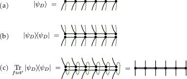
Figure 2: Obtaining an MPO description of $\operatorname*{Tr}_{\mathrm{fict}}{|{\psi_{D}}\rangle\langle{\psi_{D}}|}$ from the MPS ${|{\psi_{D}}\rangle}$. (a) The MPS ${|{\psi_{D}}\rangle}$. Each leg is represented by two legs, where the solid leg corresponds to the original local Hilbert space and the dashed leg to the fictitious Hilbert space. (b) The TN representation of ${|{\psi_{D}}\rangle\langle{\psi_{D}}|}$. (c) To calculate $\operatorname*{Tr}_{\mathrm{fict}}{|{\psi_{D}}\rangle\langle{\psi_{D}}|}$ we contract the fictitious legs, leading to an MPO with bond dimension $D^{2}$.

We conclude the discussion by noting that vectorization also maps super-operators to operators. Indeed, for every super operator $\mathcal{F}$ there is a unique $F\in L(\mathbbm{H}\otimes\mathbbm{H})$ that satisfies

$$|\mathcal{F}(X)\rangle\!\rangle\stackrel{{\scriptstyle\mathrm{def}}}{{=}}F|X\rangle\!\rangle.$$

This map respects the notion of adjoints in the sense that $\mathcal{F}\mapsto F$ iff $\mathcal{F}^{*}\mapsto F^{\dagger}$, and so a self-adjoint super Hamiltonian $\mathcal{H}$ is mapped to an hermitian Hamiltonian $H$. It is easy to verify that if $\mathcal{F}$ is the superoperator $\mathcal{F}(X)\stackrel{{\scriptstyle\mathrm{def}}}{{=}}A\cdot X\cdot B$, then its vectorization is the operator $F=A\otimes B^{T}$. Using this formula it is clear that a $k$-body super-operator maps to a $2k$-body operator. For example, the super Hamiltonian (19) from Theorem 3.1 is mapped to the Hamiltonian

$$H=-\sum_{j}\left[\sqrt{c_{j}c_{\pi(j)}}L_{j}\otimes L_{j}^{*}-\frac{c_{j}}{2}\big{(}L_{j}^{\dagger}L_{j}\otimes\mathbbm{1}+\mathbbm{1}\otimes(L_{j}^{\dagger}L_{j})^{T}\big{)}\right],$$

and a similar expression arises for the super Hamiltonian from Theorem 3.2.

3.2.2 Area laws for steady states

In this subsection we use the notation $\tilde{O}(X)$ for $\operatorname{O}\bigl{(}X\cdot\mathrm{poly}(\log X)\bigr{)}$. Our first result will be an area law for 1D Lindbladians that satisfy the requirements of Theorem 3.1. These map to geometrically local 1D super Hamiltonians, for which we will use the following result:

Theorem 3.7 (Taken from Refs. [29, 45])

Let $\Lambda$ be a 1D lattice of sites with local dimension $d$. Let $H=\sum_{i}h_{i}$ be a nearest neighbours Hamiltonian with a spectral gap $\gamma>0$ and a unique ground state ${|{\Omega}\rangle}$. Assume, in addition, that ${\|h_{i}\|}\leq J$ for every $i$, where $J$ is some energy scale. Then the entanglement entropy of ${|{\Omega}\rangle}$ with respect to any bi-partition satisfies $S_{E}=\tilde{O}\big{(}\frac{\log^{3}(d)}{\gamma/J}\big{)}$. Moreover, there is a matrix product state (MPS) ${|{\psi_{D}}\rangle}$ of sublinear bond dimension $D=e^{\tilde{O}(\log^{3/4}n/(\gamma/J)^{1/4})}$ such that ${\|{|{\Omega}\rangle}-{|{\psi_{D}}\rangle}\|}\leq\frac{1}{\mathrm{poly}(n)}$, and such MPS can be found efficiently on a classical computer.

Using the above theorem together with Lemma 3.6 and Theorem 3.1, we immediately obtain the following corollary

Corollary 3.8

Let $\mathcal{L}$ be a geometrically local $2$-body Lindbladian defined on a 1D lattice of local dimension $d$ that satisfies the requirements of Theorem 3.1. Assume in addition that $\mathcal{L}$ has a gap $\gamma>0$, a unique steady state, and that $|c_{j}|\leq J$ for all $j$. Then:

1. $\sqrt{\sigma}$ satisfies an area law for the operator-space entanglement entropy [48], that is, for any cut in the 1D lattice into $\Lambda=L\cup R$ the entanglement entropy of $|\sqrt{\sigma}\rangle\!\rangle$ between the two parts satisfies

   $$S(L)_{\rho}=\tilde{O}\big{(}\frac{\log^{3}(d)}{\gamma/J}\big{)}.$$ (25)

2. $\sigma$ satisfies an area-law for the mutual information. Specifically, for any cut in the 1D lattice, the mutual information between the two sides satisfies

   $$I(L:R)_{\sigma}=\tilde{O}\big{(}\frac{\log^{3}(d)}{\gamma/J}\big{)}.$$ (26)

3. There is a matrix product operator (MPO) $\Psi_{D}$ with bond dimension $D=e^{\tilde{O}(\log^{3/4}n/(\gamma/J)^{1/4})}$ such that ${\|\sigma-\Psi_{D}\|}_{1}\leq\frac{1}{\mathrm{poly}(n)}$. Moreover, a similar approximating MPO for $\sigma$ can be found efficiently on a classical computer.

For the next result, we will use the main result of Ref. [30] adapted to the $2$-local settings with exponentially decaying interactions.

Theorem 3.9 (Taken from Ref. [30])

Let $\Lambda$ a 1D lattice of sites with local dimension $d$. Let $H=\sum_{i,j}h_{ij}+\sum_{i}h_{i}$ be a $2$-body Hamiltonian defined on $\Lambda$, and suppose that there exist a constant $J$ such that ${\|h_{ij}\|}\leq\frac{J}{r_{ij}^{\alpha}},\;{\|h_{i}\|}\leq J$, and that $H$ has a spectral gap $\gamma>0$ and a unique ground state ${|{\Omega}\rangle}$. Then the entanglement entropy of ${|{\Omega}\rangle}$ with respect to any cut in the 1D grid satisfies

$$S_{E}=\tilde{O}\left(\log^{2}d\left(\frac{\log d}{\gamma/J}\right)^{1+\frac{2}{\alpha-2}}\right).$$

Moreover, there is a MPS ${|{\psi_{D}}\rangle}$ of bond dimension $D=e^{\operatorname{O}\bigl{(}\log^{5/2}(n)\bigr{)}}$ such that ${\|{|{\Omega}\rangle}-{|{\psi_{D}}\rangle}\|}\leq\frac{1}{\mathrm{poly}(n)}$.

It should be noted that Theorem 3.9 can be restated for 1D $k$-local Hamiltonians and still give the same entropy bound — see Appendix B in Ref. [30]. Using the above theorem, together with Lemma 3.6 and Corollary 3.5, we can choose an appropriate $B$ for which ${\|\mathcal{H}_{ab}\|}\leq B/|a-b|^{\alpha}$ for any $P_{a},P_{b}$ for some $\alpha>4$. This implies the following corollary:

Corollary 3.10

Let $\mathcal{L}$ be a geometrically local $2$-body Lindbladian defined on a $1D$ lattice that satisfies the requirements of Theorem 3.2, with a spectral gap $\gamma>0$ and a steady state $\sigma$. Assume also that the smallest non-vanishing eigenvalue of $C\cdot C^{*}$ is $\lambda_{\mathrm{min}}=\operatorname{\Omega}\bigl{(}1\bigr{)}$. Then

1. $\sqrt{\sigma}$ satisfies an area law for the operator-space entanglement entropy [48]. That is, for any cut in the 1D lattice into $\Lambda=L\cup R$ the entanglement entropy of $|\sqrt{\sigma}\rangle\!\rangle$ between the two parts satisfies

   $$S(L)_{\rho}=\tilde{O}\left(\log^{2}d\left(\frac{\log d}{\gamma/J}\right)^{2}\right).$$ (27)

2. $\sigma$ satisfies an area-law for the mutual information. Specifically, for any cut in the 1D lattice, the mutual information between the two sides satisfies

   $$I(L:R)_{\sigma}=\tilde{O}\left(\log^{2}d\left(\frac{\log(d}{\gamma/J}\right)^{2}\right).$$ (28)

3. There is a matrix product operator (MPO) $\Psi_{D}$ with bond dimension $D=e^{\operatorname{O}\bigl{(}\log^{5/2}(n)\bigr{)}}$ such that ${\|\sigma-\Psi_{D}\|}_{1}\leq\frac{1}{\mathrm{poly}(n)}$.

We finish this part by noting that there are many more applications of the theorems in subsection 3.1 which we did not address. For example:

1. One can import other ground state area-law results to the Linbladian settings, including results for 2D and higher dimensions such as those given in Refs.  [5, 7, 8, 9, 11].

2. One can use the results in Refs. [50, 46] to show exponential decay of correlations for $|\sqrt{\sigma}\rangle\!\rangle$, which implies the same for $\sigma$ using Eq. (23). This was already shown in Ref. [18] (see Theorem 9 in the paper), so we omit the details. Notice that our result are implied for any such Lindbladian without assuming local uniqueness (see regular Lindbladians in Ref. [18]).

3. One can demonstrate a gap in the Lindbladian by demonstrating a gap in the super-Hamiltonian instead. As the former task is somewhat challenging, the latter has been discussed more frequently in the literature. Below we will exemplify this by using the finite-size criteria from Ref. [33] to demonstrate a gap for a family of Lindbladians (see the proof of Claim 4.1, bullet 4 for details). We remark that this type of work has been also done in Ref. [17].

3.3 Proofs of Theorems 3.1, 3.2

In this section we give the proofs of our main results, Theorems 3.1, 3.2. The two proofs follow the same outline: Examining the continuous family of superoperators $\mathcal{L}_{x}\stackrel{{\scriptstyle\mathrm{def}}}{{=}}\Gamma_{s}^{-x}\circ\mathcal{L}\circ\Gamma_{s}^{x}$, we would like to show that it obeys some notion of locality at $x=1/2$. In fact, we will show that it is local for all $x\in\mathbbm{R}$. By definition, $\mathcal{L}_{0}=\mathcal{L}$, and by the QDB condition (12), $\mathcal{L}_{1}=\Gamma_{s}^{-1}\circ\mathcal{L}\circ\Gamma_{s}=\mathcal{L}^{*}$, both of which are local. To prove locality for all other $x\in\mathbbm{R}$ we use the modular basis (see Corollary 2.9). We will show that $\mathcal{L}_{x}$ remains diagonal in the modular basis for every $x$. Then, we will use Theorem 2.2 to establish a connection between the local representation of $\mathcal{L}$ and the modular basis. Finally, we will employ the fact that $\mathcal{L}_{1}$ is local to argue that it must remain local for all $x\in\mathbbm{R}$.

Let us then begin by proving that $\mathcal{L}_{x}$ remains diagonal in the modular basis.

Lemma 3.11

(Adaptation of Lemma 7 from Ref. [20])  
Let $\mathcal{L}$ satisfy the quantum detailed-balance condition with respect to $s\in[0,1/2)\cup(1/2,1]$. Then for every $x\in\mathbbm{R}$, the superoperator $\Gamma_{s}^{-x}\circ\mathcal{L}\circ\Gamma_{s}^{x}$ is diagonal in the modular basis, and is given by

$$(\Gamma_{s}^{-x}\circ\mathcal{L}\circ\Gamma_{s}^{x})(A) =\sum_{\alpha\in I}\gamma_{\alpha}e^{-\omega_{\alpha}/2}\Big{(}e^{x\omega_{\alpha}}S_{\alpha}AS_{\alpha}^{\dagger}-\frac{1}{2}\big{\{}S_{\alpha}^{\dagger}S_{\alpha},A\big{\}}\Big{)}.$$

Note: the above formula is identical to the formula for $\mathcal{L}$ in Theorem 2.10, except for the $e^{x\omega_{\alpha}}$ factor in front of the $S_{\alpha}AS_{\alpha}^{\dagger}$ term.

• Recall that $\Gamma_{s}^{x}(A)=\sigma^{x(1-s)}A\sigma^{xs}$. We consider the terms $S_{\alpha}AS_{\alpha}^{\dagger}$ and $\{S_{\alpha}^{\dagger}S_{\alpha},A\}$ separately. The conjugation of $S_{\alpha}AS_{\alpha}^{\dagger}$ gives

  $$\big{(}\Gamma_{s}^{-x}\circ(A\mapsto S_{\alpha}AS_{\alpha}^{\dagger})\circ\Gamma_{s}^{x}\big{)}(A) =\Gamma_{s}^{-x}\big{(}S_{\alpha}\Gamma_{s}^{x}(A)S_{\alpha}^{\dagger}\big{)}=\sigma^{-x(1-s)}S_{\alpha}\sigma^{x(1-s)}A\sigma^{xs}S_{\alpha}^{\dagger}\sigma^{-xs}.$$ (29)

  Recalling that

  $$\sigma^{-x(1-s)}S_{\alpha}\sigma^{x(1-s)} =\Delta_{\sigma}^{-x(1-s)}(S_{\alpha})=e^{x(1-s)\omega_{\alpha}}S_{\alpha},$$

  $$\sigma^{xs}S^{\dagger}_{\alpha}\sigma^{-xs} =\Delta_{\sigma}^{xs}(S^{\dagger}_{\alpha})=e^{xs\omega_{\alpha}}S^{\dagger}_{\alpha},$$

  we find that, overall, $\big{(}\Gamma_{s}^{-x}\circ(A\mapsto S_{\alpha}AS_{\alpha}^{\dagger})\circ\Gamma_{s}^{x}\big{)}(A)=e^{x\omega_{\alpha}}S_{\alpha}AS_{\alpha}^{\dagger}$.

  For the the anti-commutator conjugation, we have:

  $$\big{(}\Gamma_{s}^{-x}\circ(A\mapsto\{S^{\dagger}_{\alpha}S_{\alpha},A\})\circ\Gamma_{s}^{x}\big{)}(A) =\Gamma_{s}^{-x}\big{(}\{S_{\alpha}^{\dagger}S_{\alpha},\Gamma_{s}^{x}(A)\}\big{)}=\sigma^{-x(1-s)}\{S_{\alpha}^{\dagger}S_{\alpha},\sigma^{x(1-s)}A\sigma^{xs}\}\sigma^{-xs}$$

  $$=\sigma^{-x(1-s)}S_{\alpha}^{\dagger}S_{\alpha}\sigma^{x(1-s)}A+A\sigma^{xs}S_{\alpha}^{\dagger}S_{\alpha}\sigma^{-xs}=\{S_{\alpha}^{\dagger}S_{\alpha},A\},$$

  where in the last equality we used the fact that for every $t$,

  $$\sigma^{t}S_{\alpha}^{\dagger}S_{\alpha}\sigma^{-t}=\sigma^{t}S_{\alpha}^{\dagger}\sigma^{-t}\sigma^{t}S_{\alpha}\sigma^{-t}=\Delta_{\sigma}^{t}(S_{\alpha})\Delta_{\sigma}^{t}(S^{\dagger}_{\alpha})=e^{-t\omega_{\alpha}}S_{\alpha}e^{t\omega_{\alpha}}S^{\dagger}_{\alpha},=S_{\alpha}S^{\dagger}_{\alpha}.$$

   

With Lemma 3.11 at hand, we turn to the proof of Theorem 3.1.

3.3.1 Proof of Theorem 3.1

By assumption, $\mathcal{L}$ is given by

$$\mathcal{L}(A)=\sum_{j}c_{j}\big{(}L_{j}AL_{j}^{\dagger}-\frac{1}{2}\{L_{j}^{\dagger}L_{j},A\}\big{)},$$

but in addition, by the QDB condition and Theorem 2.10, it is given by a canonical form

$$\mathcal{L}(A)=\sum_{\alpha\in I}\gamma_{\alpha}e^{-\omega_{\alpha}/2}\Big{(}S_{\alpha}AS_{\alpha}^{\dagger}-\frac{1}{2}\big{\{}S_{\alpha}^{\dagger}S_{\alpha},A\big{\}}\Big{)}.$$

Therefore, by Theorem 2.2, there must be a unitary $U_{\alpha,j}$ that connects these two bases, i.e.,

$$\sqrt{\gamma_{\alpha}}e^{-\omega_{\alpha}/4}S_{\alpha}=\sum_{j}U_{\alpha,j}\sqrt{c_{j}}L_{j}.$$ (30)

Let us now consider the superoperator $\mathcal{L}_{x}\stackrel{{\scriptstyle\mathrm{def}}}{{=}}\Gamma_{s}^{-x}\circ\mathcal{L}\circ\Gamma_{s}^{x}$. By Lemma 3.11, it is given by

$$\mathcal{L}_{x}(A)=\sum_{\alpha\in I}\gamma_{\alpha}e^{-\omega_{\alpha}/2}\Big{(}e^{x\omega_{\alpha}}S_{\alpha}AS_{\alpha}^{\dagger}-\frac{1}{2}\big{\{}S_{\alpha}^{\dagger}S_{\alpha},A\big{\}}\Big{)},$$

and therefore by Eq. (30), it can also be written in terms of the $L_{j}$ basis as

$$\mathcal{L}_{x}(A) =\sum_{\alpha,j,j^{\prime}}e^{x\omega_{\alpha}}U_{\alpha,j}U_{\alpha,j^{\prime}}^{*}\sqrt{c_{j}c_{j^{\prime}}}L_{j}AL_{j^{\prime}}^{\dagger}-\frac{1}{2}\sum_{j}c_{j}\big{\{}L_{j}^{\dagger}L_{j},A\}.$$

Note that the anti-commutator term remained unchanged. To analyze the first term, we define the matrix $B$

$$B_{j^{\prime}j}\stackrel{{\scriptstyle\mathrm{def}}}{{=}}\sum_{\alpha}e^{\omega_{\alpha}}U_{\alpha,j}U_{\alpha,j^{\prime}}^{*}.$$

Note that $B=U^{\dagger}\cdot\operatorname{diag}(\{e^{\omega_{\alpha}}\})\cdot U$, and therefore $B^{x}=U^{\dagger}\cdot\operatorname{diag}(\{e^{x\omega_{\alpha}}\})\cdot U$, hence

$$\mathcal{L}_{x}(A)=\sum_{j,j^{\prime}}B^{x}_{j^{\prime}j}\sqrt{c_{j^{\prime}}c_{j}}L_{j}AL^{\dagger}_{j^{\prime}}-\frac{1}{2}\sum_{j}c_{j}\big{\{}L_{j}^{\dagger}L_{j},A\}.$$ (31)

To prove the locality of $\mathcal{L}_{x}$, we would like to show that $B_{j^{\prime}j}^{x}\propto\delta_{jj^{\prime}}$, , i.e., that $B^{x}$ is diagonal, for at least one $\tilde{x}\neq 0$, which will then imply that it also diagonal for all $x\in\mathbbm{R}$. This is done using the QDB condition (12), which will let show diagonality for $\tilde{x}=1$. The QDB condition is equivalent to

$$\mathcal{L}_{1}(A)=\mathcal{L}^{*}(A)=\sum_{j}c_{j}\big{(}L^{\dagger}_{j}AL_{j}-\frac{1}{2}\{L_{j}^{\dagger}L_{j},A\}\big{)}.$$

Comparing to Eq. (31) gives the condition

$$\sum_{j^{\prime}j}B_{j^{\prime}j}\sqrt{c_{j^{\prime}}c_{j}}L_{j}AL^{\dagger}_{j^{\prime}}=\sum_{j}c_{j}L^{\dagger}_{j}AL_{j}=\sum_{j}c_{\pi(j)}L_{j}AL_{j}^{\dagger},$$

where in the last equality we used the definition of $\pi(j)$, $L_{\pi(j)}=L^{\dagger}_{j}$. Let us now use the assumption that the jump operators $\{L_{j}\}$ are linearly independent. This implies that the coefficients of $L_{j}AL_{j^{\prime}}^{\dagger}$ on both sides of the equation should be identical, and therefore,

$$B_{j^{\prime}j}\sqrt{c_{j^{\prime}}c_{j}}=c_{\pi(j)}\delta_{j^{\prime}j}.$$

Using the assumption that $c_{j}>0$, we conclude that

$$B_{j^{\prime}j}=\frac{c_{\pi(j)}}{c_{j}}\delta_{j^{\prime}j},$$

and therefore,

$$\mathcal{L}_{x}(A)=\sum_{j}\Big{(}c_{\pi(j)}^{x}c^{1-x}_{j}L_{j}AL^{\dagger}_{j}-\frac{c_{j}}{2}\big{\{}L_{j}^{\dagger}L_{j},A\}\Big{)}.$$ (32)

Substituting $x=1/2$ concludes the proof.  

3.3.2 Proof of Theorem 3.2

As in the proof of Theorem 3.1, we show the locality of $\mathcal{H}$ using its modular basis representation. We start by noting that all the modular basis elements $S_{\alpha}$ that appear in $\mathcal{L}$ in (15) (those with $\gamma_{\alpha}>0$) can be unitarily expressed by the orthonormal basis $\{P_{a}\}$. Indeed, starting from the jump operators representation in Eq. (16), we conclude from Theorem 2.2 that whenever $\gamma_{\alpha}>0$, $S_{\alpha}$ can be written in terms of the jump operators $L_{j}$. But as $L_{j}$ can be expanded in terms of the local $\{P_{a}\}$ operators, it follows that this also holds for $S_{\alpha}$ as well. Finally, by the orthonormality of both sets of operators, we conclude that they are unitarily related: There exists a unitary $U_{a\alpha}$, where $\alpha$ runs over all the indices $\alpha$ for which $\gamma_{\alpha}>0$, such that

$$S_{\alpha}=\sum_{a}U_{a\alpha}P_{a}.$$ (33)

Plugging the expansion (33) into the canonical form (15) gives

$$\mathcal{L}(\rho)=\sum_{a,b,\alpha}U_{a\alpha}\gamma_{\alpha}e^{-\omega_{\alpha}/2}U_{b\alpha}^{*}\big{(}P_{a}\rho P_{b}-\frac{1}{2}\{P_{b}P_{a},\rho\}\big{)}.$$

Comparing with Eq. (21), we use the fact that once an orthonormal basis is fixed, the coefficients of the Lindbladians are also fixed (see, e.g., Theorem 2.2 in Ref. [43]). Therefore,

$$C =UDU^{\dagger}, D \stackrel{{\scriptstyle\mathrm{def}}}{{=}}\operatorname{diag}\big{(}\{\gamma_{\alpha}e^{-\omega_{\alpha}/2}\}\big{)},$$

where $C$ is the coefficient matrix of the expansion of $\mathcal{L}$ in terms of the $\{P_{a}\}$ operators (Eq. (21)).

We now examine the superoperator $\mathcal{L}_{x}\stackrel{{\scriptstyle\mathrm{def}}}{{=}}\Gamma_{s}^{-x}\circ\mathcal{L}\circ\Gamma_{s}^{x}$, which by Lemma 3.11 is given by

$$\mathcal{L}_{x}(\rho)=\sum_{\alpha\in I}\gamma_{\alpha}e^{\omega_{\alpha}(x-1/2)}S_{\alpha}\rho S_{\alpha}^{\dagger}-\frac{1}{2}\sum_{\alpha\in I}\gamma_{\alpha}e^{-\omega_{\alpha}/2}\big{\{}S_{\alpha}^{\dagger}S_{\alpha},\rho\big{\}}.$$

Using Eq. (33), we can rewrite it in terms of the $\{P_{a}\}$ operators as

$$\mathcal{L}_{x}(\rho) =\sum_{a,b}C_{ab}(x)P_{a}\rho P_{b}-\frac{1}{2}\sum_{a,b}C_{ab}\{P_{b}P_{a},\rho\},$$ (34)

where we defined

$$C(x)\stackrel{{\scriptstyle\mathrm{def}}}{{=}}U\cdot\operatorname{diag}\left(\{\gamma_{\alpha}e^{\omega_{\alpha}(x-1/2)}\}\right)\cdot U^{\dagger}.$$ (35)

Note that $C(x)$ commutes with $C(x^{\prime})$ for any $x,x^{\prime}$, as they are both diagonalized by $U$. As in the proof of the previous theorem, we know that $C(x)$ is local for $x=0$ and we would like to prove locality for every $x\in\mathbbm{R}$. We do this by using the QDB condition to show that also the $\tilde{x}=1$ is local, and by showing that any other $x\in\mathbbm{R}$, $C(x)$ is a simple function of $C(0)$ and $C(1)$.

Consider then the $\tilde{x}=1$ point. By the QDB condition (12), it follows that

$$\mathcal{L}_{1}=\Gamma_{s}^{-1}\circ\mathcal{L}\circ\Gamma_{s}=\mathcal{L}^{*}=\sum_{a,b}C^{*}_{ab}\big{(}P_{a}\rho P_{b}-\frac{1}{2}\{P_{a}P_{b},\rho\}\big{)}.$$

Comparing it to Eq. (34) and using the fact that $C$ is Hermitian, we conclude that $C(1)=C^{*}$, and therefore, $C^{*}$ commutes with $C=C(0)$. Finally, a simple algebra shows that

$$C^{1-x}\cdot(C^{*})^{x} =U\cdot\operatorname{diag}\big{(}\{\gamma^{1-x}_{\alpha}\cdot e^{-\omega_{\alpha}(1-x)/2}\}\big{)}\cdot\operatorname{diag}\big{(}\{\gamma^{x}_{\alpha}\cdot e^{x\omega_{\alpha}/2}\}\big{)}\cdot U^{\dagger}$$

$$=U\cdot\operatorname{diag}\big{(}\{\gamma_{\alpha}e^{\omega_{\alpha}(x-1/2)}\}\big{)}\cdot U^{\dagger}=C(x).$$

which can also be written as $C(x)=C^{1-x}(0)\cdot C^{x}(1)$. Substituting $x=1/2$, and using Eq. (34) proves the theorem.

4 Examples

In this section, we describe two exactly solvable models whose dynamics is governed by a Lindbladian satisfying, respectively, the requirements of Theorem 3.1 and Theorem 3.2 from section 3. In subsection 4.1 we describe classical Metropolis-based dynamics that satisfies the conditions of Theorem 3.1, and in subsection 4.2 we describe a family of quadratic fermion models that satisfy the conditions of Theorem 3.2. For both models, we prove detailed balance, unique steady-state and constant spectral gap. As the models are exactly solvable, we give explicit expressions for their super Hamiltonians, which are derived independently of the results of subsection 3.1.

4.1 Model for Theorem 3.1: Classical-like Lindbladians

Here we describe a system that obeys the requirements of Theorem 3.1. First, we specify the steady state, which is the Gibbs state of a classical Hamiltonian, and then write the corresponding Lindbladian that annihilates it; this Lindbladian gives rise to classical thermalization dynamics of the diagonal elements of the density matrix, while dephasing away the off-diagonal elements. The full proofs are given in Appendix B.

We consider a 1D lattice with periodic boundary conditions, where a single qubit occupies each site. Intuitively, we think of each site $i$ as being able to hold a particle (e.g., a fermion or a hard core boson) with some energy $\epsilon_{i}$, or being empty. The state of the system is then described by a binary string ${\underline{x}}=(x_{1},\ldots,x_{n})\in\{0,1\}^{n}$, where $x_{i}$ determines the occupation of the $i$th site (either $0$ or $1$). To achieve a non-trivial Gibbs state, we define a constant interaction $u$ acting between nearest neighbours, which is non-zero if an only if both neighbouring sites are simultaneously occupied by a particle. To write down the Hamiltonian of the system, we let $n_{i}\stackrel{{\scriptstyle\mathrm{def}}}{{=}}\frac{1}{2}(\mathbbm{1}-Z_{i})={|{1}\rangle\langle{1}|}_{i}$ denote occupation number operator at site $i$, and let $\mu>0$ denote a chemical potential. Our Hamiltonian is then given by

$$H\stackrel{{\scriptstyle\mathrm{def}}}{{=}}\sum_{i=1}^{n}(\epsilon_{i}-\mu)n_{i}+u\sum_{i=1}^{n}n_{i}\cdot n_{i+1}.$$

This is a classical Hamiltonian that is diagonal in the computational basis ${|{{\underline{x}}}\rangle}={|{x_{1}}\rangle}\otimes\ldots\otimes{|{x_{n}}\rangle}$, and its Gibbs state is

$$\sigma =\frac{1}{Z}\sum_{{\underline{x}}\in\{0,1\}^{n}}e^{-\beta E_{x}}{|{{\underline{x}}}\rangle\langle{{\underline{x}}}|},$$ (36)

$$E_{\underline{x}} \stackrel{{\scriptstyle\mathrm{def}}}{{=}}\sum_{i=1}^{n}(\epsilon_{i}-\mu)x_{i}+u\sum_{i=1}^{n}x_{i}x_{i+1},$$ (37)

$$Z \stackrel{{\scriptstyle\mathrm{def}}}{{=}}\sum_{{\underline{x}}\in\{0,1\}^{n}}e^{-\beta E_{x}}.$$ (38)

We now introduce a Lindbladian that drives the system into $\sigma$. It is a geometrically $3$-local Lindbladian that is given by

$$\mathcal{L}\stackrel{{\scriptstyle\mathrm{def}}}{{=}}\sum_{k,b}\gamma_{k,b}\mathcal{L}_{k,b},$$ (39)

where $k\in\{1,\ldots,n\}$, $b\in\{0,1,2\}$ and $\{\gamma_{k,b}\}$ are some positive (possibly random) $O(1)$ constants. For each $k,b$, the superoperator $\mathcal{L}_{k,b}$ act locally on qubits $k-1,k,k+1$ and is defined by:

$$\mathcal{L}_{k,b}(\rho)\stackrel{{\scriptstyle\mathrm{def}}}{{=}}e^{-\beta\omega_{k,b}/2}\left(L_{k,b}\rho L_{k,b}^{\dagger}-\frac{1}{2}\{L_{k,b}^{\dagger}L_{k,b},\rho\}\right)+e^{\beta\omega_{k,b}/2}\left(L_{k,b}^{\dagger}\rho L_{k,b}-\frac{1}{2}\left\{L_{k,b}L_{k,b}^{\dagger},\rho\right\}\right),$$ (40)

where $\omega_{k,b}\stackrel{{\scriptstyle\mathrm{def}}}{{=}}-(\epsilon_{k}-\mu)-u\cdot b$ and $L_{k,b}$ are $3$-local jump operators given by

$$L_{k,b}\stackrel{{\scriptstyle\mathrm{def}}}{{=}}\sigma^{-}_{k}\otimes\Pi^{b}_{k-1,k+1}\otimes\mathbbm{1}_{\mathrm{rest}}.$$ (41)

Above, $\sigma^{-}_{k}\stackrel{{\scriptstyle\mathrm{def}}}{{=}}{|{0}\rangle\langle{1}|}_{k}$ is the “annihilation operator” on site $k$, and $\Pi^{b}_{k-1,k+1}$ is the projector onto the subspace in which the sum of the occupation numbers of sites $k-1$ and $k+1$ is equal to $b$ (for $b\in\{0,1,2\}$).

We will now show that $\sigma$ is the unique steady state of $\mathcal{L}$, and that $\mathcal{L}$ is gapped and satisfies QDB. The key is to show explicitly that the representation of $\mathcal{L}$ in Eq. (40) is the canonical representation, from which it will follow by Theorem 2.10 that $\mathcal{L}$ satisfies QDB with respect to $\sigma$, and therefore it is a steady state of $\mathcal{L}$. Formally, we claim:

Claim 4.1

The following properties hold for the Lindbladian $\mathcal{L}$ defined in (39):

1. The jump operators $\{L_{k,b},L_{k,b}^{\dagger}\}$ are taken from a modular basis (up to normalization), and so $\mathcal{L}$ is given in the canoniconical representation.

2. $\mathcal{L}_{k,b}$ satisfy local detailed-balance with respect to $\sigma$,

   $$\mathcal{L}_{k,b}\circ\Gamma_{s}=\Gamma_{s}\circ\mathcal{L}_{k,b}^{*}\hskip 28.45274pt\forall s\in[0,1].$$

3. If $\gamma_{k,b}>0$, then $\mathcal{L}$ has a unique steady state $\sigma$ defined in Eq. (36).

4. If $\gamma_{k,b}\geq\alpha>0$ and $\epsilon_{k}-\mu,u=\operatorname{O}\bigl{(}1\bigr{)}$, then $\mathcal{L}$ is gapped with $\operatorname{gap}{\mathcal{L}}=\operatorname{\Omega}\bigl{(}\alpha\bigr{)}$.

• To show that $\mathcal{L}$ is given in the canonical form, we will show that $\{L_{k,b}\}$ is a proper modular basis with well-defined Bohr frequencies given by $\beta\omega_{kb}$. First, it is easy to see that $\{L_{k,b}\}$ are orthogonal and traceless. To see that they have well-defined Bohr frequencies, we need to show that $\Delta_{\sigma}(L_{k,b})=e^{-\omega_{k,b}}L_{k,b}$, where $\Delta_{\sigma}(L_{k,b})=\sigma L_{k,b}\sigma^{-1}$. By Eq. (36),

  $$\Delta_{\sigma}(L_{k,b})=\sum_{{\underline{x}}^{\prime},{\underline{x}}}e^{-\beta(E_{{\underline{x}}^{\prime}}-E_{{\underline{x}}})}{|{{\underline{x}}^{\prime}}\rangle\langle{{\underline{x}}^{\prime}}|}L_{k,b}{|{{\underline{x}}}\rangle\langle{{\underline{x}}}|}.$$ (42)

  However, by the definition of $L_{k,b}$,

  $${\langle{{\underline{x}}^{\prime}}|}L_{k,b}{|{{\underline{x}}}\rangle}=\begin{cases}1,&x_{k}=1,\;x^{\prime}_{k}=0,\;x_{i}=x^{\prime}_{i}\;\mathrm{forall}\;i\neq k,\;\mathrm{and}\;x_{k-1}+x_{k+1}=b\\ 0,&\mathrm{otherwise}.\end{cases}$$ (43)

  Therefore, whenever ${\langle{{\underline{x}}^{\prime}}|}L_{k,b}{|{{\underline{x}}}\rangle}\neq 0$,

  $$E_{x^{\prime}}-E_{x}=\sum_{i=1}^{n}(\epsilon_{i}-\mu)({x^{\prime}}_{i}-x_{i})+u\sum_{i=1}^{n}({x^{\prime}}_{i}{x^{\prime}}_{i+1}-x_{i}x_{i+1})=-(\epsilon_{k}-\mu)-ub=\omega_{k,b}.$$

  Plugging this into Eq. (42), we get

  $$\Delta_{\sigma}(L_{k,b})=e^{-\beta\omega_{k,b}}\sum_{{\underline{x}}^{\prime},{\underline{x}}}{|{{\underline{x}}^{\prime}}\rangle\langle{{\underline{x}}^{\prime}}|}L_{k,b}{|{{\underline{x}}}\rangle\langle{{\underline{x}}}|}=e^{-\beta\omega_{k,b}}L_{k,b}.$$

  A similar calculation shows that $\Delta_{\sigma}(L^{\dagger}_{k,b})=e^{\beta\omega_{k,b}}L^{\dagger}_{k,b}$.

  Using Theorem 2.10 it follows that for every $k,b$, $\mathcal{L}_{k,b}$ satisfies the QDB condition for $s\in[0,1/2)\cup(1/2,1]$ (and therefore also for $s=1/2$) with respect to $\sigma$, i.e., $\Gamma_{s}\circ\mathcal{L}_{k,b}=\mathcal{L}_{k,b}^{*}\circ\Gamma_{s}$. As shown in the end of subsection 2.3, this implies that $\sigma$ is annihilated by $\mathcal{L}_{k,b}$. Therefore, $\sigma$ is a fixed point of $\mathcal{L}$, and, moreover, it is a “frustration-free” Lindbladian.

  Showing uniqueness and gap (bullets 3,4) are technically more involved, requiring the use of Knabe and Perron-Frobenious Theorems, and are therefore deferred to Appendix B.

   

Using the claim above, specifically bullet 2, the superoperator $\mathcal{H}_{k,b}\stackrel{{\scriptstyle\mathrm{def}}}{{=}}\Gamma_{s}^{-1/2}\circ\mathcal{L}_{k,b}\circ\Gamma_{s}^{1/2}$ is self-adjoint and annahilates $\sqrt{\sigma}$. Then, using bullet 1, we can apply Lemma 3.11 to $\mathcal{L}_{k,b}$ given in Eq. (40) to get

$$\mathcal{H}_{k,b}=-\left(L_{k,b}\rho L_{k,b}^{\dagger}+L_{k,b}^{\dagger}\rho L_{k,b}-\frac{e^{-\beta\omega_{k,b}/2}}{2}\{L_{k,b}^{\dagger}L_{k,b},\rho\}-\frac{e^{\beta\omega_{k,b}/2}}{2}\left\{L_{k,b}L_{k,b}^{\dagger},\rho\right\}.\right)$$ (44)

Consequently, $\mathcal{H}=\sum_{k,b}\gamma_{k,b}\mathcal{H}_{k,b}$ is a frustration-free local super-Hamiltonian. While the locality of $\mathcal{H}$ is guaranteed by Theorem 3.1, frustration-freeness is an extra feature that follows from that fact that every $\mathcal{L}_{k,b}$ is locally QDB. This allows us to use tools of frustration-free Hamiltonians to study $\mathcal{H}$ and $\mathcal{L}$. For example, we prove bullet 4 of Claim 4.1 using techniques from Refs.  [33, 34, 51]. We believe this method may be beneficial for physicists when investigating detailed-balance semigroups and specifically Davies generators [44, 19, 32]. As a final remark, we mention that this could be extended to more complicated Lindblad operators, higher dimensional lattices, and other degrees of freedom (e.g., bosons with a larger finite set of allowed occupancies per site or qudits).

4.2 Model for Theorem 3.2: Quadratic fermionic Lindbladians

We now describe a family of models that satisfies the requirements of Theorem 3.2. The models consist of free spinless fermions on a lattice, coupled to two particle reservoirs, one with infinitely high chemical potential and one with an infinitely low chemical potential. The high chemical potential reservoir emits particles into the system, and the low chemical potential reservoir takes particles out of the system. The reservoirs are assumed to be large and Markovian, such that they can be integrated out and result in a dissipative Lindblad evolution of the lattice. A physical realization of such settings can be found in, e.g., Section 3 of Ref. [52]; such Lindbladians can be used for the dissipative generation of topologically nontrivial states  [53, 54].

The models are governed by quadratic Lindbladians of the form [55, 52, 56]

$$\mathcal{L}(\rho)=\sum_{i,j}\gamma^{\mathrm{in}}_{ij}\left(a_{i}^{\dagger}\rho a_{j}-\frac{1}{2}\{a_{j}a_{i}^{\dagger},\rho\}\right)+\gamma^{\mathrm{out}}_{ji}\left(a_{i}\rho a_{j}^{\dagger}-\frac{1}{2}\{a_{j}^{\dagger}a_{i},\rho\}\right),$$ (45)

$a_{i}$, $a_{i}^{\dagger}$ are, respectively fermionic annihilation and creation operators obeying the standard anticommutation relations, and where $\gamma^{\mathrm{in}},\gamma^{\mathrm{out}}$ are positive semi definite matrices with eigenvalues $d_{k}^{\mathrm{in}},d_{k}^{\mathrm{out}}$, respectively. Physically, $\gamma^{\mathrm{in}}$ ($\gamma^{\mathrm{out}}$) is responsible for the absorption (emission) of particles from (into) the environment. This model can be seen as a special case of a scenario which is treated by Theorem 3.2. However, we find it more illuminating to not use it, but rather prove directly the properties of this specific model. Under the assumptions pronounced in the claim below, we show that the Lindbldian satisfies QDB with respect to a unique steady state which is Gaussian. This is proven similarly to 4.1, by employing the canonical representation of $\mathcal{L}$.

Claim 4.2

Let $\mathcal{L}$ be the Lindbladian in (45). Suppose that $\gamma^{\mathrm{in}}$ and $\gamma^{\mathrm{out}}$ are commuting, full-rank matrices. Then

1. There is a unique steady state of a Gaussian form:

   $$\sigma =\frac{1}{Z}\exp(-H_{ss}),$$

   $$\mathrm{where} \enspace H_{ss}=\sum_{i,j}h_{ij}a_{i}^{\dagger}a_{j}.$$

2. $\mathcal{L}$ satisfies quantum detailed balance with respect to $\sigma$ for any $s\in[0,1]$.

3. Let $\alpha>0$ be a number such that $\gamma^{\mathrm{in}}+\gamma^{\mathrm{out}}\geq\alpha\mathbbm{1}$, then $\operatorname{gap}(\mathcal{L})\geq\frac{\alpha}{2}$. In particular, $\mathcal{L}$ is gapped if the minimal eigenvalue of $\gamma^{\mathrm{in}}+\gamma^{\mathrm{out}}$ is $\operatorname{\Omega}\bigl{(}1\bigr{)}$.

• We prove the last statement by transforming into a more convenient single-particle basis for which the Lindbladian decomposes to a sum of single mode sub-Lindbladians. To achieve this, we use the commutativity of $\gamma^{\mathrm{in}}$ and $\gamma^{\mathrm{out}}$, which implies that they can be simultaneously diagonalized:

  $$\gamma^{\mathrm{in}}_{ij}=\sum_{i,j}u_{ik}d^{\mathrm{in}}_{k}u_{jk}^{*},$$

  $$\gamma^{\mathrm{out}}_{ij}=\sum_{i,j}u_{ik}d^{\mathrm{out}}_{k}u_{jk}^{*}.$$

  Plugging this expansion into $\mathcal{L}$ gives

  $$\begin{split}\mathcal{L}(\rho)&=\sum_{i,j,k}u_{ik}d^{\mathrm{in}}_{k}u_{jk}^{*}\left(a_{i}^{\dagger}\rho a_{j}-\frac{1}{2}\{a_{j}a_{i}^{\dagger},\rho\}\right)+u_{jk}d^{\mathrm{out}}_{k}u_{ik}^{*}\left(a_{i}\rho a_{j}^{\dagger}-\frac{1}{2}\{a_{j}^{\dagger}a_{i},\rho\}\right)\\ &=\sum_{k}d^{\mathrm{in}}_{k}\left(c_{k}^{\dagger}\rho c_{k}-\frac{1}{2}\{c_{k}c_{k}^{\dagger},\rho\}\right)+d^{\mathrm{out}}_{k}\left(c_{k}\rho c_{k}^{\dagger}-\frac{1}{2}\{c_{k}^{\dagger}c_{k},\rho\}\right)\stackrel{{\scriptstyle\mathrm{def}}}{{=}}\sum_{k}\mathcal{L}_{k}(\rho),\end{split}$$ (46)

  where we defined $c_{k}\stackrel{{\scriptstyle\mathrm{def}}}{{=}}\sum_{i}u_{i,k}^{*}a_{i}$, the annihilation operators corresponding to the single-particle eigenmodes of $\gamma^{\mathrm{in}}$ and $\gamma^{\mathrm{out}}$. Notice that in the new basis, $\mathcal{L}$ decomposes into a sum of single mode Lindbladians $\mathcal{L}_{k}$, as promised. By calculating the spectrum of each $\mathcal{L}_{k}$, we see that the

  $$\operatorname{gap}{(\mathcal{L})}=\min_{k}\operatorname{gap}{(\mathcal{L}_{k})}=\min_{k}{\frac{d^{\mathrm{in}}_{k}+d^{\mathrm{out}}_{k}}{2}}$$

  which is bullet 3. Moreover, each $\mathcal{L}_{k}$ has a unique zero state $\sigma_{k}$. Solving for each $\mathcal{L}_{k}$ it is easy to see that it has the form $\sigma_{k}\propto\exp{\big{(}-\epsilon_{k}c_{k}^{\dagger}c_{k}\big{)}}$ with $\epsilon_{k}\stackrel{{\scriptstyle\mathrm{def}}}{{=}}-\log\big{(}\frac{d_{k}^{\mathrm{in}}}{d_{k}^{\mathrm{out}}}\big{)}$. The global steady state is then unique, being the product of all single mode zero states, $\sigma=\bigotimes_{k}\sigma_{k}\propto\exp{\big{(}-\sum_{k}\epsilon_{k}c_{k}^{\dagger}c_{k}\big{)}}$. Going back to the original $a_{j}$ basis completes the proof of bullet 1. Finally, bullet 2 follows from the observation that $\{c_{k},c_{k}^{\dagger}\}$ are canonical jump operators, namely, they have well-defined Bohr frequencies:

  $$\sigma c_{k}\sigma^{-1}=e^{\epsilon_{k}}c_{k},$$

  $$\sigma c_{k}^{\dagger}\sigma^{-1}=e^{-\epsilon_{k}}c_{k}^{\dagger}.$$

  The above identities can be easily checked in the eigenbasis of the occupation number operators, $c_{k}^{\dagger}c_{k}$.  

We remark that: (1) The above can be also proven using correlation matrix formalism and the continuous Lyaponouv equation [56]. (2) Starting from a Gaussian steady state and going to the corresponding single-particle eigenbasis one can show that $\gamma^{\mathrm{in}}$,$\gamma^{\mathrm{out}}$ must be diagonal in the same basis. Hence, QDB is satisfied if and only if $\gamma^{\mathrm{in}}$, $\gamma^{\mathrm{out}}$ commute.

As a corollary, the super-Hamiltonian can be derived, thus verifying the results of Theorem 3.2 for the current model:

Claim 4.3

Let $\mathcal{L}$ be a Lindbladian as in (45) with commuting $\gamma^{\mathrm{in}},\gamma^{\mathrm{out}}$. Then $\mathcal{H}=-\Gamma^{-1/2}\circ\mathcal{L}\circ\Gamma^{1/2}$ is given by

$$\mathcal{H}(\rho)=-\sum_{i,j}(\sqrt{\gamma^{\mathrm{in}}\cdot\gamma^{\mathrm{out}}})_{ij}a_{i}^{\dagger}\rho a_{j}+(\sqrt{\gamma^{\mathrm{in}}\cdot\gamma^{\mathrm{out}}})^{*}_{ij}a_{i}\rho a_{j}^{\dagger}-\frac{\gamma^{\mathrm{in}}_{ij}}{2}\{a_{j}a_{i}^{\dagger},\rho\}-\frac{\gamma^{\mathrm{out}}_{ji}}{2}\{a_{j}^{\dagger}a_{i},\rho\}.$$ (47)

• We prove this in a similar fashion to Lemma 3.11. Recall that $c_{k},c_{k}^{\dagger}$ are canonical jump operators, that is, $\sigma c_{k}\sigma^{-1}=e^{\epsilon_{k}}c_{k}=\frac{d_{k}^{\mathrm{out}}}{d_{k}^{\mathrm{in}}}c_{k}$ and $\sigma c_{k}^{\dagger}\sigma^{-1}=e^{-\epsilon_{k}}c_{k}^{\dagger}=\frac{d_{k}^{\mathrm{in}}}{d_{k}^{\mathrm{out}}}c_{k}^{\dagger}$. Using the Lindblad form in $Eq.~{}(\ref{eq:canonical_toy_fermions})$, we see that

  $$\mathcal{H}(\rho) =-\Gamma^{-1/2}\circ\mathcal{L}\circ\Gamma^{1/2}(\rho)$$

  $$=-\sum_{k}d_{k}^{in}(\sigma^{-(1-s)/2}c_{k}^{\dagger}\sigma^{(1-s)/2})\rho(\sigma^{s/2}c_{k}\sigma^{-s/2})-\sum_{k}d_{k}^{out}(\sigma^{-(1-s)/2}c_{k}\sigma^{(1-s)/2})\rho(\sigma^{s/2}c_{k}^{\dagger}\sigma^{-s/2})-\frac{1}{2}\{\ldots\}$$

  $$=-\sum_{k}d_{k}^{in}(e^{(1-s)\epsilon_{k}/2}c_{k}^{\dagger})\rho(e^{s\epsilon_{k}/2}c_{k}-\sum_{k}d_{k}^{out}(e^{-(1-s)\epsilon_{k}/2}c_{k})\rho(e^{-s\epsilon_{k}/2}c_{k}^{\dagger})-\frac{1}{2}\{\ldots\}$$

  $$=-\sum_{k}d_{k}^{in}e^{\epsilon_{k}/2}c_{k}^{\dagger}\rho c_{k}-\sum_{k}d_{k}^{out}e^{-\epsilon_{k}/2}c_{k}\rho c_{k}^{\dagger}-\frac{1}{2}\{\ldots\}$$

  $$=-\sum_{k}\sqrt{d_{k}^{out}d_{k}^{in}}(c_{k}^{\dagger}\rho c_{k}+c_{k}\rho c_{k}^{\dagger})-\frac{1}{2}\{\ldots\}$$

  Similarly to Lemma 3.11, it can be checked that the anti-commutator terms $\{\ldots\}$ are unchanged by the transformation. Switching back to the original (local) creation and annihilation operators $a_{k}$ yields

  $$\mathcal{H}(\rho) =-\sum_{i,j,k}u_{ik}\sqrt{d_{k}^{out}d_{k}^{in}}u_{jk}^{*}(a_{i}^{\dagger}\rho a_{j})+u_{ik}^{*}\sqrt{d_{k}^{out}d_{k}^{in}}u_{jk}(a_{i}\rho a_{j}^{\dagger})-\frac{1}{2}\{\ldots\}$$

  $$=-\sum_{i,j}(\sqrt{\gamma^{\mathrm{in}}\cdot\gamma^{\mathrm{out}}})_{ij}a_{i}^{\dagger}\rho a_{j}+(\sqrt{\gamma^{\mathrm{in}}\cdot\gamma^{\mathrm{out}}})_{ij}^{*}a_{i}\rho a_{j}^{\dagger})-\frac{1}{2}\{\ldots\}.$$

   

Since we are interested in local Lindbladians, we consider fermions that occupy the sites of a lattice. The locality properties of $\sqrt{\gamma^{\mathrm{in}}\cdot\gamma^{\mathrm{out}}}$ then from Lemma 3.4. For the purpose of illustration, let us treat explicitly the case of a 1D lattice with periodic boundary conditions. We focus on commuting $\gamma^{\mathrm{in}},\gamma^{\mathrm{out}}$ that connect nearest neighbours sites only, i.e. tridiagonal matrices (augmented by the upper-right and lower-left elemetns). Moreover, we consider translation invariant systems (Toeplitz matrices), such that

$$\gamma^{\mathrm{in}}=\begin{pmatrix}\gamma^{\mathrm{in}}_{0}&\gamma^{\mathrm{in}}_{1}&0&&\ldots&0&\gamma^{\mathrm{in}}_{1}\\ \gamma^{\mathrm{in}}_{1}&\gamma^{\mathrm{in}}_{0}&\gamma^{\mathrm{in}}_{1}&&&&0\\ 0&\gamma^{\mathrm{in}}_{1}&\gamma^{\mathrm{in}}_{0}&\\ \vdots&&&\ddots&&&\vdots\\ &&&&\gamma^{\mathrm{in}}_{0}&\gamma^{\mathrm{in}}_{1}&0\\ 0&&&&\gamma^{\mathrm{in}}_{1}&\gamma^{\mathrm{in}}_{0}&\gamma^{\mathrm{in}}_{1}\\ \gamma^{\mathrm{in}}_{1}&0&&\ldots&0&\gamma^{\mathrm{in}}_{1}&\gamma^{\mathrm{in}}_{0}\end{pmatrix},\quad\gamma^{\mathrm{out}}=\begin{pmatrix}\gamma^{\mathrm{out}}_{0}&\gamma^{\mathrm{out}}_{1}&0&&\ldots&0&\gamma^{\mathrm{out}}_{1}\\ \gamma^{\mathrm{out}}_{1}&\gamma^{\mathrm{out}}_{0}&\gamma^{\mathrm{out}}_{1}&&&&0\\ 0&\gamma^{\mathrm{out}}_{1}&\gamma^{\mathrm{out}}_{0}&\\ \vdots&&&\ddots&&&\vdots\\ &&&&\gamma^{\mathrm{out}}_{0}&\gamma^{\mathrm{out}}_{1}&0\\ 0&&&&\gamma^{\mathrm{out}}_{1}&\gamma^{\mathrm{out}}_{0}&\gamma^{\mathrm{out}}_{1}\\ \gamma^{\mathrm{out}}_{1}&0&&\ldots&0&\gamma^{\mathrm{out}}_{1}&\gamma^{\mathrm{out}}_{0}\end{pmatrix}.$$ (48)

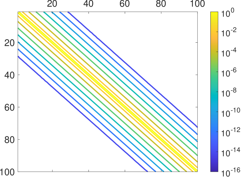
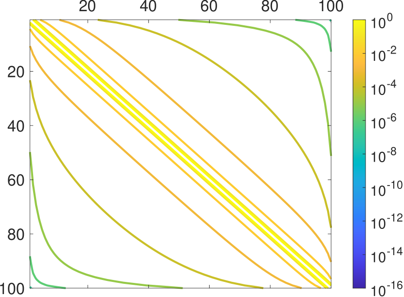
Figure 3: Plot of the matrix elements, $(\sqrt{\gamma^{\mathrm{in}}\cdot\gamma^{\mathrm{out}}})_{ij}$, for $n=100$. The horizontal and vertical axis represent $i$ and $j$, respectively. Left panel: gapped $\gamma^{\mathrm{in}}\cdot\gamma^{\mathrm{out}}$, with $\gamma^{\mathrm{in}}_{0},\gamma^{\mathrm{in}}_{1}=(3,1)$, $\gamma^{\mathrm{out}}_{0},\gamma^{\mathrm{out}}_{1}=(2,0.5)$, Right panel: gapless $\gamma^{\mathrm{in}}\cdot\gamma^{\mathrm{out}}$, with $\gamma^{\mathrm{in}}_{0},\gamma^{\mathrm{in}}_{1}=(3,1)$, $\gamma^{\mathrm{out}}_{0},\gamma^{\mathrm{out}}_{1}=(2,1)$.

The canonical jump operators $c_{k}$ of such a Lindbladian are achieved by diagonalizing $\gamma^{\mathrm{in}}$ and $\gamma^{\mathrm{out}}$, which, due to translation invariance, are given by the a discrete Fourier transform of the original $a_{j}$:

$$c_{k}=\frac{1}{\sqrt{n}}\sum_{j}e^{-\frac{2\pi i}{n}kj}a_{j},\hskip 28.45274ptk=1,\ldots,n.$$

These are in-fact non-local operators, but linear combinations of such (as anticipated by the proof of Theorem 3.2). By applying the discrete Fourier transform to 48, we see that $d^{\mathrm{in}}_{k}=\gamma^{\mathrm{in}}_{0}+2\gamma^{\mathrm{in}}_{1}\cos(\frac{2\pi k}{n})$ and similarly $d^{\mathrm{out}}_{k}=\gamma^{\mathrm{out}}_{0}+2\gamma^{\mathrm{out}}_{1}\cos(\frac{2\pi k}{n})$. Therefore, $\gamma^{\mathrm{in}},\gamma^{\mathrm{out}}$ are gapped when $\gamma^{\mathrm{in}}_{0}-2\gamma^{\mathrm{in}}_{1}=\operatorname{\Omega}\bigl{(}1\bigr{)}>0$ and $\gamma^{\mathrm{out}}_{0}-2\gamma^{\mathrm{out}}_{1}=\operatorname{\Omega}\bigl{(}1\bigr{)}>0$, respectively. We also require that $\gamma^{\mathrm{in}}_{0},\gamma^{\mathrm{out}}_{0}=\operatorname{O}\bigl{(}1\bigr{)}$ for the Lindbladian to have bounded norm. As we now show, the gaps in $\gamma^{\mathrm{in}}$ and $\gamma^{\mathrm{out}}$ stated above are responsible for the decay of the matrix elements of $\sqrt{\gamma^{\mathrm{in}}\cdot\gamma^{\mathrm{out}}}$, and therefore determine the locality of the super-Hamiltonian (47). This is due to the following lemma:

Lemma 4.4

The matrices in Eq. (48) satisfy

$$|\sqrt{\gamma^{\mathrm{in}}\cdot\gamma^{\mathrm{out}}})_{ij}|\leq 2\frac{\sqrt{\gamma^{\mathrm{in}}_{0}}}{\left(1-\frac{2\gamma^{\mathrm{in}}_{1}}{\gamma^{\mathrm{in}}_{0}}\right)^{2}}\frac{\sqrt{\gamma^{\mathrm{out}}_{0}}}{\left(1-\frac{2\gamma^{\mathrm{out}}_{1}}{\gamma^{\mathrm{out}}_{0}}\right)^{2}}\left[\left(\frac{2\gamma^{\mathrm{in}}_{1}}{\gamma^{\mathrm{in}}_{0}}\right)^{d(i,j)/2}+\left(\frac{2\gamma^{\mathrm{out}}_{1}}{\gamma^{\mathrm{out}}_{0}}\right)^{d(i,j)/2}\right]$$

where $d(i,j)\stackrel{{\scriptstyle\mathrm{def}}}{{=}}\min\{|i-j|,n-|i-j|\}$ is the metric on the circle.

As a result, provided that $\gamma^{\mathrm{in}}$ and $\gamma^{\mathrm{out}}$ are gapped, $\mathcal{H}$ given in (47) is geometrically 2-local (quadratic) with exponentially decaying interactions. The proof of Lemma 4.4 is technical and thus left to Appendix C.

We remark that the derivation in Appendix C suggests that when the gap in $\gamma^{\mathrm{in}}$ (or $\gamma^{\mathrm{out}}$) closes, that is, when $\gamma^{\mathrm{in}}_{0}=2\gamma^{\mathrm{in}}_{1}$, the super-Hamiltonian becomes long range with polynomially decaying interactions. The degree of the polynomial does not allow an area-law statement for the steady state, according to the results of Ref. [30]. See also figure 3 for an illustration of the decay in $\sqrt{\gamma^{\mathrm{in}}\cdot\gamma^{\mathrm{out}}}$.

5 Discussion and further research

In this work we have shown how a detailed-balance Lindbladian $\mathcal{L}$ can be mapped to a local, self-adjoint superoperator $\mathcal{H}$, which we call a super Hamiltonian. The mapping is via a similarity transformation, hence we are guaranteed that the Lindbladian and the super Hamiltonian share the same spectrum (up to an overall minus sign). Moreover, if $\sigma$ is the steady state of the Lindbladian, $\sqrt{\sigma}$ is the steady state of $\mathcal{H}$. By vectorizing the super Hamiltonian we get a local Hamiltonian whose ground state is $|\sigma^{1/2}\rangle\!\rangle$. As a side consequence of our mapping, we also found a necessary condition for a Lindbladian to satisfy detailed balance, which can be checked efficiently.

We observed that local expectation values in $\sigma$ map to local expectation values in the ground state $|\sigma^{1/2}\rangle\!\rangle$, and that the the mutual information in $\sigma$ is bounded by the entanglement entropy in $|\sigma^{1/2}\rangle\!\rangle$. Consequently, several well-known results about the structure of gapped ground states of local Hamiltonians can be imported to the steady state of gapped, detailed-balanced Lindbladians. In particular, we have shown how under mild conditions that can be checked efficiently, the steady state of 1D, gapped, detailed-balanced Lindbladians satisfies an area-law in mutual information, and can be well approximated by an efficient MPO. These results cover many new systems for which the results of Refs.  [21, 18] are not known to apply.

The mapping applies for Lindbladians with traceless jump operators and vanishing Hamiltonian part (a consequence of detailed balance). However, it also applies to Lindbladians with a Hamiltonian that commutes with the steady state, since it leaves the steady state invariant. An example to such a Lindbldian is the Davies generator [44] that describes thermalization. The addition of the corresponding Hamiltonian should not break primitivity [57], and we expect that in many cases it will not close the spectral gap.

Our work leaves several open questions and possible directions for future research. First, it would be interesting to see what other results/techniques can be imported from local Hamiltonians to Lindbladians using our mapping. It would also be interesting to see if this mapping can be used in numerical simulations. For example, one can apply DMRG to find the ground state of $\mathcal{H}$, and then plug it back to the Lindbladian to see if this is indeed the fixed point. Since $\mathcal{H}$ can be easily obtained from $\mathcal{L}$, this procedure can be used even if we do not know if the Lindbladian satisfies QDB.

It would also be interesting to further study the various necessary conditions that are needed to prove an area-law for steady states of local Lindbladians. In particular, it would be interesting find a concrete example of a gapped detailed-balance Lindbladian that does not obey rapid-mixing, thus separating our results from Ref. [21]. It would also be interesting to see if the conditions under which our mapping applies can be relaxed. Is there a weaker condition that still ensure a local $\mathcal{H}$?

Finally, it would also be interesting to understand if our mapping can be used in the opposite direction. Given a local Hamiltonian, one might ask if it is the vectorization of a super Hamiltonian that comes from some QDB Lindbladian. In such cases it might be possible to probe the ground state of the local Hamiltonian by simulating the time evolution of the Lindbladian on a quantum computer. This might show that the local Hamiltonian problem for this class of Hamiltonians in inside BQP. It would be interesting to characterize this class of Hamiltonians, and see if they can lead to interesting quantum algorithms.

6 Acknowledgements

We are thankful for Curt von Keyserlingk and Jens Eisert for insightful discussions. M.G. was supported by the Israel Science Foundation (ISF) and the Directorate for Defense Research and Development (DDR&D) Grant No. 3427/21, and by the US-Israel Binational Science Foundation (BSF) Grant No. 2020072. I.A. acknowledges the support of the Israel Science Foundation (ISF) under the Individual Research Grant No. 1778/17 and joint Israel-Singapore NRF-ISF Research Grant No. 3528/20.

Appendix A Proof of Lemma 3.4

In this appendix, we prove Lemma 3.4. For convenience, we first restate it here.

Lemma A.1

Let $\lambda_{\mathrm{min}}>0$ be the smallest non-zero eigenvalue of $C\cdot C^{*}$, and assume that $|C_{ab}|\leq J$ for every $a,b$. Let $|a-b|$ denote the lattice distance between the supports of $P_{a},P_{b}$. Then

$$|(C\cdot C^{*})^{1/2}_{ab}|\leq c_{1}Je^{-c_{2}|a-b|\cdot\lambda_{\mathrm{min}}/J^{2}},$$

where $c_{1},c_{2}$ are constants that depend only on the geometry of the lattice and on $k$.

• Set $A\stackrel{{\scriptstyle\mathrm{def}}}{{=}}C\cdot C^{*}$, and let $\lambda_{\mathrm{max}},\lambda_{\mathrm{min}}$ be the largest and smallest non-zero eigenvalues of $A$. Let $|a-b|$ denote the lattice distance between the support of $P_{a}$ and $P_{b}$. Recall that $C_{ab}\neq 0$ only for $P_{a},P_{b}$ that intersect a geometrically local region of $k$ sites, and therefore $C_{ab}\neq 0$ only for $|a-b|\leq k$. Similarly, for any integer $\ell>0$, $C^{\ell}_{ab}\neq 0$ only when $|a-b|\leq k\ell$, and therefore, as also $C^{*}_{ab}\neq 0$ only for $|a-b|\leq k$, we conclude that $A^{\ell}_{ab}=(C\cdot C^{*})^{\ell}_{ab}\neq 0$ only when $|a-b|\leq 2\ell k$.

  Following Ref. [58], we assume that there exists a family of polynomial approximations $\{P_{m}(z)\}$ to the function $\sqrt{z}$ (indexed by their degree) with the following properties:

  1. $|P_{m}(z)-\sqrt{z}|\leq\tau_{1}e^{-\tau_{2}m}$ for every $z\in[\lambda_{\mathrm{min}},\lambda_{\mathrm{max}}]$ for some constants $\tau_{1},\tau_{2}$ that depend on $\lambda_{\mathrm{min}},\lambda_{\mathrm{max}}$, but not on $m$.

  2. $P_{m}(0)=0$.

  We will soon find such family, but for now let us discuss its consequences.

  We first note that as the spectrum of $A$ is in $\{0\}\cup[\lambda_{\mathrm{min}},\lambda_{\mathrm{max}}]$, then for any $m$, ${\|\sqrt{A}-P_{m}(A)\|}\leq\tau_{1}e^{-\tau_{2}m}$. Consider now a pair of indices $(a,b)$, and let $m$ be the largest integer for which $2km<|a-b|$. Then by the discussion above $\big{(}P_{m}(A))_{ab}=0$, and therefore by the triangle inequality,

  $$|(\sqrt{A})_{ab}| \leq|(\sqrt{A})_{ab}-\big{(}P_{m}(A)\big{)}_{ab}|+|\big{(}P_{m}(A)\big{)}_{ab}|=|\big{(}\sqrt{A}-P_{m}(A)\big{)}_{ab}|$$

  $$\leq{\|\sqrt{A}-P_{m}(A)\|}\leq\tau_{1}e^{-m\tau_{2}}.$$

  However, as $m$ is the largest integer for which $2km<|a-b|$, then $2k(m+1)\geq|a-b|$ and therefore $m\geq|a-b|/(2k)-1$, from which we deduce

  $$|(\sqrt{A})_{ab}|\leq\tau_{1}e^{\tau_{2}}\cdot e^{-|a-b|\cdot\tau_{2}/(2k)}.$$ (49)

  Our next step is to show that the family of polynomials exists and find the dependence of $\tau_{1},\tau_{2}$ on $\lambda_{\mathrm{min}},\lambda_{\mathrm{max}}$. We will find an $m-1$ degree polynomial approximation to $1/\sqrt{z}$ in $[\lambda_{\mathrm{min}},\lambda_{\mathrm{max}}]$, and then multiply it by $z$. Following Ref. [10], we use the expansion $1/\sqrt{1+z}=\sum_{j=0}^{\infty}\left(-\frac{1}{4}\right)^{j}\binom{2j}{j}z^{j}$ in the following manner:

  $$\frac{1}{\sqrt{z}}=\frac{1}{\sqrt{\lambda_{\mathrm{max}}}}\cdot\frac{1}{\sqrt{1+(z/\lambda_{\mathrm{max}}-1)}}=\frac{1}{\sqrt{\lambda_{\mathrm{max}}}}\sum_{j=0}^{\infty}\left(-\frac{1}{4}\right)^{j}\cdot\binom{2j}{j}\cdot\left(\frac{z}{\lambda_{\mathrm{max}}}-1\right)^{j}.$$ (50)

  For $z\in[\lambda_{\mathrm{min}},\lambda_{\mathrm{max}}]$, $|z/\lambda_{\mathrm{max}}-1|<1$, and so the above series converges absolutely. Define $Q_{m}(z)$ to be the $m-1$ degree polynomial that is the sum of the terms in (50) with degree $\leq m-1$, and let $R_{m}(z)$ be the sum of all the higher order terms. Then $\frac{1}{\sqrt{z}}=Q_{m}(z)+R_{m}(z)$, and using the fact that $\binom{2j}{j}\leq 4^{j}$, we get

  $$|R_{m}(z)|\leq\frac{1}{\sqrt{\lambda_{\mathrm{max}}}}\sum_{j=m}^{\infty}|z/\lambda_{\mathrm{max}}-1|^{j}=\frac{1}{\sqrt{\lambda_{\mathrm{max}}}}\cdot\frac{|z/\lambda_{\mathrm{max}}-1|^{m}}{1-|z/\lambda_{\mathrm{max}}-1|}=\frac{\sqrt{\lambda_{\mathrm{max}}}}{z}\big{(}1-z/\lambda_{\mathrm{max}}\big{)}^{m}.$$

  Multiplying by $z$, and setting $P_{m}(z)\stackrel{{\scriptstyle\mathrm{def}}}{{=}}zQ_{m}(z)$, we find that

  $$|\sqrt{z}-P_{m}(z)|\leq\sqrt{\lambda_{\mathrm{max}}}\big{(}1-z/\lambda_{\mathrm{max}}\big{)}^{m}\leq\sqrt{\lambda_{\mathrm{max}}}e^{-mz/\lambda_{\mathrm{max}}}\leq\sqrt{\lambda_{\mathrm{max}}}e^{-m\lambda_{\mathrm{min}}/\lambda_{\mathrm{max}}}.$$

  Therefore, $\tau_{1}=\sqrt{\lambda_{\mathrm{max}}},\tau_{2}=\lambda_{\mathrm{min}}/\lambda_{\mathrm{max}}\leq 1$. Plugging to (49) yields

  $$|(C\cdot C^{*})^{1/2}_{ab}|\leq e\cdot\sqrt{\lambda_{\mathrm{max}}}\cdot e^{-|a-b|\lambda_{\mathrm{min}}/(2k\lambda_{\mathrm{max}})}.$$

  To conclude the proof, we need to show that $\lambda_{\mathrm{max}}\leq\eta J^{2}$, where $\eta$ is a constant that is a function of the lattice geometry and $k$, independent of the system size. To do that, note that $\lambda_{\mathrm{max}}={\|C\cdot C^{*}\|}\leq{\|C\|}^{2}$. By definition, $C$ is a sparse matrix, since at every row $P_{a}$ there is only a constant number of $P_{b}$ that overlap the same geometrically $k$-local region. Call this constant $\sqrt{\eta}$, and note that it only depends on $k$ and the geometry of the lattice (i.e., dimension, etc.). Therefore, assuming that $|C_{ab}|\leq J$ for all $a,b$, we deduce that for any normalized vector $v$, ${\|Cv\|}\leq J\sqrt{\eta}$, and so $\lambda_{\mathrm{max}}={\|C\|}^{2}\leq\eta J^{2}$.

   

Appendix B Classical-like Lindbladian: Technical Details

This appendix is devoted to proving bullets 3, 4 in Claim 4.1.

B.1 Proving uniqueness of the steady state (bullet 3)

We prove uniqueness of the steady state in two steps. First, we show that the steady state of the restriction of $\mathcal{L}$ to the diagonal elements is unique. Then we show that all off-diagonal elements decay due to the dissipative dynamics. We start by writing the action of the Lindbladian on a general diagonal element ${|{x}\rangle\langle{x}|}$ where $x\in\{0,1\}^{n}$:

$$\mathcal{L}({|{x}\rangle\langle{x}|})=\sum_{k,b}\gamma_{k,b}\mathcal{L}_{k,b}({|{x}\rangle\langle{x}|})=\sum_{x^{\prime}\sim x}f_{x\rightarrow x^{\prime}}{|{x^{\prime}}\rangle\langle{x^{\prime}}|}-g_{x}{|{x}\rangle\langle{x}|},$$

where the sum runs over all strings that can be achieved from $x$ by flipping one spin. The corresponding weights are give by:

$$f_{x\rightarrow x^{\prime}} =\gamma_{k,b_{k}}\cdot\begin{cases}e^{-\beta\omega_{k,b}/2},&x_{k}=1,\\ e^{\beta\omega_{k,b}/2},&x_{k}=0,\end{cases}$$

$$g_{x} =\sum_{x^{\prime}\>;\>x\rightarrow x^{\prime}}f_{x\rightarrow x^{\prime}},$$

where $b_{k}=b_{k}(x)=x_{k-1}+x_{k+1}$, and $k$ is defined by the spin that is flipped when $x\rightarrow x^{\prime}$. Note that $g_{x}$ is responsible for ensuring that $\operatorname*{Tr}\Big{(}\mathcal{L}({|{x}\rangle\langle{x}|})\Big{)}=0$.

It is known that a Lindbladian, being a generator of a CPTP semigroup, induces a (classical) continuous time Markov Process on the diagonal elements $\{{|{x}\rangle\langle{x}|}\}$ which is defined by [59]

$$P_{xy}(t)\stackrel{{\scriptstyle\mathrm{def}}}{{=}}\operatorname*{Tr}({|{x}\rangle\langle{x}|}\cdot e^{\mathcal{L}t}({|{y}\rangle\langle{y}|})).$$

To see this, Notice that $\operatorname*{Tr}\big{[}{|{x}\rangle\langle{x}|}\cdot e^{\mathcal{L}t}({|{y}\rangle\langle{y}|})\big{]}\geq 0$ due to $e^{\mathcal{L}t}$ being completely positive. One can also check the sum of each column to see that

$$\sum_{x}P_{xy}(t)=\sum_{x}\operatorname*{Tr}\big{[}{|{x}\rangle\langle{x}|}\cdot e^{\mathcal{L}t}({|{y}\rangle\langle{y}|})\big{]}=\operatorname*{Tr}\big{[}e^{\mathcal{L}t}({|{y}\rangle\langle{y}|})\big{]}=1,$$

due to $e^{\mathcal{L}t}$ being trace preserving. To deduce the uniqueness of a stationary distribution of $P_{xy}$, we use the Perron-Frobenious Theorem and the connectivity of the Markov chain. Specifically, we show that $P_{xy}(t)>0$ for any $x,y,t$, and uniqueness will follow as a consequence from Perron-Frobenious (see Theorem 1.1 in Ref. [39]).

Claim B.1

$P_{xy}(t)=\operatorname*{Tr}\big{[}{|{x}\rangle\langle{x}|}e^{\mathcal{L}t}({|{y}\rangle\langle{y}|})\big{]}>0$ for any $t>0$.

• Let $G=(V,E)$ be a graph where $V=\{0,1\}^{n}$ is the set of bit-strings and $(x,x^{\prime})\in E$ if and only if they have Hamming distance $d_{H}(x,x^{\prime})=1$ ($x^{\prime}$ is obtained from $x$ by flipping one bit). Notice that this is also the connectivity graph of $\mathcal{L}$ with self edges omitted. For $x,y\in V$, define $\ell=(\ell_{0},\ldots,\ell_{|\ell|+1})$ to be the shortest path in $G$ from $x$ to $y$ (i.e. $d_{H}(x,y)=|\ell|$). Take $c>0$ such that $c>g_{z}$ for any $z\in V$. As a result, $(\mathcal{L}t+c\mathbbm{1})_{xy}\geq 0$ for any $x,y$, and in particular $(\mathcal{L}+c\mathbbm{1})_{xy}>0$ if $(x,y)\in E$. Let us expand $e^{\mathcal{L}t}$

  $$e^{\mathcal{L}t}=e^{-c}e^{\mathcal{L}t+c\mathbbm{1}}=e^{-c}\sum_{k=0}^{\infty}\frac{1}{k!}(\mathcal{L}t+c\mathbbm{1})^{k}.$$ (51)

  Notice that $\left((\mathcal{L}t+c\mathbbm{1})^{k}\right)_{xy}\neq 0$ if and only if $d_{H}(x,y)\leq k$, therefore $P_{xy}$ receives its first non-zero contributions from the $k=|\ell|$th order in the expansion. Moreover, this first contribution is positive, since

  $${\langle{x|(\mathcal{L}t+c\mathbbm{1})^{k}|y}\rangle} =\sum_{r_{1},\ldots,r_{k-1}}{\langle{x|\mathcal{L}t+c\mathbbm{1}|r_{1}}\rangle}{\langle{r_{1}|\mathcal{L}t+c\mathbbm{1}|r_{2}}\rangle}\ldots{\langle{r_{k-1}|\mathcal{L}t+c\mathbbm{1}|y}\rangle}$$

  $$={\langle{x|\mathcal{L}t+c\mathbbm{1}|\ell_{1}}\rangle}{\langle{\ell_{1}|\mathcal{L}t+c\mathbbm{1}|\ell_{2}}\rangle}\ldots{\langle{\ell_{k-1}|\mathcal{L}t+c\mathbbm{1}|y}\rangle}$$

  $$+\sum_{\{r_{1},\ldots,r_{k-1}\}\neq\ell}{\langle{x|\mathcal{L}t+c\mathbbm{1}|r_{1}}\rangle}{\langle{r_{1}|\mathcal{L}t+c\mathbbm{1}|r_{2}}\rangle}\ldots{\langle{r_{k-1}|\mathcal{L}t+c\mathbbm{1}|y}\rangle}>0,$$

  where we abuse of notation by writing ${\langle{x|\mathcal{T}|y}\rangle}$ instead of $\operatorname*{Tr}\big{[}{|{x}\rangle\langle{x}|}\cdot\mathcal{T}({|{y}\rangle\langle{y}|})\big{]}$, exploiting the fact that the action of $\mathcal{T}=\mathcal{L}t+c\mathbbm{1}$ is closed on the diagonal elements ${|{x}\rangle\langle{x}|}$. Notice that the first term after the equality sign is greater than zero using the path $\ell$ and graph connectivity of the semigroup, and the rest of the sum is greater than or equal to zero, hence the whole term is greater than zero. The higher $k$ terms are greater or equal to zero (since all matrix elements are), thus we conclude the claim.  

The only thing left to show now is that the off-diagonal elements decay. Let us write the action of the Lindbladian on the off diagonal terms explicitly:

$$\mathcal{L}({|{x}\rangle\langle{y}|})=\sum_{x^{\prime},y^{\prime}}f_{xy\rightarrow x^{\prime}y^{\prime}}{|{x^{\prime}}\rangle\langle{y^{\prime}}|}-\left(\frac{1}{2}g_{x}+\frac{1}{2}g_{y}\right){|{x}\rangle\langle{y}|},$$

where $f_{xy\rightarrow x^{\prime}y^{\prime}}$ is non-zero only if there are $k\in\{1,\ldots,n\}$ and $b\in\{0,1,2\}$ such that $L_{k,b}{|{x}\rangle\langle{y}|}L_{k,b}^{\dagger}\neq 0$ or $L_{k,b}^{\dagger}{|{x}\rangle\langle{y}|}L_{k,b}\neq 0$ (that is, if $x_{k}=y_{k}$, $x_{k-1}+x_{k+1}=y_{k-1}+y_{k+1}$), and then it would give $f_{xy\rightarrow x^{\prime}y^{\prime}}=f_{x\rightarrow x^{\prime}}=f_{y\rightarrow y^{\prime}}$. The observation is that

$$\sum_{(x^{\prime},y^{\prime})}f_{xy\rightarrow x^{\prime}y^{\prime}}<\frac{1}{2}g_{x}+\frac{1}{2}g_{y},$$

namely, looking at the representing matrix $\mathcal{L}|_{\{{|{m}\rangle\langle{n}|}\}_{m\neq n}}$, the sum of the off-diagonal elements in each column is strictly smaller than the absolute value of the element on the diagonal. We claim that the eigenvalues of such matrix must be strictly negative.

Claim B.2

Let $A_{ij}$ be a matrix with non-negative off diagonal elements and strictly negative diagonal elements, such that $\sum_{j\;;\;j\neq i}A_{ij}<-A_{ii}$ for any $i$. Then $\mathrm{Spec}(A)\subset(-\infty,0)$.

• Consider the exponentiation of $A$. This is a semi-stochastic matrix (its matrix-elements are non-negative), since

  $$e^{A}=e^{-c}e^{A+c\mathbbm{1}}=e^{-c}\sum_{k=0}^{\infty}\frac{1}{k!}\left(A+c\mathbbm{1}\right)^{k}$$

  where $c>0$ is chosen such that $A_{ii}+c>0$ for each $i$. Therefore, $(A+c\mathbbm{1})_{i,j}$, and correspondingly $(e^{A})_{ij}$, are greater or equal to zero for any $i,j$. Using the Perron-Frobenious Theorem, $e^{A}$ has a maximal eigenvalue $r>0$ with an eigenvector $v$ in which $v_{i}\geq 0$ for any $i$. We deduce that $v$ is also an eigenvector of $A$ with largest eigenvalue, due to the monotonicity of the exponent:

  $$\sum_{j}A_{ij}v_{j}=\lambda v_{i}\hskip 28.45274pt\forall i.$$ (52)

  We finally show that $\lambda$ is negative due to the assumption in the claim, and the remaining spectrum will be negative as well (since it must be below $\lambda$). Indeed, let $i_{0}=\arg\max\{v_{i}\}$, and take

  $$\lambda v_{i_{0}}=\sum_{j}A_{i_{0}j}v_{j}=A_{i_{0}i_{0}}v_{i_{0}}+\sum_{j\neq i_{0}}A_{i_{0}j}v_{j}\leq A_{i_{0}i_{0}}v_{i_{0}}+v_{i_{0}}\sum_{j\neq i_{0}}A_{i_{0}j}<0,$$

  where in the last inequality we used $\sum_{j\neq i}A_{ij}<-A_{ii}$.  

B.2 Proving that $\mathcal{L}$ is gapped (bullet 4)

To show a gap in the system, we import the finite-size criteria for frustration-free Hamiltonians, originally introduced by Knabe [33] and used, for example, in Refs.  [34, 51]. First we introduce the method for generic systems defined on finite dimensional Hilbert spaces, and then use it to show a gap for the system under consideration. We change our notation correspondingly, e.g., we first discuss projectors on a generic Hilbert space and denote them by $P_{e}$, and in the next paragraph we refer to projectors on operators space (super-projectors) which we denote by $\mathcal{P}_{e}$.

Claim B.3 (Finite size criteria)

Let $G=(V,E)$ be a regular graph of degree $\delta$. Assign a local Hilbert-space of dimension $d$ to each vertex. Let $H$ be a nearest-neighbors frustration free Hamiltonian defined on the joint Hilbert space of the vertices of the form:

$$H=\sum_{e\in E}P_{e},$$ (53)

where each $P_{e}$ is a projector defined on the bond $e$. We define the local gap to be $\gamma_{loc}\stackrel{{\scriptstyle\mathrm{def}}}{{=}}\min_{e\cap e^{\prime}\neq\emptyset}\left(\operatorname{gap}\left[P_{e}+P_{e^{\prime}}\right]\right)$. Then

$$\operatorname{gap}{(H)}\geq 2(\delta-1)\left(\gamma_{loc}-\left(1-1/2(\delta-1)\right)\right).$$ (54)

• Note that due to frustration-freeness and spectral decomposition, an inequality of the form

  $$H^{2}\geq c\cdot H$$ (55)

  immediately implies that $\operatorname{gap}(H)\geq c$. This is the principle that lies at heart of the method. To achieve a bound of the form (55), Knabe used the Hamiltonian’s local structure and the local spectral gap, as explained in the following. We start by squaring $H$ and rearranging the double sum:

  $$H^{2}=\left(\sum_{e}P_{e}\right)^{2}=\sum_{e}P_{e}^{2}+\sum_{e\cap e^{\prime}\neq\emptyset}(P_{e}\cdot P_{e^{\prime}}+P_{e^{\prime}}\cdot P_{e})+2\sum_{e\cap e^{\prime}=\emptyset}P_{e}\cdot P_{e^{\prime}}.$$ (56)

  Since we are looking for an inequality of the form $H^{2}\geq cH$, we can ignore the rightmost term in (56), as it is positive semi-definite, being a sum of products of non-overlapping projectors. Using $P_{e}^{2}=P_{e}$, one should notice that the first term in Eq. (56) reduces to $H$ itself. Hence we obtained $H^{2}\geq H+Q$, where $Q\stackrel{{\scriptstyle\mathrm{def}}}{{=}}\sum_{e\cap e^{\prime}\neq\emptyset}P_{e}\cdot P_{e^{\prime}}+P_{e^{\prime}}\cdot P_{e}$. To achieve the desired bound, we write down a lower bound for $Q$ using $H$. To do so, let us consider

  $$\sum_{e\cap e^{\prime}\neq\emptyset}\left(P_{e}+P_{e^{\prime}}\right)^{2}.$$

  Expanding the square, we see that the expression equals

  $$\sum_{e\cap e^{\prime}\neq\emptyset}\left(P_{e}+P_{e^{\prime}}+P_{e}P_{e^{\prime}}+P_{e^{\prime}}P_{e}\right)=2(\delta-1)\cdot H+Q,$$

  where the $2(\delta-1)$ factor stems from the fact that for a simple regular graph, each edge intersects $2(\delta-1)$ distinct edges ($\delta-1$ on each vertex). On the other hand, due to frustration freeness, we have $\left(P_{e}+P_{e^{\prime}}\right)^{2}\geq\operatorname{gap}\left[P_{e}+P_{e^{\prime}}\right]\left(P_{e}+P_{e^{\prime}}\right)$, and obtain

  $$2(\delta-1)\cdot H+Q\geq 2(\delta-1)\gamma_{loc}\cdot H.$$

  Plugging this into Eq. (56) gives

  $$H^{2}\geq H+Q\geq 2(\delta-1)\cdot H\left(\gamma_{loc}-\left(1-\frac{1}{2(\delta-1)}\right)\right).$$ (57)

  Using inequality (55) ($H^{2}\geq c\cdot H$) for $c=2(\delta-1)\left(\gamma_{loc}-\left(1-\frac{1}{2(\delta-1)}\right)\right)$, we see that

  $$\operatorname{gap}(H)\geq 2(\delta-1)\left(\gamma_{loc}-\left(1-\frac{1}{2(\delta-1)}\right)\right),$$

  meaning that if $\gamma_{loc}$ is greater than $1-\frac{1}{2(\delta-1)}$, a global gap in $H$ confirmed.  

We remark that the method can be generalized to larger sub-regions and to open boundary conditions [33, 60].

Application to $\mathcal{H}$

Now we apply the method to the system under consideration to show a global gap in $\mathcal{L}$, thus completing bullet 4 of Claim 4.1. First, we reduce the super-Hamiltonian to the sum-of-local-projectors Hamiltonian presented in Eq. (53) (up to a multiplicative factor). Then, we numerically verify the statement that $\gamma_{loc}>1-\frac{1}{2(\delta-1)}=\frac{1}{2}$ for the 1D ring, which will assure the global gap by Eq. (57).

Recall the parent Hamiltonian, $\mathcal{H}=\sum_{k,b}\gamma_{k,b}\mathcal{H}_{k,b}$, where $\mathcal{H}_{k,b}=-\Gamma_{s}^{-1/2}\circ\mathcal{L}_{k,b}\circ\Gamma_{s}^{1/2}$ and $\gamma_{k,b}\geq\alpha>0$. Also recall that $\mathcal{H}$ is frustration-free, where $\mathcal{H}_{k,b}\geq 0$ has a ground state $\sqrt{\sigma}$ with energy $0$. Then $\mathcal{H}$ satisfies

$$\mathcal{H} \geq\alpha\sum_{k,b}\mathcal{H}_{k,b}=\alpha\sum_{k}\mathcal{H}_{k},$$

$$\mathrm{where} \hskip 28.45274pt\mathcal{H}_{k}\stackrel{{\scriptstyle\mathrm{def}}}{{=}}\sum_{b=0,1,2}\mathcal{H}_{k,b}.$$

Let $\mathcal{P}_{k}$ denote the local projector onto the positive spectrum of $\mathcal{H}_{k}$ such that $\mathcal{H}_{k}\geq g_{k}\mathcal{P}_{k}$ where $g_{k}\stackrel{{\scriptstyle\mathrm{def}}}{{=}}\operatorname{gap}(\mathcal{H}_{k})$. By simply calculating the spectrum of $\mathcal{H}_{k}$ we see that $g_{k}=\min_{b\in\{0,1,2\}}\{e^{\beta\omega_{k,b}}\}=e^{-\beta(\epsilon_{k}-\mu+2u)}$, which is of order $1$ provided that $\epsilon_{k}-\mu,u=\operatorname{O}\bigl{(}1\bigr{)}$. We thus conclude that

$$\mathcal{H}\geq\alpha g_{\min}\sum_{k}\mathcal{P}_{k},$$

where we defined $g_{\min}\stackrel{{\scriptstyle\mathrm{def}}}{{=}}\min_{k}g_{k}$. Moreover, since both sides have a common ground space which is spannded by $\sqrt{\sigma}$ with ground energy $0$, using Claim B.3 we have

$$\operatorname{gap}(\mathcal{H})\geq\alpha g_{\min}\operatorname{gap}\left(\sum_{k}\mathcal{P}_{k}\right)\geq 2\alpha g_{\min}(\gamma_{loc}-1/2),$$

where $\gamma_{loc}=\min_{k}\operatorname{gap}(\mathcal{P}_{k}+\mathcal{P}_{k+1})$. To show a gap in $\mathcal{H}$, we assure that $\operatorname{gap}(\mathcal{P}_{k}+\mathcal{P}_{k+1})>1/2$. Instead of giving a tedious derivation of the local gap, we numerically verify it in the following table for $\mu=0$ and different choices of $\{\epsilon_{k}\}$ and $u$.

Local Gap $\gamma_{loc}$
Model	u=-1	u=0.5	u=2
Random $\{\epsilon_{k}\}$	0.756	0.887	0.678
Const $\epsilon_{k}=1$	0.769	0.913	0.778
Const $\epsilon_{k}=0.5$	0.755	0.891	0.698
$\epsilon_{1}=1$, $\epsilon_{2}=10$	0.993	0.998	0.997

We remark that the derivation of the finite size criteria considers 2-local interaction (graph interactions), and the model under consideration here is 3-local. However, the derivation and results are still valid. This is due to terms that overlap on a single qubit (e.g. $\mathcal{H}_{k}$ and $\mathcal{H}_{k+2}$) commute with each other, as they act trivially on their shared qubits. Therefore, when squaring $\mathcal{H}$ in Eq. (56), their product can be absorbed in the positive ”leftover” (the last term in (56)).

Appendix C Quadratic fermionic Lindbladians: Technical Details

This appendix is devoted to proving Lemma 4.4, which demonstrates the exponential decay in the coefficients of the super-Hamiltonian with respect to the distance between the real space fermionic operators.

First, recall the settings of the lemma. To relate the model to the subject of our work, which discusses local Lindbladians that satisfy quantum detailed-balance, we focus on commuting $\gamma^{\mathrm{in}},\gamma^{\mathrm{out}}$ that connect nearest neighbours (i.e. tridiagonal matrices). For simplicity, we consider translation invariant systems, such that

$$\gamma^{\mathrm{in}}=\begin{pmatrix}\gamma^{\mathrm{in}}_{0}&\gamma^{\mathrm{in}}_{1}&0&&\ldots&0&\gamma^{\mathrm{in}}_{1}\\ \gamma^{\mathrm{in}}_{1}&\gamma^{\mathrm{in}}_{0}&\gamma^{\mathrm{in}}_{1}&&&&0\\ 0&\gamma^{\mathrm{in}}_{1}&\gamma^{\mathrm{in}}_{0}&\\ \vdots&&&\ddots&&&\vdots\\ &&&&\gamma^{\mathrm{in}}_{0}&\gamma^{\mathrm{in}}_{1}&0\\ 0&&&&\gamma^{\mathrm{in}}_{1}&\gamma^{\mathrm{in}}_{0}&\gamma^{\mathrm{in}}_{1}\\ \gamma^{\mathrm{in}}_{1}&0&&\ldots&0&\gamma^{\mathrm{in}}_{1}&\gamma^{\mathrm{in}}_{0}\end{pmatrix},\quad\gamma^{\mathrm{out}}=\begin{pmatrix}\gamma^{\mathrm{out}}_{0}&\gamma^{\mathrm{out}}_{1}&0&&\ldots&0&\gamma^{\mathrm{out}}_{1}\\ \gamma^{\mathrm{out}}_{1}&\gamma^{\mathrm{out}}_{0}&\gamma^{\mathrm{out}}_{1}&&&&0\\ 0&\gamma^{\mathrm{out}}_{1}&\gamma^{\mathrm{out}}_{0}&\\ \vdots&&&\ddots&&&\vdots\\ &&&&\gamma^{\mathrm{out}}_{0}&\gamma^{\mathrm{out}}_{1}&0\\ 0&&&&\gamma^{\mathrm{out}}_{1}&\gamma^{\mathrm{out}}_{0}&\gamma^{\mathrm{out}}_{1}\\ \gamma^{\mathrm{out}}_{1}&0&&\ldots&0&\gamma^{\mathrm{out}}_{1}&\gamma^{\mathrm{out}}_{0}\end{pmatrix}.$$

The canonical jump operators are given by a discrete Fourier transform of the original $a_{k}$:

$$c_{k}=\frac{1}{\sqrt{n}}\sum_{j}e^{-\frac{2\pi i}{n}kj}a_{j},\quad k=1\cdots n.$$

These are non-local operators, but a linear combination of such.

To prove the lemma, we want to show that the matrix $\sqrt{\gamma^{\mathrm{in}}}\cdot\sqrt{\gamma^{\mathrm{out}}}$ has elements that decay exponentially with the distance from the main diagonal. First, we show that $\sqrt{\gamma^{\mathrm{in}}}$ and $\sqrt{\gamma^{\mathrm{out}}}$ individually satisfy

$$(\sqrt{\gamma^{\mathrm{in}}})_{ij}=O\left(\frac{\sqrt{\gamma^{\mathrm{in}}_{0}}}{1-\frac{2\gamma^{\mathrm{in}}_{1}}{\gamma^{\mathrm{in}}_{0}}}\left(\frac{2\gamma^{\mathrm{in}}_{1}}{\gamma^{\mathrm{in}}_{0}}\right)^{d(i,j)}\right),\hskip 28.45274pt(\sqrt{\gamma^{\mathrm{out}}})_{ij}=O\left(\frac{\sqrt{\gamma^{\mathrm{out}}_{0}}}{1-\frac{2\gamma^{\mathrm{out}}_{1}}{\gamma^{\mathrm{out}}_{0}}}\left(\frac{2\gamma^{\mathrm{out}}_{1}}{\gamma^{\mathrm{out}}_{0}}\right)^{d(i,j)}\right).$$

Then, we use this to establish an upper-bound on $\sqrt{\gamma^{\mathrm{in}}\cdot\gamma^{\mathrm{out}}}_{ij}$.

To show a decay in $\gamma^{\mathrm{in}}$ (the treatment of $\gamma^{\mathrm{out}}$ is identical), we notice that

$$\gamma^{\mathrm{in}}=\begin{pmatrix}\gamma^{\mathrm{in}}_{0}&&&&\\ &\gamma^{\mathrm{in}}_{0}&&&\\ &&\ddots&&\\ &&&&\gamma^{\mathrm{in}}_{0}&\\ &&&&&\gamma^{\mathrm{in}}_{0}\end{pmatrix}+\begin{pmatrix}0&\gamma^{\mathrm{in}}_{1}&&&\gamma^{\mathrm{in}}_{1}\\ \gamma^{\mathrm{in}}_{1}&0&\gamma^{\mathrm{in}}_{1}&\\ &&\ddots&&\\ &&\gamma^{\mathrm{in}}_{1}&0&\gamma^{\mathrm{in}}_{1}\\ \gamma^{\mathrm{in}}_{1}&&&\gamma^{\mathrm{in}}_{1}&0\end{pmatrix}\stackrel{{\scriptstyle\mathrm{def}}}{{=}}\gamma^{\mathrm{in}}_{0}\mathbbm{1}+2\gamma^{\mathrm{in}}_{1}W.$$

A key observation is that $W$ is the (symmetric) random walk matrix $W_{ij}=\frac{1}{2}\delta_{j,i\pm 1}$. Plugging the Taylor expansion $\sqrt{1+x}=\sum_{k\geq 0}\alpha_{k}x^{k}$ produces

$$\sqrt{\gamma^{\mathrm{in}}}=\sqrt{\gamma^{\mathrm{in}}_{0}\mathbbm{1}+2\gamma^{\mathrm{in}}_{1}W}=\sqrt{\gamma^{\mathrm{in}}_{0}}\sqrt{\mathbbm{1}+\frac{2\gamma^{\mathrm{in}}_{1}}{\gamma^{\mathrm{in}}_{0}}W}=\sqrt{\gamma^{\mathrm{in}}_{0}}\sum_{k\geq 0}\alpha_{k}\left(\frac{2\gamma^{\mathrm{in}}_{1}}{\gamma^{\mathrm{in}}_{0}}\right)^{k}W^{k}.$$

Note that $(W^{k})_{ij}$ is the transition probability for $i\rightarrow j$ after $k$ steps of the walk, which is less than one and non-zero only when $k\geq\min\{|i-j|,n-|i-j|\}$; Assume without loss of generality that the minimum is attained at $|i-j|$. Moreover, the sequence $\{\alpha_{k}\}$ is smaller than one in absolute value (polynomially decaying to be precise). Then the matrix entry $(\sqrt{\gamma^{\mathrm{in}}})_{i,j}$ satisfies

$$(\sqrt{\gamma^{\mathrm{in}}})_{i,j}=\sqrt{\gamma^{\mathrm{in}}_{0}}\sum_{k\geq 0}\alpha_{k}\left(\frac{2\gamma^{\mathrm{in}}_{1}}{\gamma^{\mathrm{in}}_{0}}\right)^{n}(W^{k})_{ij}\leq\sqrt{\gamma^{\mathrm{in}}_{0}}\sum_{k\geq|i-j|}\left(\frac{2\gamma^{\mathrm{in}}_{1}}{\gamma^{\mathrm{in}}_{0}}\right)^{k}=\left(\frac{2\gamma^{\mathrm{in}}_{1}}{\gamma^{\mathrm{in}}_{0}}\right)^{|i-j|}\left(\frac{\sqrt{\gamma^{\mathrm{in}}_{0}}}{1-\frac{2\gamma^{\mathrm{in}}_{1}}{\gamma^{\mathrm{in}}_{0}}}\right).$$ (58)

This shows that $(\sqrt{\gamma^{\mathrm{in}}})_{ij}=\operatorname{O}\bigl{(}e^{-|i-j|}\bigr{)}$ provided that $\gamma^{\mathrm{in}}$ is gapped and ${\|\gamma^{\mathrm{in}}\|}=\operatorname{O}\bigl{(}1\bigr{)}$. The analogous argument for $\gamma^{\mathrm{out}}$ is straightforward. Note that for $\gamma^{\mathrm{in}}_{0}=2\gamma^{\mathrm{in}}_{1}$, the gap in $\gamma^{\mathrm{in}}$ closes, and a polynomial decay in $\sqrt{\gamma^{\mathrm{in}}}_{ij}$ appears instead (see Figure 3). This is because for large $k$’s, the probability for the random walk yields $(W^{k})_{ij}=\frac{1}{2^{k+1}}{\binom{k}{\frac{|i-j|+k}{2}}}=\operatorname{O}\bigl{(}k^{-1/2}\bigr{)}$ (see page 291 in Ref. [61]), and also we get that $\alpha_{k}=\operatorname{O}\bigl{(}\frac{1}{k}\bigr{)}$.

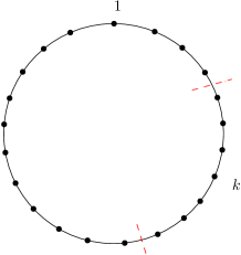
Figure 4: The neighborhoods for the partial sums in the calculation for $B_{1k}$.

It is now left to show that the product $B\stackrel{{\scriptstyle\mathrm{def}}}{{=}}\sqrt{\gamma^{\mathrm{in}}\cdot\gamma^{\mathrm{out}}}$ has exponentially decaying matrix elements as well. We show this for first row elements $B_{1k}$ for convenience, as it automatically generalized to any $B_{ij}$ due to translation invariance. Let us write down $B_{1k}$, explicitly and use the former bounds for $\sqrt{\gamma^{\mathrm{in}}}$ and $\sqrt{\gamma^{\mathrm{out}}}$. Suppose that $k\leq n/2$ as before; then

$$|B_{1k}| \leq\sum_{m}|\sqrt{\gamma^{\mathrm{in}}}_{1m}\sqrt{\gamma^{\mathrm{out}}}_{mk}|$$

$$\leq\sum_{m}\frac{\sqrt{\gamma^{\mathrm{in}}_{0}}}{1-\frac{2\gamma^{\mathrm{in}}_{1}}{\gamma^{\mathrm{in}}_{0}}}\frac{\sqrt{\gamma^{\mathrm{out}}_{0}}}{1-\frac{2\gamma^{\mathrm{out}}_{1}}{\gamma^{\mathrm{out}}_{0}}}\left(\frac{2\gamma^{\mathrm{in}}_{1}}{\gamma^{\mathrm{in}}_{0}}\right)^{d(m,1)}\left(\frac{2\gamma^{\mathrm{out}}_{1}}{\gamma^{\mathrm{out}}_{0}}\right)^{d(k,m)}$$

$$=\frac{\sqrt{\gamma^{\mathrm{in}}_{0}}}{1-\frac{2\gamma^{\mathrm{in}}_{1}}{\gamma^{\mathrm{in}}_{0}}}\frac{\sqrt{\gamma^{\mathrm{out}}_{0}}}{1-\frac{2\gamma^{\mathrm{out}}_{1}}{\gamma^{\mathrm{out}}_{0}}}\left[\sum_{m=k/2+1}^{k+k/2}\left(\frac{2\gamma^{\mathrm{in}}_{1}}{\gamma^{\mathrm{in}}_{0}}\right)^{d(m,1)}\left(\frac{2\gamma^{\mathrm{out}}_{1}}{\gamma^{\mathrm{out}}_{0}}\right)^{d(k,m)}+\sum_{m=3k/2+1}^{k/2}\left(\frac{2\gamma^{\mathrm{in}}_{1}}{\gamma^{\mathrm{in}}_{0}}\right)^{d(m,1)}\left(\frac{2\gamma^{\mathrm{out}}_{1}}{\gamma^{\mathrm{out}}_{0}}\right)^{d(k,m)}\right],$$

where the last sum is performed periodically, i.e. $m=3k/2+1,3k/2+2,\ldots,n-1,n,1,2,\ldots,k/2$. All we did is to separate the sum to a $k/2$ length neighbourhood of the $k$th site and the complement (see Figure 4). At the first sum, the decay is dominated by $\left(\frac{2\gamma^{\mathrm{in}}_{1}}{\gamma^{\mathrm{in}}_{0}}\right)^{d(m,1)}=\left(\frac{2\gamma^{\mathrm{in}}_{1}}{\gamma^{\mathrm{in}}_{0}}\right)^{m-1}\leq\left(\frac{2\gamma^{\mathrm{in}}_{1}}{\gamma^{\mathrm{in}}_{0}}\right)^{k/2}$, and at the second sum the $\left(\frac{2\gamma^{\mathrm{out}}_{1}}{\gamma^{\mathrm{out}}_{0}}\right)^{d(k,m)}\leq\left(\frac{2\gamma^{\mathrm{out}}_{1}}{\gamma^{\mathrm{out}}_{0}}\right)^{k/2}$ term dominates. Therefore we write

$$|B_{1k}|\leq\frac{\sqrt{\gamma^{\mathrm{in}}_{0}}}{1-\frac{2\gamma^{\mathrm{in}}_{1}}{\gamma^{\mathrm{in}}_{0}}}\frac{\sqrt{\gamma^{\mathrm{out}}_{0}}}{1-\frac{2\gamma^{\mathrm{out}}_{1}}{\gamma^{\mathrm{out}}_{0}}}\left[\sum_{m=k/2+1}^{k+k/2}\left(\frac{2\gamma^{\mathrm{in}}_{1}}{\gamma^{\mathrm{in}}_{0}}\right)^{m-1}+\sum_{m=3k/2+1}^{k/2}\left(\frac{2\gamma^{\mathrm{out}}_{1}}{\gamma^{\mathrm{out}}_{0}}\right)^{d(k,m)}\right],$$

where we used the fact that both $\frac{2\gamma^{\mathrm{in}}_{1}}{\gamma^{\mathrm{in}}_{0}}$ and $\frac{2\gamma^{\mathrm{out}}_{1}}{\gamma^{\mathrm{out}}_{0}}$ are smaller than $1$. Since both sums are geometric, they can be bounded to achieve the desired bound

$$|B_{1k}|\leq 2\frac{\sqrt{\gamma^{\mathrm{in}}_{0}}}{\left(1-\frac{2\gamma^{\mathrm{in}}_{1}}{\gamma^{\mathrm{in}}_{0}}\right)^{2}}\frac{\sqrt{\gamma^{\mathrm{out}}_{0}}}{\left(1-\frac{2\gamma^{\mathrm{out}}_{1}}{\gamma^{\mathrm{out}}_{0}}\right)^{2}}\left[\left(\frac{2\gamma^{\mathrm{in}}_{1}}{\gamma^{\mathrm{in}}_{0}}\right)^{k/2}+\left(\frac{2\gamma^{\mathrm{out}}_{1}}{\gamma^{\mathrm{out}}_{0}}\right)^{k/2}\right].$$

References

• [1] A. Y. Kitaev, A. Shen, M. N. Vyalyi, and M. N. Vyalyi, Classical and quantum computation. No. 47 in Graduate Studies in Mathematics, American Mathematical Soc., 2002.
• [2] J. Kempe, A. Kitaev, and O. Regev, “The Complexity of the Local Hamiltonian Problem,” SIAM Journal on Computing, vol. 35, no. 5, pp. 1070–1097, 2006.
• [3] J. Eisert, M. Cramer, and M. B. Plenio, “Area laws for the entanglement entropy - a review,” Reviews of Modern Physics, vol. 82, pp. 277–306, 2010.
• [4] M. B. Hastings, “An area law for one-dimensional quantum systems,” Journal of Statistical Mechanics: Theory and Experiment, pp. 8024–8024, Aug 2007.
• [5] L. Masanes, “Area law for the entropy of low-energy states,” Phys. Rev. A, vol. 80, p. 052104, Nov 2009.
• [6] N. de Beaudrap, T. J. Osborne, and J. Eisert, “Ground states of unfrustrated spin Hamiltonians satisfy an area law,” New Journal of Physics, vol. 12, p. 095007, sep 2010.
• [7] S. Michalakis, “Stability of the area law for the entropy of entanglement,” arXiv preprint arXiv:1206.6900, 2012.
• [8] J. Cho, “Sufficient Condition for Entanglement Area Laws in Thermodynamically Gapped Spin Systems,” Phys. Rev. Lett., vol. 113, p. 197204, Nov 2014.
• [9] F. G. S. L. Brandão and M. Cramer, “Entanglement area law from specific heat capacity,” Phys. Rev. B, vol. 92, p. 115134, Sep 2015.
• [10] A. Anshu, I. Arad, and D. Gosset, “Entanglement Subvolume Law for 2D Frustration-Free Spin Systems,” Communications in Mathematical Physics, vol. 393, Jul 2022.
• [11] A. Anshu, I. Arad, and D. Gosset, “An area law for 2D frustration-free spin systems,” arXiv preprint arXiv:2103.02492, 2021.
• [12] G. Agarwal, “Open quantum markovian systems and the microreversibility,” Zeitschrift für Physik A Hadrons and nuclei, vol. 258, no. 5, pp. 409–422, 1973.
• [13] R. Alicki, “On the detailed balance condition for non-hamiltonian systems,” Reports on Mathematical Physics, vol. 10, no. 2, pp. 249–258, 1976.
• [14] F. Fagnola and V. Umanità, “Generators of detailed balance quantum markov semigroups,” Infinite Dimensional Analysis, Quantum Probability and Related Topics, vol. 10, no. 03, pp. 335–363, 2007.
• [15] K. Temme, M. J. Kastoryano, M. B. Ruskai, M. M. Wolf, and F. Verstraete, “The $\chi^{2}$-divergence and mixing times of quantum markov processes,” Journal of Mathematical Physics, vol. 51, no. 12, p. 122201, 2010.
• [16] E. A. Carlen and J. Maas, “Gradient flow and entropy inequalities for quantum markov semigroups with detailed balance,” Journal of Functional Analysis, vol. 273, no. 5, pp. 1810–1869, 2017.
• [17] R. Alicki, M. Fannes, and M. Horodecki, “On thermalization in kitaev’s 2d model,” Journal of Physics A: Mathematical and Theoretical, vol. 42, no. 6, p. 065303, 2009.
• [18] M. J. Kastoryano and J. Eisert, “Rapid mixing implies exponential decay of correlations,” Journal of Mathematical Physics, vol. 54, no. 10, p. 102201, 2013.
• [19] M. J. Kastoryano and F. G. Brandao, “Quantum gibbs samplers: The commuting case,” Communications in Mathematical Physics, vol. 344, no. 3, pp. 915–957, 2016.
• [20] P. Wocjan and K. Temme, “Szegedy walk unitaries for quantum maps,” arXiv preprint arXiv:2107.07365, 2021.
• [21] F. G. S. L. Brandão, T. S. Cubitt, A. Lucia, S. Michalakis, and D. Perez-Garcia, “Area law for fixed points of rapidly mixing dissipative quantum systems,” Journal of Mathematical Physics, vol. 56, no. 10, p. 102202, 2015.
• [22] R. Trivedi and J. I. Cirac, “Simulatability of locally-interacting open quantum spin systems,” arXiv preprint arXiv:2110.10638, 2021.
• [23] R. Mahajan, C. D. Freeman, S. Mumford, N. Tubman, and B. Swingle, “Entanglement structure of non-equilibrium steady states,” arXiv preprint arXiv:1608.05074, 2016.
• [24] M. J. Kastoryano and K. Temme, “Quantum logarithmic sobolev inequalities and rapid mixing,” Journal of Mathematical Physics, vol. 54, no. 5, p. 052202, 2013.
• [25] D. Poulin, “Lieb-Robinson Bound and Locality for General Markovian Quantum Dynamics,” Phys. Rev. Lett., vol. 104, p. 190401, May 2010.
• [26] B. Nachtergaele, A. Vershynina, and V. A. Zagrebnov, Lieb-Robinson bounds and existence of the thermodynamic limit for a class of irreversible quantum dynamics., vol. 552 of Entropy and the quantum II. American Mathematical Soc., 2011.
• [27] T. Barthel and M. Kliesch, “Quasilocality and Efficient Simulation of Markovian Quantum Dynamics,” Phys. Rev. Lett., vol. 108, p. 230504, Jun 2012.
• [28] I. Arad, Z. Landau, and U. Vazirani, “Improved one-dimensional area law for frustration-free systems,” Phys. Rev. B, vol. 85, p. 195145, May 2012.
• [29] I. Arad, A. Kitaev, Z. Landau, and U. Vazirani, “An area law and sub-exponential algorithm for 1D systems,” arXiv preprint arXiv:1301.1162, 2013.
• [30] T. Kuwahara and K. Saito, “Area law of noncritical ground states in 1d long-range interacting systems,” Nature Communications, vol. 11, no. 1, p. 4478, 2020.
• [31] I. Bardet, Á. Capel, L. Gao, A. Lucia, D. Pérez-García, and C. Rouzé, “Rapid thermalization of spin chain commuting hamiltonians,” arXiv preprint arXiv:2112.00593, 2021.
• [32] I. Bardet, Á. Capel, L. Gao, A. Lucia, D. Pérez-García, and C. Rouzé, “Entropy decay for davies semigroups of a one dimensional quantum lattice,” arXiv preprint arXiv:2112.00601, 2021.
• [33] S. Knabe, “Energy gaps and elementary excitations for certain VBS-quantum antiferromagnets,” Journal of Statistical Physics, vol. 52, pp. 627–638, Aug. 1988.
• [34] M. Lemm, “Gaplessness is not generic for translation-invariant spin chains,” Phys. Rev. B, vol. 100, p. 035113, Jul 2019.
• [35] H.-P. Breuer and F. Petruccione, “Concepts and methods in the theory of open quantum systems,” in Irreversible Quantum Dynamics (F. Benatti and R. Floreanini, eds.), pp. 65–79, Berlin, Heidelberg: Springer Berlin Heidelberg, 2003.
• [36] M. M. Wolf, “Quantum channels & operations: Guided tour,” Lecture notes available at https://www-m5.ma.tum.de/foswiki/pub/M5/Allgemeines/MichaelWolf/QChannelLecture.pdf, 2012.
• [37] M. Žnidarič, “Relaxation times of dissipative many-body quantum systems,” Phys. Rev. E, vol. 92, p. 042143, Oct 2015.
• [38] M. J. Kastoryano, D. Reeb, and M. M. Wolf, “A cutoff phenomenon for quantum markov chains,” Journal of Physics A: Mathematical and Theoretical, vol. 45, p. 075307, feb 2012.
• [39] E. Seneta, Non-negative Matrices and Markov Chains. Springer Series in Statistics, New York, NY: Springer New York, 2nd ed. ed., 1981.
• [40] N. LaRacuente, “Self-restricting noise and quantum relative entropy decay,” arXiv preprint arXiv:2203.03745, 2022.
• [41] J. R. Bolanos-Servin and R. Quezada, “Infinite dimensional choi-jamiolkowski states and time reversed quantum markov semigroups,” arXiv preprint arXiv:1309.7091, 2013.
• [42] O. Szehr, D. Reeb, and M. M. Wolf, “Spectral convergence bounds for classical and quantum markov processes,” Communications in Mathematical Physics, vol. 333, no. 2, pp. 565–595, 2015.
• [43] V. Gorini, A. Kossakowski, and E. C. G. Sudarshan, “Completely positive dynamical semigroups of n‐level systems,” Journal of Mathematical Physics, vol. 17, no. 5, pp. 821–825, 1976.
• [44] E. B. Davies, “Markovian master equations,” Communications in Mathematical Physics, vol. 39, no. 2, pp. 91–110, 1974.
• [45] Z. Landau, U. Vazirani, and T. Vidick, “A polynomial time algorithm for the ground state of one-dimensional gapped local Hamiltonians,” Nature Physics, vol. 11, no. 7, pp. 566–569, 2015.
• [46] M. B. Hastings, “Gapped quantum systems: From higher dimensional lieb-schultz-mattis to the quantum hall effect,” arXiv preprint arXiv:2111.01854, 2021.
• [47] J. Watrous, The Theory of Quantum Information. Cambridge University Press, 2018.
• [48] T. Prosen and I. Pižorn, “Operator space entanglement entropy in a transverse ising chain,” Physical Review A, vol. 76, no. 3, p. 032316, 2007.
• [49] C. Jonay, D. A. Huse, and A. Nahum, “Coarse-grained dynamics of operator and state entanglement,” arXiv preprint arXiv:1803.00089, 2018.
• [50] M. B. Hastings, “Lieb-schultz-mattis in higher dimensions,” Phys. Rev. B, vol. 69, p. 104431, Mar 2004.
• [51] I. Jauslin and M. Lemm, “Random translation-invariant hamiltonians and their spectral gaps,” arXiv preprint arXiv:2111.06433, 2021.
• [52] M. Goldstein, “Dissipation-induced topological insulators: A no-go theorem and a recipe,” SciPost Phys., vol. 7, p. 67, 2019.
• [53] G. Shavit and M. Goldstein, “Topology by dissipation: Transport properties,” Phys. Rev. B, vol. 101, p. 125412, Mar 2020.
• [54] A. Beck and M. Goldstein, “Disorder in dissipation-induced topological states: Evidence for a different type of localization transition,” Phys. Rev. B, vol. 103, p. L241401, Jun 2021.
• [55] T. Prosen, “Third quantization: a general method to solve master equations for quadratic open fermi systems,” New Journal of Physics, vol. 10, p. 043026, apr 2008.
• [56] T. Barthel and Y. Zhang, “Solving quasi-free and quadratic lindblad master equations for open fermionic and bosonic systems,” arXiv preprint arXiv:2112.08344, 2021.
• [57] M. Sanz, D. Perez-Garcia, M. M. Wolf, and J. I. Cirac, “A quantum version of wielandt’s inequality,” IEEE Transactions on Information Theory, vol. 56, no. 9, pp. 4668–4673, 2010.
• [58] M. S. Andreas Frommer, Claudia Schimmel, “Non-Toeplitz decay bounds for inverses of Hermitian positive definite tridiagonal matrices,” in ETNA - Electronic Transactions on Numerical Analysis (L. R. H. Ronny Ramlau, ed.), (Wien), pp. 362–372, Verlag der Österreichischen Akademie der Wissenschaften, 2018.
• [59] G. E. Crooks, “Quantum operation time reversal,” Phys. Rev. A, vol. 77, p. 034101, Mar 2008.
• [60] M. Lemm, “Finite-size criteria for spectral gaps in d-dimensional quantum spin systems,” Analytic trends in mathematical physics, vol. 741, p. 121, 2020.
• [61] A. Papoulis, Probability, random variables, and stochastic processes / Athanasios Papoulis. McGraw-Hill series in electrical engineering. Communications and information theory, Auckland: McGraw-Hill, 2nd ed. ed., 1984.