A marginalized three-part interrupted time series regression model for proportional data

Abstract Interrupted time series (ITS) is often used to evaluate the effectiveness of a health policy intervention that accounts for the temporal dependence of outcomes. When the outcome of interest is a percentage or percentile, the data can be highly skewed, bounded in $[0,1]$, and have many zeros or ones. A three-part Beta regression model is commonly used to separate zeros, ones, and positive values explicitly by three submodels. However, incorporating temporal dependence into the three-part Beta regression model is challenging. In this article, we propose a marginalized zero-one-inflated Beta time series model that captures the temporal dependence of outcomes through copula and allows investigators to examine covariate effects on the marginal mean. We investigate its practical performance using simulation studies and apply the model to a real ITS study.

Keywords: Proportional data; zero-one-inflation; marginalization; copula; interrupted time series

^† Corresponding author. E-mail: yesh@ohsu.edu

1 Introduction

Interrupted time series (ITS) design, arguably the most powerful quasi-experimental design (Cook et al.,, 2002), is often used to evaluate the effectiveness of a health policy intervention that accounts for the temporal dependence of outcomes (Wagner et al.,, 2002; Penfold and Zhang,, 2013; Bernal et al.,, 2017). Aggregated-level outcomes are repeatedly collected before and after policy intervention in ITS designs (Kontopantelis et al.,, 2015), and segmented time series regression is the most popular method for analysis (Cook et al.,, 2002; Cruz et al.,, 2017).

Percentages or percentiles are commonly used outcomes in ITS designs and are typically analyzed using linear segmented time series regression (by assuming the percentages are normally distributed) (van Doormaal et al.,, 2009). However, as mentioned in Ferrari and Cribari-Neto, (2004); Chai et al., (2018), linear models are not appropriate for proportional data because (1) estimates of the regression parameters can exceed their lower and upper bounds, and (2) data can be highly skewed and have many zeros or ones, which violates the normality assumption.

One approach for analyzing proportional data is to first apply a logistic transformation on the response variable and then assume a linear regression model on the transformed response variable. Under scenarios where there are many zeros or ones, the three-part logistic transformation model proposed by Fang and Ma, (2013) can be used. However, one drawback of this approach is that the regression parameters can not be directly interpreted on the original response scale as a consequence of Jensen’s inequality (Guolo and Varin,, 2014; Kieschnick and McCullough,, 2003).

Beta regression, proposed by Ferrari and Cribari-Neto, (2004), provides an alternative method of analyzing proportional data. Extensions include zero-or-one inflated (Ospina and Ferrari,, 2012), zero-one inflated (Abdel-Karim,, 2017), and marginalized zero-inflated (Chai et al.,, 2018) Beta regressions, all dealing with outcomes with many zeros or ones.

To the best of our knowledge, there are no existing models for serially dependent zero-one inflated proportional data. To fill this gap, we propose a marginalized zero-one inflated Beta regression time series model for analyzing zero-one inflated proportional outcomes in ITS designs. This work is motivated by data from a study aimed to assess the impact of a new care delivery model on patient experience survey scores for a single hospital, tracked monthly between January 2008 and December 2012 (Bender et al.,, 2015). Patient experience scores are nationally endorsed quality and safety metrics used to calculate health systems’ reimbursement for care services via the Center for Medicaid and Medicare Services value-based purchasing program, thus making patient experience scores a focus for improvement (Kavanagh et al.,, 2012). There are several patient experience indicators, including ‘nurse communication’, ‘skill of the nurse’, and ‘pain management’, but for the purposes of showcasing our methodology, we focus on the score on ‘pain management’. The intervention, administered in July of 2010, was the implementation of Clinical Nurse Leader integrated care delivery (CNL), a new nursing care delivery model, which embedded a master-prepared nurse with advanced competencies in clinical leadership, care environment management, and clinical outcomes management into the front lines of care (Bender et al.,, 2017). The nurses were introduced into their respective hospital units on January 2010, six months prior to the formal intervention implementation time, while conducting their master’s level microsystem change project. This early introduction had the ability to influence the ‘change point’ of the intervention effect. Prior studies have assessed the impact of nursing care delivery interventions on patient experience scores via ITS methods, but these studies assumed the patient experience scores were normally distributed and did not allow for anticipated or delayed intervention effects (Bender et al.,, 2019, 2012).

Existing time series models for non-Gaussian data can be classified into three categories: observation-driven models, parameter-driven models, and copula-based models. In observation-driven models, the correlation of outcomes is specified through the direct incorporation of lagged values of the observed data into the mean function of the model. Examples include generalized linear autoregressive moving average models (Davis et al.,, 2003) or log-linear models (Fokianos et al.,, 2009) for count outcomes and Beta autoregressive processes (Casarin et al.,, 2012) for proportional data (without inflation). Observation-driven models are appealing in prediction because of the straightforward likelihood inference. However, interpreting regression parameters can be challenging because these parameters represent the effects conditionally on past observations. Parameter-driven models (Da-Silva and Migon,, 2016; Sørensen,, 2019) specify the correlation of outcomes through a latent process. Although parameter-driven models are attractive because they share the same parameter interpretation as generalized linear models for independent data, parameter estimation is more challenging due to the latent process.

As an alternative to the observation- and parameter-driven models, copula-based approaches separately specify the marginal model and dependence structure according to Sklar’s theorem (Joe,, 1997). Masarotto and Varin, (2012) introduced Gaussian copula marginal regression models and included count time series data as an example. Guolo and Varin, (2014) proposed a Gaussian copula-based Beta regression model to analyze the influenza-like-illness incidence data. Alqawba and Diawara, (2021) proposed a family of copula-based Markov zero-inflated count time series models to analyze the airport sandstorm data.

In this article, we consider the copula-based approach to construct the time series through copula-based joint distributions of consecutive observations by proposing a model, with interpretable regression parameters, that accounts for zero-one-inflation in proportional data time series. The paper is organized as follows: Section 2 introduces the proposed model and Section 3 describes the details on the estimation and inference procedure. Section 4 evaluates the finite sample performance of the proposed estimation procedure and Section 5 uses the proposed method to assess the impact of a new delivery model on patient experience survey scores. We end the paper with a discussion in Section 6.

2 Models

2.1 Marginalized zero-one-inflated Beta regression models

For $t=1,\cdots,n$, let $Y_{t}\in[0,1]$ and $\bm{x}_{t}\in\mathcal{X}$ be the outcome and observed covariates at time $t$, respectively. We define the latent binary variable $d_{1t}$ to be a binary variable that indicates whether the response is nonzero, and $d_{2t}$ to be a binary variable that indicates whether the response is equal to one, i.e., $d_{1t}=I(Y_{t}>0)$ and $d_{2t}=I(Y_{t}=1)$. Let $p_{1t}=P(d_{1t}=1)$ and $p_{2t}=P(d_{2t}=1|d_{1t}=1)$. We further assume that the random variable $Y_{t},$ conditionally on that it is in the open unit interval $(0,1),$ follows a Beta distribution using the parameterization specified by Ferrari and Cribari-Neto, (2004), in which the probability density function (PDF) can be written as

$$f_{t}(y_{t}~{}|~{}0<Y_{t}<1):=g(y_{t};\mu_{t},\phi_{t})=\frac{\Gamma(\phi)}{\Gamma(\mu_{t}\phi_{t})\Gamma[(1-\mu_{t})\phi_{t}]}y_{i}^{\mu_{t}\phi_{t}-1}(1-y_{t})^{(1-\mu_{t})\phi_{t}-1},$$ (1)

where $\mu_{t}\in(0,1)$ and $\phi_{t}>0$ are the mean and dispersion parameters, respectively. The mean and variance of $Y_{t}$ can be expressed as

$$\mbox{E}(Y_{t}~{}|~{}0<Y_{t}<1)=\mu_{t}~{}~{}\text{and}~{}~{}\mbox{Var}(Y_{t}~{}|~{}0<Y_{t}<1)=\frac{\mu_{t}(1-\mu_{t})}{1+\phi_{t}}.$$ (2)

Here we say $Y_{t}\sim ZOIB(p_{1t},p_{2t},\mu_{t},\phi_{t})$, i.e., $Y_{t}$ follows a Zero-One-Inflated Beta distribution with parameters $p_{1t},p_{2t},\mu_{t},$ and $\phi_{t}$. The PDF of $Y_{t}$ can therefore be expressed as

$$f_{t}(y_{t};p_{1t},p_{2t},\mu_{t},\phi_{t})=(1-p_{1t})I(y_{t}=0)+p_{1t}[p_{2t}I(y_{t}=1)+(1-p_{2t})g(y_{t};\mu_{t},\phi_{t})].$$ (3)

We can easily check that the mean and variance of $Y_{t}$ are

$$\mbox{E}(Y_{t}) = v_{t}=p_{1t}[(1-p_{2t})\mu_{t}+p_{2t}]$$

$$\mbox{Var}(Y_{t}) = p_{1t}(1-p_{2t})\left\{\frac{\mu_{t}(1-\mu_{t})}{1+\phi_{t}}+[1-p_{1t}(1-p_{2t})]\mu_{t}^{2}+2p_{1t}p_{2t}\mu_{t}\right\}$$ (4)

$$\qquad\qquad\qquad+p_{1t}p_{2t}(1-p_{1t}p_{2t}).$$

Via equation (2.1), we then obtain

$$\mu_{t}=\frac{1}{1-p_{2t}}\left(\frac{v_{t}}{p_{1t}}-p_{2t}\right).$$ (5)

When $p_{1t}=1$ or $p_{2t}=0$, equation (3) reduces to the PDFs of the zero-inflated or one-inflated Beta, respectively.

To model the relationship between covariates and outcome parameters, we first assume two separate logistic regression models on the binary latent variables $b_{1t}$ and $b_{2t}$, i.e.

$$\log\left(\frac{p_{1t}}{1-p_{1t}}\right)=\bm{x}_{1t}^{\top}\bm{\beta}_{1}~{}~{}\text{and}~{}~{}\log\left(\frac{p_{2t}}{1-p_{2t}}\right)=\bm{x}_{2t}^{\top}\bm{\beta}_{2},$$ (6)

where $\bm{x}_{1t},\bm{x}_{2t}$ are subvectors of $\bm{x}_{t}$, and $\bm{\beta}_{1}$ and $\bm{\beta}_{2}$ are vectors of corresponding coefficients. To obtain interpretable regression parameters on the marginal (unconditional) mean, we consider the following marginalized ZOIB (MZOIB) regression models, which generalize the marginalized two-part beta regression model proposed by Chai et al., (2018). Since $v_{t}\in(0,1)$, we consider the following logistic regression model

$$\text{logit}(v_{t})=\log\left(\frac{v_{t}}{1-v_{t}}\right)=\bm{x}_{3t}^{\top}\bm{\beta}_{3},$$ (7)

where $\bm{x}_{3t}$ is a subvector of $\bm{x}_{t}$ and $\bm{\beta}_{3}$ is the vector of corresponding coefficients. Additionally, we assume a log-linear model on the dispersion parameter $\phi_{t}$ to allow its value to depend additionally on covariates:

$$\log(\phi_{t})=\bm{x}_{4t}^{\top}\bm{\beta}_{4}$$

where $\bm{x}_{4t}$ is a subvector of $\bm{x}_{t}$ and $\bm{\beta}_{4}$ is the vector of corresponding coefficients.

2.2 Marginalized zero-one-inflated Beta time series models

In this paper, we assume $\{Y_{t}\}$ is a marginalized zero-one-inflated Beta time series (MZOIBTS) following a first-order Markov chain, i.e.

$$Y_{t}=h(\epsilon_{t};Y_{t-1}),$$ (8)

where $\{\epsilon_{t}\}$ is an independent identically distributed (i.i.d.) stochastic latent process and $h(\cdot)$ is an increasing function. Therefore, the joint PDF of $\bm{Y}$ can be decomposed as

$$f(\bm{y};\bm{\theta},\rho)=f_{1}(y_{1};\bm{\theta})\prod_{t=2}^{n}f(y_{t}|y_{t-1};\bm{\theta},\rho)=f_{1}(y_{1};\bm{\theta})\prod_{t=2}^{n}\frac{f_{t,t-1}(y_{t},y_{t-1};\bm{\theta},\rho)}{f_{t-1}(y_{t-1};\bm{\theta})},$$ (9)

where $\bm{Y}=(Y_{1},\cdots,Y_{n})^{\top}$, $\bm{y}=(y_{1},\cdots,y_{n})^{\top}$, and $\rho$ is a parameter that measures the dependence between $Y_{t}$ and $Y_{t-1}$. Because there is no multivariate extension of the MZOIB density (3), we use copulas to construct the joint distribution $f_{t,t-1}(y_{t},y_{t-1};\bm{\theta},\rho)$.

We will only give a brief introduction to copulas in this paper, and we refer the readers to Joe, (1997); Nelsen, (2007); Joe, (2014) for further discussion on theorems and extensions. For a $d$-dimensional random variable $\bm{Y}=(Y_{1},\cdots,Y_{d})^{\top}$, according to Sklar’s theorem (Nelsen,, 2007), the copula function $C:[0,1]^{d}\rightarrow[0,1]$ of $\bm{Y}$ is defined as

$$C(u_{1},\cdots,u_{d})=H(F_{1}^{-1}(u_{1}),\cdots,F_{d}^{-1}(u_{d}))$$

where $H(y_{1},\cdots,y_{d})=P(Y_{1}\leq y_{1},\cdots,Y_{d}\leq y_{d})$ is the joint cumulative distribution function (CDF) of $\bm{Y}$, $F_{t}(\cdot)$ is the marginal CDF of $Y_{t}$, $F_{t}^{-1}(\cdot)$ is the inverse function of $F_{t}(\cdot)$, and $u_{t}\in[0,1]$ for $t=1,\cdots,d$. Conversely, given the copula function of $\bm{Y}$, its CDF can be re-expressed as

$$H(y_{1},\cdots,y_{d})=C(F_{1}(y_{1}),\cdots,F_{d}(y_{d})).$$ (10)

For any $u_{t}\in[0,1]$, $t=1,\cdots,n$, a valid copula function $C$ should satisfy the following three conditions:

1. $C(1,\cdots,u_{t},\cdots,1)=u_{t}$;

2. $C(u_{1},\cdots,u_{n})=0$ if $\prod_{t=1}^{n}u_{t}=0$;

3. For any $\mbox{$\mathcal{B}$}=\prod_{t=1}^{d}[u_{t1},u_{t2}]\in[0,1]^{d}$, there is

   $$\int_{\mbox{$\mathcal{B}$}}dC(\bm{u})=\sum_{j_{1}=1}^{2}\cdots\sum_{j_{d}=1}^{2}(-1)^{\sum_{t=1}^{d}j_{t}}C(u_{1j_{1}},\cdots,u_{dj_{d}})\geq 0.$$ (11)

A wide range of parametric copula families satisfying the above properties have been proposed and studied (Nelsen,, 2007). Table 1 summarizes some commonly used copula functions that we will consider in this paper.

We then complete the model of MZOIBTS through a bivariate copula function. Under (10), we have $H(y_{t},y_{t-1};\bm{\theta},\rho)=C(F_{t}(y_{t};\bm{\theta}),F_{t-1}(y_{t-1};\bm{\theta});\rho)$. When both $y_{t},y_{t-1}\in(0,1)$, under the ZOIB model (3), the mapping between $y_{t},y_{t-1}$ and $F_{t}(y_{t};\bm{\theta}),F_{t-1}(y_{t-1};\bm{\theta})$ is one-to-one. Thus, we can write

$$f_{t,t-1}(y_{t},y_{t-1};\bm{\theta},\rho)=f_{t}(y_{t};\bm{\theta})f_{t-1}(y_{t-1};\bm{\theta})c(u_{t},u_{t-1};\rho),$$ (12)

where $u_{t}=F_{t}(y_{t};\bm{\theta})$, $u_{t-1}=F_{t-1}(y_{t-1};\bm{\theta})$, and $c(u_{t},u_{t-1};\rho)=\frac{\partial^{2}}{\partial u_{t}\partial u_{t-1}}C(u_{t},u_{t-1};\rho)$ is the copula density function. On the other hand, if either or both of $y_{t-1}$ and $y_{t}$ are 0 or 1, the mapping between $y_{t},y_{t-1}$ and $F_{t}(y_{t};\bm{\theta}),F_{t-1}(y_{t-1};\bm{\theta})$ would then be many-to-one. Define $u_{t}=(1-p_{1t})I(y_{t}=0)+I(y_{t}=1)$ and $u_{t}^{-}=(1-p_{1t}p_{2t})I(y_{t}=1)$. By the third property (equation (11)) of the copula functions, when both $y_{t-1}$ and $y_{t}$ equal 0 or 1, we have

$$P(Y_{t}=y_{t},Y_{t-1}=y_{t-1};\bm{\theta},\rho) = C(u_{t},u_{t-1};\rho)-C(u_{t}^{-},u_{t-1};\rho)-C(u_{t},u_{t-1}^{-};\rho)$$ (13)

$$+ C(u_{t}^{-},u_{t-1}^{-};\rho);$$

when $y_{t}\in\{0,1\}$ and $y_{t-1}\in(0,1)$, we have

$$f(Y_{t}=y_{t},y_{t-1};\bm{\theta},\rho)=\frac{\partial}{\partial u_{t-1}}[C(u_{t},u_{t-1};\rho)-C(u_{t}^{-},u_{t-1};\rho)]f_{t-1}(y_{t-1};\bm{\theta});$$ (14)

finally, when $y_{t}\in(0,1)$ and $y_{t-1}\in\{0,1\}$, we have

$$f(y_{t},Y_{t-1}=y_{t-1};\bm{\theta},\rho)=\frac{\partial}{\partial u_{t}}[C(u_{t},u_{t-1};\rho)-C(u_{t},u_{t-1}^{-};\rho)]f_{t}(y_{t};\bm{\theta}).$$ (15)

2.3 Interrupted time series analysis for MZOIBTS

Segmented time series regression is the most commonly used method for analyzing data of ITS studies (Penfold and Zhang,, 2013; Cruz et al.,, 2017). For a single-arm ITS design (Wagner et al.,, 2002; Ye et al.,, 2022) with zero-one inflated proportional outcomes, we consider the following generalized segmented linear regression model

$$\text{logit}(v_{t})=\bm{x}_{3t}^{\top}\bm{\beta}_{3}=\beta_{30}+\beta_{31}T(t)+\beta_{32}I(t\geq\tau)+\beta_{33}(T(t)-T(\tau))_{+},$$ (16)

where $T(\cdot)$ is an increasing function in $t$ (e.g., $T(t)=\log(t)$, $T(t)=t$), $\tau$ is the time point when the intervention is initiated (which is often called “change point”), $\bm{x}_{3t}=(1,T(t),X_{t},T(t)-T(\tau)_{+})^{\top}$, and $\bm{\beta}_{3}=(\beta_{30},\beta_{31},\beta_{32},\beta_{33})^{\top}$ denotes the corresponding regression parameters, with $\beta_{30}$ representing the starting level of the logit-transformed marginal mean, $\beta_{31}$ representing the slope of the logit-transformed marginal mean before the change point ($\tau$), $\beta_{32}$ representing the immediate change of the logit-transformed marginal mean after the intervention, and $\beta_{33}$ representing the difference in the slopes of the logit-transformed marginal mean after the intervention. Denote $t_{0}$ as the time point of policy intervention, although Penfold and Zhang, (2013); Ye et al., (2022); Rhee et al., (2021); and many others, assumed an instantaneous effect after intervention ($t_{0}=\tau$), it is also possible that the time of change point differs from the time of policy intervention (i.e., either $t_{0}>\tau$ or $t_{0}<\tau$) (Cruz et al.,, 2017, 2019). Thus, we assume $\tau$ is unknown and needs to be estimated based on the observed data.

For the parts of the model that deal with excess zeros and ones (i.e., model (6)), we only include intercepts since the sample size, $n,$ in ITS studies is typically small.

3 Statistical inference

Exact likelihood inference for the proposed MZOIBTS model is computationally challenging because the likelihood surface is ill-behaved due to the marginal CDF transformation in the copula function. Thus, we propose a two-stage estimation procedure, where in the first stage the parameters for the marginal distribution functions are estimated, and in the second stage the copula function is estimated after plugging in the estimated marginal CDFs from the first stage. The procedure is a special case of the inference function for margin (IFM) approach proposed by Joe and Xu, (1996). Standard errors are estimated through parametric bootstrap.

3.1 Estimation of marginal parameters

The main interest in ITS analysis is to make inferences on the marginal parameters $\bm{\theta}$. We propose to estimate $\bm{\theta}$ by maximizing the pseudo log-likelihood under the assumption of independence, as suggested by Chandler and Bate, (2007):

$$l_{ind}(\bm{\theta};\bm{y})=\sum_{t=1}^{n}\log f(y_{t};\bm{\theta}).$$

This is known as the pseudo maximum likelihood estimation procedure under working independence assumptions, sometimes also referred to as the composite marginal likelihood estimation (Varin et al.,, 2011). Under certain regularity conditions, it has been shown that the corresponding estimator $\hat{\bm{\theta}}$ is consistent and asymptotically normally distributed with

$$\sqrt{n}(\hat{\bm{\theta}}-\bm{\theta})\xrightarrow{d}N(\bm{0},G^{-1}(\bm{\theta})),$$

where $G(\bm{\theta})=H(\bm{\theta})J^{-1}(\bm{\theta})H(\bm{\theta})$ is the Godambe information matrix (Godambe,, 1960), with $H(\bm{\theta})=\mbox{E}\{-\nabla^{2}l_{ind}(\bm{\theta};\bm{Y})\}$ being the sensitivity matrix and $J(\bm{\theta})=\mbox{Var}(\nabla l_{ind}(\bm{\theta};\bm{Y}))$ being the variability matrix.

3.2 Estimation of copula parameter

Although $\hat{\bm{\theta}}$ introduced during the first stage can already provide consistent estimation of the regression parameters of interest, valid inference on these parameters (e.g., standard errors, confidence intervals, or hypothesis tests) still requires consistent estimation of the copula parameter. Here, we consider the pseudo maximum likelihood estimator (Gong and Samaniego,, 1981) where we maximize the likelihood function conditionally on the estimated parameters in the first stage, i.e.

$$\hat{\rho}=\arg\max_{\rho}L(\rho;\bm{y},\hat{\bm{\theta}})=\arg\max_{\rho}\prod_{t=2}^{n}f_{t,t-1}(y_{t},y_{t-1};\hat{\bm{\theta}},\rho)=\arg\max_{\rho}\prod_{t=2}^{n}\tilde{C}(\hat{u}_{t},\hat{u}_{t-1};\rho),$$

where $\hat{u}_{t}=F_{t}(y_{t};\hat{\bm{\theta}})$, $\hat{u}_{t-1}=F_{t-1}(y_{t-1};\hat{\bm{\theta}})$, and

$$\tilde{C}(\hat{u}_{t},\hat{u}_{t-1};\rho)=\begin{cases}c(\hat{u}_{t},\hat{u}_{t-1};\rho)&\text{ if }y_{t},y_{t-1}\in(0,1)\\ P(Y_{t}=y_{t},Y_{t-1}=y_{t-1};\hat{\bm{\theta}},\rho)&\text{ if }y_{t},y_{t-1}\in\{0,1\}\\ \frac{\partial}{\partial u_{t-1}}[C(\hat{u}_{t},\hat{u}_{t-1};\rho)-C(\hat{u}_{t}^{-},\hat{u}_{t-1};\rho)]&\text{ if }y_{t}\in\{0,1\},y_{t-1}\in(0,1)\\ \frac{\partial}{\partial u_{t}}[C(\hat{u}_{t},\hat{u}_{t-1};\rho)-C(\hat{u}_{t},\hat{u}_{t-1}^{-};\rho)]&\text{ if }y_{t}\in(0,1),y_{t-1}\in\{0,1\}.\end{cases}$$

3.3 Standard error estimators, confidence intervals, and p-values

We propose to estimate the standard errors of $\bm{\theta}$ via parametric bootstrap, where $R$ trajectories of $\bm{Y}$ are simulated using the MZOIBTS model with parameters $(\bm{\theta},\rho)=(\hat{\bm{\theta}},\hat{\rho})$ and covariates $\bm{x}$ as in the original data. For each bootstrapped dataset, we calculate the independent likelihood estimator $\hat{\bm{\theta}}^{r}$ as introduced in Section 3.1. The standard errors of $\hat{\bm{\theta}}$ are then estimated as the sampling standard deviations of the bootstrap estimates, i.e., $\hat{\text{se}}(\hat{\bm{\theta}})=\text{sd}(\hat{\bm{\theta}}^{r})$.

Because $\hat{\bm{\theta}}$ is consistent and asymptotically normally distributed, we suggest to construct the $(1-\alpha)*100$% confidence interval for each $\theta_{j}$ with $\hat{\theta}_{j}\pm z_{\alpha/2}\hat{\text{se}}(\hat{\theta}_{j})$, where $z_{\alpha/2}$ is the $(1-\alpha/2)^{th}$ quantile of the standard normal distribution. As discussed in Davison and Hinkley, (1997), confidence interval based on a normal approximation usually requires a smaller number of bootstrap datasets $R$ than confidence interval based on the quantiles of $\hat{\bm{\theta}}^{r}$.

For hypothesis tests of the form $H_{0}:A\bm{\theta}=\mathbf{0}$ versus $H_{1}:A\bm{\theta}\neq\mathbf{0}$, where $A$ is a fixed matrix, we consider the Wald-type test statistic, which rejects the null hypothesis if

$$W=[A\hat{\bm{\theta}}]^{\top}[A\hat{V}(\hat{\bm{\theta}})A^{\top}]^{-1}[A\hat{\bm{\theta}}]>\chi^{2}_{Q}(1-\alpha)$$

where $\alpha$ is the significance level, $\hat{V}(\hat{\bm{\theta}})$ is the estimator of the covariance matrix of $\hat{\bm{\theta}}$, and $\chi^{2}_{Q}(\cdot)$ is the quantile function of the chi-square distribution with degrees of freedom, $Q,$ equal to the rank of matrix $A$. The independence likelihood ratio test statistic is not recommended here because of its non-standard asymptotic distribution (Varin et al.,, 2011).

Remark 1 (Hypothesis tests for ITS analysis).

For ITS analysis, we are typically interested in testing whether or not there exists (1) a level change, (2) a trend change, or (3) any changes after policy intervention. From model (16), the corresponding tests are: (1) $H_{0}:\beta_{32}=0$ versus $H_{1}:\beta_{32}\neq 0$, which tests for a level change after intervention; (2) $H_{0}:\beta_{33}=0$ versus $H_{1}:\beta_{33}\neq 0$, which tests the trend change after intervention; and (3) $H_{0}:\beta_{32}=\beta_{33}=0$ versus $H_{1}$: any of the $\beta_{3j}\neq 0$ for $j=2$ or 3, which tests if there exist any changes (level, trend, or both) after intervention.

3.4 Model selection

In ITS analysis, it is possible that the change point $\tau$ is not the same as the time of policy intervention $t_{0}$. In this case, one option is to utilize variable selection measures, such as the composite likelihood-based Akaike (AIC) and Bayesian (BIC) information criteria derived by Varin and Vidoni, (2005) and Gao and Song, (2010), respectively, to estimate $\tau$. Because the model complexities are the same for all values of $\tau$, minimizing these information criteria is equivalent to maximizing the independence log-likelihood introduced in Section 3.1. Let $\mbox{$\mathcal{S}$}^{\tau}$ be a set of possible values of the change point, $\tau,$ obtained from experts. Define the optimal change point as

$$\tilde{\tau}=\arg\max_{\tau\in\mbox{$\mathcal{S}$}^{\tau}}\left\{\max_{\bm{\theta}}l_{ind}^{\tau}(\bm{\theta};\bm{y})\right\}.$$

Here we write the independence log-likelihood as $l_{ind}^{\tau}(\bm{\theta};\bm{y})$ to emphasize that its value depends on the change point $\tau$.

Similarly, we can also select the best approximating parametric copula family by maximizing the pseudo likelihood introduced in Section 3.2. Because fitting the pseudo likelihood can be time-consuming for some copula functions (e.g. Clayton copula), we suggest using Gaussian copula as the default model since previous studies have shown its robustness against model misspecification (Masarotto and Varin,, 2012).

4 Simulation studies

To evaluate the finite sample performance of the proposed two-step estimators in interrupted time series analyses, we conduct simulation studies with outcomes generated from the model specified in Section 2 with Gaussian and Frank copulas. We assume intercept-only models for the zero-part and one-part models. We set $\beta_{1}=2.944$ and $\beta_{2}=-2.197$, corresponding to $p_{1}=0.95$ and $p_{2}=0.1$ respectively. For the marginal mean model, we consider the generalized segmented linear regression models (16), with the true regression parameter set to be $\bm{\beta}_{3}=(0.847,-0.01,-0.5,-0.3)^{\top}$ and $T(t)=\log(t)$. We allocate equal numbers of observations uniformly before and after the intervention, i.e., $t_{0}=(n+1)/2$. The dependence parameter for the Gaussian copula is chosen as $\rho=0.5,0.2,-0.2,-0.5$, while the dependence parameter for the Frank copula was chosen as $\rho=3.3,1.17,-1.17,-3.3$, corresponding to the same level of dependencies as the ones specified for Gaussian copula. Because we observe a significant dispersion change in the real data analysis (see Section 5), we fix $\phi_{t}=20$ ($\beta_{40}=3$) for $t\leq\tau$ and $\phi_{t}=33$ ($\beta_{41}=0.5$) for $t>\tau$. We simulate $K=2,000$ time series for each setting to evaluate the estimators.

Because for ITS designs, we are usually interested in making inferences about the level change $\beta_{32}$ and the slope change $\beta_{33}$, our comparison mainly focuses on these two parameters. Bias, standard error of $\hat{\beta}$ ($\mbox{SE}(\hat{\beta})$), mean of standard error estimates ($\mbox{E}(\widehat{SE})$), 95% confidence interval coverage probability (Cov.prob), and empirical power of $\beta_{32}$ and $\beta_{33}$ are used to evaluate our proposed estimator. Let $\hat{\beta}_{3j}^{(k)}$ be the estimate of $\beta_{3j}$ from the $k$th simulated data and $\widehat{SE}(\hat{\beta}_{3j}^{(k)})$ be the corresponding standard error estimate for $j=2,3$ and $k=1,\cdots,K$, the bias is approximated by $\frac{1}{K}\sum_{k=1}^{K}\hat{\beta}_{3j}^{(k)}-\beta_{3j}$, the $\mbox{SE}(\hat{\beta})$ is approximated by the sample standard deviation of $\hat{\bm{\beta}}_{3j}^{(k)}$ over the $K$ simulated experiments, the $\mbox{E}(\widehat{SE})$ is approximated by $\frac{1}{K}\sum_{k=1}^{K}\widehat{SE}(\hat{\beta}_{3j}^{(k)})$, the 95% confidence interval coverage probability is calculated by $\frac{1}{K}\sum_{k=1}^{K}I(\beta_{3j}\in(\hat{\beta}_{3j}^{(k)}-z_{0.025}\widehat{SE}(\hat{\beta}_{3j}^{(k)}),\hat{\beta}_{3j}^{(k)}+z_{0.025}\widehat{SE}(\hat{\beta}_{3j}^{(k)})))$, and power is calculated by $\frac{1}{K}\sum_{k=1}^{K}I(\hat{\beta}_{3j}^{(k)}/\widehat{SE}^{2}(\hat{\beta}_{3j}^{(k)})>\chi^{2}_{1}(0.95))$, where $I(\cdot)$ is the indicator function.

4.1 Simulation results without model selection

We first consider the setting in which the change point, $\tau$, is known and equal to the time of policy intervention, $t_{0}$.

4.1.1 Type I error rate

To ensure the validity of the testing procedures, we first examine the type I error rate, without model selection, for the test of level change ($H_{0}:\beta_{32}=0$ vs. $H_{1}:\beta_{32}\neq 0$) and the test of trend change ($H_{0}:\beta_{33}=0$ vs. $H_{1}:\beta_{33}\neq 0$) using the Wald tests introduced in Section 3.3. We consider the sample sizes of $n=60,80,\cdots,400$, and let $\beta_{32}=\beta_{33}=0$.

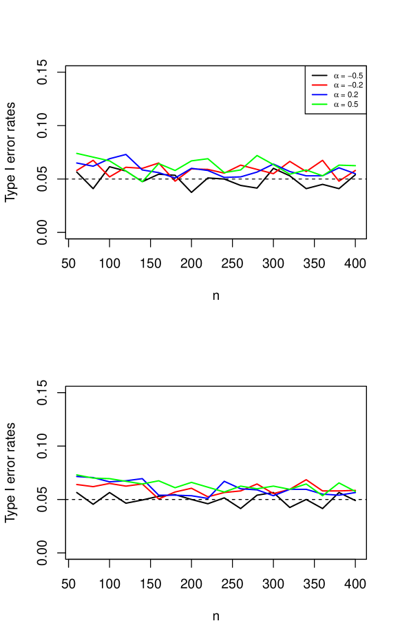
Figure 1: Empirical type I error rates (without model selection) of the test of level change (top) and the test of trend change (bottom) for data generated from zero-one inflated Beta time series with Gaussian copula and fitted by Gaussian copula models.

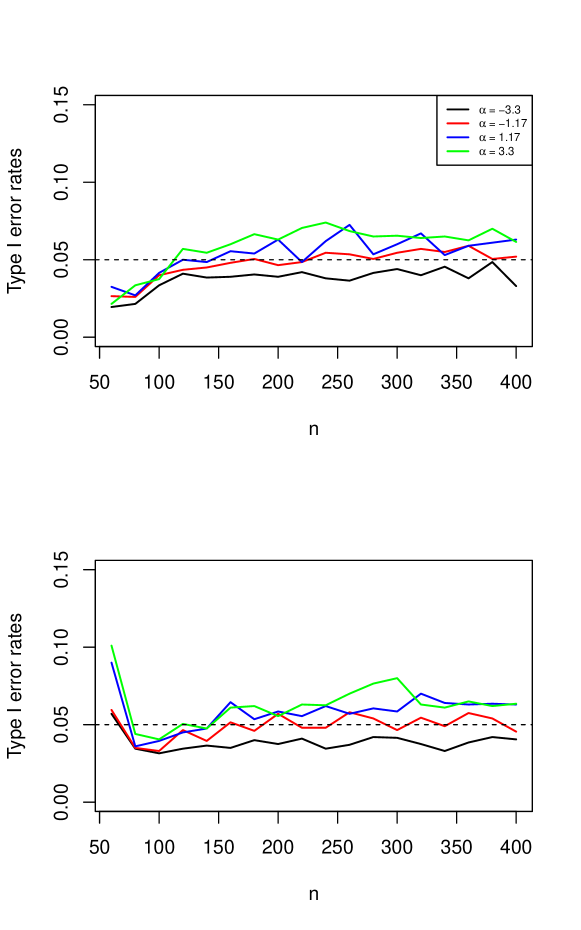
Figure 2: Empirical type I error rates (without model selection) of the test of level change (top) and the test of trend change (bottom) for data generated from zero-one inflated Beta time series with Frank copula and fitted by Gaussian copula models.

Figure 1 illustrates the simulation results for data generated from Gaussian copula models and fitted by Gaussian copula models (correct models). For all sample sizes and copula parameter values, the empirical type I error rates for both tests (level change and trend change) are close to the nominal level 0.05. Figure 2 illustrates the simulation results for data generated from Frank copula models but fitted by Gaussian copula models (misspecified models). The empirical type I error rates, except where $\rho=-1.17$ (corresponding to $\rho=-0.2$ for Gaussian copula), are in general less close to the nominal level than when models are correctly specified (Figure 1). Due to the model misspecification, when sample sizes are small, the empirical type I error rates are conservative for the test of level change but inflated for the test of trend change.

4.1.2 Simulation results

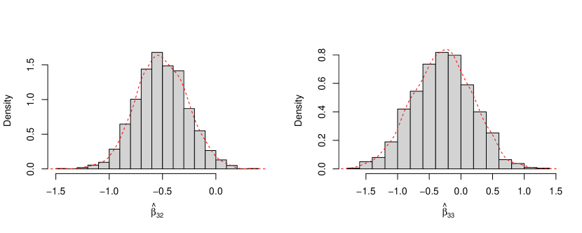
Figure 3: Empirical distributions of $\hat{\beta}_{32}$ (left) and $\hat{\beta}_{33}$ (right).

Figure 3 illustrates the empirical distributions of $\hat{\beta}_{32}$ and $\hat{\beta}_{33}$ when $n=60$. Both distributions are approximately normal, indicating that the proposed estimator is still valid for small sample sizes. Notice that the model misspecification on the copula model does not have an impact on the performance of point estimates on the marginal parameters because the independent likelihood estimator only depends on the marginal distribution of $\bm{Y}$.

We consider sample sizes of $n$ = 60, 120, or 180, and summarize the simulation results for data generated from Gaussian copula models and fitted by Gaussian copula models (correct models) in Table 2. For both estimators ($\hat{\beta}_{32}$ and $\hat{\beta}_{33}$), biases are close to 0 and negligible in all settings. Both standard error of estimates ($\mbox{SE}(\hat{\beta})$) and means of standard error estimates ($\mbox{E}(\widehat{\mbox{SE}})$) decrease, and power increases, as sample size increases or copula parameter, $\rho,$ decreases. The variance estimator tends to underestimate its empirical counterpart (i.e., $\mbox{E}(\widehat{\mbox{SE}})<\mbox{SE}(\hat{\beta})$) when $\rho=-0.2,0.2,0.5$. As a result, the actual coverage probabilities of 95% confidence intervals are lower than the nominal level in those settings. When $\rho=-0.5$, $\mbox{E}(\widehat{\mbox{SE}})$ are close to $\mbox{SE}(\hat{\beta})$ and coverage probabilities are close to nominal level. Due to the relatively small magnitude of $\beta_{33}$ (compare with $\beta_{32}$), the power of $\beta_{33}$ is much smaller than the power of $\beta_{32}$ in all settings.

Results for the misspecified models (data generated from Frank copula models but fitted by Gaussian copula models) are summarized in Table 3. Overall, our purposed estimator is robust against model misspecification. Similar to the correctly specified models, both estimators are almost unbiased. Moreover, $\mbox{SE}(\hat{\beta})$ and $\mbox{E}(\widehat{\mbox{SE}})$ decrease, and power increases, as sample size increases or $\rho$ decreases. When the sample size is small ($n=60$), the variance estimator of $\beta_{33}$ overestimates its empirical counterpart (i.e., $\mbox{E}(\widehat{\mbox{SE}})>\mbox{SE}(\hat{\beta})$), leading to low power in these scenarios.

4.2 Simulation results with model selection

We then consider the setting in which the change point is unknown but still equals to the time of policy intervention, and the model selection method described in Section 3.4 is used to for change point selection. For the propose of illustration, we only consider five candidate values of change point in the model selection: $\tau-2$, $\tau-1$, $\tau$, $\tau+1$, and $\tau+2$. In practice, we may want to include as many candidate values as possible to ensure the true value is included in the candidate set.

4.2.1 Type I error rate

We first investigate the type I error rate after model selection. Similar to Section 4.1.1, We also consider the sample sizes of $n=60,80,\cdots,400$.

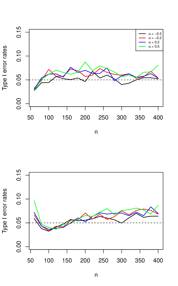
Figure 4: Empirical type I error rates (with model selection) of the test of level change (top) and the test of trend change (bottom) for data generated from zero-one inflated Beta time series with Gaussian copula and fitted by Gaussian copula models.

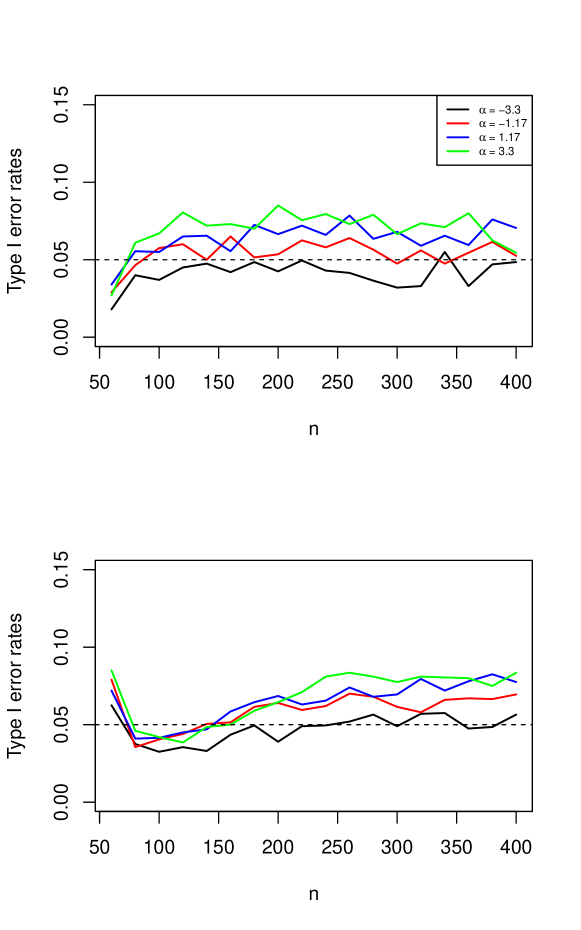
Figure 5: Empirical type I error rates (with model selection) of the test of level change (top) and the test of trend change (bottom) for data generated from zero-one inflated Beta time series with Frank copula and fitted by Gaussian copula models.

Figure 4 illustrates the simulation results for data generated from Gaussian copula models and fitted by Gaussian copula models (correct models), and Figure 5 illustrates the simulation results for data generated from Frank copula models but fitted by Gaussian copula models (misspecified models). At small sample sizes, the empirical type error rates are conservative for the test of level change but inflated for the test of trend change when sample sizes are small. In general, the empirical type I error rates after model selection are more inflated than their without model selection counterpart, because the method tends to select a model that maximizes the estimated effects of level and trend changes.

4.2.2 Simulation results

Table 4 presents the simulation results for data generated from Gaussian copula and fitted by Gaussian copula models (correct models) with sample sizes $n$ = 60, 120, or 180 are considered. Contrary to the results without model selection (Table 2), the proposed estimator is biased, and the bias decreases as sample size increases. As a result, the coverage probabilities of 95% CIs are lower than the corresponding coverage probabilities without model selection. Similar trends are observed for other measures: $\mbox{SE}(\hat{\beta})$ and $\mbox{E}(\widehat{\mbox{SE}})$ decrease as sample size increases or copula parameter $\rho$ decreases, and coverage probabilities and power increase as sample size increases.

Simulation results for data generated from Frank copula and fitted by Gaussian copula models (misspecified models) are summarized in Table 5. Biases of both estimators are similar to the results of the correct models with model selection (Table 4), which again verifies the robustness of the Gaussian copula model. $\mbox{SE}(\hat{\beta})$ and $\mbox{E}(\widehat{\mbox{SE}})$ decrease, and power increases, as sample size increases or copula parameter $\rho$ decreases. Although we observe very small powers for $\beta_{33}$ when $n=60$ in Table 3 (misspecified models without model selection), such result is not observed with model selection.

5 ITS analysis of the intervention effect on patient ‘pain management’ scores

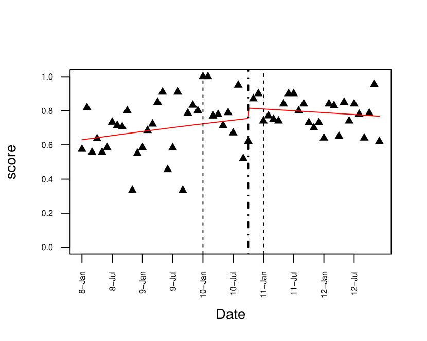
Figure 6: The time series of observed ‘pain management’ scores for a single hospital, the estimated change point, estimated means, and boundaries of possible change points. The estimated means and change point are obtained from modeling the time series with MZOIBTS.

Patient ‘pain management’ scores of a single hospital are modeled using our proposed MZOIBTS model. Figure 6 illustrates the data used for this analysis.

We consider the models suggested in Section 2.3, where the marginal mean of the time series (which is the main model in ITS analysis) is assumed as in model (16) with $T(t)=t$. We present results based on the Gaussian copula, but other copula functions result in similar conclusions. We assume the change point of the intervention effect can happen anytime between January 2010 and January 2011, i.e., 6 months before and after the formal intervention time.

Figure 6 shows the fitted mean function, and the resulting parameter estimates are given in Table 6. The estimated change point occurs in October 2010, about 4 months after the formal implementation time, indicating that the implementation of the intervention requires a period of time to reach its full extent. The estimated ‘pain management’ score is initiated at 62.9% and gradually increases to 75.4% before the estimated change point (October 2010). A 6% increase in the estimated ‘pain management’ score is observed immediately after the estimated change point, but the score then gradually decreases to 76.8% by the end of the follow-up period. However, the two key parameters measuring level change ($\beta_{32}$) and trend change ($\beta_{33}$) are not statistically significant at the $\alpha=0.05$ level ($p$-values: 0.265 and 0.103 respectively).

Our results reveal a significant increase on the dispersion parameter $\phi_{t}$ ($\beta_{41}=0.795$, $p$-value = 0.024). According to the second equation in (2.1), an increase in $\phi_{t}$ results in a reduction in the standard deviation of the outcome. In this study, the average estimated standard deviation of $Y_{t}$ decreases from 0.143 before intervention to 0.110 after the change point.

6 Discussion

In this article, motivated by ITS analysis, we propose a copula-based time series model for zero-one-inflated proportional data analysis, and develop a two-stage estimation procedure for parameter estimation and statistical inference. Our simulation results reveal that our proposed method is still valid at a small sample size ($n=60$). We apply the proposed MZOIBTS model to study the impact of a new nursing care delivery mode on the patients’ ‘pain management’ scores of a single hospital unit. Although we do not find any significant changes on the level and trend of ‘pain management’ scores after intervention, the variance of the scores significantly decreases after the change point. As pointed out by Cruz et al., (2017), the reduction on the variance can be considered as a positive result of the intervention since it leads to more stable scores.

We focus on the estimation and inference of the marginal model parameters, while the copula parameter is considered as nuisance and is being estimated separately. Although we can select the optimal copula function by maximizing the second step objective function, it can be computationally expensive due to the slow convergence for some of the copula functions. We suggest considering the Gaussian copula as the default choice. The robustness of the use of the Gaussian copula function against model misspecification has been verified by our simulation results. Moreover, different copula functions also result in similar inferences and conclusions in our real data analysis.

Our analysis does not detect any level or trend changes after intervention. This can be due to the ceiling effect, where the mean score will stop increasing after it reaches its maximum. On the one hand, our proposed model partially addresses the ceiling effect by bounding the marginal means of outcomes to 0 and 1. On the other hand, however, we assume an unstationary time series with the deterministic specified as the generalized segmented linear regression model (16). It assumes the logit-transformed marginal mean $v_{t}$ keeps increasing/decreasing as $t$ increases if $\beta_{31}+\beta_{33}\neq 0$, but in practice, it is possible that the time series will become stationary after $v_{t}$ reaches a certain level. Thus, it is of great interest to investigate new models to include this ceiling/flooring effect.

Finally, some other models can also be considered for such bounded outcomes. For example, the tilted Beta distribution proposed by Hahn, (2021) is an alternative distribution for bounded outcomes with multiple zeros or ones. We can also assume the outcomes are censored at zero and one, and marginalized Tobit regression models Wang and Griswold, (2017) can be used to analyze such data. It is of interest to incorporate serial dependence in these models.

Table 1: Bivariate copula functions.

Copula	Copula function
Gaussian	$C(u_{1},u_{2};\rho)=\Phi_{\rho}(\Phi^{-1}(u_{1}),\Phi^{-1}(u_{2}))$, $\rho\in[-1,1]$
Clayton	$C(u_{1},u_{2};\rho)=\max(0,(u_{1}^{-\rho}+u_{2}^{-\rho}-1)^{-1/\rho})$, $\rho\geq-1$
Gumbel	$C(u_{1},u_{2};\rho)=\exp\{-[(-\log u_{1})^{\rho}+(-\log u_{1})^{\rho}]^{1/\rho}\}$, $\rho\geq 1$
Frank	$C(u_{1},u_{2};\rho)=-\frac{1}{\rho}\log\left\{1+\frac{[\exp(-\rho u_{1})-1][\exp(-\rho u_{2})-1]}{\exp(-\rho-1)}\right\}$, $\rho\in\mathbb{R}/\{0\}$
Ali-Mikhail-Haq (AMH)	$C(u_{1},u_{2};\rho)=\frac{u_{1}u_{2}}{1-\rho(1-u_{1})(1-u_{2})}$, $\rho\in[-1,1]$

Table 2: Bias, standard error of $\hat{\beta}$ ($\mbox{SE}(\hat{\beta})$), mean of standard error estimates ($\mbox{E}(\widehat{\mbox{SE}})$), 95% confidence interval coverage probability (Cov.prob), and power for data generated from zero-one inflated Beta time series with Gaussian copula and fitted by Gaussian copula models.

$n$	Bias		$\mbox{SE}(\hat{\beta})$		$\mbox{E}(\widehat{\mbox{SE}})$		Cov.prob		Power
	$\beta_{32}$	$\beta_{33}$	$\beta_{32}$	$\beta_{33}$	$\beta_{32}$	$\beta_{33}$	$\beta_{32}$	$\beta_{33}$	$\beta_{32}$	$\beta_{33}$
	$\rho=0.2$
60	-0.002	-0.008	0.224	0.431	0.208	0.401	0.924	0.921	0.656	0.149
120	-0.001	-0.007	0.155	0.299	0.150	0.289	0.936	0.935	0.900	0.192
180	-0.001	0.000	0.128	0.249	0.124	0.238	0.934	0.937	0.972	0.272
	$\rho=0.5$
60	-0.009	0.011	0.237	0.471	0.222	0.431	0.931	0.924	0.617	0.138
120	-0.004	0.004	0.170	0.327	0.164	0.316	0.938	0.934	0.855	0.177
180	0.001	0.003	0.136	0.275	0.134	0.258	0.935	0.931	0.952	0.232
	$\rho=-0.2$
60	-0.010	0.001	0.194	0.364	0.181	0.347	0.924	0.938	0.775	0.155
120	-0.001	-0.007	0.135	0.254	0.128	0.245	0.938	0.939	0.967	0.248
180	-0.002	-0.001	0.107	0.204	0.105	0.199	0.937	0.933	0.997	0.330
	$\rho=-0.5$
60	-0.002	-0.001	0.165	0.314	0.167	0.316	0.949	0.945	0.848	0.160
120	0.000	-0.005	0.114	0.214	0.116	0.219	0.947	0.958	0.991	0.288
180	0.000	0.001	0.092	0.173	0.093	0.176	0.950	0.948	0.999	0.387

Table 3: Bias, standard error of $\hat{\beta}$ ($\mbox{SE}(\hat{\beta})$), mean of standard error estimates ($\mbox{E}(\widehat{\mbox{SE}})$), 95% confidence interval coverage probability (Cov.prob), and power for data generated from zero-one inflated Beta time series with Frank copula and fitted by Gaussian copula models.

$n$	Bias		$\mbox{SE}(\hat{\beta})$		$\mbox{E}(\widehat{\mbox{SE}})$		Cov.prob		Power
	$\beta_{32}$	$\beta_{33}$	$\beta_{32}$	$\beta_{33}$	$\beta_{32}$	$\beta_{33}$	$\beta_{32}$	$\beta_{33}$	$\beta_{32}$	$\beta_{33}$
	$\rho=1.17$
60	0.013	0.001	0.193	0.352	0.246	0.937	0.968	0.928	0.625	0.021
120	-0.003	-0.004	0.136	0.247	0.140	0.404	0.943	0.918	0.954	0.160
180	0.000	-0.001	0.110	0.198	0.108	0.230	0.928	0.922	0.992	0.324
	$\rho=3.3$
60	0.008	0.011	0.209	0.382	0.282	1.069	0.973	0.931	0.523	0.009
120	-0.007	0.009	0.148	0.265	0.155	0.480	0.949	0.918	0.925	0.133
180	-0.001	-0.002	0.123	0.218	0.118	0.265	0.921	0.922	0.984	0.275
	$\rho=-1.17$
60	0.006	-0.001	0.163	0.280	0.215	0.820	0.961	0.956	0.754	0.034
120	-0.004	0.002	0.112	0.198	0.118	0.343	0.944	0.932	0.991	0.212
180	-0.000	-0.003	0.089	0.160	0.092	0.191	0.933	0.933	1.000	0.436
	$\rho=-3.3$
60	0.008	0.004	0.140	0.253	0.198	0.765	0.971	0.952	0.807	0.036
120	-0.002	-0.005	0.093	0.168	0.106	0.321	0.963	0.951	0.998	0.270
180	0.001	-0.002	0.077	0.131	0.083	0.172	0.954	0.949	1.000	0.519

Table 4: Bias, standard error of $\hat{\beta}$ ($\mbox{SE}(\hat{\beta})$), mean of standard error estimates ($\mbox{E}(\widehat{\mbox{SE}})$), 95% confidence interval coverage probability (Cov.prob), and power for data generated from zero-one inflated Beta time series with Gaussian copula and fitted by Gaussian copula models.

$n$	Bias		$\mbox{SE}(\hat{\beta})$		$\mbox{E}(\widehat{\mbox{SE}})$		Cov.prob		Power
	$\beta_{32}$	$\beta_{33}$	$\beta_{32}$	$\beta_{33}$	$\beta_{32}$	$\beta_{33}$	$\beta_{32}$	$\beta_{33}$	$\beta_{32}$	$\beta_{33}$
	$\rho=0.2$
60	0.212	-0.036	0.243	1.062	0.288	0.981	0.898	0.850	0.239	0.137
120	0.109	-0.153	0.157	0.336	0.144	0.414	0.847	0.839	0.750	0.336
180	0.049	-0.079	0.123	0.216	0.110	0.232	0.873	0.869	0.966	0.451
	$\rho=0.5$
60	0.203	0.089	0.261	1.201	0.329	1.058	0.926	0.840	0.214	0.136
120	0.102	-0.140	0.173	0.384	0.159	0.488	0.846	0.849	0.684	0.243
180	0.050	-0.075	0.136	0.253	0.120	0.275	0.876	0.860	0.940	0.381
	$\rho=-0.2$
60	0.227	-0.107	0.221	0.935	0.246	0.835	0.852	0.849	0.268	0.181
120	0.110	-0.158	0.136	0.276	0.122	0.348	0.807	0.813	0.840	0.427
180	0.048	-0.076	0.105	0.192	0.093	0.191	0.856	0.845	0.994	0.554
	$\rho=-0.5$
60	0.231	-0.146	0.194	0.862	0.239	0.801	0.833	0.841	0.279	0.201
120	0.105	-0.163	0.118	0.231	0.110	0.332	0.798	0.804	0.915	0.495
180	0.046	-0.070	0.094	0.163	0.083	0.177	0.854	0.862	0.999	0.631

Table 5: Bias, standard error of $\hat{\beta}$ ($\mbox{SE}(\hat{\beta})$), mean of standard error estimates ($\mbox{E}(\widehat{\mbox{SE}})$), 95% confidence interval coverage probability (Cov.prob), and power for data generated from zero-one inflated Beta time series with Frank copula and fitted by Gaussian copula models.

$n$	Bias		$\mbox{SE}(\hat{\beta})$		$\mbox{E}(\widehat{\mbox{SE}})$		Cov.prob		Power
	$\beta_{32}$	$\beta_{33}$	$\beta_{32}$	$\beta_{33}$	$\beta_{32}$	$\beta_{33}$	$\beta_{32}$	$\beta_{33}$	$\beta_{32}$	$\beta_{33}$
	$\rho=1.17$
60	0.222	-0.054	0.240	1.003	0.291	0.975	0.900	0.854	0.230	0.131
120	0.111	-0.169	0.161	0.329	0.145	0.425	0.830	0.817	0.740	0.329
180	0.042	-0.066	0.126	0.250	0.110	0.232	0.883	0.865	0.967	0.435
	$\rho=3.3$
60	0.217	0.025	0.270	1.166	0.330	1.063	0.920	0.855	0.209	0.127
120	0.103	-0.153	0.178	0.375	0.159	0.483	0.852	0.864	0.698	0.264
180	0.045	-0.072	0.135	0.241	0.120	0.260	0.878	0.875	0.945	0.387
	$\rho=-1.17$
60	0.225	-0.092	0.194	0.941	0.246	0.855	0.852	0.855	0.270	0.175
120	0.103	-0.158	0.133	0.245	0.122	0.356	0.812	0.835	0.870	0.440
180	0.048	-0.070	0.103	0.184	0.093	0.194	0.873	0.869	0.996	0.545
	$\rho=-3.3$
60	0.229	-0.147	0.178	0.855	0.234	0.801	0.827	0.851	0.271	0.201
120	0.108	-0.167	0.116	0.245	0.110	0.324	0.790	0.805	0.925	0.507
180	0.050	-0.072	0.089	0.181	0.084	0.173	0.879	0.853	0.999	0.647

Table 6: The 95% confidence intervals, $p$-values, and estimates of the mean parameters.

Parameters	Point estimates	95% Confidence Intervals	$p$-values
$\beta_{30}$: initial level	$0.512$	$(0.075,0.948)$	0.021
$\beta_{31}$: initial trend	$0.018$	$(-0.005,0.041)$	0.119
$\beta_{32}$: level change	$0.362$	$(-0.275,1.000)$	0.265
$\beta_{33}$: trend change	$-0.029$	$(-0.064,0.006)$	0.103
$\beta_{40}$: initial dispersion	$2.196$	$(1.715,2.677)$	0.000
$\beta_{41}$: dispersion change	$0.795$	$(0.104,1.486)$	0.024

References

- Abdel-Karim, (2017) Abdel-Karim, A. H. (2017). Extended zero-one inflated beta and adjusted three-part regression models for proportional data analysis. Communications in Statistics-Simulation and Computation, 46(8):6155–6172.
- Alqawba and Diawara, (2021) Alqawba, M. and Diawara, N. (2021). Copula-based markov zero-inflated count time series models with application. Journal of Applied Statistics, 48(5):786–803.
- Bender et al., (2012) Bender, M., Connelly, C. D., Glaser, D., and Brown, C. (2012). Clinical nurse leader impact on microsystem care quality. Nursing Research, 61(5):326–332.
- Bender et al., (2015) Bender, M., Murphy, E., Thomas, T., Kaminski, J., and Smith, B. (2015). Clinical nurse leader integration into care delivery microsystems: quality and safety outcomes at the unit and organization level. In Academy Health Annual Research Meeting.
- Bender et al., (2019) Bender, M., Murphy, E. A., Cruz, M., and Ombao, H. (2019). System-and unit-level care quality outcome improvements after integrating clinical nurse leaders into frontline care delivery. JONA: the Journal of Nursing Administration, 49(6):315–322.
- Bender et al., (2017) Bender, M., Williams, M., Su, W., and Hites, L. (2017). Refining and validating a conceptual model of clinical nurse leader integrated care delivery. Journal of Advanced Nursing, 73(2):448–464.
- Bernal et al., (2017) Bernal, J. L., Cummins, S., and Gasparrini, A. (2017). Interrupted time series regression for the evaluation of public health interventions: a tutorial. International journal of epidemiology, 46(1):348–355.
- Casarin et al., (2012) Casarin, R., Dalla Valle, L., and Leisen, F. (2012). Bayesian model selection for beta autoregressive processes. Bayesian Analysis, 7(2):385–410.
- Chai et al., (2018) Chai, H., Jiang, H., Lin, L., and Liu, L. (2018). A marginalized two-part beta regression model for microbiome compositional data. PLoS computational biology, 14(7):e1006329.
- Chandler and Bate, (2007) Chandler, R. E. and Bate, S. (2007). Inference for clustered data using the independence loglikelihood. Biometrika, 94(1):167–183.
- Cook et al., (2002) Cook, T. D., Campbell, D. T., and Shadish, W. (2002). Experimental and quasi-experimental designs for generalized causal inference. Houghton Mifflin Boston, MA.
- Cruz et al., (2017) Cruz, M., Bender, M., and Ombao, H. (2017). A robust interrupted time series model for analyzing complex health care intervention data. Statistics in medicine, 36(29):4660–4676.
- Cruz et al., (2019) Cruz, M., Gillen, D. L., Bender, M., and Ombao, H. (2019). Assessing health care interventions via an interrupted time series model: study power and design considerations. Statistics in medicine, 38(10):1734–1752.
- Da-Silva and Migon, (2016) Da-Silva, C. Q. and Migon, H. S. (2016). Hierarchical dynamic beta model. Revstat Statistical Journal, 14(1):49–73.
- Davis et al., (2003) Davis, R. A., Dunsmuir, W. T., and Streett, S. B. (2003). Observation-driven models for poisson counts. Biometrika, 90(4):777–790.
- Davison and Hinkley, (1997) Davison, A. C. and Hinkley, D. V. (1997). Bootstrap methods and their application. Number 1. Cambridge university press.
- Fang and Ma, (2013) Fang, K. and Ma, S. (2013). Three-part model for fractional response variables with application to chinese household health insurance coverage. Journal of Applied Statistics, 40(5):925–940.
- Ferrari and Cribari-Neto, (2004) Ferrari, S. and Cribari-Neto, F. (2004). Beta regression for modelling rates and proportions. Journal of applied statistics, 31(7):799–815.
- Fokianos et al., (2009) Fokianos, K., Rahbek, A., and Tjøstheim, D. (2009). Poisson autoregression. Journal of the American Statistical Association, 104(488):1430–1439.
- Gao and Song, (2010) Gao, X. and Song, P. X.-K. (2010). Composite likelihood bayesian information criteria for model selection in high-dimensional data. Journal of the American Statistical Association, 105(492):1531–1540.
- Godambe, (1960) Godambe, V. P. (1960). An optimum property of regular maximum likelihood estimation. The Annals of Mathematical Statistics, 31(4):1208–1211.
- Gong and Samaniego, (1981) Gong, G. and Samaniego, F. J. (1981). Pseudo maximum likelihood estimation: theory and applications. The Annals of Statistics, pages 861–869.
- Guolo and Varin, (2014) Guolo, A. and Varin, C. (2014). Beta regression for time series analysis of bounded data, with application to canada google® flu trends. The Annals of Applied Statistics, 8(1):74–88.
- Hahn, (2021) Hahn, E. D. (2021). Regression modelling with the tilted beta distribution: A bayesian approach. Canadian Journal of Statistics, 49(2):262–282.
- Joe, (1997) Joe, H. (1997). Multivariate models and multivariate dependence concepts. CRC press.
- Joe, (2014) Joe, H. (2014). Dependence modeling with copulas. CRC press.
- Joe and Xu, (1996) Joe, H. and Xu, J. J. (1996). The estimation method of inference functions for margins for multivariate models. Technical Report 166, Department of Statistics, University of British Columbia.
- Kavanagh et al., (2012) Kavanagh, K. T., Cimiotti, J. P., Abusalem, S., and Coty, M.-B. (2012). Moving healthcare quality forward with nursing-sensitive value-based purchasing. Journal of Nursing Scholarship, 44(4):385–395.
- Kieschnick and McCullough, (2003) Kieschnick, R. and McCullough, B. D. (2003). Regression analysis of variates observed on (0, 1): percentages, proportions and fractions. Statistical modelling, 3(3):193–213.
- Kontopantelis et al., (2015) Kontopantelis, E., Doran, T., Springate, D. A., Buchan, I., and Reeves, D. (2015). Regression based quasi-experimental approach when randomisation is not an option: interrupted time series analysis. BMJ, 350:h2750.
- Masarotto and Varin, (2012) Masarotto, G. and Varin, C. (2012). Gaussian copula marginal regression. Electronic Journal of Statistics, 6:1517–1549.
- Nelsen, (2007) Nelsen, R. B. (2007). An introduction to copulas. Springer Science & Business Media.
- Ospina and Ferrari, (2012) Ospina, R. and Ferrari, S. L. (2012). A general class of zero-or-one inflated beta regression models. Computational Statistics & Data Analysis, 56(6):1609–1623.
- Penfold and Zhang, (2013) Penfold, R. B. and Zhang, F. (2013). Use of interrupted time series analysis in evaluating health care quality improvements. Academic pediatrics, 13(6):S38–S44.
- Rhee et al., (2021) Rhee, C., Wang, R., Ye, S., Baker, M. A., Griesbach, D., Laskowski, K., and Klompas, M. (2021). Decline in sars-cov-2 infections among health care workers at 2 hospitals following rollout and administration of mrna vaccines. Open Forum Infectious Diseases, 8(8):ofab204.
- Sørensen, (2019) Sørensen, H. (2019). Independence, successive and conditional likelihood for time series of counts. Journal of Statistical Planning and Inference, 200:20–31.
- van Doormaal et al., (2009) van Doormaal, J. E., van den Bemt, P. M., Zaal, R. J., Egberts, A. C., Lenderink, B. W., Kosterink, J. G., Haaijer-Ruskamp, F. M., and Mol, P. G. (2009). The influence that electronic prescribing has on medication errors and preventable adverse drug events: an interrupted time-series study. Journal of the American Medical Informatics Association, 16(6):816–825.
- Varin et al., (2011) Varin, C., Reid, N., and Firth, D. (2011). An overview of composite likelihood methods. Statistica Sinica, pages 5–42.
- Varin and Vidoni, (2005) Varin, C. and Vidoni, P. (2005). A note on composite likelihood inference and model selection. Biometrika, 92(3):519–528.
- Wagner et al., (2002) Wagner, A. K., Soumerai, S. B., Zhang, F., and Ross-Degnan, D. (2002). Segmented regression analysis of interrupted time series studies in medication use research. Journal of clinical pharmacy and therapeutics, 27(4):299–309.
- Wang and Griswold, (2017) Wang, W. and Griswold, M. E. (2017). Natural interpretations in tobit regression models using marginal estimation methods. Statistical methods in medical research, 26(6):2622–2632.
- Ye et al., (2022) Ye, S., Wang, R., and Zhang, B. (2022). Comparison of estimation methods and sample size calculation for parameter-driven interrupted time series models with count outcomes. Health Services and Outcomes Research Methodology, pages 1–48.